Revision date: 4/11/93

Solitons and Geometry

S. P. Novikov

1

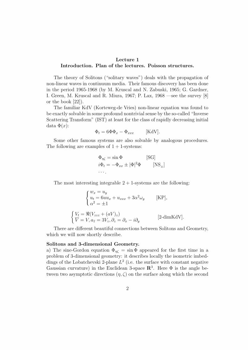
Lecture 1Introduction. Plan of the lectures. Poisson structures.

The theory of Solitons (“solitary waves”) deals with the propagation ofnon-linear waves in continuum media. Their famous discovery has been donein the period 1965-1968 (by M. Kruscal and N. Zabuski, 1965; G. Gardner,I. Green, M. Kruscal and R. Miura, 1967; P. Lax, 1968 —see the survey [8]or the book [22]).

The familiar KdV (Korteweg-de Vries) non-linear equation was found tobe exactly solvable in some profound nontrivial sense by the so-called “InverseScattering Transform” (IST) at least for the class of rapidly decreasing initialdata Φ(x):

Φt = 6ΦΦx − Φxxx [KdV].

Some other famous systems are also solvable by analogous procedures.The following are examples of 1 + 1-systems:

Φηζ = sin Φ [SG]

iΦt = −Φxx ± |Φ|2Φ [NS±]

· · · .

The most interesting integrable 2 + 1-systems are the following:

wx = uy

ut = 6uux + uxxx + 3α2ωy [KP],α2 = ±1

Vt = <(Vzzz + (aV )z)V = V, az = 3Vz, ∂z = ∂x − i∂y

[2-dimKdV].

There are different beautiful connections between Solitons and Geometry,which we will now shortly describe.

Solitons and 3-dimensional Geometry.a) The sine-Gordon equation Φηζ = sin Φ appeared for the first time in aproblem of 3-dimensional geometry: it describes locally the isometric imbed-dings of the Lobatchevski 2-plane L2 (i.e. the surface with constant negativeGaussian curvature) in the Euclidean 3-space R3. Here Φ is the angle be-tween two asymptotic directions (η, ζ) on the surface along which the second

2

(curvature) form is zero. It has been used by Bianchi, Lie and Backlund forthe construction of new imbeddings (“Backlund transformations”, discoveredby Bianchi).b) The elliptic equation

4Φ = sinh Φ

appeared recently for the description of genus 1 surfaces (“topological tori”)in R3 with constant mean curvature (H. Wente, 1986; R. Walter, 1987).

Starting from 1989 F. Hitchin, U. Pinkall, N. Ercolani, H. Knorrer, E.Trubowitz, A. Bobenko used in this field the technique of the “periodic IST”—see [5].

Solitons and algebraic geometry.a) There is a famous connection of Soliton theory with algebraic geometry.It appeared in 1974-1975 . The solution of the periodic problems of Solitontheory led to beautiful analytical constructions involving Riemann surfacesand their Jacobian varieties, Θ-functions and later also Prym varieties andso on (S. Novikov, 1974; B. Dubrovin - S.Novikov, 1974; B. Dubrovin, 1975;A. Its - V. Matveev,1975; P. Lax, 1975; H. McKean - P. Van Moerbeke, 1975—see [8]).

Many people worked in this area later (see [22], [8], [7] and [6]). Veryimportant results were obtained in different areas, including classical prob-lems in the theory of Θ-functions and construction of the harmonic analysison Riemann surfaces in connection with the “string theory” —see [15], [16],[17] and [6].b) Some very new and deep connection of the KdV theory with the topologyof the moduli spaces of Riemann surfaces appeared recently in the worksof M. Kontzevich (1992) in the development of the so-called “2-d quantumgravity”. It is a byproduct of the theory of “matrix models” of D. Gross-A.Migdal, E. Bresin-V. Kasakov and M. Duglas - N. Shenker, in which Solitontheory appeared as a theory of the “renormgroup” in 1989-90.

Soliton theory and Riemannian geometry.Let us recall that the systems of Soliton theory (like KdV) sometimes describethe propagation of non-linear waves. For the solution of some problems weare going to develop an asymptotic method which may be considered as anatural non-linear analogue of the famous WKB approximation in QuantumMechanics. It leads to the structures of Riemannian Geometry; some nice

3

classes of infinite-dimensional Lie algebras appeared in this theory. This willbe exactly the subject of the present lectures (see also [10]). All beautifulconstructions of Soliton theory are available for Hamiltonian systems only(nobody knows why). Therefore we will start with an elementary introductionto Symplectic and Poisson Geometry (see also [21], [7], [10] and [11]).

Plan of the lectures.

1. Symplectic and Poisson structures on finite-dimensional manifolds. Diracmonopole in classical mechanics. Complete integrability and Algebraic Ge-ometry.2. Local Poisson Structures on loop spaces. First-order structures and finitedimensional Riemannian Geometry. Hydrodynamic-Type systems. Infinite-dimensional Lie Algebras. Riemann Invariants and classical problems of dif-ferential Geometry. Orthogonal coordinates in Rn.3. Nonlinear analogue of the WKB-method. Hydrodynamics of SolitonLattices. Special analysis for the KdV equation. Dispersive analogue ofthe shock wave. Genus 1 solution for the hydrodynamics of Soliton Lattices.

4

Symplectic and Poisson structures

Let M be a finite-dimensional manifold with a system (y1, . . . , ym) of (local)coordinates.Definition. Any non-degenerate closed 2-form

Ω = ωαβdyα ∧ dyβ

generates a symplectic structure on the manifold M . Non-degeneracy meansexactly that the skew-symmetric matrix (ωαβ) is non-singular for all pointsy ∈ M , i.e.

det(ωαβ(y)) 6= 0.

Remark. Since a skew-symmetric matrix in odd dimension is necessarilysingular we have that if M has a symplectic structure then it has even di-mension.

By definition a symplectic structure is just a special skew-symmetricscalar product of the tangent vectors: if V = (V α) and W = (W β) arecoordinates of tangent vectors we set:

(V,W ) = ωαβV αW β = −(W,V ).

Let ωαβ denote the inverse matrix:

ωαβωβγ = δαβ .

This inverse matrix (ωαβ) determines everything important in the theory ofHamiltonian systems. Therefore we shall start with the following definition.Definition. A skew-symmetric C∞-tensor field (ωαβ) on the manifold Mgenerates a Poisson structure if the Poisson bracket (defined below) turnsthe space C∞(M) into a Lie algebra: for any two functions f, g ∈ C∞(M) wedefine their Poisson bracket as a scalar product of the gradients:

f, g = ωαβ ∂f

∂yα

∂g

∂yβ = −g, f.

This operation obviously satisfies the following requirements:

f, g = −g, f,f + g, h = f, h + g, h,fg, h = fg, h + gf, h,

5

so only the Jacobi identity is non-obvious.Remark. Using the coordinate functions we have that

yα, yβ = ωαβ

yα, yβ, yγ =∂ωαβ

∂yk

∂yγ

∂yp ωkp =∂ωαβ

∂yk ωkγ

and it is easily checked that the Jacobi identity is equivalent to:

∂ωαβ

∂yk ωkγ +∂ωγα

∂yk ωkβ +∂ωβγ

∂yk ωkα = 0 ∀α, β, γ.

In case (ωαβ) is non-singular and (ωαβ) denotes the inverse matrix this is alsoequivalent to:

∂ωαβ

∂yγ +∂ωγα

∂yβ +∂ωβγ

∂yα = 0 ∀α, β, γ

i.e. to

d

∑

α<β

ωαβdyα ∧ dyβ

= 0

i.e. to closedness of the 2-form ωαβdyα∧dyβ. (Recall however that the inversematrix does not exist in some important cases.)Definition. A function f ∈ C∞(M) is called a Casimir for the given Poissonbracket if it belongs to the kernel (or annihilator) of the Poisson bracket, i.e.if for any function g ∈ C∞(M) we have

f, g = 0.

6

Lecture 2.

Poisson Structures on Finite-dimensional Manifolds.Hamiltonian Systems. Completely Integrable Systems.

As in Lecture 1 we are dealing with a finite-dimensional manifold M with(local) coordinates (y1, . . . , ym) and a Poisson tensor field −ωij = ωji suchthat the corresponding Poisson bracket

f, g = ωij ∂t

∂yi

∂g

∂yj

generates a Lie algebra structure on the space C∞(M).Definition. Any smooth function H(y) on M or a closed 1-form Hαdyα

generates a Hamiltonian system by the formula

yα = ωαβHβ

(

Hβ =∂H

∂yβ

)

.

For any function f ∈ C∞(M) we define

f = f,H = ωαβHβfα.

Definition. We will say a vector field V with coordinates (V α) is a Hamil-tonian vector field generated by the Hamiltonian H ∈ C∞(M) if V α =wβα∂H/∂yβ.

A well-known lemma states that the commutator of any pair of Hamil-tonian vector fields is also Hamiltonian and it is generated by the Poissonbracket of the corresponding Hamiltonians.

We define a Poisson algebra as a commutative associative algebra C withan additional Lie algebra operation (“bracket”)

C × C 3 (f, g) 7→ f, g ∈ C

such thatf · g, h = f · g, h + g · f, h.

Definition. We call integral of a Hamiltonian system a function f such thatf = 0.

7

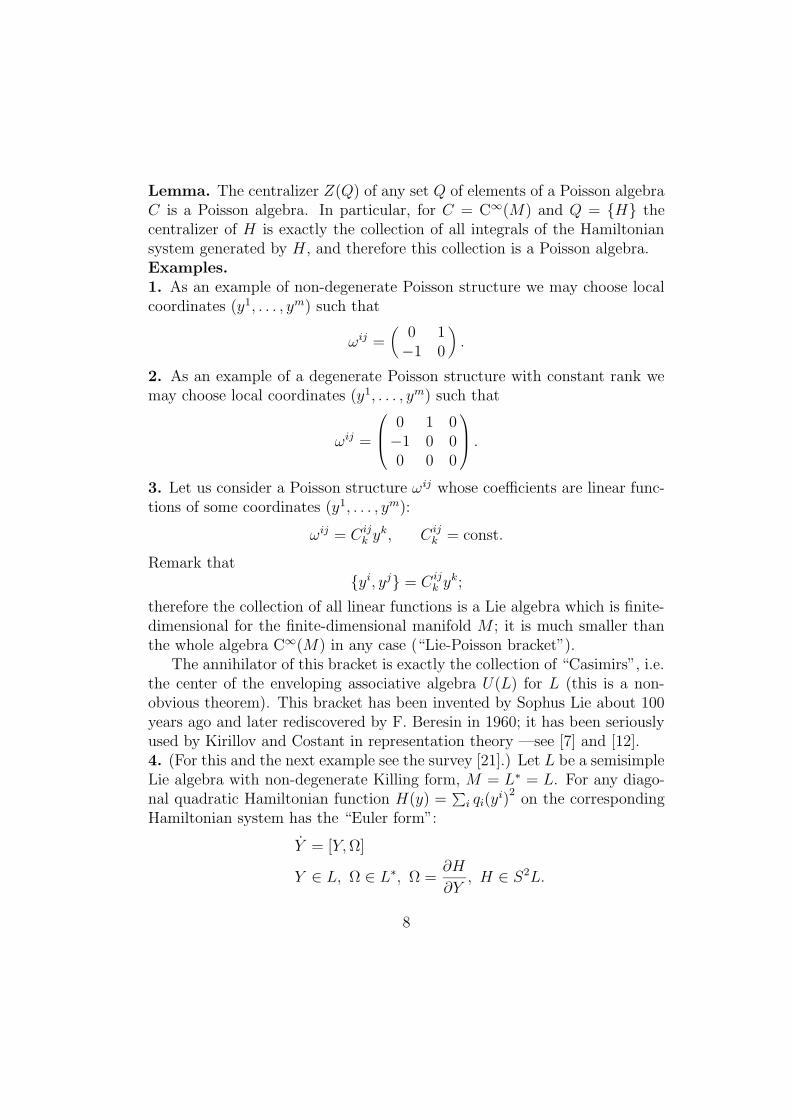
Lemma. The centralizer Z(Q) of any set Q of elements of a Poisson algebraC is a Poisson algebra. In particular, for C = C∞(M) and Q = H thecentralizer of H is exactly the collection of all integrals of the Hamiltoniansystem generated by H, and therefore this collection is a Poisson algebra.Examples.1. As an example of non-degenerate Poisson structure we may choose localcoordinates (y1, . . . , ym) such that

ωij =(

0 1−1 0

)

.

2. As an example of a degenerate Poisson structure with constant rank wemay choose local coordinates (y1, . . . , ym) such that

ωij =

0 1 0−1 0 00 0 0

.

3. Let us consider a Poisson structure ωij whose coefficients are linear func-tions of some coordinates (y1, . . . , ym):

ωij = C ijk yk, C ij

k = const.

Remark thatyi, yj = C ij

k yk;

therefore the collection of all linear functions is a Lie algebra which is finite-dimensional for the finite-dimensional manifold M ; it is much smaller thanthe whole algebra C∞(M) in any case (“Lie-Poisson bracket”).

The annihilator of this bracket is exactly the collection of “Casimirs”, i.e.the center of the enveloping associative algebra U(L) for L (this is a non-obvious theorem). This bracket has been invented by Sophus Lie about 100years ago and later rediscovered by F. Beresin in 1960; it has been seriouslyused by Kirillov and Costant in representation theory —see [7] and [12].4. (For this and the next example see the survey [21].) Let L be a semisimpleLie algebra with non-degenerate Killing form, M = L∗ = L. For any diago-nal quadratic Hamiltonian function H(y) =

∑

i qi(yi)

2on the corresponding

Hamiltonian system has the “Euler form”:

Y = [Y, Ω]

Y ∈ L, Ω ∈ L∗, Ω =∂H

∂Y, H ∈ S2L.

8

Suppose L = son. In this case the index (i) is exactly the pair

i = (α, β), α < β, α, β = 1, . . . , n, m = n(n − 1)/2.

By [1] the generalized “rigid body” system corresponds to the case:

qi = q(α,β) = qα + qβ, qα ≥ 0.

More generally, let two collections of numbers

a1, . . . , an, b1, . . . , bn

be given in such a way that

qi = q(α,β) =aα − aβ

bα − bβ

, α < β.

The Euler system in this case admits the following so-called “λ-representation”(analogous to the one constructed in 1974 for the finite-gap solutions of KdVand the finite-gap potentials of the Schrodinger operator):

∂t(Y − λU) = [Y − λU, Ω − λV ].

Here Y and Ω are skew-symmetric matrices and

U = diag(a1, . . . , an), V = diag(b1, . . . , bn)

(Manakov, 1976).The collection of conservation laws might be obtained from the coefficients

of the algebraic curve Γ:

Γ : det(Y − λU − µ1) = P (λ, µ) = 0.

We shall return to this type of examples later. Remark that a Riemannsurface already appeared here.5. Consider now the Lie algebra L of the group E3 (the isometry group ofeuclidean 3-space R3). The Lie algebra L is 6-dimensional: it has a set ofgenerators M 1,M 2,M 3, p1

, p2, p

3 satisfying the relations:

[M i,M j] = εijkMk, εijk = ±1,

[M i, pj] = εijkpk

,

[pi, p

j] = 0.

9

We set M = L = L∗ and we denote by Mi and pi the coordinates along M i

and pirespectively. There are exactly two independent functions

f1 = p2 =∑

i

p2i , f2 = ps =

∑

i

Mipi

such thatfα, C∞(M) = 0 α = 1, 2.

We shall consider later the Hamiltonians

a) 2H =∑

aiM2i +

∑

bij(piMj + Mipj) +∑

cijpipj;

b) 2H =∑

aiM2i + 2W (lipi);

(in case b we have p2 = 1).Definition. A Hamiltonian system is called completely integrable in thesense of Liouville if it admits a “large enough” family of independent inte-grals which are in involution (i.e. have trivial pairwise Poisson brackets),where “large enough” means exactly (dimM)/2 for non-degenerate Poissonstructures (symplectic manifolds ) or k + s if dimM = 2k + s and the rankof the Poisson tensor (ωij) is equal to 2k.

Let us fix for the sequel a completely integrable Hamiltonian system anda family f1, ..., fk+s of integrals as in the definition. The gradients of theseintegrals are linearly independent at the generic point. Therefore the genericlevel surface:

f1 = c1

· · ·fk+s = ck+s

(where the ci’s are constants) is a k-dimensional non-singular manifold N k

in M .Theorem. The manifold N k is the factor of Rk by a lattice:

Nk = Rk/Γ.

On Nk there are natural coordinates (ϕ1, . . . , ϕk) such that ϕi = const.Corollary. If the level surface N k is compact then it is diffeomorphic to thetorus T k = (S1)k.

Let us assume now that s = 0, i.e. that the tensor (ωij) is invertible. Asusual we denote by Ω the (closed) 2-form with local expression

∑

i<j ωijdyi ∧

10

dyj where by definition ωilωlj = δij. Let us consider a compact level surface

Nk. In a small neighborhood U(N k) in M we may introduce an important1-form ω such that

dω = Ω

(Ω = 0 on Nk). In the domain U(N k) there exist “action-angle” coordinates

(ϕ1, . . . , ϕk, s1, . . . , sk)

such thatϕi, ϕj = si, sj = 0, ϕi, sj = δij,

|si| ≤ 1/(2π)∮

γi

ω, 0 ≤ ϕi ≤ 2π.

Here γi ∈ H1(Nk,Z) is the basic cycle on the torus N k represented by the

coordinates:(ϕ1, ..., ϕk), 0 ≤ ϕi ≤ 2π, ϕj = 0 for j 6= i.

11

Lecture 3

Classical Analogue of the Dirac Monopole.Complete Integrability and Algebraic Geometry.

1. Let us consider again the important Example 5 of Lecture 2. Let L∗ = Mwhere L is the Lie algebra of the group E3; L has six generators (M 1,M 2,M3, p1

, p2, p

3)

and two “Casimirs”

ps =∑

Mipi = f2, p2 =∑

p2i = f1.

We recall that this means the following:

f1, C∞(M) = 0, f2, C

∞(M) = 0

The ordinary top in the constant gravity field might be considered as a systemon this phase space corresponding to the Hamiltonian:

2H =∑

i

aiM2i + gp3, p2 = 1.

The original phase space is T ∗(SO(3)). There is at least one additionalintegral of motion apart from energy (“area integral”) because the gravityforce is axially symmetric in this case. Consider now the Poisson subalgebraA of C∞(T ∗(SO(3)) which annihilates the area integral: A = Z(f).Lemma. The algebra A is isomorphic to C∞(M) factorized by the relation(p2 = 1). Here M = L∗ and L is the Lie algebra of the group E3. Thefunction f ∈ A corresponds to the Casimir element

f2 = ps =∑

Mipi

(the restriction p2 = 1 has to be added). For any value s = f2 this algebra isnaturally isomorphic to C∞(T ∗(S2)) as a commutative algebra.Proof. The conclusion is obvious in case

∑

i Mipi = s = 0 and p2 = 1. Thesphere S2 is exactly p2 = 1 and M is the basis for the cotangent space.

Assume now that s 6= 0; we introduce the new variables

σi = Mi − γpi

such that∑

σipi = 0, γ = s

12

and∑

i

σipi =∑

i

Mipi − γp2 = s − γ = 0.

The lemma is proved.

Consider now the standard phase space M = T ∗(N) with the new sym-plectic structure:

Ω =k∑

i=1

dpi ∧ dxi + e∑

i<j

bijdxi ∧ dxj

Here B = bijdxi ∧ dxj is a closed 2-form on the manifold N with localcoordinates (x1, . . . , xk), and B = B(x) is the “magnetic field”. The corre-sponding Poisson tensor has the form corrected by the magnetic field:

ωab =

(

−B(x)e 1−1 0

)

,

which means that

pi, pj = eBij(x),

pi, xj = δj

i ,

xi, xj = 0.

After quantization the operators pi will have the form

pj =h

i

∂

∂xj

+ eAj(x), [pi, pj] = heBij(x),

d(∑

Ai(x)dxi) = B, bij = ∂iAj − ∂jAi.

The quantities pi−eAi(x) will have trivial Poisson Bracket (often abbreviatedby PB in the sequel):

pi − eAi, pj − eAj = 0,

and therefore they are the “canonical momenta” with the standard brackets.If [B] ∈ Hr(N,R) is non-zero, the canonical momenta do not exist globally.

13

Let us introduce new variables (Ψ, Θ, pΨ, pΘ) by the relations:

p1 = p cos Θ cos Ψ,

p2 = p cos Θ sin Ψ,

p3 = p sin Θ,

σ1 = pΨ tan Θ cos Ψ − pΘ sin Ψ,

σ2 = pΨ tan Θ sin Ψ + pΘ cos Ψ,

σ3 = −pΨ.

(Recall that σi = Mi − sppi and that we have p2 = 1 in case b.) Here Ψ

is defined modulo 2π and −π/2 ≤ Θ ≤ π/2. Therefore (Ψ, Θ) are localcoordinates on the sphere S2 and (pΘ, pΨ, Θ, Ψ) are local coordinates on thespace T ∗(S2), their brackets being:

Θ, Ψ = Ψ, pΘ = Θ, pΨ = 0,

Θ, pΘ = Ψ, pΨ = 1,

pΘ, pΨ = s cos Θ.

As a conclusion we have the following result:Theorem. The motion of the top in constant gravity field might be re-duced (after factorization by the area integral) to the system isomorphic tothe “Dirac monopole” describing a particle with non-trivial electric chargemoving on the sphere S2 with a Riemannian metric under the influence ofmagnetic forces and potential forces. The corresponding magnetic flux isproportional to the value of the area integral:

∫ ∫

S2

s cos ΘdΘ ∧ dΨ = 4πs.

Proof. The Poisson Bracket was described above in the variables (pΘ, pΨ, Θ, Ψ)on T ∗(S2). It corresponds exactly to the symplectic form

Ω = dΘ ∧ dpΘ + dΨ ∧ dpΨ + s cos ΘdΘ ∧ dΨ.

Now consider the Hamiltonian:

2H =∑

aiM2i + gp3 =

∑

ai(σi − spi)2 + gpi

=∑

aiσ2i − 2

∑

aispiσi +∑

s2aip2i + gp3.

14

In the new variables (Θ, Ψ, pΘ, pΨ) it has the form:

2H = gabξaξb + Aaξa + W (x1, x2)

wherex1 = Θ, x2 = Ψ, ξ1 = pΘ, ξ2 = pΨ

and we have:∑

aiσ2i = gab(x)ξaξb > 0,

Aaξa = s(∑

aipiσi),

2W = s2(∑

aip2i + gp3,

Aa = gabAb(x), a, b = 1, 2.

The full “magnetic term” will be:

d(

Aadxa + s sin ΘdΨ)

= d(

∑

Aadxa)

+ s cos ΘdΘdΨ.

The first term(

∑

a Aadxa)

represents a part of a vector-potential which is

a globally defined 1-form on the sphere S2 proportional to s. All vector-potentials have the local form:

Aadxa = Aadxa + s sin x1dx2.

It is well-defined only with the area Θ 6= ±π/2.The magnetic flux is equal to 4πs.

The previous theorem was proved by the author and E. Schmeltzer in1981 (see [21]); it was known before only with s = 0, in which case there isno magnetic term at all.

The action functional Sγ is multi-valued on the loop space Ω(S2) inthe case of a Dirac monopole, which means that δS is a well-defined closed1-form on the loop space.

2. Consider now Arnold’s generalization of the Euler system

Y = [Y, Ω]

in the general Manakov integrable case (see Example 4 in Lecture 2), for theLie algebras son, n ≥ 3.

15

This equation itself looks like a “Lax representation” or an isospectraldeformation of the matrix Y . But this representation is actually very poor.As a consequence of this fact we have only the trivial conservation laws:

det(Y − µ1) = 0.

The coefficients of the characteristic polynomial are exactly the Casimirsonly. Even the energy integral is not presented here.

The λ-representation

∂tY (λ) = ∂t(Y − λU) = [Y − λU, Ω − λV ]

gives us much more: in fact it contains as coefficients of the algebraic curve:

Γ = det(Y (λ) − µ1) = P (λ, µ) = 0

a whole collection of commuting integrals sufficient for the complete integra-bility of the system. It is difficult to prove this fact directly if one forgets ofthe origin of the integrals from the periodic analogue of the IST based on theλ-representations —it was done in papers of Fomenko and Mischenko (seethe references quoted in [7]). It is much better to avoid the direct elementaryanalysis of the integrals and use algebraic geometry like in the periodic ISTfor KdV.

The eigenvector Ψ(λ, µ) such that

Y (λ)Ψ = µΨ

is meromorphic on the algebraic curve Γ\∞ and has an exponential asymp-totic for λ → ∞ . Its analytical properties are such that its components havea collection of first order poles (γj) on the curve Γ and may be completelydetermined using these poles. In many cases this collection consists of ex-actly g poles, g being the genus of Γ. As a consequence the phase space ofthe system admits the new coordinates

Γ, γ1, . . . , γg,

where Γ varies in some subspace of the space of moduli of algebraic curves.For the collection of poles we have:

(γ1, . . . , γg) ∼ (γi1 , . . . , γig)

16

for every permutation i on 1, ..., g, i.e. the collection of poles (γ1, . . . , γg)varies in the g-th symmetric power Sg(Γ) of Γ because the ordering of thepoles is not important.

Everybody knows that the manifold SgΓ is birationally isomorphic to thecomplex algebraic torus (Jacobian variety ) J(Γ). There is a natural “Abelmap”

A : SgΓ −→ J(Γ) = Cg/Γ.

In almost all important cases the Abel map allows to introduce the “anglecoordinates” for the original system and hence to re-write the motion usingthe Θ-functions.

The computation of the action variables is very interesting: it has beencarried out by H. Flashka and D. McLaughlin in 1976 and by A.Veselov andthe author in 1982 for the most important systems (see [7]).

Starting from the λ-representation we are arrived to consider phase spacesM whose points have the form (Γ, γ), where γ ∈ Sg(Γ) and Γ belongs to asubspace of the space of moduli of algebraic curves. In the most importantclassical cases this subspace contains only hyperelliptic curves Γ written inone of the following forms:

(a) Γ =

µ2 = P2g+1(λ) =2g∏

j=0

(λ − λj)

,

(b) Γ =

µ2 = P2g+2(λ) =2g+1∏

j=0

(λ − λj)

.

(This is false for the case of generalized top considered above. The algebraiccurves in this case are more complicated.)

We are going to introduce now the “algebro-geometric Poisson brackets”.Consider a phase space M as above, with Γ varying in a subspace F . Supposethat dimF ≥ g, dimF = g + s, and consider the natural projection

M 3 (Γ, (γ1, ..., γg))p7−→Γ ∈ F.

1) Our Poisson brackets should contain the annihilator A ⊂ C∞(M), suchthat

A ⊂ p∗C∞(F )

i.e. the annihilator depends on Γ only.

17

For any Γ ∈ F consider a differential form Qdλ on Γ or on a branchedcovering Γ → Γ depending on γ ∈ Γ such that for any direction τ tangentto the common level of all the annihilator functions, the derivative 5τQ is asingle-valued algebraic differential form on the curve Γ. (For the definitionof 5τQ we have to fix a holomorphic flat connection.)2) The Poisson bracket in the most important cases can be written in thefollowing form (the annihilator has been already fixed):

Q(γj), γk = δjk,

γj, γk = Q(γj), Q(γk) = 0.

3) Let 5τQ be the first kind form on Γ for all τ tangent to the level of theannihilator A. The linear structure of the angle variables coincides with thenatural linear structure on the Jacobian variety J(Γ).

If the forms 5τQ have poles we shall obtain a non-abelian complex torus.This fact happens exactly for the geodesic flows on the ellipsoida in R3 writtenusing the natural Hamiltonian formalism with respect to which the time is anatural parameter.

If one wants to get the linear coordinates on J(Γ) as angle variables he hasto change time variable and Hamiltonian formalism (see [18] and [19]). Butpeople usually do not ask what is happening in the natural time: it mightbe important only in case one really needed the physical action variables.

The computation of the action variables requires the knowledge of the“real structure” on the complex phase space M and therefore on the Jacobianvarieties J(Γ), which leads to a subgroup N of H1(Γ,Z) with fixed basisa1, . . . , ag ∈ N such that:

ai aj = 0.

The cycles aj generate the “real subgroup” H1(Tn,Z) ⊂ H1(J(Γ),Z) =

H1(Γ). The action variables are equal to the 1-dimensional integrals on thesecurves:

Jj =1

2π

∮

aj

Qdλ.

This formula holds for all known non-trivial integrable cases but the realstructures are sometimes non-trivial.

In the integrable case of Arnold’s systems (which we are considering) wehave some additional problem. Our system

∂t(Y − λU) = [Y − λU, Ω − λV ]

18

is in fact determined on the space of all n×n matrices. There is an involution

σ : Y 7→ −Y T , Ω 7→ −ΩT

commuting with our system. Therefore we are going to restrict our system tothe invariant subspace of the skew-symmetric matrices, i.e. we assume thatσY = Y and σΩ = Ω. For this subspace we shall have the algebraic curves Γwith an involution

σ : Γ → Γ, σ2 = 1.

The divisor of poles D = γ1 + . . . + γg should belong to some “Prym”subvariety of the Jacobian variety (the so-called “Prym Θ-functions” appearin this problem). But we want to select the real solutions only. This leadsto the anti-holomorphic involution κ:

κ : M → M, κσ = σκ, κ2 = σ2 = 1.

The same situation appeared also in the (2+1)-soliton theory associated withsome very interesting 2-dimensional variants of the KdV system based on theIST method for the 2-dimensional Schrodinger operator and some analogueof the Lax-type representation (see [23]).

In the 1+1-dimensional case we have the simplest picture for the famousKdV equation (see Lecture 1). There is a standard “Lax representation” forit:

∂L

∂t= [L,A], Ψt = −Ψxxx + 6ΨΨx,

L = −∂2x + Ψ(x, t), A = −4∂3

x +3

2(Ψ∂x + ∂xΨ).

There is also a “KdV hierarchy”:

~t = (t0, t1, t2, . . .), t0 = x, t1 = t,

Ψ(x, t, t2, t3, . . .) = Ψ(~t )

such that for each “time” tn our function satisfies the equation KdVn definedas follows:

KdV0 : Ψx = Ψt0 ,

KdV1 = KdV : Ψt1 = Ψt = 6ΨΨx − Ψxxx,

· · ·KdVn : Ψtn = (const)Ψ(2n+1)

x + . . .

19

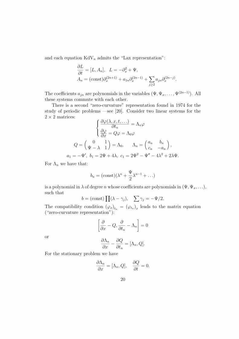
and each equation KdVn admits the “Lax representation”:

∂L

∂t= [L,An], L = −∂2

x + Ψ,

An = (const)∂(2n+1)x + a1n∂(2n−1)

x +∑

j≥2

ajn∂(2n−j)x .

The coefficients ajn are polynomials in the variables (Ψ, Ψx, . . . , Ψ(2n−1)). All

these systems commute with each other.There is a second “zero-curvature” representation found in 1974 for the

study of periodic problems —see [20]. Consider two linear systems for the2 × 2 matrices:

∂ϕ(λ, x, t, . . .)∂tn

= Λnϕ

∂ϕ∂x = Qϕ = Λ0ϕ

Q =(

0 1Ψ − λ 1

)

= Λ0, Λn =(

an bn

cn −an

)

,

a1 = −Ψ′, b1 = 2Ψ + 4λ, c1 = 2Ψ2 − Ψ′′ − 4λ2 + 2λΨ.

For Λn we have that:

bn = (const)(λn +Ψ

2λn−1 + . . .)

is a polynomial in λ of degree n whose coefficients are polynomials in (Ψ, Ψx, . . .),such that

b = (const)∏

(λ − γj),∑

γj = −Ψ/2.

The compatibility condition (ϕx)tn= (ϕtn)x leads to the matrix equation

(“zero-curvature representation”):[

∂

∂x− Q,

∂

∂tn− Λn

]

= 0

or∂Λn

∂x− ∂Q

∂tn= [Λn, Q].

For the stationary problem we have

∂Λn

∂x= [Λn, Q],

∂Q

∂t= 0.

20

Therefore we have the so-called “λ-representation” for the stationary systemwhich is polynomial in λ.

The algebraic curve

Γ = det(Λn(λ) − µ1) = 0

has the formµ2 = R2n+1(λ) = (const)λ2n+1 + · · · .

The stationary generic real solutions are the finite-gap potentials. They areperiodic or quasi-periodic in the generic case.

The hyperelliptic complex curve Γ determines completely the spectrumof the Schrodinger operator L = −∂2

x +Ψ with periodic potential Ψ acting onthe space L2(R). This means exactly that the family of periodic finite-gapSchrodinger operators with given spectrum may be identified with the realpart of the Jacobian variety of the algebraic curve Γ.

The general stationary system for the KdV hierarchy is obtained as alinear combination of the “higher KdV’s”:

Λ = Λn + cnΛn−1 + . . . + cnΛ0,∂Λ

∂x= [Λ, Q].

The last equation describes the set of all n-gap potentials (their Bloch-Floquet eigenfunction is meromorphic on the Riemann surphace with genusg = n ). The Bloch-Floquet eigenfunction is by definition a solution of theequation

Lϕ = λϕ , L = −∂2x + Ψ

such thatϕ(x + T, λ) = exp(ip(λ)T )ϕ(x, λ)

ifΨ(x + T ) = Ψ(x).

For the quasi-periodic potentials Ψ(x) the Bloch-Floquet eigenfunction issuch that the function χ

χ(x, λ) =∂

∂x(log ϕ)

is quasi-periodic with the same periods as the potential Ψ(x). For realbounded smooth potentials all branching points are real and coincide exactly

21

with the endpoints of the spectrum of the operator L acting on the spaceL2(R). People use the expression “finite-gap potentials” in this case, thoughthe expression “algebro-geometric potentials” would probably be more suit-able. The Θ-functional formula can be written in the following very simpleform (found by A. Its and V. Matveev in 1975):

Ψ(x, t1, t2, . . .) = const − 2∂2x log Θ(~U0x +

∑

~Ujtj + ~V0).

Here the Θ-function and the vectors

~Uj = (Uj1 , . . . , Ujn), j ≥ 0

are completely determined by the algebraic curve Γ. The initial phase ~U0

corresponds to the divisor of the poles γ1, . . . , γn.The Bloch-Floquet eigenfunction of a periodic real smooth potential has

the following analytical properties:1) It is meromorphic away from ∞ on the hyperelliptic algebraic curve

Γ =

µ2 = R2n+1(λ) =∏

(λ − λj)

with the real branching points λj

λ0 < λ1 < . . . < λ2n

which are exactly the endpoints of the spectrum in L2(R).2) It has exactly g poles, g = n,

γ1, . . . , γn ∈ Γ

whose projections on the λ-plane C are inside the finite gaps:

λ2j−1 ≤ p(γj) ≤ λ2j, j = 1, 2, . . . , n.

3) It has exponential asymptotics for λ → ∞ of the form

ϕ ∼ exp(

∑

tjk2j+1

)

(1 + O(k−1)), k2 = λ, t0 = x, t1 = t.

22

Lecture 4

Poisson Structures on Loop Spaces.Systems of Hydrodynamic Type and Differential Geometry.

We are going to consider now “local” infinite-dimensional systems. Thephase space M = Map(S1 → Y ) consists of all C∞ maps of the circle intosome C∞ manifold Y with local coordinates (u1, . . . , uN), N =dimY , u(x) =(up(x)), p = 1, . . . , N , x ∈ S1.

The coordinate x here is periodic by definition. It is convenient to forgetnow about the boundary conditions for the formal investigations. All ourconstructions will be local in the variable x. In fact we shall work only with“local” functionals of the following type:

I =∫

S1

j(u(x), u′(x), . . . , u(m)(x), x)dx,

whose density depends on a finite number of derivatives of u at the samepoint x. Its variation

δI =∫ δI

δup(x)δup(x)dx

determines the “Euler-Lagrange” expression of the “variational derivative”

δI/δup(x) ,

which has the form

δI

δup(x)=

∂j

∂up −(

∂j

∂upx

)

x

+ . . . + (−1)m

(

∂j

∂up(m)x...x

)(m)

x...x

.

The pair (p, x) is the right ∞-dimensional analogue of the “index” p: insteadof summation

∑

we shall have∑

p

∫

(. . .)dx in the formulas.Definition. A local Poisson Bracket (PB) of order κ on the space M =Map(S1 → Y ) is given by the formal expression

up(x), uq(y) = ωpq(x, y) =m∑

k=0

bpqk (u, u′, . . . , u(lk), x)δ(k)(x − y).

23

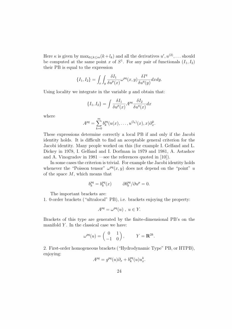
Here κ is given by max0≤k≤m(k+ lk) and all the derivatives u′, u(2), . . . shouldbe computed at the same point x of S1. For any pair of functionals (I1, I2)their PB is equal to the expression

I1, I2 =∫

x

∫

y

δI1

δup(x)ωpq(x, y)

δIq

δuq(y)dxdy.

Using locality we integrate in the variable y and obtain that:

I1, I2 =∫ δI1

δup(x)Apq δI2

δuq(x)dx

where

Apq =m∑

k=0

bpqk (u(x), . . . , u(lk)(x), x)∂k

x .

These expressions determine correctly a local PB if and only if the Jacobiidentity holds. It is difficult to find an acceptable general criterion for theJacobi identity. Many people worked on this (for example I. Gelfand and L.Dickey in 1978, I. Gelfand and I. Dorfman in 1979 and 1981, A. Astashovand A. Vinogradov in 1981 —see the references quoted in [10]).

In some cases the criterion is trivial. For example the Jacobi identity holdswhenever the “Poisson tensor” ωpq(x, y) does not depend on the “point” uof the space M , which means that

bpqk = bpq

k (x) ∂bpqk /∂up = 0.

The important brackets are:1. 0-order brackets (“ultralocal” PB), i.e. brackets enjoying the property:

Apq = ωpq(u) , u ∈ Y.

Brackets of this type are generated by the finite-dimensional PB’s on themanifold Y . In the classical case we have:

ωpq(u) =(

0 1−1 0

)

, Y = R2k.

2. First-order homogeneous brackets (“Hydrodynamic Type” PB, or HTPB),enjoying:

Apq = gpq(u)∂x + bpqk (u)uk

x.

24

The simplest case is Y = R. We have here the so-called “Gardner-Zakharov-Faddeev” (or, briefly, GZF) bracket:

u(x), u(y) = δ′(x − y) , A = ∂x.

The functional I−1 =∫

udx belongs to the annihilator of the GZF bracket.The generalized GZF bracket is by definition the following one:

up(x), uq(y) = gpq0 δ′(x − y),

gqp0 = gpq

0 = (const), Apq = gpq0 ∂x.

All the Hamiltonian systems generated by the Poisson brackets in exam havethe form

∂up

∂t= Apq δH

δuq(x)

for any Hamiltonian H. For example, all the systems of the KdV hierarchyhave the following “Gardner form”:

ut = ∂x

(

δHn

δu(x)

)

, Hn = In.

For n = 0, 1 we have:

n = 0 : ut = ∂x

(

δI0

δu(x)

)

, I0 = (const)∫

u2dx,

n = 1 : ut = ∂x

(

δI1

δu(x)

)

, I1 = (const)∫

(

u2x

2+ u3

)

dx.

Let us give the general description of the functionals Hn: consider the formalsolution of the Riccati equation:

χ(x, k) = k +∑

m≥1

χm/(2k)m,

χ′ + χ2 = u − λ, k2 = λ.

For m = 2k + 1 we have∫

χ1dx = (const)∫

udx = I−1,

25

∫

χ3dx = (const)∫

u2dx = I0,∫

χ5dx = (const)∫

(u2x/2 + u3)dx = I1

· · ·∫

χ2k+3dx = (const)Ik.

3. There is a very interesting “Lenard-Magri bracket” defined by:

u(x), u(y) = cδ(3)(x − y) + 2u(x)δ′ + u′δ,

A = c∂3x + u∂x + ∂xu.

This PB has no local annihilator. It gives us also the Hamiltonian form forthe KdV hierarchy but with a “shift” of the Hamiltonians (c = 1):

KdV0 : ut = ux = A(δI−1/δu(x)),

KdV1 : ut = 6uux − uxxx = A(δI0/δu(x)),

· · ·KdVn : ut = (const)u(2n+1) + . . . = A(δIn−1/δu(x)).

Now, going back to the beginning of the lecture, we generalize the situa-tion by considering M = Map(T n → Y ), the space of smooth functions u(x)from the n-torus to an N -dimensional manifold Y . We have x = (x1, . . . , xn)and locally u = (u1, . . . , uN).Definition. We call Hydrodinamic (or Riemann) Type (or, briefly, HT)equation an equation having the following form in local coordinates:

upt = V p,α

q (u(x))uqα.

Here the coefficients V p,αq define the “velocity” tensor fields V α , α = 1, . . . , n,

V = V pq (u), on the manifold Y .

The main problems which we will discuss are the following:

1. How can we construct the local Hamiltonian formalism for HT Systems?

2. How can we find HT systems which are completely integrable? Arethe natural HT systems (which already appeared in the description ofthe “slow modulation of parameters” in the so-called Whitham method—i.e. in the “non-linear analogue of WKB-asymptotics” for KdV, SG,NS) completely integrable?

26

Problem 1 was solved in 1983 in a joint work of B. Dubrovin and the au-thor; problem 2 was solved by S. Tsarev in 1985 on the base of Hamiltonianformalism —see [10]. We will explain here some ideas used in the solutionof these problems. The applications to soliton theory will be discussed inLecture 5.Definition. We call Riemann Invariants (or, briefly, RI) coordinates (u1, . . . , uN )on the target manifold Y with the property that all the velocity tensors V α

are diagonal:

V α = V p,αq (u) = V p,α(u)δp

q α = 1, . . . , n.

According to a classical result (of Riemann) we have that for n = 1 andN = 2 RI always exist. For N ≥ 3 they do not exist in general (even forn = 1). In case N = 2 and n = 1 the HT equation is linear in the inversefunctions

x(u1, u2) , t(u1, u2).

The map (x, t) 7→ (u1, u2) is the “hodograf transformation”; it is quite naturalto ask whether there exists any analogue of the “hodograf” for n = 1 andN ≥ 3. Such an analogue has been found by Tsarev for Hamiltonian systems.Definition. The functional H =

∫

h(u)dx is called a functional of Hydrody-namic Type (or, briefly, HT) if its density does not depend on the derivativesux, uxx, etc.Definition. We call Hydrodynamic Type Poisson Bracket (or, briefly, HTPB)a bracket having the form

up(x), uq(y) = gpq,α(u(x))δα(x − y) + bpq,αk (u(x))uk

αδ(x − y),

Apq = gpq,α∂kα + bpq,α

k ukα.

Here ∂α = ∂/∂xα, ukα = ∂uk/∂xα, δα = ∂δ/∂xα. (We will use the symbol ∂α

with the meaning of ∂/∂xα only with Greek subscripts α, while in the sequelwe will use ∂k, with Latin subscripts k, to denote the local derivative ∂/∂uk

on Y .)The HT Hamiltonians generate the HT equations through the HTPB’s:

H =∫

h(u)dnx, upt = V p,α

q (u)uqα,

V p,αq (u) = gps 5(α)

s 5(α)q h(u),

27

(but 5(α)q h(u) = ∂qh(u) because h(u) is a scalar). For the covector fields we

define:5(α)

p Xq = ∂pXq − Γs,αpq Xs, bpq,α

k = Γq,αsk gps,α.

Theorem 1 ([9]). Let det(gpq,α) 6= 0 for α = 1, . . . , n. The collection ofcoefficients of the Hydrodynamic Type PB transforms in the following way:the coefficients gpq,α as components of a tensor of rank 2; the coefficientsΓq,α

sk as Kristoffel symbols. The tensors (gpq,α) are symmetric. The covariant

derivative 5(α)k gpq,α is zero. Torsion and Curvature of the connection (Γpq,α

k )are zero.Corollary. If n = 1 there exists a system of “flat” coordinates (u1, . . . , uN)such that

gpq = gpq0 = const, bpq

k = 0.

The signature of the metric gpq(u) is a complete local invariant of the HTPBif det(gpq)(u) 6= 0. Therefore the covariant derivatives commute with eachother in any coordinates:

5p5q = 5q 5p .

For the velocity tensor of a Hamiltonian HT system we have:

Vpq = gpsVsq = Vqp = 5p 5q h(u) = 5q 5p h(u) (gpsg

sq = δqp)

(it is a symmetric tensor).Theorem 2. Let n > 1 and det(gpq,1) 6= 0. In the coordinates (u1, . . . , uN)which are flat for the metric (gpq,1) we have:

gpq,α = Cpq,αk uk + const, Cpq,α

k = const,

bpq,αk = const, α ≥ 2, Cpq,α

k = bpq,αk + bqp,α

k , (bpq,1k = 0).

(This result was proved by Dubrovin and the author in 1984 for N ≥ 3 andby Mokhov (later) for N = 2; some mistakes of the original proof for N ≥ 3were fixed by Mokhov in 1988 —see [10] and the references quoted therein.)Remark. The case of a HTPB when the tensor (gpq) is singular and hasconstant rank has also been investigated. The kernels of the metric (gpq)generate an integrable foliation on the manifold Y with interesting geometricstructures which have never been completely classified. A very interestingproblem is also to investigate the generic singularities of a HTPB when therank of (gpq) is not a constant.

28

Examples.1. Flat coordinates gpq = gpq

0 , det(gpq) 6= 0. Our bracket is exactly thegeneralized GZF bracket. The standard GZF bracket δ′ has HT but theKdV Hamiltonian does not have HT. The second LM bracket does not haveHT, but the LM Hamiltonian for KdV has HT.2. For the Lie algebra L(n) of the vector fields in T n (or Rn) we have

[V,W ]p = (∂kVp)W k − (∂kW

p)V k.

Here N = n. The corresponding Lie-Poisson bracket has the following form:

pα(x), pβ(y) = pα(x)δβ(x − y) − pβ(y)δα(y − x)

= pα(x)δβ(x − y) + pβ(y)δα(x − y).

The variables pα describe the adjoint space L∗n. They are such that the

expression:∫

pα(x)V α(x)dnx

is invariant under changes of coordinates x = x(x′). Therefore the objects(pα) transform like the components of the density of a covector (“density ofmomentum” in HT theory).

In the hydrodynamic of a compressible liquid (without viscosity) we havetwo more fields:

ρ (density of mass), M =∫

ρ(x)dnx,

s (density of entropy), S =∫

s(x)dnx,

with PB:

pα(x), ρ(y) = ρ(x)∂αδ(x − y),

pα(x), s(y) = s(x)∂αδ(x − y),

ρ, ρ = s, s = ρ, s = 0.

The Hamiltonian has the standard form:

H = “energy” =∫

[

p2

2ρ+ ε0(ρ, s)

]

dnx, p2 =n∑

α=1

p2α.

29

By definition we have (as “velocities”):

Vα = pα/ρ.

The functionals M =∫

ρdx, S =∫

sdx, ~P =∫

~pdx belong to annihilator .Other interesting examples can be found in [21], Section 2, e.g. the su-

perfluid liquid.For n = 1 we have:

p(x), p(y) = [p(x) + p(y)]δ′(x − y) = 2p(x)δ′(x − y) + p′(x)δ(x − y).

After the change of the function p = u2 we are coming to the standard formof the GZF bracket:

u(x), u(y) = (const)δ′(x − y).

The “Lenard-Magri bracket”:

p(x), p(y) = cδ(3)(x − y) + 2p(x)δ′(x − y) + p′(x)δ(x − y)

is therefore a central extension of the Lie-Poisson Bracket associated withthe Lie algebra of vector fields on the circle S1 (we are considering n = 1).It corresponds to the central extension of this algebra by the third order“Gelfand-Fucks cocycle” (see below). Therefore the LM bracket correspondsto the “Virasoro algebra” (Virasoro-Gelfand-Fucks-Bott: in fact the Virasoroalgebra is a subalgebra of this one generated by the trigonometric polynomi-als):

[V,W ] = V ′W − W ′V + χ(V,W )t, [t, V ] = 0,

χ(V,W ) =∮

S1

V (3)(x)W (x)dx, V = V (x)∂x, W = W (x)∂x.

The general first-order translationally invariant Lie algebra structure on thespace of C∞-vector functions on the circle S1 with values in the space RN = Ymay be described in the following way: consider a basis e1, . . . , eN of RN anda bilinear multiplication determined by structural constants

ep eq = bpqk ek.

We have an algebra B (which is RN as a set).

30

Lemma. The operation [ , ] on the space M = Map(S1 → B) = LB definedas

[P,Q](x) = P ′ Q − Q′ P

for P = fp(x)ep and Q = gp(x)ep ∈ B, satisfies the Jacobi identity if andonly if for any three elements a, b, c of B we have

a(bc) = b(ac) , [Lb, La] = 0, R[bc−cb] = [Rb, Rc].

By definition, the left and right multiplication operators are:

La(b) = Rb(a) = a b.

Remarks.1. The (equivalent) facts of the previous Lemma are true in particular if B isa commutative associative algebra. (Remark that if B is commutative thenit is also associative, but not conversely. Moreover if B has a unit then it isautomatically commutative and associative.)2. The algebra B which corresponds to the HTPB of a compressible liquid(n = 1) is 3-dimensional (generated by the fields p, ρ, s), non-commutativebut associative. There are 3 basic elements:

e (corresponding to p), f (corresponding to ρ), g (corresponding to s)

and e is a left unit; we have

e a = a, a ∈ B, f B = g B = 0.

3. E. Zelmanov proved in 1987 that the finite-dimensional algebras B arenever simple if N =dimB > 1 for characteristic 0 (see [10]). They maybe simple for N = ∞ or for fields of positive characteristic. There arevery interesting examples constructed recently by Osborn which we shall notdiscuss (see [24]). There is also an “extension theory” for the algebras B (see[3]).

We get a particularly interesting class of examples from classical commu-tative associative “Frobenius algebras” B with unit . In our language theFrobenius property exactly means that:

det(gpq(u0)) 6= 0

31

for the generic point

u0 = (u10, . . . , u

N0 ), gpq = cpq

k uk, cpqk = bpq

k + bqpk = 2bpq

k .

The pseudo-Riemannian metric (gpq(u)) has zero curvature by Theorem 1above. Therefore there exists a system of flat coordinates. How to find it? Inthe Frobenius case it is easy. Fix some point (u0) such that det(gpq(u0)) 6= 0;consider the inverse matrix

g0pqg

qs0 = δs

p

and the corresponding Kristoffel symbols at u0:

F pqk = Γp

qk(u0) = g0qsb

psk = F p

kq

(they are symmetric because the torsion is equal to zero by Theorem 1 again).The quadratic trasformation

up = F pqkv

qvk

introduces a flat coordinate system (v1, . . . , vN) (cfr. [3]). For N = 1 we haveu = v2 (as above). Such a transformation is unknown for general B-algebras.

A very interesting problem is to classify the central extensions of the Liealgebras LB:

O → R → LB → LB → 0.

Especially interesting are local translationally invariant extensions of orderτ = 0, 1, 2, 3 written in the form

χ(P,Q) =∮

S1

f (τ)p Gqγ

pqdx, γpq = const = (−1)τ+1γqp.

For τ = 3 we have the “Gelfand-Fucks” type cocycles. In the Frobenius casethe group of “central extesions”

H2(LB,R)

contains many non-trivial non-degenerate cocycles of order τ = 3:

γpq = Gpq(u0).

(No proof has been published, but Balinsky claimed in his Ph.D. thesis thatthe group H2(LB,R) contains in this case these cohomology classes only.)

32

For τ = 1 the cocycles γpq are such that the “perturbed” metric tensor

gpq(u) = gpq(u) + εγpq = cpqk uk + εγpq

determines a new HTPB with the same (bpqk ).

For the PB of a compressible liquid we have (n = 1, N = 3) and

det(gpq(u)) ≡ 0

but there is a cocycle γpq of order τ = 1 such that

det(gpq(u) + εγpq) 6= 0

at the generic point u0.Non-degenerate cocycles of order τ = 2 might be very interesting.

We have different types of important coordinate structures associatedwith HTPB’s:

• flat coordinates;

• Riemann Invariants;

• Lie algebra structures (linear coordinates);

• Physical Coordinates (to be defined).

We are going to introduce now the notion of “Physical Coordinates” or“Liouville” coordinates, which are important in soliton theory.Definition. Let a HTPB be given by the tensor (gpq(u)) and the quantities(bpq

k (u)), written in the following Liouville form: there exists a tensor fieldγpq(u) such that

gpq(u) = γpq(u) + γqp(u), bpqk (u) =

∂γpq(u)

∂uk ;

coordinates (u) enjoying this property will be called Liouville or Physicalones.Remarks.

33

1. Obviously for any Lie algebra the natural linear coordinates are Liouvilleones because we may define:

γpq = bpqk uk.

2. For the Liouville coordinates (u) any affine transformation

vp = Apqu

q + vp0

defines new Liouville coordinates. Therefore the Liouville coordinates deter-mine an “affine structure” on the target manifold Y .Definition. The Liouville structure is called strong if the restriction of thetensor γpq(u) to some subset of coordinates (up1 , . . . , upk) determines a well-defined Liouville structure on the subspace Y ⊂ Y corresponding to such aset of coordinates.

This property should hold for any coordinates (v) obtained from (u) byaffine transformation.Remark. For N = 3 it is easy to check that the HTPB of a compressibleliquid (see above) is written in the strongly Liouville form; the PhysicalCoordinates (p, ρ, s) in this case satisfy to the additional requirement.

The present author and B. Dubrovin made a mistake in the proof of The-orem 1 of Section 6 in [10]: the HTPB in the Physical coordinates is onlyLiouville, not strong. The paper of the present author in collaboration withthe student Maltsev correcting this mistake will appear in Uspechi Math. Nauk(1993) issue 1 (January-February).

Probably very few linear HTPB’s (i.e. Lie algebras) have tensors whichare strongly Liouville. It is the author’s opinion that it should be possible toclassify all of them.

The role of Physical Coordinates will be clarified in Lecture 5.We are coming now to the “integration theory” for Hamiltonian HT sys-

tems developed by S. Tsarev in his Ph.D. thesis in 1985. It was alreadyknown for many years that some HT systems which appear in the KdV the-ory through the so-called “Whitham method” (i.e. the “non-linear WKBmethod”) admit Riemann Invariants (G. Whitham in 1973 for n = 1 andN = 3; H. Flashka, G. Forest and D. McLaughlin in 1980 for N = 2m + 1and n = 1).

The differential-geometric Hamiltonian formalism (above) for these HTsystems was developed by B. Dubrovin and the author in 1983; later the

34

author formulated the following conjecture: in the class of Hamiltonian HTsystems existence of Riemann Invariants automatically implies complete in-tegrability. This conjecture has been proved by S. Tsarev in his remarkablepaper [25].

We are going to explain now some ideas of Tsarev’s work. Consider anyHT system which is written in its Riemanian Invariants (r1, . . . , rN ) as:

∂rk

∂t= V k(r(x))

∂rk

∂x(no summation!).

Suppose we are dealing with the Hamiltonian system corresponding to thelocal Hamiltonian formalism developed above, and that in the generic pointwe have:

V k(r) 6= V l(r), k 6= l, det(gkl(r)) 6= 0.

It is easy to check the corresponding property of the metric tensor:

gkl(r) = gk(r)δkl

(i.e. the tensor is diagonal). Therefore the Riemann Invariants are orthogonalcoordinates for the pseudo-Riemannian metric (gkl) on the target manifoldY , which generates the Hamiltonian formalism. The main result is:Lemma. For any HT system for which the coordinates (r1, . . . , rN) areRiemann Invariants, i.e.

∂rk

∂t= W k(r(x))

∂rk

∂x(no summation!)

the following indentity is true:

∂iWk

Wi − Wk

= Γkki, i 6= k.

All these systems commute (in fact all of them are HT Hamiltonian systemsgenerated by the same HTPB).

The last equation might be considered as an equation for finding all theHT flows commuting with each other, provided the symbols Γk

ki are known.In particular we have for any diagonal metric:

Γkki = ∂i log |gk(r)|1/2, gk = 1/gk(r).

35

As a consequence we have

∂i

(

∂jWk

Wj − Wk

)

= ∂j

(

∂iWk

Wi − Wk

)

, i 6= j 6= k.

Definition. Any diagonal HT system (written in its RI) is called semi-Hamiltonian if the last equation is true for the velocities Wk(r). (We actuallyhave that all such systems being not Hamiltonian in the HTPB above arein fact Hamiltonian systems corresponding to some non-local Hamiltonianformalism generalizing the HTPB above, for which the metric is diagonalbut some components of the curvature tensor may be non-zero. This factwas recently observed by Ferapontov, in 1990.)Theorem 3. A. The solutions of the system

∂iWk

Wi − Wk

= Γkki

give the commuting family of HT systems which is enough for Liouville in-tegrability (of course this is a local differential-geometric statement). Thestatement is globally true if all the initial functions rk(x, 0) are convex (theseflows generate the tangent space to the common level of the commuting in-tegrals).B. For any commuting pair of such systems

∂rk

∂t= Vk(r)

∂rk

∂x,

∂rk

∂τ= Wk(r)

∂rk

∂τ

the solution (rk(x, t)) of the equation

Wk(r) = Vk(r)t + x, k = 1, . . . , N, (rk = rk(x, t))

satisfies the first system.(For the proof see [10].)There are some very special classes of systems (called “weakly non-linear”)

found by S. Tsarev and M. Pavlov for which the construction of the abovetheorem may be realized directly. But our systems do not belong to theseclasses.

Using the Hamiltonian formalism we can construct families of solutionsonly if we know many HT integrals; we shall use this technique, but the

36

natural integrals which we actually know do not give a complete family.The differential-geometric procedure of Tsarev is therefore not sufficientlyeffective. In the study of concrete important really non-trivial integrable HTsystems we shall use the additional algebraic-geometric information aboutthis HT system (see Lecture 5). For KdV all this problems have been quiterecently solved by several people, among which Krichever, Potemin, Tian,Dubrovin and Krylov. We will present here only special results about veryspecial important solutions (see Lecture 5), based on the results of Kricheverand Potemin of 1989.

The latest results of other authors may be found in the transactions ofthe Conference dedicated to this subject held in Lyon in July 1991, whichare going to be published soon.

37

Lecture 5

Non-linear WKB (Hydrodynamicsof Weakly Deformed Solution Lattices).

Consider an evolutional system of non-linear differential equations

Ψt = K(Ψ, Ψx, Ψxx, . . .)

where K is a polynomial with constant coefficients in the variables (Ψ, Ψx, . . .).Here Ψ may be a vector function. The simplest “hydrodynamic” approxi-mation we get is for the class of very slowly varying functions, i.e. functionssuch that each derivative is much smaller then the previous one:

Ψ(n) << Ψ(n−1) << Ψ(n−2) << . . . << Ψ.

It is convenient to introduce an algebraic “filtration” with the properties

f(Ψ) ≥ 0, f(Ψ(k)) ≥ k, f(AB) ≥ f(A) + f(B).

For the equation we get the decomposition

Ψt = K0(Ψ) + K1(Ψ)Ψx + . . .

where the remaining terms have filtration at least 2. Suppose all Ψ = constare exact solutions. In this case K0(Ψ) = 0.

We are coming to the HT system as the first hydrodynamic type ap-proximation to the original system for the class of “very smooth” functionsΨ(X,T ), X = εx, T = εt (slow modulations of the constant solutions):

ΨT = K1(Ψ)ΨX .

This remark is trivial (but very useful). A much more profound “non-linearWKB method” has been developed by Whitham in 1965.

Suppose that we already know a family of exact periodic (or quasi-periodic) solutions

Ψ(x, t) = F (~Ux + ~V t + ~U0, u1, . . . , uN )

38

depending on the N parameters u1, . . . , uN . Here the vectors U and V (notU0) should be already known as given functions of the parameters:

Uk(u1, . . . , uN ), Vk(u

1, . . . , uN ), k = 1, . . . ,m.

The initial phase ~U0 may be an arbitrary m-vector. The function F shouldbe periodic with period 2π in each of the first m variables:

F = F (η1, . . . , ηm, u1, . . . uN) ηj(η1, . . . , ηm) ∈ T m.

For any (u = const) we get an exact solution of the original system (“m-phase solution”). For m = 0 we get constants (provided Ψ = const satisfiesthe original equation). The most popular case is m = 1 which is sufficientlynon-trivial. Many systems have families of periodic solutions as “travelingwaves”:

x = Uη + U0, Ψ(x − ct), Ψ(η + T ) = Ψ(η).

For integrable systems like KdV, SG and NS there exist very large fami-lies of m-phase quasi-periodic solutions (“finite-gap” or “algebro-geometric”solutions).

M. Ablowitz and D. Benney discussed in 1970 the “m-phase” analogue ofG. Whitham’s method (who developed it for m = 1 only) but there was noconcrete base for serious development because the family of m-gap solutionswas found for the first time in 1974.

Serious analogues of Whitham’s theory for the cases m > 1 started in thelate seventies only; they are due to H. Flashka, G. Forest, D. McLaughlin,Dobrokhotov and V. Maslov.

Suppose now that the parameters (u1, . . . , uN) are not constants but only“slow functions”:

up = up(X,T ), X = εx, T = εt.

Consider a vector-function

(S1, . . . , Sm) = S(X,T )

such that∂Sj/∂X = Uj(u), ∂Sj/∂T = Vj(u).

39

Let us consider the following question: is it possible to find the smooth func-tions (up) in such a way that the expression:

Ψ = F (S(X,T ), u1(X,T ), . . . , uN (X,T ))

satisfies the original evolutional equation asymptotically? This fact means bydefinition that

Ψt = K(Ψ, Ψx, . . .) + o(1) for ε → 0.

This question has been investigated well enough for the case m = 1 only, butthe formal procedure is valid for m > 1 as well.

For non-degenerate Lagrangian systems the question was first faced byby G. Whitham in 1965, J. Luke in 1966, V. Maslov in 1969, Hayes in 1973and others (see [8] and the references quoted therein). The main resultis that there exists a collection of “velocity coefficients” V p

q (u) such thatthe following HT system gives the necessary condition for the expressionΨ = F (S, u(X,T )) to be an asymptotic solution of the original equationΨt = K:

upT = V p

q (u(X,T ))uqT .

The velocity coefficients were constructed for KdV also by Whitham form = 1 and by Forest, Flashka and McLaughlin for m > 1. These systemsadmit Riemann Invariants for KdV, NS, SG.

Are these HT systems Hamiltonian? We can consider this problem in amore general form. Assume the original system is Hamiltonian, correspond-ing to some PB which is local and translationally invariant:

Ψl(x), Ψi(y)0 =m∑

k=0

Blik (Ψ, Ψx, . . .)δ

(k)(x − y),

I1 = H =∫

i1(Ψ, Ψx, . . .)dx.

Suppose that there exists a collection of N local integrals H = I1, . . . , In:

Ik =∫

Jk(Ψ, Ψx, . . .)dx

and a family of exact quasi-periodic solutions (on the tori T m(u))

Ψ = F (Ux + V t + U0; u1, . . . , uN)

such that:

40

1. the integrals are in involution, i.e. Ik, Il0 = 0;

2. the family of exact solutions Ψ = F satisfies all the conditions above.This family is invariant under the flows generated by the integrals Ik.The restriction of these integrals to the family transforms it in thefamily of finite-dimensional completely integrable systems. This familyshould be non-degenerate in the sense that the components of the vectorU generate the ring of functions in the variables u with trascendencydegree equal to m. The number N should be equal to 2m + a where ais the number of integrals Ik who belong to the local annihilator of theoriginal field-theoretical PB;

3. the averaged densities coincide exactly with the parameters u above:

Jk(Ψ, Ψx, . . .) = uk

(any function of the variables (Ψ, Ψx, . . .) might be averaged on thetori, as Ψ, Ψx, . . . vary on the tori).

Consider now the PB’s of the densities:

jk(Ψ(x), . . .), jl(Ψ(y), . . .)= Akl

0 (Ψ(x), . . .)δ(x − y) + Akl0 (ϕ(x), . . .)δ

′

(x − y) + · · · .

As a consequence of the involutivity condition∫

jkdx,∫

jldy

= 0

we have

Akl0 (ϕ(x), . . .) =

∂

∂xQkl(ϕ(x), ϕ′(x), . . .)

for any smooth function ϕ(x) ∈ C∞(S1).Let us define now

γkl(u) = Qkl

+ (const), gkl(u) = Akl

1 = γkl + γlk.

Theorem 4. A. The coordinates u1, . . . , uN defined above are the Physicalones, which means that our formulas determine a 0-curvature metric in theLiouville form.

41

B. The functionalH =

∫

u1dx , u1 = j1 = h

determines exactly the Whitham equations (“the Hydrodynamic of SolitonLattices” or “the system for slow modulations of the parameters”) when-ever they were constructed before using the HTPB defined by the metric(including the averaged KdV for all m ≥ 1).Remark. For non-degenerate Lagrangian systems and N = 2m it wasproved by Whitham and Hayes that the averaged HT system is also La-grangian. It leads to the new “Clebsh-type” coordinates

(U1, . . . , Um, J1, . . . , Jm) = (W 1, . . . ,W 2m)

with respect to which the HT system has the form:

∂

∂T

Jk = ∂X

(

δH

δUk(X)

)

, ∂T Uk = ∂X

(

δH

δJk(X)

)

.

In this case we are coming to flat coordinates. The HTPB has the form

W p(x),W q(y) = gpq0 (W (x))δ

′

(x − y), gpq0 =

(

0 11 0

)

.

The signature of this metric is (m,m). Our flat coordinates (W ) are suchthat the second group of variables

Jk = Wm+k, k = 1, . . . ,m

exactly coincides with the group of “action variables” (defined above) ofthe finite-dimensional Hamiltonian subsystem of the original system whosesolutions are quasi-periodic and generate the “non-linear WKB method” dis-cussed above.

For KdV we have N = 2m + 1, m ≥ 1 and and the corresponding metrichas signature (m,m + 1). More exactly, the HT systems corresponding tothe KdV equation might be described using two different Hamiltonian struc-tures (GZF and LM) —see Lecture 4. After averaging we get two differentHTPB’s corresponding to these structures; the restriction of the metric tothe variables (U, J) is still the same but they do not give complete systemsof coordinates; the action variables are different for GZF and LM. For GZF

42

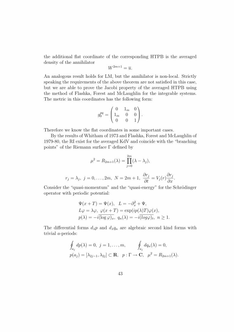
the additional flat coordinate of the corresponding HTPB is the averageddensity of the annihilator

W 2m+1 = u.

An analogous result holds for LM, but the annihilator is non-local. Strictlyspeaking the requirements of the above theorem are not satisfied in this case,but we are able to prove the Jacobi property of the averaged HTPB usingthe method of Flashka, Forest and McLaughlin for the integrable systems.The metric in this coordinates has the following form:

gpq0 =

0 1m 01m 0 00 0 1

.

Therefore we know the flat coordinates in some important cases.By the results of Whitham of 1973 and Flashka, Forest and McLaughlin of

1979-80, the RI exist for the averaged KdV and coincide with the “branchingpoints” of the Riemann surface Γ defined by

µ2 = R2m+1(λ) =2m∏

j=0

(λ − λj),

rj = λj, j = 0, . . . , 2m, N = 2m + 1,∂rj

∂t= Vj(r)

∂rj

∂x.

Consider the “quasi-momentum” and the “quasi-energy” for the Schrodingeroperator with periodic potential:

Ψ(x + T ) = Ψ(x), L = −∂2x + Ψ,

Lϕ = λϕ, ϕ(x + T ) = exp(ip(λ)T )ϕ(x),

p(λ) = −i(log ϕ)x, qn(λ) = −i(logϕ)t, n ≥ 1.

The differential forms dλp and dλqn are algebraic second kind forms withtrivial a-periods:

∮

aj

dp(λ) = 0, j = 1, . . . ,m,∮

aj

dqn(λ) = 0,

p(aj) = [λ2j−1, λ2j] ⊂ R, p : Γ → C, µ2 = R2m+1(λ).

43

The poles of the forms dp and dqn are displaced at the point λ = ∞ andhave the asymptotics:

dp = (dk + reg), k2 = λ,

dqn = (dkn + reg), n ≥ 1.

The canonical cycles are such that:

ak bl = δkl, bk bl = 0, ak al = 0.

By definition we have:

Uj =∮

bj

dp(λ), V(n)j =

∮

dqn(λ), p = q0.

The quantity

p(λ) = λ1/2 +∑

s≥0

Is−1

(2λ1/2)2s+1

is in fact the integral from the solution of the Riccati equation (see above):

p(λ) =∫ T

0dx = lim

T→∞

1

T

∫ T

0χ(x)dx = ~χ.

For the velocities of the HT systems generated by the averaged integrals Is

through the HTPB we have the following formulas:

rj = λj , j = 0, 1, . . . , 2n

V(s)j (r) =

(

dqs(λ)

dp(λ)

)

λ=λj

, s ≥ 0.

Here we have (dq0 = dp); the most important property is that:

Vj(αr) = αVj(r).

Through Tsarev’s procedure the averaged integrals Is generate exact solu-tions (“averaged finite-gap” in our terminology). Krichever observed in 1987that these exact solutions are in fact self-similar (see [10]).

44

Consider now the special case m = 1 which is non-trivial and physicallyimportant. We have:

−V0 =

2∑

j=0

rj

/3 − 2

3(r1 − r0)

K

K − E,

−V1 =

2∑

j=0

rj

/3 − 2

3(r1 − r0)

(1 − s2)k

E − (1 − s2)K,

−V2 =

2∑

j=0

rj

/3 − 2

3(r2 − r0)

(1 − s2)K

E,

s2 =r1 − r0

r2 − r0

, 0 ≤ s2 ≤ 1,

V2 ≥ V1 ≥ V0, r2 ≥ r1 ≥ r0.

(K and E are the elliptic integrals —see [4]).The special case r1 = r0 corresponds to a constant solution of KdV. The

case r2 = r1 corresponds to a soliton which is rapidly descreasing . Thegeneric “knoidal wave” has the form for KdV

u(x, t) = 2P(x − ct) + const

(P is a Weierstrass elliptic function corresponding to the algebraic curve Γ ofgenus g = m = 1). The generic solution generated by the averaged Kruskalintegrals Is has velocities written in the form:

∑

s≥0

asIs 7→

Wj(r) =∑

s≥0

asW(s)j (r)

, W(s)j (r) =

(

dqs(λ)

dp(λ)

)

λ=λj

.

Following Tsarev’s procedure we have to solve the equation

Wj(r) = Vj(r)T + X,

rk = r(x, t), k = 0, . . . , N − 1, N = 2m + 1.

For the basic Kruskal Integrals

cs = 1 , ci = 0 , i 6= s

45

we obtain special self-similar solutions:

rk(X,T ) = T γRk(XT−1−γ), γ =1

s − 2(s 6= 2).

For s = 4 and γ = 1/2 we obtain a solution which G. Potemin identified (inhis Ph.D. thesis) with the very important “dispersive analogue of the shockwave” defined by A. Gurevitch and L. Pitaevski in 1973 —see the referencequoted in [10].

In this case we have:

Wk =1

35[(3Vk − a)fk + f ], f = 5a3 − 12ab + c,

a =∑

rj, b =∑

i≤j−1

rirj, c = r0r1r2, fi =∂f

∂ri

, i = 0, 1, 2.

This solution is defined on the interval

4 : −√

2 ≤ z ≤√

10

27, z = XT−3/2, γ = 1/2.

Outside the interval 4 this solution should be continued as the multi-valuedC1-function R(z) such that:

z + R/T = R3 (z 6∈ 4), R = r/√

T ,

R(

−√

2)

= R2

(

−√

2)

, R1

(

−√

2)

= R0

(

−√

2)

,

R

(√

10

27

)

= R0

(√

10

27

)

, R2

(√

10

27

)

= R1

(√

10

27

)

.

Outside the interval 4 we use the trivial Hopf equation (“variation of con-stants”)

x + 6rt = r3, rt = 6rrx.

Inside 4 we use the non-linear WKB method with m = 1.The dispersive analogue of the shock wave appears in the following way.

Let us start from the “very smooth” initial data for KdV and approximatethe equation by the trivial one:

Ψt = 6ΨΨx, Ψx << Ψ, Ψxx << Ψx, · · · .

46

After some development we find that the first derivative Ψx tends to ∞ ast → t0 and x → x0; hence the trivial approximation does not work for “theshock wave situation”, which may be locally approximated by a cubic curve.Some “Oscillation Zone” (briefly, OZ) for the original KdV equation appearsin this case, and we shall see no discontinuities at all for any time.

Inside this OZ the non-linear WKB method works for large t; outside itwe continue to use the trivial Hopf equation for any time. On the boundaryof the OZ we have

OZ = [x−(t), x+(t)],

r(x−) = r1(x−) = r0(x−) < r2(x−),

r(x+) = r2(x+) = r1(x+) > r0(x+).

For x < x− and x > x+ we use the trivial Hopf equation for r(x, t). It wuoldbe important to find some equation for the boundary of OZ

dx−

dt=? ,

dx+

dt=?

The multi-valued function r(x, t) (which is single-valued for x < x(t) andfor x > x+(t)) should be at least C1 everywhere and satisfy the followingasymptotic conditions for x → x±(t):

r = r(x, t), if x > x+, x < x−; r = (r0, r1, r2), if x ∈ [x−, x+];

r0 = r1 at x = x−, r1 = r2at x = x+;

r(x, t) of class C2 near x−(t), x ∈ 4;

0 < x − x− = a−(r − r−)2 + o(r − r−)2;

0 > x − x+ = a+f(1 − s2) + o(r − r−)2;

f(u) = u log(

16

u+ 1/2

)

, u = 1 − s2.

These conditions are discussed in [2], where also the following equations forx±(t) were found:

x+ = V +1 = V +

2 , r+ = −|r+2 − r+

1 |/12a+;

x− = V −0 = V −

1 , r− = −1/2a−;

47

r+ = r+2 = r+

1 , r− = r−0 = r−1 .

The self-similar solution of Gurevitch and Pitaevski (found in 1973) has nosingularities inside 4 (as Potemin proved in 1988-90); therefore it satisfiesour requirements. The C1-property was first missed and then proved in 1990;by definition the interval 4 is constant in the coordinate z

z = xt−1/2.

For the function r(x, t) we have

r(x, t) → x1/3, x → ±∞

because r = Ψ outside 4. This fact means that the length of 4 is smallenough (and we may use the cubic form of the curve which in fact is a localobject). The author’s numerical investigation (carried out in 1987) confirmedthat the Gurevitch-Pitaevski dispersive shock wave is a stable solution of ourproblem, and it is asymptotically attractive for an open set of admissiblemulti-valued functions r(x, t).

This numerical result has been proved and extended to a very large openset by Tian and others in 1991 on the basis of the exact analytic solution ofthe problem using the methods described above.

The influence of the small viscosity on the situation above has been inves-tigated in 1987 by the author in collaboration with V. Avilov and Krichever(and also by L. Pitaevski and A. Gurevitch —see in [10]).

The foundation of the averaging (non-linear WKB) method for the Kd-Vsystem with small dispersion term

Ψt = 6ΨΨx + δΨxxx , δ → 0

has been investigated by P. Lax and C. Levermore starting from 1983, and byS. Venakides starting from 1987. Some important asymptotic results wereobtained also by R. Its, R. Biklaev and V. Novokshenov, using “isomon-odromic” deformations, in 1983-1989 (see the references in [10]).

References

[1] Arnold V.I., UMN (RMS) , v. 24:3 (1969), 225

48

[2] Avilov, Novikov. 1987.

[3] Balinsky, Novikov. 1985.

[4] Bateman H., Erdelyi A. Higher transcendent functions, McGraw-HillCompany, New York (1955), vol.3.

[5] Bobenko A.UMN (Russ Math Syrveys ) v. 46:4 (1991), 3-42.

[6] Dubrovin B.A., UMN (RMS) v. 36:2 (1981), 11-80.

[7] Dubrovin B.A., Krichever I.M., Novikov S.P. Encyclopedya of Math.Sci,Springer, Dynamical Systems 4, vol. 4 (Arnold V.I., Novikov S.P. edi-tors).

[8] Dubrovin B.A., Matveev V.B., Novikov S.P. UMN (Uspechi Math. Nauk= Russ. Math. Surveys) v. 31:1 (1976), 55-136.

[9] Dubrovin, Novikov. 1983.

[10] Dubrovin B.A., Novikov S.P., UMN (RMS) v. 44:6 (1989), 29-98.

[11] Dubrovin B.A., Novikov S.P., Fomenko A.T. Modern Geometry, v.2,Springer, 1990 (second edition).

[12] Kirillov, article about representation, maybe quoted in [7].

[13] Krichever I.M., UMN (RMS) v. 32:6 (1977), 180-208.

[14] Krichever I.M., Novikov S.P. UMN (RMS), v. 35:6 (1980), 47-68.

[15] Krichever I. M., Novikov S. P., Funk. Anal.Appl, v. 21:2 (1987), 46-63.

[16] Krichever I. M., Novikov S. P., Funk. Anal.Appl., v. 21:4 (1987), 47-61.

[17] Krichever I. M., Novikov S. P., Funk.Anal.Appl, v. 23:1 (1989).

[18] Moser J. Progress in Math., v. 8, Birkhauser-Boston, 1980.

[19] Moser J. Lezioni Fermiane. Pisa , 1981

[20] Novikov, Funk. Analysis Appl. 1974.

49

[21] Novikov S.P., UMN (RMS) v. 37:5 (1982), 3-49.

[22] Novikov S.P., Manakov S.V., Pitaevski L.P., Zakharov V.E. Theory ofSolitons, Plenum Pub. Corporation, New York 1984 (translated fromRussian).

[23] Novikov S.P., Veselov A.P. Fisica D-18 (1986), 267-273 (dedicated tothe 60th birthday of M. Kruskal).

[24] Osborn J. On the Novikov algebras. Preprint of University of Wisconsin,Madison (1992).

[25] Tsarev 1985.

50