REVlST A BRASILEIRA O li >Cl~NCIAS MECÂNICAS JOURNAL OF THE BRAZILIAN SOCIETY OF MECHANICAL SCIENCES

EDITOR: Hans Inao WeMr

Deprll Projeto Mecánico, PEC, UNICAMP, Caixa Postal6131, 13081 Campinas/SP, Brasil, Tcl. (0192) 39-7284, Telex (019) 1981, Telefax (0192) 39-4717

EDITORES ASSOCIADOS

Álvaro Toubes Prata Deptll Engenharia Mecânica, UFSC, Caixa P0$1&1476, 88049 Florianópolis/SC, Brasil, Tel. (0482) 34-5166, Telex (482) 240 UFSC

Augusto asar Norotlha R. Galeao LNCC. Rua Lauro MüUer 455,22290 Rio de Janeíro/RJ, Brasil, Tel. (021) 541-2132 r. 170, Telex 22563 CBPQ

CariO$ Alberto de Almeida DeptO Eng. Mednica. PUCIRJ. Rua Marquts de Slo Vicente, 255,22453 Rio de Janciro/JU, Brasil, Te I. (021) 529-?J23. Telex (021) 131048

Hazim Ali Al..Qureshi ITA/CTA, Caixa Postal6001, 12225 SAo Jost dos Campos/SP, Tel. (OU3) 41-2211

CORPO EDITORIAL

Abimael Fernando D. Loula (LNCq Atno Blass (UFSC) Carlos Alberto de Campos Selke (UFSC) Carlos Alberto Sc:hneider (UFSC) OOYis Raimundo Maliska (UFSC) Pathi Darwich (PUC/RJ) Henner Alberto Gomide (UFU) Jaime TupiassU de Castro (PUCIRJ) Joao Urani (EESC) Jost Luiz de França Freire (PUCIRJ) Leonardo Goldsrein Jr. (UNICAMP) Luiz Carlos Martins (COPPE/UPRI)

Luiz Carlos Wrobel (COPPEIUFRJ) Moysú Zi.ndeluk (COPPE/UFIU) Nelson Back (UFSC) Nestor Alberto Zouain Ptl'eira (COPPEIUFRJ) N"tvaldo Lemos Cupíni (UNJCAMP) Paulo Ri%zi (JTA) Paulo Roberto de Souu Mendes (PUCIRJ) Raul Feijóo (LNCq Renato M. Coua (COPPE/UPRJ) Samir N.Y. Gerges (UFSC) Valder Steffen Jr. (UFU)

Publicado pela I Pub.Jished by

ASSOOAÇÀO BRASlLBIRA DE ~ClAS MECÂNICAS, ABCM I BRAZ.IU.AN SOCIElY OP MECHANlCALSCIENCES

Secrerária da ABCM: Sra. Simone Maria Frade Av. Rio Branco, 124 • 1~ Andar· Rio de Janeiro· Brasil Tel. (021) 22J-6tn R. 278, Telex (21) 37973 CGEN-BR

Presidenle: Sidney Stuckenbruck Secrer. Geral: Eloi Femandez_y Fernandez Diretorde Património: Antonio MacDoweiJ de Figueiredo

Vice-Presidenre: Luiz Bevilacqua Secretário: Oswaldo A.Pedrosa Jr.

PROGRAMA OB APOIO À PUBUCAÇÓES CIENTiFICAS

~CNPq MCT

[2] finep

B.BCM - J. of the Braz.Soc.Mech.Sc. VQI-X//1- .,.!> 3 - pp. !85-!04 - 1991

ISSN 0100-1386

Impresso no Brasil

AN4,LISE NÃO-LINEAR GEOMÉTRICA DE CAS_CAS CILINDRICAS ENRIJECIDAS SOB COMPRESSAO AXIAL

NONLINEAR GEOMETRJC ANALYSIS OF STIFFENb~~ CYLINDRJCAL SHELLS UNDER AXIAL COMPRESSTVE LOADING

Ricardo Azoubel da Mota Silveira• Khosrow Ghavami - Membro ABCM Departamento de Engenharia Civil PU C-Rio 2Z453 Rlo de JMeiro RJ, Brasil

"'Atual.mente Profe&or Ass.istente da Universidade Federal de Ouro Preto (UPOP)

RESUMO

É realiza® no presente trabalho um edudo do comportamento não.lineor geométrico no regime eláltica de calcai ciUndrica~ iuJtrópiccu e enrijecidtu submetidas à compreuõo mal uniforme. No rnúodo de análi.Je proposto, o elemento de ctUCO

tmrijeâdo t 1deolizado como um elemento de ca.Jca i.sotrópica sujeito à ação de /orçtu interotioos em linha que agem ntu di:reções ®s enrtjeudoru longitudinais e/ou circunferenciaiA, simulando o efeito de,te.. A1 magnjtudes destcu forças interativas são avaliadas pela compatibilidade e equiUbrio entre os elemt:"ntos de casca e de enrijecedor, e mcorporodas na., equaçõu não-lineares como forças de massa. Os re1ultados numéricos obtidos, baseados no método das diferenças finital, mostram a validade e a exatidão da for·mulação te6rica prop<>61a.

Palavr88-chave: Análise Nâ.o-Linea.r Geométrica • Cascas Cilíndricas Enrijecidas • ElemenLo de Ca.sca. Isotrópica. • Método das Diferenças Finitas

ABSTRACT

The 1troctural non-linear behaviour of 11otropic and l!iffened cylindrical Jaell& &ubjeded to uníform axial compreuion lood ín the elastic range i& pre.ented ín this po~r-. ln lhe method of analy4i& devdo~d herein, lhe • tiffened &hei/ is •deulized a& an uotropic shell &ubjected to ínteroctive line lood& along the stringer ond/or ring &tif!ener&. The11e mteractwe load& ar-e incorporated into lhe equtlibrium equatíon.!l o/ 1hell element by considenltion of compalibility ond equilibrium between the shell and :~tíf!ener elemenls. The non-línear equotions are expre.s.sed in finite difference form and implt:"mented in a compuler progrom. They are solved by means of a combined íncremental-iter·active load method. Compar·••on of Lhe obtained '~'vlts with thosc calculateá from other methods are &alí&jact()ry.

Keyworda: Geomdric Non-Linea.r Ana.lysis • Stilfened Cylindrical Shella • lsoiropic Shell Element • FiniLe Difference Meiliod

Submetido em Julho 1990 Aceilo em MAio 1991

186 R.A.M. Silveira e K. Ghavaml

NOMENCLATURA

h c h L

L l"fx. Mo, Mxo

p R

u, v, w

w

1Ü

:r,B,z . - fu~

módulo de elasticida<le da casca excentricidade, distância do centro do enrijecedor longitudinal ao plano médio da casca forças de interação entre a casca e o enrijecedor

circunferencial forças de interaçà.o eutre a casca e o enrijecedor longitudinal altura do enrijecedor circunferencial altura do enrijecedor longitudinal comprimento longitudinal da casca momentos resultantes por unidade de comprimento da casca momentos resultantes por uojdade de comprimento do enrijecedor longitudinal

forças resultantes por unidade de comprimento da casca forças resultantes por unidade de comprimento do ~nrijecedor longitudinal pressã.o lateral

raio médio da casca e~pessura. da casca espessura. do enrijecedor circunferencial espessu ra do emijccedor longitudinal momento de torção interativo eut.re a casca e o emijecedor circunferencial moment.o de torçã.o interativo entre a casca e o enrijeccdor longitud i na.l deslocamentos da superfície média da casca nas direções x, e e ::, respectivamente deslocamentos totais de um ponto sobre o e1xo do enrijecedor função Lrigouométrica que representa a imperfeição geométrica inicial de))locamento radial lotai (w +tu) coordenadas axial, circunferencial c radial parametro geométrico de 13atdorf

Análáe Não-Linear Geométrica de Cascas 187

O' O

O' CR

INTRODUÇÃO

espaçamento da malha na direçã.o longitudinal ângulo entre duas linhas nodais consecutivas da malha deformação de escoamento do material deformações específicas da superfície média de casca coeficiente de Poisson tensão de escoamento do material tensão crítica elástica tensão longitudinal

As cascas cilíndricas vêm, já há algum tempo, recebendo especial atenção dos pesquisadores por representarem um dos componentes estruturais mais comuns em diversas áreas da engenharia moderna. Na indústria aerospacial as cascas cilíndricas são usadas como o principal componente estrutural: a fuselagem; nas estruturas offsc.hore, com a evolução das plataformas flutuantes, tem-se acentuado a necessidade do conhecimento da resistência de membros tubulares cada vez mais leves e esbeltos; na indústria nuclear as cascas são usualmente empregadas na constr ução de componentes de reatares; é frequente ainda verificar a utilização dos cilindros como depósitos de fluidos, túneis de vento,

na indústria naval e como tubulações. Em grande parte destas aplicações, é bastante comum encontrar a casca cilíndrica reforçada por enrijecedores longitudinais efou cil cunfennciais objetiva11do uma maior eficiência estrutural (veja Figura 1 ).

As dimensões geométricas de uma casca cilíndrica são caracteristicamente representadas pelo seu raio de curvatura (R), espessura (t) e comprimento (L), conforme mostra a Figura l. Os tipos de flambagem das cascas cilíndricas isolrópicas -sem enrijecedores -e enrijecidas submetidas à compressão axial são suscetivelmente dependentes da relação do seu comprimento pelo seu raio (L/ R) e t.ambém da relação do seu raio pela sua espessura (R/t) . Os modos de flambagem da casca cilíndrica isotrópica de comprimento intermediário (z > 2.85) diferem bastante daqueles observados nas cascas curtas e longas. Normalmente, os cilindros de comprimento intermediário flambam localmente, onde algumas saliências na sua superficie podem ser notadas. As -cascas curtas, com grande diâmetro, comportam-se semelhantemcnte a uma placa apoiada

188

ENRIJECEDORES __

CIRCUNFERENCIAIS ------­EXTERNOS

R.A.M. Silveira e K. Ghavami

ENRIJECEDORES ____.-----J LONGITUDINAIS

/I EXTERNOS

Figura 1. Casca cilíndrica enrijecida.

ao longo dos bordos carregados e livre nos outros bordos. Os tubos longos fla.mbam geralmente como colunas.

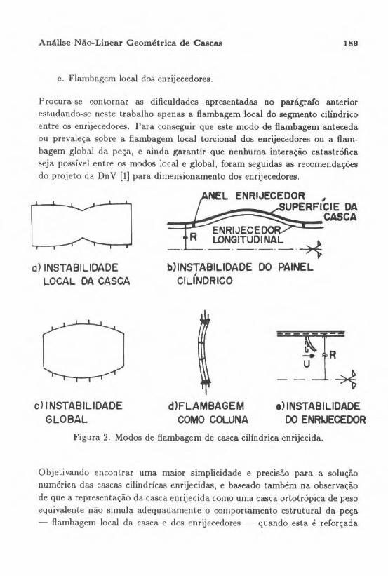
A presença dos enrijecedores longitudinais e/ou circunferenciais, contribuindo para um melhor comportamento estrutural do modelo, fornece entretanto complicações adicionais na estimativa -da carga e do modo de flambagem de uma casca. Em outras palavras, os efeitos específicos que os enrijecedores têm no comportamento de flambagem da casca cilíndrica sob compressão axial são relativamente complexos. Em função das propriedades dos materiais e das características geométricas das cascas e dos enrijecedores, cinco tipos de comportamento de flambagem são geralmente verificados, conforme é mostrado na Figura 2:

a. Flambagem local da casca; b. Instabilidade do painel cilindrico; c. Flambagem global; d. Fla.mbagem como coluna;

Análise Não-Linear Geométrica de Cascas 189

e. Flambagem local dos enrijecedores.

Procura-se contornar as dificuldades apresentadas no parágrafo anterior estudando-se neste trabalho apenas a ftambagem local do segmento cilíndrico entre os eurijecedores. Para conseguir que este modo de ftambagem anteceda ou prevaleça sobre a fiambagem local torcional dos enrijecedores ou a ftam­bagem global da peça, e ainda garantir que nenhuma intera.ção catastrófi ca seja possível entre os modos local e global, foram seguidas as recomendações do projeto da Dn V [1] para dimensionamento dos enrijecedores.

o} INSTABILIDADE LOCAL DA CASCA

c) INSTABILIDADE GLOBAL

d)FLAMSAGEM COMO COLUNA

E -R

~ e) INSTABILIDADE

00 ENRIJECEOOR

Figura 2. Modos de flambagem de casca cilíndrica enrijecida.

Objetivando encontrar uma maior simplicidade e precisão para a solução numérica das cascas cilindricas enrijecidas, e baseado também na observação de que a representação da casca enrijecida como uma casca ortotrópica de peso equivalente não simula adequadamente o comportamento estru tural da peça - flamba.gem local da casca e dos enrijecedores - quando esta é reforçada

190 R .A .M. Silveira e K. Ghavami

por poucos enrijecedores, adotou-se aqui um método de análise que considera a casca e os enrijecedores como componentes estruturais separados, ou seja, um modelo decomposto no qual o elemento de casca enrijecida é discretizado em elemento de casca e de enrijecedor longitudinal (viga-coluna) e/ou enrijecedor circunferencial (anel), como pode ser visto na Figura 3. Métodos similares para o tratamento da interação casca-enrijecedor foram usados com sucesso por Estefen (2}, Andrade [3], Wang e Hsu [4), Ghavami e Andrade [5] e Silveira [6).

ELEMENTO DE CASCA ENRIJECIDA

E L EMENTO DE CASCA

ENRIJECEOOR LONGITUDINAL

(ELEMENTO DE VIGA-COLUNA)

ENRIJECEDOR CIRCUNFERENCIAL

(ELEMENTO DE ANEL)

Figura 3. Elementos de uma casca enrijecida.

DESCRIÇÃO DO MÉTODO DE ANÁLISE

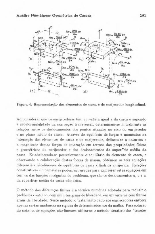
Na formulação adotada, o desenvolvimento das equações de equilíbrio para o elemento de casca enrijecida é baseado na discretização deste elemento em elemeutos de casca e de viga-coluna e/ou anel. Observe através da Figura 4 que o efeito do enrijecedor longitudinal no comportamento da casca é representado pot forças de interação (forças de massa.) que atllam nas direções longitudinal ( FxL), tangencial ( Fn) e radial ( Fz L), e pelo momento de torção interativo (TL), e que localizam-se ao longo da linha definida pela interseção da superfície média da ca.'.lca e o plano médio da viga-coluna. Analogamente são considerada.'> as forças de interação entre a casca cilíndrica e o enrijecedor anelar.

Aláll&e Nio-Linear Geométrica de Cascas

(b)

:).

NAL-t-õNALdx ÕX

(d)

Ul

Figura 4. Representação dos elementos de casca e de enrijecedor longitudinal.

Ao considt-rar qut> os enrijerrdores tém curvatura igual a da casca e supondo

a indefonn<1.bilidade <.la. s11a Se((àO trru1sversal, determinam-se inicialmente as

relações entre os deslocamentos dos pontos situados no eixo do enrijecedor e no plano médio da casca. Através do equilíbrio de forças e momentos na

interseçã.o dos elemeutos de casca e de enrijecedor, definem-se a natureza e

a magnitude destas forças de interaçã.o em Lermos das propriedades físicas

e geométricas do enrijecedor e dos deslocamentos da superfície média da

casta. Estabelecendo-~>e posteriormente o equilíbrio do elemento de casca, e

observando a colaboração destas forças de massa, obtêm-se as três equações

diferenciais não-lineares de equilíbrio de casca cilíndrica. en rijecida. Relações constituti vas e ci nemáticas podem ser usadas para expressar estas equações em

Lermos das funções incógnitas do problema, que são os deslocamentos u, v e w

da superfície média da casca cilíndrica.

O método das diferenças finitas é a técnica numérica ac.lotada para reduzir o

problema contínuo, com infinitos graus de liberdade, em um sistema com finitos

graus de liberdade. Neste método, o tratamento dado aos enrijecedores envolve

apenas certas mudanças na rigidez de determinados nós da malha. Para solução

do sistema de equações não-lineares utiliza-se o método iterativo das "tensões

192 R.A.M. Silveira e K. Ghavami

iniciais", ou mais comument.e conhecido como o método de Newton-Ra.pbson modificado.

CASCA CILÍNDRJCA

É considerado o sistema de eixos coordenados :r , (J e z com origem no ponto P, situado na. superfície média da. casca, conforme representado na Figura 1. Os deslocamentos de um ponto da casca segundo estes eixos são u, v e w, respectivamente.

As relações constitutivas sã.o definidas neste trabalho para os materiais isotrópicos através de um modelo que representa adequadamente as pro­priedades elásticas do corpo. A segu1r, baseadas na teoria geral não-linear de cascas delgadas proposta por Sanders (7]. serão mostradas as relações de­formação-deslocamento e as equações de equilíbrio de forças para o elemento de casca cilíndrica.

Relações Deformação-Deslocamento

AB relações deformação-deslocamento proposta por Sanders, para pequenas de­formações e rotações, e deslocamentos de grandes a moderados, já simplificadas para o caso da casca cilíndrica, sã.o mostradas a seguir:

()u 1 ( 8v tJu):l l ((Jw):l 8w ()ii; !~ = ()x. + 8R2 R tJx - 80 + 2 tJx + tJx ôx

onde, Cz, !o e 1%8 representam as deformações específicas da superíkie média da casca. Nas relações acima já estão incluídos os termos adicionais referentes

Aoállse Não-Linear Geométrica de Cascas 193

às imperfeições geomêtricas iniciais, representadas por w(z, 8) , medidas a partir da superfície média da casca.

Equações de Equilíbrio

As equações diferenciais não-lineares de equillbrio de forças para a casca cilíndrica, já introduzindo a influência dos enrijecedores através das forças interativas, são mostradas abaixo:

8Nr 1 8N:r;8 1 Ô [ ( 8v ôu)] 1 ÔM:&S '"'"'fh" + R ----a8 - 4R2 88 (Nr + Ns) R 8r. - 88 - 2R 802 +

F~L Fxc _O + Ró.O + ó.z -

onde, ó.z e MO representam os espaçamentos, respectivamente, nas direções longitudinal e circunferencial da malha de diferenças finitas a.dotada..

ENRIJECEDOR LONGITUDINAL

Compatibilidade de Deslocamentos entre a Casca e o Enrijecedor

As rela;,.<)..l'> entre os deslocamentos dos pontos situados no eixo do enrijecedor e no plano médio da casca. são definidas conforme a Figura 5, e encontram-se descritas a seguir:

194 R.A.M. Silveira e K. Ghavami

Ü~ = tJ ± eL :X (w + w)

_ ±eL ()( ' ) Ve = v R ()O w + W

ÜJ~ = w + w (3)

Os deslocamentos Üe, ii e e Üle representam os deslocamentos totais de um ponto

qualquer sobre o eixo do enrijecedor; eL é a excentricidade entre o enrijecedor

e a casca. O sinal superior nas expressões acima corresponde aos enrijecedores

fixados internamente na casca, enquanto o inferior pertence aos enrijecedores

externos. A ausência do termo t'/ R, devido a curvatura inicial da casca na direção circunferencial, na segunda equação de (3), pode ser explicada pela

atenção dada neste trabalho apenas às cascas cilíndricas finas . Verifica-se que

em cascas com grandes esbeltez este termo pode ser excluído da análise sem

maiores consequências,

Z(W)

e L

(b)plano 6-Z

(a)plono X - Z

r--4 6ve ~e L ôW ô9

Figura ó. Compatibilidade de deslocamenr.os entre a c as<: a e o enrijecedor .

Análise Não-Linear Geométrica de Cascas 195

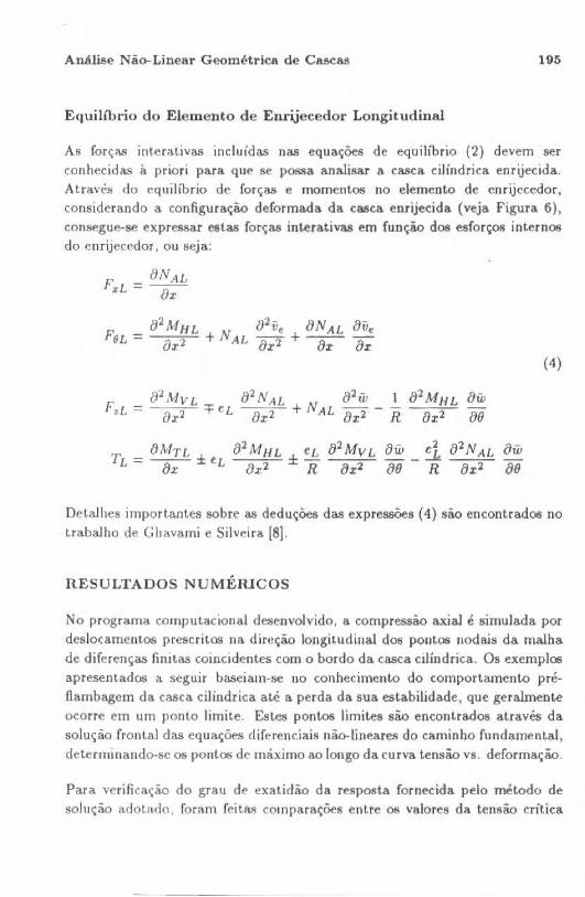
Equilíbrio do Elemento de Enrijecedor Longitudinal

As forças interativas incluídas nas equações de equilíbrio (2) devem ser conhecidas à priori para que se possa analisar a casca cilíndrica enrijecida.

Atravé.., do equilíbrio de forças e momentos no elemento de enrijecedor, considerando a configuração deformada da casca enrijecida (veja Figura 6), co11segue-se expressar est.as forças int.erativas em função dos esforços internos do corijecedor, ou seja:

F.L = 8N,4.L âx

82 M H L fJ2ve ôN AL Ôfíe Fn = ôx2 + NAL ôr2 +a;- ôx

Ô2 \.1 ô2N 82 ô2M ôw-F _ ' VL AL N iv 1 HL bL - âx2 =FeL ôx2 + AL ôx2 - R ôx2 fJO

(4)

Detalhes importantes sobre as deduções das expressões ( 4) são encontrados no trabalho de Ghavami e Silveira [8] .

RESULTADOS NUMÉRlCOS

No programa computacional desenvolvido, a compressão a.xial é simulada por deslocamentos prescritos na direçâo longitudinal dos pontos nodais da malha de diferenças finitas coincidentes com o bordo da casca cilíndrica. Os exemplos apresentados a segu.ir baseiam-se no conhecimento do comportamento pré­flambagem da casca cilíndrica até a perda da sua estabilidade, que geralmente

ocorre em um ponto limi~e. Estes pontos limites são enconLrados através da solução frontal das equações diferenciais não-lineares do caminho fundamenLal, determinando-se os pontos de máximo ao longo da curva tensão vs. deformação.

Para verificação do grau de exatidão da resposta fornecida pelo método de solução ad<>tado , foram feitM compara.ções entre os valores da tensão cn•tica

R.A.M. SUvelra e K. GhavamJ

(b )plano X - Z

(c)plono x-e Figura 6. EquilJbrio do elemento de enrijecedor longitudinal

fornecidos pelo programa cornputaeiona.l para uma. Mca cilíndrica iMtrópir.a. de

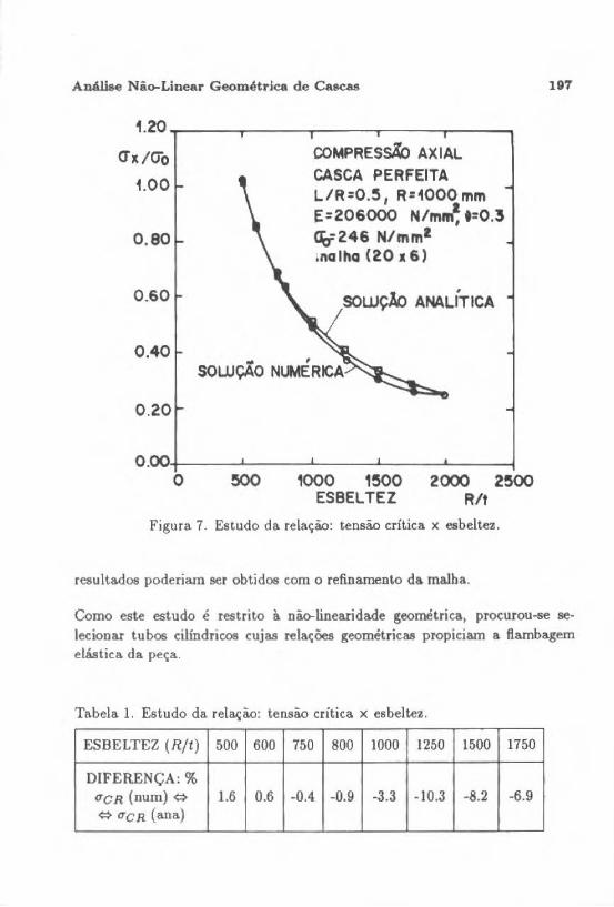
comprimento intermediário e os calculados analiticamente (Vinson [9], Brush e Almroth (10] e Chajes (11]). Os resultados destas comparações podem ser vistos na Figura 7. Verifique a razoável concordância ent:e os valores da tensão crítica obtidos numericamente e os calculados analiticamente para os diversos níveis de esbeltez escolhidos. Baseada nesta figura foi elaborada a Tabela 1, onde são ilustradas as diferenças entre as tensões calculadas pelos dois métodos de anáJ.ise. Ali maiores diferenças observadas para os valores destas tensões correspondem à.s cascas mais esbeltas. Verificou-se entretanto que melhores

Anál.iae Não-Linear Geomêtl'ica de Cascas

1 .20----~--~--~--~---.

O"x / üo

tOO

0 .80

0 .60

0.40

0 .20

COMPRESs.fo AXIAL CASCA PERFEITA L/R=O .~, R=1000 mm E=206000 N/m.J, t=0 .3 ~246 N/mml inalha (20 16)

SOWçlo ANALÍTICA

0 .00•-t-----'-----'---__., __ ___.,____----4

o 1000 1~0 2000 2500 ESBELTEZ R/t

Figura 7. Estudo da relação: tensão c.rítica x esbeltez.

resultados poderiam ser obtidos com o refinamento da malha.

197

Como este estudo é restrito à não-linearidade geométrica, procurou-se se­leciooar tubos cilindricos cujas relações geométricas propiciam a fl.ambagem elástica da peça.

Tabela 1. Estudo da relação: tensão crítica x esbeltez.

ESBELTEZ (Rft) 500 600 750 800 1000 1250 1500 1750

DIFERENÇA:% qCR (num) Ç:> 1.6 0.6 -0.4 -0.9 -3.3 -10.3 -8.2 -6.9 Ç:> qCR (aoa)

198 R.A.M. Silveira e K. G Mvami

Casca C ilíndrica Enrijecida Circunferencialmente

A análise da casca cilíndrica reforçada circunferencialmente é desenvolvida para o modelo estrutural que obedece às relações geométricas R/t = 500 e L/ R = 0.75, onde são considerados dois anéis enrijecedores distribuídos uniformemente ao longo do seu comprimento longitudinaL Os resultados dessa análise para a peça comprimida. axia.lmente são baseados em um diagrama comparativo entre o perfil do desloca.menlo radial total do modelo enrijecido

proposto, no momento em que a carga crítica é atingida, e aquele do painel cilíndrico central entre os enrijecedores idealizado como uma casca isolrópica

com bordos engasta.dos, conforme ilustrado na Figura 8. Note que a deflexão lateral no centro dos dois modelos testados é de mesmo valor. Apesar da semelhança geral no comportamento dos painéis, verifica--se uma diferença marcante entre os deslocamentos radiais nas proximidades do anel.

W/t

_J

< 0 . 80 i5 <( 0::

_J

~ 0 .40 o

L

CASCA ENRIJECIDA (hc= 12mm, tc=4mm)

CASCA PERFEITA

t=2 mm R/t=500, L/R =0.75 E=206000 N/mm~ oQ=0.3 malha (18x8)

CASCA, ISOTROPICA t

'y .... -----' I :\. .

/ 0 .00 '------../---L----.1.-----J.........-::..../ __ ,__ _ _,L.__-J

COMP. LONG. DA CASCA L/2

Figura 8. Casca ci líndrica enrijecida circunferenciaJmente.

A Figura 9 fornece a.s curvas tensão vs. deformação para as duas configurações geométríca.s·proposta.s. Conclui-se que os comportamentos pré-Oambagem são idênticos e que o valor da tensão critica obtida para. o modelo isotrópico idealizado é próximo ao do painel ciliodrico céntral da casca enrijccida.

Análise Não-Linear Geométrica de Cascas

1.20 ,..------r------....------. G"x IO"'o

~0.80 ~

t ct 0.60

'~ ~ 0 .40

~0.20 1-

~NEL ENRI~CIDO

(CENTRAL) ' (!) CASCA ISOTROPICA

o .40 o .80 120 SxiEo

DEFORM. LONG. MEOlAII:EFC9.1. ESCO\M. Figura 9. Análise da relação: l.ensão x deformação.

199

Também verificou-se neste exemplo que o requerimento da inércia radial pro­posto pela Dn V, para dimensionamento do anel enrijecedor, é bastance con­servador e que os resuh.ados obtidos independern da poeição dos enrijecedores (internos ou externos à casca).

Casca Cilíudrica Enrijecida Longitudinalmente

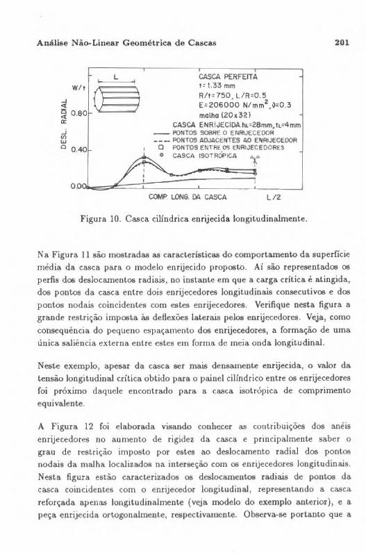
O estudo da casca cilindrica enrijecida longitudinalmente é restrito à con­figuração geométrica com esbeltez Rft = 750 e comprimento longitudinal obe­decendo a relação L/ R = 0.5, onde são considerados oito enrije<:edores longi­tudinais de mesmas dimensões reforçando a estrutura. A Figura 10 mostra, assim como foi feito para o cilindro enrijecido circunferencialmente, um dia­grama comparativo entre os perfis do deslocamento radial da casca enrijecida

200 R.A.M. Silveira e K. Ghavami

e aquele da casca ísotrôpica, no momento em que a tensão critica é atingida. Para representar os deslocamentos do modelo enrijecido, além da consideração de pontos nodais sobre a superfície média da casca coincidentes com os en­rijecedores e pontos nodais locali.zados entre dois enrijecedores longitudinais consecutivos, foram também usados os pontos da casca posicionados nas linhas da malha adjacentes ao en.rijecedor. Excetuando-se o perfil representado por pontos nodais da casca ciündrica coincidentes com os enrijecedores, observe a semelhança de comportamento ent.re os demais. Estes perfis podem ser car­acterizados principalmente por uma saliência externa da superfície média da casca, relativamente acentuada, próxima ao contorno e também pela semelhan­ça dos va.lores das deflexões laterais ao longo de todo o comprimento da casca. A presença desta sa.líência externa relevante po<ie ser explicada pela existência de tensões de fiexão elevadas que surgem em função das restrições impostas pelo bordo da casca.

O ganho de rigidez da. estrutura com a introdução dos enrijecedores longitudi­nais pode ser notado claramente no perfil do deslocamento radia.! dos pontos coincidentes com os eorijecedorcs. Note que para estes pontos, ao longo de todo comprimento longi~udinal da casca, os deslocamentos radiais são menores que os obtidos para os demais pontos da malha.

Neste exemplo foram seguid~ os requerimentoe de projeto da Dn V pa.ra dimen­sionamento do enrijecedçr longitudinal e também aqui os t-estes mostraram-se indiferentes à posição do enrijecedor na parede da casca.

Casca Cilíndrica Enrijecida Longitudinal e Circunferencialmente

Para o caso da casca cilíndrica enrijecida ortogonalmente o modelo estrutural a ser analisado é obtido adicionando-se três anéis enrijecedores uniformemente distribuídos na configuração geométrica do exemplo anterior (casca enrij. long.). As dimensões dos enrijecedores longitudinais e circunfereuciais são tomadas iguais e escolhidas com o propósito de garantir que a flambagem loc.a.l do segmento cilindrico entre os enrijecedores anteceda ou predomine sobre as demais formas de colapsos da peça. As informações encontradas a seguir envolvendo o comportamento da casca ciündrica são, como nos exemplos anteriores, basea.das exclusivamente no estudo do perfil do deslocamento radial total da superfkie média da casca.

Análise Não-Linear Geométrica de Cascas

W/t

;1 ~ 0.80 0::

..J (/) w o 0.40

.--------.----- -r------.------. L CASCA PERFEITA

1= 1.33 mm

R/t=750. LIR=0.5 E=206000 N/mm2,~=0.3 molho (20lt32J

CASCA ENRIJECIDA.hL=28mm, 1L=4mm -- PONTOS SOBRE O ENRIJECEOOR ---PONTOS ADJACENTES AO EIIIRijECEOOA

O PONTOS ENTAt: OS ENRtJE'CEOORES lil CASCA ISOTRÓPICA t"

COMP LONG. M CASCA L 12

Figura 10. Casca cilíndrica enrijecida longitudinalmente.

201

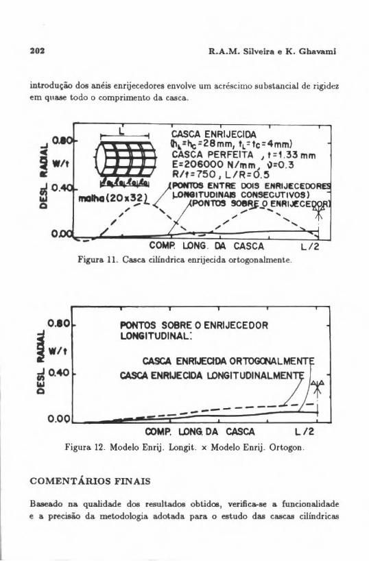
Na Figura 11 são mostradas as características do comportamento da superfície média da casca para o modelo enrijecido proposto. Aí são representados os perfis dos deslocamentos radiais , no instante em que a carga crítica é atingida, dos pontos da casca entre dois enrijecedores longitudinais consecutivos e dos pontos nodais coincidentes com estes enrijecedores. Verifique nesta figura a grande restrição imposta às deflexões laterais pelos eruijecedores. Veja1 como consequência do pequeno espaçamento dos enrijecedores, a formação de uma única saliência externa entre estes em forma de meia onda longitudinal.

Neste exemplo, apesar da casca ser mais densamente eruijecida, o valor da Lensão longitudinal crítica obtido para o painel ciHndrico entre os eorijecedores foi próximo daquele encontrado para a casca isotrópica de comprimento equivalente.

A Figura 12 foi elaborada visando conhecer as contribuições dos anéis

enrijecedores no aumento de rigidez da casca e principalmente saber o grau de restriç.ão imposto por estes a.o deslocamento radial dos pontos nodais da malha localizados na int.erseçào com os enrijecedores longitudinais. Nesta figura estão carac~erizados os deslocamentos radiais de pontos da casca coincidentes com o enrijecedor longitudinal, representando a casca reforçada apenas longit.udinalmente (veja modelo do exemplo anteriorL e a peça enrijecida ortogonalmente, respectivamente. Observa-se porta.n~o que a

202 R.A.M. Silveira e K . Ghavam.i

introdução dos anéis eruijecedores envolve um acréscimo substancial de rigidez em qnase todo o comprimento da casca.

0.10~

,.- L -t CASCA ENRIJECIOA lh.,=hc=28mm, tL =tc=4mm) CASCA PERFEITA J t=1 .33mm E=206000 N/rnm...l \l=0.3 R/t=750, L / R=u.5

/

fiONlt)S ENTRE DOIS ENRIJECEOO rnalha(20x3_21_ }.OMITUOIN~ CONSECliTIVOS)

,; PONT05 90S~ _o !NRI~CE! / / ' ,; .....

/ ,;/ ..... .

COMP. L.ONG . DA CASCA L/ 2 Figura 11. Casca cilíndrica eruijecida ortogonalmente.

J

jwlt PONTOS SOBRE O ENRIJECEOOR LONGITUDINAL:

CASCA ENRIJEQOA OR'TOGCt'<IALMENT~ ~Q40

~~OOA ~TU::~M2_r "' a

L------~~~==:c===-==-=--~::::::::::::~:L_j 0.00 -----COMP. L.ONG DA CASCA L /2

Figura 12. Modelo Enrij. Longit. x Modelo Enrij. Ortogon.

COMENTÁRIOS FINAIS

Baseado na qualidade dos resultados obtidos, verifica-se a funcionalidade e a precisão da metodologia &dotada para o estudo das cascas cilíndricas

Análise Não-Linear Geométrica de Cascas 203

enrijecidas, onde através de uma formulação simples e facilmente automati.zável pode-se conhecer realisticamente o ganho de rigidez da estrutura com a adição doe enrijecedores. Nos exemplos abordados, em função do grande espaA;amento entre os enrijecedores, os valores das defiexões Laterais dos pontos nodais localizados entre dois enrijecedorea consecutivos Dl06traram-ee pró.ximos daqueles observados em uma casca cilíndrica isotr6pica de comprimen~ equivalente.

Convém destacar que, baseado na expenenc1a a.dquirida até o momento, esta forma sistemática de tratamento numérico das cascas cilíndricas com enrijecedores pode ser aplicada às cascas cujas relações geométricas R/te L/ R variam de 500 a 2000 e 0.5 a 1, respectivamente.

Objetiva-se, como etapa subsequente a este trabalho, a inclusão da não­linearidade física do material e uma análise mais rigor06a das tensões predo­minantes que se desenvolvem nos enrijecedores ao longo de todo o procesao de carregamento. Presume-se também que através da mesma formulação teórica &dotada aqui possam ser desenvolvidos bons programas para análise de estruturas laminares.

AGRADECIMENTOS

Os autores agradecem ao Prof. Paulo Batista Gonçalves (PUC-Rio) pelas sugestões e revisão do texto, à lzabel Pereira pela confecção das figuras e ao CN Pq pelo subsídio financeiro.

REFERÊNCIAS

[1] Dn V . Buckling Stren'gth Analysis of Mobile Off-Shore Units, Classification NOtas, October, 1987.

[2] ESTEFEN, S.F. Collapse of Ring Sti:ffened Cylinders. PbD Thesis, Univer­sity of London (Imperial College), 1984.

[3] ANDRADE, V .S. Análise de Cascas Cilíndricas Enrijecidas , Discretizadas em Elementos da Casca e Enrijecedor, por Diferenças Finitas, Tese de. Mestrado, Dep&rtamento de Engenharia Civil, Pontifícia Universidade Católica do Rio de Janeiro, 1985.

204 R.A.M. Silveira e K . Ghavami

[4] WANG , J.T.S. and HSU , T .M. Discrete Analysis of Stiffened Composite Cylindrical Shells. AIAA Journal, vol. 11 , no. 11, pp. 1753- 1761, 1985

[5] GHAVAMJ, K. a.od ANDRADE, V.S . A General Formulation for the Analysis of Stiffened Cylindrical Shells, in Optimization in Mathematical Physics, edited by B. Brosowski and E. Martensen , Verlag Peter Lang, vol. 34, Frankfurt, 1986.

[6] SILVETRA, R.A.M. Análise Não-Linear Geométrica de Cascas Cilíndricas lsotrópicas e Enrijecidas, Tese de Mestrado, Departamento de Engen­haria Civil, Pontifícia Universidade Católica do Rio de Janeiro, 1990.

[7] SANDERS Jr. , J .L. Nonlinear Theories for Thin Shells, J . Appl. Math., vol. 21, pp. 21 -36, 1963.

[8) GHAVAMI, K. e SILVEIRA, R .A.M. Formulação Matemática do Método dos Enrijecedores Discretizados para Casas CilindrÍ<:a$ Reforçadas em Duas Direções, Relatório Interno- R1 10/89, Depart.&mento de Engen­

haria Civil, Pontifícia Universidade Católica do Rio de J aneiro, agosto de 1989.

[9] VlNSON, J .R. Structural Mechanics: Tbe Behavi01· of Plates and Sbells, by John Wiley & Sons , l nc., 1974.

[10) BRUSH, D.O. and ALMROTH , B.O. Buckling of Bars, Plates and Shells, McG raw Hill, 1975.

[11] C HAJ ES, A. S'tabiliLy and Collapse Analysis of Axiaily Çompressed

Cylindrical Sbeils, in SheU S~ructures.: Sr.abi.tity and Su ength , edited by R. Narayana, Elsevier Applied Sciense Publísber.a, London, 198b.

RBCM - J. of u.e Braz.Soc.Mech.Sc. Vot. xrn - ,.v-' - ,.,. tC5-t16 - 1991

ISSN 0100-7386

Impresso no Braaíl

GLOBAL MIXED ADAP TIVE METHODS FOR F INITE ELEMENTS

MÉTODOS ADAPTATIVOS GLOBAIS PARA ELEMENTOS FINITOS

Estevam Barbosa de Las Casas - Membro ABCM Departamento de Enamharia de Estruturas Escola de Engenharia da UFMO Belo Horiu>nte MO, BTuil

ABSTRACT

An adaptive mesh refinement method conjugating on initial remeshing of on u•er­defined grid and a global increo~e in the order of the interpoloting polynomials over the doma.in is de.Jcribed. The error indicotor u.Jed in the implementation o/ the algorithm ii btued on the approzimation of the discretization error b11 the interpolotion error. Emphasu ;, given for lhe implementation of the method for plane problem1 in elasticity.

Keyworcls: Computa.tional Mecba.nics • Finite Element Method • Ada.ptive Proceas • Discretiutioo. Error

RESUMO

Um método ati4pt4tioo para refinamento de ma/Juu é de1crito, conjugando uma redefinição i~cial dD malha determinada pelo wuário com um aumt!Ylto global na ordem do6 políoomio.s de interpolação no domínio. O indicador de erro utilizado na implementtJção do algoritmo é baseado na apro~imaçào do e~rro de discretização peÜ> erro de inJ.e~rpol~ão. O trabolho enfatiza uma implementação do método para probl~1as de elastktdade plana.

Palavras-chave: Mecã.nica Computaciona.l • Método dos Elementos Finitos • Processos Adapta.tiv• • Erro de Discretização

Submetido em Setembro 1990 Aceit.o em Abril 1991

206 E.B. de Las Casas

INTRODUCTION

The development of automatic procedures to improve tbe results obtained from a finite element a.na.lysis ba.s been the subject of much effort since the 70's. The reJeva.nce of the ma.tter can never be overestimated, as an inappropriate discrete model will produce poor results, wbich, even when detected by a criterious analysis of the output, will requi.re the definition of a new model a.nd therefore an increa.se in time and computer effort.

The improvement of an initial mesh requires the minimization of components of the error. A priori error estimates are based on previous knowledge of the behavior of the solution, a.nd although useful for a number of particular cases [1), cannot be used for general problems. Severa! a posteriori error estimators have appeared in the literature [2), and proposed as a bases for adaptive refinement techniques. Convergence of the refinement process is attained when a quasi-optimal, improved mesh is generated, taking the discretization error as

the object function. A trajectory of meshes [3] is generated, ba.sed on the error estimated from intermedia.te results in the adaptive process. The improved meshes in the trajectory provide a better basis for the estimators, accelerating convergence.

The current techniques for the refinements, a.fter estimating the erros, are:

a) To relocate thé nodes in the domain (r method or remeshing)

b) To add new elements in selected parts of the domain (h metbod)

c) To increase the order of the interpolation polynomials in regions where the error is estimated to be large (p metbod).

Strategies b and c bave in common the fact that they increase the number of degrees of freedom in the model, and mixed strategies combining h - p and r -h have been proposed. Ea.ch scheme has its advantages and disadvantages in aspects such as required data structure and management, compa.tibility \'v"Íth existing finite element procedures, complexity of the resulting algorithm, rate of convergence, optimality of the obtained meshes, etc. The choice of an estimator implies in compromises between accuracy and simplicity, the latter involving

Global Mixed Adaptive Methods for Finite Element8 207

computer effort, the former capability to detect critica! regions of the domain, specially for poor initial meshes.

REFINEMENT STRATEGY

Fixing tbe number of degrees of freedom in a discrete model, tbe optimum mesh has a constant discretization error for ali elements [4]. R.emeshing schemes try to obtain an equal distribution of the error by moving the nodes from region.s

witb good estimated accuracy in the results to regions with high error estimates. A measure of error dispetsion is used as a stopping criterion, and tbe obtained mesh is a quasi-optimum model for the defined number of d.o.I.

lf the number of d.o.f. is a.llowed to increase (h and p methods), criticai regions

of the domain must be identified , based on the estimators. Some elements are tben refined, either by subdivision into new elements or by increasing the order of tbe interpolation polynomials. For tbe h metbod, irregular nodes are introduced at ioterelement boundaries, and special data structures and modifications in the assernbly procedure must be performed. Additiona.l

geometric considerations are require<l to avoid regularity problems. For the p

method, neighboriog elements with different interpolation funclions in common sides also generate the need for special data management.

A mixed method , combining the r and the p (or h) method of refinement is described in this pa.per, where a.ll refinements are performed in a global way, involving the entire domain. As the remeshing generates a mesh witb good

bomogeneity of the error, tbere is no need for a search for regions with high

error estímates, and ali elements are candidates for refinement. The ,. - p

met.hod increases in t.his second step the order of ali interpolation polynomials, using a library of bigber order elements. The r - h method [1] proceeds to a global subdivision of every element in tbe model, keeping the characteristics of the original (fa.ther) dements. A program for microcomputers has been

developed in FORTRAN 77 using rectangular elemeoLB for plane problems in elasticity incorporat.ing r - h a.nd r- p refinements.

208 E.B. de Las Casas

ERROR INDICATOR

For the purpose of tbe refinemeot proce.ss, a.n estimation of the local error for the elements is not required, as a.n indica.tion of the ratio a.mong the estima.ted errors in the model is sufficient. This rela.tive measure is called error indicator, providing the basis for compa.rison between the estima.ted accuracy for the elements in the domain .

The interpola.tion enor, measured in tlle Sobolev norm, is used to approx:ima.te the discretiza.tion error in the elements. Tak.ing h2 $ bA, with b a positive constant and A the element area, it can be shown (5J that

where 11 · 11 and I · I are the Sobolev norm a.nd senú-norm, u the exact solution to tbe boundary value problem, k t he order of the interpola.tion polynom.ials, h the diameter of the circle circumscribing tbe element and m a.n integer so tbat O $ m $ k; C a positive constant valid for ali elements in a given mesh and uh

tbe finite element solution .

For the calcula.tion of the norm in the indicator , it is necessary to evaluate derivatives of order k + 1 of the solution u (which in the adaptive process is repla.ced by Uh)· To approxima.te tJk+ 1uhff)xk+1 , a least square fit of l)kuhff)xk

at Gaussian locations is performed, and the resulting function (of order 1) is

used to calculate the required derivatives [llJ.

REMESHING

The first step in the mixed algoritbm consists in modífying the nodal locations to resdistribute the error, ma.king elements with large error smaller a.nd iocreasing the nodal density in regions with large errors. The nodes are attracted towa.rds the center of mass of each element, with a force proportional to the indicated error. The new nodal coordinates are calculated based on the weighted average of the distances from each node to t.he center of gravity of the neigbboring elements, witb the estimated errors as weights. The caJculated change in nodal position is then multiplied by a factor {3, which might. be used to slow down modifications within a retinement cycle. Significant modifications

Global Mlxed Adaptive Metbods for FinHe Elements 209

on a poor discretization may delay convergence of the adaptive process, as the basis for tbe error indicators is not yet accurate.

ln order to maintain the geometry of the boundaries, and to ensure tbat externa.! nodal actions are not relocated during tbe process, restrictions are imposed on the modifications of the mesh. Those restrictions are of two types;

a) The node is not considered in tbe relocation scheme, mainta.ining its original position. This option is specially useful for comer nodes and nodes submitted to externa.! actions (such as point loads)

b) The node is restricted to move within a path fixed in the input data and defined by íts locatíon and that of two other nodes. This option is useful for nodes in the boundary of the domain, and for internal bounda.ries between two different classes of elemeots (such as different material properties). lt should be noted that imposed restrictions constitute restraints to the full optimizatíon of the mesh .

At each nodal relocation, the Ja.cobian of the modified elements is calculated. Wben a Ja.cobian is found to be negative, tbe element is collapsed into a 4 ooded triangle by fix.ing the new nodal location in the tine defined by the neighboring nodes. The nodal forces for distributed loa.ds are recalcula.ted for each rnesh.

GLOBAL REFINEMENTS

After remeshing, assumíng a reasona.ble error distribution in the doma.in, an increase in tbe number of d.o.f. is required to improve the model. hom an original mesh wíth 4 node ísoparametric elements, the program allows ~wo leveis of refinements: the substitution of the elements for 8 or 12 node elements, by the ínsertion of one (or two) nodes per elemenl side at the mid point of each and every element. The parameters related to the new nodes are calculated, induding a redefinition of the nodal loads in case of distributed loading. The refinement within a cyde is done element by element, aod the already generated nodes resulting from a previous element subdivision are skipped, after being identified using an a.rray containing the neighbors to tha.t elemeot. Another consideration to be taken is the increase in the number of Gaussian integration points for bigher order elements. A global h refinement can be performed as

210 E.B. de Las Casaa

an alternative , through the division of every element in the domain into four sub elements.

During global refinements, the attributes for the new nodes are derived from tbe two corner nodes in the side of tbe father element. Boundary conditions and restrictions to relocation are ta.ken as equal to the least restrictive between the two original nodes, and equiva)ent nodal loa.ds are reca.lculated for the refined grid.

SOLUTION PROCEDURE AND ADAPTIVE CONTROL

An over-relaxation solver is used for the systems of linear equations. The system of equations is modified at each refinement cycle, making an efficient solver more relevant. With the use of an interative algorithm, the solutions for previous cycles can be used to accelerate convergence, wbile tbe initial values for the unknowns after a global refinement can be interpolated from the previous result. Tbe number of iteration steps is kept small at each cycle, as only an indication of the erro r is required .

To control the adaptive process, a performance index lP is required, comparing a global measure of the error indicators in two dífferent improvement cycles. As the objective is to obtain an equally distributed error, a measure of the error di.spersion is used as a performance index. ln thi.s work, the selected performance index is given by I P = max e;/ mine i, where e i is tbe error indicator. The process is discontinued when lP reaches an user defined value, or when a limiting number of cycles is performed. Besides these control pe.ra.meters, restrictions to nodal relocations must be provided . The number of Gaussian points for rugber order elements in the p step are modified internaJJy by the program.

APPLICATIONS

Simply supported beam with concentrated load

A simply suported beam subjecLed (E= 2.1 x 107 N fm2, 11 =O, span= 10 m,

widtb= l m) to a. point load (2 x lO" N) at mid-span is used a first applicat.ion of the mi.xed a.da.ptive rnethod, using a.n initial uniform grid consisting of four

Global Mixed Adaptive Methods for Finlte Elements 211

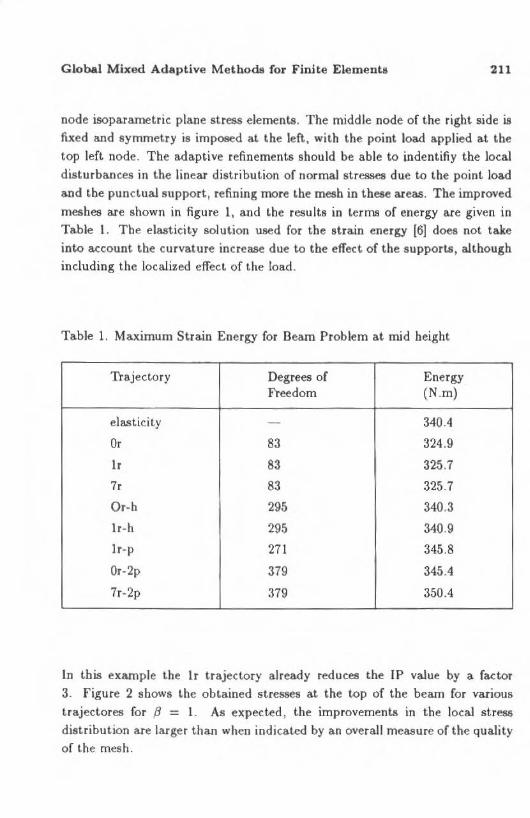
node isoparametric plane stress e.lements. Tbe middle node of the right side is

fixed and symmetry is imposed at tbe left., with the point load applied at the

top left node . Tbe a.da.ptive refinements should be a.ble to indentifiy the loc&l

disturbances in the linear distribution of normal stresses dueto the point load

and tbe punctual support, refining more tbe mesh in these areas. The improved

mesbes are shown in figure l, and the resulta in terms of energy are given in Table 1. Tbe elasticity solution used for tbe strain energy [6] does not take into account tbe curvature increase due to tbe effect of tbe supports, altbough including the localized effect. of t.he load.

Table 1. Maximum Strain Energy for Beam Problem at mid height

Trajectory Degrees of Energy Freedom (N.m)

elasticity - 340.4

Or 83 324.9

lr 83 325.7

7r 83 325.7

O r-h 295 340.3

lr-h 295 340.9

lr-p 271 345.8

Or-2p 379 345.4

7r-2p 379 350.4

ln tbis example the lr trajectory already reduces the lP value by a factor

3. Figure 2 sbows the ob~ained stresses at the top of the beam for various

trajectores for .B = l. As expected, the improvements in tbe local stress dist.ribution are la.rger than when indicated by an overall measure of the qu&lity of the mesh.

212 E.B. de Las Casas

~ 1 --., -

1 ]_ \----\-_j ~- + I 4 ! ~-!---1--1 -~ ~_j_

1-1---+-+-111 rF~~~~ f=+t' ~_J ~t i~ f-l~-,- ~r 1 I I I ~I-'- r - I j

1

- I j I I I I I ' -_L..._ J_ J._ !

FigUie 1. Grids for Beam Problem. Half-span=5 m, Load= 1 x 107N, v= O. Traject.ories: 4r, 7r, Or-h , lr-b.

Global M ixed Adaptive Methods for Finite Elements 213

Stresses (kN/ m**2) 200 ---------------------

100

...........•. .. ----··· .. ·--··- ······-··- ... _._ ... -.......... ....... ~- .

o o

_ _... __ __~_ ____ _ _ j__ -·-----1- -·- - L . - -·- --

0 .2 0 .4 0.6 0.8 1 1.2 1.4

Oistance from axis of simmetry

-~ .. OR -- 1-- 7R - *- 7R-H --{}- 7R-P - - 7R- 2P

Figure 2. Normal stresses at upper boundary for beam problcm.

Membrane sub jected to corner tractions

A membrane of unit thickn ess subjected to traction forces at the corners is analyzed with an initial uniform mesh (figure 3) . T his problem has been previously studied by Carrol [7], who found the optimum mesh for various numbers of degrees of freedom by including the nodal coordinates in the functional to be mínimized by the finite element method. Ta.ble 2 gives the potential energy for different trajec tories takíng f3 = 1, and the resulting gríds are shown in figure 4. Higher gradíents are expected at the corner , with a larger error for the uniform mesh at the regíon dose to the poínt of applications of the load. The restraints to the free relocation of the bounda.ry nodes play an ímporta.nt role ín the optimaJíty of results (1].

314 E.B. de Laa CaaaA

'f bl 2 Dis 1 tsf, t . to . a e p acemen or vanous raJec nes 'Thajectory Degrees of Displacement

Freedom (N.m)

optimum 40 14.4093 Or 40 6.8444 7r 40 8.5986 7r>-p 112 12.8010 7r-2p 184 14.1955 7r-h 144 11.0152 Or-p 112 7.9754 Or-h 144 7.9688 Or-2p 184 8.1544

p

y 100 nm

X

1IIJ nm Figure 3. Membrane problem - P = 25 x 105 N , E= 1 x 107M Pa, 11 = O.

Global Mlxed Adaptive Methods for Finite Elements

í

·\ \ -\- --

1 ____ )-

/ 25x105 N (/ii (

I I

I

'*' Í- -r-r· r

r . -- -

~-

215

J'25xld'N

- I

Figure 4. Grids for membranes. Ttaject.ories: 7r, Or-h , 7r-h .

CONCLUSIONS

The described algorithm provides an alternative path for mesb improvement, performing the bulk of the computational work on a coarse grid , and implementing the refinements in a simple, straigh forwa.rd way. R-p refinements bave shown to be efficient when compa.red to r-h, the latter being more versatile, as it does not require additionai elernents in tbe libra.ry nor modifications in the number of integration points. The problem of high aspect rat.ios can be minimized by an interaction of the user wit.h the program, modifying the initial mesh in arder to avoid constraints in nodal relocation in criticai zones of the domain . A more integrated and efficient equation solver is being developed to t ake advantage of the cha.racteristics of the adaptive process.

216 E.B. de LM Casas

ACKNOWLEDGEMENTS

The aut.hor would üke to acknowledge the financia.] support by CN Pq for t.he development of this work .

REFERENCES

[1) LAS CASAS, E.B. R-h Mesh Irnprovovement Algorithms for the Finite Element Method, Ph.D. thesis, Purdue Universit.y, 1988.

(2] NOOR, A.K. and BABUSKA, L Quality Assessment and Control of Finite Element Solut.ions, Finite Elements in Analysis and Design, 3 ( 1987) 1-27 .

[3] RHEINBOLDT, W.C. Adaptive Mesh Refinement Process for Finite Element Solutions, IJNME, 17 (1981) 649-662.

[4] BABUSKA, I. and RHEINBOLDT, W .C. Analysis of Optimal Finite Element Meshes in 1R.1 , Mathematics of Computation, 33 (1979) 435-463.

[5] DIA'Z, A.R. Opt.imizat.ion of Finite Element Grids Using Interpolat ion Error, Pb .D . Thesis, University of Michigan, 1982.

(6) TIMOSBENKO, S. Theory of Elasticity, McGraw Hill , 1934.

(7] CARROL, W.E. On the Reformulation of tbe Finite Element Method, Compu ter and Structures, 8 ( 1979) 547-552.

RBCM - J . of the Braz.Soc.Mech.Sc. Vot.;'(J/1 - n~ 3 - pp. tt7-t.IO- 1991

ISSN 0100..7386

Impresso no Brasil

A NOTE ON THE VELOCITY OF CRACK PROPAGATION lN TENSILE FRACTURE

UMA NOTA SOBRE A VELOCJDADE IJE PROPAGAÇ.-4:0 DE TRINCAS EM FRATURA A TRAÇAO

Jorge D. Riera CPGEC Universidade Federal do Rio Grande do Sul Porto Alegre - Rio Gr&Dde do Sul Brasil

Mar<:elo M. Rocha Institut für Mec.hanik Universitii.t Innsbrudc Austrla

ABSTRACT

A n overview is given of avoilable Lheoretical $Olutions for the limiting apeed of o propagating crack in a linearly elostic moterial. Within thU context, re.sult.s obtained by means of the dvnomic anoly.sis of a di1crete mcxkl ore given and compartd with the exi.sting prediction equatlons. Finally, a modified equation for tht limiting crack speed, thot ínclude.s the fracture toughnf$S of the material a.s a governing factor, 1s

tentotively proposed.

Keywords: Fracture • Cra.ck Speed • C rack Propagat.ion • Ruptore • Dyna..mic Fracture

RESUMO

Apre8enta.se uma revisão das .soluçõe.s te6rica.s di.spon{ueis para a determinação da velocidade limite de propagação de trincas em materioi.s com comportamento linear eltútiao. Neste contato, .são apresen.tados o.s re.sultados obtidos otrav.é1 da andli.se dinâmica de um modelo dücreto e ccmparadc$ com equações di.sponivei..s no literat'(Jro. Finalmente, propÔe·se umo equação modificada para o cálculo do veloctdode limite de propagação da tl'inca, que inclui o efeito de um fator de tenacidade ô fratura do mete rio/.

Palavras-chave: Fratura • Velocidade de Formação da Trinca • Propagação de Trincas • Rutura. • Fratura. Dinà.mjca.

Subm~Lído ~m Nov~mbro 1990 Ac~ito ~m Junho 1991

218 J.D. Rien and M.M. Rocha

NOTATION a Crack lengtb ao lnitia.l cra.ck length

V Velocity of crack propagation E Young's Modulus

11 Poisson 's coefficient p Specific mass

C'P Velocity of tbe P-wave

CT' Velocity t.he Rayleigh wave K r Stress intensity factor ( Mod~ I)

Krc Criticalstress intensity factor (Mode I)

G 1 Cra.ck surfa.ce energy ft Ultima.te tension stress

t'P Strain a.t ultimate tension stress RJ Rupture factor

k,.n D\)ctility factor for normal bars

A:T'd Ductility factor for diagonal bars D 1 Damping constanL u(t) Applied slress

u(t) Applied displacement

INTRODUCTION

Although unstable crack propa.gation constitues an essentially dynamic phe­

nomenon, the bulk of the work done in fracture mechanics is concerned witb

static solutions aimed at tbe prediction of the onset of sudden rupture. There

is therefore compara,ively little evidence, eitber of theoretica.l or experimental

character, about the dyna.mic cha.ra.cteristics of the rupture process. This is pa.rticularly true in connection with concrete, rock, or simila.rly nonbomoge­neous materiais. ln fa.ct, due to the presence of tbese nonhomogeneities, strong

a.rresting mechanism ma.y hinder the crack propagation, resulting in a sort of

"spasmodic" fra.cturing process .

Precisely n order to study severa.l features of the fracture process in nonho­

mogeneous materia.Js, such as crack velocity, branching a.nd coa.lescence of pre­existings cracks, a. procedure for the determination of the dynamic response of

A Note on the Velocity of Crack Propagatjon 219

a discrete representation of the material is being developed since 1984. The ini­

t ial efforts were düected at tbe reproduction of well established results of linear

elastic fracture mechanics (LEFM), for macroscopically homogeneous materi­ais. Only after verifymg ali aspects of the response and prediction capabilities

of the model, features characterizing different types of nonhomogeneities will

be introduced.

ln this paper, prev1ous theoretical results related to the speed of fracture

propagation in an homogencous material are summarized in a b rief overview,

before the numcrical solutions are deseribed. It is s bown that the numerical

results are fully compa.tible with the available prediction equations for the crack

speed. Finally, on the basis of the entire body of information available to the

authors, a revised equat.ion for the limiting speed of crack propaga.tion in a infinite plate is proposed , which ta.kes into account. the fra.ct.ure toughness of

the material and the applied stresses.

FUNDAMENTAL ASPECTS OF CRACK PROPAGATION

There secms to be sufficient evidence indicating that, under certain ideal

conditions , a. rapidly propagating crack grows with constant speed. Such speed

would then constitute a material property, just. as the P-wave and the 8-wave

velocities in the medium. There have been severa! attempts to determine the

limiting speed of a propagating crack, whích can be classified in two broa.d

groups: theorctical analyses on the basis o f símplified, usually partly static

descriptions and numerical ana.Jyses by means of finite element, finite differences

of discrete models, a.pplied to specific geometrica.l situations bul with less restrictive basic assumptions .

The first thcoretica.I rcsult concerni ng the limiting speed in mode 1 fracture is

generally attributed (Kanninen and Pope lar) fi] to Mott (2] who considered an

infinit.e body subjected to a remote tensile stress q , containing a pmpagating

crack with length 2a(t). Provided that no externa! wo rk is supplied,

conservat.ion of energy then requ ires that

(1)

220 J.D. Riera and M.M. Rocha

in which the first term, contammg an undeterrnined numerical constant 1.:, representa, according to Mott, the kinetie energy associated with a consta.nt cra.ck speed, provided that V < ..fJffTP = c,. The second and third terms

denote the elastic strain energy and tbe work performed in opening the crack, according to the classical Griffith tbeory. If tbe total energy is constant, then its Lotai derivative must be zero

ôL ôL (JV dV + ôa da = O (2)

Assuming now, followíng [2), that dVfda =O, it follows from eqs.(l)-(2) tbat

fhr;aõ V = Cp v k v 1 - -;; (3)

From (3), Mott concluded that the crack speed tends to a limit value that is an (undetermined) fractíon of the P- wave velocity and does not. depend on fracture toughness nor on the stress levei.

Robert and Wells [3] were able to compute the constant 1.: appearing in Mott's

formulation by numerically cvaluating the kinetic energy in quasi static crack growth. Tbus, resorting to West.ergaa.rd's solution for lhe displacements in the static problem, complemented by a judicious choice of tbe limits of integration

- since tbe kinetic energy of tbe plate is not convergent - they ca.lculated , for

a Poisson's value of 0.25, a value J2i7k equal to 0.38. Thus

r;aõ V = 0.38 Cp v l - -;; (4)

Kenninen and Popelar [1], in discussing the pitfalls of Moths' and Roberts & Wells approaches, do point out that experimental va.Jues for Lhe crack speed in botb gla.sses and metais are however in rougb agreement witb eq. ( 4).

Stroh [4) noted tbat if tbe limiting velocíty is assumed independent of the

surface energy, then it should coincide with the Rayleigh velocity. According to this notion , which anticipated later resuJts dueto Freund [5 to 9], the velocity

A Note on the Velocity of Crack Propagation 221

of crack propagation cannot exceed tlle speed CR of a Rayleigh wave 111 the medium. Note that for v = 0.25, CR ===' 0.58 cp.

lndependently, Dulaney and Brace [tO), (see also Aerry (11]), iotroduced a correction to Mott's formulation, eliminating thc nf.'ed for Lhe assumpt.iou lhat dVjda =O. which led to the following limiting crack speed equation

(5)

Of course, lhe problem of evalua.ting k rema.ined open. Adopting Robert.s and Wells [3) value would lead to

. ( ao) V = Ü .• ~8 Cp 1 - -; (6)

Kanninen and Popelar [2] regard any effort t.o improve on eq. (3.6) superOuous, since Freund [5] found that for an infinitc mcdium under tensile loading the limiting crack vclocity is given by

(7)

That. it may not be exactly so will become apparenl in the discus.;ion of numerical result.s. At this point , it is only germane to quote again Kanninen and Popelar , who state that the fact that observed crack specds tend lo agree somewhat. hr.ttcr with eq. (6) than wil.h eq. (7) i:s somewhat for~uitous.

Results from the two dimensiona] elastodynamic problem of a. cra.ck-tip moving wi~h instantaneous speed V in the d irection of the crack path tangent, due to Freund and Clifton (see also Freund [9)), will be reproduced next. These are referred to as crack-tip Cartesian coordinatc systcm (xJ, l:2) with the xz­tlirect.ion coinciding wit.h the crack path tangent direction. The crack sufa.ces are traction free. The spatial dis tribution of s tress and deformation for points in the immedia.te neighbourhood of the cra.ck-tip were determined as an interior asympt.otic expansion, wit.h its dominant term satisfying a standard boundary v alue problem. U nder those limit.ing condit.ions, the following general result

222 J .D. Riera aud M.M. Rocha

was established: for elasto-dynamic crack growth, the spatial dependence of the crack-tip stress components Sij is universal and is given with respect to the local system (x1, :t2) by

s11 = I<J(t) B[(l + 2o-~- a;)cos(8p/2)/(211'rp)t

- 4a 8 ap cos(83 /2)/(1 + a;)(21f r,)t] (8)

s22 = f{l(l) B[- (1 + a;)cos(8p/2)/(21frp)~

- 4a5 ap cos(Os/2)/(1 + a;)(211'rs)~] (10)

as r- O for mode T. The subscripts p and s refer to t.he dila.ta.tional and shear deformations with chara.cteristic wave speeds Cp and c5 • respectively, and

B = (1 +a;)/ R( v)

0 8 = (1 - v 2 /c~)!

R( v)= 4a3 ap- (I+ a;)2

XJ + iasX2 = rseiO,,

( ll)

( 12)

(13)

The stress components haven been normalized with respect to the relation

(14)

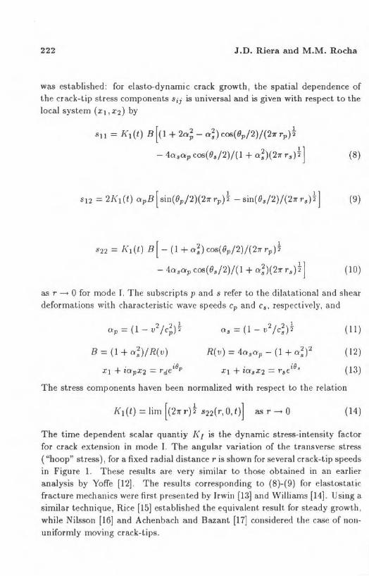
The time dependent scalar quantiy [{ I is t he dynamic stress-intensity factor for crack extension in mode I. 'fhe angular variation of the transverse stress ( "hoop" stress), for a fixed radial distance r is shown for severa! crack-tip speeds in Figure 1. These results are very similar to those obta.ined in au earlier analysis by Yoffe {12). The results corresponding to (8)-(9) for elastostatic fracture mechanics were first presen.ted by Jrwin {13) and Wilbams [14]. Usiug a similar technique, Rice (15) esta.blished the equivalent result for steady growth, while Nilsson [16] and Achenbach and Bazant [17] considered the case of non­uniformly moving crack-tips.

A Note on tbe Velocity of Crack Propagatioo

........ o r-." ........

N N

Vl '-.... ........ ll)

,..: .......... ... ... Vl

1.!>

1.0

0.5

0.0

-0.5

.. ···' ..... ,. .. -·····''

.... ·· ........... .,.._.-.............. .

Values o ( v/c8 :

0.0 0.4 ........ .

0.6 -. - .- .

0.7 ---.

0.8 ··· ··· ···· ···· ··

223

o 20 40 60 80 100 120 140 160 180 Angle 8 - Degrees

Figure I. Angular variation of the hoop stress for the e iMLic near-tip stress field given in ( 8-1 O) for severfi.J crack-tip ~>peeds ( reproduced from Freund f9]) .

DESCRIPTION OF NUMERICAL SOLUTION

The discret.t- model employed in t.ht> studies reported herein starts fro111

earlier development.s in aerona.utical engineering in which , for purposes of

structural analysis it is often necessary to substitute truss.-like structrnal systems by a continuous mediUln. Nayfeh and Hefzi (18] establisbed the equivalence requiriments between the cubic arrangement shown in Figure 2

and on orthotropic elastíc medium. ll ayashi [19] and Riera (20J extensively

tesled tbe model in linear and geornetrically nonlinear analyses of ela . .c~ti c beams.

beam-columns and pla.tes. ln case of an isotropic elastic material , the stiffness

of lhe longitudinal bars in the equivaleni discrete model is given by

(bar length:L) ( 15)

J.D. ruera and M.M. Rocha

while for Lhe diagonal bars

in which

v being Poisson ·s r ati o.

(bar length;VJ L/2)

o=. (9 + 86)/(18 + 246)

é= 9v(4- 8v)

(16)

(17)

(18)

ln the disc rete dynamic model, masses are concentrated at nodal points. The

central finite diRerence scheme is used for explicit numerical integration in the

time domain . Although lhe n•odel proposed by Nayfeh a.nd Hefzi a.dequately

represents the int.erior of an elastic, orthotropic medium, a number of problems

must be soved in the implemeotation of the procedure, oo a.ccount of boundary

e ffecls, since boundary surfaces rare ly interesect only nodal points. ln fact ,

when bars are cut, additional nodes must. be created in the bounda.ry region.

These problems, bowever , are not related with the crux of the matt.er a.nd will

not be further discussed in he re.

The extension of tlle model to Lhe study, initially, of linearly elastic fracture

mec hanics (LEFM) problcms is based on the requirement that, as fracture takes

place. ihe dissipated energy is proportional to tbe newly generated surfaces.

Thus, the so-called llillerborg model shown in Figure 3 is adopted as an effective

stress-strain curve for each individual element.

Let's recall now tbat t.he cri ticai strcss intensity factor in mode 1 fracture may

be expressed in t.be form

(19)

in which ft denotes tbe remote fie ld tensile stress , ao is the fracture s ize and X a nondimensional factor that depends on the problem geometry. On t be otber

hand, the crit ica! s urf;,.ce euergy G 1 is related to/{ /C by mea.ns of

G f = f,·Jc f E'

E'= E/( 1 - v2 ) ( plain strain condition ) (20)

A Note on the Veloclty of Craclc Propagation 225

(o)

z X'

X y

(c)

X

Figure 2. (a) Rasic cubic module. (b) generation of a prismat.ic body and (c)

representation of a plale in plane strai n state (no z-displacemt'nL).

226 J .D. Riera and M.M. !tocha

{o) F ( b) F

Figure 3. (a) Constitutive relation and parameters definition , (b) loading and unloading paths.

Now, since the stress and strain when the loa.d in t be element reaches it.s peak are in the one-dimensional case rela.ted by

!t =E é.p (21)

it may be easily verified that

(22)

in which RJ denotes a rupture factor, defined by Rocha [21J, which can be interpreted as a para.meter quantifying the influence of a real or firtícíou:; material imperfection, ca.us ing Lhe rupture

(23)

As indicated above, the coefficient kr is chosen ín order to sat isfy the requirement that the area under the diagram be proportional to the infiuence surfa.ce for the element under consíderation . For the longitudina.J bars

(24)

A Note on the Velocity of Crack Propagation 227

Substituting in (24) the value of the integral , as weU as the influence area

A 1 = c A L2 , the nondimensionaJ coefficient c A numericaUy evaluated for the

cubic truss model bcing 0.1385. lea.ds to:

(25)

It may be sbown tbat for the diagonal ba.rs

(26)

Note that the a.ppa.rent. ductility coeffcieuts kT giVen ahove depend botb on

material properties a.nd on the geometrical dimensioo L of the elements.

Because tbe energy dissipation in opening the fracture can not be less tban the

strain energy available in tbe element, kr'l , krd ~ L This implies tbat there

is an upper limit for the element length L , which cannot exceed a criticai,

ma.ximum sire. The stress-strain diagram of Figure 3 is hercin designated

elementary constitutive relation ( ecr ). lt was verified by [21] that, for briltle

materiais, Lhe actual shape of the stress-softening branch is a secondary factor

in the cha.racteriz.at.ion of the fracture process. The ecr must not be confused

with macrocoscopic, global, of appa.rent stres.~strain relat ions observed in

testing laboratory specimens. lt must be interpreted as simply a numerical

teclmique t..o assure the c.orrect energy dissipalion.

The model described above was vaJidated by the determination of thc dynamic

response of a rectangular plate in plane strai.n wi~h an initial symmelrical crack,

as shown in Figure 4. The following data applies to Example A:

- Young's modulus : E::: 3.0 x 1010Njm2

- Poison 's coefficient: v= 0.2; (o= 5/ 12)

- Specific mass: p::: 2400kg/m3

- Oamping constant: D f = 2000s- 1 (mass-proportiona.l viscous damping.

resulting for this pla.te in approximatcly2% of criticai)

228 J.D. Riera and M.M. Rocha

·~ I'\/ I'\/ I'\/ I'\/ "\/ "\/ "\./ r'\./ '\../ "\./ r'\./ I'\ I ,.., v !"'V "\V "\V i"\/ 1\. /I'\ /"\ V"\. / r'\. /"\ /'\.V V I'\ 1'\. I'\ V '\V "\V '\/ r'\. V "\.V "\/ I'\ r'\. I

rl/ 1"\l/ "\ l/ v .'\,/ 1"\. [\. / "\V "\. / [\. / "\ V"\ L'\ V I'\ .11"\ / [\. v v V'\. I'\. V v 1'\.

.... l/ I"\ V ""\V ""\ V "\./ I'\ / r'\. /"\ V'\./ v v V "\ V I"\ / I"\ /I""\ /"\ v "\V "\./ r'\. V "\V '\ ./ ~I' r\,/

... v v V"\ V i""\ /'\. I'\/ "\V "\. 1'\. v-

h 1'\ v v "\V "\./'[\. :'\V '\. r--/ r\. V

..... / "\V V'\ V I\ 1'\ 1\.J '\. 1\.. v a-1"\. /I'. / [ ..... / I"\ V '\ v '\V "\.I' r'\. V "\V /"\/ :.;

.... v v 1/ V'\ .l i'- / [\, ~'' V '\. I'\. V .I v

{ t)

1'\ l/ "\ l/r'\. /I\ ./"-., / V'\ .li'\ v '\ V "\ V "\.I r'\. I o ./ ""\.I I"\ V "\ l/ "\/ I'\ v 1'\. 1'\. 1\.. v r I\ / V"\. / "\ /""\ v "\11 ""\/ "\V V"\ v ...... v r-.. I u l/ V '\ 11"- I''\, l'l'. 1'"\ ll f'll/ 1'\. ~ v- { t) I'\/ l/1 '1. / v 'lo, lt"' '\ V l"\11' 'lo, V V'\ 11' r\. I

a v "\.I r'\. V "\ ' ' 1'1.. 1'\ I\.. V I'\ /I\ V I\.: /I' /"\ v v v VI\.. 1/ '\. 11' l'.. V 'li '\t: i'l.. /[\, I/["\ t\.. 1\. /I\ V I\ /r\ / ....... / '\V 1\11' "\V "\ 11 t v 1'\. ' '\ 1'1.. 1'\ 1'\. 1'1.. 1\. I'\ V I'\ V 1\/ v "\11 "\V r\V"\ v

'V i'l.. '\. "\./ '\. ..... V "'.. '\. X

h

Figu re 4. Disn!"tl' representation of the LEFM problem (Example A) considered for validation o f tlae 11umerical model (due to the s iuunetry, jus t

one half o f Lhe single-edge cracked plat.c is modcled) .

Both a unifo rm boundary stres.s u(l) . a ud a uniforru lwunJary displact>tllent

u(t) were applieJ. accorJing to thf' fo llowing laws

(27)

(28)

in which ü. f /h anJ it 1 Jenole Lhe slrain and stress raiRs in l he numericaJ

experiments . Unlt-Ss ol laerwist> ind icaiPd. á1 = l 06(.Njm2 )s- 1, and ÚJ = (O. I h )s- 1. ln s ue h man ncr , t.he expected conditions in a laboratory experiment

A Note on the Velocity of Crack Propagation 229

uoder constant straio (stress) were simulated. Additional deta.ils of these studies are given by Riera and Rocha (20], who discuss the model's ability to predict the velocit.y of crack propagation. Some results, however, will be

reproduced in the following.

For an infinitely long plate, with width h and a lateral crack of length ao,

subjected to remo te tensiJe stress <r, the stress intensity factor is given by

},·, = <ra~ ( 1.99- 0.4l{ao/h) + 18.70(aofh )2

- 38.48(ao/h)3 + 53.85(ao/h)4] (29)

As general indication of the rerformance of the discrete model , the influence

of the a/ h r a tio on the critica] stress is shown in Figure 5 in which lhe values corresponding to stress-coutrolled loading are compared with the static LEFM

expression (29) .

2

t' I (MPo)

I

\ \

o\

' ' ' ' ~ ....

• controUed displacement

o slress-controlled resr

0.1 02

' ... ..... ~

...... ......... ~

...... ...... '-4. -

0.3 0.4 0.5

o/h

Figure 5. lnfluence of tbe a/h ratio on the criticalstress ft for ExampJe A (the curves represent the theoretical solution).

230 J.D. Riera and M.M. Rocha

Finally, the sca.le effect pred1cted by LEFM can be seen in Figure 6, both for displacement or stress-controll~d conditions. The numerical results and the theorelil'fl.l, static LEFM solu tion are virtually identica.l in ali cases, thus providing evidence about the a.dequacy of Lhe model for l he study of fracture in homogeneous media.

f' I

(MPo)

2 • controlled displacement

o stress-cootrolled test

I

- -P __ -o... - ---o- ---A--

0.04 0.10 0.1 4

h(m)

O.lll

Figure 6. Inftuence of Lhe specimen size on the criticai stres.<> ft for Exa.mple A ( the curves represent the theoretical solution).

DYNAMIC CRACK PROPAGATION IN HOMOGENEOUS PLATE

The energy balance in the model during thc numerical integration is carefu lly monitored. Figure 7 f5hows thr> evolution of different forrns of energy of relevance in the ru pture proces.<> in the course of one of the simulation discussed in section 4. The kiuetic energy and the work dissipated by damping werP also computed , but are not included in the graph. Observe that the fract.ure en.ergy

grows smoothly until a pla.tcau is reached, indica.ting the e nd of the rupture process, that is, the complete separation of the plate in two pa.rts.

A Note on the Velocity of Crack Propagation

Energy (Joules)

0.005 -.---------------··-------/ ''\,__/""--._/'·'--"/"--..__/

0.004

0.003

0.002

0.001

o

Total Ener gy ~

-\ \-- Straín Energy

r I \

1,---------------­\ I \ '---1 Fracture Energy

1\ /I.

1 V\l\ A" /\ (\ r=< J - \., \./'·v "

231

O 2.0xiO·S 4.0x i 0·S 6.0x lO·S S.OxlO·S I.Oxl tl ·• 1.2x10·•

Figure 7. Energy componcnts in numerical analysis (Exa.mple A) .

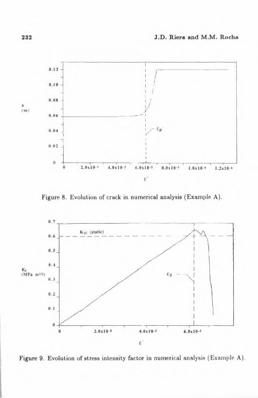
The instanta..neous length of the fracture a(t) is represented, for the sarne case,

in Figure 8. Also note tbat the g lobal deformation €1 associated to the critícaJ

stress occurs somewhat after crack initation. Finally, the evolution of the stress

intensity factor may be seen Figure 9.

The speed of c.rack propagat.ion for vanous values of G f is indicated in

Figure 10. ln every ca.se t.he peak velocity was found to be in the range defined

by eqs . (6) and (7) .

l n fact , appro.xirnate solutious to very similar problems had already been

obtained usiug rtuite element.s by Yagawa et . ai. [22] and finite ditrerences

by Kanazawa et.. ai. [23}, while Broberg [24] had presented earlier a theoretical

solut.ion to the pla.te with a symmetrical notch.

l t should be underliued a.t. t.his point that, as indicated in Section 4, a small

amounL of viscous damping was assumed t.o exist in the model (Kelvin-t.ype

ma.teria.l). Alt.hough t.lw issue is rarely ment.ioned i.n the literature, it is

conc.eivable that. mai.Nial rlamping may also influence thc vclocit.y of crac.k

232

a l mt

0.12

0.1 ()

0.08

0.06

0 .04

~ 0 . 0 2

1 o ()

I I

1/ ,f

-~ '

i ,~

J .O. Riera and M.M . Rocha

!.Oxl0·' -I .OxiO·! 6.0.10· 5 8 .0xiO·S I.OxJO·• l.lxlO·•

Figure 8. Evolution of crack in numerical analysis (Example A).

0.7 ~------------------------

0.6 K1c (statk)

0.5

0.4

0.3

O.l

0. 1

o 2.0>:1 O·S 4.0.10·S

Ep -

-t I I I I I

··~

6.0~ 1 0·!

Figure 9. Evolution of stress íntensity factor in numerícal analysis ( Example A).

A Note on the Velodty of Crack Propagation 233

1000.

800. v, Y ,,,., ;; 672 m/s

(m/s)

600.

400.

200.

o. o 2.0xl0•1 4.0:tlO·S 6.0xl0·1 S.OxJO· S J.OxlO·•

Figure 10. Speed of crack propagation for different values of G 1. The horizontal axis tepresents strain times 105 (Example A).

propagation . ln order to obtain a.d<Üt.ional evidence on lhe influence of both

G 1 and D 1 on the evolution of lhe crack, another plate with different a/ h r ati o

and discretization levei was analyzed.

The geometrical dimensions and the discrete model (Example B) employed are

shown in Table 1 and Figure li. A comparison of the crack velocity with and

without material damping can be seen in Figure 12. Similar results for otber

cases suggest that , for small damping as may be expected in concrete, rock or

metais, viscous material damping may be expected to exert only a secondary

influence on the velocity of cra.ck propagation in mode I fracture. Attention

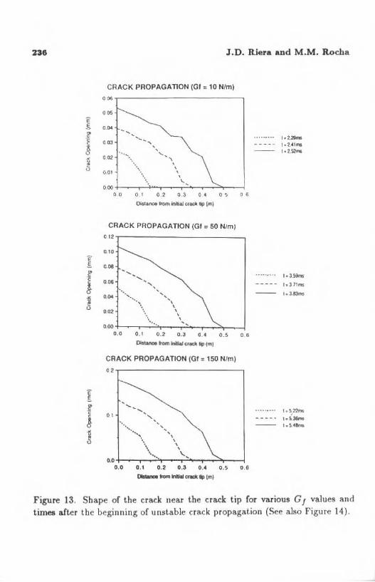
may then be directed to the effect of G 1 and the way of loa.ding. Figure 13

sbows lhe shape of the cra.ck near thc crack t.ip for various C f values and times

after tbe beginning of unstable crack propagation.

234 J.D. Riera and M.M. Rocha

Table 1. Parameters for Example B (Plane strain, stress controUed) E== 3.0 x 1010Njm2 D1 = lOOOs-1 Lc = 0.05m

11 = 0.2 GJ = variable üf = 500MPa '= 2400êgf m3 AI= 8.5ps to= O.OOh

Figure 11. Geometry of plat.e for Example B.

The evolution of the crack speed for the different cases studied (controlled

stresses) is presented in Figure 14. It is a.gain verified that for the most fragile mater ial (Gf = 10 N/m), the peak speed is very close to tbe Rayleigh wave

velocity C.r. As tbe frature toughoess increases, however, the peak velocity appears to t.end to a value somewhat higher than 0.38 c,.

A Note on tbe Veloclty of Craclc Propagation 235

VISCOUS OAMPING INFLUENCE

··· ··- ···· or-o Df'• 1000s-1

o +-----~~~~--~----~~~-----;

2 4 5

Ttme (ms)

Figure 12. Ve locity of crack propagation with a.nd without material damping {Example B).

A CRlTICAL LOOK AT THE VELOCITY OF CRACK PROPAGATION

The results presented i.n last section strongly s uggest tbat t be limiting speed

of crack propagation is inftuenced by the fradure toughness, which does not

appear in eitber Eq.(6) or (7). Jt was verified that, as G 1 tends to zero, the

limit crack speed in the finite plate does approach the Rayleigb wave veJocity.

Moreover , i t decreases with increasing G 1, apparently towards a value around

o r somewhat h igher t han 0.38 C11 • It is interesting to observe that, according to

Figure 1, whe n the cra.ck speed exceeds about 60% of the s hear wave velocity,

then tbe peak hoop stress in the vicinity of tbe crack-tip does not occur at 8 = O, but at 8 ::: 60°, s uggesting a tendency for the crack to follow a curved

path. At a.ny rate, the speed at whicb t he pea.k boop stress no longer t akes

place a.t O= 0° is, rougbly (see also Yoffe [12])

V = 0.60 C8 = 0.60(0.64 C11 ) = 0.38 Cp (30)

236

Ê

J.D. Riera and M.M. Rocha

CRACK PROPAGATION (GI c 10 N/m)

o~

005

s 0.04

I

I !

003

0.02

0.01

\ \ \

\

\.., 0.00 +-~-.--'" ....... ~~,....;:..-...-..,..;:-~-l

0 O O I 0.2 O 3 0 4 O S O 6

0is1anoe lrOm ~ ,._ 1lp (mi

CRACK PROPAGATION (GI c 50 N/m)

012~--------------------------

0.10

0.0 0 . 1 0 .2 0.3 0. 4 0 . 5 0 .6

IA-tam~,._ip(ml

CRACK PROPAGATION (GI = 150 N/m)

02~------------------------~

0.1

·· ....... ' .. ,

\ '\

\ \ ...... '-.. 0.0 -1--.--.-...... .:.:..,.---.....::..--..,...::::---1

0.0 0.1 0. 2 0.3 0.4 0.5 0.6

l:liNra lrOm 1o'ôllal mdt fp (mi

l•l.59ms

lol71ms

lol.&lms

•• ~.22m<

,.s36m$ ..~ ......

Figure 13. Shape of the crack near the crack tip for various G J values and times after the beginning of unstable crack propagation (See also Figure 14).

238 J.D. Rlera and M.M. Rocha

is clearly demonstrated by Lhe spikes prese.nted by lhe V - €1 diagrams of

Figure 12 lt. is admitted t.bat (low) v1scous material damping has a minor

effect oo tbe response. The influence of lhe type aod the velocity of loading

(stress or displacement controlled) are presently uoder investigation.

CONCLUSIONS

As part of the evaluation of a dynamic fracture analysis by means a discrete

model, the numerical solutions for the velocity of crack propagation in an

bomogeneous plate witb an initiaJ lateral crac.k are compared with available

theoretical predictions. lt was verified that the resulta of the numerical analyses

are totally compatible with existing evidence. Jn a.ddition, the model showed

that in finite plates the limiting crack speed tenda to decrea.'>e a.s the fracture toughness increases, conclusion that is possibly applicable as we ll t.o infinite

plates. On that basis, a modified equalion for the limiling crack speed is proposed.

ACKNOWLEDGEMENTS

This research was partly financed by CNPq, FlNEP and CAPES (Brasil). The support of the Bundesministerium für Wissenscbaft and Forschung (Austria)

is also gratefully acknowledged.

REFERENCES

(1] KANNINEN, M.F. and POPELAR, C.H. Advance Fracture Mechanics,

Oxford University Press, Oxford , 1985.

[3] MOTT, N .F. Fracture of Meta.ls : Theoretical Considerations, Engíneeríng,

Vol. 165, 1948, pp. 16-18.

[3] ROBERTS , D.K. and WELLS , A.A. The Velocily of BriUle Fracture,

Engineering, Vol. 178, 1954, pp. 820- 821.

[4) STROH, A.N. A Theory of the Fracture of Metais, Advances in Physics,

Vol. 6, from Phil. Ma.g. Sypol, 1957, pp. 418- 465.

240 J.D. Riera and M.M. Rocha

(18] NAYFEH, A.H. a.nd HEFSY, M.S. Continuwn Modeling of Three­Dimensional Ttuss-Like Spaee Structures, AIAA Journal, 16(8), Aug. 1978, pp. 779-787.

[19] HAYASHI, Y. Sobre um Modelo de Discretização de Estruturas 'fridimen­sionais Aplicado em Dinã.mica não Linear, M.Sc. Dissertation, CPGEC, UFRGS, Porto Alegre, 1982.

[20) RlERA , J .D. Local Effects in lmpa.ct Problems io Conrete Structures. Proceedings, Conf. on Structural Ana.lysis and Design of Nuclear Power Plants, UFRGS, Porte Alegre, Brasil, Oct. 3-5, 1984, Vol. 3, pp. 57-79.

(21] ROCHA, M.M. Ruptura e Efeito de Escala em Materiais N~Homogêneos , Master 's Tbesis, Curso de Pós-Graduação em Engenharia Civil, Univ. Fed. do ruo Grande do Sul, Porto Alegre, Brasil, 1989.

(22] YAGAWA, G., SAK.Al Y. andANDO, Y. Analysis of Rapidly Propagation Crack Using Finite Elements, ín Fast Fracture and Cra.ck Arrest, ASTM STP 627, Ed . by H&hn/Ka.nninen, 1977, 109- 122.

[23) KANAZAWA, T ., MACHIDA, S. and TERAMOTO, T. Preliminary Approaches to Experimental a.nd Numerical Study on Fast Crack Propagation and Crack Arrest, in Fast Fracture and Crack Arrest , ASTM STP 627, Ed. by Hahn/Kanninen, 1977, 39-58.

[24] BROBERG, K.B . On the Speed of a Brittle Cra.ck, Journal of Applied Mechanics, V9l. 31, 1964, 546-547.

RBCM - J. of the Braz.Soc:.Mech.Sc. Voi.Xfll- nl' ~-'PP· !~1-!55- 1991

lSSN 0100..7386

Impresso no B.ra.sil

A NOTE ON THE SOFTENING BEHAVIOR FOR THE BLATZ-KO ELASTIC MATERIAL UNDER PLANE DEFORMATION

UM~ NOTA SOBRE O AMOLECIMENTO DE MATERIAIS ELASTICOS DE BLATZ-KO EM ESTADOS DE DEFORMAÇÕES PLANAS

Edgar Nobuo Mamiya* - Membro ABCM Ad.air Roberto Aguiar Pomi:ficia Unlwnida.de Católica do Rio de Jane.iro 22453, Rio de Janeiro RJ, Brasil

•Present Addreas: butiLuto Politécnico do R.io de Janeiro 28600, Nova Friburgo RJ, Brasil

ABSTRACT

The 11ojtening behauior of the Blatz-K o hyperela11tic material ii analy.sed hcre under homogeneow plane droin conditioru. ll is ob4eroed that thi11 material irutability depend.s not only on the droin 11tale itlelf but al.to on the deformation procu1 COOIIÍdered.

K eywords : Hyperela.slic Materia.Js • Materi&l Softening Beh&vior • M&leri&l lnsta­biMy • Finite Deformations

RESUMO

No pre11ente trabalho, analisa-4c o comportamento dc amolecimento do material hiperelá11tico de Blatz- K o 1ob condiçõCj de dejormoçõe1 plana.t homogénca.t. OblcrtJo· 'e que e11ta írntabílidade material não depM~de 11Ó do e8tado de de/ormoçõc em 11i mClll também do proceiiiiO de deformoçõo con1iderodo.

Palavras-chave: Materiais Híperlá.sticos • Amolecimento • Instabilídcuie Materi&l • Deformações Finita.s

Submetido em Outubro 1990 Aceito em Junho 1991

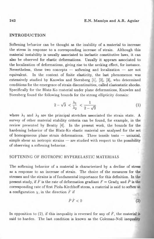
242 E.N. Mamiya and A.R. Aguiar

INTRODUCTION

Softening behavior cao be tbought as tbe inability of a material to iocrease the stress in response to a corresponding increase of strain . Although tbis material instability is usually associated t.o i.nelastic constitutive Laws, it can also be observed for elastic deformations. Usually it appears associated to the localization of deformations, giving rise to the necking effect, for insta.nce. Nevertbeless, these two concepts - softening and localization - are not equivalent. ln tbe context of finite elastícity, tbe last phenomenon was extensively studied by Knowles and Sternberg (1). [2}, (3], who determíned condítions for the emergence of strain discontinuities, called elast.ostatic shocks. Specifically for tbe Blat.z-Ko material under plane deformations, Knowles and Sternberg found the following bounds for the strong ellipticity domain :

rn ~~ 1 2-v~<-<-­

~2 2- v'3 (1)

where ~~ and ~2 are the pr incipal stretches associated the slrain state. A survey of otber material stability criteria can be found, for example, in the review presented by Beatty [4]. ln the present work, the bounds for tbe hardening behavior of the Blatz-Ko elastic. material are analysed for the set of bomogeneous plane strain deformat.ions. Three tensile tests - uniax.ial, simple shea.r an isotropic strains - are studied with respect to the possibility of observing a softening behavior .

SOFTENING OF ISOTROPlC HYPERELASTIC MATERIAL$

The soft.ening bebavior of a material is characterized by a decline of stress as a response to an increase of strain. The cboice of the measures for the stresses and tbe strains is of fundamental importance for this definitioo. ln ~he present study, if É' is the rate of deformation gradiant F = Gradx and P is the corresponding rate of first Piola-Kirchhoff stress, a material is said to soft·en at a configuration x, in the direction F if

(2)

ln opposition to (2), if this inequality is reversed for any of É', tbe ma.terjal is said to harden. The last condition is known as the Colemao-Noll inequality

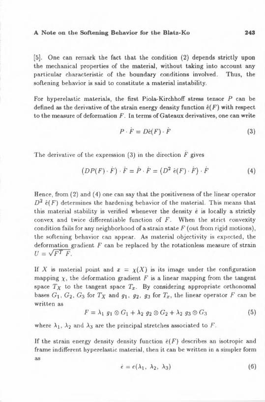
A Note on the Softening Behavior for the Blatz-Ko 243

[5]. One can remark the fact that the condition (2) depends strictly upon the mechanical properties of tbe material, witbout taking into account any particular c.haracteristic of the boundary conditions involved. Thus, tbe softening behavior is said to constitute a material instability.

For hyperelastic materiais, the first Piola-Kirchboff stress tensor P can be

defined as the derivative of the strain energy density function ê(F) with respect to the measure of deformation F . ln terms ofGateau:x deriV&tives, one cao write

p . F = Di:( F) . F (3)

The derivative of the expression (3) in the direction F gives

(DP(F). F). F = p . F = (D2 ê(F). F). F (4)

Bence, from (2) and ( 4) one can say tbaL the positiveness of the linear operator D2 é(F) determines the hardening behavior of the material . This n1eans that this material st.ability is verified wbenever tbe density ê is locally a strictly

convex and twice difTerentiable function of F. When the strict convexity condition fails for any neigbborhood of a strain st.ate F (out from rigid motions),

the softening behavior can appear. As material objectivity is expected, the deformation gradient F ca.n be replaced by the rotationless measure of strain

u = JFT"F.

lf X is material point and x = x(X) is it.s image under Lhe configuration mapping x. tbe deformation gradient F is a linear ma.pping from the tangent space Tx to the tangent space T~. By considering ~ppropriate orthonomal

bases G1, G2, G3 for Tx and 91, 92, 93 for Tz, the linear operator F can be wriLLen as

(5)

where .>.1 , .>.2 and .ÀJ are the principal stretches associa.ted to F.

If the strain energy density density function ê(F) describes an isotropic and frame indifferent hypereLastic material, then it can be writt.en in a si.mpler form as

(6)

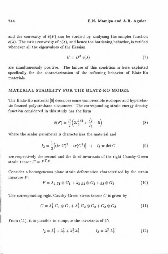
244 E.N. Mamiya aod A.R. Aguiar

and the convex:ity of ê(F) can be studied by analysing the simpler function e(Ã) . The strict convexity of e(Ã). and hence the hardening behavior, is verified whenever alJ the eigenvalues of the Hessian

H= D 2 e(>.) (7)

are simultaneously positive. The failu re of this condition is bere exploited specfic.ally for the characterization of Lhe softening bebavior of Blatz-.Ko materiais.

MATERlAL STABILITY FOR THE BLATZ-KO MODEL

The Blat~-Ko material [6] describes some compressible isotropic and hyperela.s­tic foamed polyurethane elastomers . Tbe corresponding strain energy density function considered in tbis study bas lhe form

ê(F) = ~ (ul/2 + !2 - s) 2 3 13

(8)

wbere tbe sca.lar parameter Ji characterizes tbe material and

h= detC (9)

are respectively the second and tbe third invariants of tbe right Cauchy-Green strain tensor C = pT F.

Consider a homogeneous plane strain deformation cbara.cterized by the strain measure F:

(10)

The corresponding right Cauchy-Green stress tensor C is given by

(11)

From (11), it is possible to compute the invariants of C:

(12)

A Note on the Softening Behavior for the Blatz-Ko 245

Hence, the stra.in energy density function, expressed in terms of the principal

stretches À1 and À2 assumes the repreicntation

(13)

The derivative of (8) with respect to F givee the mechanic.al response function of the Blatz-.Ko material

P(F) = J.l. F. [(detC)1121- c-1). c-1 (14)

or, as a function of the principal strekhes Àt and À2

P(>q, .\2) = 14[(.~2- >.~3) Yt ® G1 + Pt- -'23) 9·2 ® G2

+ (>.1..\2- 1) 93 ® G3 (15)

The material stability considered here is characterized by the positiveness of the operator H = D 2 e(>.). From ( 13)

(3>.-"

H= D2 e(Àt ,>.2) = : (16}

Ea.ch eigenvalue K of H satisfies the condition

det(H - tt 1) =O (1 7)

which can be rewritten, in terms of ( 16) , as:

(18)

The corresponding roots

are both positives provided the term 9>.~" >.;-4 -1 in expression ( 19) is positive. Tbus, the condition

(20)

must be observed.

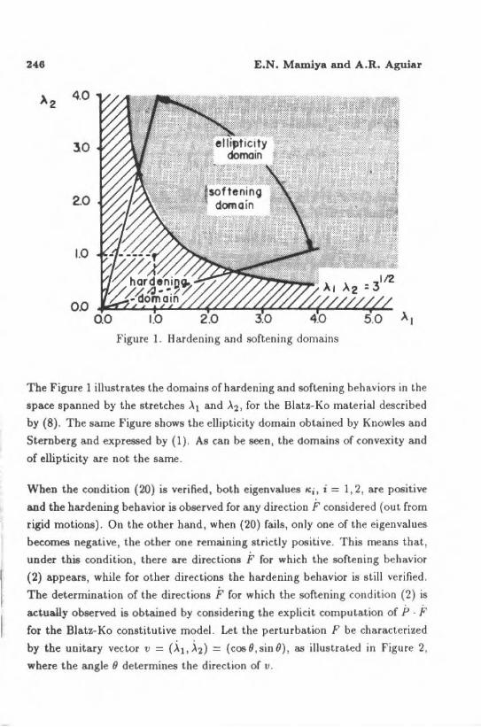
246 E.N. Mamlya and A.R. Aguiar

4.0

30

2.0

1.0

OD

Figure 1. H ardening a.nd softening domains

Tbe Figure 1 inustrates the domai os ofhardening and softening behaviors in the

space spa.nned by the stretches ~ 1 a.nd ~2. for the Blatz-Ko material described

by (8). The sarne Figure sbows tbe eUipticity domain obta.ined by Knowles and

Sternberg a.nd expressed by (1). As can be seen, tbe domains of convexity and

of ellipticity are not tbe sarne.

When tbe condition (20) is verified, both eigenvalues Kj, i= 1,2, are positive

and the ba.rdening beba.vior is observed for any directioo F considered (out from

rigid motions) . On the otber band , when (20) fails, only one of the eigenvalues

becomes negative, tbe other one remaining strictly positive. Tbis means that,

under tbis condition, there a.re directions F for which the softening behavior

(2) a.ppears, while for other directions the hardening beha.vior is still verified .

The determina.tion of the directions F for which the softening condition (2) is

aduaUy observed is obtaioed by considering the explicit computation of P · F for the Blatz-Ko constitutive model. Let the perturbation F be characterized

by the unitary vector v = ( ~ 1, ~2) = (cosO, si o O) , as illustrated in Figure 2,

whe.re the a.ngle 8 determines the direction of v.

A Note on tbe Sof\enlng Behavlor for t be Blatz-Ko

.x2 ~.0

3.0

1.0 ••••••••••• ..,

softenin9

domain

Figure 2. Perturbation of the strain state in the soft.ening domain

The derivative of P(F) in the direction v is given by

wbic.b , specifically for P expressed by (15), gives

P = DP(>.t, >.2) · v

241

=(sinO+ 3>.;4 cosO) 91 ® Gt +(cosO+ 3>.2 4 sinO) 92 ® G2 (22)

+ ( >.1 sinO + À2 cosO) 93 ® G3

A s Ê' is giveo by

F = DF(..\1, À:~) · v= cosO 91 ® Gt +sinO 92 ® G2 (23)

the softening condit ion (2) can be rewritten as

P · F = 3(À-i" 4 cos2 O+ À2 4 sin2 O)+ sin 20 < O (24)

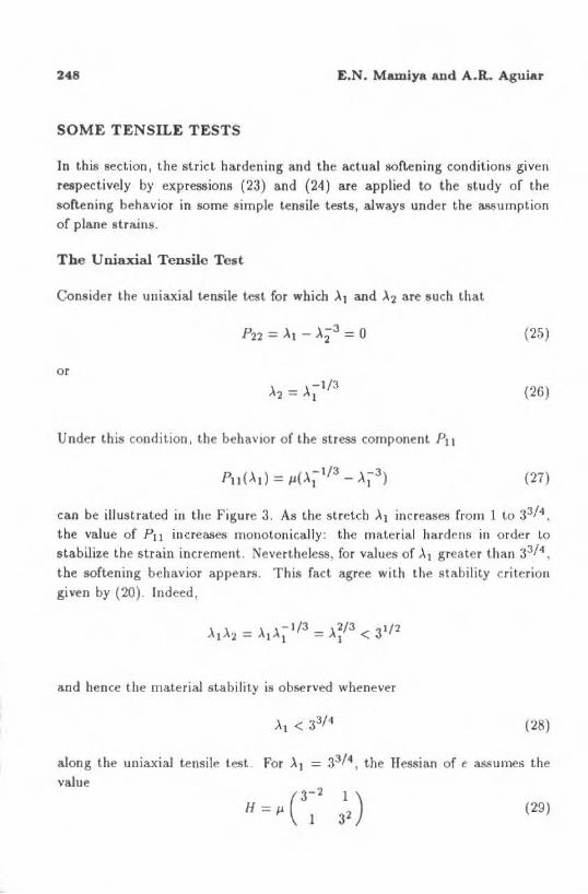
248 E.N. Mamiya and A.R. Aguiar

SOME TENSILE TESTS

ln tb is section, lhe strict hardening and the actual softening conditions given

respectively by expressions (23) and (24) are applied to t he st.udy of the

soft.ening behavior in some simple tensíle tests, always under the assurnptíon

of plane str a.ins.

The Uniaxial Tensile Test

Consider the uniaxial tensíle test fo r which ~ 1 and ~'2 are such that

o r \ - \-1/3 A2- AJ

Under this coodition , the behavior of the stress component P1 1

(25)

(26)

(27)

ca.n be illustrated in the Figure 3. As the stretch ~ 1 increases from 1 to 3314 •

the value of Pu increases monotonically: the materia l hardens in order to stabilize the strain Lncrement. Nevertheless, for values of Ã1 greater than 33/ 4 ,

the softening behavíor appears. This fact agree with the stability críterion

given by (20). Indeed,

and hence tbe material stability is observed whenever

(28)

along the uniaxial tensile t est. For à 1 = 3314 , the Hessian of e assumes the v alue

(29)

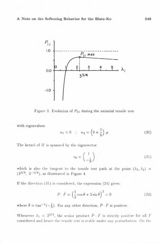
A Note on thc Softeuin.g Bebavior for tbe Blatz-Ko 240

~I 1.0

mt~x

3 4

- 1.0

.f igure 3. Evolution of P11 during the unia.xial tensile test

with eigenvalues

(30)

The kcrnel of 11 ts S IH~ntwcl h} thc· .-igenvector

which is ai!;O t lw laug ... nt lo i.lt t> lens ile test pat.h at the point (..X 1 , À:~ ) = ( 33/ 4 , 3- 1/ 4 ). as tllustrated m Figure 4 .

lf t.he dired.iou (:H) is co nsid t> red, lhe expression (24) giv<'s:

. (I . _) 2 P · F = 3 cos O + 3 sin (J = O

where Õ = tan- 1( -A) For any ot.hl'r direction , p . F is positive.

Whem:ver ..X 1 < :fl/·l , tlw sr alar prod uct P · F is 'l lriclly po~itiv .. for nll 1-' considered anJ lwnc~· th l" l•' tt»il l' I•'S I ts st aldl' under any pnturhation. 011 IIII'

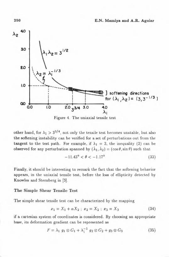
250 E.N. Mamiya and A.R. Aguiar

3.0

1.0

QO 0.0 1.0 2.0 3314 3.0

Figure 4. The uniaxial tensile test

other hand , for A1 > 3314 , not only the tensile test becomes unsta.ble, but also tbe softening inst.ability can be verified for a set of perturbations out from the tangent to the test path. For example, if >'1 = 3, the inequalit.y (2) can be observed for any perturba.tion spanned by (~ 1 ,).2) = (cosB,sin O) such that

(33)

Finally, it sbould be interesting to remark the fact that the softening bchavior appears, in t.he uniaxial tensile test, before the loss of ellipticity detected by Knowles and Sternberg in (3].

The Simple Shear Tensile Test

The simple shear tensile test can be characterized by the mapping

X1 = X1 + oX2 ; X2 = X2 ; XJ = X3 (34)

if a ca.rtesia.n system of coordinates is considered. By choosing a.n appropriate base, its deformation gradient can be represented as

(35)

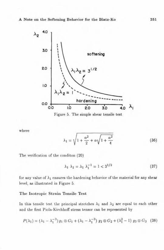
A Note on ibe Softenlng Behllvior for tbe Bllltz-Ko

where

À 4.0 2

3.0

2.0

1.0

I I I

\ \

' \ \

\ \

\ )\,,

softening

À IÀ2 = , ... ......... ......... _ hardening ---·- -----

OD +------r----~--~~~-----0 .0 1.0 2.0 3.0 4.0 À I

Figure õ. The simple shear tensile test

02 g2 l+-+a 1+-

2 4

The verification of lhe conditon (20)

261

(36)

(37)

for any va.Jue of ~ 1 ensures the hardening behavior of the material for any shear

levei, as illustrated in Figure 5.

The Isotl'opic Stt·ain Tensile Test

ln this tens ile lest the principal stretches ~1 and À2 are equal to each other

and the first Piola-Kirchhoff stress tensor can be represented by

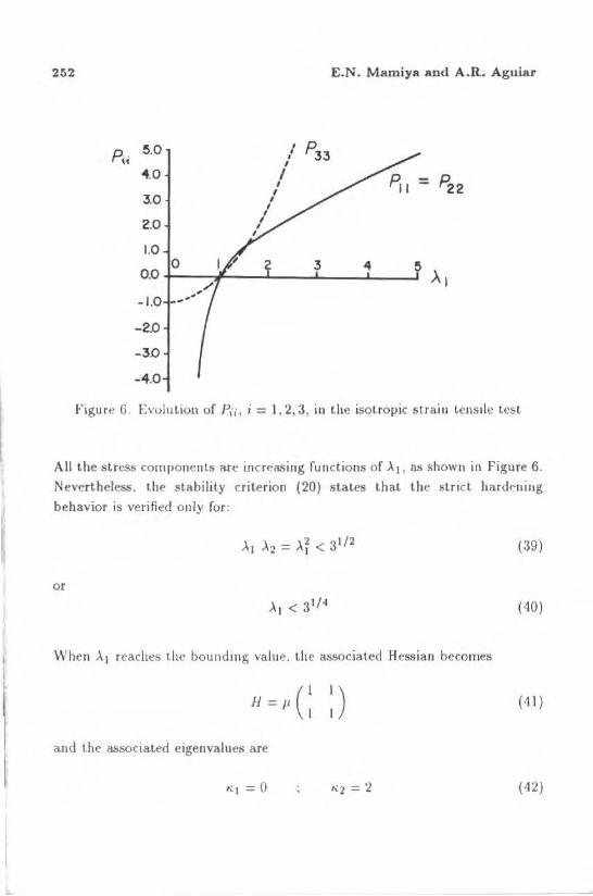
252 E.N. Manúya and A .R. Aguiar

5.0 ,

p33 p.,. , , I

<4.0 I = p22 I

3.0 I I

I

2.0 I I

I

1.0

0.0 o 3

-1.0

- 2.0

-30

-4.0

F igure 6. Evulution of P1·;, i = ), 2, 3, iu t.he isotropic strain tens ile t.est.

Ali the stress componenls are incr~asing functions of ..\ 1 , as shown in Figure 6 .

Nevertbeless. tbe stabilily criter ion (20) states that. lhe strict hardening

behavior is verified only for:

(39)

o r

( 40)

When )q rcaches t.hc bound111g valuc. t he associated Hessia n becomes

( 11)

and thc associated eigenvalues are

h!= o ( 42)

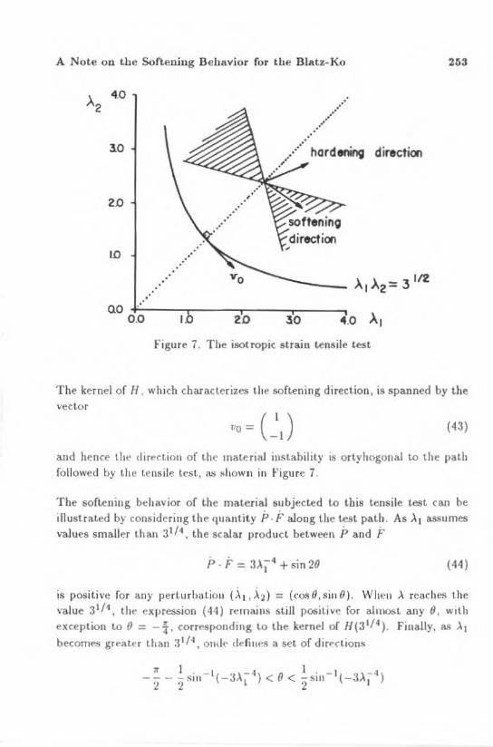
A Note on t.be Soften.ing Behavior for the Blatz-Ko 263

À 4.0 2

3.0 direction

2.0

LO

.· QO

0 .0 3.0

figure 7. Tbe isotrop1c strain ~ensiJe test

The kernel of H , which cbaracterizes th t> softening direction, is spanned by the vector

( 43)

and hence lhe dtrt>rtion of thc rna~enal mstabilily ts ortyhogon al to thc pa~h followed by the tcnsile tcst, ci!S shown in Figure 7.

The soft.eniug bduwior of the material subjected to t.bis tensile test can be illustrated by considering lhe quantity P-É' along the test path . As Àt as,qumes

values smaller tha11 31/ 4 , the se alar produd between P and F

P · F = 3~~4 + sin 20 ( 44 )

is positive for any perturba.tiou (~1 )z) = (cosO,sin 0). When ~ reaches the value 3111 , thf' expression (44) rema.in!t still positive for almost any O, with exception t.o o = -f, corrt'Spondi ng to lhe kernel or H(3 114 ). Finally, as ~, becomes great~r than 3 11", ondf.' defittt•s a se~ of dirf'rtions

1T ) • - 1( .,,- 1) () 1 . -tl 3'-4) -- - - S lll - .JA < < - Slll - A '2 2 l 2 I

264 E.N. Mamiya and A.R. Aguiar

( 45)

'Ir 1 . -1( 3'-4) (} 1 . - )( 3'-4) 2 - 2 SlD - "1 < < 1f + 2 SlD - "1

for whicb the quantity P · F is negative and thus the so{tening bebavior is

verified.

CONCLUDING REMARKS

The softening behavior is studied here specifically for the Blatz-Ko material under the seL of hornogeneous plane deformations. Tbe fact that, even for hyperelastic ma.terials, the softening pehonomenon is not a state property, but

ra.ther presents a. direction dependence, is temarkable . As the global convexity condition is not verified for a.ny objective strain energy density function under the hypothesis of large deforma.tions, the soft.ening behavior should be expected for a. wide class of solid materiais, should the inelastic behavior (and thus the energy dissipation functions) be present or not.

ACKNOWLEDGMENTS

This researcb was supported by FAPERJ under contract number E-29/170.343-88 and by CNPq uoder contract number 305123/88-2.

REFERENCES

[1] KNOWLES , J .K. and STERNBERG, E. On the Ellipticity ofthe Equations of Nonlinear Elastostatics for a Special Material. Journal of Elasticity, 5

(1975) 341-361.

[2J KNOWLES, J .K. and STERNBERG, E. On the Failure of EIJipcity of

lhe Equations for Finite Elastostalic Plane Strain. Archive for JWLional Me<:hanics and Analysis, 63 (1977) 321-336.

[3] KNOWLES , J .K. and STERNBERG , E. On the Failurc of Ellipticity and the Emergence of Discontinuous Defotma.tion Gra.dients in Plane Finite Elastostatics. J ournal of Elasticity, 8 (1978) 329- 379.

[4] BEATTY, M.F. Topics in Finite Elasticity: Hyperelasticity of Rubber, Elastomers, and Biological Tissues - with Examples. Appl. Mech . Rev. 40 (1987) 1699-1734.

A Note on the Sof'tenlng Behavlor for the Blatz..Ko 265

[5] TRUESDELL, C. and NOLL, W. The Non-Linear Field Theoriea of Mecha.nics. Handbucb der Physik , Vol.üi/3, Springer , Berlin.

[6] BLATZ, P.J . and KO, W .L. Application of Finite Elastic Theory to

lhe Deformation of Rubbery Materials. Ttansactiona of the Society of RJleology, VI (1962) 223- 251.

R B CM - J. of the Braz.Soc.Mech.Sc. Voi.XIII - ,..9 3 pp. !!í7- t80- 1991

lSSN 0100.7386 Impresso no Brasil

F ORMULAÇÃ O H A UTO-ADAPTATIVA D E E LEMENTOS DE CONT ORNO PA RA P ROBLEMAS DE ELASTICIDADE

H-ADAPTNE BOUNDARY ELEMENT FORMULATION FOR ELASTICITY PROBLEMS

J.A. Costa Jr.* R.B.V. Pessolan.i** Departamento de EngenhAria Mecãn.ica* Departamento de Engenharia Civit•• Pontiffcia Universidade Cat.61íca do ffio de Janeiro 22453 Rio de Janeiro RJ, Bra.sil

RESUMO

Este arti{JO 11pr-esenta a implementação de um refinamento de malha auto-adaptativo para pmblemas planos de elasl,icidade, usando o .'t-fétodo dos Elementos de Contorno. Uma técnica de redução de er1·o é aJ>Iicado paro controlar a evolução no elemento e na solução global. mediante a comparação da evolução do erro em duas iteraçõu seguidas. Mediante eua técniro, o método decide onde o refiname nto é neceuório. Vório1 ezemplos são alu.slrod~. mostrando a aplicabilidade do m étodo, utilizando /un~es de interpolação constantes, lineo,-cs e quadrdticaJ.

Palavras- chave: Método dos Elementos de Contorno • Refinamento Auto­Adaptativo • Método dos Elementos Finilos •

ABSTRACT

Thia paper pr·esenls U1e tmplemenlation of a self·adaptiue mesh refinement lo solve plane f.la.sticity p•·oblcm-'. '""ing the Bo·tmdary Element Method. An error reduction method "" ulilized wluch ob.serve5 uoriatlon m lhe local elem ent and global Jolutionl for two .sw;cessíue mcshe1. Ba.sed on lheu uolues, the method decide, wMre fv.rther mesh rt:/inement is necded. This adaptive tcchnique i.1 then utilized to analyze variou1 elasticity problems. Num erical result.1 for constant, linCllr and quadratic boundary elcmcnts arr presentcd.

Keywords: Boundary Elemenl Method • Self.Ada.ptive Mesh Refinement • Finite 8lemt'nt Method •

Subme~idn t'm ).1aio 1990 Aceit (• Pm Fe\'ereiro 1991

258 J.A. Costa Jr. e R.B.V. Pessolani

INTRODUÇÃO

Desde o advento dos computadores digitais e acentuando-se at.ualmente a grande difusão dos microcomputadores pessoais, as técnicas numéricas tem sido largamente utilizadas na solução de problemas de engenharia. Com o amemo de um programa de análise de Elementos Finitos ou Elementos de Contorno a tarefa do projetista. passou a ser a de elaborar os dados de entrada, gerando uma malha de elementos e, após a sua execução, a de verificar o grau de precisão dos resultados, baseado na sua sensibilidade e experiência profissional.

Este processo contudo, apesar de ser simples1 pode se tornar demorado, pois

no caso da solução não ser satisfatória, o projetista deve rediscretizar a malha, rearranja.ndo os dados de entrada, e submetendo outra vez o programa. Refaz­se este processo quantas vezes forem necessárias para se alcançar uma solução mais aproximada.

As linhas de pesquisa atuais, estão se voltando para os programas auto­adaptativos, ou seja, programas de aná.lise em que o usuário fornece apenas os dados de geometria e carregamento mínimo para se descrever o problema em questão, e o próprio programa em função de um estimador de erro analisa os resultados e chega à conclusão de quais são as áreas mais afetadas . Toma­se então providências sem qualquer interferência externa segundo as diversas categorias de programas adaptativos:

i) h , que refina a malha em zonas de maior erro;

ii) p , em que o grau da função de interpolação e mudado localmente;

iii) r, o numero de nós é mantido constante e a malha é distorcida de forma a reposicionar os nós em áreas de maior erro;

iv) hp, como uma combinação das duas primeiras.

Este processo, além das vantagens de economia de tempo, possui também a de prevenir contra. possíveis erros de avaliação do projetista, que o leva a considerar como satisfatórios os resultados erróneos.

Formulação H Auto-Adapt.ativa de Elementos de Contorno 259

Em Elementos Finitos a técnica adaptativa tem sido pesquisada por vários autores, entre eles Babuska [05-07], que introduziu estimadores de erro baseados em um desenvolvimento matemático, e Zienkiewickz (21-22] que introduziu um estimador intuitivo, baseado na norma da energia global de deformação e de fácil implementação computacional . Este estimador associado a um gerador de malha, aumenta em muito a eficiência de um programa pelo MEF. Outro trabalho que merece destaque é o de Oden e outros [10], que sistematizaram uma técnica hp para Elementos Finitos.

Em Elementos de Contorno, a técnica P-adaptativa foi inicialmente proposta por Alarcón e outros [2-3), que utilizaram as funções hierarquicas de Peano (ll]. Eles mostraram que a técnica P converge exponencialmente para uma grande variedade de problemas, apresentando contudo alguns inconvenientes nas regiões com singularidade. Esta técnica trás ainda outro inconveniente, que é a de ser necessário o desenvolvimento de programas específicos para este fim, não podendo ser aplicados como um pré e pós processador em um programa de Elementos de Contorno já existente.

Em vista disso, Rencis e MuUen (15-16] desenvolveram a técnica h para problemas de Potencial e Elasticidade, utilizando um estimador de erro baseado na convergência assint.ótica de Wendland [17 -18]. Este estimador feito para elementos com função de interpolação constante, se mostrou bem mais versátil e facilmente aplicável a qualquer programa já existente.

Este trabalho apresenta uma formulação h para problemas de elasticidade baseado nos conceitos proposto R.encis e Mullen nas referências [15-16] . Elementos constantes , lineares e quadráticos são u ~iliza.dos na discretização do contorno e também algumas 1\.ltera<;ões do estimador de erro proposto por Reocis e Mullen [16] foram estudados. Vários exemplos são apresentados de forma demonstrar o aprimoramento da solução do problema com o uso de elementos lineares e quadráticos . Esta formulação tem como grande vantagem a possibilidade de ser implementada. em qualquer programa de MEC, sem ter que alterar a estrutura básica dos programas clássicos de MEC.

260 J.A. Costa Jr. e R.B.V. Pessolani

PRELIMINARES E FORMULAÇÃO DO MEC

A formulação de Elementos de Contorno para problemas de elasticidade bidimensional de corpos elásticos e isotrópicos, baseando-se na identidade de

Somigliana [5]. fornece:

onde pé um ponto do domínio n, q um ponto do contorno r do mesmo domínio, u;;(P, q) e ti;(p, q) são, respectivamente, os campos de deslocamento e forças de superfícies da solução de Kelvin (5] e Cij(P) são os coeficien tes que dependem da geometria do contorno e do ponto p. Os coeficientes C;;(p) são iguais a S;j

se p é um ponto do interior e igual a !éij se p é um ponto do contorno suave,

Óij é o delta de Kronecker.

A solução numérica aproximada do problema é obtida dividindo o contorno em N eelementos, isto é:

(2)

sendo que dentro de cada elemento os campos de deslocamentos e forças de superfícies são aproximados por:

N' n

u;(p) ~ u;(p) == L tPk(q)u7, (q E r n); k=l

N' n

- " k t;(p) ~ t;(p) = ~ 4>.~:(q)t; (q E r n) k=l

(3)

sendo N~ o numero de funções de int-erpolação utilizadas para aproximar a componente i dos campos mencionados anteriormente, no elemento r n.

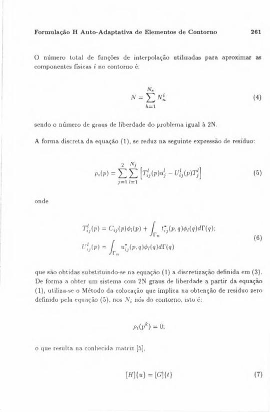
Formulação H Auto-Adaptativa d e Elementos de Contorno 261

O número lotai de funções de inter polação u tilizadas para aproximar as com ponentes fís ica.<> i no contorno é:

(4)

sendo o número de graus de liberdade do problema iguaJ à 2N.

A forma d iscreta da equação (1 ), se reduz na seguinte expressão de resíduo:

onde

'l N;

p,(J1) =L L [r/1 (p)u~- uf,(p)Tj] J=l l=l

Tf1

(71) = C ,j(P)dlt(P) + r t71 (p, q)tPt(q)df (q); ir ..

l ':)( p):. r u:)(p,q).p,(q)dr(q) lr"

(5)

(6)

que são obtidas suhstituindo-se na equação (l) a discretização definida em (3) .

De fo rma a obter um sistema com 2~ graus de liberdade a partir da equação

(1), utiliza.-st' o Método da colocação que implica na obtenção de resíduo zero

definido pela eq uação (5). nos Ni nós do contorno, isto é:

o qut> resu lta na con lwcidn matriz [5],

[H]{u} = [G]{t} (7)

262 J.A. Costa Jr. e R..B.V. P cssolani

onde 1 ::; k ::; N; e 1 ::; i $ 2.

Os coeficientes das matri~es [G] e[H] são obtidos pelas seguintes equações

{8)

(9)

onde as integrais podem ser calculadas usando uma integração numérica tipo Gauss [5].

Uma vez que o problema foi formulado, a equação (1) possui N incógnitas num total de 2N graus de liberdade. Logo, aplicando as condições de contorno, esta

equação pode ser transformada num sistema linear de equações [5]:

AX=B ( lO)

com as seguintes condições de contorno:

U&(q) = u;(q) (q E r u); (11)

ti(q) = t;(q) (q E ft). (12)

onde u;(q) e t;(q) são valores conhecidos no contorno.

FORMULAÇÃO ADAPTATIVA

Atualmente, em métodos numéricos é de considerável importância o controle do erro obtido pela aproximação numérica na solução dos problemas de

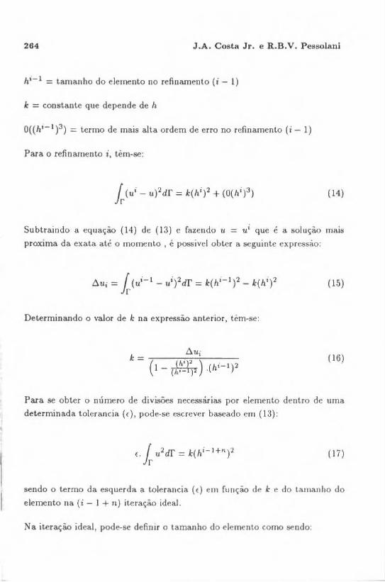
264 J.A. Costa Jr. e R .B .V. Pessolan!

hi-l = tamanho do elemento no refinamento (i - 1)

k = constante que depende de h

O(( hi-l )3) = termo de mais alta ordem de erro no refinamento (i- 1)

Para o refinamento i, têm-se:

(14)

Subtraindo a equação (14) de {13) e fazendo u = ui que é a solução mais

proxima da exata até o momento , é possível obter a seguinte expressão:

(15)

Determinando o valor de k na expressão anterior, têm-se:

(16)

Para se obter o número de divisões necessárias por elemento dentro de uma

determinada tolerancia (f), pode-se esc rever baseado cm (13):

( 1 i)

sendo o termo da esquerda a t{)lerancia (f) em fuuçào de k e do tamanho do

elemento na (i - 1 + n) iteração ideal.

Na iteração ideal, pode-se definir o tamanho do elemento como sendo:

Formulação H Auto-Adapt"tlva de Elementos de Contorno 265

( 18)

onde, n = numero de d1vtSões necessárias para a iteração ideal.

Igualando a. expressão ( 17) em ( 16) e isolando o valor de n, é possível obter a

segui nte expressão:

(19)

sendo;

(20)

onde n1+1 é o número de divisões necessárias para o elemento j na iteração ]

i+ 1.

As equações (20) e ( 17) quando a fun ção u é constanle, fig. 1., reduzem-se às

seguintes expressões·

(21)

(22)

266

. I

u . 1 J-

.. ~

j - t

~

. J

J.A. Costa Jr . e R.B.V. Peuolan.i

u i.- t J

u '· J o n . J

Figura 1 - Elemento constante após duas iterações sucessivas i - 1 e i

As equações anteriores foram deduzidas por Rencis e MuUen na ref. [16). No caso em que é suposta uma variação linear das variáveis do problema, para um elemento j com os nós j e j + 1 pertencentes ao elemento, fig . (2), têm-se:

(23)

Ir N. hi

'2 - "' i [ jl '2 '2 '2] u df- ~ 3· ui+l + ui.ui+l- ui r ;=1

(24)

Para a variação quadrát ica do potencial 110 interior do elemento j, com os nós j 1, j2ej3 pertencentes ao elemento, conforme fig. 3, obtém-se:

. h'· . . . . 1 . A l ) [2( t- 1 ] ) 8( t-1 t ) 2( 1- l ) t..>.tlj = 15 Uj 1 - Ujl + Uj'2 - Uj2 + ttjJ - UjJ +

2( i-1 i ) ( i- 1 i ) ( i-l i )( i- J i ) + ujl - uil . uj3 - ui3 - uj2 - ui2 uj3 - uj3 + 2( t- I i ) ( i- 1 i )] + Ujl - Uj l . tJJ3 - Uj3

(25)

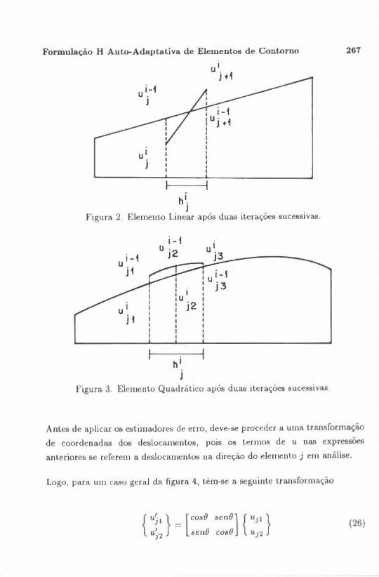
Formulação H Auto-Adaptativa de Elemen tos de Contorno

u' j ••

i-1 u . J

u' j

h'. J

Figura 2. Elemento Linear após duas iterações sucessivas.

u' j i

I I . I I :u : j2 I I I I I

h' J

FigUia. 3. Elemento Quadrático após duas iterações sucessivas .

267

Antes de aplicar os estimadores de erro, deve-se proceder a uma transformação

de coordenadas dos deslocamentos, pois os lermos de u nas expressões

anteriores se referem a deslocamentos na direção do elemento j em análise.

Logo, para. um caso geral da figura 4, têm-se a seguinte transformação

{ uj 1 } _ [cosO senO] { u31 }

uj2

- ser16 cosO u12 (26)

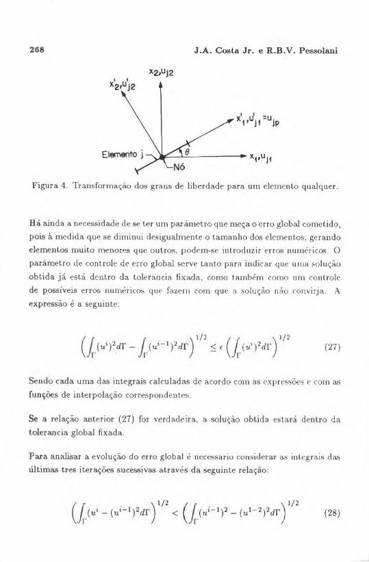
268 J.A. Costa Jr. e R.B.V. Pessolani

Figura 4. Transformação dos graus de liberdade para um demento qualquer.

Bá ainda a necessidade Je se ter um parâmetro que meça o erro global cometido,

pois à medida que se diminui desigualmente o tamanho dos elementos. gerando

elementos muito menores que outros, podem-se introduzir erros numéricos. O

paràmetro de controle de erro global serve tanto para indicar que um(l ::;oluçào

obtida já está dentro da tolerância ·fixada , como t.ambém como um contr ole

de possíveis erros nurnéricos que fazem com que a solução náo ronvirja. A

expressão é a seguinte:

(27)

Sendo cada urna das integrais calcu ladas de acordo com as expressões e com as

funçôes de interpolação correspondentes.

Se a relação anterior (27) for verdadeira., a solução obtida estará dentro da

tolerancia global fixada.

Para analisar a evolução do erro global é necessario considerar as integrais das

últimas tres iterações sucessivas através da seguinte relação:

Formulação H AutG-AdapLaUva de Elementos de Contorno 269

Se a relação anterior for verdadeira a solução estará. convergindo. Caso contrário, estarão ocorrendo erros numéricos que farão com que a soluç.ào não

convirja.. O programa então deverá interromper a sua execução com a resposta mais correta sendo a iter~ão i- I, mesmo que ainda não se Lenha chegado à aproximação desejada.

Foram desenvolvidos os programas ELASTCON, ELASTILIN E ELASTQUA­

para teoria elasticidade com funções de interpolação constant.e,linear e quadrat­ica, e o fluxograma genérico está mostrado na figura 18.

A técnica desenvolvida não prevé a discretização dos elementos com u prescrito. Sendo assim, irnplemeuwu-se uma rotina de discretização destes elementos, em que o usuário fornece o número de divisões desejadas, via teclado. Esta rotina é bastante util, pois apesa.r da solução na maioria dos casos já ser satisfatória, pode-se ainda tentar melhora-la ou obter uma distribuição ma.is uniforme dos

elementos, ou ainda, obter alguns valores intermediarios , sem ter que recorrer a uma inLerpola.ç.ào manual da função.

RESULTADOS NUMtRlCOS

EXEMPLO 1 - Console curto com carga concentrada na extremidade:

Para o caso de elasticidade , resolveu-se o problema clássico de um console curto sujeito a um carregamento uniformemente distribuído na sua extremidade,

conforme mostrado na. fig. 5. O console é quadrado, de lado unitário sendo o carregamento uniformemente distribuído de valor igual a 1,0 N/m. As

constantes físicas do problema est.ào também especificadas ao lado da figura.

O problema foi resolvido pela técnica h-adaptativa. proposta e utiJizando-se as

três funções de interpolação. As discretizações iniciais e finais estão mostradas nas figs . 6 a 8.

Note-se que ocorreu uma discretização não uniforme, ou seja, na extremidade do console onde a variação dos valores dos deslocamenLos é maior , verifica­

se um aumento do número de element.os requeridos para uma boa solução em comparação com as outras regiões do problema. Isto vem constatar a vantagem

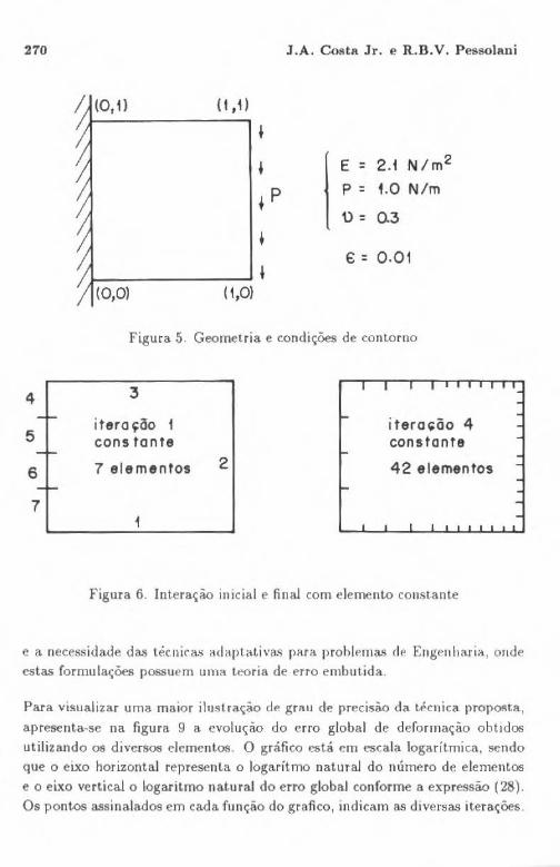
270 J.A. Costa Jr. e R .B.V. Pessolani

(f,1)

+

' I E = 2 .1 N/m2

+ p p = i.O N/ m

'l): 0.3

+ € = 0.01

' ( 1,0)

Figura 5. Geometria e condições de contorno

4 3 -I-

itero~ão i tero•õo 4 5 cons tonte constante -I-

6 7 elementos 2 42 elementos -I-

7

Figura 6. Intera~ão inicial e final com elemento constante

e a necessidade das téc-.nira.o; adaptativas para problemas de Engenharia, onde estas formulações possuem uma teoria de erro embutida.

Para visualizar uma maior ilustração de grnu de precisão da lhnica prop011ta.,

apresenta-se na figura 9 a evolução do erro global de deformação obtidos utilizando os diversos elementos O gráfico está em escala logarítmica, sendo que o eixo horizontal representa o logaritmo natural do número de elementos e o eixo vertical o logaritmo natural do erro global conforme a expressão (28). Os pontos assinalados em cada função do graflco, indicam as diversas iterações.

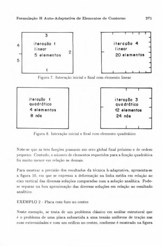
Formulação H Auto-Adaptativa de Elementos de Contorno 2 71

3 I I I I I -i teração iteraçllo 4 -4 I ineor linear -

- 2 ~ -5 elementos 20 elementos -5 . -

1

Figura 7. lnter~ão iniciaJ e final com elemento linear

I I

i teração 1 i tero$ao 3 -quodrótico quodrcHico -4 elementos 12 elementot 8 nós 24 nós -

I I

Figura 8. lnteraçã.o inicial e final com elemento quadrático

Note-se que as t.rés funções po~;suem um erro global final próximo e de ordem pequeno Contudo, o número de <>lementos requeridos para a função quadrática foi muito menor em relação as demais.

Para mostrar a precisão dos resu l~ados da técnica h-adaptativa, apresent.a.-se a figura 10, em que se expressa a deformação na ünha médta em relação ao

eixo verticaJ das diversas soluções comparadas com a solução anaüLica. Pode­se reparar na boa aproximação dM diversas soluções em relação ao resuJtado analítico.

EXEMPLO 2 - Placa. com furo no centro

Neste exemplo, se trata de um problema clássico em análise esLrut.ural que e o problema de uma placa submetida a uma tensão uniforme de Lraçào nas suas extremidades e com um onrício no centro, conforme é mostrado na figun

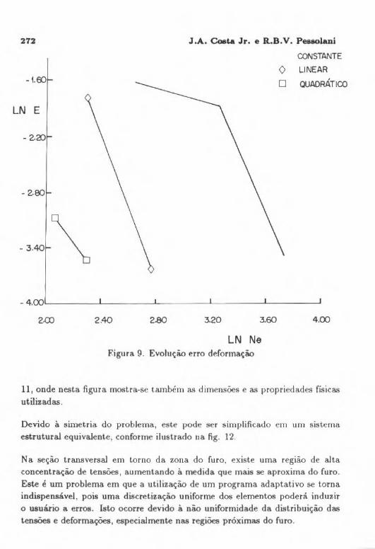
272 J.A. Coe~ Jr. e R...B.V. Pestolani

CONSTANTE

0 LINEAR

- t.€0 QUADRÁTICO

LN E

-2.80

-3~ \

- 4.(X)L-.. ___ _._ ___ ---~.. ____ .L__ _ __ _,_ ___ __..J

2.CO 2.40 2.80 3.60

LN Ne Figura 9. Evolução erro deformação

4.00

11, onde nesta figura mostra-se também as dimensões e as propriedades fiSicas utilizadas.

Devido à simetria. do problema, este pode ser simplificado em um sistema. estrutural equivalente, conforme ilustrado na fig . 12.

Na seção transversal em torno da zona do furo, existe uma região de alta concentração de t.ensões, aumentando à medida que mais se aproxjma do furo . Este é um problema em que a utilização de um programa adaptativo se torna indispensá.veJ, pois uma discretização uniforme dos elementos poderá induzir o usuário a erros. Isto ocorre devido à não uniformidade da distribuição das tensões e deformações, especialmente nas regiões próximas do furo.

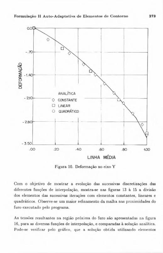
Fol'mulação H Auto-Adaptativa de Elementos de Contorno

(>

o - . 701------1--

ANALÍTICA

- 2.iO,t----- (> CONSTANTE

O UNEAR

O QUADRÁTICO

- 2.80,1------ .._ __ _

273

-3.50~------~---------L--------J---------L--------J .oo .20 .40 .60

LINHA MÉDIA

Figura 10. Deformação no eixo Y

.ao tOO

Com o objetivo de mostrar a evolução das sucessivas discretizações das diferentes funções de interpolação, mostra-se nas figuras 13 à 15 a divisão dos elementos das sucessivas iterações com elemenl.<:xs constantes, lineares e

quadráticos. Observe-se um maior refinamento da malha nas proximidades do furo executado pelo programa.

As tensões resultantes na região próxima do furo são apresentadas na figura 16, para as diversas funções de interpolação, e comparadas à solução analítica. Pode-se verificar pelo gráfico, que a solução obtida utilizando elementoe

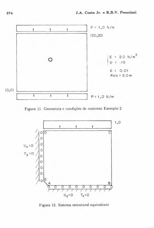
274

lO, O)

o

J.A . Costa Jr. e R.B.V. Pessola ni

P=I,ON/m

(20,20)

I E = 2.0 N/m2

u : .15

€ : 0.01 Raio= 2.0 m

P=I,ON/m

Figura 11. Geometria e condições de contorno Exemplo 2

1,0

I o o c o

Ull=O o o

Ty =O o o o o

E O A 8

1Y1Y1YOO O O O O I I I I I I I I I I I I I I

Uy=O Tx=O

Figura 12. Sistema estrutural equivalente

Formulação H Auto-AdaptativA de Elementos d e Contorno

iteração 1 constante

14 elementos

ít era~ão 3 constante 60 elementos

Figura 13. Iteração inicial e final com elemento constante

itera~ão 1 linear

12 elementos

i tero~ão 5 linear

43 elementos

Figura 14. ltera~ão inicial e final com elemento linear

itera~ao ~ quo drdtico

8 elementos

itera~ão 3 quadrótico

21 elementos

Figwa 15. Iteração inicial e final com elemento quadrático

275

276 J.A. Costa Jr. e R..B.V. Pessolani

quadráticos está em perfeita concordância com a solução analitica para este ponto crítico do problema. A tensão obtida neste ponto foi de 2,99 MPa, muito próxim.'\ ao valor analítico que é de 3,0 MPa. Uma melhor aproximação poderia ser obtida utilizand~se elementos curvos.

o EXATA l<t o CONSTANTE CJ)

z IJJ .......

o UNE AR

o QUADRÁTICO

1.40

j_(X).__ ___ _._ ___ ___..__ ___ _._ _ __ ___.~----'

{.(X) 1.40 i.80 2.20 2.60 3.00

ELEMENTO A-8

Figura 16. Tensões na sessão do furo

No gráfico 17 ê mostrado a evolução do erro global para deslocamentos para cada iteração, em função do número de elementos. Notar-se uma maior precisão com um menor número de nós quando se utilizam elementos quadráticos.

Formulação H Auto-Adaptativa de Elementos de Contorno

.oor-----~r-----~r------.-------.-------,

,-

-I

0 CONSTANTE 0 LINEAR

O QUADRÁTICO

• 7.001L._ ____ ___j~ ____ __J ______ --! ______ __._ ______ __,

2.00 3.60 4 .40 5.20

LN Ne

Figura 17. Evolução erro deformação

CONCLUSÕES

277

Foi apresentado em medidor h adaptativo para o Método dos Elementos de Contorno, apücada a problemas de Teoria da Elasticidade.

Como vantagens da formulação h-adaptativa apresentada pode-se destacar a simplicidade de implementação em programas de MEC, não sendo necessário o desenvolvimento de programas especificas para este fim, podendo ser aplicado como um pré e pós-processador para qualquer programa de análise. Observou­se também que o medidor de erro a.dotado fornece bons resultados, mesmo na presença de zonas de singularidade, onde se exige uma maior discretização pela alta variação de deslocamentos.

A pesar do estimador ser baseado na variação de deslocamentos e de serem refinados sómente os elementos em que o deslocamento é prescrito, mostrou-se

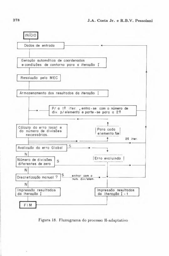
278 J.A. Costa Jr. e R.B.V. Pessolanl

Dados de entrado I I

Geração outomáttco de coordenados e condi(;Ões de contorno poro o iteroç:õo I I Resolução pelo MEC I

Armazenamento dos resultados do iteraç:õo I I

- PI o 12 i ter. , entro- se com o número de di v. p/ elemento e porte- se poro o 2 2

Cólculo do erro loco I e do número de divisões

necessórias . I

............... ! ____ .... ., Poro cada I . elemento Ne:

.. .... ........ f 29 i ter.

Avol ioçõo do erro Global 11--'='-5 - --- ----,~

N f Erro evoluindo ! Número de divisões I S

:'::~::::~:· :::., 7

ls;__ _ _,.""n:.;;,rc.;:o..:.,r ,.:C:::O:;:-m:.,...=..o _._ .. ·• .... -=r --N num. dtv /elem. J

~-~~--~~--, Impressão resultados J llmpressõo resultados I do lteroç:õo I do lteroç:õo I - 1

I F ,' M 11---------------..JJ

Figura. 18. Flu.xugrama do processo H-adaptativo

Formulação H Auto-Adap~tiva de Elementos de Contorno 279

que a precisão obtida para 06 demais elementos é satisfatória. Para se melhorar

a solução nessas regi&>..s obtendo uma discretização mais uniforme, recorreu-se

a uma rotina em que o usuário entra com o número de divisões para cada

elemento. Esta rotina levou a uma maior precisão dos resultadO$.

Como futuros trabalhos, pode-se destacar o desenvolvimento de um medidor de

e rro voltru.lo para a técnica hp e que análisa além da variação dos deslocamentos,

a variação de tensões. O medidor deverá detectar também as áreas onde será

necessário aplicar a técnica h , subdividindo os elementO$ e onde aplicará a

técnica p, aumentando o grau de interpolação dO$ mesmos.

REFERÊNCIAS

[1] Alarcón, E .. Reverter, A. e Molina. J ., Hierarchical Boundary Elements,

Comp. and Struct., 20, 151-156, 1985.

[2] Alarcón, E. c Reverter, A., P-Adaptive Boundary Elements, Int. J . Num.

Meth. Engng, 23, 801-829, 1986.

[3) Alarcóu, E., Avia L. e Reverter A. 1 On the Possibility of Adaptive Bounda.ry

Elements, Proc. of lhe int . Conf. on Accuracy Estimates and Adaptative

R.efinements in Finite Element Comp. (ARFEC), Lisboa, 1984.

(4) Alarcón, E., Cerrolaza, M .. Gong- Lera, M.S., Elastost.atics p-adaptive B.E.

for micros, Software for Engng. Workstation, January, vol. 4, 1988.

[5} Babuska l. and Szabó, On Lhe Rates of Convergence of the Fiuüe Element

Method, lut. J. Num. Meth . Engng, vol 18, 323-341, 1982.

[6] Babuska.l. and Dorr M .R., E r ror estimat.es for tbe Combined h and p Version

of the Finite Element Metho<l , Numer . Math , vol 25,257-277, 1981.

[7] Babuska, 1., and Rheinboldt, W.C., A Posteriori Error Estirnates for Finite

Element Computations, SIAM J . Numer. Anal., vol. 15, 736-754, 1978.

[8] Brebbia, C.A., The B.E.M . for Engineers, Pentech Press, London, Halstead

Press, New York, 1978.

[9] Carey, G.F'. e Kennon , Adaptive Mesh Redistribution for a Boundary

Method, Int .. 1. Num . Met.h. Engng., 24, 2315-2325, 1987.

280 J .A. Costa Jr. e R .B.V. Pessolani

[10] Onden, J .T., Demkowicz L. , Ra.chomicz W . e Hardy 0., Tomard a Universal H-P Ada.ptive Stra.tegy, Comp.Meth. in Appl. Mech . and Engng, vol. 77 , n2 l e 2 , 1989.

(11] Peano, A.G., Riera.rchies ofCoofoming Finite Elements for Plane Ela.sticity

and Plane Bending, Comput. and Maths. with Aplls. 2, No. 3-4, 1979.

(12] Raok, E., Adaptive B.E.M ., Bounda.ry Elemeots IX, C.A. Brebbia Eds . , pag. 259-278, 1984.

[13] Rank , E., A Posteriori Error Estimates a.nd Adaptive refinement for Some

Boundary Integral Element Met.hods, Proc. ofthe Int. Conf. on Accuracy

Refioemeots in Finite Element. Comp. (ARFEC), Lisboa, 1984.

[14) Rank , E., Adaptive h-, p- and h-p Versions for Bounda.ry Intergral Elements

Metbods, Int. Jour. for Num. Metb. in Engng, vol. 28 , 1335-1349, 1989.

[15] Rencis , J .J . e Jong, K.Y., A Self-Adaptive H-Refinement Technique for the

B.E.M., Comp Methods in appl. Mecb. and Eng. , 1988.

[16] Rencis, J .J . e Mullen, R. L ., Solution of Elasticity Problems by a Self Adap­

tive Mesb Refinement Technique for Boundary Element Comput.ation,

Int . J . Num. Meth. Engng., 23, 1509-1527, 1986.

[17] Wendland, W.L . Asymptot.ic Accuracy a.nd Convergence, em Progr('.SS in B.E.M. (C.A. Brebbia Ed .) 289-313, Pent.ech Press, London , Plymouth ,

1981.

[18] Wendland , W.L. , On Asymptotic Error Analysis a.nd Uoderlyning Mathe­ma.t.ical Principies for B.E .M., em Boundary Element Technique in Com­

puter Aided Engineering, (C.A. Brebbia Ed.), Martines Nijhoff Plub­üshera, 417-436, 1984.

[19] Wendland , W., SpHnes Versus Trigonometric Polynomíals, h-versus p­

version in 20 Boundary Intergral Methods, Preprint Nr. 925, TH

Darmstedt, Fashbereicb Mathematik, 1985.

!20] Wendland, W .L. and Yu , D. , Adaptive B.E.M. for Strongly Elliptk Integral

Equations, Semina.r Analysis and Anwendungen, Universitat Stuttgart, Mathema.ttuber lnstitut A., Bericht Nr 4, 1988.

(21] Zienkiewicz , O.C., Gago, J .P. and Kelly D.W., Tbe Hierarchical Concept

in Fnit.e Eement Aalysis, Computers & Structures, vol 16, 53-65,1983.

Formulação H Aut<rAdaptatlva de Elementos de Contorno 281

[22} Zienkiewicz, O .C . and Zhu , J .Z., A Simple Error Estimator and Ada.ptive Procedure for Praticai Engineer ing Analysis, ln I.. J . Num. Mel. h. Engng, vol 24 , 337-357, 1987.

OBJETIVO E ESCOPO

A Revista Brasileira de Cltncias Meta nicas visa a publicaçao de trabalhos voltados ao projeto, pesquisa c desenvolvimento nas grandes áreas das Cltndas Mcc!nicas. É Importante apresentar 06 resultad06 e as conclusões d06 tcabalh06 submetid06 de forma que sejam do interesse de engenheiros, pesqvisadorc:s e docent"-

0 escopo da Revista t amplo e at:range as úeas essenciais das Cltncias Mednicas, Incluindo interfaces com a Engenharia Civil, El6trica, Metalúrgica, Naval, Nuclear, Qufmica e de Sistemas. ApllcacOes da Ffsica e da Matemática â Mecânica também scrao consideradas.

Em geral. 06 Editons incentivam trabalh06 que abranjam o desenvolvimento e a pesquisa de métod<lc tradicionais bem como a introduçto de novas idéias que possam potencialmente ser apt'OYcitadas na pesquisa c na indústria.

AIMS AND SCOPE

The Joumal of the Brazilian Society or MechanicaJ Sciences is concemed primarily with the publication or papers dealing with design, reseaiCh and dcvelopment relating to the general arcas of Mechanical Sciences.lt is important that thc results and the conclusions of thc submined papers be presented in a manou wbich is appreciated by pnctlcing enginecrs, rescaiCben, and educato.rs..

The &eope of tbe Joumal is broad and cncompasses essential arcas of Mechanical Engincering Sciences, with interfaces with Civil, Eletrical, MetaUurgical, Naval, Nuclear, Cbemical and System Engincering as weU as with thc areas of Physics and Applied Mathematics.

ln geneml, thc Editors are looking for papers covering botb development and rescarcb oC traditional methods and lhe introduction of ooYd ideas wbich b.ave potential apptication in sdence and in the manuíacturing indust:ry.

Notes and lnstructions To Contributors

1. Tbe Edito:rs are open 10 receive contributioos from aU parts of the world; manuscripts for publication sbould be sent 10 the Editor-l:n-Cblef or to lhe appropriate Associate Editor.

2. (i) Papers offered for publ.ication musl contain unpublishod material and will be referecd and assessed with refcrencc to thc aims of thc Joumal as statcd above. (il) Rcvicws should constitute an outstandlng criticai app.raisal er published materiais and will be publisbcd by suggestion of lhe Editors. (iii) l..etters and communicatioos to the Editor sbould oot extecd 400 wonls in lcngtb and may be: Criticism of articiCi recently publisbed in lhe Journal; Preliminaty announccmcntli of original work of lmpol'tall« warranting immcdiate publica tio o; Comments oo currcnt engineering matters oí coosiderable actuality.

3. Only papers not previously publisbed will be accepted. Authors must agree not to publisb el$ewbere a pape r submitted to and a.cceptod by tbc JournaL Exteption can be made in some C8ie$ of papcrs publisbcd in annals or proceedings of conferences. The decision on acceptancc of a paper wiU be taken by tbc Edltors considcring tbe revicws of two outstanding &eientists ao<) lts originality, and contribution to science and/or tecltnology.

4. AJJ contributions are to be in E.nglisb or Ponugucse. Spanish wiJJ also be considered.

S. Manuscriptubould begin with the title of thc ankJe, iocluding the eoglish title,and tbe autbor's oamcanda.ddress.ln the case ofco-autors, bothaddressessbould be cleartylndicated.lt follows the abstract; iC the papcr's languagc is different from engtish, an extcodcd sununary in thls language should be included. Up to five >Nords·for the pape r are to be givcn. Next, if possible, sbould come tbe nomenclature list.

6. Manuscripts sbould be typed witb double spacing and wilh amplc rnargins. Material to be publisbed should be subnúttcd in lriplicate. Pages sbould be .numbered consecut:ively.

7. Figures and line dnwing should be originais and include ali relevant details; only excelent photocopies should be scnt. Photograpbs sbould be sufficiently enlargcd to permlt C'lear reproduction in haU -tone. Ir words o r numbers are to appear on a pbotograpb lbey should be su!fw:iently large to pennit the necessary reduction in size. Figure captions &bould be typed on a separate sheet and ptaced at tbc end of tbe manuscript.

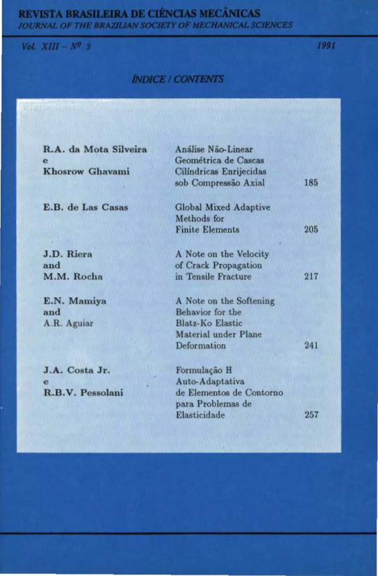
R.A. da Mota Silveira Análise N~Linear e Geométrica de Cascas Khost·ow Ghavami Cilíndricas Enrijecidas

sob Compressão Axial 185

E.B. de Las Casas Global Mixed Adaptive Methods for FiniLe Elements 205

J.D. Riera A Note on the Velocity and of Crack Propagatton M .M. n ocha in Tenstle Fracture 217

E .N. Mamiya A Note on the Soflcning aud Behavtor for lhe A.R. Aguiar Blatz-Ko Elastic

Material under Plane Deformation 241

J.A. Costa Jr. Formulação H e Auto-Adaptativa R.B.V. P cssolani de Elementos de Contorno

para. Problemas de Elasticidade 257