PHYSICAL REVIEW FLUIDS 2, 054608 (2017)

Reynolds number and roughness effects on turbulent stresses in sandpaperroughness boundary layers

C. Morrill-Winter,1 D. T. Squire,1,* J. C. Klewicki,1,2 N. Hutchins,1 M. P. Schultz,3 and I. Marusic1

1University of Melbourne, Victoria 3010, Australia2University of New Hampshire, Durham, New Hampshire 03824, USA

3US Naval Academy, Annapolis, Maryland 21402-5042, USA(Received 21 February 2017; published 26 May 2017)

Multicomponent turbulence measurements in rough-wall boundary layers are presentedand compared to smooth-wall data over a large friction Reynolds number range (δ+).The rough-wall experiments used the same continuous sandpaper sheet as in the study ofSquire et al. [J. Fluid Mech. 795, 210 (2016)]. To the authors’ knowledge, the presentmeasurements are unique in that they cover nearly an order of magnitude in Reynoldsnumber (δ+ � 2800–17 400), while spanning the transitionally to fully rough regimes(equivalent sand-grain-roughness range, k+

s � 37 − 98), and in doing so also maintain verygood spatial resolution. Distinct from previous studies, the inner-normalized wall-normalvelocity variances, w2, exhibit clear dependencies on both k+

s and δ+ well into the wakeregion of the boundary layer, and only for fully rough flows does the outer portion ofthe profile agree with that in a comparable δ+ smooth-wall flow. Consistent with the meandynamical constraints, the inner-normalized Reynolds shear stress profiles in the rough-wallflows are qualitatively similar to their smooth-wall counterparts. Quantitatively, however, atmatched Reynolds numbers the peaks in the rough-wall Reynolds shear stress profiles areuniformly located at greater inner-normalized wall-normal positions. The Reynolds stresscorrelation coefficient, Ruw , is also greater in rough-wall flows at a matched Reynoldsnumber. As in smooth-wall flows, Ruw decreases with Reynolds number, but at differentrates depending on the roughness condition. Despite the clear variations in the Ruw profileswith roughness, inertial layer u, w cospectra evidence invariance with k+

s when normalizedwith the distance from the wall. Comparison of the normalized contributions to the Reynoldsstress from the second quadrant (Q2) and fourth quadrant (Q4) exhibit noticeable differencesbetween the smooth- and rough-wall flows. The overall time fraction spent in each quadrantis, however, shown to be nearly fixed for all of the flow conditions investigated. The dataindicate that at fixed δ+ both Q2 and Q4 events exhibit a sensitivity to k+

s . The presentresults are discussed relative to the combined influences of roughness and Reynolds numberon the scaling behaviors of boundary layers.

DOI: 10.1103/PhysRevFluids.2.054608

I. INTRODUCTION

Turbulent boundary layers over rough walls are of considerable practical interest, since, forexample, most applications involve surfaces that are, or become over time, dynamically rough. Moregenerally, the study of rough-wall turbulence holds potential to provide new insights regarding thepossible effects of the wall boundary condition on wall-turbulence structure. Inquiries into theseeffects are relevant to the dynamics underlying all turbulent wall flows, and especially in connectionwith modifying the mechanisms of wall-normal momentum and scalar transport.

The direct practical importance of high quality rough-wall turbulence measurements, and thebroader issue of flow sensitivities to the wall boundary condition, motivate the present study of

*squired@unimelb.edu.au

2469-990X/2017/2(5)/054608(22) 054608-1 ©2017 American Physical Society

C. MORRILL-WINTER et al.

turbulent stress behaviors in boundary layer flows over smooth and rough walls over comparableReynolds number ranges. The remainder of this Introduction articulates the primary issues to beinvestigated. Throughout, variants of u, v, and w are used to denote the velocity components inthe streamwise (x), spanwise (y), and wall-normal (z) directions, with upper-case symbols denotingmean quantities and an overbar, indicating the application of the time average. Also, a superscript +denotes normalization by inner variables: lengths normalized by ν/Uτ and velocities normalized byUτ , where ν is the kinematic viscosity, and Uτ is the friction velocity.

Surface roughness effects on the mean streamwise velocity profile have been extensively studied,and these effects are generally well-accepted, e.g., Ref. [1]. Clauser [2] and Hama [3] (and manyresearchers since) showed that the streamwise mean velocity profile over a rough wall exhibits aregion of log-linear dependence, as it does in smooth-wall flows. This region is, however, shifteddownward on the profile graph relative to the smooth-wall profile by an amount, �U+, that iscommonly called the roughness function. Physically, the shift indicated by the roughness functionis due to the increased drag of the rough surface. Thus, the mean velocity profile in the logarithmicregion of a rough-wall flow can be expressed as

U+ = 1

κlog(z + ε)+ + A − �U+, (1)

where κ and A are the smooth-wall log-law constants and ε, the zero-plane displacement, accounts forthe roughness itself displacing the entire flow away from the wall. In contrast to current understandingof roughness effects on the mean flow, there is significant uncertainty regarding how rough surfacesaffect turbulence quantities, modify transport mechanisms, or influence the overall structure of theboundary layer. Accordingly, this study complements the recently published investigation of Squireet al. [4], which documented the properties of the mean velocity, U , and streamwise turbulent stress,u2, over a similar range of Reynolds numbers and roughness conditions.

The “k-type” roughness is most associated with flows of practical interest [5]. These includehomogeneously distributed roughness of the kind whose effects are studied herein. Within the k-typeclassification, one can further organize flow behaviors within two regimes that are distinct fromsmooth-wall flows. These regimes depend on the magnitude of �U+ [6]. At finite but sufficientlysmall �U+ (�7), the net drag of the surface derives from a complex mixture of both viscous andpressure effects acting directly on the roughness elements. The flow in this roughness regime istermed transitionally rough. At larger �U+ fully rough flows are observed, whereby the pressuredrag associated with flow separation from the roughness elements dominates the contribution to theoverall drag. The fully rough condition is defined by a �U+ that is a log-linear function of k+,where k is a representation of the roughness height. It is important, however, to note that the fullyrough condition does not necessarily imply that the mean dynamics above the roughness elementsare devoid of a leading order viscous effect [4,7,8].

In rough-wall flow studies it is pragmatic, and thus common practice, to employ Nikuradse’s[9] equivalent sandgrain roughness, ks . This practice forces all fully rough flows to adhere to thelog-linear fully rough asymptote,

�U+ = 1

κlog k+

s + A − A′FR. (2)

The constant A′FR = 8.5 was empirically determined by Nikuradse [9], using a variety of sand

grain roughness surfaces. With this definition, k+s , like �U+, provides a representation of the

rough-wall drag increment relative to the smooth wall, permitting comparisons between flows abovegeometrically different roughnesses.

A large number of rough-wall studies in the existing literature investigate the validity ofTownsend’s wall similarity hypothesis [10]. Here it is hypothesized that at sufficiently high Reynoldsnumber there is an outer flow region, where statistical profiles are unaffected by viscosity, exceptthrough the boundary conditions, which set the velocity scale, Uτ , and the boundary layer thicknesslength scale, δ [1]. Townsend’s hypothesis remains a subject of ongoing investigation, with numerous

054608-2

REYNOLDS NUMBER AND ROUGHNESS EFFECTS ON . . .

studies suggesting its validity [e.g., 11–16], and a smaller but significant number indicating violationsof the hypothesis [e.g., 17–22]. Ramifications associated with the validity of Townsend’s hypothesispertain to the degree that roughness perturbations remain embedded within the turbulence structure,or more broadly, influence the underlying dynamics. By itself, however, the hypothesis is somewhatambiguous relative to addressing these questions, since it speaks fundamentally to statisticalmeasures, and not necessarily to the instantaneous motions that contribute to these measures. Theseconsiderations motivate aspects of the present study to better understand under what conditions andwhy Townsend’s hypothesis is apparently satisfied.

The predominant empirical test for wall similarity is to inner-normalize a given velocity statistic,and then compare smooth- and rough-wall profiles with (z + ε)/δ on the abscissa. Such comparisonsare influenced by errors in Uτ and z, both of which can be difficult to estimate in rough-wall flows. Itis additionally important to keep in mind that the wall similarity hypothesis is based on an asymptotic(high Reynolds number) approximation and pertains to a region beyond where wall perturbationsdirectly affect the flow. Assessing wall similarity is thus further complicated in experiments whereδ+ is low, the roughness geometry generates motions of O(δ) size, or both. Jiménez [6] analyzeddata from a range of extant rough-wall studies and from this suggested that for wall similarity to beoperative, δ/k must be larger than approximately 40. There are, however, studies that do not observewall similarity, even though they satisfy this approximate threshold, e.g., Ref. [23]. Jimenez [6]cites a need for measurements in which δ/k and k+ are both large (low blockage, fully rough flow),and where δ/k is large and k+ is small (low blockage, transitionally rough flow), to help clarifyongoing questions regarding the physics of rough-wall flows. In terms of how the roughness inducedmotions assimilate within the turbulence, such considerations are consistent with recent findings,indicating that the combined roughness and Reynolds number problem is of a richer complexity thancan be adequately captured within the transitionally rough and fully rough characterizations alone[4,7,8,24].

The present investigation complements the recent studies by Squire et al. [4,25,26], whichanalyzed well-resolved streamwise velocity measurements over an unprecedented range of k+

s andδ+ and included u data acquired using the multielement hot-wire sensor of Morrill-Winter et al. [27].In particular, we here extend the rough-wall study of Squire et al. [4] by analyzing the wall-normalvelocity and Reynolds shear stress measurements. This includes comparisons with the smooth-wallmeasurements of Morrill-Winter et al. [27], also acquired with the same sensor and over a comparableReynolds number range. To the authors’ knowledge, the present measurements are unique in thatthey cover nearly an order of magnitude in Reynolds number (δ+ � 2800–17 400) while spanningthe transitionally to fully rough regimes (equivalent sand-grain-roughness range, k+

s � 37 − 98)and in doing so also maintain very good spatial resolution. Per the above discussion, the presentaims include documenting and further clarifying how the combined influences of roughness andReynolds number conspire to produce the net momentum transport and observed statistical featuresof the flow. Throughout the remainder of this paper, x, y, and z denote the streamwise, spanwise,and wall-normal directions, respectively, with z = 0 located at the roughness crest.

II. EXPERIMENTAL DETAILS

The rough-wall measurements were acquired in the flow above P36 grit sandpaper in the highReynolds number boundary layer wind tunnel (HRNBLWT), e.g., Refs. [28,29]. These experimentsare described in Squire et al. [4], and thus only details specific to the present paper are summarizedhere. The sandpaper roughness elevation, h, is normally distributed, with k = 6σ (h) = 0.902 mm andks = 1.96 mm. Multiwire hotwire sensor measurements were acquired at three different streamwiselocations (x ≈ 7 m, 15 m, and 21.7 m), and at three freestream velocities (U∞ ≈ 7 m/s, 12 m/s, and17 m/s). The resulting nine experiments span the range of roughness parameters shown in Fig. 1,and over the friction Reynolds number range 2800 < δ+ < 17 400. The smooth-wall measurementswere obtained in the HRNBLWT and in the Flow Physics Facility (FPF) at the University ofNew Hampshire, and span the Reynolds number range 2600 < δ+ < 12 500 [27]. Table I presents

054608-3

C. MORRILL-WINTER et al.

ΔU

+

k+s

(b)(a)δ/

ks

k+s

20 40 60 80100 1400 50 1000

5

10

0

100

200

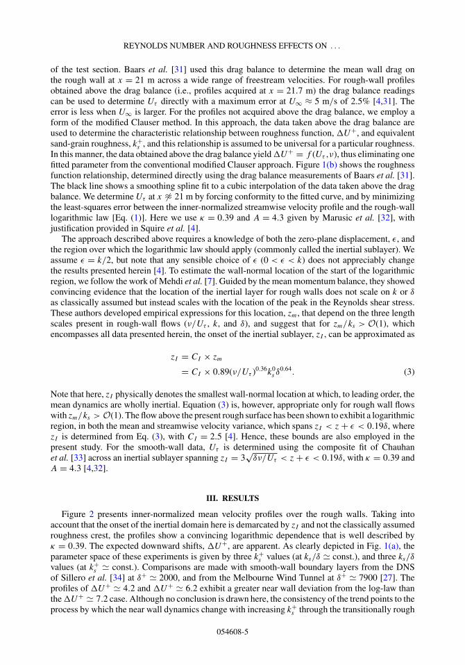
FIG. 1. Visual representation of tabulated parameters. (a) Inner-normalized roughness height versusboundary-layer-roughness-height scale separation. (b) Roughness function as a function of inner normalizedroughness height. Black circles are the profiles coupled with the drag balance; the black line is a smoothingspline fit to a cubic interpolation of the black circles.

properties of the rough-wall boundary layers studied herein. It is noted that here δ is defined as thewall-normal location at which the mean streamwise velocity is 99% of the freestream velocity, U∞.

The multielement hot-wire probe employed is similar to that used by Foss and Haw [30] but isconsiderably smaller. The probe, which consists of a vertical ×-array and two wall-parallel singlewires (all wires have equal length l), is contained within a volume of �x × �y × �z = 0.4 mm ×0.4 mm × 0.5 mm. None of these dimensions exceed 25 wall units across all smooth- and rough-wallmeasurements (see Table I). As described in Morrill-Winter et al. [27], under the current processingthe sensor yields measurements of u, w, uw, and ωy . Here, · represents a total quantity (mean plusfluctuation), and ωy is the spanwise vorticity. (Note that in Morrill-Winter et al. [27] the sensor isreferred to as the ωz probe because they employed y as the wall-normal coordinate.) One novelaspect of the sensor is that the parallel- and cross-wire arrays are interwoven to symmetrically centerthe effective measurement point. A second is its unique calibration and processing scheme thatsolves for w absent its mean value, while independently determining u from the single wires [27].This, for example, results in a greater level of consistency in the Reynolds stress profiles.

The friction velocity, Uτ , is determined for the rough-wall data using the approach describedin Squire et al. [4]. This approach uses the large floating element drag balance that is located inthe Melbourne Wind Tunnel between x = 19.5 m and x = 22.5 m downstream of the beginning

TABLE I. Properties of the rough-wall boundary layers studied herein, as acquired in the HRNBLWT at theUniversity of Melbourne. Also included are the sensor wire length, l+, and wire spacing, �y+. The boundarylayer thickness, δ, is defined as the wall-normal location at which the mean streamwise velocity is 99% of thefreestream velocity, U∞. Note that transitionally rough flows are characterized by k+

s � 70, while fully roughflows are characterized by k+

s � 70.

U∞ uτ ν/uτ l+

symbol δ+ k+s z+

I (m/s) �U+ (m/s) (10−6 m) �z+ �y+

2890 41 365 7.3 4.5 0.314 48.2 10.4 8.55190 38 531 7.2 4.2 0.290 51.5 9.7 8.05250 68 535 12.1 6.3 0.529 28.5 17.5 14.46770 37 629 7.3 4.2 0.287 52.4 9.5 7.87670 97 682 17.1 7.4 0.754 20.1 24.9 20.48980 66 754 12.2 6.1 0.503 29.6 16.9 13.9

12 300 63 922 12.2 6.0 0.488 31.1 16.1 13.213 140 93 962 17.4 7.2 0.718 21.1 23.7 19.417 190 89 1143 17.3 7.1 0.698 21.9 22.9 18.8

054608-4

REYNOLDS NUMBER AND ROUGHNESS EFFECTS ON . . .

of the test section. Baars et al. [31] used this drag balance to determine the mean wall drag onthe rough wall at x = 21 m across a wide range of freestream velocities. For rough-wall profilesobtained above the drag balance (i.e., profiles acquired at x = 21.7 m) the drag balance readingscan be used to determine Uτ directly with a maximum error at U∞ ≈ 5 m/s of 2.5% [4,31]. Theerror is less when U∞ is larger. For the profiles not acquired above the drag balance, we employ aform of the modified Clauser method. In this approach, the data taken above the drag balance areused to determine the characteristic relationship between roughness function, �U+, and equivalentsand-grain roughness, k+

s , and this relationship is assumed to be universal for a particular roughness.In this manner, the data obtained above the drag balance yield �U+ = f (Uτ ,ν), thus eliminating onefitted parameter from the conventional modified Clauser approach. Figure 1(b) shows the roughnessfunction relationship, determined directly using the drag balance measurements of Baars et al. [31].The black line shows a smoothing spline fit to a cubic interpolation of the data taken above the dragbalance. We determine Uτ at x �≈ 21 m by forcing conformity to the fitted curve, and by minimizingthe least-squares error between the inner-normalized streamwise velocity profile and the rough-walllogarithmic law [Eq. (1)]. Here we use κ = 0.39 and A = 4.3 given by Marusic et al. [32], withjustification provided in Squire et al. [4].

The approach described above requires a knowledge of both the zero-plane displacement, ε, andthe region over which the logarithmic law should apply (commonly called the inertial sublayer). Weassume ε = k/2, but note that any sensible choice of ε (0 < ε < k) does not appreciably changethe results presented herein [4]. To estimate the wall-normal location of the start of the logarithmicregion, we follow the work of Mehdi et al. [7]. Guided by the mean momentum balance, they showedconvincing evidence that the location of the inertial layer for rough walls does not scale on k or δ

as classically assumed but instead scales with the location of the peak in the Reynolds shear stress.These authors developed empirical expressions for this location, zm, that depend on the three lengthscales present in rough-wall flows (ν/Uτ , k, and δ), and suggest that for zm/ks > O(1), whichencompasses all data presented herein, the onset of the inertial sublayer, zI , can be approximated as

zI = CI × zm

= CI × 0.89(ν/Uτ )0.36k0s δ

0.64. (3)

Note that here, zI physically denotes the smallest wall-normal location at which, to leading order, themean dynamics are wholly inertial. Equation (3) is, however, appropriate only for rough wall flowswith zm/ks > O(1). The flow above the present rough surface has been shown to exhibit a logarithmicregion, in both the mean and streamwise velocity variance, which spans zI < z + ε < 0.19δ, wherezI is determined from Eq. (3), with CI = 2.5 [4]. Hence, these bounds are also employed in thepresent study. For the smooth-wall data, Uτ is determined using the composite fit of Chauhanet al. [33] across an inertial sublayer spanning zI = 3

√δν/Uτ < z + ε < 0.19δ, with κ = 0.39 and

A = 4.3 [4,32].

III. RESULTS

Figure 2 presents inner-normalized mean velocity profiles over the rough walls. Taking intoaccount that the onset of the inertial domain here is demarcated by zI and not the classically assumedroughness crest, the profiles show a convincing logarithmic dependence that is well described byκ = 0.39. The expected downward shifts, �U+, are apparent. As clearly depicted in Fig. 1(a), theparameter space of these experiments is given by three k+

s values (at ks/δ � const.), and three ks/δ

values (at k+s � const.). Comparisons are made with smooth-wall boundary layers from the DNS

of Sillero et al. [34] at δ+ � 2000, and from the Melbourne Wind Tunnel at δ+ � 7900 [27]. Theprofiles of �U+ � 4.2 and �U+ � 6.2 exhibit a greater near wall deviation from the log-law thanthe �U+ � 7.2 case. Although no conclusion is drawn here, the consistency of the trend points to theprocess by which the near wall dynamics change with increasing k+

s through the transitionally rough

054608-5

C. MORRILL-WINTER et al.

1

1/κ

U+

(z + )+

101 102 103 1045

10

15

20

25

30

FIG. 2. Mean velocity profiles normalized by inner variable. The solid black line is U+ = 0.39−1 log(z+ +ε+) + 4.3 ([32]). Symbols are given in Table I. The black comparison profile is from the DNS of Sillero et al.[34] at δ+ � 2000, and is the δ+ � 7900 smooth wall data presented in Morrill-Winter et al. [27]. Thelarge black symbols show the onset of inertial dynamics, zI , for each profile according to the formulation ofMehdi et al. [7]. Note that transitionally rough flows are characterized by k+

s � 70, while fully rough flows arecharacterized by k+

s � 70.

to fully rough regime. More details on the mean velocity profiles for this experimental campaign aregiven in Squire et al. [4].

A. Turbulent stresses

Statistical profiles associated with the fluctuations of velocity components are often presentedunder an inner-outer normalization to deduce whether the results are in support of Townsend’s

similarity hypothesis [e.g., 35]. The present uw+, w2+

and u2+

profiles are plotted in Figs. 3–5,

respectively. Note that the u2+

profiles were previously discussed and analyzed by Squire et al.[4], but are reproduced here for completeness. Figures 3–5 are not plotted on a linear abscissa, asdoing so tends to imply that the domain of similarity begins at a fixed (z + ε)/δ location. Consistentwith previous studies [4,7,8], the outer similarity argument is considered herein relative to a domainstarting near zI –a position that generally moves to smaller (z + ε)/δ with increasing δ+.

(c)(b)(a)

(z + ) /δ(z + ) /zm(z + )+

−uw

+

102 103 104 100 101 10−1 1000

0.2

0.4

0.6

0.8

1

FIG. 3. Inner-normalized Reynolds stress profile plotted with respect to inner (a), intermediate (b), outernormalized (c) wall position above the rough-wall. The dashed line in (b) shows (z + ε)/zm = 1. The profilesin (c) are only plotted for (z + ε)/δ > zI /δ. Recall zI = 2.5 × zm. Symbols are given in Table I. The blackcomparison profile is the DNS of Sillero et al. [34] at δ+ � 2000, and is the δ+ � 7900 smooth wall datapresented in Morrill-Winter et al. [27].

054608-6

REYNOLDS NUMBER AND ROUGHNESS EFFECTS ON . . .

(c)(b)(a)

(z + ) /δ(z + ) /zm(z + )+

w2+

102 103 104 100 101 10−1 1000

0.5

1

1.5

FIG. 4. Inner-normalized wall-normal velocity variance plotted with respect to inner (a), intermediate (b),outer normalized (c) wall position above the rough-wall. The dashed lines in (b) and (c) show (z + ε)/zm = 1 and(z + ε)/δ = 0.2, respectively. The profiles in (c) are only plotted for (z + ε)/δ > zI /δ. Recall zI = 2.5 × zm.Symbols are given in Table I. The black comparison profile is from the DNS of Sillero et al. [34] at δ+ � 2000,and is the δ+ � 7894 smooth wall data presented in Morrill-Winter et al. [27].

Although the rough-wall Reynolds shear stress profiles of Fig. 3(a) have shapes similar tothose found in smooth-wall flows, relative to inner-normalized wall position, they exhibit a lessrapid near-wall increase. The rough-wall data do, however, monotonically increase to peak at anintermediate wall location (as in smooth-wall flows), and beyond this position they monotonicallydecrease to zero to satisfy the outer boundary condition. Note, that the peak in −uw+ occurs at thelocation, zm, where the Reynolds stress gradient crosses zero. This position can be thought of as asurrogate for where the turbulent inertia transitions from a momentum source to sink [7,36]. The peakmagnitudes of −uw+ are in agreement with −uw+ → 1 as δ+ → ∞, e.g., Ref. [37]. The viscousstress becomes negligible at a small distance from the wall, and as δ+ increases, O(zm) O(ν/Uτ ).This coincides with the formation of a diminishing curvature plateau in the profile over which−uw � U 2

τ . Squire et al. [4] show that the present data adhere to this relationship to within ±2%,thus evidencing a high level of agreement between the present method of estimating the mean wallshear stress, and the peak magnitude of the Reynolds stress.

(c)(b)(a)

(z + ) /δ(z + ) /zm(z + )+

u2+

102 103 104 100 101 10−1 1000

2

4

6

8

FIG. 5. Inner-normalized streamwise velocity variance plotted with respect to inner (a), intermediate (b),outer normalized (c) wall position above the rough-wall. The dashed lines in (b) and (c) show (z + ε)/zm = 1 and(z + ε)/δ = 0.2, respectively. The profiles in (c) are only plotted for (z + ε)/δ > zI /δ. Recall zI = 2.5 × zm.Symbols are given in Table I. The black comparison profile is from the DNS of Sillero et al. [34] at δ+ � 2000,and is the δ+ � 7894 smooth wall data presented in Morrill-Winter et al. [27].

054608-7

C. MORRILL-WINTER et al.

Prevalent descriptions presume that in fully rough flows the maximum of −uw+ is located nearthe crest plane of the roughness. This implies that the totality of the positive Reynolds stress gradientresides within the roughness canopy, regardless of δ+. The total integral of ∂uw+/∂z+ is zero inboth smooth- and rough-wall flows, and thus the positive contribution to the Reynolds stress gradientalways balances the negative portion [7]. The consequences of this are worth exploring in greaterdepth, especially since Squire et al. [4] provide clear evidence that the onset of the log-region for boththe mean and streamwise variance is closely approximated by Eq. (3) (recall zI = CI × zm, wherezm is the wall-normal location of the peak in the Reynolds shear stress). The precise peak locationof −uw+ is challenging to determine with experimental data and especially as δ+ increases. This isbecause the curvature of the Reynolds stress profile, ∂2(−uw+)/∂z+2, diminishes with increasingδ+. Given this, zm was estimated using Eq. (3), and Fig. 3(b) plots −uw+ versus (z + ε)/zm. It isapparent that the (z + ε)/zm coordinate approximately aligns the maxima in −uw+. Admittedly,however, the noted limitations of experimental accuracy only allow a qualitative assessment.

Figure 3(c) plots −uw+ for z + ε � zI against outer normalized wall height. These dataconvincingly support an invariant −uw+ profile on an inertial outer domain (of width that approachesδ as δ+ → ∞) that is specified through consideration of the leading order balances in the meanmomentum equation. As δ+ → ∞, this curve will continue to extend toward zero while increasing inmagnitude to unity. These behaviors are consistent with the classical notion of outer layer similarity,but here the relevant domain is more precisely specified within the context of properties exhibitedby the mean dynamical equation. The net force developed by the Reynolds stress is ∂(−ρuw)/∂z.Therefore, the merging of the Reynolds shear stress profiles observed beyond zI [Fig. 3(c)] indicatesa loss of sensitivity to roughness and Reynolds number. This finding is in line with the similaritythat is observed in the mean velocity profiles in defect form [4].

The wall-normal variance profiles of Fig. 4 exhibit more complicated dependencies on k+s and

δ+ than the Reynolds stress profiles and share some similarities in trend with the streamwisevelocity variance profiles reported in Squire et al. [4]; also see Fig. 9. For the parameter rangesconsidered, a clear k+

s effect is observed in the outer portion of the flow. Although the presentexperiments do not explicitly segregate roughness and friction Reynolds number effects, it is evidentthat as the flow approaches the fully rough regime, the agreement between the smooth- and rough-wall profiles improves. Morrill-Winter et al. [27] found that for smooth-wall flows over 2000 �δ+ � 12 500 the w2

+profiles merge near (z + ε)+ = 80 and for greater (z + ε)+ follow a similar

upward trajectory until (z + ε)/δ � 0.2. Here the profiles attain their peak magnitude and for greater

(z + ε)/δ subsequently decrease to satisfy the outer boundary condition. [Note that hereafter w2+80

refers to w2+

evaluated at (z + ε)+ = 80.] The rough-wall profiles exhibit similar behaviors. Fork+s � 80, however, these profiles exhibit a relative downward shift over the domain (z + ε)+ � 80.

These data also suggest a near wall k+s influence on w2

+, while the observed relative magnitude

increase with increasing (z + ε)+ is apparently preserved. That is, the rate of increase from (z +ε)+ � 80 to (z + ε)/δ � 0.2 remains essentially unchanged. Here we also note that the downwardshift in magnitude is not thought to be a normalization issue (i.e., not a Uτ issue), since the Reynoldsstress profiles exhibit a high level of consistency; also see Ref. [4].

Figure 4(c) plots w2+

under outer-normalization by, once again, only including positions

(z + ε) � zI . This representation reinforces the previous observation that the peaks of the w2+

profiles align at (z + ε)/δ � 0.2. Clearly there is no outer layer similarity for the parameterranges considered here. This observation, however, does not necessarily disagree with the classicalargument. Namely, outer layer similarity may require much higher Reynolds numbers before the

w2+

profile begins to approximate its limiting value. For example, Kunkel and Marusic [38] present

w2+

data for a large range of δ+, including from the atmospheric surface layer. These authors

developed a formulation, guided by their data, that approximates the asymptotic behavior of w2+

.With the criteria used herein and by Squire et al. [4] to detect evidence of outer layer similarity, their

054608-8

REYNOLDS NUMBER AND ROUGHNESS EFFECTS ON . . .

δ+

w2+ m

ax

103 104 105

1.2

1.4

1.6

FIG. 6. The peak magnitude of w2+

with increasing δ+. The rough wall symbols are tabulated in Table I.The open symbols are the smooth-wall data of Morrill-Winter et al. [27] (refer to publication for boundary layerparameters): represent data acquired in the Melbourne Wind Tunnel, where signify data taken in the FPF.The comparison point is from the Sillero et al. [34] DNS at δ+ � 2000. The gray line is the peak functionfrom Kunkel and Marusic [38] and the horizontal black dashed line is the asymptotic limit they gave of 1.78.The black lines represent the least square logarithmic fit for each of the k+

s groupings. These fit lines should besimply considered a visual aid since we have no theoretical reason to suppose that a logarithmic function is theappropriate form for the peak growth.

formulation predicts that similarity is satisfied in smooth-wall flows (to within a small uncertainty)

for δ+ > 105. Squire et al. [4] show that the k+s effect on outer layer similarity for u2

+is only a

weak function of δ+. With this, it seems likely that for the present roughness there is a minimum

δ+(k+s ) threshold at which outer similarity in w2

+is approximated.

To explore this further, Fig. 6 plots the maximum values in w2+

versus friction Reynolds number.For reference, the peak growth function of Kunkel and Marusic [38] is included along with all thesmooth wall data of Morrill-Winter et al. [27], and the highest δ+ data from the DNS of Sillero et al.[34]. The horizontal black dashed line is the asymptotic limit given by Kunkel and Marusic [38]based on Townsend’s [10] attached eddy hypothesis. As is evident, the fully rough data in Fig. 6 trendwith δ+ in a manner similar to the smooth wall case. For the transitionally rough data the growthrate with increasing δ+ does, however, seem to be slightly larger. This behavior is highlighted by thelogarithmic line fitted through the constant k+

s data points (given as the black lines in Fig. 6). Hereit is apparent that the growth rate becomes a decreasing function of k+

s . It is not possible with the

present data to determine conclusively whether the dependency of w2+max on k+

s is lost at sufficientlyhigh δ+, though the results of Fig. 6 provide ostensible evidence that this is indeed the case (certainly,

such behavior is observed for u2+

in the outer region—see Squire et al. [4]). This apparent behavioris consistent with Townsend’s [10] wall-similarity and attached eddy hypotheses.

B. Unravelling roughness and Reynolds number effects

Reynolds shear stress implies the nonzero correlation of u and w. However, both the u2+

profiles

of Squire et al. [4] and the present w2+

profiles exhibit significant dependencies on k+s and δ+.

The trends indicative of these behaviours are captured in Fig. 4 above and Fig. 9 below. Thesetrends are dramatic relative to the more subtle variations exhibited by the uw+ profiles of Fig. 3.Collectively, these observations indicate that the wallward turbulent momentum flux in these flowsvaries considerably relative to the intensities of u and w, and this is reflected in the Reynolds

stress correlation coefficient [Ruw = −uw/(√

u2√

w2)] profiles shown in Fig. 7. Qualitatively, theseprofiles reveal the existence of a clear Reynolds number dependence, and that surface roughnessmodifies this dependence. Of particular note is the (z + ε)/zm normalization (Fig. 7), which shows

054608-9

C. MORRILL-WINTER et al.

(c)(b)(a)

(z + ) /δ(z + ) /zm(z + )+

Ru

w

102 103 104 100 101 10−1 1000

0.1

0.2

0.3

0.4

0.5

FIG. 7. Inner-normalized Reynolds stress correlation coefficient profile plotted with respect to inner (a),intermediate (b), and outer normalized (c) wall position above the rough-wall. The profiles in (c) are onlyplotted for (z + ε)/δ > zI /δ. Recall zI = 2.5 × zm. Symbols are given in Table I. The black comparison profileis from the DNS of Sillero et al. [34] at δ+ � 2000, and is the δ+ � 7894 smooth wall data presented inMorrill-Winter et al. [27].

that the onset of the inertial domain appears to nominally coincide with a local minimum in theRuw profile. (Recall here that zI = CIzm.) Accordingly, under inner and outer normalization, zI ,respectively, moves to increasing (z + ε)+ and decreasing (z + ε)/δ with increasing δ+.

A better understanding of the flow behaviours underlying the profiles of Fig. 3 is gained byclarifying the relative effects of roughness and Reynolds number on the turbulence mechanismfor wall-normal momentum transport. Investigating the behaviors of Fig. 7 is a useful means ofaccomplishing this, since, in essence, Ruw quantifies how efficiently the available turbulence energycontributions combine to affect the turbulence momentum flux. This is a primary aim of the remaininganalyses.

1. Roughness and the logarithmic decay of Ruw with δ+

Using both low Reynolds number wind tunnel data and measurements from the nearly smoothneutrally stratified atmospheric surface layer, the analysis of Priyadarshana and Klewicki [39]revealed that Ruw decreases approximately logarithmically with Reynolds number. The smooth-wallresults of Fig. 8 place this conclusion on much firmer ground by clearly demonstrating that thevalues of Ruw at zI , as well as those of u2 and w2, follow logarithmic variations with δ+ (recallthat zI is approximated differently for smooth- and rough-wall flows; comparisons between smooth-and rough-wall flows at matched (z + ε)/δ are given in the following section). Additionally, thesimilarly plotted rough-wall data reveal that the purely δ+ dependence apparent in the smooth-wallRuw data is unambiguously modified by k+

s influences. The data of Fig. 8(b) indicate that the effectof decreasing k+

s is to increasingly attenuate the underlying growth in u2(zI ) with δ+ such that allof the rough-wall cases exhibit a slower rate of growth than for the smooth-wall. Conversely, theroughness effect on w2(zI ) initially exhibits a steeper slope with increasing δ+ than in smooth-wallflows, but with increasing k+

s the log-linear line becomes approximately parallel to that observed forthe smooth-wall flow. From these observations, one is tempted to surmize that the dependence onδ+ diminishes once k+

s crosses into the fully rough regime. Such a conclusion is, however, deemedpremature. This is because k+

s and δ+ are not independently varied, and once in the fully rough regimethe present data only cover a relatively small δ+ range. Note, that the log-linear fits describing thek+s effects are not theoretically motivated, and thus are included merely to aid in viewing the data

trends. As δ+ → ∞, the outer flow is anticipated (under outer similarity) to become k+s invariant.

054608-10

REYNOLDS NUMBER AND ROUGHNESS EFFECTS ON . . .

δ+

Ru

w(z

I)

103 1040.2

0.3

0.4

0.5

(b)

δ+

u2+

(zI)

103 1043

4

5

6

7

8(c)

δ+

w2+

(zI)

103 1041.1

1.2

1.3

1.4

1.5

1.6

(a)

FIG. 8. Reynolds stress correlation coefficient (a), streamwise velocity variance (b), and wall-normalvelocity variance (c) at the onset of the inertial domain plotted with respect to δ+. The rough wall symbolsare tabulated in Table I. The open symbols are all the smooth-wall data of Morrill-Winter et al. [27] (refer topublication for boundary layer parameters): represent data acquired in the Melbourne Wind Tunnel, wheresignify data taken in the FPF. The comparison point is from the Sillero et al. [34] DNS at δ+ � 2000. Theblack lines represent the least square logarithmic fit for each of the k+

s groupings.

2. Matched Reynolds number comparisons

Extending the analysis of Squire et al. [4] for the streamwise variance, Fig. 9 compares smooth-

and rough-wall u2+

, w2+

, and −uw+ profiles at four approximately matched δ+. The sub-plots ofFig. 9 are ordered from top left to bottom right according to the magnitude of k+

s . By examining flowsat matched Reynolds number, k+

s trends are approximately isolated from those inherent to increasingδ+. It is recognized, however, that the physical interpretation of these comparisons is complicatedby the fact that δ+ is nominally the ratio of largest and smallest scales of motion in the flow, andthus is indirectly influenced by ks through the friction velocity. Similarly, although the value of k+

s

connects to the generation of the wall-shear force (via viscous shear, pressure, or a combination ofthe two), there is ambiguity regarding its direct effect on the overall ratio of scales. As a result, δ+can only be assumed to approximately quantify similar dynamics between comparable δ+ smooth-and rough-wall flows. Thus, the rationale for the comparisons of Fig. 9 is that they provide a nominalmeans of exploring k+

s influences, given an overall condition of scale separation as quantified by δ+.

The w2+

smooth-wall profiles exhibit a relatively abrupt upward near-wall trend. Morrill-Winteret al. [27] showed that this feature correlates with physical wall position, as opposed to inner-normalized distance. They hypothesized that the wall proximity produced a spatial confinement ofthe probe that artificially stimulated the cooling of its ×-array wires. In general, the existing literatureprovides little guidance regarding the characterization of such effects. Morrill-Winter et al. [27] were,

054608-11

C. MORRILL-WINTER et al.

(37, 4)

k+s

ΔU

+

δ+ ≈ 6300 (a)

l+ 9.4l+ 16.3

−uw

+,w

2+

,u2+ 2

0

0.5

1

1.5

2

2.5

3

3.5

4

(41, 5)

k+s

ΔU

+

δ+ ≈ 2700 (b)

l+ 10.2l+ 11.1

(69, 6)

k+s

ΔU

+

(z + )/δ

δ+ ≈ 5500 (c)

l+ 17.4l+ 10.5

−uw

+,w

2+,

u2+ 2

10−3 10−2 10−1 1000

0.5

1

1.5

2

2.5

3

3.5

4(98, 7)

k+s

ΔU

+

(z + )/δ

δ+ ≈ 7800 (d)

l+ 24.6l+ 15.6

10−3 10−2 10−1 100

FIG. 9. Smooth-wall (open symbols) and rough-wall (filled, colored symbols) streamwise velocity variance,wall-normal velocity variance, and Reynolds shear stress comparisons at approximately matched Reynoldsnumbers (shown in the top of each figure). The inset in each figure shows the k+

s and �U+ values of therough-wall data in that figure. The figures are ordered from low k+

s to high k+s . Black dashed lines show

the location corresponding to (z + ε)+ = 80. The large black symbols show the onset of inertial dynamics,zI , for each profile according to the formulation of Mehdi et al. [7]. Note that transitionally rough flows arecharacterized by k+

s � 70, while fully rough flows are characterized by k+s � 70.

however, able to show that this effect seemed to be almost exclusively confined to w2+

, with no

reliably attributable influence on U+, u2+

, and uw+. Interestingly, for the rough-wall experimentsthis effect does not appear to be present. Accordingly, comparisons in Fig. 9 are only considered for(z + ε)+ > 80 (indicated by the black dashed lines in Fig. 9). Relative to objective comparisons, alsonote that, while the present measurements are well-resolved, they do not maintain the same spatialresolution between the rough- and smooth-wall cases. Relative to other experiments of this type, it is

thus unclear how the present slight changes in l+ might effect w2+

or uw+. It is well-documented,however, that at any given wall normal location the length scales associated with w2 are smaller than

those associated with uw, e.g., Ref. [40], and thus the l+ variations are expected to influence w2+

to a greater degree—particularly near the wall. Recent studies have addressed this issue using DNS

simulations, and reported that l+ variations can either amplify or attenuate w2+

—depending on thewall position. Amplification usually occurs for positions close to the wall, and under the conditionof relatively poor spatial resolution, e.g., Ref. [41]. From the present data it is not possible to beprecisely quantitative regarding spatial resolution effects. Given the present l+ values, however, itseems safe to surmize that these effects are likely to be subtle. The l+ values for each of the profilesare noted in Fig. 9.

054608-12

REYNOLDS NUMBER AND ROUGHNESS EFFECTS ON . . .

For all the transitionally rough flows in Fig. 9, differences between the smooth- and rough-wall

w2+

profiles extend well into the wake region. As discussed previously, this seems to be connected

to a decreased amplitude of w2+

at (z + ε)+ ∼ 80 (w2+80); recall that w2

+80 is essentially independent

of δ+ for smooth-wall flows [27]. The rate of increase of w2+

beyond this point also seems tobe the same for both smooth- and rough-wall flows. Interestingly, (z + ε)+ � 70 is the outer limit

of the near-wall cycle for smooth-wall flows [42]. It therefore seems likely that w2+80 is at least

partially determined by the properties of this near-wall cycle, and accordingly, with the addition ofroughness the flow properties in this region are altered. In particular, through the transitionally roughregime the near-wall cycle dynamics are increasingly perturbed, until this cycle is presumably no

longer recognizable in the fully rough regime [6]. The variation of w2+80 depicted in Figs. 9(a)–9(d)

approximately coincides with the perturbation of the near-wall cycle, although the details regardingthe profile behaviors and the specific modifications to the near-wall cycle are currently unknown.

This observation is consistent with the findings presented in Fig. 6 relating to the peak in w2+

.To within the uncertainty of the present experiments, the smooth- and rough-wall Reynolds stress

profiles in Figs. 9(a)–9(d) exhibit remarkable agreement. In particular, this agreement for a fixed δ+appears to hold across the outer domain regardless of k+

s . As mentioned previously, the presenceof a rough-wall causes the onset of inertial mean dynamics to move away from the wall for afixed δ+. Consistent with the formulations and discussion given by Mehdi et al. [7], the relativeinfluences of the three length scales, ν/Uτ , ks , and δ, describe the net behavior of zI . Thus, k+

s

and δ+ are connected to the peak location in −uw+, whereas this position only depends on δ+for smooth wall flows. Figure 9 qualifies this by showing that the rough-wall profiles decrease inmagnitude relative to those in the smooth-wall flows in the region interior to zI of the rough-wall.This is also demonstrated in Fig. 3. The observation is consistent with the generic observation thatz+m(k+

s �= 0) > z+m(k+

s = 0). Also of interest, the −uw+ profiles are very similar between the twodifferent boundary conditions, but for the transitionally rough profiles the ratio, w2/|uw|, is largerfor the smooth-wall flows, and is seemingly not a function of δ+. The results of Figs. 9(a)–9(d)and Ref. [4] indicate that this is similarly the case for u2/|uw|. Such results suggest that, whilethe inner-normalized intensities of the relevant velocity components are attenuated at fixed δ+ forthe rough-wall profiles, their inner-normalized correlation is maintained when compared to thesmooth-wall flow. The finding that −uw+ is similar in smooth- and rough-wall flows at fixed δ+ isconsistent with the mean momentum equation and the curvature of U+ approaching the same valuefor (z + ε) � zI . It is interesting that with the apparent variations in the u and w velocity variances,the motions contributing to these two velocity components organize to preserve their correlation for(z + ε) � zm. Of course, the Reynolds shear stress, uw, is representative of the net wallward flux ofmomentum, which is ultimately reflected by Uτ . Nonetheless, the observation motivates the spectraland quadrant analyses below.

3. Reynolds shear stress co-spectra

An indication of the correlating scales of motion that lead to the Reynolds shear stress profiles inFig. 9 is gained through consideration of the inner-normalized cospectral density of the streamwiseand wall-normal velocity fluctuations (from here on just called the cospectra). Figure 10 presents acomparison of smooth- and rough-wall cospectra throughout the inertial subdomain for the Reynoldsnumbers considered in Fig. 9. Wavelengths were approximated using Taylor’s [43] hypothesisand the local mean velocity. While this is a common approach to estimate a spatial derivativefrom a time series, relative to smooth-wall flows there is less justification for the application ofTaylor’s hypothesis in rough-wall flows since the turbulence intensities as a proportion of the localmean can be significantly larger. Recently, Squire et al. [44] demonstrated that the application ofTaylor’s hypothesis in rough-wall flows can produce erroneous estimates of spectra involving thewall-normal velocity component. We therefore emphasize that prescribing the mean velocity to

054608-13

C. MORRILL-WINTER et al.

(c)(b)(a)−

kxΦ

uw/U

2 τ

λx/(z + )10−2 100 102 10−1 101 103 100 102 104

0

0.05

0.1

0.15

0.2

0.25

FIG. 10. Comparison of smooth- (black lines) and rough-wall (colored lines) cospectra of streamwise andwall-normal velocity fluctuations at approximately matched δ+. Rough-wall profiles are colored as indicatedin Table I. Cospectra are shown at (z + ε) = zI and (z + ε) = 0.19δ for each matched δ+ comparisons, withthe black arrow indicating increasing (z + ε). In (a)–(c), the same comparisons as in Figs. 9(a), 9(c), and 9(d),respectively, are shown (δ+ ≈ 6300,5500,7800).

be the advection velocity for each scale over both wall conditions can, at best, provide only anapproximate representation of wavelength.

According to prevalent theories, once on the inertial domain, the momentum transporting motionsexhibit distance from the wall scaling across a self-similar hierarchy of layers (for example, theLβ hierarchy—see Refs. [45] and [7]—and the attached-eddy hypothesis—see Ref. [46]). In thesmooth-wall case, the relationship from one member of the hierarchy to the next is solely a functionof Reynolds number. In the rough-wall case, the expectation is that the scaling behavior from onehierarchy to the next is, in general, a function of roughness and Reynolds number. Since the influenceof roughness on the hierarchy is not explicitly known, a continuous description of the layer transitionsis beyond our current understanding. We do, however, know that for both smooth- and rough-wallflows the inertial layer begins near zI and ends near (z + ε)/δ = 0.19 (see Ref. [4]). Additionally,Priyadarshana and Klewicki [39] used a filter-based analysis to estimate the predominant frequency(wavelength) contributions to the uw signal. Somewhat contrary to accepted notions, they foundthat even at very high Reynolds numbers these contributions are associated with motions that areintermediate in size relative to the inner and outer scales. Similarly, Ebner et al. [8] observedthat normalizations using zI are effective at bringing statistical profiles from disparate roughnesssurfaces into nominal agreement. With these considerations in mind, Fig. 10 presents cospectra at(z + ε) = zI and (z + ε) = 0.19δ for each matched δ+ comparison. (Recall from Sec. II that zI

is defined differently for the smooth and rough walls; these definitions do not coincide in eitherinner or outer scaling, but instead identify the same mean dynamical condition). To emphasize thedistance from the wall scaling stipulated by the theories just mentioned, the wavelength in Fig. 10 isnormalized by its respective wall-normal location (z + ε).

Given the previously mentioned uncertainties associated with the application of Taylor’shypothesis, the cospectral comparisons in Fig. 10 show inertial region invariance between smooth-and rough-wall flows across all values of k+

s examined. The statistical comparisons in Fig. 9 indicateclear differences in the outer region between the smooth and rough wall streamwise and wall-normalintensities at low k+

s . Yet the apparent invariance of the curves in Fig. 10 suggests that, despite thedifferences in the energy content of the individual velocity component constiuents of the Reynoldsshear stress, the strength and scales of the velocity correlation in the inertial region is somehowmaintained between the smooth- and rough-wall flows. Fully elucidating the above observationsrequires further investigation of the correlating scales of motion that lead to the apparent differencesbetween the smooth and rough wall flow behaviours exhibited in Figs. 7 and 9. On the other hand,Fig. 10 clarifies that, consistent with wall scaling, these differences do not arise from any significant

054608-14

REYNOLDS NUMBER AND ROUGHNESS EFFECTS ON . . .

modifications to the interacting scales of the u and w motions. Insights into the observed differencesare, however, further enabled through quadrant analysis of the Reynolds shear stress correlation.

4. Quadrant analysis

Wallace et al. [47] introduced the conditional analysis of the Reynolds shear stress contributionson the basis of the four possible signed combinations of u and w, referred to as Q1, Q2, Q3, and Q4events. Quadrant analysis provides a useful way to expose the nature of the u and w combinationsthat contribute to uw. Such analysis was particularly relevant in explaining the behaviors observedin the flow visualizations of Grass [48]. These revealed that, above regular gravel-type roughness,violent ejection (Q2) events span much of the wall layer, while the sweep motions (Q4) are confinedto the region close to the wall. In the subsequent literature, there are rough-wall studies that reportan increase [17,49,50], a decrease [14,51], and a negligible change [15,52] in Q2 activity relative tosmooth-wall flow. Similar uncertainty in the effect of roughness is reported relative to Q4 events.Here we present uniformly well-resolved data that enable the conditional structure of the Reynoldsshear stress to be examined over a unique range of parameters. This is particularly pertinent in lightof Fig. 9 showing that at low k+

s the present rough-wall attenuates the inner-normalized streamwiseand wall-normal velocity fluctuations relative to the smooth-wall flow, even though the smooth- andrough-wall uw+ profiles show very good agreement.

A quadrant decomposition using the hyperbolic hole approach of Lu and Willmarth [53] isperformed. Here the percentage contribution to uw from a given quadrant, PQ, is given by

PQ = ProbQ(H ) = limT →∞

1

T uw

∫ T

0uw(t)IQ(t,H )dt. (4)

Here, t represents time, and IQ is an indicator function:

IQ ={

1, when |uw|Q � H√

u2√

w2,

0, otherwise.(5)

The time fraction, TQ, spent in a particular quadrant is computed from

TQ(H ) = 1

T

∫ T

0IQ(t,H )dt. (6)

The hyperbolic hole size, H , sets the magnitude of the threshold for events to be included in theconditional sample with H = 0 corresponding to including all events within a particular quadrant.Figure 11 shows the results of the quadrant analysis for H = 0 (first row) and H = 1 (second row).In Figs. 11(a) and 11(c), each of (i), (ii), and (iii) compares the percentage contribution from Q2and Q4 events to the total Reynolds shear stress above smooth- and rough-wall flows at the threeapproximately matched δ+. The same comparisons as were presented in Figs. 9(a), 9(c), and 9(d)are presented here; recall that the rough-wall profiles are for k+

s = 37, 68, and 97, respectively, butare all at δ+ = 6600 ± 1200.

Figure 11(a) shows that the present rough-wall modifies the u and w structure relative to thesmooth-wall flow. Across all three matched Reynolds number comparisons, the rough-wall appearsto generate a decrease in Q2 activity, while the percentage contribution from Q4 is less affected—especially in the outer region. The Q2 results indicate a reduction in the strength and/or frequencyof ejection events. In Fig. 11(b), the time fractions, T2 and T4, show good agreement between thesmooth- and rough-wall for all three comparisons. This suggests that the smooth/rough differencesin Fig. 11(a) result from modified strength, not frequency, of the Q2 events. This modification alsorequires redistributions of the event amplitude probabilities associated with Q1 and Q3 events, sincethe total percentage from all four quadrants must always sum to 100%.

As demonstrated in Fig. 11(b), neither P2 or P4 show discernible differences between the smooth-wall cases across the present range of friction Reynolds numbers. This supports the notion that (i),

054608-15

C. MORRILL-WINTER et al.

(iii)(ii)(i)

(a)

P2(%

)P

4(%

)

40

60

80

60

80

100

120

T2(%

)T

4(%

)

(b)

26

32

38

44

16

22

28

34

(iii)(ii)(i)

(c)

P2(%

)P

4(%

)

(z + )/δ10−2 10−1 100 10−1 100 10−1 100

0

20

40

6040

60

80

100

120

T2(%

)T

4(%

)

(d)

(z + )/δ10−2 10−1 100

2

6

10

14

2

6

10

14

FIG. 11. Quadrant decomposition of the Reynolds shear stress into percentage contributions from Q2 andQ4 events. The results in the first row [(a) and (b)] are computed using H = 0, while those in the secondrow [(c) and (d)] use H = 1. In (a) and (c), each of (i), (ii), (iii) compares the percentage contribution fromQ2 and Q4 above a smooth-wall (open symbols) and rough-wall (filled, colored symbols) flow at matchedfriction Reynolds number [Reτ ≈ 6300, 5500, and 7800 in (i), (ii), and (iii), respectively]. The roughnessReynolds number of the rough-wall data in these comparisons is k+

s = 37, 68, and 97, respectively. Note thattransitionally rough flows are characterized by k+

s � 70, while fully rough flows are characterized by k+s � 70.

In (b) and (d), all three matched Reynolds number comparisons are plotted to demonstrate trends with k+s . Here,

the percentage contributions from each event (P2 and P4), and the time fractions associated with each event(T2 and T4, respectively) are shown, with the black arrows indicating which data corresponds to which axis.

(ii), and (iii) are sufficiently close in δ+ to approximately isolate trends with k+s . Like for the

smooth-wall flows, the distributions of P2 from the rough-wall experiments appear to be relativelyunaffected by roughness Reynolds number. Conversely, P4 increases across the entire boundary layeras the flow progresses towards the fully rough condition. For H = 1 (second row of Fig. 11), similartrends to those described above are observed, but there are more significant differences betweenthe smooth- and rough-wall Q4 contributions—at least at high k+

s . Note that the H = 1 thresholdisolates only large excursions. Specifically, its use results in the consideration of less than 10% ofthe uw time-series at all wall-normal locations.

T2+4 quantifies the time fraction that uw is producing a wallward flux of momentum. Analysesrevealing self-similar structure admitted by the mean momentum equation suggest that this fraction

054608-16

REYNOLDS NUMBER AND ROUGHNESS EFFECTS ON . . .

(z + )/zI

T2+

4

10−1 100 1010.45

0.5

0.55

0.6

0.65

0.7

0.75

FIG. 12. Time fraction that uv is negative versus wall-normal distance normalized by the onset of inertialdynamics. The rough wall symbols are tabulated in Table I. The open symbols are all the smooth-wall dataof Morrill-Winter et al. [27] (refer to publication for boundary layer parameters): represent data acquiredin the Melbourne Wind Tunnel, where signify data taken in the FPF. The black horizontal lines representT 2+4 = 0.618.

asymptotically approaches a constant value, φ−1c [54]. These analyses also indicate that φ2

c is equal tothe inverse of the leading coefficient in the log law for the mean profile, i.e., one over the von Kármánconstant. Furthermore, under a natural extension to distance from the wall scaling one arrives at theprediction that on the inertial domain φ−1

c = �−1 = 2/(1 + √5) � 0.618, the inverse of the golden

ratio. Relative to the present interest in outer-similarity, it is thus instructive to compare the differingδ+ behaviors of T2+4 for the present variations in k+

s .Figure 12 presents profiles of T2+4 versus (z + ε)/zI . As is apparent, the smooth wall profiles on

this graph attain a convincing plateau on the inertial domain, and the width of this plateau growswith increasing δ+. Also with increasing δ+ (and over the given δ+ range), the plateau value appearsto approach something near to that surmized by Klewicki et al. [54]. The rough-wall data on the

δ+

T2+

4in

ertialsu

bdom

ain

2000 5000 10000

0.6

0.62

0.64

0.66

0.68

FIG. 13. The average time fraction that uw is negative in the inertial domain versus Reynolds number. Therough wall symbols are tabulated in Table I. The open symbols are all the smooth-wall data of Morrill-Winteret al. [27] (refer to publication for boundary layer parameters): represent data acquired in the MelbourneWind Tunnel, where signify data taken in the FPF. The black horizontal lines represent T 2+4 = 0.618.

054608-17

C. MORRILL-WINTER et al.

δ/zI

T2+

4in

ertialsu

bdom

ain

7 10 20

0.6

0.62

0.64

0.66

0.68

FIG. 14. The average time fraction that uw is negative in the inertial domain versus Reynolds numbernormalized by the onset of inertial dynamics. The rough wall symbols are tabulated in Table I. The opensymbols are all the smooth-wall data of Morrill-Winter et al. [27] (refer to publication for boundary layerparameters): represent data acquired in the Melbourne Wind Tunnel, where signify data taken in the FPF.The black horizontal lines represent T 2+4 = 0.618.

plot exhibit a similar trend with δ+. For the given δ+ range, however, T2+4 is consistently larger thanthe smooth-wall flow at comparable δ+. Presuming that an asymptotic value of T2+4 exists, thenrelative to inertial domain momentum transport this value should be reflective of the condition ofouter similarity. This leads to the intriguing observation that the addition of the present roughnessdelays the approach to this asymptotic state. The subject behavior is made clearer in Fig. 13, whichplots the value of T2+4 averaged over the inertial domain versus δ+. From Fig. 12, it also seems clearthat the apparent differences between the smooth- and rough-wall T2+4 profiles near the wall reflectthe direct amplifying effect that roughness has on turbulent momentum transport in this region.

Lastly, we use the result of Fig. 13 to make a broader cautionary observation regarding the notionof scale separation in rough-wall flows. In this figure, the behavior of the rough-wall data seems tosuggest that the approach to the asymptotic state is a slower function of δ+ in the rough-wall flows.Insight into this issue is gained by first noting that δ+ is the ratio of length scales, δ to ν/Uτ . With theaddition of roughness, however, additional length scales are imposed upon, and nonlinearly modify,the scales ranging from O(ν/Uτ ) to O(δ). On average, roughness modifies (generally increases)the position where the flow transitions to inertial mean dynamics. Herein, the characteristic lengthscale of the largest motion affected by a leading order viscous force is estimated by zI . Accordingly,a measure of the scale separation between the characteristic inertial scale and this scale is δ/zI .Figure 14 replots the data of Fig. 13 according to this new measure of scale separation. If theasymptote suggested on Fig. 14 is valid, then the smooth-wall data suggest that a value of δ/zI � 20is required to attain this indicator of self-similar structure on the inertial domain. As is apparent, bythis measure the degree of scale separation is considerably smaller than this in the present rough-wallflows.

IV. CONCLUSIONS

Measurements associated with the turbulent stresses, u2, w2, and uw, were acquired above thesame sandpaper surface that Squire et al. [4] used to study the effects of roughness and Reynoldsnumber on U and u2. The present measurements were acquired using a multielement hot-wiresensing array, and covered a distinctively broad range of Reynolds number and equivalent sand grainroughness 2800 � δ+ � 17 400 and 37 � k+

s � 98, respectively. Numerous comparisons are madebetween these measurements, and those acquired in smooth-wall boundary layers by Morrill-Winteret al. [27] over a comparable δ+ range. To the authors’ knowledge, such comparisons are alsodistinctive in that they involved data from an identical sensor, and these sensors maintained very good

054608-18

REYNOLDS NUMBER AND ROUGHNESS EFFECTS ON . . .

spatial resolution over the entire range of parameters. Important features of the present experimentsare the spatially well-resolved nature of the turbulence measurements, and the direct, and quasidirectmeasurement, of the wall-shear stress. Notably, all of the present profiles show self-consistent trendswith δ+ and k+

s .The mean momentum equation is the same for both smooth- and rough-walled turbulent boundary

layers. Also, the wall-normal gradient of the mean velocity beyond the start of the inertial domainis not influenced by the surface condition. From this, inner-normalized Reynolds stress profiles ata fixed δ+ are not expected to differ in the inertial domain. These features were shown to hold forthe present data. Using the formulation of Mehdi et al. [7], the onset of the inertial domain, zI , wasestimated. When the wall position was normalized by zI , both the smooth- and rough-wall Reynoldsstress peaks seemingly align, thus corroborating the empirical curve-fits of Mehdi et al. [7] for thegiven ks/zI regime. For all of the present measurements, the peak magnitude in −uw+ � 1 andnever exceeded unity. This further reinforced the validity of the approach introduced by Squire et al.[4] to determine Uτ at streamwise locations where drag balance data was not directly available.

When compared to smooth-wall profiles at approximately matched δ+, the present wall-normalvelocity variance profiles in the transitionally rough regime exhibit a reduction in magnitude over thedomain (z + ε)+ � 80. Such behavior is consistent with the gradual roughness-induced perturbationof the near-wall cycle. In particular, the mechanisms of this cycle are expected to diminish as thepressure contribution to the surface drag (due to separated flow around the roughness elements)becomes increasingly large in comparison to the viscous contribution; i.e., as the flow transitionsto the fully-rough regime. Akin to smooth-wall flow behaviors, for increasing positions beyond(z + ε)+ � 80 the present rough-wall profiles exhibit a self-consistent upward trajectory out to

(z + ε)/δ � 0.19. Furthermore, combining this behavior with w2+80 = f (k+

s ) explains the reduced

peak magnitude of w2+

at fixed δ+ for k+s < 70. When the maxima of w2

+are plotted versus δ+,

the fully rough profiles show good agreement with the smooth-wall data, whereas the transitionallyrough data are of lower amplitude. The rate of increase with respect to δ+, however, appears to bean inverse function of k+

s . None of the present transitionally rough-wall data support the validity ofouter similarity over the present δ+ range. Based upon the previous analyses of Kunkel and Marusic[38], these results are interpreted to suggest that the present δ+ are insufficient to approximatelyreflect Townsend’s hypothesis for this statistic in this roughness regime. This result stands in contrastto previous findings pertaining to this statistic.

The rough-wall profiles of Reynolds stress correlation coefficient, Ruw, exhibit elevated valuesrelative to their matched Reynolds number smooth-wall profiles. Like the smooth-wall profiles,however, the rough-wall Ruw exhibit an approximately logarithmic decrease with δ+. The rate oflogarithmic decrement with δ+ varies, however, with k+

s , thus highlighting the combined roughnessand Reynolds number influences on the turbulent flux of momentum. Because the uw+ profilesexhibit only subtle changes between the smooth- and rough-wall flows, the variations in Ruw are

predominantly connected to the individual variations in u2+

and w2+

. Here, the present results

suggest that, increasing k+s flattens the logarithmic increase in u2

+(zI ) (relative to the smooth-wall

case). The same trend is also observed for w2+

(zI ), but in this case the slope does not decreasebelow that of the smooth wall.

The present cospectra of u and w suggest that the inertial layer contributions to uw involve thesame normalized spectral content (range and amplitudes) regardless of k+

s . The distance from thewall normalization required to realize this condition is consistent with the existence of a hierarchicalstructure to inertial layer turbulence, essentially independent of the value of k+

s . The physicalmechanisms that yield the invariant cospectra, despite variations in the spectral content of both u

and w, are presently unknown.Normalized contributions to the Reynolds stress from the second (Q2) and fourth (Q4) quadrants

were evaluated at an approximately fixed δ+ for three different roughness-Reynolds numbercombinations. For all the k+

s values, the Q2 contributions decreased in activity, especially near the

054608-19

C. MORRILL-WINTER et al.

wall, while the Q4 contributions appeared less affected. This result did not substantially change whenthe hyperbolic hole size, H , was increased from 0 to 1. Q4 events, however, were shown to increasein magnitude over the entire boundary layer with increasing k+

s . The present quadrant analysesindicate that, while the inner-normalized Reynolds stress shows similarity over the smooth- andrough-surface, the relevant probabilities underlying the subtly varying uw structure is a complicatedfunction of k+

s and δ+ for the parameter ranges investigated.Finally, the rescaling presented in Fig. 14 raises questions about the validity of matched δ+

comparisons between smooth- and rough-wall flows. The results in Fig. 14 suggest that the ratioδ/zI may provide an alternative view of the true scale separation (and hence an alternative appropriateReynolds number for these flows). The present data are suggestive in this regard, but a wider range ofmatched δ/zI smooth- and rough-wall data are required before informative conclusions can be drawn.

ACKNOWLEDGMENTS

The authors thank the Australian Research Council for the financial support of this research.M.P.S. thanks the US Office of Naval Research for supporting his sabbatical visit to the Universityof Melbourne.

[1] M. R. Raupach, R. A. Antonia, and S. Rajagopalan, Rough-wall turbulent boundary layers, Appl. Mech.Rev. 44, 1 (1991).

[2] F. H. Clauser, Turbulent boundary layers in adverse pressure gradients, J. Aeronaut. Sci. 21, 91 (1954).[3] F. R. Hama, in Boundary-layer Characteristics for Smooth and Rough Surfaces (Trans SNAME, New

York, 1954), pp. 333–351.[4] D. T. Squire, C. Morrill-Winter, N. Hutchins, M. P. Schultz, J. C. Klewicki, and I. Marusic, Comparison of

turbulent boundary layers over smooth and rough surfaces up to high Reynolds numbers, J. Fluid Mech.795, 210 (2016).

[5] A. E. Perry, W. H. Schofield, and P. N. Joubert, Rough wall turbulent boundary layers, J. Fluid Mech. 37,383 (1969).

[6] J. Jiménez, Turbulent flows over rough walls, Annu. Rev. Fluid Mech. 36, 173 (2004).[7] F. Mehdi, J. C. Klewicki, and C. M. White, Mean force structure and its scaling in rough-wall turbulent

boundary layers, J. Fluid Mech. 731, 682 (2013).[8] R. L. Ebner, F. Mehdi, and J. C. Klewicki, Shared dynamical features of smooth- and rough-wall boundary-

layer turbulence, J. Fluid Mech. 792, 435 (2016).[9] J. Nikuradse, Laws of flow in rough pipes, NASA Tech. Memo 361, 1292 (1933).

[10] A. A. Townsend, The Structure of Turbulent Shear Flow (Cambridge University Press, Cambridge, 1976).[11] A. E. Perry and C. J. Abell, Asymptotic similarity of turbulence structures in smooth-and rough-walled

pipes, J. Fluid Mech. 79, 785 (1977).[12] M. R. Raupach, Conditional statistics of Reynolds stress in rough-wall and smooth-wall turbulent boundary

layers, J. Fluid Mech. 108, 363 (1981).[13] M. Acharya, J. Bornstein, and M. P. Escudier, Turbulent boundary layers on rough surfaces, Exp. Fluids

4, 33 (1986).[14] P.-A. Krogstad, H. I. Andersson, O. M. Bakken, and A. Ashrafian, An experimental and numerical study

of channel flow with rough walls, J. Fluid Mech. 530, 327 (2005).[15] K. A. Flack, M. P. Schultz, and T. A. Shapiro, Experimental support for Townsend‘s Reynolds number

similarity hypothesis on rough walls, Phys. Fluids 17, 035102 (2005).[16] R. J. Volino, M. P. Schultz, and K. A. Flack, Turbulence structure in rough-and smooth-wall boundary

layers, J. Fluid Mech. 592, 263 (2007).[17] P.-A. Krogstad, R. A. Antonia, and L. W. B. Browne, Comparison between rough-and smooth-wall

turbulent boundary layers, J. Fluid Mech. 245, 599 (1992).

054608-20

REYNOLDS NUMBER AND ROUGHNESS EFFECTS ON . . .

[18] M. F. Tachie, D. J. Bergstrom, and R. Balachandar, Rough wall turbulent boundary layers in shallow openchannel flow, J. Fluids Eng. 122, 533 (2000).

[19] L. Keirsbulck, L. Labraga, A. Mazouz, and C. Tournier, Surface roughness effects on turbulent boundarylayer structures, J. Fluids Eng. 124, 127 (2002).

[20] S. Leonardi, P. Orlandi, R. J. Smalley, L. Djenidi, and R. A. Antonia, Direct numerical simulations ofturbulent channel flow with transverse square bars on one wall, J. Fluid Mech. 491, 229 (2003).

[21] K. Bhaganagar, J. Kim, and G. Coleman, Effect of roughness on wall-bounded turbulence, Flow Turbul.Combust. 72, 463 (2004).

[22] S.-H. Lee and H. J. Sung, Direct numerical simulation of the turbulent boundary layer over a rod-roughenedwall, J. Fluid Mech. 584, 125 (2007).

[23] V. Efros and P.-A. Krogstad, Development of a turbulent boundary layer after a step from smooth to roughsurface, Exp. Fluids 51, 1563 (2011).

[24] T. Meyers, J. B. Forest, and W. J. Devenport, The wall-pressure spectrum of high-Reynolds-numberturbulent boundary layer flows over rough surfaces, J. Fluid Mech. 768, 261 (2015).

[25] D. T. Squire, C. Morrill-Winter, N. Hutchins, I. Marusic, M. P. Schultz, and J. C. Klewicki, Smooth-andrough-wall boundary layer structure from high spatial range particle image velocimetry, Phys. Rev. Fluids1, 064402 (2016).

[26] D. T. Squire, W. J. Baars, N. Hutchins, and I. Marusic, Inner–outer interactions in rough-wall turbulence,J. Turbul. 17, 1159 (2016).

[27] C. Morrill-Winter, J. Klewicki, R. Baidya, and I. Marusic, Temporally optimized spanwise vorticity sensormeasurements in turbulent boundary layers, Exp. Fluids 56, 1 (2015).

[28] T. B. Nickels, I. Marusic, S. Hafez, and M. S. Chong, Evidence of the k−11 Law in a High-Reynolds-Number

Turbulent Boundary Layer, Phys. Rev. Lett. 95, 074501 (2005).[29] T. B. Nickels, I. Marusic, S. Hafez, N. Hutchins, and M. S. Chong, Some predictions of the attached eddy

model for a high Reynolds number boundary layer, Philos. Trans. R. Soc. A 365, 807 (2007).[30] J. F. Foss and R. C. Haw, Transverse Vorticity Measurements using a Compact Array of Four Sensors,

Symp. on Thermal Anemometry (ASME, New York, 1990).[31] W. J. Baars, D. T. Squire, K. M. Talluru, M. R. Abbassi, N. Hutchins, and I. Marusic, Wall-drag

measurements of smooth- and rough-wall turbulent boundary layers using a floating element, Exp. Fluids.57, 1 (2016).

[32] I. Marusic, J. Monty, M. Hultmark, and A. Smits, On the logarithmic region in wall turbulence, J. FluidMech. 716, R3 (2013).

[33] K. A. Chauhan, P. A. Monkewitz, and H. M. Nagib, Criteria for assessing experiments in zero pressuregradient boundary layers, Fluid Dyn. Res. 41, 021404 (2009).

[34] J. A. Sillero, J. Jiménez, and R. D. Moser, One-point statistics for turbulent wall-bounded flows at Reynoldsnumbers up to δ+ ≈ 2000, Phys. Fluids 25, 105102 (2013).

[35] M. P. Schultz and K. A. Flack, The rough-wall turbulent boundary layer from the hydraulically smooth tothe fully rough regime, J. Fluid Mech. 580, 381 (2007).

[36] T. Wei, P. Fife, J. Klewicki, and P. McMurtry, Properties of the mean momentum balance in turbulentboundary layer, pipe and channel flows, J. Fluid Mech. 522, 303 (2005).

[37] H. Tennekes and J. Lumley, A First Course in Turbulence (MIT Press, Cambridge, MA, 1994).[38] G. J. Kunkel and I. Marusic, Study of the near-wall-turbulent region of the high-Reynolds-number boundary

layer using an atmospheric flow, J. Fluid Mech. 548, 375 (2006).[39] P. J. A. Priyadarshana and J. C. Klewicki, Study of the motions contributing to the Reynolds stress in high

and low Reynolds number turbulent boundary layers, Phys. Fluids 16, 4586 (2004).[40] T. Wei and W. W. Willmarth, Reynolds number effects on the structure of turbulent channel flow, J. Fluid

Mech. 204, 57 (1989).[41] J. Philip, R. Baidya, N. Hutchins, J. P. Monty, and I. Marusic, Spatial averaging of streamwise and

spanwise velocity measurements in wall-bounded turbulence using v-and ×-probes, Meas. Sci. Technol.24, 115302 (2013).

[42] J. Jiménez and A. Pinelli, The autonomous cycle of near-wall turbulence, J. Fluid Mech. 389, 335(1999).

054608-21

C. MORRILL-WINTER et al.

[43] G. I. Taylor, The spectrum of turbulence, in Proc. R. Soc. Lond. A (The Royal Society, London, 1938),Vol. 164, p. 476.

[44] D. T. Squire, N. Hutchins, C. Morrill-Winter, M. P. Schultz, J. C. Klewicki, and I. Marusic, Applicabilityof Taylor’s hypothesis in rough-and smooth-wall boundary layers, J. Fluid Mech. 812, 398 (2017).

[45] J. C. Klewicki, Self-similar mean dynamics in turbulent wall-flows, J. Fluid Mech. 718, 596 (2013).[46] A. E. Perry and I. Marusic, A wall-wake model for the turbulence structure of boundary layers. Part 1.

Extension of the attached eddy hypothesis, J. Fluid Mech. 298, 361 (1995).[47] J. Wallace, H. Eckelmann, and R. Brodkey, The wall region in turbulent shear flow, J. Fluid Mech. 54, 39

(1972).[48] A. J. Grass, Structural features of turbulent flow over smooth and rough boundaries, J. Fluid Mech. 50,

233 (1971).[49] M. P. Schultz and K. A. Flack, Outer layer similarity in fully rough turbulent boundary layers, Exp. Fluids

38, 328 (2005).[50] S. Leonardi, Turbulent Channel Flow with Roughness: Direct Numerical Simulations, Ph.D. thesis,

Universita di Roma (2002).[51] P.-A. Krogstad and R. A. Antonia, Surface roughness effects in turbulent boundary layers, Exp. Fluids 27,

450 (1999).[52] Y. Wu and K. T. Christensen, Outer-layer similarity in the presence of a practical rough-wall topography,

Phys. Fluids 19, 85108 (2007).[53] S. S. Lu and W. W. Willmarth, Measurements of the structure of the Reynolds stress in a turbulent boundary

layer, J. Fluid Mech. 60, 481 (1973).[54] J. C. Klewicki, J. Philip, I. Marusic, K. Chauhan, and C. Morrill-Winter, Self-similarity in the inertial

region of wall turbulence, Phys. Rev. E 90, 063015 (2014).

054608-22