reynolds stress transport modelling of shock …

Pergamon

Compukm & Fluids Vol. 24, No. 3, pp. 253-268. 1995 Copyright 0 1995 Elsevier Science Ltd

00457930(94)ooo38-7 Printed in Great Britain. All rights resewed 0045-7930/95 S9.50 + 0.00

REYNOLDS STRESS TRANSPORT MODELLING OF SHOCK-INDUCED SEPARATED FLOW

LARS DAVIDSON Thermo and Fluid Dynamics, Chalmers University of Technology, S-412 96 Gothenburg, Sweden

(Received 15 November 1993; in revised form 19 October 1994)

Abstract-Predicting the interaction process in transonic flow between the inviscid free stream and the turbulent boundary layer is a challenging task for numerical simulation, which involves complex physical phenomena. In order to capture the physics, a turbulence model capable of accounting for physical phenomena sue h as streamline curvature, strong non-local effects and history effects, and large irrotational strains should be used.

In the present work a second-moment Reynolds Stress Transport Model (RSTM) is used for computing transonic flow in a plane channel with a bump. An explicit time-marching Rung+Kutta code is used for the mean flow <equations. The convecting terms are discretized using a third-order scheme (QUICK), and no explicit dissipation is added. --

For solving the transport equations for the Reynolds stresses u*, v*, and Z as well as k and E an implicit solver is used which-unlike the Runge-Kutta solver-proved to be very stable and reliable for solving source dominated equations. Second-order discretization schemes are used for the convective terms. As the RSTM is valid only for fully turbulent flow, a one-equation model is used near the wall. The two models are matched along a pre-selected grid line in the fully turbulent region.

The agreement between predictions and measurements is, in general, good.

1. INTRODUCTION

Accurate prediction of shock wave turbulent boundary-layer interactions in transonic flows is of great practical importance for many industrial applications. The computers of today are sufficiently powerful to allow us to perform Navier-Stokes calculations on fine grids and-at the same time-use second-moment closure models for the turbulence. When assessing the performance of turbulence models it is important that the configuration is as simple as possible, but that it still possesses the essential details of practical configurations. The shock/boundary-layer interaction in a two-dimensional channel with a bumpwhich is investigated in the present study-fulfils these requirements. This configuration was a test case in a BRITEfEURAM project on CFD-validation called EUROVAL, [ 11.

In the present work, the transonic flow in a two-dimensional channel with a bump is calculated using a Reynolds iStress Transport Model (RSTM), which has been implemented into an existing explicit Runge-Kutta time-marching finite volume code. In order to obtain stable and convergent -- solutions for the equations of the turbulent quantities (k, 6, u2, u* and G), they are solved with an implicit solver. In the viscosity affected flow near the wall (approximately for y + 6 50), the RSTM is matched with a one-equation model.

Second-moment closures such as RSTM are superior to simpler turbulence models such as the k-c or the Baldwin-Lomax models. The main reasons for their superiority are their ability to account for (i) streamline curvature, (ii) strong non-local effects and history effects for the individual stresses, and (iii) irrotational strains, phenomena all of which are present in shock/boundary-layer interaction.

(i) When the streamlines in a boundary layer flow have a convex (concave) curvature turbulence is stabilised (destabilised), which damps (augments) the turbulence [2, 31, especially the shear stress and the Reynolds stress normal to the wall. Bradshaw [2] demonstrates that even small amounts of convex curvature can have a significant effect on the turbulence. In the present configuration both wall curvature and streamline curvature are present.

(ii) The shock produces strong anisotropy in the Reynolds stresses, which is transported downstream.

253

254 Lars Davidson

(iii) In boundary layer flow, the only term which contributes to the production term in the k equation is -pZaU/ay (x denotes streamwise direction). Thompson and Whitelaw [4] found that near the separation point, as well as in the separation zone, the production term - p(u’ - v’) au/ax is of equal importance. This is also the case for transonic flow where large irrotational strains (au/ax, aV/ay) prevail in, for example, the shock region.

The interaction process between the inviscid free stream and the turbulent boundary layer involves complex physical phenomena. When a shock penetrates into a boundary layer, the Mach number of the upstream flow that the shock encounters decreases as the shock approaches the wall. The shock must adapt to this situation so that it vanishes when it reaches sonic conditions. The pressure signal carried by the shock is transmitted in the upstream direction when the Mach number in the inner part of the boundary layer falls below one. Thus, in the inner part of the boundary layer, the information of a sharp pressure increase caused by the shock is transmitted upstream. This causes a thickening of the boundary layer, which generates compression waves in the adjacent supersonic layer. These waves, in turn, weaken the shock. If the shock is strong enough an oblique shock is produced by the coalescence of the compression waves, giving a so-called A-shock.

Up to day, use of second-moment closures in transonic-speed aerodynamics is not too common. Of earlier contributions, those of Vandromme and Haminh [5], Benay et al. [6], Dimitriades and Leschziner [7], Leschziner et al. [8] and Lien and Leschziner [93 should be mentioned. The present methodology-a compressible, time-marching code for the mean flow equations, and an implicit solver for the turbulent quantities-has previously been applied to airfoil flow [IO-121 and to transonic flow in a channel with a bump (incipient separation)

[131. The first part of the paper outlines the numerical method for solving the mean-flow equations,

the second part presents the RSTM. Then follows a section which shows how second-moment closures do respond to streamline curvature effects as well as irrotational strains. The final part presents an extensive comparison of computations and experiments including mean velocities, wall Mach number, and turbulent stresses.

2. MEAN FLOW EQUATIONS

The numerical scheme applied to solve the mean-flow equations is an explicit Runge-Kutta scheme [lo, 14, 151. The mean flow equations in Cartesian coordinates over a control volume I’ with boundary aV read

where the vector of state variables U = (p pU PVPE)~ contains density p, together with x, y components of mean-flow velocity U, V, and energy per unit mass E. The flux tensor 2 is composed of inviscid, viscous and turbulent parts

A?’ = (F, - F, - FT)e,v + (G, - G, - G,)e, (2)

in the x, and y coordinate directions, respectively. The inviscid fluxes are given by

PV

F, = PUV

PV2+P

PVH

(3)

RSTM of shock-induced separated flow 255

and the viscous and turbulent fluxes are given by

I - 0

F,+ FT= z CPU 7 xJ-puV 2

U(~,, - PU2) + w,x - PG I- 4x

Gy+ GT=

H is the stagnation enthalpy, H = E +p/p, and p is the static pressure. The heat flux terms in the energy equation are not calculated with RSTM, but the eddy viscosity

assumption is used., i.e.

qx= -c p LL+$ g ( > t

qy=-cp E+” !x ( ) Pr, ay

where the turbulent viscosity is obtained from k and 6 as

pt=c,,p5 6

The value of the Prandtl number Pr = pep/A was taken as a constant 0.72, and Pr, was set to 0.9 (constant) for the turbulent flow solutions presented in this paper. The laminar viscosity p is calculated using the Sutherland formula. The main reasons why the heat flux terms are computed using the eddy viscosity assumption is that these terms are only weakly involved in the hydrodynamic process. Furthermore, it reduces the complexity of the equation system, avoiding transport equations for another three or four turbulent quantities (q, 2, and maybe the dissipation of temperature fluctuations ct).

The main features of the finite volume code can be summarised as: l explicit, compressible time-marching, cell-centered, local time stepping; . four stage Runge-Kutta scheme for the mean flow equations; . the convective terms in the mean equations are discretized using a third-order scheme

(QUICK) P61; -- o the u2, u2, &, k and 6 equations are solved using an implicit line relaxation solver (TDMA)

[17]; the convective terms are discretized using a second-order scheme of Van Leer [I 81;

2.1. D@erencing scheme

The QUICK scheme [16], i.e. Quadratic Upstream Interpolation Convective Kinematics, utilizes a second-order polynomial fitted to three nodes, two located upstream of the face, and one located downstream; the scheme is thus a form of upwind scheme which can be written, for a uniform grid, as

Qi_+ = -0.125Q,_2 + 0.75&,-, + 0.375Qi, Ui_j > 0

Qi_i = +0.375Qj_, + 0.75&, - 0.125Qi+,, Ui_+ < 0.

where Q is the components of F, and G, in equation (3). The scheme combines accuracy (third-order) with the inherent stability of upwind differencing. This scheme is unbounded, which means that it can give rise to non-physical oscillations. This scheme was implemented into the Rung+Kutta method by Hellstrom [ 11, 121, and it has previously been applied to transonic flow in Ref. [19]. In the:se works QUICK was found to be superior to the other schemes. Generally, the author’s experience is that QUICK is better than second-order schemes; one problem is that it does not always give stable, converged solutions.

The traditional Runge-Kutta method [14, 15,201 is based on central differencing together with explicit adding of second- and fourth-order numerical dissipation, which are tuned with numerical

256 Lars Davidson

premultiplying constants. The present QUICK scheme increases the accuracy and does not involve any tuning numerical constants. The overall accuracy of the method is believed to be close to second-order in space.

2.2. Boundary conditions 2.2.1. Inlet. Total temperature and total pressure are prescribed. V is set to small negligible

values (lo-“) and the density is extrapolated from inside. The U-velocity and the total energy are set as:

E,, = $+)+;w+ V2)

All turbulent quantities are set to zero. The calculations showed to be insensitive to the choice of inlet values on the turbulent quantities, probably because the inlet is located far upstream of the shock. The same experiences were made in Ref. [I].

2.2.2. Outlet. The pressure is fixed at the outlet. For the remaining variables the Riemann invariants are used, which are based on the theory of characteristics for the locally one-dimensional problem. The four Riemann invariants are:

2 R, =U.n--c

Y-l

2 R,=U.n+-c

Y-l

R, = In 0

p PY

R,=n,U -n,V

where n and c denote normal vector and speed of sound, respectively. The normal gradients of the Riemann invariants are set to zero, i.e.

R, is taken from outside and R,, R, and R4 from inside (outside and inside refer to the calculation domain). R, gives the density since the pressure p/p0 is given at the outside. R4 gives the tangential velocity V. Finally, knowing the speed of sound both inside and outside, R, gives the U-velocity.

The streamwise gradients of the turbulence quantities are set to zero. 2.2.3. Wall. The normal gradients for temperature and pressure are set to zero, and the --

remaining variables are set to zero. No boundary conditions are needed for a*, a’, Uv and E, since the one-equation model is used near the walls (see Section 3).

2.2.4. Symmetry line. V and Uu are set to zero, and the normal gradient is set to zero for the remaining variables.

3. THE REYNOLDS STRESS TRANSPORT MODEL

When computing compressible flow either mass-averaging (compressible) or time-averaging (incompressible) variables can be used. In weakly compressible flow (Mach number below 2) as in the present study, the incompressible time-averaging concept can be used.

The Reynolds Stress Transport Model, neglecting compressibility, has the form [21]:

&(p”kuiuj)= -p~~-p~~+~ij+Dij-pe, \ k I I k k I

convection production Pij

(4) + @ij + Dij - PCij


The convection and production terms are exact and do not need any modelling assumptions. The pressure strain Qii and the dissipation cij are modelled in a standard way (see e.g. Gibson and Launder [21]). The diffusion term D, is modelled using the Generalized Gradient Diffusion Hypothesis GGDH [22]

with @ = G. A simpler eddy viscosity assumption

D,= & ”

was also tested. The difference in the obtained results using the two diffusion model was found to be negligible. The constants in the Reynolds stress model are taken from Gibson and Younis [23].

The Reynolds stresses are stored at the cell centres. In implicit SIMPLE codes apparent viscosity is used in the momentum equations to enhance stability via stability-promoting second derivatives [24]. When using Runge-Kutta solvers for the momentum equations, no such stability promoting remedies are needed, because the mean flow variables are solved explicitly, which means that all terms are on the right-hand-side of the discretized equations, and thus the solution procedure is not sensitive to the explicit adding of the Reynolds stresses.

Near the walls the one-equation model by Wolfshtein [25], modified by Chen and Pate1 [26] (see also Ref. [27]), is used. In this model the standard k equation is solved; the diffusion term in the k-equation is modielled using the eddy viscosity assumption. The one-equation model and the RSTM are matched along a pre-selected grid line at approximately y + = 50. The location of the matching line has been varied, and the results were found to be insensitive to the exact location of the matching line. For further details, see Ref. [13]. ---

In an RSTM there are two equivalent sets of equations which can be solved. Either u*, u2, w2, -- E and c or u’, Y*, Ic, Z and t. The latter set has been chosen in the present study. The main reason for this choice that the k-equation has to be solved in the one-equation region under any circumstances.

The standard k and c-equations in the RSTM have the form:

The diffusion terms Dk, D, are, as for the Reynolds stresses, calculated using GGDH, see equation

(9. In Ref. [IO], attempts were made to solve the k and t equations explicitly using the existing

RungeKutta solver. However, no stable, convergent solution was obtained. Instead an implicit

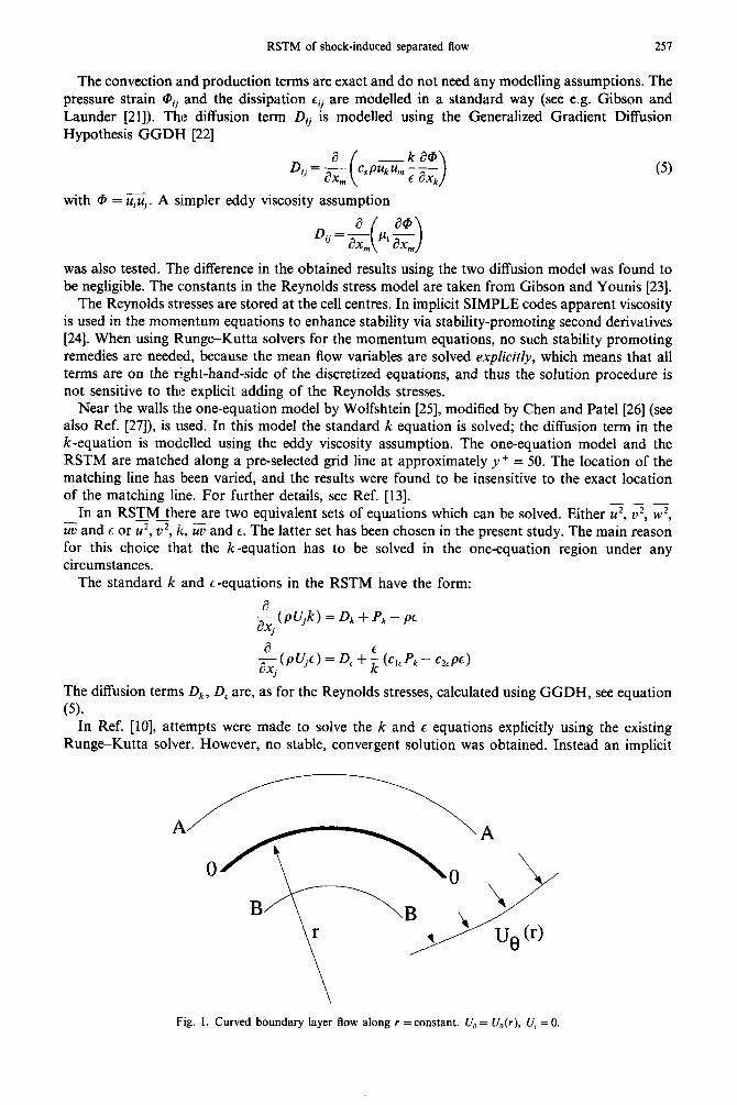
Fig. 1. Curved boundary layer flow along r = constant. U(, = u,,(r), II, = 0.

258 Lars Davidson

discretization method usis an implicit line relaxation solver (TDMA) has been employed for the turbulent quantities (7, v*, Uv, k and c). It has been used for the last 20 years in incompressible codes based on pressure-correction procedures such as SIMPLE [28]. For more details, see Refs. [lo, 171.

Central differencing is employed for the diffusive terms, and for the convective terms a scheme of Van Leer [18] (see also Ref. [13]) is used. The Van Leer scheme is bounded and of second-order accuracy, except at local minima or maxima, where its accuracy is of the first order.

4. THE EFFECTS OF STREAMLINE CURVATURE AND IRROTATIONAL STRAINS

Second-moment closures such as RSTM are superior to simpler turbulence models such as the k-+ and the Baldwin-Lomax models. Two reasons (see Introduction) for the superiority of the RSTM are its ability of taking into account the influence of streamline curvature and normal stresses and irrotational strains. The physics of both these phenomena are faithfully reproduced by second-moment closures because the production terms need not to be modelled.

4.1. Streamline curvature

When the streamlines in a boundary layer flow have a convex curvature the turbulence is stabilised, which damps turbulence [2,3], especially the shear stress and the Reynolds stress normal to the wall. Concave curvature destabilises the turbulence. The ratio of boundary layer thickness 6 to curvature radius R, 6/R, is a common parameter for quantifying the curvature effects on the turbulence. The work reviewed by Bradshaw [2] demonstrates that even such small amounts of convex curvature as 6/R = 0.01 can have significant effects on the turbulence. Thompson and Whitelaw [4] carried out an experimental investigation on a configuration simulating the flow near a trailing edge of an airfoil, where they measured 6/R 2: 0.03. They report a 50% decrease of pv* (Reynolds stress in the normal direction to the wall) due to curvature. The reduction of pu’ and -puU were substantial as well. They also report significant damping of the turbulence in the shear layer in the outer part of the separation region.

Curved boundary layer flow is an illustrative model case. A polar coordinate system r - 0 (see Fig. 1) with 0 locally aligned with the streamline is introduced. As U, = U,(r) (with XJ,/ar > 0 and U, = 0), the inviscid radial momentum equation degenerates to

The centrifugal force exerts a force in the normal direction (outward) on a fluid following the streamline, which is balanced by the pressure gradient. If the fluid is displaced by some disturbance (e.g. turbulent fluctuation) outwards to level A, it encounters a pressure gradient larger than that to which it was accustomed at r = r,, as (U,), > ( Uo)o, which from equation (6) gives (ap/ar), > (ap/Br),. Hence the fluid is forced back to r = ro. Similarly, if the fluid is displaced inwards to level B, the pressure gradient is smaller here than at r = r, and cannot keep the fluid at level B. Instead the centrifugal force drives it back to its original level.

It is clear from the model problem above that convex curvature, when au,/& > 0, has a stabilising effect on (turbulent) fluctuations, at least in the radial direction. How the Reynolds stress model responds to streamline curvature is discussed below.

Assume we have a flat-plate boundary layer flow. The ratio of the normal stresses p2 and pv’ is typically 5. At one x-station the flow is deflected upwards, see Fig. 2. How does this affect the

Y A

streamline

L x -

Fig. 2. The streamlines, which in flat-plate boundary layers are along the x-axis, are suddenly deflected upwards (concave curvature) e.g. due to an approaching shock.


Table 1. Effect of streamline curvature on turbulence

dU.ldr > 0 dU./dr < 0

convex curvature concave curvature

&bilking destabilisinn

destabilising stabilisine

turbulence? Let us study the effect of concave streamline curvature. The production terms P, in equation (4) due to rotational strains can be written

RSTM, z-es.: P,, = -2pu0c ay

RSTM, Z - eq.: p,,= -pss-pg!!! ay

RSTM, 2 - eq.: Pz2 = -2pE g

2

k --L: pk=/Jt

As long as the streamlines in Fig. 2 are parallel to the wall, all production is due to aU/ay, but as soon as the streamlines are deflected we get more terms due to aV/ax. Even if aV/ax is much smaller than aU/a,y it will still give a non-negligible contribution to P,* since pu’ is much larger than pu’. Thus the magnitude of P,2 will increase (P,* is negative) since aV/ax > 0. An increase of the magnitude of P,2 will increase-& which, in turn, will increase P,, and P22. This means that pu’ and p? will be larger and the magnitude of P,, will be further increased, and so on. It is seen that we have positive feedback, which continuously increases the Reynolds stresses. We say that the turbulence is destabilised due to concave curvature of the streamlines.

However, the k--c model is not very sensitive to streamline curvature, since the two rotational strains are multiplied by the same coefficient (the turbulent viscosity).

If the flow in Fig. 2 is a wall-jet flow where aU/ay < 0 the situation will be reversed: the turbulence will be stabilised.

If streamline curvature has a stabilising or destabilising effect is dependent on if momentum in the tangential direction increases or decreases with radial distance from its origo (i.e. the sign of aU,/ar), and on type of curvature (convex or concave). For convenience these cases are summarised in Table 1.

4.2. h-rotational strains

In pure boundary layer flow the only term which contributes to the production term in the k and ~-equations is - pZ aU/ay. Thompson and Whitelaw [4] found that near the separation point, as well as in the separation zone, the production term -p(u’ - u’) dU/ax is of equal importance. As the exact form of the production terms are used in second-moment closures, the production due tat irrotational strains is accounted for correctly.

In the case a,f stagnation-like flow (see Fig. 3), where 2 N 7, the production due to normal stresses is zero, which is also the result given by second-moment closure, whereas k-c

JL Y

I- X

Fig. 3. Stagnation flow.

CAP 241SF

260 Lars Davidson

0.3

Y/L

0.0

0.0 0.5 1 .o 1.5 x/L

Fig. 4. Configuration of the channel with a bump. Left boundary: inlet; right boundary: outlet; upper and lower boundary: wall.

models give large production. In order to illustrate this, let us write the production due to the irrotational strains aU/ax and d V/ay for RSTM and k-c :

RSTM: Pk=0.5(P,,+Pz2)= -pfg-pzz ay

k-t: Pk = :/it{(g)’ + ($y}

If 2 N 2 we get P,, + Pz2 2: 0 since au/ax = -aV/ay due to continuity (nearly incompressible). The production term Pk in k-c model will, however, be large, since it will be sum of the two strains.

5. RESULTS

The configuration is shown in Fig. 4. Grid lines are concentrated in the shock region and near the wall (the first grid line near the wall is located at y+ 2: 2). One advantage of using a one-equation model as compared with using a standard low-Re model where E is solved all the way to the wall, is that the former model does not need as fine a grid near the walls; the latter do need a fine grid in order to resolve the steep gradients of E. Two different grids have been tested, one with 200 x 100 nodes and one with 100 x 147 (see Fig. 5). The predicted results are compared with detailed laser velocimetry data of Dtlery and his group [29, 301 (Case C). The Mach number at the inlet is approx. 0.6. The flow is accelerated over the bump and reaches supersonic conditions with Mu N 1.4 just in front of the shock at x/L 2: 0.94. After the shock the flow separates.

The exit pressure in the experiments wasp,,i,/p, = 0.62. If this value is used, the shock is predicted too late. In order to get a meaningful comparison between different turbulence models, it is important that the shock location is the same for all models. The same conclusion was drawn in EUROVAL [l] and by Dimitriades and Leschziner [7] and Lien [31]. It should be noted that the post-shock pressure is below that given by inviscid theory for a normal shock, which indicates that

Mach

0.600

Fig. 5. Isentropic Mach number at the lower wall.


Y/L

02

0 1’

00 09 1 0

X/L

Fig. 6. (a) Contours of constant Mach numbers. RSTM. (b) Contours of constant Mach numbers in the shock region. RSTM.

the cross-section area is reduced in some way, e.g. by growing boundary layers on the lateral walls causing three-dimensional effects as suggested in Refs [l, 7,311, or, as proposed by Dtlery and Marwin [32], through the rapid increase of the thickness of the boundary layers at the upper and lower walls. The reason for the low pressure after the shock is probably a combination of the two effects. In the calculations the exit pressure has been set to Pe.it/Po = 0.660 for RSTM and 0.670 for kt so as to give the shock at the experimental position.

In Fig. 5 the calculated isentropic Mach number at the wall is compared with experiments. Predictions using two different grids are included, and it can be seen that there is no major difference between the two grids. All results presented below have been obtained with the 200 x loo-mesh. It can be seen that after the shock (x/L 1: 1.5) the predicted Mach number is

0.03

Fig. 7. Displacement thickness. (-) RSTM; (---) k-c.

262 Lars Davidson

smaller (the pressure is larger) than the experimental one. This is because the exit pressure has been increased in the calculations in order to obtain the shock position according to experiments. The experimental values exhibit an increase in the Mach number for x/L > 1.6. This is because there was a contraction in the wind tunnel, which has not been included in the calculations.

Contours of constant Mach numbers are shown in Fig. 6. It can be seen that the shock occurs at x/L 2 0.94 and there is no clear I-structure, indicating a relatively weak interaction between the shock and the turbulent boundary layer. In Fig. 6(b) a zoom presents Mach number contours in the shock region. Here is is clearly seen that the second leg in the I-shock is not captured in the predictions.

In Fig. 7 the predicted displacement thickness is compared with experiments, and it is seen that the predicted interaction is somewhat too weak both with RSTM and k-r, but that after the shock the RSTM-predictions are in better agreement with experiments than are the k+-predictions.

The predicted U-velocities and the Reynolds stresses (divided by density) are compared with experiments in Figs 8 and 9 (all velocities have been made non-dimensional with the stagnation speed of sound a,, and X, y have been made non-dimensional with the length of the bump L). From the U-profiles it is seen that well ahead of the shock (x/L = 0.81) the predicted boundary layer is slightly thinner than the experimental one. The velocity profile at x/L = 0.944 shows that the flow in the lower part of the channel (y/L < 0.05) has entered the shock region, whereas further away from the wall the flow has not yet reached the shock. In the shock region on an airfoil, Alber et al. [33] found similar velocity profiles. This is due to the interaction process between the boundary layer and the external flow. The information of an approaching shock is transmitted upstream in

(4

0.06 -

0.06

0 0 0 1

u/a0

0 0 0 1

u/a0

Fig. 8. U/u,: (-) RSTM; (---) k*. (a) 0, x/L=O.81; w, x/L =0.944; 0, x/L =0.979; 0, x/L = 1.014; x , x/L = 1.049. (b) 0, x/L = 1.084; n , x/L = 1.119; 0, x/L = 1.154;

l , x/L = 1.224; x , x/L = 1.503.


(a) 0 06

0.00

0.06 @I

0.04

Y/L

0.02

0.00

0.06

Cc)

c.04

Y/L

0.02

0.00

0 0 0

-TiiT/a~

0 0.05

0 0 0 0 0.06

G/a;

0 0 F/a:

0 0.005

Fig. 9. Streslr profiles. (a) -Z/u:. (b) s/a:. (c) &I:. (---) RSTM; (---) k+. n , x/L=O.944, 0, x/L = 1.049; 0, x/L = 1.084; 0, x/L = 1.503.

the subsonic part of the boundary layer, which causes a thickening of the boundary layer. This thickening, in turn, generates compression waves in the outer supersonic region. As a result the shock-wave is inclined and the width of the shock region is increased, see Fig. 6.

After the shock, the predicted velocity profiles indicate a weaker tendency of the flow towards separation than is suggested by the experimental data, illustrating a stronger interaction between

264 Lars Davidson

the shock and the turbulent boundary layer in the experiments. This can be due to three- dimensional effects in the experiments. The fact that the predicted boundary layer is thinner (“fuller” velocity profile) ahead of the shock can also affect the tendency towards separation. Generally, velocity profiles with low value of the form factor H,, (“full” boundary layer velocity profiles) has greater resistance to separation as compared with profiles with high H,?. However, this lower resistance to separation for the profiles with high H,, is somewhat increased because the interaction length L* (the distance between the point where the wall pressure starts to rise and the point where the wall Mach number falls to one) increases for increasing H,, [32]. Such an increase in L* leads to a decrease of the adverse pressure gradient, since the supersonic compression takes place over a longer distance, which limits the tendency towards separation.

The velocity profiles in the recovery region show that the predicted recovery rate is too slow as compared with experiments, and the predicted shear stresses are too small (except at the last x station). Comparing the RSTM and the k+ predictions, one finds that the Reynolds stresses obtained from the RSTM are somewhat smaller than those from k-c, although the velocity gradients are larger in the former case, giving a larger production term. This is an example of the sensitivity of the second-moment closure to streamline-curvature-induced damping of turbulence.

The velocity profiles in Fig. 8 show that the recovery rate after the separation region is too slow. It seems that this weakness is worse for RSTM than for k--c, but this is more a result of history effects from the separated region, where the RSTM predicts a larger separation region than k-c. This weakness of the turbulence models has, as pointed out in Ref. [9], also been observed in other flows.

The predicted shear stresses in the shock region are smaller than in the experiments, which seems logical, as the predicted velocity gradients are smaller, thus generating smaller -@-stresses. Turning to the normal Reynolds stresses, it is striking how large is the experimental level of anisotropy in the shock region. It is increasing from z/7 N 5 at x/L = 0.81 to its maximum of 15 at x/L = 1.049, whereas the predicted value (2: 3) is almost unaffected by the shock. The experimental value of 15 is surprisingly high. Delery [29] argues that the cause for the large values of anisotropy can be found by studying the production terms in the 2 and z-equations, which read:

u2 - eq: P,, = -2pUr;c’ - 2pIlig +

G - eq.: P22 = -2pzg - 2pv2~v ay

(7)

In the shock region au/ax is large and negative, which means that the second term in equation (7) increases the production PI, and the second term in equation (8) gives a negative contribution

to p,,, since aV/ay = -all/ax (nearly incompressible) which reduces v2. Hence, the anisotropy should increase at the shock, but the question is whether the increase should be as strong as indicated in the experiments. In Fig. 10 the peak values of u’ E s/a,, and v’ are compared with

72, V'

0.35

0.3

0.25

0.2

0.15

0.1

0.05

0

I I I I 1 I

talc. peak U’ - - talc. peak v’ - -

Fig. IO. Comparison of predicted, using RSTM, and measured peak values of turbulent intensities u’ z (ti2)112/a, and v’.


experiments. The predicted (~‘)r_~ and (a’&_+ increase both rapidly at the shock and seem not to be very much influenced by the normal strains, although they should according to equations (7, 8). In the experiments the maximum of u;,_~ occurs approximately x/L = 0.05 ahead of that of uL,~.

In a later paper by Dtlery and his group [6] they indicate the existence of oscillations of the shock-wave, which act as a turbulence amplifier. These oscillations appear as fluctuations in the x-direction which amplify 2 more than v ‘. However, it should be mentioned that other experimental invesugations also report very high turbulence fluctuations and large anisotropies in the normal stresses. Seegmiller et al. [34] report turbulent kinetic energies of k/a: IV- 0.12 on an airfoil in the immediate post-shock region. Johnson and Bachalo [35], who studied transonic flow -- on a symmetric airfoil, present anisotropies of u2/u2 ‘v 5.8 at 67% of the chord (the shock is located at x/c = 0.37). It is an open question whether this means that shock-oscillations also exist in the experiments presented in Refs. [34,35].

As Cartesian velocity components have been used in the calculations, no explicit curvature terms appear in the Reynolds stress equations [see equation (411. Of course, the Reynolds stresses formulated in Cartesian coordinates are also affected by curvature, but they are affected implicitly. To investigate the curvature effects, it is appropriate to study the equations in polar coordinates r-8, with the flow in the circumferential 8 direction (i.e. U, = Ue(r), U, = 0). The e-axis is thus chosen so that the flow is locally aligned with this axis. Curvature terms now appear because the r = const. coordinate lines are curved. The Reynolds stress equation can, in symbolic form, be written

C, - D, = P, + Qij - cij + P; + C> (9)

where superscript c on P, and C, denotes curvature terms originating from production and convection, respectively, see Table 1. The larger these terms, the more important the curvature effects.

The flux Richardson number

is a convenient parameter for studying curvature effects (for details on how to compute curvature radius of streamlines, see Ref. [36]). Its physical meaning is (minus) the ratio of the production of 2 owing to curvature to the total production of 2 (see Table 2). The ratio 6/R and the flux Richardson numbler are shown in Fig. 11 at three different x stations: at x/L = 0.81 where we have boundary layer flow, after the shock in the separation point (x/L = 0.979) and in the reattachment zone (x/L = 1 .15). As can be seen, the streamline curvature is positive (convex) at x/L = 0.81, which gives an increasing flux Richardson number in the outer part of the boundary layer. The flow here is parallel to the curved wall, which gives constant 6/R, N 0.01, i.e. boundary layer thickness over wall curvature. The boundary layer is very thin, which explains the strong increase in the Richardson flux number at y/L N 0.014, close to the outer edge of the boundary layer. In the separation region, the streamlines bounding the separation region are still convex at x/L = 0.979. Near the point of reattachment the streamlines become concave, which destabilises the turbulence, which is seen in Fig. 11 where 6/R and R, become negative for x/L = 1.15. These values should be compared with reported values on the criticalflux Richardson number (the R,-value at which the turbulence collapse, suppressed by dissipation and buoyancy/curvature effects) in buoyant flows, ranging between 0.15 [37] and 0.5 [38].

Table 2. Source terms in the Reynolds stress equations [see equation (9)] due to production and convection in a polar coordinate system

p,, P; Cf

7 2i;Ti;;s I

2ii;ii;;s I

266 Lam Davidson

(a>

0.00 -

R if

-0.3 0.0 0.3 6/h

Fig. 11. Parameters describing streamline curvature effects on the turbulence. RSTM. (a) Flux

(W

Richardson number R,. (b) Boundary layer thickness over streamline curvature radius 6/R,.

The curvature effects are largest in the outer boundary layer, where the curvature term U,/R becomes comparable with the velocity gradient XJ,,/ar. The direct influence of the curvature effects are thus largest in the outer part of the boundary layer, but they will also have an indirect influence via convective and diffusive transport. The Reynolds stresses, augmented or damped by curvature, increase or decrease the production terms in the equations and, through convection and diffusion, also affect the surroundings.

In Fig. 12 the predicted production terms using RSTM are presented. Note that a wall-oriented s-n coordinate system is used, with s defined along the lower wall. It can be seen that the normal-stress induced production is indeed important in the shock region, where it is larger than that resulting from the shear stresses. The question then arises as to why the k-c model predicts this flow relatively well, even though the model is unable to account for the normal-stress-induced production. One part of the answer lies in the fact that, in the momentum equations, the pressure is the dominating term in the shock region. Another part of the answer can be found in Fig. 12, where the production using the eddy-viscosity assumption is included v,(aU,/an)” (computed from the RSTM flow field). Here it is seen that the inability of the k-+ model to account for the

0.06

0.04

Y/L

0.02

I I I I I I I

0 0 0 0.8

Fig. 12. Comparison of contribution to the production term Pk due to shear and normal stresses. RSTM. The production resulting from the ed_dy vv&cosity assumption is also included. (-) -GdU,/d,;

(---) 424: -u;) avs/as. (----) v,(av,ian)*.


normal-stress induced production is compensated for by overprediction of the shear stresses (and shear-stress induced production). Note that the shear stress -$U,/an used to compute the production in Fig. 12 is larger than that predicted with the k-e model in Fig. 9, since the RSTM flow field (with larger velocity gradients) has been used in Fig. 12.

6. CONCLUSIONS

In the present paper transonic computations of the flow in a plane channel with a bump are performed. The flow at the inlet is subsonic (Ma N 0.6), accelerates over the bump and reaches a maximum Mach number of Ma N 1.4, where a shock occurs. In the interaction region between the shock and the turbulent boundary layer an extended separation region is formed.

A Reynolds Strlzss Transport Model (RSTM) has been implemented into an explicit time- marching Runge-Kutta code. The equations for u , T 2, Uv, k and E, which are solved in an RSTM, are solved using an implicit solver which-unlike the Runge-Kutta solver-has proved to be very stable and reliable when solving these source-dominated transport equations.

The RSTM should be superior to eddy viscosity turbulence models, mainly due to the fact that the production terms need not be modelled. In the paper it is shown that RSTM accounts for streamline curvature effects in a physically correct way, and that it responds properly to large irrotational strains.

Detailed comparisons of predictions, using both RSTM and k-r, and measurements are presented, and the agreement is, in general, good. The interaction between the shock and the boundary layer is stronger in the RSTM-prediction than in the k--E-predictions. The k-c model is shown to handbz this flow fairly well. The reason for this seems to be more due to fortunate circumstances, than to accurate modelling of physical processes. It was found, for example, that in the shock region the contribution in the RSTM to the production stemming from the normal stresses is larger than that from the shear stresses. The inability of the k-6 model to account for normal-stress induced production is (fortuitously) ‘compensated’ for by overprediction of the shear stresses. _ _

The ratio u’/v’ z 15 between the experimental normal stresses in the shock region is surprisingly high; oscillations of the shock-wave observed in the experiments may explain this.

If the conclusion can be drawn that the oscillations in the shock-wave in the experimental flow are of considerable importance, it means, as pointed out in Ref. [6], that a numerical method capable of accounting for these unsteady phenomenon should be used. Using Large Eddy Simulation (LES) methods could be one future way of solving this type of flow.

Acknowledgements--Computer time at the CRAY-XMP at NSC (National Supercomputer Center), Linkijping, Sweden, is gratefully acknowledged.

REFERENCES 1. Euroval, A European initiative on validation of CFD-codes Edited by W. Haase, F. Brandsma, E. Elsholz, M.

Leschziner and D. Schwamborn. Notes on Numerical Fluid Mechanics, Vol. 42. Vieweg Verlag (1993). 2. P. Bradshaw, Effects of streamline curvature on turbulent flow. AGARDograph, No. 169 (1973). 3. W. Rodi, and G. !Scheuerer, Calculation of curved shear layers with two-equation turbulence models. Phys. Fluids 26,

1422 (1983). 4. B. E. Thompson and J. H. Whitelaw, Characteristics of a trailing-edge flow with turbulent boundary-layer separation.

J. Fluid Mech. 157, 305 (1985). 5. P. Vandromme and H. Ha Minh, Physical analysis for turbulent boundary-layer/shock-wave interactions using

second-order closure predictions. Turbulent Shear Flows 4, 127. Springer, Berlin (1985). 6. R. Benay, M. C. Caet, and J. Delery, A study of turbulence modelling in transonic shock-wave boundary-layer

interactions. Turbulent Shear Flows 4, 194. Springer, Berlin (1989). 7. K. P. Dimitriades and M. A. Leschziner, Computation of shock/turbulent-boundary-layer interaction with cell-vertex

method and two-equation turulence model. Proc. R. Aeronautical Society Conference on The Prediction and Exploitation of Separated Flow, pp. 10.1-10.15, London (1989).

8. M. A. Leschziner, K. P. Dimitriades and G. Page. Computational modelling of shock wave/boundary layer interaction with a cell-vertex scheme and transport models of turbulence. Aeronat. .I. R. Aeronat. Sot., 43, Feb. (1993).

9. F. S. Lien, and M . A. Leschziner, A pressure-correction solution strategy for compressible flow and its application to shock/boundary-layer interaction using second-moment turbulence closure. ASME J. Fluid Engng 115, 717 (1993).

10. L. Davidson and .4. Rizzi, Navier-Stokes stall predictions using an algebraic stress model. J. Spacecraft Rockets 29,794 (1992) (see also AIAA-paper 92-0195, Reno, Jan. 1992).

11. Th. Hellstriim, Reynolds stress model transonic flow computations around the RAE 2822 airfoil. Diploma thesis, Rept. 93/3, Therm0 and Fluid Dynamics, Chalmers Univ. of Technology, Gijteborg (1993).

268 Lam Davidson

12.

13.

14. 15.

16.

17.

18.

19.

20.

21.

22. 23. 24.

25.

26.

27.

28. 29.

30. 31.

32. 33.

34. 35.

36.

37. 38.

Th. Hellstrdm, L. Davidson, and A. Rizzi, Reynolds stress transport modelling of transonic around the RAE2822 airfoil, AIAA-paper 94-0309. 3&d AIAA Aerospace Sciences Meeting, Reno (1994). L. Davidson, Reynolds stress transport modelling of shock/boundary-layer interaction, AIAA-paper 93-2936. AIAA 24fh Fluid Dynamics Co& Orlando (1993). A. Rizzi and B. Miiller, Large-scale viscous simulation of laminar vortex flow over a delta wing. AIAA .I. 27,833 (1989). B. Miiller and A. Rizzi, Modelling of turbulent transonic flow around airfoils and wings. Comm. Appl. Nurn. Merh. 6, 603 (1990). B. P. Leonard, A stable and accurate convective modelling based on quadratic upstream interpolation. Comp. M&h. Appl. Mech. Engng 19, 59 (1979). L. Davidson, Implementation of a semi-implicit k-t turbulence model in an explicit Runge-Kutta Navier-Stokes code, TR/RF/90/25. CERFACS, Toulouse, France (1990). B. Van Leer, Towards the ultimate conservative difference scheme. Monotonicity and conservation combined in a second order scheme. J. Comp. Phys. 14, 361 (1974). G. Zhou and L. Davidson, Transonic flow computations using a modified SIMPLE code based on a collocated grid arrangement. Proc. First European Computational Fluid Dynamics Conf., Vol. 2, pp. 749-756, Brussels, 7-11 Sept. (1992). A. Jameson, W. Schmidt and E. Turkel, Numerical solutions of the Euler equations by finite volume methods with Runge-Kutta time stepping schemes, AIAA-paper 8 l- 1259 (198 1). M. M. Gibson and B. E. Launder, Ground effects on pressure fluctuations in the atmospheric boundary layer. J. Fluid Mech. 86, 491 (1978). B. J. Daly, and F. H. Harlow, Transport equations of turbulence. Phys. Fluids 13, 2634 (1970). M. M. Gibson and B. A. Younis, Calculation of swirling jets with a Reynolds stress closure. Phys. Fluids 29, 38 (1986). P. G. Huang, and M. A. Leschziner, Stabilisation of recirculating-flow performed with second-moment closures and third-order discretization. 5th Turbulent Shear Flow, pp. 20.7-20.12, Cornell (1985). M. Wolfshtein, The velocity and temperature distribution in one-dimensional flow with turbulence augmentation and pressure gradient. Inc. .I. Mass Heat Transfer 12, 301 (1969). H. C. Chen, and V. C. Patel, Near-wall turbulence models for complex flows including separation. AIAA I. 26, 641 (1988). W. Rodi, Experience with two-layer models combining the k-t models with a one-equation model near the wall. AIAA-paper 91-0216, Reno (1991). S. V. Patankar, Numerical Heat Transfer and Fluid Flow. McGraw-Hill, New York (1980). J. Delery, Experimental investigation of turbulence properties in transonic shock/boundary-layer interactions. AIAA .I. 21, 180 (1983). J. Delery, M. Sireix and C. Capelier, ONERA. Rapport Technique No. 42/7078 AY 014, Chatillon (1980). F. S. Lien, Computational modelling of 3D flow in complex ducts and passages. PhD thesis, Univ. of Manchester, Manchester (1992). J. Delery and J. G. Marvin, Shock-wave boundary layer interaction (Edited by E. Reshotko.), AGARD-AG-280 (1986). I. E. Alber, J. W. Bacon, B. S. Masson and D. J. Collins, An experimental investigation of turbulent transonic viscous-inviscid interactions. AIAA I. 11, 620 (1973). H. L. Seegmiller, J. G. Marvin and L. L. Levy Jr. Steady and unsteady transonic flow. AIAA J. 16, 1262 (1978). D. A. Johnson and W. D. Bachalo, Transonic flow past a symmetrical airfoil, inviscid and turbulent flow properties. AZAA J. 18, 16 (1980). M. A. Leschziner and W. Rodi, Calculation of annular and twin parallel jets using various discretization schemes and turbulence model variations. J. Fluids Engng, 103, 352 (1981). T. H. Ellison, Turbulent transport of heat and momentum from an infinite rough plane. J. Fluid Mech. 2, 456 (1957). A. A. Townsend, Turbulent flow in stably stratified atmosphere. J. Fluid Mech. 3, 361 (1958).

reynolds stress transport modelling of shock …

Documents