rf measurement assessment of potential wind farm ... · pdf filepage 1 of 87 era business...
TRANSCRIPT

Page 1 of 87
ERA Business Unit: ERA Technology Ltd
Report Title: RF Measurement Assessment of Potential Wind Farm Interference to Fixed Links and Scanning Telemetry Devices
Author(s): B S Randhawa (ERA), R Rudd (Aegis)
Client: Ofcom
ERA Report Number: 2008-0568 (Issue 3)
ERA Project Number: 7G0421901
Report Version: Final Report
ERA Report Checked and Approved by:
Steve Munday
Project Manager, RF Group
March 2009Ref: SPM/vs/62/04219/Rep-6327

ERA Report 2008-0568 (Issue 3)
2
ERA Technology Ltd Cleeve Road Leatherhead Surrey KT22 7SA UK Tel : +44 (0) 1372 367000 Fax: +44 (0) 1372 367099 E-mail: [email protected]
Read more about ERA Technology on our Internet page at: http://www.era.co.uk/
This report describes a technical study undertaken on behalf of the UK regulator, Ofcom, in which a series of measurements were carried out with regard to the presence of wind turbines near to wireless services. The purpose of the study was to enhance understanding of the effects of wind turbines near to wireless services and it is published here for information only. The opinions and conclusions stated in the report are those of ERA Technology Ltd and Aegis Systems Ltd. They may not reflect the view of Ofcom and do not imply any future policy work on the deployment or co-ordination of wind farms.

ERA Report 2008-0568 (Issue 3)
3
Summary
The UK Government is committed to the development of wind energy in the UK through the use of offshore and onshore wind farms. However, concerns have been raised over the effect of wind farms on radiocommunications systems, in particular their impact on fixed links and broadcasting services.
A predecessor body of Ofcom previously initiated a study on establishing an exclusion zone around a path of a fixed radio link within which it would be inadvisable to install a wind turbine [1]. The study identified three principle degradation mechanisms which are relevant to a wind turbine in proximity to a single radio link and presented formulae by which the effects of these mechanisms may be analysed.
In order to consider further this theoretical model, and to enhance understanding of the effects, Ofcom has commissioned ERA Technology Ltd and Aegis Systems Ltd to undertake a series of field trials to measure the effects of wind farms on fixed link and scanning telemetry systems.
Fresnel zone and diffraction measurements
The Fresnel zone and diffraction measurements show that:
• The interference sector behind a single turbine decreases with increasing frequency. This implies that the Fresnel zone decreases with increasing frequency as predicted by diffraction theory.
• A single turbine can produce measured fades as large as 3 dB for UHF scanning telemetry links and 2 dB for fixed links operating between 1.5 and 18 GHz, when the turbine is lying on the transmitter-receiver path and where the wanted link suffers loss in excess of free space. These fades decrease to 1 dB if the turbine 60 m in lateral separation from the link path.
• A wind farm (with seventeen turbines) can produce measured fades as large as 10 to 15 dB for 1% of the time when the wind farm is lying on the transmitter-receiver path and where the wanted link suffers loss in excess of free space. These fades can be as large as 15 to 20 dB for 0.1% of the time, thus reducing the wanted signal by this margin. This in turn will have an affect on the wanted-to-unwanted (W/U) protection ratios for a fixed link or scanning telemetry device. Typically these are 26 to 36 dB for a fixed link and 26 dB for scanning telemetry.
• The fading increases as 10*log10(N) for a wind farm directly situated in the path of the fixed link or scanning telemetry device and where N is the number of turbines for a small sized wind farm. This correlates well with the assumption that the JRC uses in determining the co-ordination zone [3].

ERA Report 2008-0568 (Issue 3)
4
• The measured fades drop to 2 to 3 dB for 1% of the time and 4 dB for 0.1% of the time, for frequencies less than 1 GHz, if the edge of the wind farm (i.e. the outermost turbine) is 625 to 725 m in lateral separation from the link path. Similar reductions in fading were observed for frequencies greater than 1 GHz if the edge of the wind farm is 350 to 625 m in lateral separation from the link path.
• For frequencies below 1 GHz the fading observed at a lateral separation of less than 725 m can be considered as an effect from the edge of a windfarm. For frequencies above 1 GHz the fading observed at a lateral separation of 350 m or less can be attributed to the turbines due to the regularity of the fades with respect to time. These measured lateral separation distances suggest that the co-ordination trigger criteria of 1000 m for frequencies < 1 GHz and 500 m for frequencies > 1 GHz adopted by Ofcom will be valid for fades that occur less than or equal to 0.1% of the time.
The diffraction measurements for the wind farm are summarised in the following table:
Fading observed from multiple wind turbines(dB)
Frequency (MHz)
Lateral Separation (m)
1% of time 0.1% of time
< 1 GHz 0 10 - 15 15 - 20
625 - 725 2 - 3 4
> 1 GHz 0 10 - 12 15 - 18
350 - 625 2 - 3 4
Scattering/reflection measurements
The scattering/reflection results obtained are summarised in the tables below for a single turbine and a wind farm consisting of seventeen turbines.
RCS of a single turbine (dBm²) Frequency (MHz)
Backscatter Intermediate Forward scatter
436 47 26 - 38 53
1477 32 17 - 26 50

ERA Report 2008-0568 (Issue 3)
5
RCS of a wind farm (seventeen turbines) (dBm²) Frequency (MHz) Backscatter Intermediate
(Ivy House) Intermediate (Coldham)
Forward scatter
436 38 31-48 46-53 60
1477 42 20-43 25-42 54
3430 - 22-36 - 41
The main mechanisms observed, by which wind farms may degrade radio link performance, were those of diffraction in the Fresnel zone as well as reflection and scattering from the turbine structure and blades. Such reflected and scattered energy may combine destructively with the direct path signal to give deep nulls in the received power level. The impact of such interference is primarily determined by the relative discrimination afforded by the transmitter and receiver aerials. Furthermore, if the wanted path is obstructed (e.g. due to local clutter or intervening terrain), as can be the case for some scanning telemetry services, the inclusion of a turbine on the transmitter-receiver path between both terminals can cause an increase in interference. This can be attributed to a combination of diffraction effects caused by the local environment and the wind turbine.
It is proposed that the most satisfactory method for predicting the impact of wind turbines on radio systems is to characterise turbines in terms of their radar cross section (RCS), and to apply the bistatic radar equation, taking full account of diffraction and clutter losses on both wanted and reflected paths. This method has the advantage that it is quite general, and can also take full account of radio system parameters such as antenna directivity and required system carrier-to-interference (C/I) ratio.
The primary problem in the application of such a method is that there is little data on the RCS of wind turbines. It is to be expected that the energy reflected from individual turbines will be a function of incidence and scatter angles, the relative yaw of the turbine, the pitch of the blades, and of the frequency. The limited measurements made to date have not been sufficient to do more than indicate a few representative values.
These limited trials have established useful methods for the investigation and characterisation of the impact of wind turbines on radio systems.

ERA Report 2008-0568 (Issue 3)
6
This page is intentionally left blank

ERA Report 2008-0568 (Issue 3)
7
Contents
Page No.
1. Introduction 15
2. Wind Farm Interference 16
2.1 Introduction 16
2.2 Near-Field Effects 17
2.3 Diffraction Effects 17
2.4 Reflection / Scattering Effects 18
2.5 Discussion 20
2.5.1 Scattering effects 20
2.5.2 Determination of RCS 22
2.6 Previous Studies 23
3. Test Site Selection 24
4. Measurement Results 27
5. Summary and Conclusions 27
6. References 30
APPENDIX A 31
A.1 Test Methodology 32
A.1.1 Measurement Approach 32
A.1.2 Measurement Procedure 33
A.2 Single Turbine Measurement Results 35
A.2.1 Measurement Location 35

ERA Report 2008-0568 (Issue 3)
8
A.2.2 Results 36
A.3 Wind Farm Measurement Results 40
A.3.1 Measurement Locations 40
A.3.2 Ivy House Results 42
A.3.3 Four Score Farm 44
A.3.4 Forties Farm 46
A.3.5 Needham Farm 49
A.3.6 Maltmas Drove 51
A.3.7 Gate House 54
A.3.8 White House Farm 56
A.4 Near-field Analysis 58
APPENDIX B 61
B.1 Test Methodology 62
B.1.1 Measurement approach 62
B.1.2 Measurement procedure 63
B.2 Single Turbine Measurement Results 67
B.2.1 Grandford transmit site 67
B.2.2 Percival Farm transmit site 75
B.2.3 Summary 77
B.3 Wind Farm Measurement Results 78
B.3.1 Wind farm – backscatter measurements 80
B.3.2 Wind Farm - Ivy House receive site 80
B.3.3 Wind Farm - Coldham receive site 83
B.3.4 Wind Farm - Needham receive site (forward scatter) 85

ERA Report 2008-0568 (Issue 3)
9
B.3.5 Summary 86
B.4 Conclusions 86
B.4.1 Limitations and further work 87
Tables List
Page No.
Table 1: Wind turbine characteristics................................................................................... 25
Table 2: Transmit and receive antenna parameters ............................................................ 33
Table 3: Transmit and receive cable losses......................................................................... 34
Table 4: Wind farm measurement locations ........................................................................ 40
Table 5: Comparison of calculated and measured received power levels at Ivy House....... 43
Table 6: Comparison of calculated and measured received power levels near Four Score Farm .............................................................................................................................. 46
Table 7: Comparison of calculated and measured received power levels near Forties Farm....................................................................................................................................... 48
Table 8: Comparison of calculated and measured received power levels near Needham Farm .............................................................................................................................. 51
Table 9: Comparison of calculated and measured received power levels at Maltmas Drove....................................................................................................................................... 53
Table 10: Comparison of calculated and measured received power levels at Gate House. 56
Table 11: Comparison of calculated and measured received power levels near White House Farm .............................................................................................................................. 58
Table 12: Calculation of near-field separation distances ..................................................... 59
Table 13: Measurement system characteristics................................................................... 65
Table 14: Summary results for single turbine measurements.............................................. 77

ERA Report 2008-0568 (Issue 3)
10
Table 15: 436 MHz results ................................................................................................... 82
Table 16: 1477 MHz results ................................................................................................. 82
Table 17: 3430 MHz results ................................................................................................. 83
Table 18: 436 MHz results ................................................................................................... 84
Table 19: 1477 MHz results ................................................................................................. 84
Table 20: Summary results for wind farm measurements ................................................... 86
Figures List
Page No.
Figure 1: Approximation to Fresnel zone around a radio path.............................................. 18
Figure 2: Reflection/scattering from wind turbine affecting link between T and R ................ 19
Figure 3: Radar Cross Section.............................................................................................. 21
Figure 4: Forward scatter RCS of idealised turbine blade .................................................... 23
Figure 5: Operational and planned wind farms and power rating, registered with the British Wind Energy Association............................................................................................... 24
Figure 6: Location of turbines used in measurement campaign ........................................... 25
Figure 7: View of single turbine at Long Hill Road ................................................................ 26
Figure 8: View of multiple turbines at Coldham wind farm.................................................... 26
Figure 9: Diagram of Fresnel zone diffraction measurement set-up..................................... 33
Figure 10: Map showing measurement locations along Long Hill Road turbine ................... 36
Figure 11: Sample of a measured time trace showing the wind turbine effects to CW at 436 MHz ............................................................................................................................... 37
Figure 12: Sample of a measured time trace showing the wind turbine effects to CW at 6175 MHz ............................................................................................................................... 37
ERA Report 2008-0568 (Issue 3)
11
Figure 13: CDF of the wanted signal relative to its median with increasing frequency for a single turbine ................................................................................................................. 38
Figure 14: CDF of the wanted 436 MHz signal relative to its median with respect to offset distance from the centre axis......................................................................................... 39
Figure 15: CDF of the wanted 1477 MHz signal relative to its median with respect to offset distance from the centre axis......................................................................................... 39
Figure 16: Map showing measurement locations along Coldhams wind farm...................... 41
Figure 17: Sample of a measured time trace at Ivy House showing the wind farm effects to CW at 436 MHz ............................................................................................................. 42
Figure 18: Sample of a measured time trace at Ivy House showing the wind farm effects to CW at 3430 MHz ........................................................................................................... 42
Figure 19: CDF of the wanted signal relative to its median with increasing frequency as measured at Ivy House.................................................................................................. 43
Figure 20: Sample of a measured time trace near Four Score Farm showing the wind farm effects to CW at 436 MHz.............................................................................................. 44
Figure 21: Sample of a measured time trace near Four Score Farm showing the wind farm effects to CW at 6170 MHz............................................................................................ 44
Figure 22: CDF of the wanted signal relative to its median with increasing frequency as measured near Four Score Farm .................................................................................. 45
Figure 23: Sample of a measured time trace near Forties Farm showing the wind farm effects to CW at 436 MHz.............................................................................................. 46
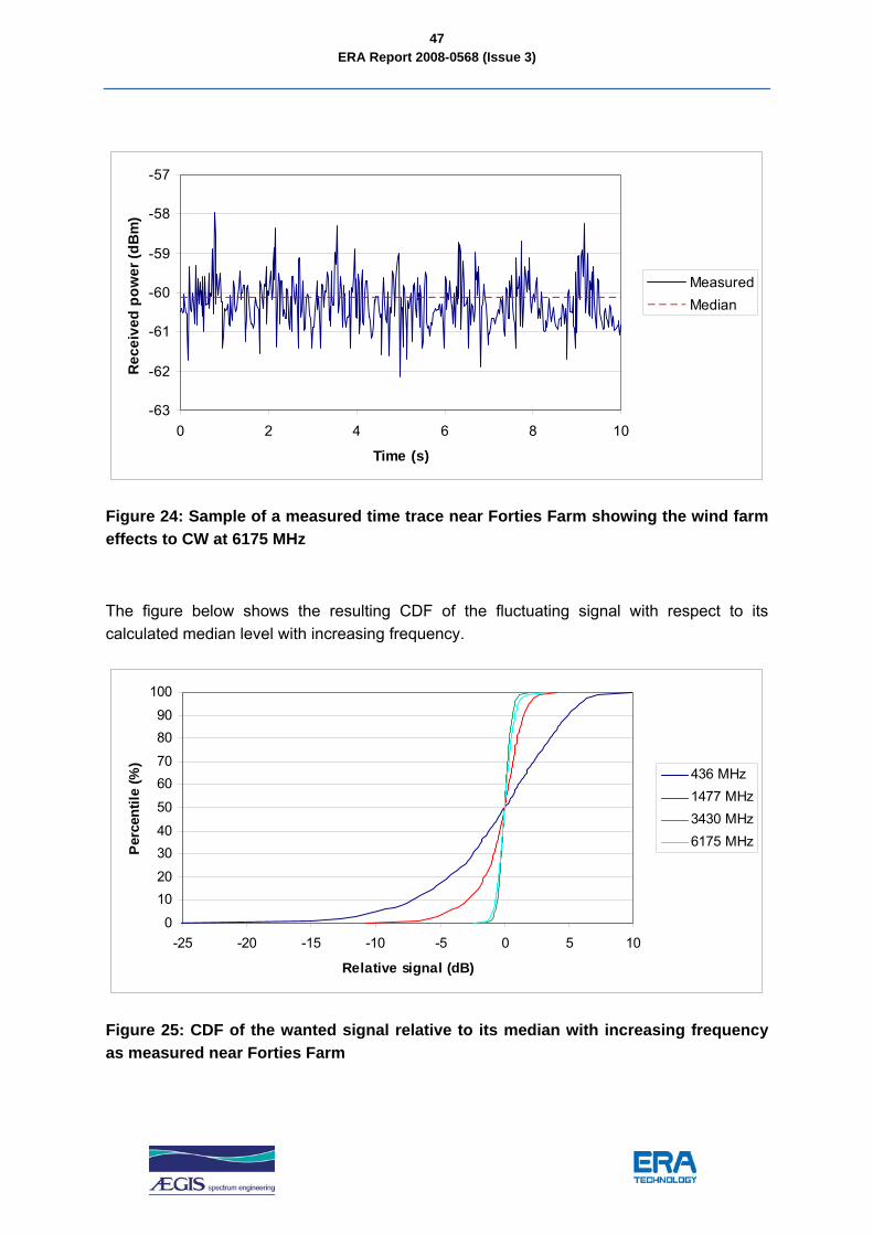
Figure 24: Sample of a measured time trace near Forties Farm showing the wind farm effects to CW at 6175 MHz............................................................................................ 47
Figure 25: CDF of the wanted signal relative to its median with increasing frequency as measured near Forties Farm ......................................................................................... 47
Figure 26: Sample of a measured time trace near Needham Farm showing the wind farm effects to CW at 436 MHz.............................................................................................. 49
Figure 27: Sample of a measured time trace near Needham Farm showing the wind farm effects to CW at 6175 MHz............................................................................................ 49
Figure 28: CDF of the wanted signal relative to its median with increasing frequency as measured near Needham Farm..................................................................................... 50

ERA Report 2008-0568 (Issue 3)
12
Figure 29: Sample of a measured time trace at Maltmas Drove showing the wind farm effects to CW at 1477 MHz............................................................................................ 51
Figure 30: Sample of a measured time trace at Maltmas Drove showing the wind farm effects to CW at 6175 MHz............................................................................................ 52
Figure 31: CDF of the wanted signal relative to its median with increasing frequency as measured at Maltmas Drove.......................................................................................... 52
Figure 32: Sample of a measured time trace at Gate House showing the wind farm effects to CW at 436 MHz ............................................................................................................. 54
Figure 33: Sample of a measured time trace at Gate House showing the wind farm effects to CW at 6175 MHz ........................................................................................................... 54
Figure 34: CDF of the wanted signal relative to its median with increasing frequency as measured at Gate House............................................................................................... 55
Figure 35: Sample of a measured time trace near White House Farm showing the wind farm effects to CW at 436 MHz.............................................................................................. 56
Figure 36: Sample of a measured time trace near White House Farm showing the wind farm effects to CW at 6175 MHz............................................................................................ 57
Figure 37: CDF of the wanted signal relative to its median with increasing frequency as measured near White House Farm................................................................................ 57
Figure 38: Example set of power delay profiles .................................................................... 63
Figure 39: Interior of Aegis Land Rover (receive terminal) ................................................... 64
Figure 40: Interior of ERA Land Rover (transmit terminal).................................................... 64
Figure 41: 436 MHz antenna HRP........................................................................................ 65
Figure 42: 1477 MHz antenna HRP...................................................................................... 66
Figure 43: 3430 MHz antenna pattern .................................................................................. 66
Figure 44: Single Turbine – Grandford transmit site ............................................................. 67
Figure 45: Single Turbine seen from Grandford transmit site (TX on left) ............................ 68
Figure 46: Power delay profiles measured at Grandford, showing intermittent return from traffic .............................................................................................................................. 68

ERA Report 2008-0568 (Issue 3)
13
Figure 47: Backscatter RCS at 1477 MHz ............................................................................ 69
Figure 48: Reflections at Stag’s Holt receiver....................................................................... 70
Figure 49: Near forward scatter paths at ‘Karting’ site.......................................................... 71
Figure 50: Path geometry at 436 MHz .................................................................................. 71
Figure 51: Path geometry at 1477 MHz ................................................................................ 72
Figure 52: CW measurements with path through turbine ..................................................... 73
Figure 53: CW measurements with 50m path clearance ...................................................... 73
Figure 54: CW measurements with 175m path clearance .................................................... 74
Figure 55: Showing frequency selective fading (1477 MHz)................................................. 74
Figure 56: Single Turbine – Percival farm transmit site ........................................................ 75
Figure 57: Single Turbine seen from Graysmore farm receive site ...................................... 76
Figure 58: Sounder response at Graysmore receive site ..................................................... 77
Figure 59: Measurements of Coldham / Stag’s Holt wind farm (Poplar Fm Tx).................... 78
Figure 60: Comparison of sounder response at three frequencies....................................... 79
Figure 61: Intersections of loci of constant delay.................................................................. 79
Figure 62: Ivy House Site looking North West ...................................................................... 81
Figure 63: Aggregate power received by sounder at Needham site (436 MHz) ................... 85

ERA Report 2008-0568 (Issue 3)
14
Abbreviations List
ACAP
Adjacent channel alternate polarisation
ACCP
Adjacent channel co-polarisation
ACP
Adaptive Cellular Plan
BBC
British Broadcast Corporation
BER
Bit Error Ratio
CAA
Civilian Aviation Agency
CCDP
Co-channel dual polar
CDF
Cumulative Distribution Function
C/I
Carrier-to-Interference ratio
MoD
Ministry of Defence
MUS
Minimum Useable Signal
MW
Megawatts
NATS
National Air Traffic Services
QAM
Quadrature Amplitude Modulation
RBW
Resolution Bandwidth
RCS
Radar Cross Section
RPE
Radiation Pattern Envelope
TFAC
Technical Frequency Assignment Criteria
TV
Television
UHF
Ultra High Frequency
W/U
Wanted-to-Unwanted ratio

ERA Report 2008-0568 (Issue 3)
15
1. Introduction
The UK Government is committed to the development of wind energy in the UK through the use of offshore and onshore wind farms. However, concerns have been raised over the effect of wind farms on radiocommunications systems, in particular their impact on fixed links and broadcasting services.
A predecessor body of Ofcom previously initiated a study in an attempt to propose a practical method for establishing an exclusion zone around the path of a fixed radio link within which it would be inadvisable to install a wind turbine [1]. The study identified three principle degradation mechanisms which are relevant to a wind turbine in proximity to a single radio link and presented formulae by which the effects of these mechanisms may be analysed.
In order to consider further this theoretical model, and to enhance understanding of the effects, Ofcom has commissioned ERA Technology Ltd and Aegis Systems Ltd to undertake a series of field trials to measure the effects of wind farms on fixed link and scanning telemetry systems.
It should be noted that a significant amount of theoretical work for a number of radio services has already been performed by other organisations [2][3][4]. In particular, a large amount of work has been performed for radar, including significant amounts of modelling and measurements [5] [6][7]. The MoD, CAA and DTI now have a well established safeguarding pre-planning process for wind farms, following this substantial research.
For other services there has been some modelling and measurements made including scale model laboratory tests and full field trials. In the late 1970’s and 1980’s there was significant interest in interference of wind farms to TV in the US and a significant amount of measurements were made [8] [9].
In the early 1990’s the BBC undertook field tests in Denmark [10], and more recently published a paper with Ofcom on the impact of large buildings and structures (including wind farms) on terrestrial TV reception [11]. A web-based wind farm assessment tool has been developed by the BBC1 to allow the potential impact on TV reception of one or more turbines to be predicted.
1 http://windfarms.kw.bbc.co.uk

ERA Report 2008-0568 (Issue 3)
16
It was not the intention of this study to repeat the earlier work mentioned and therefore the effects of wind farms on broadcasting services and radar have not been considered in this study.
This document describes the findings of the measurements made during field trials to assess the potential interference from wind farms to fixed links and scanning telemetry systems.
2. Wind Farm Interference
This section describes the potential interference effects from wind farms that were taken into account in the measurements by ERA Technology and Aegis Systems.
2.1 Introduction
Reference [1] proposes a method by which an exclusion zone for wind turbines may be determined around a terrestrial fixed radio link. The method takes explicit account of three possible degradation mechanisms:
1. Near-field effects, whereby a transmitting or receiving antenna has a near-field zone where local inductive fields are significant, and within with it is not simple to predict the effect of other objects.
2. Diffraction, whereby an object detrimentally modifies an advancing wave front when it obstructs the wave’s path of travel.
3. Reflection or scattering, whereby the physical structure of the turbines reflects interfering signals into the receiving antenna of a fixed link.
Based on the following statements, the paper presents formulae with which the effects of these mechanisms can be analysed.
• The magnitude of a clearance zone to minimise near-field effects increases with increasing antenna diameter and also increases with increasing link operating frequency.
• The magnitude of a clearance zone to minimise diffraction increases with decreasing link operating frequency.
• The magnitude of a clearance zone to minimise reflection or scattering effects increases with increasing required carrier-to-interference (C/I) ratio for the reflected path and is a function of the antenna discrimination.
ERA Report 2008-0568 (Issue 3)
17
2.2 Near-Field Effects
Where the turbine falls within the near field of a terminal antenna, prediction of the impact on the radio system will be very complex, requiring consideration of inductive as well as radiated fields.
The extent of the near field region ‘d’ for a horn or parabolic antenna can be determined using the following formula:
λη 2Dkd =
Eq. 1
Where, k is constant typically between 1 and 2, η is the antenna efficiency between 0 and 1, D is the diameter of the antenna and λ is the wavelength.
The efficiency of a horn or dish antenna may typically be in the range 0.6 to 0.8. If the value is not known it is conservative to assume that it is 1.0. For other types of antenna where there is no recognisable physical aperture, the near-field distance can be estimated using the effective relationship with gain as:
2πλ
λGkkA
d e ==
Eq. 2
As the near field zones are small, this approach will not present any significant constraint on wind farm deployment.
2.3 Diffraction Effects
Diffraction effects occur when an opaque, or partially opaque, object lies on, or near the radio path. In such cases a “shadow” will exist behind the object, with a predictable interference pattern around it. Given the relative size of typical turbines relative to the Fresnel zone around radio paths, attenuation due to this mechanism will be significant only for higher frequency links with a turbine structure very close to the antenna.
Reference [1] proposes that the criterion for avoiding diffraction effects from wind farms is based on calculating an exclusion zone equal to the 2nd Fresnel zone. The radius RF2 of this zone around the direct line-of-sight path of a radio link is given to an adequate approximation by:

ERA Report 2008-0568 (Issue 3)
18
21
212
2dddd
RF +=
λ
Eq. 3
Where, d1 and d2 are the distances from each end of the radio path.
Figure 1: Approximation to Fresnel zone around a radio path
The figure above illustrates the general form of the zone produced by Equation 3. The definition of Fresnel zone is based upon a fixed path difference between the direct and indirect paths between transmitter T and receiver R, which consists of an ellipse with T and R at the foci. As stated above, Equation 3 is an approximation which clearly fails in the vicinity of the antennas. However this is not important since clearance from the antennas will be covered in any case by the other two criteria.
2.4 Reflection / Scattering Effects
The extent to which an object will reflect or scatter radio waves is usually quantified by its radar cross section (RCS). The RCS value can then be used in the bistatic radar equation (see below) to determine the Carrier-to-Interference (C/I) ratio of a given link geometry.
A fixed radio link is normally designed to different values of C/I. Typically a large C/I is specified, which should be exceeded for all but 20% of time, and a somewhat lower value which must be exceeded for all but a much smaller percentage of time, typically in the range 0.1% to 0.001%. The choice of C/I ratios will depend on the modulation and coding schemes of the link and the required performance. To ensure that a wind turbine has negligible effect on performance it is suggested that the calculation of reflection or scattering should be based on a C/I ratio somewhat higher than the 20% value.

ERA Report 2008-0568 (Issue 3)
19
Figure 2: Reflection/scattering from wind turbine affecting link between T and R
Figure 2 illustrates the geometry used in the assessment of reflection or scattering. The objective is to calculate the C/I ratio between the direct path T-R and the longer path T-W-R reflected or scattered at the wind turbine 'W'. It is assumed that:
1. T and R use directional antennas mutually aligned to maximise the direct T-R signal;
2. The radio link T-R is line of sight, and that in the worst case the paths T-W and W-R are also line of sight;
3. The reflected paths are sufficiently close to the direct path that it can be assumed that any variation of propagation due to atmospheric effects will correlate on both the direct and reflected/scattered paths.
On this basis the calculation of C/I ratio can be based on free-space propagation of the wanted signal along the bore-sight over the free-space propagation of the wanted signal along off the bore-sight.
( ) ( )( ) ( )θθσ
π
212
2121 004ggDggss
IC
p
=
Eq. 4
Where, s1 and s2 are the distances from T to W and W to R, σ is the RCS of the wind turbine, Dp is the radio path distance from T to R and g1 and g2 are the T and R antenna gains.
Equation 4 can be used to calculate the worst-case C/I ratio resulting from a given wind turbine at a known position, which typically would be defined by distances d1, d2 and the side distance Ds in figure 2. If it is wished to draw an exclusion zone around the link it will, in general, be necessary to iterate Equation 4 for increasing values of Ds until the required value of C/I is obtained, and to do this for different pairs of d1 and d2 values along the path.

ERA Report 2008-0568 (Issue 3)
20
Any reflected/scattered signal from the wind turbine outside the zone will arrive at the receiver with an amplitude sufficiently smaller than the direct signal such that its effect, even allowing for the delayed arrival, will be negligible. This calculation is based on the concept of carrier-to-interference ratio (C/I), usually expressed in dB.
Reference [1] notes that there is very little detailed information available on wind turbine RCS values. An obvious problem is that turbines have variable geometry; not only do the blades rotate, but the horizontal axis of blade rotation varies in azimuth according to wind direction, and the pitch angle of the blades varies according to wind speed and electrical load. All these degrees of freedom make measuring the maximum RCS very difficult and in the absence of such information, the proposed algorithm implies that a single, worst-case value of RCS should be used. This may be inappropriate given the very large differences between the forward scatter and backscatter cases, and the scattering from intermediate angles (discussed below).
2.5 Discussion
In the proposed set of algorithms, interference due to the first two mechanisms is to be avoided by applying ‘rule of thumb’ limits. Ensuring that turbine structures lie in the antenna far field, or that they do not obstruct the second Fresnel zone of a link is an appropriate pragmatic solution, but takes no account of specific system parameters, in particular the C/I requirement of the radio link.
The method for determination of interference due to reflection and scattering is potentially more useful, as it attempts to estimate the impact of wind turbine interference to any specific radio system in any specific link geometry. Furthermore, as discussed below, the distinction between diffraction effects and reflection/scattering effects is somewhat artificial and both can be accommodated in the same algorithm.
It is therefore suggested that the ‘bistatic radar’ algorithm for the ‘reflection/scattering’ case should be used generally, to include ‘diffraction’ effects. This will give a model that is both more universal, and at the same time more case-specific. Such a model will, however, require a reliable expression for wind-turbine RCS that is dependant on the bistatic radar angle.
2.5.1 Scattering effects
The quantification of scattering effects in radio systems is generally treated through the concept of RCS. This represents the scattering object in terms of an effective area, the power collected by which would, if re-radiated isotropically, give rise to the observed scattered power.

ERA Report 2008-0568 (Issue 3)
21
Figure 3: Radar Cross Section
The power received at a terminal due to such scattering can be determined using the equation:
22
21
3
2
)4( ddGGPP rtt
r πσλ
=
Eq. 5
Where Pt is the transmitter power, Gt, Gr the gains of the terminal antennas in the direction of the scattering object and d1, d2 the path lengths from transmitter to scatterer and from scatterer to receiver.
Equation 6 is for the more general ‘bistatic’ case, where the terminals are not co-located. Traditional radar systems are generally ‘monostatic’, and have co-located transmitters and receivers using the same antenna. In this case Equation 5 can be simplified to:
Eq. 6
which is the well-known ‘radar equation’. It can be seen from Equation 5 that as the received power is proportional to
22
21
1dd
, the received scattered energy will be at a minimum for a
scatterer near the centre of the path, all other terms being invariant. In practice this conclusion may be significantly modified by the antenna patterns and by the form of the RCS.
43
22
)4( dGP
P tr π
σλ=

ERA Report 2008-0568 (Issue 3)
22
2.5.2 Determination of RCS
The RCS of a scattering object can be determined analytically for only a few simple objects, such as spheres. In general, RCS is determined by measurement (of actual objects, or scale models) or by numerical approximation using Moment Method or other techniques. In the Ofcom paper [1] it is proposed that an RCS equal to the actual projected area of the wind turbine2 be adopted initially, and this is estimated at 30 m2 (15 dB m2).
Monostatic RCS is relatively simple to characterise, involving as it does, only the determination of the backscatter for different orientations of the object. The bistatic case, which will apply for the general geometries associated with interference from wind turbines is more complex, as the RCS will be a function not only of the incidence angle with respect to the turbine, but also of the angular separation of the transmitter and receiver terminals (the bistatic angle) as seen from the turbine. A further complication is that for any orientation and bistatic angle, the RCS will vary with time as the turbine rotates; the turbine blades may also vary in pitch with wind speed, causing further variability in the RCS.
The RCS of objects for bistatic scattering is generally considered as exhibiting three regions. For smooth objects, and small bistatic angles, the RCS can be approximated by the monostatic RCS measured on the bisector of the bistatic angle. Beyond this ‘pseudo-monostatic’ region, the bistatic RCS will generally be smaller than for the monostatic case. The third case is the ‘forward scatter’ region, where the bistatic angle is close to 180°, and the scatterer lies close to the transmit-receive path. This case is clearly of particular interest in the current study.
The mechanism involved in forward scatter is different from the backscatter case, and can be understood from Babinet’s Principle. This principle from optics states the equivalence of the diffraction pattern due to an aperture in a screen or due to an opaque object of the same pattern as the aperture (the principle is often used to explain the operation of slot antennas). For forward scatter RCS, the important point is that the re-radiation behind an opaque (reflecting or absorbing) object such as a turbine will be the same as that from the equivalent aperture.
The power received by the equivalent aperture is proportional to the area, A, while the power
re-radiated is proportional to the aperture’s gain as an antenna, given by 24λπA
. The forward
scatter part of the RCS is therefore given by 2
24λπσ A
F = , and this is plotted below for the
2 As viewed parallel to the axis of blade rotation
ERA Report 2008-0568 (Issue 3)
23
case of an area of 80 m2 (intended to approximate to a single turbine blade of 40 m length by 2 m average width). Also plotted in this diagram is the beamwidth of the forward scatter, which is proportional to wavelength, and inversely proportional to the dimensions of the scatterer. For a wind turbine blade, it is relevant that a vertical blade will concentrate energy in a very narrow vertical beamwidth, while the horizontal pattern will be much broader.
0.1 1 100
20
40
60
80
100
0
5
10
15
20
25RCSBeamwidth (2m)Beamwidth (40m)
RCSBeamwidth (2m)Beamwidth (40m)
Frequency (GHz)
RC
S (d
B m
^2)
3dB
bea
mw
idth
(deg
rees
)
Figure 4: Forward scatter RCS of idealised turbine blade
The primary aim of the Aegis experimental work was to determine values for the radar cross section for typical wind turbines. The results of this work are reported in Annex B.
2.6 Previous Studies
Reference [10] concerns measurements made by a broadcaster of interference to UHF television from a number of wind turbines in Denmark. A site test transmitter was used to establish appropriate test paths. Subjective measurements of picture quality were made, but the principal aim of the study was to quantify the degree of reflection and scattering due to the turbines. This was achieved through recording the interference pattern seen on measurements of received power, and assessing the ratio between the scattered and direct components from the amplitude of the interference pattern. The measured, worst-case, C/I ratios were typically 20-30 dB, which would be problematic for analogue television, but not likely to pose a problem for digital systems.
Reference [4] reports measurements made on an existing UHF link in Northern Ireland. This link (used for electricity company telemetry) suffered significant diffraction loss (>30 dB),

ERA Report 2008-0568 (Issue 3)
24
being obstructed by a hilltop local to one terminal. A wind farm is located on the same hilltop, visible to both terminals of the radio link.
Measurements were made of variability of the received signal level at the terminal local to the wind farm, and a very high degree of fading (up to 40 dB) observed.
The degree of fading experienced is unsurprising given the link geometry. No attempt was made to quantify the relative levels of the direct signal and that scattered from the turbines.
3. Test Site Selection
Wind turbines with a power rating between 0.5 and 2 MW were identified as the preferred candidates for testing, because turbines with this power rating make up the majority of wind farms in current operation. Furthermore, the trend for future development tends to be in the 1 to 2 MW power range as shown in Figure 5 below.
34
4
49
11
24
36
25
33
10
23
9
21
0
7
0
10
20
30
40
50
60
0 to 0.5 0.51 to 1 1.1 to 1.5 1.51 to 2 2.1 to 2.5 2.51 to 3 >3Power rating (MW)
Trend of wind turnbine rating
Non-OperationalOperational
Figure 5: Operational and planned wind farms and power rating, registered with the British Wind Energy Association
Two geographic regions were identified as candidates for measurements in and around March in Cambridgeshire. The flat terrain of this area allowed a range of link-turbine geometries to be investigated with relatively easy access. The characteristics of the wind turbines at the proposed locations are shown in Table 1 below.
ERA Report 2008-0568 (Issue 3)
25
Table 1: Wind turbine characteristics
Site Turbine capacity
Number Maximum Height
Hub height
Rotor diameter
Manufacturer Operator Date
Long Hill Road
2 MW 1 120m 79m+ 82m RE power (MM82)
Wind Direct 2005
Coldham 2 MW 8 100m 60m 80m Vestas (V80) Scottish power / co-op
2006
Stag’s Holt 2 MW 9 100m 60m 80m Vestas V80 E.on 2007
Initial measurements focussed on a single 2 MW wind turbine (Long Hill Road) in an attempt to establish a baseline understanding of the radio properties of these structures. The remainder of the measurements were made on two adjacent wind farms (Coldham and Stag’s Holt) consisting of 8 and 9 turbines, respectively. The locations of these turbines are indicated in Figure 6 below.
Figure 6: Location of turbines used in measurement campaign

ERA Report 2008-0568 (Issue 3)
26
Figure 7: View of single turbine at Long Hill Road
Figure 8: View of multiple turbines at Coldham wind farm
ERA Report 2008-0568 (Issue 3)
27
4. Measurement Results
The test methodology, procedure and results for near-field and diffraction effects from wind turbine(s) described in Section 2 and measured by ERA Technology can be found in Appendix A.
The test methodology, procedure and results for reflection/scattering effects from wind turbine(s) described in Section 2 and measured by Aegis Systems can be found in Appendix B.
5. Summary and Conclusions
A predecessor body of Ofcom previously initiated a study in an attempt to propose a practical method for establishing an exclusion zone around the path of a fixed radio link within which it would be inadvisable to install a wind turbine [1]. The study identified three principle degradation mechanisms which are relevant to a wind turbine in proximity to a single radio link and presented formulae by which the effects of these mechanisms may be analysed.
In order to consider further this theoretical model, and to enhance understanding of the effects, Ofcom has commissioned ERA Technology Ltd and Aegis Systems Ltd to undertake a series of field trials to measure the effects of wind farms on fixed link and scanning telemetry systems.
Fresnel zone and diffraction measurements
The Fresnel zone and diffraction measurements show that:
• The interference sector behind a single turbine decreases with increasing frequency. This implies that the Fresnel zone decreases with increasing frequency as predicted by diffraction theory.
• A single turbine can produce measured fades as large as 3 dB for UHF scanning telemetry links and 2 dB for fixed links operating between 1.5 and 18 GHz, when the turbine is lying on the transmitter-receiver path and where the wanted link suffers loss in excess of free space. These fades decrease 1 dB and if the turbine is 60 m in lateral separation from the link path.
• A wind farm (with seventeen turbines) can produce measured fades as large as 10 to 15 dB for 1% of the time when the wind farm is lying on the transmitter-receiver path and where the wanted link suffers loss in excess of free space. These fades can be as large as 15 to 20 dB for 0.1% of the time, thus reducing the wanted signal by this margin. This in turn will have an affect on the wanted-to-unwanted (W/U) protection ratios for a fixed link or scanning telemetry device. Typically these are 26 to 36 dB for a fixed link and 26 dB for scanning telemetry.

ERA Report 2008-0568 (Issue 3)
28
• The fading increases as 10*log10(N) for a wind farm directly situated in the path of the fixed link or scanning telemetry device and where N is the number of turbines for a small sized wind farm. This correlates well with the assumption that the JRC uses in determining the co-ordination zone [3].
• The measured fades drop to 2 to 3 dB for 1% of the time and 4 dB for 0.1% of the time, for frequencies less than 1 GHz, if the edge of the wind farm (i.e. the outermost turbine) is 625 to 725 m in lateral separation from the link path. Similar reductions in fading were observed for frequencies greater than 1 GHz if the edge of the wind farm is 350 to 625 m in lateral separation from the link path.
• For frequencies below 1 GHz the fading observed at a lateral separation of less than 725 m can be considered as an effect from the edge of a wind farm. For frequencies above 1 GHz the fading observed at a lateral separation of 350 m or less can be attributed to the turbines due to the regularity of the fades with respect to time. These measured lateral separation distances suggest that the co-ordination trigger criteria of 1000 m for frequencies < 1 GHz and 500 m for frequencies > 1 GHz adopted by Ofcom will be valid for fades that occur less than or equal to 0.1% of the time.
The diffraction measurements for the wind farm are summarised in the following table:
Fading observed from multiple wind turbines(dB)
Frequency (MHz)
Lateral Separation (m)
1% of time 0.1% of time
> 1 GHz 0 10 - 12 15 - 18
350 - 625 2 - 3 4
< 1 GHz 0 10 - 15 15 - 20
625 - 725 2 - 3 4

ERA Report 2008-0568 (Issue 3)
29
Scattering/reflection measurements
The scattering/reflection results obtained are summarised in the tables below for a single turbine and a wind farm consisting of seventeen turbines.
RCS of a single turbine (dBm²) Frequency (MHz)
Backscatter Intermediate Forward scatter
436 47 26 - 38 53
1477 32 17 - 26 50
RCS of a wind farm (seventeen turbines) (dBm²) Frequency (MHz) Backscatter Intermediate
(Ivy House) Intermediate (Coldham)
Forward scatter
436 38 31-48 46-53 60
1477 42 20-43 25-42 54
3430 - 22-36 - 41
The main mechanisms observed, by which wind farms may degrade radio link performance, were those of diffraction in the Fresnel zone as well as reflection and scattering from the turbine structure and blades. Such reflected and scattered energy may combine destructively with the direct path signal to give deep nulls in the received power level. The impact of such interference is primarily determined by the relative discrimination afforded by the transmitter and receiver aerials. Furthermore, if the wanted path is obstructed (e.g. due to local clutter or intervening terrain), as can be the case for some scanning telemetry services, the inclusion of a turbine on the transmitter-receiver path between both terminals can cause an increase in interference. This can be attributed to a combination of diffraction effects caused by the local environment and the wind turbine.
It is proposed that the most satisfactory method for predicting the impact of wind turbines on radio systems is to characterise turbines in terms of their radar cross section (RCS), and to apply the bistatic radar equation, taking full account of diffraction and clutter losses on both wanted and reflected paths. This method has the advantage that it is quite general, and can also take full account of radio system parameters such as antenna directivity and required system C/I ratio.
The primary problem in the application of such a method is that there is little data on the RCS of wind turbines. It is to be expected that the energy reflected from individual turbines will be a function of incidence and scatter angles, the relative yaw of the turbine, the pitch of the blades, and of the frequency. The limited measurements made to date have not been sufficient to do more than indicate a few representative values.
ERA Report 2008-0568 (Issue 3)
30
These limited trials have established useful methods for the investigation and characterisation of the impact of wind turbines on radio systems.
6. References
[1] D. Bacon, “A proposed method for establishing an exclusion zone around a terrestrial fixed radio link outside of which a wind turbine will cause negligible degradation of the radio link performance”, October 2002, http://www.ofcom.org.uk/radiocomms/ifi/licensing/classes/fixed/Windfarms/windfarmdavidbacon.pdf
[2] ITU-R BT.805 recommendation “Assessment of impairment caused to television reception by a wind turbine”, ITU-R BT.805, International Telecommunications Union 1992
[3] JRC report, “Calculation of Wind Turbine Clearance Zones used by JRC when turbine sizes and locations are accurately known”, June 2006
[4] JRC report, “Tappaghan Wind Farm County Fermanagh, Northern Ireland: Analysis of the interaction between Wind Turbines and Radio Telemetry Systems”, March 2006
[5] M.M. Butler, D.A. Johnson “Feasability of mitigating the effects of wind farms on primary radar” ETSU W/14/00623/REP, DTI PUB URN No. 03/976, Alenia Marconi Systems Limited, 2003.
[6] Gavin J. Poupart, “Wind Farms Impact on Radar Aviation Interests- Final report”, FES W/14/00614/00/REP, DTI PUB URN 03/1294, QinetiQ, September 2003
[7] “Report on Advanced Mitigation Techniques to Remove the Effects of Wind turbines and Wind Farms on Raytheon on ASR-10/23SS Radars”, NATS, UK, July 2006
[8] David A. Spera, Dipak L. Sengupta, “Equations for Estimating the Strength of TV signal Scattered by Wind Turbines”, NASA Contractor Report 194468, May 1994
[9] Thomas B.A. Senior, Dipak L. Sengupta, “Large Wind Turbine Handbook: Television Interference Assessment”, Technical Report No 5, the University of Michigan, USA, April 1981
[10] D.T. Wright, “Effects of wind turbines on UHF television reception. Field tests in Denmark”, BBC Research, November 1991
[11] BBC and Ofcom, “The impact of large buildings and structures (including wind farms) on terrestrial television reception”, July 2006
[12] ITU-R BT.805 recommendation “Assessment of impairment caused to television reception by a wind turbine”, ITU-R BT.805, International Telecommunications Union 1992
ERA Report 2008-0568 (Issue 3)
31
APPENDIX A ERA Measurements
ERA Report 2008-0568 (Issue 3)
32
A.1 Test Methodology
A.1.1 Measurement Approach
The majority of practical trials previously undertaken to investigate the impact of wind turbines on radio systems have made use of existing radio link equipment. Examples include the BBC measurements of Danish TV signals in the presence of turbines, or the investigation by the JRC of interference to a scanning telemetry system by a wind farm in Northern Ireland.
However, whilst such an approach may have been able to provide data of relevance to a specific operator, it would have been restrictive. Firstly, due to the fixed nature of the transmitter and receiver terminals it would have been generally difficult to investigate the range of geometries and frequencies required for a complete characterisation of the potential wind farm problem. Secondly, the results of such measurements were likely to have been system-specific, and hard to generalise.
The objectives of this project required that an assessment be made of the accuracy of a model that included the three entirely separate algorithms relating to distinct physical mechanisms (near-field effects, diffraction/absorption and reflection/scattering). To make measurements in which the impact of these mechanisms could be separated required more flexibility in establishing systems geometries than would be possible using an existing link. Therefore, a pair of transmit and receiver antennas, mounted on two Land Rovers, to explore a wide range of configurations were used. The measurements did not attempt to replicate the characteristics of a particular radio system, but tried to characterise the impairments to the propagation path in a more fundamental, and general, way.
The aim of the ERA measurements was to assess the effects of potential wind farm interference where the radio path relative to the turbine is adjusted from a position falling well beyond the exclusion distance defined by the 2nd Fresnel zone, to a bore-sight alignment with the turbine. The absolute median path loss was determined for each location, together with the statistics of fading due to the moving turbine. Such measurements were made with the turbine(s) at a variety of distances from the terminals, depending on local access and surrounding terrain.
The data measured on the spectrum analyser was sampled a sufficient rate to reconstruct the detail of fading statistics. The captured data logged on the laptop has been presented as probability of signal fluctuation (%) vs. signal fluctuation from the median level (dB) in terms of cumulative distribution function (CDF).
ERA Report 2008-0568 (Issue 3)
33
A.1.2 Measurement Procedure
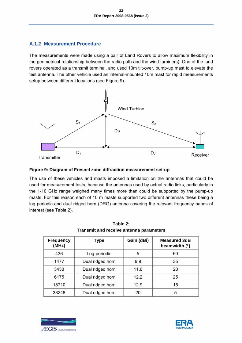
The measurements were made using a pair of Land Rovers to allow maximum flexibility in the geometrical relationship between the radio path and the wind turbine(s). One of the land rovers operated as a transmit terminal, and used 10m tilt-over, pump-up mast to elevate the test antenna. The other vehicle used an internal-mounted 10m mast for rapid measurements setup between different locations (see Figure 9).
Figure 9: Diagram of Fresnel zone diffraction measurement set-up
The use of these vehicles and masts imposed a limitation on the antennas that could be used for measurement tests, because the antennas used by actual radio links, particularly in the 1-10 GHz range weighed many times more than could be supported by the pump-up masts. For this reason each of 10 m masts supported two different antennas these being a log periodic and dual ridged horn (DRG) antenna covering the relevant frequency bands of interest (see Table 2).
Table 2: Transmit and receive antenna parameters
Frequency (MHz)
Type Gain (dBi) Measured 3dB beamwidth (°)
436 Log-periodic 5 60
1477 Dual ridged horn 9.9 35
3430 Dual ridged horn 11.6 20
6175 Dual ridged horn 12.2 25
18710 Dual ridged horn 12.9 15
38248 Dual ridged horn 20 5
Receiver Transmitter
Ds
Wind Turbine
S1 S2
D1 D2

ERA Report 2008-0568 (Issue 3)
34
These types of antennas were used to make fundamental measurements of the power in the direct and reflected paths. The intention of the project was not to assess the overall impact to a particular fixed link system or scanning telemetry device, but to measure and characterise the diffraction/absorption effects from the wind turbine(s).
With the exception of 38248 MHz3, measurements were made at the frequencies shown in Table 2. The transmitter and receiver equipment was mounted in the vehicles, and the antennas fed using standard low-loss coaxial cable (with a low noise amplifier at the receiver masthead). The measured losses are shown in Table 3.
Table 3: Transmit and receive cable losses
Frequency Transmit cable loss (dB) Receive cable loss (dB)
436 1.8 1.7
1477 4.1 3.3
3430 5.4 5.3
6175 7.1 7.2
18710 12.4 12.5
38248 34 32
The transmitter equipment consisted of a synthesised signal generator, a power amplifier of sufficient gain to offset the feeder loss and provide adequate EIRP.
The receiver equipment consisted of a low-noise amplifier mounted at the masthead of the antenna and a spectrum analyser interfaced to a PC for data logging. The Fresnel zone measurements due to diffraction were made by:
• Positioning the transmitter vehicle at a known selected location around the single turbine or wind farm described in Table 1.
• A CW signal at the required frequency was transmitted using a synthesised signal generator via a power amplifier of sufficient gain to offset the feeder loss and provide adequate EIRP.
3 Measurements at 38248 MHz proved difficult to make because the antenna beamwidth was too small to align over relatively large fixed separation distances. Also, the mounts were not stable enough in the strong wind to allow a constant signal level over a separation distance > 1km.

ERA Report 2008-0568 (Issue 3)
35
• For each transmit location the receiver vehicle was positioned at different locations with separation distances of 5 to 10 km relative to the transmitter.
• The latitude and longitude co-ordinate positions of both vehicles were logged automatically using GPS receivers.
• Measurements of the received CW signal were made using a spectrum analyser using a peak detector with a resolution bandwidth (RBW) of 10 kHz and a time span of 10 seconds. This allowed the analyser to record fifty points per second, thus ensuring that any fading of the wanted signal due to the wind turbine(s) was adequately captured.
• Five to ten minutes of measurement data was captured for each frequency at each location to allow meaningful statistical analysis.
The above procedure was repeated for the frequencies shown in Table 2.
A.2 Single Turbine Measurement Results
A.2.1 Measurement Location
Measurement were made around the single Long Hill Road wind turbine in March, Cambridgeshire shown in Figure 10 below.
The transmitter was located at (52.54947° N, 0.03336° E) on the corner to a road leading to Truman Farms off Middle Road. The separation distance to the Long Hill wind turbine from the transmitter was 4.5 km. The receiver was positioned a further 1150 m behind the wind turbine. The transmitter and receiver antennas were aligned such that maximum signal was received i.e., the transmitted and received signal was along bore-sights of each respective antenna with the turbine acting as an obstruction. CW measurements were made at the frequencies shown in Table 2 and the affect from the wind turbine in terms of fading (destructive interference) or enhancements (constructive interference) and any rhythmic patterns observed with the rotation of the wind turbine were recorded.

ERA Report 2008-0568 (Issue 3)
36
Figure 10: Map showing measurement locations along Long Hill Road turbine
A.2.2 Results
Figure 11 and Figure 12 show how the CW signal varied as a function of time with the wind turbine facing the transmitter directly, at frequencies of 436 and 6175 MHz respectively.
At 436 MHz, Figure 11 shows that every 1.2 - 1.3 seconds the turbine produced a null 2 - 2.5 dB below the measured median level.
At 6175 MHz the turbine produced a null of 0.5 – 1.25 dB below the median level, approximately 1.5 dB less than at 436 MHz. This shows that, as the frequency of the transmitted signal increased, the amplitude of the null produced by the wind turbine decreased. This is expected as the Fresnel zone shrinks with increasing frequency (see Eq. 2).

ERA Report 2008-0568 (Issue 3)
37
-64
-63
-62
-61
-60
-59
-58
0 2 4 6 8 10
Time (s)
Rec
eive
d po
wer
(dB
m)
MeasuredMedian
Figure 11: Sample of a measured time trace showing the wind turbine effects to CW at 436 MHz
-79
-78
-77
-76
-75
-74
0 2 4 6 8 10
Time (s)
Rec
eive
d po
wer
(dB
m)
MeasuredMedian
Figure 12: Sample of a measured time trace showing the wind turbine effects to CW at 6175 MHz
During the measurements it was observed that the wind turbine was rotating with an RPM of 15, i.e. every 4 seconds. Thus, with three blades, each tip has an effect on the CW signal every 1.33 seconds. This correlates well with the results shown in the figures above.

ERA Report 2008-0568 (Issue 3)
38
Figure 13 shows the Cumulative Distribution Function (CDF) of the fluctuating signal with respect to its calculated median level, for each measurement frequency. The plot shows that for 1% of the time a single turbine can produce a fade 3 dB below the median signal level at 436 MHz. With the exception of 3430 MHz and 18710 MHz, the level of fade decreases to 2 dB and 1.5 dB for 1477 MHz and 6170 MHz respectively.
Therefore, it can be concluded that a fixed link or scanning telemetry device with a single wind turbine obstructing the direct path between the transmitter and receiver can produce a fade margin ranging between 3 dB to 1.5 dB for 1% of the time.
0
1020
3040
50
6070
8090
100
-4 -3 -2 -1 0 1 2 3 4
Relative signal (dB)
Perc
entil
e (%
) 436 MHz1477 MHz3430 MHz6175 MHz18710 MHz
Figure 13: CDF of the wanted signal relative to its median with increasing frequency for a single turbine
Measurements were also made to try and gauge the extent of the Fresnel zone which had an impact with regards to the fading of the CW signal. The measurements were performed as a function of perpendicular offset distance from the point of the receiver being inline with the wind turbine and transmitter. Figure 14 and Figure 15 below show the results at 436 and 1477 MHz respectively.

ERA Report 2008-0568 (Issue 3)
39
0
1020
3040
50
6070
8090
100
-4 -3 -2 -1 0 1 2 3
Relative signal (dB)
Per
cent
ile (%
)
Inline30 m offset60 m offset
Figure 14: CDF of the wanted 436 MHz signal relative to its median with respect to offset distance from the centre axis
0
1020
3040
50
6070
8090
100
-4 -3 -2 -1 0 1 2 3 4
Relative signal (dB)
Perc
entil
e (%
)
Inline30 m offset60 m offset
Figure 15: CDF of the wanted 1477 MHz signal relative to its median with respect to offset distance from the centre axis
Figure 14 shows that as the receiver system moves off axis from the wind turbine and transmitter, the 1% measured fade below its median decreases from 2.5 dB to 2.2 dB at 30m and 1.2 dB at 60m. This indicates that as the receiver moves away from the centre axis, the level of fading due to the single turbine drops. A similar pattern is also observed when the CW signal is being enhanced.

ERA Report 2008-0568 (Issue 3)
40
A similar trend is observed for a CW signal transmitting at 1477 MHz as shown in Figure 154.
A.3 Wind Farm Measurement Results
A.3.1 Measurement Locations
Measurement were made around the Coldhams wind farm consisting of seventeen turbines in March, Cambridgeshire (see Figure 16). The centre of the wind farm was measured as 52.58371° N, 0.15423° E.
The transmitter was located at (52.542131° N, 0.130215° E) to the entrance of Poplar Farm. The separation distance to the centre of the wind farm from the transmitter was 4.5 km. The receiver was positioned at seven locations as shown in Table 4.
Table 4: Wind farm measurement locations
Position Lat/Long (°N, °E) Land mark Bearing to Tx (°)
Tx and Rx separation
distance (km)
P7 52.61566, 0.17266 Ivy House 207 5.25
P8 52.61306, 0.17324 Needham Farm 200 8.89
P12 52.61809, 0.15934 Maltmas Drove 193 8.3
P13 52.60473, 0.17551 Forties Farm 205 7.5
P14 52.59095, 0.17496 Four Score Farm 213 6.25
P15 52.58666, 0.12445 White House Farm 180 4.95
P16 52.604943, 0.137323 Gate House 185 6.93
4 Due to time constraints measurements could not be made at higher frequencies.

ERA Report 2008-0568 (Issue 3)
41
Figure 16: Map showing measurement locations along Coldhams wind farm
The transmitter and receiver antennas were aligned such that the maximum signal was received, i.e. the transmitted and received signal was along bore-sights of each respective antenna with the wind farm acting as an obstruction. CW measurements were made at the frequencies shown in Table 2 and the affect from the wind turbines in terms of fading (destructive interference) or enhancements (constructive interference) and any rhythmic patterns observed with the rotation of the wind turbine were recorded. During the measurements the wind turbines faced South, South West for the majority of the time.

ERA Report 2008-0568 (Issue 3)
42
A.3.2 Ivy House Results
Figure 17 and Figure 18 show how the CW signal varied as a function of time at P7 (Ivy House) with increasing frequency. The wind turbines were facing South, 30° to the transmitter receiver axis.
-56
-55.5
-55
-54.5
-54
-53.5
-53
0 2 4 6 8 10
Time (s)
Rec
eive
d po
wer
(dB
m)
MeasuredMedian
Figure 17: Sample of a measured time trace at Ivy House showing the wind farm effects to CW at 436 MHz
-71
-70.5
-70
-69.5
-69
-68.5
-68
0 2 4 6 8 10
Time (s)
Rec
eive
d po
wer
(dB
m)
MeasuredMedian
Figure 18: Sample of a measured time trace at Ivy House showing the wind farm effects to CW at 3430 MHz

ERA Report 2008-0568 (Issue 3)
43
The figure below shows the resulting CDF of the fluctuating signal with respect to its calculated median level with increasing frequency.
0
1020
3040
50
6070
8090
100
-5 -3 -1 1 3 5
Relative signal (dB)
Perc
entil
e (%
) 436 MHz1477 MHz3430 MHz6175 MHz18710 MHz
Figure 19: CDF of the wanted signal relative to its median with increasing frequency as measured at Ivy House
The results at 436 MHz show some signs of fast fading and therefore possibly just on the edge of potential interference. At frequencies above 1 GHz the ±1 dB fluctuations in the signal around its median value are due to the local clutter and not from the nearby wind turbines. The perpendicular separation distance measured between the link and the nearest wind turbine was 725 m.
Table 5 shows the comparison between wanted received level based on free space calculations compared with the measured median level at Ivy House. With the exception of 18.71 GHz, the measured results are within 4 to 7 dB with the theoretical values, giving confidence in the results measured.
Table 5: Comparison of calculated and measured received power levels at Ivy House
Frequency (MHz) Free space (dBm) Median level (dBm) Difference (dB)
436 -48.3 -54.6 -6.3
1477 -53.3 -57.3 -4
3430 -66.1 -69.3 -3.2
6175 -48.6 -55.7 -7.1
18710 -95.5 -109.1 -13.6

ERA Report 2008-0568 (Issue 3)
44
A.3.3 Four Score Farm
Moving in an anti-clockwise direction around the wind farm to P14 near Four Score Farm, 1.2 km north of Ivy House, Figure 20 and Figure 21 show how the CW signal varied as a function of time with increasing frequency. At 436 MHz the median signal strength has dropped by 5.8 dB compared with the results at P7.
-65
-64
-63
-62
-61
-60
-59
-58
-57
0 2 4 6 8 10
Time (s)
Rec
eive
d po
wer
(dB
m)
MeasuredMedian
Figure 20: Sample of a measured time trace near Four Score Farm showing the wind farm effects to CW at 436 MHz
-65
-64
-63
-62
-61
-60
-59
-58
-57
0 2 4 6 8 10
Time (s)
Rec
eive
d po
wer
(dB
m)
MeasuredMedian
Figure 21: Sample of a measured time trace near Four Score Farm showing the wind farm effects to CW at 6170 MHz

ERA Report 2008-0568 (Issue 3)
45
The figure below shows the resulting CDF of the fluctuating signal with respect to its calculated median level with increasing frequency.
0
1020
3040
50
6070
8090
100
-6 -4 -2 0 2 4
Relative signal (dB)
Perc
entil
e (%
)
436 MHz1477 MHz3430 MHz6175 MHz
Figure 22: CDF of the wanted signal relative to its median with increasing frequency as measured near Four Score Farm
Figure 20 shows how the CW signal starts to fade more often and with larger drops in signal power compared to it median level. This is due to the wanted signal being blocked and diffracted more as the transmitter receiver path starts to come more into line with the wind turbines. This level of fading drops with respect to increasing frequency as the Fresnel zone reduces according to Eq. 2, (see Figure 21). This assumption can be made because the relative change in the measured median signal level compared with free space calculations is consistent (-8.1 to -10.6 dB) across the frequencies measured.
According to Figure 22, the level of fading of the wanted signal due to a small size wind farm for 1% of the time can be as large as 3 dB at 436 MHz and around 1.5 to 2 dB for frequencies 1.477 GHz and above, for a transmitter receiver link just starting to clip the edge of a outermost wind turbine. These results are similar to the findings for a single turbine as discussed in the previous section.
The perpendicular separation distance measured between the link and the nearest wind turbine was 350 m.
Table 6 shows the comparison between wanted received level based on free space calculations compared with the measured median level at Four Score Farm.

ERA Report 2008-0568 (Issue 3)
46
Table 6: Comparison of calculated and measured received power levels near Four Score Farm
Frequency (MHz) Free space (dBm) Median level (dBm) Difference (dB)
436 -49.8 -60.4 -10.6
1477 -54.8 -66.7 -11.9
3430 -67.6 -79 -11.4
6175 -50.1 -58.2 -8.1
A.3.4 Forties Farm
Moving further north to P13 near Forties Farm, 1.4 km from P14 nearby Four Score Farm, Figure 23 and Figure 24 show how the CW signal varied as a function of time with increasing frequency. At 436 MHz the median level has dropped by a further 6.6 dB compared with the results at P7.
-90
-85
-80
-75
-70
-65
-60
-55
0 2 4 6 8 10
Time (s)
Rec
eive
d po
wer
(dB
m)
MeasuredMedian
Figure 23: Sample of a measured time trace near Forties Farm showing the wind farm effects to CW at 436 MHz
ERA Report 2008-0568 (Issue 3)
47
-63
-62
-61
-60
-59
-58
-57
0 2 4 6 8 10
Time (s)
Rec
eive
d po
wer
(dB
m)
MeasuredMedian
Figure 24: Sample of a measured time trace near Forties Farm showing the wind farm effects to CW at 6175 MHz
The figure below shows the resulting CDF of the fluctuating signal with respect to its calculated median level with increasing frequency.
0
1020
3040
50
6070
8090
100
-25 -20 -15 -10 -5 0 5 10
Relative signal (dB)
Perc
entil
e (%
)
436 MHz1477 MHz3430 MHz6175 MHz
Figure 25: CDF of the wanted signal relative to its median with increasing frequency as measured near Forties Farm

ERA Report 2008-0568 (Issue 3)
48
Figure 23 shows fades as deep as 19 dB relative to the median level were observed when measuring the signal level. These fades are due to the wind turbines causing destructive interference, i.e. the reflected/scattered signal cancelling out the wanted signal when measured at the receiver end.
This level of fading drops with respect to increasing frequency as the Fresnel zone reduces according to Eq. 2, (see Figure 24). With the exception of 3430 MHz measured results, this assumption can be made because the relative change in the measured median signal level compared with free space calculations only changes by 7 to 9 dB from 1477 MHz to 6175 MHz.
The CDF plot in Figure 25 confirms this reduction in fading with respect to increasing frequency. Fades as large as 15 dB at 436 MHz, 10 dB at 1477 MHz and around 2 to 2.5 dB for frequencies 3.43 GHz and above can be detected for 1% of the time, when a transmitter receiver link is being obstructed by a small sized wind farm. The slightly larger fades at 436 MHz are to be expected compared with the other frequency results as the median of the measured wanted signal is the lowest with respect to the free space calculations. The converse is true for the 3430 MHz measured results where the smallest levels of fading are seen; here the median of the wanted signal level is 5 dB higher compared with free space calculations.
Table 7 shows that the median of signal measured at 436 MHz is -15.6 dB below the free space loss calculations thus reducing the received wanted signal enough for the reflected/scattered signal coming off the wind turbines to have a significant affect.
Table 7: Comparison of calculated and measured received power levels near Forties Farm
Frequency (MHz) Free space (dBm) Median level (dBm) Difference (dB)
436 -51.4 -67 -15.6
1477 -56.4 -63.6 -7.2
3430 -69.1 -63.7 5.4
6175 -51 -60.1 -9.1

ERA Report 2008-0568 (Issue 3)
49
A.3.5 Needham Farm
Moving further north to P8 near Needham Farm, 1.4 km from P13 nearby Forties Farm, Figure 26 and Figure 27 show how the CW signal varied as a function of time with increasing frequency. At this location the median level has increased by 3.7 dB at 436 MHz compared with the previous results at P13.
-85
-80
-75
-70
-65
-60
-55
0 2 4 6 8 10
Time (s)
Rec
eive
d po
wer
(dB
m)
MeasuredMedian
Figure 26: Sample of a measured time trace near Needham Farm showing the wind farm effects to CW at 436 MHz
-85
-80
-75
-70
-65
-60
-55
-50
0 2 4 6 8 10
Time (s)
Rec
eive
d po
wer
(dB
m)
MeasuredMedian
Figure 27: Sample of a measured time trace near Needham Farm showing the wind farm effects to CW at 6175 MHz

ERA Report 2008-0568 (Issue 3)
50
The figure below shows the resulting CDF of the fluctuating signal with respect to its calculated median level with increasing frequency.
0
1020
3040
50
6070
8090
100
-25 -20 -15 -10 -5 0 5 10
Relative signal (dB)
Perc
entil
e (%
)
436 MHz1477 MHz3430 MHz6175 MHz
Figure 28: CDF of the wanted signal relative to its median with increasing frequency as measured near Needham Farm
Figure 26 shows fades as deep as 16 dB relative to the median level were observed when measuring the signal level. These fades are due to the wind turbines causing destructive interference, i.e. the reflected/scattered signal cancelling out the wanted signal when measured at the receiver end. It is also interesting to note that the level of fade reduced by the same amount as the median of the wanted signal from measurement point P13 to measurement point P8.
Figure 27 shows that the level of fading seen at the receiver does not reduce like previous measurements points.
The CDF plot in Figure 28 confirms this constant fading with respect to increasing frequency. Fades as large as 10 dB at 436 MHz, 7 dB at 1477 MHz, 12 dB at 3430 MHz and 9 dB at 6175 MHz can be detected for 1% of the time, when a transmitter receiver link is being completely obstructed by a small sized wind farm. The slightly larger fades at 436 MHz are to be expected compared with the other frequency results as the median of the measured wanted signal is the lowest with respect to the free space calculations. The converse is true for the 3430 MHz measured results where the smallest levels of fading are seen; here the median of the wanted signal level is 5 dB higher compared with free space calculations.

ERA Report 2008-0568 (Issue 3)
51
The fades are to be expected as the wind farm is blocking the direct link between the transmitter and receiver, hence reducing the wanted signal. With the exception of 3430 MHz, Table 8 shows that the median of the signal measured for all frequencies is 10 dB or more below the free space loss calculations. Therefore, the signal reflected/scattered from the wind turbines will have a significant destructive affect.
Table 8: Comparison of calculated and measured received power levels near Needham Farm
Frequency (MHz) Free space (dBm) Median level (dBm) Difference (dB)
436 -52.9 -63.3 -10.4
1477 -57.9 -72 -14.1
3430 -40.7 -48.4 -7.7
6175 -53.2 -66.7 -13.5
A.3.6 Maltmas Drove
Moving further east to P12 at Maltmas Drove, 1.4 km from P8 nearby Needham Farm, Figure 29 and Figure 30 show how the CW signal varied as a function of time with increasing frequency.
-95
-90
-85
-80
-75
-70
-65
-60
0 2 4 6 8 10
Time (s)
Rec
eive
d po
wer
(dB
m)
MeasuredMedian
Figure 29: Sample of a measured time trace at Maltmas Drove showing the wind farm effects to CW at 1477 MHz

ERA Report 2008-0568 (Issue 3)
52
-80
-75
-70
-65
-60
-55
0 2 4 6 8 10
Time (s)
Rec
eive
d po
wer
(dB
m)
MeasuredMedian
Figure 30: Sample of a measured time trace at Maltmas Drove showing the wind farm effects to CW at 6175 MHz
The figure below shows the resulting CDF of the fluctuating signal with respect to its calculated median level with increasing frequency.
0
1020
3040
50
6070
8090
100
-20 -15 -10 -5 0 5 10
Relative signal (dB)
Per
cent
ile (%
)
436 MHz1477 MHz3430 MHz6175 MHz
Figure 31: CDF of the wanted signal relative to its median with increasing frequency as measured at Maltmas Drove

ERA Report 2008-0568 (Issue 3)
53
Figure 29 shows that fades as deep as 21 dB relative to the median level were observed when measuring the signal level. These fades are again due to the wind turbines causing destructive interference, i.e., the reflected/scattered signal cancelling out the wanted signal when measured at the receiver end.
Figure 30 show that the level of fading drops with increasing frequency, by as much as 10 dB.
The CDF plot in Figure 31 show that fades as large as 7 dB at 436 MHz, 12 dB at 1477 MHz, 6 dB at 3430 MHz and above can be detected for 1% of the time, when a transmitter receiver link is being completely obstructed by a small sized wind farm.
The fades are to be expected as the wind farm is blocking the direct link between the transmitter and receiver, hence reducing the wanted signal. With the exception of 3430 MHz measurement result, Table 9 shows that the median of the signal measured for all frequencies is 11 to 14 dB below the free space loss calculations. Therefore, the signal reflected/scattered from the wind turbines will have a significant destructive affect.
Table 9: Comparison of calculated and measured received power levels at Maltmas Drove
Frequency (MHz) Free space (dBm) Median level (dBm) Difference (dB)
436 -52.3 -63.7 -11.4
1477 -57.3 -70.1 -12.8
3430 -40 -42.8 -2.8
6175 -52.3 -66.4 -14.1
Once again, with the exception of the 436 MHz results, measurements at P12 show the level of fading drops with respect to increasing frequency. The results at 436 MHz prove to be inconsistent with previous measurement points. This may me due to the fact that only half the wind turbines were rotating compared with the 1477 MHz measured results.

ERA Report 2008-0568 (Issue 3)
54
A.3.7 Gate House
Moving to P16 at Gate House, 1.1 km south of P12 at Maltmas Drove, Figure 32 and Figure 33 show how the CW signal varied as a function of time with increasing frequency.
-68
-67
-66
-65
-64
-63
-62
-61
-60
0 2 4 6 8 10
Time (s)
Rec
eive
d po
wer
(dB
m)
MeasuredMedian
Figure 32: Sample of a measured time trace at Gate House showing the wind farm effects to CW at 436 MHz
-68
-67
-66
-65
-64
-63
-62
-61
-60
0 2 4 6 8 10
Time (s)
Rec
eive
d po
wer
(dB
m)
MeasuredMedian
Figure 33: Sample of a measured time trace at Gate House showing the wind farm effects to CW at 6175 MHz

ERA Report 2008-0568 (Issue 3)
55
The figure below shows the resulting CDF of the fluctuating signal with respect to its calculated median level with increasing frequency.
0
1020
3040
50
6070
8090
100
-6 -4 -2 0 2 4
Relative signal (dB)
Perc
entil
e (%
)
436 MHz1477 MHz3430 MHz6175 MHz
Figure 34: CDF of the wanted signal relative to its median with increasing frequency as measured at Gate House
Figure 32 shows that fades as deep as 4 dB relative to the median level were observed when measuring the signal level. These fades are again due to the wind turbines causing destructive interference, i.e. the reflected/scattered signal cancelling out the wanted signal when measured at the receiver end.
The perpendicular separation distance measured between the link and the nearest wind turbine in this scenario was 625 m.
Figure 33 shows a cleaner trace compared with the 436 MHz results, probably due to the clutter and surrounding environment having more of a dominant affect compared with the diffraction of the wanted signal due to the wind turbines.
The CDF plot in Figure 34 shows that fades as large as 3 dB at 436 MHz, 1.5 dB at 1477 MHz, 2.5 dB at 3430 MHz and above can be detected for 1% of the time, when a transmitter receiver link is partially obstructed by a small sized wind farm. These results are similar to the findings for a single turbine as discussed in the previous section.
The fades shown in the plots are to be expected as the wind farm is partially blocking the direct link between the transmitter and receiver, hence reducing the wanted signal. With the exception of 3430 MHz, Table 10 shows that the median of the signal measured for all

ERA Report 2008-0568 (Issue 3)
56
frequencies is 11 to 14 dB below the free space loss calculations. Therefore, the signal reflected/scattered from the wind turbines will have a significant destructive affect.
Table 10: Comparison of calculated and measured received power levels at Gate House
Frequency (MHz) Free space (dBm) Median level (dBm) Difference (dB)
436 -50.7 -63.6 -12.9
1477 -55.7 -66.7 -11
3430 -38.5 -42.8 -4.3
6175 -51.7 -65.3 -13.6
Once again, the measurements at P16 show the level of fading drops with respect to increasing frequency. The 1477 MHz results produced a very clean recorded signal showing no signs of interference from the wind farm and surrounding clutter. However, the results at higher frequencies point to clutter being more dominant in the fading of the wanted signal. This can be identified by the slow nature of the fades compared with that seen from the wind turbines.
A.3.8 White House Farm
Moving near to White House Farm (P15), 2 km south of Gate House (P16), Figure 35 and Figure 36 show how the CW signal varied as a function of time with increasing frequency
-55-54.8-54.6-54.4-54.2
-54-53.8-53.6-53.4-53.2
-53
0 2 4 6 8 10
Time (s)
Rec
eive
d po
wer
(dB
m)
MeasuredMedian
Figure 35: Sample of a measured time trace near White House Farm showing the wind farm effects to CW at 436 MHz

ERA Report 2008-0568 (Issue 3)
57
-67
-66
-65
-64
-63
-62
-61
-60
0 2 4 6 8 10
Time (s)
Rec
eive
d po
wer
(dB
m)
MeasuredMedian
Figure 36: Sample of a measured time trace near White House Farm showing the wind farm effects to CW at 6175 MHz
The figure below shows the resulting CDF of the fluctuating signal with respect to its calculated median level with increasing frequency.
0
1020
3040
50
6070
8090
100
-6 -4 -2 0 2 4
Relative signal (dB)
Perc
entil
e (%
)
436 MHz1477 MHz3430 MHz6175 MHz
Figure 37: CDF of the wanted signal relative to its median with increasing frequency as measured near White House Farm

ERA Report 2008-0568 (Issue 3)
58
The drop in signal level shown in Figure 35 can be explained by the larger numbers of trees between the transmitter and receiver line-of-sight. Also, the plot reveals no significant fades resulting from the wind turbines affect the wanted signal at 436 MHz. This was observed for all higher measured frequencies. However, for measurements made at 3430 MHz and 6175 MHz the surrounding foliage and trees had an impact on the recorded signal as shown in Figure 36.
The CDF plot in Figure 37 shows that fades as large as 0.4 dB at 436 MHz, 0.7 dB at 1477 MHz, 3.2 dB at 3430 MHz and 3.9 dB at 6175 MHz can be detected for 1% of the time. These results are due the local clutter and not from the nearby wind turbines.
Table 11 shows the comparison between wanted received level based on free space calculations compared with the measured median level near White House Farm for frequencies from 436 MHz and 6.175 GHz. The table shows that the measured results vary from 6 to 15 dB with the theoretical values. This 9 dB difference can be explained by the local clutter affecting the received wanted signal.
Table 11: Comparison of calculated and measured received power levels near White House
Farm
Frequency (MHz) Free space (dBm) Median level (dBm) Difference (dB)
436 -47.8 -53.8 -6
1477 -52.8 -65 -12.2
3430 -35.6 -42.2 -6.6
6175 -48.1 -63.1 -15
A.4 Near-field Analysis
Near-field measurements to examine the degree of interaction between a terminal antenna and a turbine were not performed. For large-aperture antennas operating at higher frequencies, the near-field zone can extend to several kilometres. For the antennas which could be accommodated on the measurement vehicles, the near-field distances were calculated to be very small, as illustrated in Table 12. Therefore, it seemed unnecessary to address this phenomenon by direct measurement.
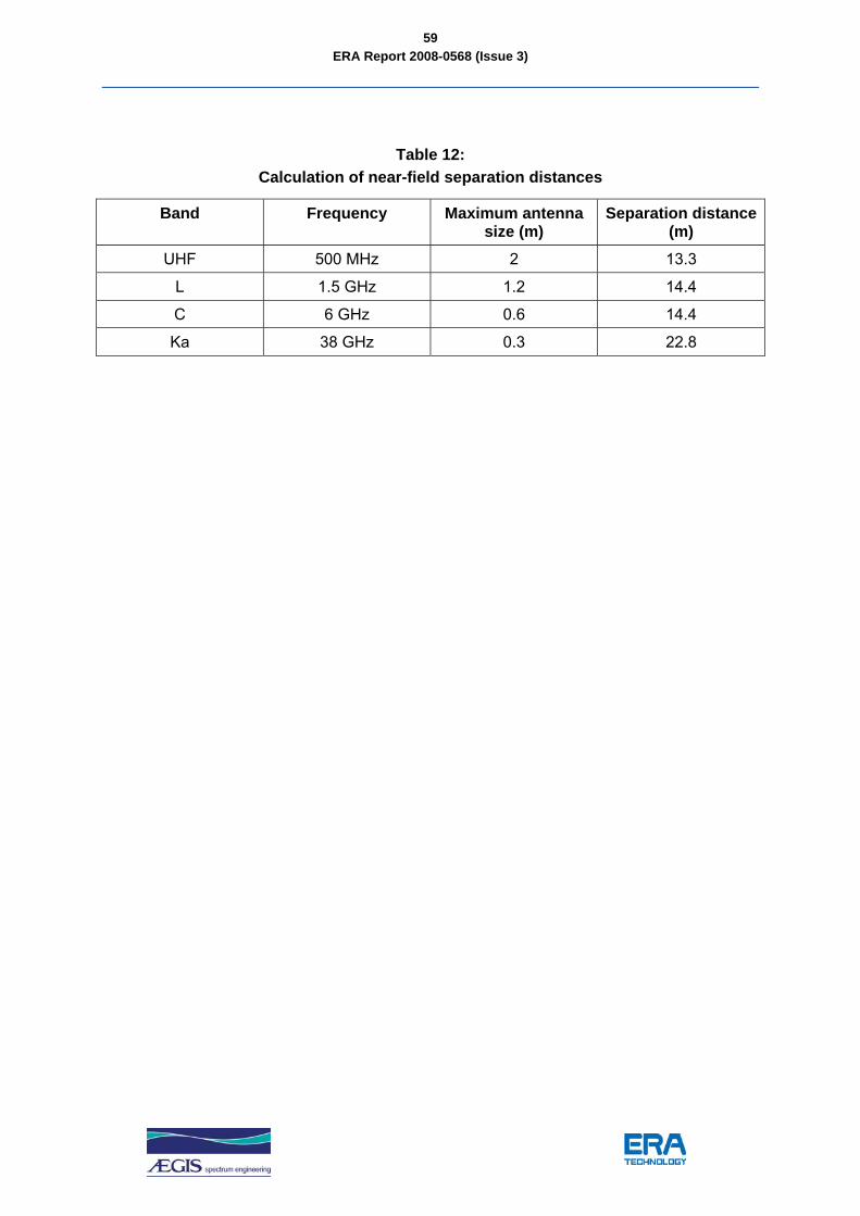
ERA Report 2008-0568 (Issue 3)
59
Table 12: Calculation of near-field separation distances
Band Frequency Maximum antenna size (m)
Separation distance (m)
UHF 500 MHz 2 13.3
L 1.5 GHz 1.2 14.4
C 6 GHz 0.6 14.4
Ka 38 GHz 0.3 22.8

ERA Report 2008-0568 (Issue 3)
60
This page is intentionally left blank

ERA Report 2008-0568 (Issue 3)
61
APPENDIX B Aegis Measurements
ERA Report 2008-0568 (Issue 3)
62
B.1 Test Methodology
The main difficulty in making measurements of scatter from discrete objects in the landscape lies in separating the contributions to the scattered field from different sources. For most relative geometries, however, the relative delay of the scattered or reflected energy will be different for each object. If measurements are made in the time domain (as in a radar system), the various contributions may be examined individually.
In each case, one or more transmitter sites were chosen, and the initial measurement made was of the backscatter case, with the receiver van parked adjacent to the transmitter, and with both aerials pointing at the wind turbine, or the centre of the wind farm. Further measurements were then made for the bi-static scattering case, with the receiver van moved to locations well separated from the transmitter.
The intention of the measurements was to determine the power scattered from individual turbines for each geometry. The use of a channel sounder allowed the scattering due to individual turbines to be quantified for each geometry.
B.1.1 Measurement approach
Aegis systems have developed a wideband channel sounder, originally for use in an unrelated research project for Ofcom. The sounder uses a 511-bit pseudo-noise (PN) sequence clocked at 10 MHz to modulate a carrier at one of three test frequencies (436 MHz, 1477 MHz and 3430 MHz).
The receiver uses a direct conversion architecture to recover I and Q baseband channels, which are captured by an ADC, sampling at 50 Msamples/s. As the oscillators in both terminals are locked to rubidium oscillators, phase stability is sufficient to recover the complex channel information.
In off-line processing, the received PN sequence spectrum is convolved with that of the transmitted sequence, and the power delay profile of the channel recovered using the Wiener-Kinchin relationship.
The results of a typical sounder measurement are shown in Figure 38, with sample time on the axis towards the reader, and excess delay increasing from left to right. The direct, line of sight, signal is represented by the peak at the left of the plot, and a number of discrete, permanent reflections are evident, two of which are indicated by the red arrowed lines.
Some of these reflections will correspond to individual wind turbines, while others will be due to other clutter, such as pylons.
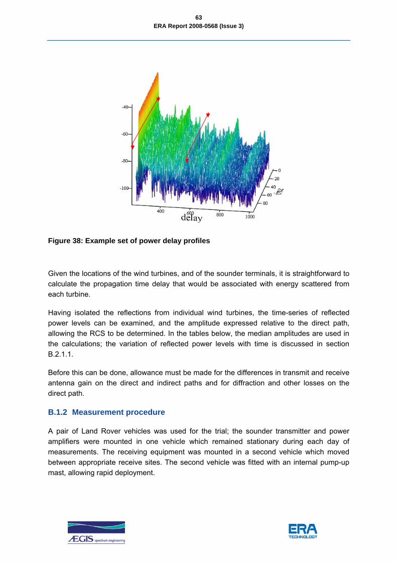
ERA Report 2008-0568 (Issue 3)
63
Figure 38: Example set of power delay profiles
Given the locations of the wind turbines, and of the sounder terminals, it is straightforward to calculate the propagation time delay that would be associated with energy scattered from each turbine.
Having isolated the reflections from individual wind turbines, the time-series of reflected power levels can be examined, and the amplitude expressed relative to the direct path, allowing the RCS to be determined. In the tables below, the median amplitudes are used in the calculations; the variation of reflected power levels with time is discussed in section B.2.1.1.
Before this can be done, allowance must be made for the differences in transmit and receive antenna gain on the direct and indirect paths and for diffraction and other losses on the direct path.
B.1.2 Measurement procedure
A pair of Land Rover vehicles was used for the trial; the sounder transmitter and power amplifiers were mounted in one vehicle which remained stationary during each day of measurements. The receiving equipment was mounted in a second vehicle which moved between appropriate receive sites. The second vehicle was fitted with an internal pump-up mast, allowing rapid deployment.
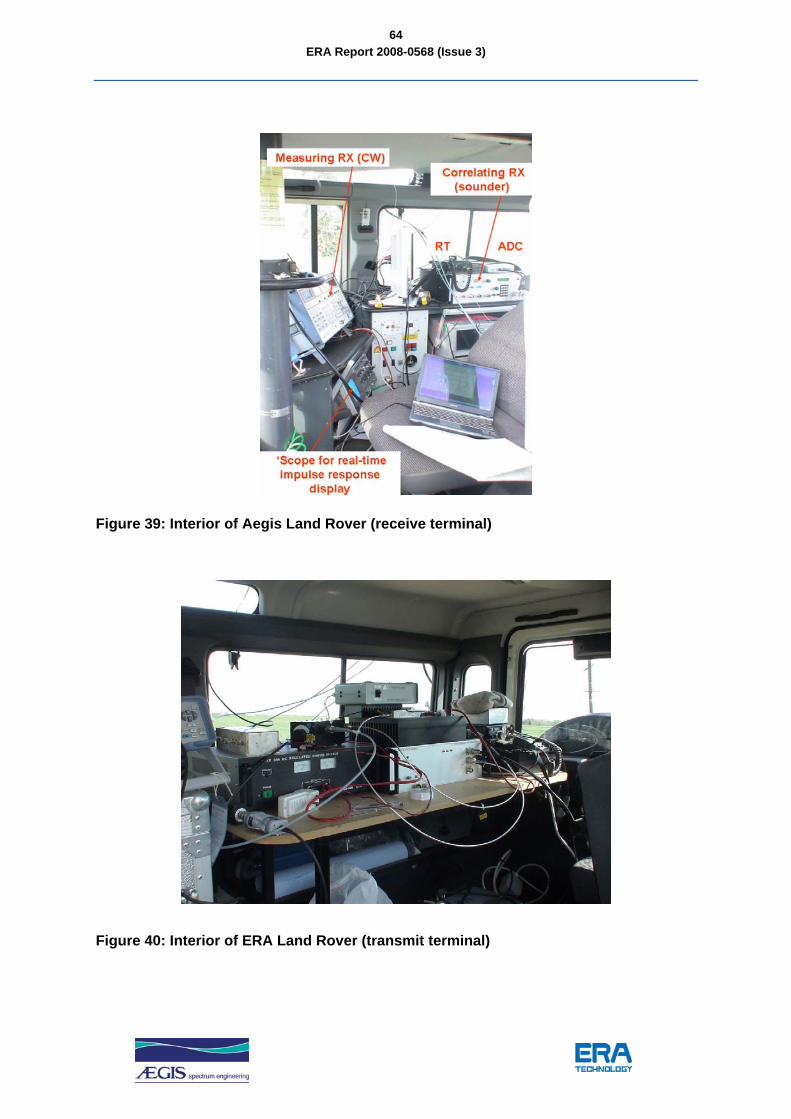
ERA Report 2008-0568 (Issue 3)
64
Figure 39: Interior of Aegis Land Rover (receive terminal)
Figure 40: Interior of ERA Land Rover (transmit terminal)

ERA Report 2008-0568 (Issue 3)
65
Both terminals used the same antennas, mounted at a nominal height of 10 m above ground. Details are given in the table below.
Table 13: Measurement system characteristics
Frequency (MHz)
Bandwidth (MHz)
Tx EIRP (dBW)
Feeder loss (dB) (Tx/Rx)
Aerial type Aerial gain (dBi) (Tx and Rx)
436 5 20 1.8 / 1.7 Log-periodic 5
1477 20 20 4.1 / 3.3 Horn 9.9
3420 20 20 5.4 / 5.3 Horn 11.6
The horizontal radiation patterns (HRP) of the antennas used have been measured by ERA, and are shown in the Figures below.
-18-16-14-12-10-8-6-4-202
180185 190 195200
205210
215220
225230
235240
245
250
255
260
265
270
275
280
285
290
295300
305310
315320
325330
335340345350355
05101520
2530
3540
4550
5560
65
70
75
80
85
90
95
100
105
110
115120
125130
135140
145150
155160165 170 175
Figure 41: 436 MHz antenna HRP

ERA Report 2008-0568 (Issue 3)
66
-40
-30
-20
-10
0180
185 190 195 200205
210215
220225
230
235
240
245
250
255
260
265
270
275
280
285
290
295
300
305
310315
320325
330335
3403453503550
510152025
3035
4045
50
55
60
65
70
75
80
85
90
95
100
105
110
115
120
125
130135
140145
150155
160 165 170 175
Figure 42: 1477 MHz antenna HRP
-25
-20
-15
-10
-5
0180
185 190 195 200205
210215
220225
230
235
240
245
250
255
260
265
270
275
280
285
290
295
300
305
310315
320325
330335
3403453503550
510152025
3035
4045
50
55
60
65
70
75
80
85
90
95
100
105
110
115
120
125
130135
140145
150155
160 165 170 175
Figure 43: 3430 MHz antenna pattern
These measured patterns have been used to correct for the differences in overall system gain on the direct transmitter-receiver path, and on the indirect paths via the individual turbines.

ERA Report 2008-0568 (Issue 3)
67
B.2 Single Turbine Measurement Results
Initial measurements were made of single wind turbine, located at Long Hill Road, near a prison and railway marshalling yards.
B.2.1 Grandford transmit site
The first series of measurements were made with the transmitter near Grandford House, some 2.5 km to the west of the turbine, and with the receiver van placed to examine backscatter, forward scatter and intermediate geometries, as shown in Figure 44.
Figure 44: Single Turbine – Grandford transmit site
Although the single turbine is a relatively prominent feature, it was found to be rather difficult to distinguish (in radio terms) from local clutter – in particular a series of pylons (seen in Figure 45) runs close to the turbine, and strong reflections were also noted from nearby metal buildings and a radio mast.

ERA Report 2008-0568 (Issue 3)
68
Figure 45: Single Turbine seen from Grandford transmit site (TX on left)
Traffic on the road (A141) between the terminals and the wind turbine also produced large reflections, as can be seen from the plot of Figure 46.
Figure 46: Power delay profiles measured at Grandford, showing intermittent return from traffic

ERA Report 2008-0568 (Issue 3)
69
B.2.1.1 Backscatter
The turbine at Long Hill Road is at 2.65 km from the site at Grandford, and the delay for the backscatter case is therefore 17.6 μS. The power delay profile record was examined at this delay, and the time-series of received power extracted.
The close proximity of the transmitter van precludes a direct measurement of the relative amplitude of direct and reflected waves (the direct path is only ~10 m, and relative antenna gains are uncertain). Given the sounder system link budget, values for the RCS may be determined from this data, and the results are shown in Figure 47 for 1477 MHz. This plot shows the variation in RCS with time. During the measurements, the turbine was pointing south west, so that it was presenting a fairly small aspect to the Grandford site. The pitch of the blades was unknown.
Long Hill Road Backscatter
2526
2728
293031
3233
3435
0 5 10 15 20 25 30 35 40
Time (seconds)
RC
S (d
Bm
^2)
Figure 47: Backscatter RCS at 1477 MHz
The recovered RCS data is somewhat under sampled (constrained by the current logging software and ADC in the sounder). The turbine was rotating with a period of around 4 seconds, and the data appears to reflect the expected periodicity for a 3-bladed turbine.
B.2.1.2 Side scatter (Stag’s Holt receiver)
At the Stag’s Holt receiver site, the sounding system has a bistatic angle of around 140°. Under these conditions a lower RCS would be expected than for the backscatter (or forward scatter) cases.
The determination of the RCS is somewhat simpler (and more accurate) for the bistatic case (tx and rx at separate locations), as the difference between the direct and reflected signals can be examined directly.
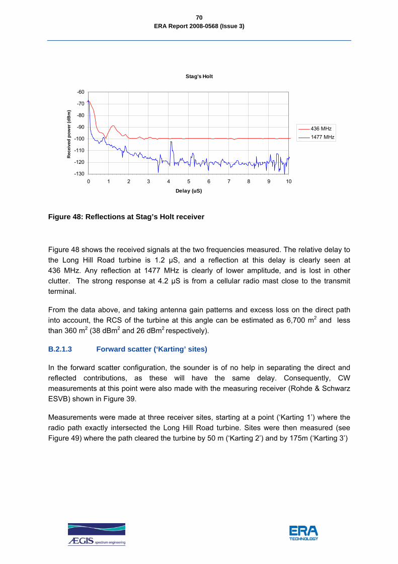
ERA Report 2008-0568 (Issue 3)
70
Stag's Holt
-130
-120
-110
-100
-90
-80
-70
-60
0 1 2 3 4 5 6 7 8 9 10
Delay (uS)
Rec
eive
d po
wer
(dB
m)
436 MHz1477 MHz
Figure 48: Reflections at Stag’s Holt receiver
Figure 48 shows the received signals at the two frequencies measured. The relative delay to the Long Hill Road turbine is 1.2 μS, and a reflection at this delay is clearly seen at 436 MHz. Any reflection at 1477 MHz is clearly of lower amplitude, and is lost in other clutter. The strong response at 4.2 μS is from a cellular radio mast close to the transmit terminal.
From the data above, and taking antenna gain patterns and excess loss on the direct path into account, the RCS of the turbine at this angle can be estimated as 6,700 m2 and less than 360 m2 (38 dBm2 and 26 dBm2 respectively).
B.2.1.3 Forward scatter (‘Karting’ sites)
In the forward scatter configuration, the sounder is of no help in separating the direct and reflected contributions, as these will have the same delay. Consequently, CW measurements at this point were also made with the measuring receiver (Rohde & Schwarz ESVB) shown in Figure 39.
Measurements were made at three receiver sites, starting at a point (‘Karting 1’) where the radio path exactly intersected the Long Hill Road turbine. Sites were then measured (see Figure 49) where the path cleared the turbine by 50 m (‘Karting 2’) and by 175m (‘Karting 3’)

ERA Report 2008-0568 (Issue 3)
71
Figure 49: Near forward scatter paths at ‘Karting’ site
Comparison of the median received level with the predicted free space value indicates that there is some 11 dB (436 MHz) and 4 dB (1477 MHz) of loss on the direct path, largely due to the inadequate path clearance owing to the low terminal antenna heights used, as shown by the Fresnel zone dimensions indicated in Figure 50 and Figure 51.
Figure 50: Path geometry at 436 MHz

ERA Report 2008-0568 (Issue 3)
72
Figure 51: Path geometry at 1477 MHz
From the plots of CW received power below, it can be seen that the impact of the turbine on the received power diminishes quite rapidly as the radio path moves away from the obstruction.
Figure 52 shows the fully obstructed case, showing a very clear and regular pattern of interference at the lower frequency. At the time of the measurement, the turbine period was around 6 seconds which, with three blades, implies that a symmetry should be observed with a two second period, which is the case. Interference effects are less at the higher frequency not because the turbine is less reflective, but largely because the wanted path excess loss is lower at this frequency.
An important point to note is that the impact of the turbine does not appear to be an occultation of the path, but rather a periodic enhancement of some 2-3 dB. This implies that a forward scattered wave is adding constructively to the direct wave as each blade in turn comes into a critical relative position. For coherent interference, a 3 dB enhancement would imply that the amplitude of the reflected wave is some 8 dB below the direct wave. Given the attenuation of the direct wave noted above, the C/I ratio for a properly-engineered link with full Fresnel zone clearance would be in the order of 20 dB. This would correspond to a forward scatter RCS of 200,000 m2 (53 dBm2); though dramatically in excess of the physical projection of the turbine, this value is almost the same as that calculated in Section 2.5.2.
Figure 53 shows the interference experienced with a 50 m horizontal clearance of the turbine, which is sufficient to place the blades beyond the first Fresnel zone in both cases. There is now less than 1 dB of peak-peak variation at 1477 MHz, while some 2 dB of variability is evident at the lower frequency. It should be noted that, whereas the effect in the in-line case was one of enhancement to the median value, for this geometry interference

ERA Report 2008-0568 (Issue 3)
73
nulls are recorded. This emphasises that the interference mechanism is one of interference between direct and reflected waves, rather than of attenuation by absorption or blocking.
Karting 1
73
74
75
76
7778
79
80
81
82
83
0 10 20 30 40 50 60
seconds
dBuV 1477 MHz
436 MHz
Figure 52: CW measurements with path through turbine
Karting 2
65
66
67
68
6970
71
72
73
74
75
0 10 20 30 40 50 60
seconds
dBuV 1477 MHz
436 MHz
Figure 53: CW measurements with 50m path clearance

ERA Report 2008-0568 (Issue 3)
74
Karting 3
65
66
67
68
6970
71
72
73
74
75
0 10 20 30 40 50 60
seconds
dBuV 1477 MHz
436 MHz
Figure 54: CW measurements with 175m path clearance
In the final plot, Figure 54, with 175 m lateral clearance, no variation attributable to the wind farm can be seen at the higher frequency, while at 436 MHz, the effect is less than 1 dB peak-peak. Bearing in mind that the direct path suffers some 11 dB loss, no effect would be noted on a properly engineered link.
While the sounder cannot resolve the reflected and direct contributions, as there is minimal path difference, it is instructive to examine the received spectrum of the sounding signal. The plots of received CW power show significant coherent additions or nulls due to interference, but the impact of these effects will be less on the overall power of a wideband signal.
Some frequency selective fading of the sounding signal can be seen in Figure 55, though the fading is generally flat over the sounder bandwidth (as must be the case if the components cannot be separated in the time domain).
Figure 55: Showing frequency selective fading (1477 MHz)
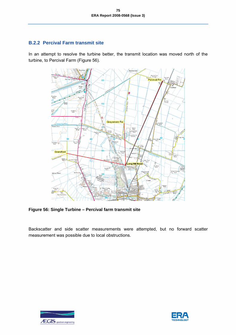
ERA Report 2008-0568 (Issue 3)
75
B.2.2 Percival Farm transmit site
In an attempt to resolve the turbine better, the transmit location was moved north of the turbine, to Percival Farm (Figure 56).
Figure 56: Single Turbine – Percival farm transmit site
Backscatter and side scatter measurements were attempted, but no forward scatter measurement was possible due to local obstructions.

ERA Report 2008-0568 (Issue 3)
76
Figure 57: Single Turbine seen from Graysmore farm receive site
The Graysmore receive location had a direct line-of-sight to the turbine, which was clearly visible5 on the sounder response (see Figure 58).
5 The 436 MHz measurement has an artificially high noise floor owing to an incorrect attenuator setting being used

ERA Report 2008-0568 (Issue 3)
77
Percival Fm - LHR - Graysmore 1477 MHz
-120
-110
-100
-90
-80
-70
-60
-50
-40
-30
0 2 4 6 8 10 12 14
Delay (uS)
Mea
sure
men
t (dB
)
1477 MHz436 MHzturbine
Figure 58: Sounder response at Graysmore receive site
It can be seen that at neither frequency does the turbine stand out particularly strongly from the clutter.
When corrections are made for the directionality of the transmit and receive antennas, the RCS of the turbine was found to be 400 m2 (436 MHz) and 50m2 (1477 MHz) or 26 dBm2 and 17 dBm2 respectively. These values are subject to an uncertainty of some +/- 6 dB owing to the lack of precision with which antenna gains can be determined for this particular geometry (the transmitter is ~135° off-bore-sight at the receiver).
B.2.3 Summary
The results obtained are summarised in the table below.
Table 14: Summary results for single turbine measurements
RCS (dBm²) Frequency (MHz)
Backscatter Intermediate Forward scatter
436 47 26 - 38 53
1477 32 17 - 26 50

ERA Report 2008-0568 (Issue 3)
78
B.3 Wind Farm Measurement Results
Following the measurements of the single turbine at Long Hill Road, the trials moved to the nearby wind farm sites of Stag’s Holt and Coldham.
Figure 59: Measurements of Coldham / Stag’s Holt wind farm (Poplar Fm Tx)
As before, measurements were made for the backscatter, forward scatter and intermediate cases, though time allowed only one transmit site to be used.
The turbines on the wind farm site were very much more ‘visible’ to the sounder than was the case for the Long Hill Road turbine, which was somewhat lost in the clutter. Examples of the sounder response at each frequency are shown in Figure 60, on which the predicted delays to each of the 17 turbines are also shown.
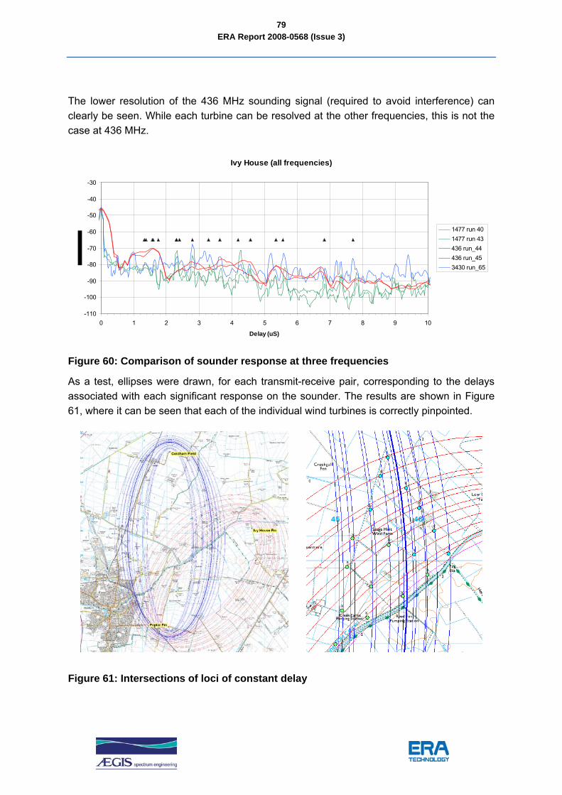
ERA Report 2008-0568 (Issue 3)
79
The lower resolution of the 436 MHz sounding signal (required to avoid interference) can clearly be seen. While each turbine can be resolved at the other frequencies, this is not the case at 436 MHz.
Ivy House (all frequencies)
-110
-100
-90
-80
-70
-60
-50
-40
-30
0 1 2 3 4 5 6 7 8 9 10
Delay (uS)
1477 run 40 1477 run 43436 run_44436 run_453430 run_65
Figure 60: Comparison of sounder response at three frequencies
As a test, ellipses were drawn, for each transmit-receive pair, corresponding to the delays associated with each significant response on the sounder. The results are shown in Figure 61, where it can be seen that each of the individual wind turbines is correctly pinpointed.
Figure 61: Intersections of loci of constant delay
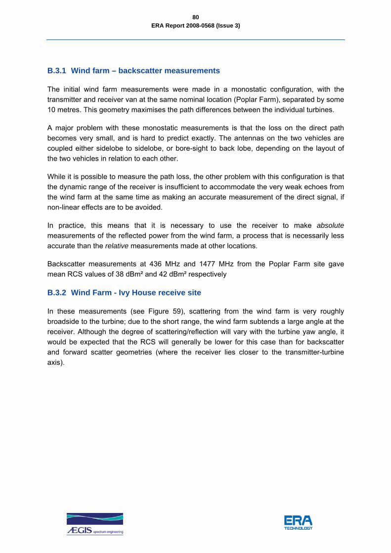
ERA Report 2008-0568 (Issue 3)
80
B.3.1 Wind farm – backscatter measurements
The initial wind farm measurements were made in a monostatic configuration, with the transmitter and receiver van at the same nominal location (Poplar Farm), separated by some 10 metres. This geometry maximises the path differences between the individual turbines.
A major problem with these monostatic measurements is that the loss on the direct path becomes very small, and is hard to predict exactly. The antennas on the two vehicles are coupled either sidelobe to sidelobe, or bore-sight to back lobe, depending on the layout of the two vehicles in relation to each other.
While it is possible to measure the path loss, the other problem with this configuration is that the dynamic range of the receiver is insufficient to accommodate the very weak echoes from the wind farm at the same time as making an accurate measurement of the direct signal, if non-linear effects are to be avoided.
In practice, this means that it is necessary to use the receiver to make absolute measurements of the reflected power from the wind farm, a process that is necessarily less accurate than the relative measurements made at other locations.
Backscatter measurements at 436 MHz and 1477 MHz from the Poplar Farm site gave mean RCS values of 38 dBm² and 42 dBm² respectively
B.3.2 Wind Farm - Ivy House receive site
In these measurements (see Figure 59), scattering from the wind farm is very roughly broadside to the turbine; due to the short range, the wind farm subtends a large angle at the receiver. Although the degree of scattering/reflection will vary with the turbine yaw angle, it would be expected that the RCS will generally be lower for this case than for backscatter and forward scatter geometries (where the receiver lies closer to the transmitter-turbine axis).

ERA Report 2008-0568 (Issue 3)
81
Figure 62: Ivy House Site looking North West
The direct path from transmitter to receiver is 5.27 km, and the loss on this path has been estimated for each frequency. It is assumed that all turbines are line-of-sight to both terminals, and that there is, therefore, no loss beyond free-space on the reflected paths.
The transmitter and receiver antennas were directed at the wind farm (nominally towards turbine C2). The transmitter antenna bore-sight was, therefore 23.7° away from the direction of the receiver site, and the receive antenna bore-sight 75.6° from the direction of the transmitter site (see Figure 59).
B.3.2.1 436 MHz
At this location, there is 4.5 dB of combined antenna discrimination on the direct path. Smooth earth diffraction loss6 is calculated at 10 dB, with an estimated 2 dB of additional loss from vegetation and clutter.
6 Including 2-ray interference
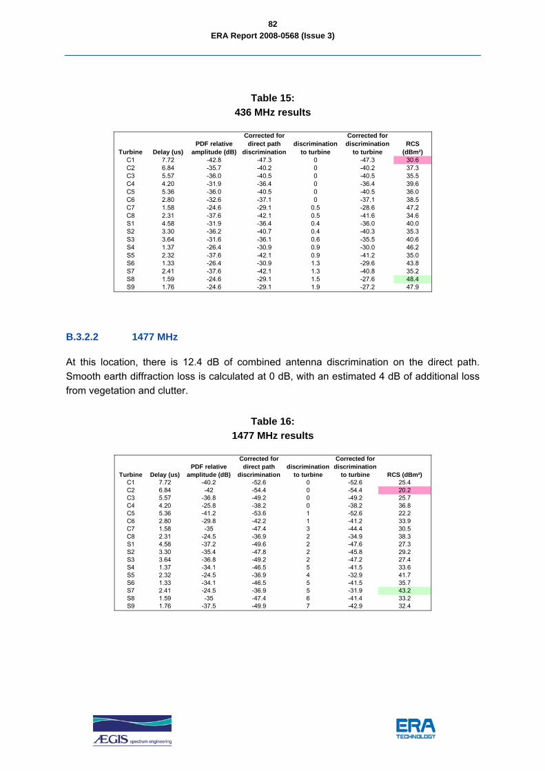
ERA Report 2008-0568 (Issue 3)
82
Table 15: 436 MHz results
Turbine Delay (us)PDF relative
amplitude (dB)
Corrected for direct path
discriminationdiscrimination
to turbine
Corrected for discrimination
to turbineRCS
(dBm²)C1 7.72 -42.8 -47.3 0 -47.3 30.6C2 6.84 -35.7 -40.2 0 -40.2 37.3C3 5.57 -36.0 -40.5 0 -40.5 35.5C4 4.20 -31.9 -36.4 0 -36.4 39.6C5 5.36 -36.0 -40.5 0 -40.5 36.0C6 2.80 -32.6 -37.1 0 -37.1 38.5C7 1.58 -24.6 -29.1 0.5 -28.6 47.2C8 2.31 -37.6 -42.1 0.5 -41.6 34.6S1 4.58 -31.9 -36.4 0.4 -36.0 40.0S2 3.30 -36.2 -40.7 0.4 -40.3 35.3S3 3.64 -31.6 -36.1 0.6 -35.5 40.6S4 1.37 -26.4 -30.9 0.9 -30.0 46.2S5 2.32 -37.6 -42.1 0.9 -41.2 35.0S6 1.33 -26.4 -30.9 1.3 -29.6 43.8S7 2.41 -37.6 -42.1 1.3 -40.8 35.2S8 1.59 -24.6 -29.1 1.5 -27.6 48.4S9 1.76 -24.6 -29.1 1.9 -27.2 47.9
B.3.2.2 1477 MHz
At this location, there is 12.4 dB of combined antenna discrimination on the direct path. Smooth earth diffraction loss is calculated at 0 dB, with an estimated 4 dB of additional loss from vegetation and clutter.
Table 16: 1477 MHz results
Turbine Delay (us)PDF relative
amplitude (dB)
Corrected for direct path
discriminationdiscrimination
to turbine
Corrected for discrimination
to turbine RCS (dBm²)C1 7.72 -40.2 -52.6 0 -52.6 25.4C2 6.84 -42 -54.4 0 -54.4 20.2C3 5.57 -36.8 -49.2 0 -49.2 25.7C4 4.20 -25.8 -38.2 0 -38.2 36.8C5 5.36 -41.2 -53.6 1 -52.6 22.2C6 2.80 -29.8 -42.2 1 -41.2 33.9C7 1.58 -35 -47.4 3 -44.4 30.5C8 2.31 -24.5 -36.9 2 -34.9 38.3S1 4.58 -37.2 -49.6 2 -47.6 27.3S2 3.30 -35.4 -47.8 2 -45.8 29.2S3 3.64 -36.8 -49.2 2 -47.2 27.4S4 1.37 -34.1 -46.5 5 -41.5 33.6S5 2.32 -24.5 -36.9 4 -32.9 41.7S6 1.33 -34.1 -46.5 5 -41.5 35.7S7 2.41 -24.5 -36.9 5 -31.9 43.2S8 1.59 -35 -47.4 6 -41.4 33.2S9 1.76 -37.5 -49.9 7 -42.9 32.4

ERA Report 2008-0568 (Issue 3)
83
B.3.2.3 3430 MHz
At this location, there is 19 dB of combined antenna discrimination on the direct path. Smooth earth diffraction loss is calculated at 0 dB (5 dB gain due to 2-ray is assumed to be removed by clutter), with an estimated 7 dB of additional loss from vegetation and clutter.
Table 17: 3430 MHz results
Turbine Delay (us)PDF relative
amplitude (dB)
Corrected for direct path
discriminationdiscrimination
to turbine
Corrected for discrimination
to turbine RCS (dBm²)C1 7.72 -31.19 -50.19 0 -50.19 27.8C2 6.84 -37.89 -56.89 0 -56.89 19.4C3 5.57 -28.39 -47.39 0 -47.39 28.5C4 4.20 -33.99 -52.99 0 -52.99 23.0C5 5.36 -36.19 -55.19 1 -54.19 22.4C6 2.80 -22.49 -41.49 2 -39.49 35.7C7 1.58 -32.29 -51.29 6 -45.29 31.1C8 2.31 -30.19 -49.19 6 -43.19 32.7S1 4.58 -34.59 -53.59 3 -50.59 25.5S2 3.30 -28.79 -47.79 3 -44.79 31.2S3 3.64 -27.79 -46.79 6 -40.79 35.3S4 1.37 -31.29 -50.29 8 -42.29 33.9S5 2.32 -30.19 -49.19 7 -42.19 32.6S6 1.33 -31.29 -50.29 9 -41.29 34.5S7 2.41 -32.39 -51.39 8 -43.39 32.4S8 1.59 -32.29 -51.29 8 -43.29 32.5S9 1.76 -29.59 -48.59 9 -39.59 35.4
B.3.3 Wind Farm - Coldham receive site
In these measurements (see Figure 59), scattering from the wind farm is very roughly at 45° in the forward direction.
The direct path from transmitter to receiver is 7.21 km, and the loss on this path has been estimated for each frequency. It is assumed that all turbines are line-of-sight to both terminals, and that there is, therefore, no loss beyond free-space on the reflected paths.
The transmitter and receiver antennas were directed at the wind farm (nominally towards turbine C2). The transmitter antenna bore-sight was, therefore 15.9° away from the direction of the receiver site, and the receive antenna bore-sight 32.4° from the direction of the transmitter site.
B.3.3.1 436 MHz
At this location, there is 0.9 dB of combined antenna discrimination on the direct path. Smooth earth diffraction loss is calculated at 12.9 dB, with an estimated 2 dB of additional loss from vegetation and clutter. The values for RCS calculated in the table below appear to be anomalously high.

ERA Report 2008-0568 (Issue 3)
84
Table 18: 436 MHz results
TurbineDelay (us)
PDF relative amplitude
(dB)
Corrected for direct path
discriminationdiscrimination to
turbine
Corrected for discrimination
to turbine RCS (dBm²)C1 2.38 -25.3 -26.2 0 -26.2 50.4C2 2.03 -25.8 -26.7 0 -26.7 50.2C3 2.85 -28.2 -29.1 0 -29.1 47.9C4 3.25 -29.8 -30.7 0 -30.7 47.4C5 1.61 -23.4 -24.3 0 -24.3 52.9C6 3.74 -30 -30.9 0 -30.9 45.8C7 4.29 -30 -30.9 0 -30.9 46.2C8 2.93 -28.2 -29.1 0 -29.1 49.0S1 1.09 -23.3 -24.2 0 -24.2 52.7S2 2.08 -25.8 -26.7 0 -26.7 50.0S3 0.95 -24.9 -25.8 0 -25.8 51.6S4 3.39 -29.2 -30.1 0 -30.1 48.3S5 1.53 -23.4 -24.3 0 -24.3 52.5S6 2.50 -25.3 -26.2 0 -26.2 50.4S7 0.84 -24.9 -25.8 0 -25.8 50.9S8 1.44 -23.4 -24.3 0 -24.3 52.5S9 0.72 -24.9 -25.8 0 -25.8 51.0
B.3.3.2 1477 MHz
At this location, there is 4 dB of combined antenna discrimination on the direct path. Smooth earth diffraction loss is calculated at 2.9 dB, with an estimated 4 dB of additional loss from vegetation and clutter.
Table 19: 1477 MHz results
TurbineDelay (us)
PDF relative amplitude
(dB)
Corrected for direct path
discriminationdiscrimination
to turbine
Corrected for discrimination
to turbine RCS (dBm²)C1 2.38 -37.9 -41.9 0 -41.9 34.6C2 2.03 -37.7 -41.7 0 -41.7 35.3C3 2.85 -40.3 -44.3 0 -44.3 32.9C4 3.25 -40.7 -44.7 0 -44.7 33.2C5 1.61 -35.4 -39.4 0 -39.4 37.5C6 3.74 -39.5 -43.5 0 -43.5 33.4C7 4.29 -47.4 -51.4 0 -51.4 25.1C8 2.93 -41.5 -45.5 0 -45.5 32.6S1 1.09 -33.9 -37.9 0 -37.9 39.2S2 2.08 -37.7 -41.7 0 -41.7 35.3S3 0.95 -34.2 -38.2 1 -37.2 39.7S4 3.39 -38 -42 0 -42 35.5S5 1.53 -31.8 -35.8 0 -35.8 41.5S6 2.50 -41.9 -45.9 0 -45.9 31.0S7 0.84 -32.3 -36.3 1 -35.3 41.8S8 1.44 -37.4 -41.4 1 -40.4 36.9S9 0.72 -33.1 -37.1 1 -36.1 40.3

ERA Report 2008-0568 (Issue 3)
85
B.3.3.3 3430 MHz
Time did not allow measurements to be made on this frequency at the Coldham receive site.
B.3.4 Wind Farm - Needham receive site (forward scatter)
As noted above, it is not possible to resolve individual turbines using the sounder in a forward scatter geometry. In an attempt to estimate an ‘aggregate’ RCS for the wind farm, the output of the sounder was processed to recover a time series of the total power received. A typical result is shown in Figure 63.
Needham 436 MHz (point 52)
-65-64-63-62-61-60-59-58-57-56-55
0 5 10 15 20 25 30 35 40
Time (seconds)
dBuV
Figure 63: Aggregate power received by sounder at Needham site (436 MHz)
The median received signal at the Needham site is 10 dB, 14 dB and 8 dB below the free space field strength at 436, 1477 and 3430 MHz respectively.
Equivalent RCS values were obtained under the assumption that the interference patterns observed were attributable to a single equivalent scattered. Under this assumption, values of 60 dBm², 54 dBm² and 41 dBm² were obtained at the three frequencies measured.
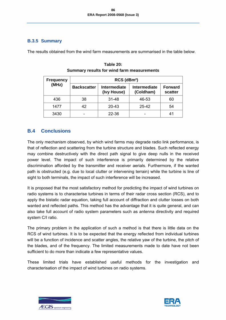
ERA Report 2008-0568 (Issue 3)
86
B.3.5 Summary
The results obtained from the wind farm measurements are summarised in the table below.
Table 20: Summary results for wind farm measurements
RCS (dBm²) Frequency (MHz) Backscatter Intermediate
(Ivy House) Intermediate (Coldham)
Forward scatter
436 38 31-48 46-53 60
1477 42 20-43 25-42 54
3430 - 22-36 - 41
B.4 Conclusions
The only mechanism observed, by which wind farms may degrade radio link performance, is that of reflection and scattering from the turbine structure and blades. Such reflected energy may combine destructively with the direct path signal to give deep nulls in the received power level. The impact of such interference is primarily determined by the relative discrimination afforded by the transmitter and receiver aerials. Furthermore, if the wanted path is obstructed (e.g. due to local clutter or intervening terrain) while the turbine is line of sight to both terminals, the impact of such interference will be increased.
It is proposed that the most satisfactory method for predicting the impact of wind turbines on radio systems is to characterise turbines in terms of their radar cross section (RCS), and to apply the bistatic radar equation, taking full account of diffraction and clutter losses on both wanted and reflected paths. This method has the advantage that it is quite general, and can also take full account of radio system parameters such as antenna directivity and required system C/I ratio.
The primary problem in the application of such a method is that there is little data on the RCS of wind turbines. It is to be expected that the energy reflected from individual turbines will be a function of incidence and scatter angles, the relative yaw of the turbine, the pitch of the blades, and of the frequency. The limited measurements made to date have not been sufficient to do more than indicate a few representative values.
These limited trials have established useful methods for the investigation and characterisation of the impact of wind turbines on radio systems.
ERA Report 2008-0568 (Issue 3)
87
B.4.1 Limitations and further work
The work described suffered from a number of limitations. Perhaps the greatest problem was due to the combination of the low aerial height used (10m above ground) and the flat terrain in the area being measured. Taken together, these ensured that the direct path between transmitter and receiver generally included losses in excess of free space, due to diffraction by foliage, and lack of first Fresnel zone clearance. As any loss on the direct path will tend to exaggerate the relative amplitude of any scattering, the accurate estimation of these losses is crucial to the accuracy of the measurements. In any future work, it would be worthwhile seeking hilltop locations for the terminals to avoid this problem.
The measurements described in this annex were carried out in under four days, and much of this time was spent establishing techniques. Consequently the number of geometries and combinations of turbine yaw and pitch that could be examined were very limited. It might be worth investigating the feasibility of co-operative trials with a turbine operator in which some control might be exercised over the turbine, or, as a minimum, the azimuth, speed and pitch might be logged.