rfq beam cooler injection simulation - mcgill …moore/notes/rfq_injection.pdf · rfq beam cooler...

RFQ BEAM COOLER INJECTION SIMULATION

R.B. MooreJune 16 , 2003

Introduction

Simulating the behaviour of a beam of particles entering a Radiofrequency Quadrupole(RFQ) beam cooler can be a frustrating experience. This is not only because of the large numberof parameters involved in the system design but also because of the large sample of particlesrequired to cover the range of behaviour that they will experience. As in any beam system, thereshould be enough particles to represent the action diagram in one transverse displacement-momentum plane, for at least the initial trial designs. More detailed investigation of a trial designmight even require an investigation of the particle behaviour in the other two displacement-momentum planes. In the case of beam injection into an RFQ system this complexity iscompounded by the fact that particles entering the geometry at different RF phases will experiencevery different fields.

The approach taken here, an approach that is commonly taken in high energy particletransport design, is to start with a linear approximation to the particle dynamics. This allows thesimulation of particle dynamics to be carried out by simple two-dimensional matrix manipulationof not only the action points of individual particles but also of elliptical action diagramsrepresenting whole collections of particles. With modern computers this procedure can lead tosystem evaluation in seconds compared to hours for a higher order calculation.

When in a contemplative mood I think of this approach as following Occam’s razor; “Oneshould not increase, beyond what is necessary, the number of entities required to explainanything”. When contemplating something as prosaic as an RFQ beam cooler I think of it as “Ifit doesn’t work in first order it ain’t going to work in higher order.” (It is only when actuallytesting the system with higher order calculations that one typically encounters the relevantcorollary of Murphy’s Law; “The fact that it works in first order doesn’t mean that it will work inhigher order.)

This description of a linear approach to RFQ beam cooler design centers on a spreadsheetcalculation, written for Excel. The procedure for using this spreadsheet is outlined below, with thetheory behind its creation being reserved for those who actually want to understand it or, morelikely, those who want to do the writer the service of picking holes in it.

The Procedure

Importing Field Maps

The first requirement of the user is to import electric field maps of the components of thecooler system. These field maps have to be created in a separate application. All that is requiredfor the linear approach to charged particle dynamics are the axial field, and the gradient of thetransverse field on the system axis. For the present spread-sheet the maps were created in Simion,which can export the electric field of an electrode configuration at rectangular grid points. Thesewere then imported as columns of electric field and electric field gradients along the axis forcolumnar values of axial grid step.

The present spread sheet is set up to accommodate 10 sets of field maps, each setcomprising a column of DC fields and a column of transverse field gradients. In setting up thesefiled maps for calculations these column must be filled, most conveniently by pasting from anotherspreadsheet or application.

Beam Cooler Injection Simulations 2

As an example, the present spread-sheet is for an electrode system shown schematically infig. 1. In this system there is one field map for the decelerator, which consists of hyperboloidalelectrodes that produce an approximately uniform gradient in the decelerating electric field. Thereare then three maps for three segments of the RFQ confinement system, each segment having thesame RFQ field but with independently adjustable DC potentials.

Fig. 1 The electrodes of a system for decelerating and injecting a high voltage DCbeam into an RFQ confinement region. The particles enter the decelerator through ahole in the ground electrode, this electrode being a hyperboloid of revolution. Themain decelerating electrode is a ring, shown to be at 63750 V in the figure, that isalso a hyperboloid of revolution. This ring is configured so as to produce aequipotential cone at 60000 V, with its apex at zO from the center of the groundelectrode and consequently a purely quadrupole field in the deceleration region. Thethird deceleration electrode is a cone that follows this equipotential surface, but witha hole to allow the particles to enter the RFQ confinement region, which is insidethe cone. In the configuration shown in the figure the RFQ confinement region hasthree segments set at different DC ptotentials, thereby allowing the axial energy ofthe particles to be modified after their entry into the system.

For this example spreadsheet the 3 separate sequential sets of quadrupole electrodes, shownin fig. 1 and in more detail in fig. 2, are all calculated with the same grid spacing andsuperimposed on one grid axis extending over 163 points, counting zero. Here the imported


fields are the axial electric fields (in Volts per step) and the transverse field gradients (in Volts perstep2).

Fig. 2 The configuration of the RFQ electrodes

Not all the field maps need be filled so the spreadsheet requires that the number that areactually used be entered in the cell “Number of maps”. Then for each map that is entered thefollowing information must be entered in the appropriate cells:

A. The number of rows in the map.

B. The number of steps in a key dimension of the map (“Key Dim. – steps”) This couldbe simply the number of steps in the field map, i.e. the number of rows as above, but itcould also be an easily recognized feature of the electrode configuration such as thedistance of a set of quadrupole elements from the axis (i.e. “ro”).

C. The potential on a key electrode for which the axial DC field map was calculated (“Calc.DC Pot”). If there is only one activated electrode then the potential is, of course, thepotential of that electrode. However, if there is more than one electrode for thecalculation, and which will therefore always have the same potential ratios, then the mosteasily recognized electrode could be selected.

D. The potential on a key electrode for which the transverse field gradient map wascalculated (“Calc. RF Pot”). Here there will always be more that one electrode and sothe most easily recognized electrode should be selected.

E. A flag to indicate that there is a transverse field gradient map (“Quad. Field?”). If thiscell contains zero there is none.

In addition the user must provide the information required to set the geometrical andelectrical scales of the maps. These are most conveniently entered in the appropriate cells asformulae referring to more easily visualized parameters in the main header of the spreadsheet. The required entries are:


F. “Key Dim. – mm” - The length in mm of the key dimension entered as steps in B. Inthe present spread sheet the entry for field maps 2, 3 and 4 are the ro (in mm) of theelectrode configurations. This is set by the user in cell “ro (mm)” as part of any trialcalculation. This entry is given the variable name “ro” which has been entered in theformulae for “Key Dim. – mm” of each of the maps. The spreadsheet then calculatesthe scale factor by dividing this “Key Dim. – mm” by “Key Dim. – steps”.

G. “ zstart” – The z coordinate at which the field map starts. This can be set in theappropriate cell above the field map but is often most conveniently set from informationentered in cells in the main header of the spreadsheet. In the present spreadsheet it is setto zero for the first field map (the decelerator) and for the 2nd , 3rd and 4th as a formularelating it to the entry into the cell “Quad map start” in the main header. Thespreadsheet then calculates “zend” using the number of steps in the field map and thescale factor.

H. “Set DC Pot.” The potential on the key electrode for which the axial DC field map wascalculated. As an example, in the present spreadsheet for map 1 this potential is enteredas being equal to the entry in the cell “Decel. Pot” in the main header.

I. “Set RF Pot.” The potential on the key electrode for which the transverse field gradientmap was calculated. As an example, in the present spreadsheet for map 2 this potentialis entered as a formula linking it to the entry in the cell “RF ampl” in the main header.

Note that the units used in the spread-sheet are millimeters, Volts and microsconds. For ashort guide to these units, and a sermon about their overwhelming usefulness, see the Appendix.

Also note that for the example spreadsheet the same quadrupole field is applied to eachelectrode set, so these have already been compiled and entered in the 2nd transverse field map. Theother 2 quadrupole electrode sets are then set to have no have transverse field.

The calculation of the electric field maps and their insertion into the spread-sheet are by farthe most laborious part of using the spread-sheet. This is particularly true if one has to introducenew electrodes. This is a usual feature of particle manipulation design schemes, where a change inthe geometry of a system is the highest iteration to be performed. One therefore tries to do asmuch as possible with a particular geometry before altering it. The purpose of this spread-sheetbased on first-order beam optics is to bring into balance the time required to exhaust thepossibilities of a particular design through lower level iterations with the time required to introducea new iteration requiring a shape change of the system.

Compiling the Field Maps

Once the field maps and their associated parameters are entered in the spreadsheet macrosmust be activated to calculate the spline coefficients needed for the interpolations required forassembling the fields into one overall field map. The first of these is the macro“FillFieldsArray”, which enters the spline coefficients in the field map arrays. This is activatedby pressing Cntl-f (or Option+Command+f on a Macintosh) and must be run following anychange in a field map and any change in the geometric scale and/or the relative placement of thefiled maps. This operation should take less than a second on a modern personal computer.

The second macro needed for the field compilation is “FillCombFieldArray”, activated bypressing Cntl-c (or Option+Command+c on a Macintosh). This takes the field map data, togetherwith the set potentials, and uses spline interpolations to calculate the combined field. It enters


these field values, together with the spline coefficients required for their interpolation, in the array“CombFieldArray”. This field map is in 500 uniform axial steps over its entire extent. Thismacro must be run whenever a set potential is changed, or whenever macro “f” is run.

The Runge-Kutta Integration

The use of matrix algebra for the linear approximation of beam dynamics requires accurateknowledge of the axial coordinate of the particle collection at particular times. For the large rangeof energies involved in decelerating a particle beam from typically 60 keV to entry into RFQconfinement at the order of 10 eV, the required accuracy can only be obtained from higher ordercalculations. In the present spreadsheet the necessary accuracy is acquired through a 5th orderRunge-Kuttas integration of the equations of motion of a particle traveling along the z axis of thesystem, with spline interpolation of the axial electric fields that govern this motion. However,because of the errors that accumulate in the potentials at grid points in any field calculationprocedure (in the words of “Numerical Recipes”, resulting in a “rocky terrain”), even with thesemeasures errors of the order of 10 eV compared to conservation of energy have been observedwhen the particle energy has been reduced from 60 keV to this range. For this reason the Runge-Kutta integration as applied here overwrites the value of the particle velocity calculated at the endof each step of the integration with the value calculated from conservation of energy and theelectric potential of the position at the end of that step.

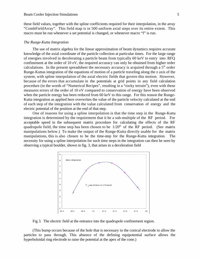
One of reasons for using a spline interpolation is that the time step in the Runge-Kuttaintegration is determined by the requirement that it be a sub-multiple of the RF period. Foracceptable speed in the subsequent matrix procedure for calculating the effects of the RFquadrupole field, the time step has been chosen to be 1/20th of the RF period. (See matrixmanipulations below.) To make the output of the Runge-Kutta directly usable for the matrixmanipulations, this is also chosen to be the time-step for the Runge-Kutta integration. Thenecessity for using a spline interpolation for such time steps in the integration can then be seen byobserving a typical boulder, shown in fig. 3, that arises in a deceleration field

Fig 3. The electric field at the entrance into the quadrupole confinement region.

(This bump occurs because of the hole that is necessary in the conical electrode to allow theparticles to pass through. This absence of the defining equipotential surface allows thehyperboloidal ring electrode to raise the potential at the apex of the cone.)


In this figure the squares represent the values of the axial field at the axial points representedin the z column of the combined field data that is used in the integration. The curve drawn throughthem is the spline interpolation as used in the Runge-Kutta integration. It is seen that a linearinterpolation from point to point would cause noticeable error in the value of the electric field thatthe Runge-Kutta would be using., and this would be at a very critical point in the manipulation ofthe particle beam through the hole.

In principle, the necessity of a spline interpolation could be eliminated by using a muchshorter time interval for the Runge-Kutta than that used for the matrix manipulations. The resultscould then be made directly usable for the matrix manipulations by having the time-interval of theRunge-Kutta a sub-multiple of that used for the matrix manipulations and only outputting to theRK array data at the matrix intervals. However, this would involve considerably moreprogramming of the Runge-Kuttta algorithm and/or would considerably slow the Runge-Kuttaprocess itself, with no appreciable gain in accuracy over using the spline interpolation.

The particle parameters required for the Runge-Kutta integration are entered in the cellsunder “Incoming Beam”. Specifically, these are the ion mass in atomic mass units (“Ion mass(amu)” and the beam energy in electron volts (“Energy (eV)”). The Runge-Kuttta integration isthen done by the macro “FillRKArray”, activated by pressing Cntl–k (or Option+Command+kon a Macintosh). This subroutine fills RK_Array with the values of time (“t”), z, (“z”), z-velocity, (“zdot”), particle axial energy (“KE”) and the axial electric field (“Ez”) at these zvalues. For reference it also fills in the estimates of the errors in z and ˙ z associated with each stepthat are a by-product of the 5th order Runge-Kutta algorithm. (See “Numerical Recipes”.)

The FillRKArray macro also calculates the values needed for the matrix manipulations,specifically the axial derivative of the axial field (column “dEz/dz”), the transverse field gradienton the axis (column “dRr/dr”) and the axial gradient of this transverse field gradient (column“d2Rr/drdz”).

The beam parameters needed for the first-order matrix calculations of the beam envelope areits emittance (cell “ξ−(π–mm-mrad)” ), diameter (cell “Diameter (mm)”) and angular spread(cell “Angular spread (mrad)”). (A negative angular spread indicates a beam converging onto theentrance of the field map).

The spread-sheet is now ready for the first-order calculation of the beam profile through thesystem and an estimate of axial energy effects.

The Matrix First-order Calculation

The first-order matrix calculation of the beam profile is carried out by the macro subroutine“FillResultArray”. This can be activated by pressing Cntl-b (or Option+Command+b on aMacintosh). It uses 2-dimensional matrices to calculate the transformation of this ellipseparameters at each time step of the Runge-Kutta output. The ellipse parameters that are actuallytransformed are the so-called “Twiss Parameters” – see “Theory” section below.

An estimate of the effects on the axial energy of the axial gradient of the transverse fieldgradient is obtained by running the macro “FilldEArray” also see “Theory” section. This canbe activated by pressing Cntl-e (or Option+Command+e on a Macintosh). A spectrum of thisestimated energy deviation is obtained from the macro “filldNdEArray” that can be run bypressing Cntl-n (or Option+Command+n on a Macintosh). (This macro is run automatically as asub macro in “e” but the option of running it separately on previously compiled data from “e”allows different scales of the spectrum to be obtained by minor modifications of the code of “n”.)

The percentage of the beam estimated to be in the displayed spectrum is shown in the cell“% of beam”


Theory

Action Diagrams

The power of action diagrams in analyzing the motions of a particle collection seems to havebeen first realized by Poincaré at the turn of the 20th century, and such diagrams are sometimesreferred to as “Poincaré sections”. Their power derives from the fact that they are projections ofthe momentum-displacement coordinate pairs for each degree of freedom of the particle motions.Thus to first order, where the motion in each degree of freedom is independent of the motion inthe others, the preservation of the particle density in phase space, and hence the preservation of thephase space volume of a collection (Liouville’s Theorem), leads to preservation of the density andthe area of the action diagrams. (This property of particle collections in conservative systems issometimes expressed as “the incompressibility of particle collections in phase space”.)

Since the electric field of a quadrupole is linearly related to particle displacement in that field,the forces have always first-order dependence on displacement and so the action diagrams of aparticle collection retain their local density and overall area.

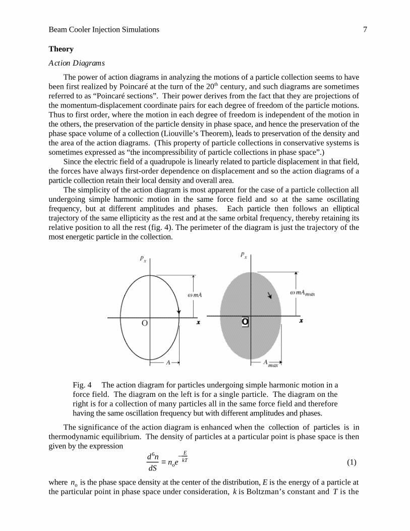
The simplicity of the action diagram is most apparent for the case of a particle collection allundergoing simple harmonic motion in the same force field and so at the same oscillatingfrequency, but at different amplitudes and phases. Each particle then follows an ellipticaltrajectory of the same ellipticity as the rest and at the same orbital frequency, thereby retaining itsrelative position to all the rest (fig. 4). The perimeter of the diagram is just the trajectory of themost energetic particle in the collection.

Fig. 4 The action diagram for particles undergoing simple harmonic motion in aforce field. The diagram on the left is for a single particle. The diagram on theright is for a collection of many particles all in the same force field and thereforehaving the same oscillation frequency but with different amplitudes and phases.

The significance of the action diagram is enhanced when the collection of particles is inthermodynamic equilibrium. The density of particles at a particular point is phase space is thengiven by the expression

d6n

dS= noe

− EkT (1)

where no is the phase space density at the center of the distribution, E is the energy of a particle atthe particular point in phase space under consideration, k is Boltzman’s constant and T is the


temperature of the collection. For simple harmonic motion, where the energy is divided betweenthe potential energy of displacement and the kinetic energy of the momentum, the projection ofthis density distribution into an action diagram results in a gaussian density distribution within thatdiagram given by

d2n

dxdpx

= nA oe

− x2

2σ x2

+ px2

2σ px2

(2)

where nA o is the density distribution at the center of the action diagram and the standarddeviations of the distribution are

σx =1

ωkT

m , σpx

= mkT . (3)

The action diagram for the distribution will then be elliptically symmetrical in that points anywhereon the ellipse representing a particular amplitude of oscillation will have a uniform density.

Matrix Algebra of Action Diagrams

The transformation of a point in an action diagram as the diagram evolves under lineartransformations is described by the 2-dimensional matrix M

x

px

′= M

x

px

, M =

m11 m12

m21 m22

. (4)

A consequence of the linearity of the transformation is that the determinant of this matrix is unity.Also, the elements of the inverse transfer matrix

x

px

= M−1 x

px

′ (5)

can be easily determined from the simple requirement

M−1M =1 0

0 1

to be M−1 =

m22 −m12

−m21 m11

(6)

where the elements m11, m12 , m21 and m22 are those of the forward transform.In the case of an ion in an axisymmetric quadrupole field with axis of symmetry along the z

axis the electric potential has the form

φ =a

2z2 −

1

2r2

. (7)

This potential has a radial electric field

Er =−a

2r . (8)

which results, of course, in a radial oscillation of frequency

ω =ea

2m (9)


where e is the charge and m is the mass of the ion. The radial displacement and radial momentumare then

r = A sin(ωt + φ) , pr = mωAcos(ωt + φ) . (10)

In the case of the quadrupole being negative, resulting in a radial field that is away from the zaxis, the motion becomes

r = A sinh(ωt + φ) , pr = mωAcosh(ωt + φ) (11)

where now the magnitude of the quadrupole field is used in evaluating ω.These solutions result in the transformation of the displacement-momentum coordinates

during an interval t being expressed by the matrices

M+ = cos(ωt)1

mωsin(ωt)

−mω sin(ωt) cos(ωt)

, M− = cosh(ωt)

1mω

sinh(ωt)

mω sinh(ωt) cosh(ωt)

(12)

For these matrices the determinants are easily seen to be unity and the inverse matrices,describing a transformation in negative t, are easily seen to follow eqn. (6).

For a field that is not purely quadrupolar the linear approach can be used by taking smallsteps through the system. In the linear approach the field over a small step can be taken asquadrupolar. This means that if there is an axial field gradient in this step then there is also atransverse field gradient

∂E r

∂r=−

1

2

∂Ez

∂z . (13)

The elemental transformation matrice for a step that takes time dt is then

dM+ = cos(ωdt)1

mωsin(ωdt)

−mω sin(ωdt) cos(ωdt)

(14)

when the axial field gradient is positive and

dM− = cosh(ωdt)1

mωsinh(ωdt)

mω sinh(ωdt) cosh(ωdt)

(15)

when the axial field gradient is positive, and where

ω =e

2m

∂Ez

∂z . (16)

Elliptical action diagrams are of particular significance in linear transformations since theyremain ellipses of the same area. Linear transformations of ellipses are most convenientlyexpressed in terms of the Twiss parameters A, B, C and ε , by which the equation for an ellipse,in terms of the coordinates of its points relative to its center, has the general form

Cx 2 + 2Axy + By2 =ε . (17)

For an action diagram it has the specific form

Cx 2 + 2Axpx + Bpx2 =ε . (18)


The parameter ε determines the overall size of the ellipse. Specifically, it is the product of thesemi-axes, or Area of ellipse /π Thus, defining the action as the area of the action ellipse, it isAction /π The parameters B and C express the ellipticity of the ellipse. The parameter Aexpresses the inclination of the ellipse axis with the axis of the coordinate system and is zero whenthe ellipse is a right ellipse. Because it takes only 3 parameters to specify any ellipse there is anecessary relationship between the Twiss parameters. It is

BC − A2 =1 (19)

The relationship of the Twiss parameters to the cardinal points of an ellipse is shown infig. 5.

Fig. 5 The relationship of the Twiss parameters of an ellipse to the variouscardinal points of the ellipse and its orientation with the coordinate axes.

As an example, the Twiss parameters for the action ellipse of simple harmonic motion are

A = 0, B =1

mω, C = mω, ε = mωxmax

2 . (17)

Because a linear transformation preserves the area of an ellipse, only the parametersA, B and C are transformed. The 3 × 3 matrix that describes this transformation, and its inverse,for an action point transformation described by the 2 × 2 matrix of (4) are


B

A

C

′

=m11

2 −2m11m12 m122

−m11m21 m11m22 + m12m21 −m12m22

m212 −2m21m22 m22

2

B

A

C

(18)

B

A

C

=

m222 2m12m22 m12

2

m21m22 m11m22 + m12m21 m11m12

m212 2m11m21 m11

2

B

A

C

′

. (19)

If the electric field is static then the envelope of a beam traveling along the axis of the systemcan be obtained by determining the step by step transformation of the B action parameter andusing the relationship shown in fig. 5:

rmax = εB . (20)

Action Diagrams of RFQ Confinement

The case of the oscillating quadrupole field that provided radial confinement is morecomplicated. Here the frequency ω is itself varying and so, strictly speaking, the transformationmatrices (14,15) are only valid for infinitesimal time intervals. The transfer matrix for a finite timet is then the product sum

M =Π tdM, (21)

In principle this product sum should be evaluated over infinitesimal time steps, or an infiniteset of dM. In practice, for quadrupole field strengths that are oscillating sinusoidally, time steps of1 degree of oscillation will give accuracies of several parts in 105 and steps of 5 degrees will giveaccuracies of about 1 part in 103.

Thus, even in the linear approach sufficient accuracy is achieved only with many steps perfield oscillation. To circumvent this problem the combination of many small steps into largersteps can be carried out beforehand and the results compiled for interpolation during the actualbeam profile calculations. This is facilitated by describing the sinusoidal variation of the field interms of the angle of the variation rather than the time;

dEr

dr=

dEr

dr

max

sin θRF( ) . (22)

whereupon the equation of motion becomes

d2r

dθRF2 =

e

mωRF2

dEr

dr

max

sin θRF( )

r . (23)

Using the dimensionless Mathieu parameter

q = 2e

mωRF2

dEr

dr

max

. (24)

(23) takes the simple form

d2r

dθRF =

q

2sin θRF( )

r . (25)


The elemental transfer matrix for a small step in θRF is then

dM+ =

cosh(q

2sin(θRF )

1

2dθRF)

1

q

2sin(θRF )

12

sinh(q

2sin(θRF )

1

2dθRF)

q2

sin(θRF)

12

sinh(q2

sin(θRF)

12

dθRF ) cosh(q2

sin(θRF)

12dθRF )

(26)

for 0 ≤θRF ≤ π , and

dM− =

cos( −q

2sin(θRF )

12

dθRF)1

q2

sin(θRF )

12

sin( −q

2sin(θRF)

12

dθRF)

− −q2

sin(θRF )

12 sin( − q

2sin(θRF)

12 dθRF ) cos( − q

2sin(θRF)

12 dθRF)

(27

for π ≤θRF ≤ 2π

These elemental transfer matrices can then be combined to yield the transfer matrices forlarger steps. For the beam envelope calculations this has been done in a separate spread-sheet(“RF_Matr_fract_cycle.xls”) for values of q in steps of 0.1 from 0 to 3.0 and for steps in θRF of18o starting at 0 and ending at 360o. These results were pasted into the beam envelope spreadsheetas arrays “M11ARRAY”, “M12ARRAY”, “M21ARRAY” and “M22ARRAY”.

This allows an evaluation of the matrix elements for an 18o step through the RFQconfinement regions by determining the average q during that step and using interpolation to findthe θRF matrix elements for that step. The matrix elements for the transformation according to theequation of motion in time can then be obtained from

m11 = m11θ ; m22 = m22θ

m12 =m12θ

mωRF ; m21 = mωRF( )m21θ

. (28)

Combining the Axial Gradient and the RFQ Transformations

The axial field transformation (14,15) and the transverse field transformation derived from(26,27) both include the effect of the axial drift during a step. In combining these transformationsone then has to unwind the effect of one of these drifts. For example, if the axial fieldtransformation is taken to be the first then the simple drift part of its transformation must beundone before the transverse matrix is applied, as in (29).

∆MStep =m11trans

m12 trans

m21transm22trans

×1 −∆t

m0 1

×

m11axialm12axial

m21axialm22axial

(29)


Axial Energy Effects of the RFQ Fringe Field Region

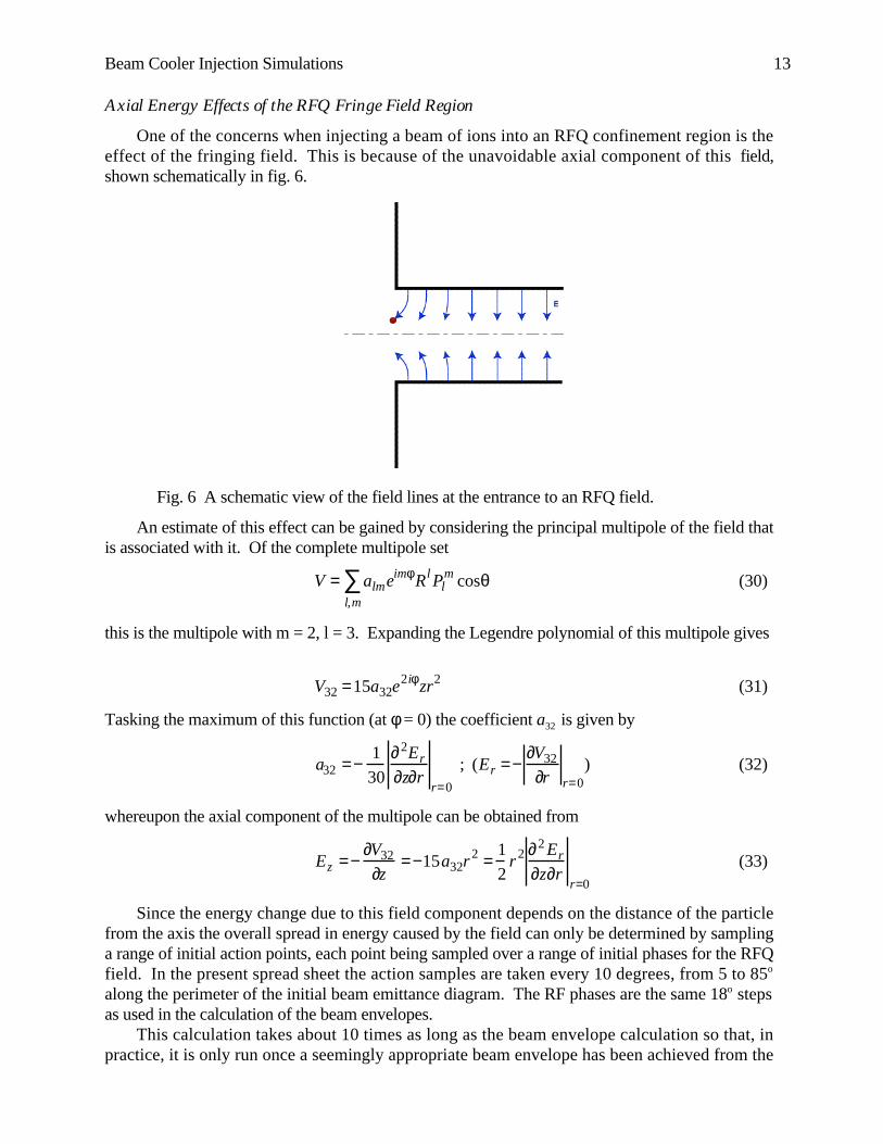
One of the concerns when injecting a beam of ions into an RFQ confinement region is theeffect of the fringing field. This is because of the unavoidable axial component of this field,shown schematically in fig. 6.

Fig. 6 A schematic view of the field lines at the entrance to an RFQ field.

An estimate of this effect can be gained by considering the principal multipole of the field thatis associated with it. Of the complete multipole set

V = almeimφ

l,m

∑ Rl Plm cosθ (30)

this is the multipole with m = 2, l = 3. Expanding the Legendre polynomial of this multipole gives

V32 =15a32e2iφzr2 (31)

Tasking the maximum of this function (at φ = 0) the coefficient a32 is given by

a32 =−1

30

∂2Er

∂z∂rr=0

; (Er =−∂V32

∂r r=0) (32)

whereupon the axial component of the multipole can be obtained from

Ez =−∂V32

∂z=−15a32r 2 =

1

2r 2 ∂2 Er

∂z∂rr=0

(33)

Since the energy change due to this field component depends on the distance of the particlefrom the axis the overall spread in energy caused by the field can only be determined by samplinga range of initial action points, each point being sampled over a range of initial phases for the RFQfield. In the present spread sheet the action samples are taken every 10 degrees, from 5 to 85o

along the perimeter of the initial beam emittance diagram. The RF phases are the same 18o stepsas used in the calculation of the beam envelopes.

This calculation takes about 10 times as long as the beam envelope calculation so that, inpractice, it is only run once a seemingly appropriate beam envelope has been achieved from the


beam envelope calculation. Since the effect on the energy is proportional to the square of thedistance of the particle from the axis it is important to get as small a beam diameter as possible inthe RFQ entrance region.

This effect on the axial energy will, of course, render the RK integration based on the axialvalues of the field inaccurate. Therefore. if the energy calculations indicate an unacceptable effectthe RK calculations on which they were based cannot be trusted and so the iterations must berepeated until the energy spread is indeed acceptable.

An estimate of the spectrum of the energy spread due to the axial gradient of the transversefield gradient can be obtained by assuming that the density of the initial action diagrams of theincoming beam corresponds to thermal equilibrium. If the emmittance used in the calculationencompasses 90% of the total thermally equilibriated beam (a common practice in beam optics )then the action density will be

dN

dA=

dN

dA

o

e−2.3

r 2

ro2

(34)

where the “radius” parameter r is the distance of the action point from the action diagram centerwhen the momentum coordinate is given the same dimensions as the displacement coordinate (i.e.the ellipse has been scaled into a circle) and rois the radius of the “emittance” ellipse.

For a pie shaped slice of angle ∆θ of this emittance diagram the density of particles as afunction of radius will be

dN

dr=

dN

dA

o

r∆θ e−2.3

r2

ro2

. (35)

For any given initial action point, the energy deviation caused by the fringe field of thequadrupole will be proportional to the square of the initial r parameter of the action. For theparameter value ro let the energy deviation be designated Eo. The spectrum of the energy deviationfor the particles contained within the slice then becomes

dN

dE=

N

Eo

e−2.3

E

Eo (36)

where N is the number of particles in the slice represented by the segment at the perimeter of theemittance ellipse. For thermal equilibrium and uniform slice angles this number is the same for allsegments around the perimeter. Also, the density of the initial action diagram will not depend onthe phase of the RF at which it enters the system. The total spectrum of all the incoming particlescan then be obtained by summing

dN

dE

Total

= nN

Eo

e−2.3

E

Eo∑ (37)

where the sum is taken over all the initial action points and all the RF phase for each action point.Hence n is the product of the number of action points and the number of phase samples.

However, this method of sampling the initial action points assumes that the initial actionellipse is a right ellipse that can be rendered into a circle by a simple scale change of itsdisplacement and momentum coordinates. The actual incoming beam will in general have anellipse that is inclined to the displacement-momentum axis. The application of this method of


sampling action points therefore requires that the right ellipse from which they are sampled betransformed into the actual emittance ellipse of the incoming beam.

The right ellipse that is taken for the initial azimuthally uniform sampling can be taken to bethe actual beam emittance ellipse simply rotated to be a right ellipse. Taking the Twiss parametersof this right ellipse to be B’ and C’ (A’ = 0) then the transformation of that right ellipse to theactual entrance ellipse specified by Ao, Bo and Co becomes

Bo

Ao

Co

=m11

2 −2m11m12 m122

−m11m21 m11m22 + m12m21 −m12m22

m212 −2m21m22 m22

2

′ B

0

′ C

. (38)

resulting in

Bo = m112 ′ B + m12

2 ′ C . (39)

Given that the elements of the transfer matrix that results in a simple rotation are simply

m11 = m22 = cosθm12 =−m21 = sinθ

(40)

where θ is the angle of rotation. This results in

m11 = m22 = Bo − ′ C

′ B − ′ C

1

2

m21 =−m12 = 1− m112

(41)

The Twiss parameter B’ and C’ can be obtained from the semiaxis of the actual emittanceellipse (see fig. 5) that will become the semi-axis of the right ellipse (as pxmax). The result is

′ C = 1

2Bo + Co + (Bo + Co)

2 − 4( )′ B = 1

′ C

(42)

The semiaxis of the right emiitance ellipse from which the action samples are to be taken arethen

px max= ε ′ C ; xmax = ε ′ B (43)

and the coordinates of the action sample points become

px i= pxmax

sinθ i ; xi = xmax cosθi (44)

These sample points are then transformed to the action at beam entrance according to

px

x

Entrance

=m11 m12

m21 m22

px

x

Sample

(45)


Tests

The accuracy of the present spread-sheet calculations can only be adequately tested bycomparing its results with those of an accurate ray-tracing program for particles traversing thesame fields. However, tests of the matrix components in tables M11ARRAY etc. indicate anaccuracy of about 1 ppm, with the accuracy of values interpolated from these tables estimated to benever worse than 10 ppm. When applied in the sequence of steps required for the beam envelopecalculation it is expected that the final beam envelope should be accurate to of the order of 1%.

Gross errors have been checked by following the trace of a single particle and comparing itwith what would be expected from general considerations. The axial transformation part of thecalculation was checked by the behaviour of a particle starting at maximum displacement and nodivergence upon entrance to the decelerator. In the predominately quadrupole field of thedecelerator the action point of this particle should trace out a right ellipse, the semiaxes being

xmax = xinitial

pxmax = mωxmax =em

2

dEz

dz

. (46)

For a particle of 100 amu entering parallel to the z axis and 3.5 mm from it, a purequadrupole field that is 60000V at a distance z = 50 mm from its center of zero potential at z = 0,results in

xmax = 3.5 mm

pxmax =17.5 ev -µs/mm . (47)

The action trace produced by the spread-sheet is shown in fig. 7

Fig. 7 The action trace of an ion of mass 100 amu entering the almost purequadrupole field of the decelerator modeled in the spread sheet calculations. Thetrace is seen to be a right ellipse with the expected semiaxes. The slight flattening atthe bottom and the subsequent turn-up near the end of the trajectory is due to theparticle approaching the entrance hole of the RFQ section and then entering thefield-free region inside. (The RFQ field was set to zero for this calculation.)


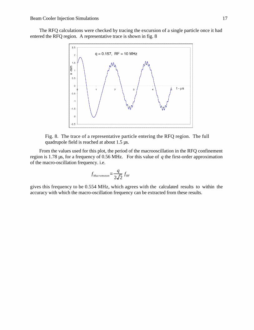
The RFQ calculations were checked by tracing the excursion of a single particle once it hadentered the RFQ region. A representative trace is shown in fig. 8

Fig. 8. The trace of a representative particle entering the RFQ region. The fullquadrupole field is reached at about 1.5 µs.

From the values used for this plot, the period of the macrooscillation in the RFQ confinementregion is 1.78 µs, for a frequency of 0.56 MHz. For this value of q the first-order approximationof the macro-oscillation frequency. i.e.

fMacromoton =q

2 2fRF

gives this frequency to be 0.554 MHz, which agrees with the calculated results to within theaccuracy with which the macro-oscillation frequency can be extracted from these results.


APPENDIX A - SPREAD SHEET GLOSSARY

Names used in the spread sheet

Name Spread-sheet

label

Description User modified

or internal calc.

Ao Ao Emittance Twiss parameter A at startInternal

Bo Bo Emittance Twiss parameter B at startInternal

Centerz Centerz The z coordinate of the dec quad centerInternal

Co Co Emittance Twiss parameter C at startInternal

CombFieldArray Interpolated- 6 column array of fields used in calc.Array

DCpot1-10 Calc. DC Pot. Potentials used in calculating fieldsUser

dEArray Energy dev- 20 column array of energy deviationsArray

DecelPot Decel-- Set potential of decelerator User

dEdNArray Energy Spec- 2 column array of energy spectrumArray

deltaEpercent % of beam - % of beam in displayed E spect. Internal

deltat ∆t – (µs) Time interval used in RK calculationsInternal

deltaTheta Angular spread Beam divergence at start (mrad) User

Diameter Diameter (mm) Beam diameter at start User

El1_DC Electrode 1-DC Set DC on first quad User

El2_DC Electrode 2-DC Set DC on 2nd quad User

El3_DC Electrode 3-DC Set DC on 3rd quad User

Emittance ξ (π-mm-mrad) Beam emittance User

Energy Energy (eV) Particle kinetic energy at start User

Entrancez Entrancez Z coordinate at entrance to decel. region Internal

epsilon epsilon Emittance Twiss parameter ε at start Internal

FieldMapArray ELECTRODE - 50 column field map array (5 per map)Array

freq MHz Frequency of RF User

Ion_mass_amu Ion mass (amu) Particle mass in amu User

Ion_mass_imu Ion mass (imu) Particle mass in “ion mass units” Internal

keydim1-10 Key Dim. -StepsKey dimension for scale of maps User

keydim1-10_mm Key Dim. mm Set key dimension for scale User

M11ARRAY M11ARRAY Tabulated m11 RFQ matrix elementsArray




MapDataArray Map Data Ar- Collected array of field map param.Array

momega momega Product of mass and RF radian freqInternal

momegasqr momegasqr Product of mass and RF rad. freq. sqr.Internal

Nelectrodes Number of mapsNumber of field maps Entered with map

nrows1-10 No of rows Number of rows in field maps Entered with map

Nsteps No of Plot stepsNumber of steps in the RK calculationUser

omega omega Angular frequency of the RF Internal

q q Mathieu parameter for the RFQ fieldInternal

Quad._Field1-10?Quad. Field? If there is a quad field, 1 else 0 User

ResultArray r boundary - 41 column array of beam envelopesArray

RF_ampl RF ampl Amplitude of RF across adjacent elect.User


RFpot1-10 Calc. RF Pot. RF potential for calculating maps Entered with map

RK_Array RK_Array 10 column array of Runge-Kutta calc.Array

ro ro (mm) The distance of the RF electr. from axisUser

scale1-10 mm/step) The scales of the field maps Internal

SetDCPot1-10 Set DC Pot. DC potentials used in beam calculationsUser

SetRFpot1-10 Set RF Pot. RF potentials used in beam calculationsUser

zconfstart Quad map start z coor. at start of the quad field mapUser

zend1-10 zend z coordinates at end of field maps Internal

zo Decel. zo Actual zo parameter used in calculationUser

zstart1-10 zstart z coordinates at start of field mapsUser

User defined functions in the spread sheet

Interpolate(xlow, xhigh, ylow, yhigh, x)A linear interpolation routine used to calculate the electric potentials required for thevelocity determinations in the subroutine FillRKArray

Spline(xlow, xhigh, ylow, yhigh, y2low, y2high, x)A spline interpolation routine used to calculate electric fields.

Macros used in the spread sheet

FillFieldsArray() - Activated by Ctrl-f (Option+Command+f on the MacIntosh)A macro to compute the column of spline derivatives needed to interpolate the electricfield maps for the beam calculations. Need to be activated when importing a new fieldmap or changing the geometrical scales and/or field map starting points.

FillCombFieldArray() - Activated by Ctrl-c (Option+Command+c on the MacIntosh)A macro to compute the combined field of the field maps, taking into account the user setpotentials. Needs to be activated when an electric potential is changed (or “f” is run).

FillRKArray() - Activated by Ctrl-k (Option+Command+k on the MacIntosh)A macro to carry out the Runge-Kutta integrations for the particle position on the axis vstime. It uses time steps set to be 1/20 of an RF cycle. Needs to be activated whenparticle energy or mass is changed, or “c” is run).

FillResultArray() - Activated by Ctrl-b (Option+Command+b on the MacIntosh)A macro to compute the beam envelopes at the RK step points. Needs to be activatedwhen beam emittance, diameter or divergence has been changed (or “k” has been run).

FilldEArray()- Activated by Ctrl-e (Option+Command+e on the MacIntosh)A macro to compute the estimate of the axial energy spread. Needs to be run whenever“b” has been run

FilldNdEArray()- Activated by Ctrl-n (Option+Command+n on the MacIntosh)The macro used within FilldEArray to compute the spectrum of the axial energy spread.Can be run separately if a different energy scale is desired in the spectrum disply.(Would require editing the macro.)


APPENDIX B - RFQ ACTION DIAGRAMS

Introduction

The motion of charged particles under RadioFrequency Quadrupole (RFQ) confinement canseem confusing. This is because of the combination of the driven oscillation of the oscillatingelectric field, which produces an oscillation in which the displacement is in antiphase to the forceoscillation of the quadrupole, and the underlying simple harmonic motion from the averagerestoring force that the oscillating field produces. The result, for a single particle in a typicaloscillating quadrupole field used for confinement is shown in fig. A1.

Fig. A1 A typical motion of an ion in one dimension under RFQ confinement.

Although this motion may appear relatively simple for a single ion in one dimension of itsmotion, the motion in space, even for the 2-dimensional radial confinement of an ion guide, canresult in a tortuous path because of the lack of any coherent phase relationship between the drivenoscillation and the independent simple harmonic motions in the spatial coordinates x and y. Atypical trajectory for a single ion under RFQ radial confinement is shown in fig. A2.

Fig. A2 A typical trajectory of an ion under 2-dimensional RFQ confinement.


If there is more than one ion under confinement than the motions form an even more tangledweb (fig. A3).

Fig. A3 A typical motion of two ions under 2-dimensional RFQ confinement.

All that is easily discerned about the trajectories of a large collection of ions is that they fill asquare of rounded corners, the diagonals of the square being oriented along the directions of themaximum quadrupole electric potentials (i.e. x and y in fig. A3). Yet, this confusing collections ofmotions must be dealt with analytically if RFQ confinement is to be designed for particularapplications, such as the preparation of ion collections for delivery to other apparatus for furtherstudy. An example is the use of RFQ confinement while ion collections are being cooled bybuffer gas collisions for delivery to a high-accuracy mass spectrometer, where the cooling of theions is a necessary prerequisite for the high-accuracy. An appropriate analysis of the ion motionsis obtained by considering the action diagrams, i.e. momentum-displacement, of the motions.

Action Diagrams of RFQ Confinement

Since the driven RF oscillation of particles under RFQ confinement is superimposed on theirsimple harmonic motions the action diagrams of a collection of particles will be that of simpleharmonic motion to which the RF motion is added. However, unlike the simple harmonic motion,the RF motion will not be at arbitrary phase but will always be in antiphase to the electric field.The particles will therefore not fill the ellipse of the most energetic oscillation, as in their simpleharmonic motions, but rather will form a line which rotates within that ellipse, one complete turnfor each RF cycle (fig. A4).


Fig. A4 Action diagrams for a collection of particles undergoing driven oscillationsin an oscillating force field. The diagram on the left is for an RF phase of zero(zero electric field but going positive). The diagram in the middle is for an RFphase of 45 degrees and the diagram to the right is for the force field at maximumvalue.

The effect of the addition of this sort of action to the simple harmonic motion of the RFQconfinement is to distort the ellipse of the simple harmonic motion into ellipses that are specific tothe phase of the RF, as shown in fig. A5.

Fig. A5 Action diagrams for RFQ confinement in which the action of the drivenRF oscillation is combined with the underlying simple harmonic motion.

Because the quadrupole field is a linear (first-order) force field, in which the forcecomponents are proportional to the displacement components, the distortion it applies to thesimple harmonic motion action ellipse keeps it elliptical and of the same area.

Thus the full motion of a collection of particles under RFQ confinement can be described asa rotation within an ellipse that is itself being constantly deformed in the manner shown in fig. A5,with the deformation repeating each RF cycle. Analysis of the motion then involves expressingthis deformation mathematically. Because the transformations of the action diagrams for RFQconfinement are linear this is most easily accomplished using matrices in linear algebra. (For afull description of the use of matrix algebra for the transformation of action diagrams see [1] andreferences contained therein.)


Matrix Algebra of the Action Diagrams of RFQ Confinement

In can be shown that for a linear transformation specified by the elementsm11, m12 , m21 and m22 the eigensolution for the Twiss parameters, i.e. the set of parametersdescribing the ellipse for which the transformation is in fact no change, is

A =m11 − m22

sin(πβ) , B =

m12

sin(πβ) , C =−

m21

sin(πβ)(A1)

where

πβ = cos−1 m11 + m22

2

(A2)

In turn, the matrix elements themselves can be expressed in terms of the solution parametersas

M =cos(πβ) + A sin(πβ) Bsin(πβ)

−C sin(πβ) cos(πβ) − A sin(πβ)

(A3)

In this form it is easier to see the significance of the parameter πβ . It is essentially the angleby which the individual points in the elliptical action diagram have progressed in their underlyingsimple harmonic motion when the action ellipse has returned to its initial shape after one RF cycle.The frequency of the underlying simple harmonic motion, often referred to as “macromotion”, isthen

ωSHM =β2

ωRF (A4)

The parameter β is therefore the classical dimensionless parameter of the Mathieu functions.Because the transfer matrix elements for a complete RF cycle will be different for different

RF phases at the start of the cycle, the eigensolutions for the Twiss parameters will be different.In fact, these eigensolutions for the different RF phases will be the action ellipses shown in fig.A5.

While the eigensolutions of the transfer matrix for the Twiss parameters of an action ellipsepresents an understandable picture of a collection of ions in thermal equilibrium, the motion of anindividual ion can still appear complicated, a representative action diagram trajectory being shownin fig.A6.

Fig. A6 A representative action diagram trajectory of a single ion in RFQconfinement.


However, the underlying order to this motion can be seen when the ion action coordinates areplaced on the elliptical eigensolutions for the various RF phases. Fig. A7 shows this for asequence of RF phases. An animation of this sequence, in 1 degree steps, is available as aQuickTimeTM file titled “RFQ_Action_movie” [2].

Thus, even though the action trajectory of a single particle may seem tortuous it is just theresult of the particle sliding smoothly along an ellipse that is itself constantly being deformed bythe oscillating quadrupole electric field.

SHM and the RFQ Action Diagrams

Fig. A9 shows the relationship between the action points of the ion and the points on theunderlying simple harmonic motion action diagram. For ions in thermal equilibrium under RFQconfinement this relationship is important in that it establishes the particle density in the RFQaction diagram. This is because, as pointed out above, the driven oscillations of the particles arecoherent and so produce no action area. The density distribution is therefore set in the underlyingsimple-harmonic action diagram according to (2,3) and this distribution is transformed by thepoint to point transform (4). Analytically, this requires the elements of the transform matrix.

The simplest transform is from the simple harmonic motion to the RFQ action diagram at RFphase zero. This is because at that phase there is no RF displacement. The simple harmonicaction points at maximum momentum, zero displacement and maximum displacement, zeromomentum therefore transform to the RFQ ellipse according to

Mxmax

0

=

εB

−AεB

, M

0

pmax

=

0εB

(A5)

whereupon from the relationships ε = mωxmax2 , pmax = mωxmax ,

M =mωB 0

−AmωB

1

mωB

, M−1 =

1

mωB0

AmωB

mωB

. (A6)

Using this transfer matrix for a representative case of q = 0.55, the action points of the RFQdiagram for each 10 degrees of the simple harmonic motion diagram are as shown in fig. A8.

Once the action points are determined for the RF phase zero diagram, they can be determinedfor any subsequent diagram be carrying out the product sum for the time interval from RF phasezero to the RF phase desired.

Applications

The application of matrix methods to practical problems in RFQ mass spectrometry isthoroughly discussed in Dawson [1]. Here will be added some applications dealing with theanalysis of ion collections in RFQ traps and ion guides.

Although it offers little advantage over a standard numerical integration of the equations ofmotion of an ion in electric field, the use of matrix methods to calculate the transverse motion ofions in an RFQ ion guide does illustrate the basic principles of the matrix methods.


Fig. A7 An action sequence for a single ion in 45 degree steps through an RFcycle starting at zero phase. The particle point is the small dot on the distortedaction ellipse at about 40 degrees to the x-y axis in the zero phase diagram. Theright ellipse that is common to all the diagrams is the simple harmonic motionunderlying the action. The point on this ellipse is the transform of the point in theaction diagram. In subsequent diagrams the points left behind the action points arethe original coordinates of the particle at zero phase. In the case of the distortedaction ellipses this point is the position the particle would have on the ellipse if therehad been no progression forward while the ellipse was being transformed. TheRFQ confinement parameter q for this trajectory is 0.55.


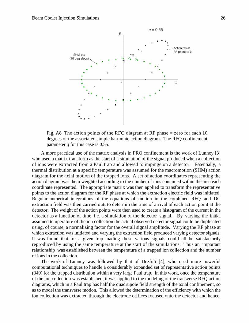
Fig. A8 The action points of the RFQ diagram at RF phase = zero for each 10degrees of the associated simple harmonic action diagram. The RFQ confinementparameter q for this case is 0.55.

A more practical use of the matrix analysis in FRQ confinement is the work of Lunney [3]who used a matrix transform as the start of a simulation of the signal produced when a collectionof ions were extracted from a Paul trap and allowed to impinge on a detector. Essentially, athermal distribution at a specific temperature was assumed for the macromotion (SHM) actiondiagram for the axial motion of the trapped ions. A set of action coordinates representing theaction diagram was them weighted according to the number of ions contained within the area eachcoordinate represented. The appropriate matrix was then applied to transform the representativepoints to the action diagram for the RF phase at which the extraction electric field was initiated.Regular numerical integrations of the equations of motion in the combined RFQ and DCextraction field was then carried outt to determin the time of arrival of each action point at thedetector. The weight of the action points were then used to create a histogram of the current in thedetector as a function of time, i.e. a simulation of the detector signal. By varying the initialassumed temperature of the ion collection the actual observed detector signal could be duplicatedusing, of course, a normalizing factor for the overall signal amplitude. Varying the RF phase atwhich extraction was initiated and varying the extraction field produced varying detector signals.It was found that for a given trap loading these various signals could all be satisfactorilyreproduced by using the same temperature at the start of the simulations. Thus an importantrelationship was established between the temperature of a trapped ion collection and the numberof ions in the collection.

The work of Lunney was followed by that of Dezfuli [4], who used more powerfulcomputational techniques to handle a considerably expanded set of representative action points(349) for the trapped distribution within a very large Paul trap. In this work, once the temperatureof the ion collection was established, it was applied to the modeling of the transverse RFQ actiondiagrams, which in a Paul trap has half the quadrupole field strength of the axial confinement, soas to model the transverse motion. This allowed the determination of the efficiency with which theion collection was extracted through the electrode orifices focused onto the detector and hence,


from an observation of the integrated signal current, a determination of the number of the ions inthe trap before extraction was initiated.

Kim [5] used matrix mechanics alone to numerically simulate the beam envelope of ionsextracted form RFQ ion guide. Again a specific temperature was assumed to set up the transverseaction diagrams of ions for different RF phases. The action ellipse for the displacement andmomentum of the sigmas of the disribution for that temperature (3) were then transported throughthe extraction region to the beam profile detector. The action ellipses for the different phases ofRF upon arrival there were compiled used the parameter εB of the individual sigma ellipses todetermine the gaussian radial distribution of the ion density each RF phase. The simulated overallbeam profile, which the detector of course averages over an RF cycle, was then compared with theobserved profile and the assumed temperature of the confined ions was adjusted until a match wasachieved. Fong [6] used a method very similar to that of Dezfuli to simulate the detector signal forions extracted from a linear RFQ ion trap.

References

[1] P. H. Dawson, “Quadrupole Mass Spectrometry and its Applications”, Elsevier ScientificPublications Co. (1976)

[2] RFQ_Action_movie

[3] M.D.N. Lunney, “The Phase Space Volume of Ion Clouds in a Paul Trap”, PhD Thesis,McGill University (1992)

[4] A.M.G. Dezfuli, “Injection, Cooling and Extraction of Ions from a Very Large Paul Trap”,PhD Thesis, McGill University (1996).

[5] T. Kim, “A Study of the Transmission of Ions Through RFQ Rods at High Buffer GasPressure”, PhD Thesis, McGill University (1998).

[6] C.W. Van Fong, Phase Space Dynamics in a Linear RFQ Trap for Time-of-Flight MassSpectrometry”, PhD Thesis, McGill Uniiversity (2001)


APPENDIX C - Units for ion motion calculations

Here I have to confess I am a closet SI unit abuser. While railing against those who push thecgs units of electromagnetism, without being able to convert from electric fields in those units toVolts per meter, I have been furtively steeling my ability to deal with off-the-wall questionsconcerning charged particle manipulations in electromagnetic traps by using a secret set of derivedunits of my own.

From the perspective of my present age I see that the addiction has its origins in a seminarattended many years ago on military ballistics, in which the speaker referred to the speeds ofexplosive waves and projectiles in pistols in millimeters per microsecond. When I asked him whyhe didn't say simply kilometers per second, he replied, as near as I can recall, "Bullets don't travelfor a second, particularly not inside a gun!".

In recent years I have spent a great deal of my time dealing with the manipulation of lowenergy charged particles, particularly in electromagnetic traps. After spending quite a few hourstracking down missing factors of 1.9 × 10-19, not to mention 2π, I became aware that using SIunits for such calculations was like expressing the distance to the supermarket in parsecs. Whatwas needed was a more reasonable unit, one on the scale of the particles that were being dealt with.It slowly dawned on me that the proper units were indeed the millimeter and the microsecond.

However, another unit was required to complete the basic set. The obvious selection of theamu as a unit of mass led to no great advantages. One still had to remember the electronic chargein these new units. Finally, with a perceptible tremor from all deceased high-school physicsteachers turning in their graves, I decided that the third basic unit had to be not of mass but offorce; specifically, Volts per millimeter.

Suddenly, as on the road from Tarsus, it all became clear. The derived unit of mass in thissystem becomes 96.48455 amu. (The derivation of this is left as an exercise to the reader.) Such aunit is just in the middle of the range of masses one deals with in low energy ion manipulations inmagnetic mass spectrometers, ion traps, time-of-flight spectrometers and ion mobility experiments.It is also close enough to 100 to make rough conversions of the ion mass from amu to these units,even with an overload of stimulating drink at a conference. Furthermore, it is obviously the naturalunit for ion manipulations since it results in the derived unit for magnetic field continuing to be theTesla.

I personally refer to this mass unit as the imu (ion mass unit). However, since my studentshave all discovered my addiction, though not all have succumbed to it, they have christened the unitthe "Mooron".

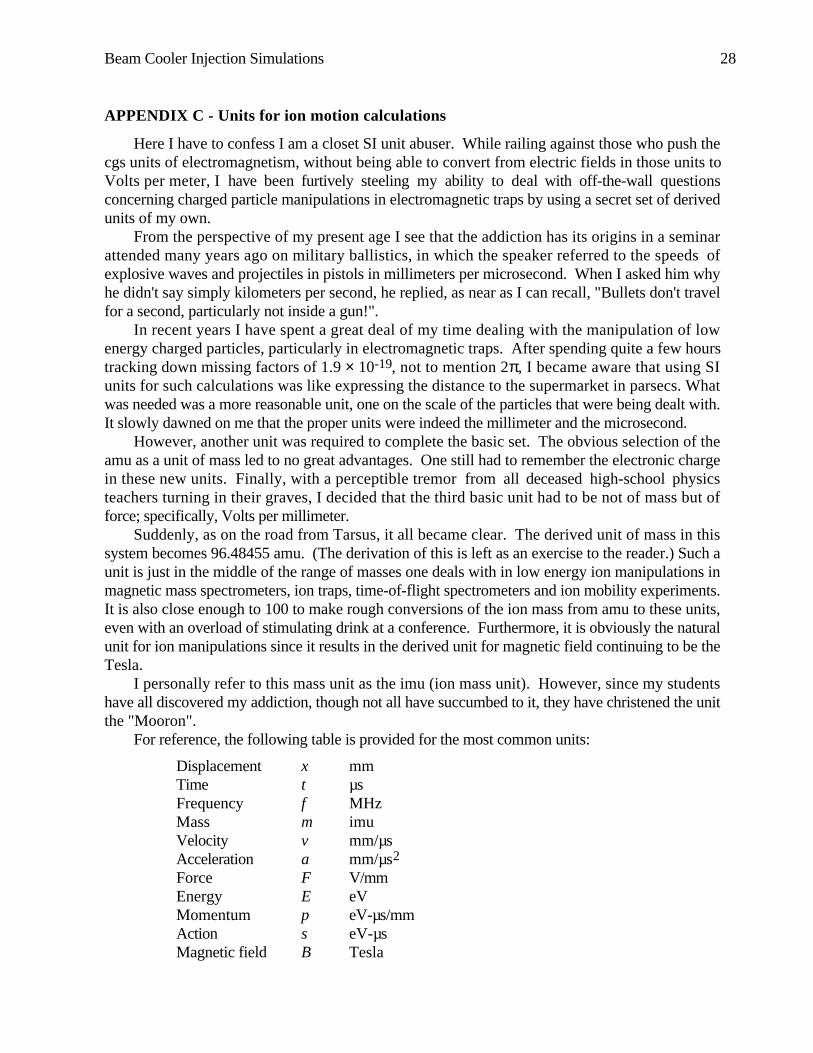
For reference, the following table is provided for the most common units:

Displacement x mmTime t µsFrequency f MHzMass m imuVelocity v mm/µsAcceleration a mm/µs2

Force F V/mmEnergy E eVMomentum p eV-µs/mmAction s eV-µsMagnetic field B Tesla


To convert to these units simply translate the ion mass into imu by dividing the atomic massby 96.5... The classical equations of elementary mechanics can then be applied.

F = max = 1/2 at2

p = mvs (action) = area of p-x diagramE = Fx = 1/2 mv2

Fmag = ϖ × B

In the unlikely event that relativistic mechanics must be applied, in imu the rest energy of anion is simply mc2. Taking the velocity of light as 3 × 105 mm/µs results in

Eo = mc2 = 9 × 1010 × m

A fringe benefit I have found from imu is that they enable me to translate the particlephysicist’s momentum unit of Mev/c to units used by mere mortals. I simply divide by 0.3 (i.e. c× 10-6).

Some Examples

Trajectory

An ion of mass 133 Daltons is traveling at 10000 m/s in an electric field of 300 Volts per cm.Its mass is 1.38 imu. Its velocity is 10 mm/µs. The force on it is 30 V/mm. Its initial momentum,energy and acceleration, and the distance it will travel in 3 µs are

E =

1

2mv2 =

1

2× 1.38 × 100 = 69 eV

p = mv = 1.38 × 10 = 13.8 eV-µs/mm

a =

F

m=

30

1.38= 21.74 mm/µs2

x = ut +

1

2at2 = 10 × 3 +

1

2× 21.74 × 9 = 128 mm

If the ion is initially traveling perpendicular to a magnetic field of 1.2 T, then the magneticforce on the ion is

FB = vB = 10 × 1.2 = 12 V/mm

The magnetic rigidity of the particle, in T-mm, is the momentum in eV-µs/mm. The initial radiusof curvature of the particle trajectory is therefore

ρ =

(Bρ)

B=

13.8

1.2= 11.5 mm


Trap

If the electric field in a trap forms a simple harmonic potential well given by

F = kx ; k - V/mm2,

then the frequency of the simple harmonic motion of an ion, in radians per µs, is

ω =

k

m

If the trap has a potential well depth of 10 V over a span of ± 5 mm, then

k = 0.8 V/mm2

and an ion of mass 133 Daltons will have a radian oscillation frequency of

ω =

0.8

1.38 = 0.76 rad- µs -1 .

rfq beam cooler injection simulation - mcgill …moore/notes/rfq_injection.pdf · rfq beam cooler...

Documents