rfxphqw 9huvlrq /lqn wr wkh ilqdo sxeolvkhg...

Final published version

https://academic.oup.com/mnras/article/478/3/4010/5026631 This article has been published in Monthly Notices of the Royal Astronomical Society © 2018 The Author(s). Published by Oxford University Press on behalf of the Royal Astronomical Society. All rights reserved.

Vries, M. N. D., Wise, M. W., Huppenkothen, D., Nulsen, P. E. J., Snios, B., Hardcastle, M. J., ... McNamara, B. R. (2018). Detection of non-thermal X-ray emission in the lobes and jets of Cygnus A. Monthly Notices of the Royal Astronomical Society. DOI: 10.1093/mnras/sty1232

MNRAS 478, 4010–4029 (2018) doi:10.1093/mnras/sty1232Advance Access publication 2018 June 1

Detection of non-thermal X-ray emission in the lobes and jets of Cygnus A

M. N. de Vries,1‹ M. W. Wise,1,2‹ D. Huppenkothen,3 P. E. J. Nulsen,4‹ B. Snios,4

M. J. Hardcastle,5 M. Birkinshaw,6 D. M. Worrall,6 R. T. Duffy6 and B. R. McNamara7,8

1Astronomical Institute ‘Anton Pannekoek’, University of Amsterdam, Science Park 904, NL-1098 XH Amsterdam, the Netherlands2ASTRON, Netherlands Institute for Radio Astronomy, Postbus 2, NL-7990 AA Dwingeloo, the Netherlands3Department of Astronomy, University of Washington, 3910 15th Ave NE, Seattle, WA 98195, USA4Harvard-Smithsonian Center for Astrophysics, 60 Garden Street, Cambridge, MA 02138, USA5School of Physics, Astronomy and Mathematics, University of Hertfordshire, College Lane, Hatfield AL10 9AB, UK6HH Wills Physics Laboratory, University of Bristol, Tyndall Avenue, Bristol BS8 1TL, UK7Department of Physics and Astronomy, University of Waterloo, 200 University Ave W, Waterloo, ON N2L 3G1, Canada8Perimeter Institute for Theoretical Physics, 31 Caroline St North, Waterloo, ON N2L 2Y5, Canada

Accepted 2018 May 4. Received 2018 May 4; in original form 2018 January 19

ABSTRACTWe present a spectral analysis of the lobes and X-ray jets of Cygnus A, using more than 2 Msof Chandra observations. The X-ray jets are misaligned with the radio jets and significantlywider. We detect non-thermal emission components in both lobes and jets. For the eastern lobeand jet, we find 1 keV flux densities of 71+10

−10 and 24+4−4 nJy, and photon indices of 1.72+0.03

−0.03

and 1.64+0.04−0.04, respectively. For the western lobe and jet, we find flux densities of 50+12

−13 and13+5

−5 nJy, and photon indices of 1.97+0.23−0.10 and 1.86+0.18

−0.12, respectively. Using these results, wemodelled the electron energy distributions of the lobes as broken power laws with age breaks.We find that a significant population of non-radiating particles is required to account for thetotal pressure of the eastern lobe. In the western lobe, no such population is required andthe low energy cutoff to the electron distribution there needs to be raised to obtain pressuresconsistent with observations. This discrepancy is a consequence of the differing X-ray photonindices, which may indicate that the turnover in the inverse-Compton (IC) spectrum of thewestern lobe is at lower energies than in the eastern lobe. We modelled the emission fromboth jets as IC emission. There is a narrow region of parameter space for which the X-ray jetcan be a relic of an earlier active phase, although lack of knowledge about the jet’s electrondistribution and particle content makes the modelling uncertain.

Key words: galaxies: individual: Cygnus A – galaxies: jets – X-rays: galaxies.

1 IN T RO D U C T I O N

Cygnus A (hereafter Cyg A) is an FRII radio galaxy (Fanaroff &Riley 1974). Its extreme radio brightness (Stockton & Ridgway1996) made it one of the first objects of such type to be discovered.Radio observations show extended, plume-like lobe structures ofsynchrotron-emitting plasma, as well as jets extending to the eastand west of the AGN, which terminate in bright hotspots wherethe jets are driving shocks into the surrounding intracluster medium(ICM) (Carilli, Perley & Dreher 1988; Carilli et al. 1991; Carilli,Perley & Harris 1994). In the X-ray, these shocks are observed asa sharp brightness edge ahead of the hotspots, and are also referredto as the cocoon shocks (Wilson, Smith & Young 2006).

Inverse-Compton (IC) emission has been detected in the lobesand hotspots of many FRII sources, (e.g Hardcastle et al. 2002;

� E-mail: [email protected] (MdV); [email protected] (MW);[email protected] (PN)

Konar et al. 2009). There are different names for the IC emissiondepending on the seed photons that are scattered. The types usuallyconsidered are IC scattering of the cosmic microwave background(IC/CMB) (Harris & Grindlay 1979), of synchrotron photons (syn-chrotron self-Compton, or SSC), or of infrared photons from theAGN (Brunetti, Setti & Comastri 1997). Because the IC spectrumis directly linked to the electron energy distribution, it probes low-energy electrons in the lobes. The combination of the X-ray ICspectrum, the radio synchrotron spectrum and the total pressurethen provide constraints on the distribution of electron energiesand the magnetic field strength in the lobes. For FRII sources ithas been shown that most sources have overpressured lobes withelectron-dominated internal energies (Ineson et al. 2017).

It is common to assume equipartition to model the lobe en-ergy density, especially for FRI galaxies. Many FRI galaxies showdeficits compared to the external pressure that seem to requirea significant quantity of non-radiating particles, such as protons(Morganti et al. 1988; Bırzan, Rafferty & McNamara 2004; Hard-

C© 2018 The Author(s)Published by Oxford University Press on behalf of the Royal Astronomical Society

Downloaded from https://academic.oup.com/mnras/article-abstract/478/3/4010/5026631by University of Hertfordshire useron 26 July 2018

mailto:[email protected]



Non-thermal X-ray emission in Cyg A 4011

castle et al. 2007). This population could be created by entrainmentof material by the jets (Croston et al. 2008; Croston & Hardcastle2014).

Detecting IC emission from the lobes in Cyg A has proven chal-lenging as a result of the rich cluster environment containing bright,relatively hot thermal emission. Recent work by Wise et al. (inpreparation) shows that the ICM around and in front of the west-ern lobe is significantly hotter than on the eastern side, and showsmore temperature variation. This temperature structure could be asignature of earlier cycles of AGN activity, a shock generated bythe early phase merger with the northwestern subcluster (CygnusNW), or some combination of the two.

Previous work has claimed detection of non-thermal emissionin the Cyg A lobes (Hardcastle & Croston 2010; Yaji et al. 2010).The non-thermal lobe fluxes in these papers are consistent with eachother, although the errors are large. The result shows that Cyg A maybe different from other FRII galaxies in that the electron populationis not energetically dominant, and that the jet entrainment model forFRI radio galaxies may be important for Cyg A as well (Hardcastle& Croston 2010).

The wide, linear features extending east and west of the AGN inthe X-ray are generally assumed to be X-ray analogues of the radiojets. Although the nature of these features is partially unclear, wewill refer to them throughout this paper as the X-ray jets. Dreher,Carilli & Perley (1987) derived an upper limit to the thermal electrondensity in the lobes of Cyg A, using Faraday rotation measurements.These limits are difficult to reconcile with a thermal model for thejet emission, as shown in Steenbrugge, Blundell & Duffy (2008).

If the X-ray jets are non-thermal in origin, it is unclear whichnon-thermal emission mechanism would produce extended X-rayjets on kiloparsec scales. Generally, two different models have beeninvoked for these kinds of jets. The first model is the boostedIC/CMB model (Tavecchio et al. 2000; Celotti, Ghisellini & Chi-aberge 2001). In this model, high bulk Lorentz factors at smallangles to the line-of-sight Doppler boost the upscattered photonsenough to produce detectable X-ray emission. The model has beenapplied to quasar jets. However, in Cyg A the eastern, receding jetappears to be brighter in X-rays than the western, approaching jet.Doppler boosting would only have the opposite effect on the east-ern jet, and increase the difference in intrinsic emissivities betweenthe two jets. Therefore, we consider the boosted IC/CMB modelunlikely to apply to Cyg A.

The synchrotron model is often proposed as an alternative tothe IC/CMB model. X-ray synchrotron emission requires elec-trons with very high Lorentz factors. Because the lifetime of X-raysynchrotron-emitting electrons is only of the order of tens to hun-dreds of years, the electrons require in situ acceleration. Electronre-acceleration is achieved through shocks, which happen locallyin jet knots. A synchrotron jet model can therefore explain morenaturally the knottiness seen in some of the extended X-ray jets(Hardcastle et al. 2016). In synchrotron models, many systems withmultiwavelength observations show that the radio, optical/IR, andX-ray data cannot be explained with a single electron energy dis-tribution, which implies the existence of a second, more energeticcomponent (e.g. Hardcastle 2006; Jester et al. 2006; Uchiyama et al.2006). It is unclear how a second electron energy distribution couldbe created.

A few morphological differences make the Cyg A jets unlike mostother radio/X-ray jet systems. The most obvious difference is thatthe X-ray jets are at least 4–6times wider than the radio jet, extend-ing several arcseconds in width. An extended X-ray jet structure hasbeen observed in the quasar PKS 1055+201 (Schwartz et al. 2006).

Moreover, the X-ray jets and radio jets are misaligned (Steenbrugge& Blundell 2008). While aligned with each other close to the AGN,midway to the lobe the X-ray jets extend relatively straight towardsthe brightest hotspots, while the radio jets bend southwards to thefainter hotspots. Based on these morphological differences, Steen-brugge et al. (2008) argue that the Cyg A jets are IC/CMB-emittingrelic jets, emitted by an older electron population that was left be-hind from earlier passage of the radio jet. In this model, when theradio jet changes direction through precession or for some other rea-son, the electron population of the radio jet expands adiabaticallyinto the medium, reducing electron energies to the range required toproduce IC/CMB X-rays. This would explain the spatial misalign-ment of the jets, as well as the greater width of the X-ray jet. The ICrelic jet model could also explain the brightness difference betweenthe two jets through the difference in light travel time. The CygA cocoon is inclined at ∼55 deg to our line of sight (Vestergaard& Barthel 1993). This means light from the eastern hotspot has anadditional light travel time of ∼2 × 105 yr. The difference in lighttravel time could explain the relative faintness of the western jet: ithas had more time to fade and expand.

However, the question remains how this relic X-ray jet couldexist long enough as a linear feature for us to observe it. If theadiabatic expansion is too fast, the jets would not be observed as alinear feature. Moreover, a fast expansion of the jet would shock thematerial in the lobes. The observed X-ray jet morphology impliesthat the jets would have to be fairly close to pressure balance with thelobes. Because the jets are brighter than the surrounding lobe, thisis difficult to achieve unless the jets and lobes have significantlydifferent electron populations or particle content. Additionally, itis difficult to maintain the observed knotty jet structure as thisimplies significant local pressure variations. In an expanding relicjet scenario, those pressure variations should smooth out during theexpansion.

In this paper, we use 1.8 Ms of new Chandra observations, com-bined with 200 ks of archival observations, to analyse the emissionfrom the lobes and X-ray jets of Cyg A. Complementary results forthe inner gas structure and outer lobe shocks appear in Duffy et al.(2018) and Snios et al. (2018), respectively. We compare differentmodels for the lobe and jet emission and constrain their parameters.With these parameters, we model the energy density of the lobesand test the possibility of an IC relic jet. We show the data anddetail the data reduction in Section 2. We give an overview of thestatistical tools and the models that we used in Section 3. We presentthe results of the statistical analysis in Section 4, and discuss theirinterpretation in Section 5. We conclude in Section 6.

Throughout this paper, we adopt a cosmology with H0= 69.3 kms−1 Mpc−1, �M = 0.288, and �� = 0.712 (Hinshaw et al. 2013).We use a redshift value of z = 0.0561 (Stockton, Ridgway & Lilly1994). This yields a linear scale of 66 kpc arcmin−1 and a luminositydistance DL = 253.2 Mpc for Cyg A. The spectral index α isdefined so that flux ∝ ν−α , and related to the X-ray photon index as� = 1 + α.

2 X - R AY O B S E RVAT I O N S A N D DATAR E D U C T I O N

2.1 Data reduction

This paper uses nearly all of the Cyg A data available on the Chan-dra archive. This includes 200 ks of previous observations takenbetween 2000 and 2005, and 2 Ms of recent observations takenbetween 2015 and 2017. A subset of 200 ks of the recent ob-

MNRAS 478, 4010–4029 (2018)Downloaded from https://academic.oup.com/mnras/article-abstract/478/3/4010/5026631by University of Hertfordshire useron 26 July 2018

4012 M. N. de Vries et al.

servations were excluded, as they are pointed at the northwesternsubcluster Cyg NW and the filamentary region between the twosubclusters. This leaves a total data set of more than 2 Ms. A logof all the observations, with their filtered exposure times and point-ings, is shown in Table 1. For an extended review of the full data setand the large-scale structure of the system, we refer to Wise et al.(in preparation).

Each of these data sets has been reprocessed with CIAO 4.9 andCALDB 4.7.4 (Fruscione et al. 2006). Before reprocessing the data, wecorrected for small astrometric errors caused by Chandra’s pointingaccuracy of around 0.5 arcsec. We followed the procedure describedby Snios et al. (2018), briefly summarized here. We chose ObsID5831 as the reference observation for the high total counts. We thenreprojected the event lists of the other ObsID onto the sky frame ofObsID 5831. For each ObsID, we cross-correlated a 0.5–7.0 keV160 x 120 arcsec region around the central AGN with ObsID 5831to determine the coordinate offset. The coordinate shift was thenapplied to the event list and aspect solution files with wcs update.

After the astrometry correction, we applied the following CIAO

processing tools. For each ObsID, a new badpix file was built withacis build badpix. We applied the latest gain and CTI correctionswith acis process events. We created a new level 2 event file byfiltering for good grades (0, 2, 3, 4, 6). After that, we filtered forGTIs with the tool deflare. Finally, we identified readout streakswith acis streak map and filtered them out.

The background event files were created from the ACIS blanksky event files. The backgrounds were imported from the calibra-tion database with the tool acis bkgrnd lookup, and reprojected.The backgrounds were scaled to the data by using the counts be-tween 10.0 and 12.0keV. The event files and backgrounds were allseparately reprojected and added together to form a merged countsimage and a merged background map. We show the merged 0.5–7.0 keV counts image in Fig. 1.

As well as the X-ray data, we have used two radio maps of thesystem: a 4.5 GHz VLA radio map from Perley, Dreher & Cowan(1984), and 150 MHz LOFAR radio map from McKean et al. (2016).The radio maps were used to define the extent of the lobe extractionregions on the X-ray data. We also used the radio fluxes within theseregions to do combined modelling of the radio and X-ray spectra.No additional processing has been done to the radio data.

In the Chandra image, we observe a brightness edge in the easternlobe just above the northern hotspot that corresponds with the edgeof the lobe in the VLA data. This is empirical evidence that we aredirectly observing the non-thermal emission from the lobe in theX-ray data in this region. We have indicated this region with a blackarrow in Fig. 1.

2.2 Extraction regions and spectra

We used the CIAO fitting package SHERPA (Freeman, Doe & Siemigi-nowska 2001) to analyse the spectra. All spectral models men-tioned in this paper are multiplied by a PHABS foreground Galac-tic absorption model. The Galactic HI column density is set at3.1 × 1021 atoms cm−2. This value is based on the average of thecolumn densities of the Leiden/Argentine/Bonn (LAB) and Dickey& Lockman surveys (Dickey & Lockman 1990; Kalberla et al.2005). The thermal model used in this paper is the AstrophysicalPlasma Emission Code (APEC; Smith et al. 2001), with the elementalabundance model from Anders & Grevesse (1989).

To better highlight the wealth of structure within the Cyg Acocoon shock, we created a residual map of the data. This wasdone by subtracting a radial unsharp masked image (Wise et al. in

preparation). This technique is similar to traditional unsharp mask-ing techniques. A radon transform was applied to the background-subtracted, merged image of the core. Each column of pixels wasthen smoothed with a 7 arcsec 1D Gaussian kernel. The smoothedimage was transformed back to Cartesian coordinates and subtractedfrom the input image. The resulting residual map, together with theextraction regions, are shown in Fig. 2. The radial unsharp maskingtechnique has the advantage that it only smooths in the radial direc-tion. Therefore, there is less risk of creating artefacts by mismatchedGaussian smoothing kernels.

We assume that the X-ray jets are tube-like structures in-side the lobes, which are in turn embedded in a shell of ther-mal ICM. With this geometry in mind, we define three differenttypes of extraction regions: the X-ray jet regions (J), lobe re-gions (L), and thermal background regions (B). For each lobe,we defined three sets of J, L, and B regions, which allows forvariation in the thermal properties of the ICM along the jet axis.The X-ray jet regions were made to trace the jet as seen on theresidual map. In the eastern lobe especially, the jet makes a notice-able bend which the extraction regions follow. The width of eachjet region was set to be the FWHM of the surface brightness peakperpendicular to the jet in that region. This definition results in vari-ations in the width of the jet extraction regions along the jet path.In defining the edges of the lobe, we have taken care to include theregions with the brightest lobe emission that lie within the cocoonshock. We have therefore opted to use the VLA map rather thanthe LOFAR map, as electrons that produce synchrotron emission at150 MHz, will IC scatter those synchrotron photons to energies be-low 1 eV. Because SSC emission is considered to strongly contributeto the total IC flux, we expect regions that show only low-frequencyradio emission to show less non-thermal X-ray emission.

We determined the noise level on the VLA 4.5 GHz continuummap to be 0.8 mJy beam−1. We then defined contours around thelobe at the 5σ level, or 4 mJy beam−1, at a smoothing scale of 20pixels. These contours enclose the brightest lobe emission. The loberegions on each side were then defined as ellipses approximatelyfollowing these contours. We trimmed the lobe regions close tothe hotspots, as we expect the cocoon shock emission to domi-nate here over any possible non-thermal emission from the X-rayjet and lobes. In the western lobe, the ellipse was trimmed on thesouthern side to follow the asymmetric shape of the radio lobe.Finally, the thermal background regions were created by draw-ing ellipses around the lobe regions on each side. These regionswere defined close to the lobes so that their thermal proper-ties do not differ much from the thermal properties of the ma-terial in front of the lobes. The outer edge of the radio lobedoes enter slightly into the thermal background regions in theouter parts, although the radio lobe drops off in flux sharply be-yond the defined lobe size. The thermal spectra for the back-ground regions are not subtracted from the spectra, but rathertheir temperatures and abundances are used to constrain thermalemission from material superposed on the lobe and jet regions.Using specextract, we extracted the events within each extractionregion from every ACIS chip that overlaps with that region. We ob-tained source spectra, response files, and blank sky spectra for eachregion on each ACIS chip of each observation. After the extraction,we combined the spectra of for all ACIS-S and ACIS-I observationswith combine spectra. This results in one combined spectrum, set ofresponse files, and blank sky background spectrum for each region.We have used these combined spectra in the rest of the analysis.combine spectra automatically adds all the exposure times of in-dividual spectra together when combining. However, this means



Table 1. Observation log of Chandra Cyg A data used in this paper.

ObsIDa Dateb Texpc (ks) Pointingd ObsIDa Dateb Texp

c (ks) Pointingd

360∗ 2000 05 21 34.7 Nucleus 17138 2016 07 25 26.4 W Hotspot1707∗ 2000 05 26 9.2 Nucleus 17513 2016 08 15 49.1 Nucleus6225 2005 02 15 24.3 Nucleus 17516 2016 08 18 49.0 W Hotspot5831 2005 02 16 50.8 Nucleus 17523 2016 08 31 49.4 E Hotspot6226 2005 02 19 23.7 Nucleus 17512 2016 09 15 66.9 Nucleus6250 2005 02 21 7.0 Nucleus 17139 2016 09 16 39.5 W Hotspot5830 2005 02 22 23.2 Nucleus 17517 2016 09 17 26.7 W Hotspot6229 2005 02 23 22.8 Nucleus 19888 2016 10 01 19.5 W Hotspot6228 2005 02 25 16.0 Nucleus 17140 2016 10 02 34.3 W Hotspot6252 2005 09 07 29.7 Nucleus 17507 2016 11 12 32.4 Nucleus17530 2015 04 19 21.3 E Hotspot 17520 2016 12 06 26.8 W Hotspot17650 2015 04 22 28.2 E Hotspot 19956 2016 12 10 54.1 W Hotspot17144 2015 05 03 49.4 E Hotspot 17514 2016 12 13 49.4 Nucleus17141 2015 08 01 29.6 E Hotspot 17529 2016 12 15 35.1 E Hotspot17710 2015 08 07 19.8 E Hotspot 17519 2016 12 19 29.4 W Hotspot17528 2015 08 30 49.3 E Hotspot 17135 2017 01 20 19.8 Nucleus17143 2015 09 03 27.1 E Hotspot 17136 2017 01 26 22.2 Nucleus17524 2015 09 08 23.0 E Hotspot 19996 2017 01 28 28.6 Nucleus18441 2015 09 14 24.6 E Hotspot 19989 2017 02 12 41.5 Nucleus17526 2015 09 20 49.4 E Hotspot 17515 2017 03 22 39.0 W Hotspot17527 2015 10 11 26.8 E Hotspot 20043 2017 03 26 29.3 W Hotspot18682 2015 10 14 22.8 E Hotspot 20044 2017 03 27 14.6 W Hotspot18641 2015 10 15 22.4 E Hotspot 17137 2017 03 30 25.2 W Hotspot18683 2015 10 18 15.6 E Hotspot 17522 2017 04 08 48.6 W Hotspot17508 2015 10 28 14.9 Nucleus 20059 2017 04 19 23.7 E Hotspot18688 2015 11 01 34.6 Nucleus 17142 2017 04 20 23.3 E Hotspot18871 2016 06 13 21.8 Nucleus 17525 2017 04 22 24.7 E Hotspot17133 2016 06 18 30.2 Nucleus 20063 2017 04 22 25.4 E Hotspot17510 2016 06 26 37.3 Nucleus 17511 2017 05 10 15.9 Nucleus17509 2016 07 10 51.2 Nucleus 20077 2017 05 13 27.7 Nucleus17518 2016 07 16 49.4 W Hotspot 20048 2017 05 19 22.7 E Hotspot17521 2016 07 20 24.5 W Hotspot 17134 2017 05 20 29.4 Nucleus18886 2016 07 23 21.5 W Hotspot 20079 2017 05 21 23.8 Nucleus

Total 2005.3

aThe Chandra Observation ID number. ObsID’s marked with an asterisk indicate ACIS-S observations.bThe date of the observation .cThe exposure times after filtering for flares.dThe aimpoint location of the observation. Three different aimpoints have been used in this data set: the AGN,as well as the western and eastern hotspots.

Figure 1. The merged 0.5–7.0 keV counts image Cyg A, binned withnative 0.492 arcsec pixels. The black arrow indicates a brightness edgecorresponding to the lobe edge. See the text for details.

that when an extraction region falls on two different chips withinthe same ObsID, the exposure time of that ObsID is erroneously

counted twice. We therefore re-calculated the exposure time of eachspectrum manually after the combining process. We have chosento combine both the ACIS-I and ACIS-S spectra together into onecombined spectrum for each region. This was done because theACIS-S data only makes up 45 ks of the total 2 Ms exposure time.Furthermore, the ∼5−8keV temperature of the gas around Cyg Ais sufficiently high that the response below 2 keV, where ACIS-Sand ACIS-I are most different, is unlikely to drive the fit results.To test this, we created combined spectra for regions B2 and B4that only include ACIS-I observations. We then compared the totalcombined spectra to the ACIS-I combined spectra. In both regions,the difference in temperature and abundance are less than 1 per cent.

In the eastern lobe and jet, the combined spectra contain an av-erage of ∼70 000 and ∼25 000 counts per region, respectively. Inthe western lobe and jet, the combined spectra contain an averageof ∼36 000 and ∼14 000 counts per region, respectively. Despitethe high number of counts in each region, it is difficult to disen-tangle thermal from non-thermal models at CCD resolution withstandard fitting procedures. To illustrate this, we took the spec-trum of lobe region L2 and subtracted the blank sky backgroundfor the same region. We then fit two models to this spectrum: a



Figure 2. Radial unsharp masked residual image of the Cyg A core. Shown in green are smoothed contours of the 4.5 GHz VLA radio data. Shown in whiteare the jet (J), lobe (L), and background (B) extraction regions. The schematic illustrations next to each lobe indicate how the regions are labelled.

thermal APEC model, or a combination of thermal and non-thermalemission (APEC + POWERLAW). The resulting fits are shown inFig. 3. An APEC fit gives a χ2/dof of 433/430, while the APEC+ POWERLAW fit gives a χ2/dof of 433/428. Because the power-law component is weak compared to the thermal component, thedifference in the parameters between models is small: the APEC

model gives T = 6.36 ± 0.09 keV and Z = 0.42 ± 0.03, whilethe APEC + POWERLAW model gives T = 6.48 ± 0.18 keV andZ = 0.44 ± 0.03, and � = 2.06 ± 0.62. This example illustrates thatwhen a non-thermal emission component is included in the model,the fit is not significantly improved, and that because of its smallamplitude compared to the thermal component, it does not have asignificant effect on the thermal parameters. Therefore, statisticaltests such as an F-test do not give convincing evidence for or againstthe presence of power-law emission.

Instead, of treating each region separately, we will treat all theregions in each jet and lobe together. By building a Bayesian modelfor each lobe and jet, we can simultaneously fit regions while settingpriors for each of the parameters in our model. It also allows us toMCMC sample the models and thereby obtain posterior distribu-tions for each parameter. We describe the statistical approach andthe models used in the next section.

3 STATISTICAL ANALYSIS

3.1 Statistical approach

We give a brief overview of the statistical approach here. For a moreextended review of Bayesian inference, Markov Chain Monte Carlo(MCMC) sampling, and model comparison, we refer to Appendix A.The models are described in more detail in Section 3.2.

We defined two competing models for the lobe regions on eachside: one model with only thermal emission and one which includesboth thermal and non-thermal emission. For each of these models,we determined the maximum loglikelihood through a Maximum APosteriori (MAP) estimate. Each model was also sampled with anMCMC algorithm. We used the PYTHON module EMCEE (Foreman-Mackey et al. 2013), which implements an affine invariant ensembleMCMC sampler based on Goodman & Weare (2010).

The likelihoods obtained from the MAP estimate were used tocompare the models with the corrected Akaike Information Cri-terion (AICC) and the Bayesian Information Criterion (BIC). Wehave used the likelihood ratio test (LRT) as an additional modelcomparison tool. The LRT is a form of hypothesis testing for thelikelihood ratio between two nested models. The MCMC sampleddata of the thermal model were used for the LRT, to generate fakedata under the null hypothesis. We then applied a MAP for bothmodels to this data, and compared the likelihood ratio to the likeli-hood ratio of the real data. With the help of these model comparisontests, we selected the most likely model and used the posterior dis-tributions obtained from the MCMC sampling in the rest of theanalysis.

We defined two competing models for the X-ray jet regions oneach side as well: one thermal model and one non-thermal model.Because the jets are embedded in the lobes, the jet model needsto include all the terms from the lobe model. We used the poste-rior distributions from the lobe models, obtained through MCMCsampling, to set priors on the lobe components in the jet regions.As in the lobes, we determined the maximum loglikelihood of thetwo competing models through a MAP estimate and used AICC

and BIC to compare the models and select the most likely model.The LRT is only valid for nested models and could therefore notbe used here. The most likely model was MCMC sampled and



Figure 3. Comparison of two different models, both fit to the spectrum ofregion L2. The top image shows an APEC model, the bottom image an APEC+ POWERLAW model.

the resulting posterior distributions were used in the rest of thisanalysis.

Throughout this paper, when values from the posterior distribu-tions are quoted, we have used the median together with the 14thand 86th percentile as lower and upper errors, respectively. If thedata are distributed as a Gaussian, this would correspond to a 1σ

credibility interval. Because the posterior distribution is not neces-sarily Gaussian in shape, we also show the posterior distributionsthat result from the MCMC sampling.

3.2 Model description

3.2.1 Source models

The lobes and X-ray jets were analysed sequentially, so that we canapply model comparison tests first to the lobes and then to the jets.The background regions are not included in the model itself. Instead,they are fit in SHERPA with an APEC model, and the temperatures andabundances from these regions are used as priors for the thermalcomponents in the lobe and jet models, as described in more detailin Section 3.2.2. Because the definition of the edge of the lobeis somewhat arbitrary, we cannot rule out that some non-thermalemission is present in the background regions as well. However, as

we have already seen in the fit comparison in Section 2.2, addinga non-thermal component to the model affects the temperature andabundance very little, even in a region that is in the middle of thelobe. Therefore, the error in our assumption will likely be smallerthan the width of the prior.

Each spectrum is fitted between 0.5 and 7.0 keV. In the loberegions, we compare two different models. In model ML0, every re-gion contains a thermal model. The alternative model, ML1 containsthe same thermal model, with a power law added to describe thenon-thermal emission. The models are nested, such that ML1 = ML0

when the amplitude of the power law is zero. Lobe models ML0 andML1 are described in Table 2. We give a detailed description on thepriors of the model in Section 3.2.2.

Because we assume that the jets are embedded in the lobes, thejet model consists of lobe model ML with an additional componentto describe the jet. Whether the background is the thermal modelML0 or the model with non-thermal emission ML1 is determined inthe model selection between ML0 and ML1. The jet itself is modelledeither as a second thermal component with the same abundance andtemperature across the jet, MJ0, or a second power law with the samephoton index across the jet, MJ1. The jet models MJ0 and MJ1 aredescribed in Table 3. The jet models, in contrast to the lobe models,are not nested. This means that we can apply the information criteriabut not the LRT.

We note that Tables 2 and 3 show the parameters for just one set oflobe and jet regions. As indicated in the table, most parameters aredifferent for each lobe and jet region. However, we have constrainedthe photon index �1 and the parameters σ L and σ J only have onevalue throughout the lobe. In the jet models, we assume either asingle temperature and abundance (MJ0), or a single photon index�2 (MJ1) throughout the entire jet.

3.2.2 Priors

From MCMC sampling of the lobe models we obtain posterior dis-tributions of each parameter in the model. We subsequently usethese posterior distributions as priors for the jet model. The proba-bility distributions are obtained by making a one-dimensional kerneldensity estimation (KDE) over the posterior distribution of each pa-rameter. We have used an asymmetric KDE so that the smoothingeffect close to the prior boundaries is minimized. This is a particularconcern for some of the normalization parameters, where most ofthe posterior distribution could lie close to the prior boundary atzero.

We make the assumption that any thermal or non-thermal modelcomponent in a given lobe region has the same surface bright-ness as that same component in the corresponding jet region. Thisallows us to take the posterior distributions of the thermal or non-thermal normalization in a lobe region, scale them by area anduse them as prior distributions for the jet region. Because the jetmodels either contain two different thermal or non-thermal modelcomponents, setting a prior on one of them makes it easier to dis-tinguish between these two components. The assumption that thesurface brightness of a component is the same in the middle ofthe lobe (where the X-ray jet is) as on the side, is unlikely tobe completely accurate. However, assuming anything about thethree-dimensional geometry of the lobe and the jet would intro-duce additional uncertainties as well. Furthermore, the error in thisassumption will likely be subsumed in the width of the input priordistribution.



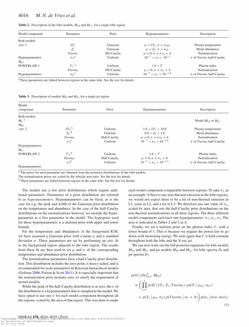
Table 2. Description of the lobe models, ML0 and ML1, for a single lobe region.

Model component Parameter Prior Hyperparameters Description

Both modelsAPEC 1 kT1 Gaussian μ = kT1, σ = σ kT1 Plasma temperature

Z1 Gaussian μ = Z1, σ = σ Z1 Metal abundanceTnorm1 Hlf-Cauchy μ = 0, σ = σ T1 × A Normalization

Hyperparameters σ Ta Uniform 10−7 < σ T < 10−3 σ of Tnorm1 half-Cauchy

ML1

POWERLAW 1 �1a Uniform 1.0 < � Photon index

Pnorm1 Hlf-Cauchy μ = 0, σ = σ L × A NormalizationHyperparameters σ L

a Uniform 10−7 < σ L < 10−3 b σ of Pnorm1 half-Cauchy

aThese parameters are linked between regions in the same lobe. See the text for details.

Table 3. Description of models MJ0 and MJ1, for a single jet region.

Modelcomponent Parameter Prior Hyperparameters Description

Both modelsML

a Model ML0 or ML1

MJ0

APEC 2 kT2b Uniform 1.0 < kT2 < 10.0 Plasma temperature

Z2b Uniform 0.0 < Z2 < 1.0 Metal abundance

Tnorm2 Half-Cauchy μ = 0, σ = σ T2 × A Normalization

Hyperparametersσ J

a Uniform 10−7 < σ J < 10−3 b σ of Tnorm2 half-Cauchy

MJ1

POWERLAW 2 �2b Uniform 1.0 < � Photon index

Pnorm2 Half-Cauchy μ = 0, σ = σ J × A Normalization

Hyperparametersσ J

b Uniform 10−7 < σ L < 10−3 b σ of Pnorm2 half-Cauchy

a The priors for each parameter are obtained from the posterior distributions of the lobe models.The normalization priors are scaled by the lobe/jet area ratio. See the text for details.b These parameters are linked between regions in the same lobe. See the text for details.

The models use a few prior distributions which require addi-tional parameters. Parameters of a prior distribution are referredto as hyperparameters. Hyperparameters can be fixed, as is thecase for e.g. the peak and width of the Gaussian prior distributionon the temperature and abundance. In the case of the half-Cauchydistributions on the normalizations however, we include the hyper-parameter as a free parameter in the model. The hyperprior usedfor those hyperparameters is a uniform prior with upper and lowerbounds.

For the temperature and abundances of the foreground ICM,we have assumed a Gaussian prior with a mean μ and a standarddeviation σ . These parameters are set by performing an APEC fitto the background region adjacent to the lobe region. The resultsfrom these fit are then used to set μ and σ of the correspondingtemperature and abundance prior distribution.

The normalization parameters have a half-Cauchy prior distribu-tion. This distribution includes the zero point, is heavy-tailed, and isrecommended for scale parameters in Bayesian hierarchical models(Gelman 2006; Polson & Scott 2011). It is especially important thatthe normalization prior includes zero, to satisfy the requirement ofnested models.

While the peak of the half-Cauchy distribution is at zero, the σ ofthe distribution is a hyperparameter that is sampled in the model. Wehave opted to use one σ for each model component throughout allthe regions, scaled by the area of that region. This was done to make

each model component comparable between regions. To take σ L asan example: if there is any non-thermal emission in the lobe regions,we would not expect there to be a lot of non-thermal emission inL1, none in L2, and a lot in L3. We therefore use one value of σ L,scaled by area, that sets the half-Cauchy prior distributions on thenon-thermal normalizations in all three regions. The three differentmodel components each have one hyperparameter: σ T, σ L, σ T. Thearea is indicated in Tables 2 and 3 as A.

Finally, we set a uniform prior on the photon index �, with alower bound of 1. This is because we require the power law to godown with increasing energy. We note again that � is held constantthroughout both the lobe and the X-ray jet.

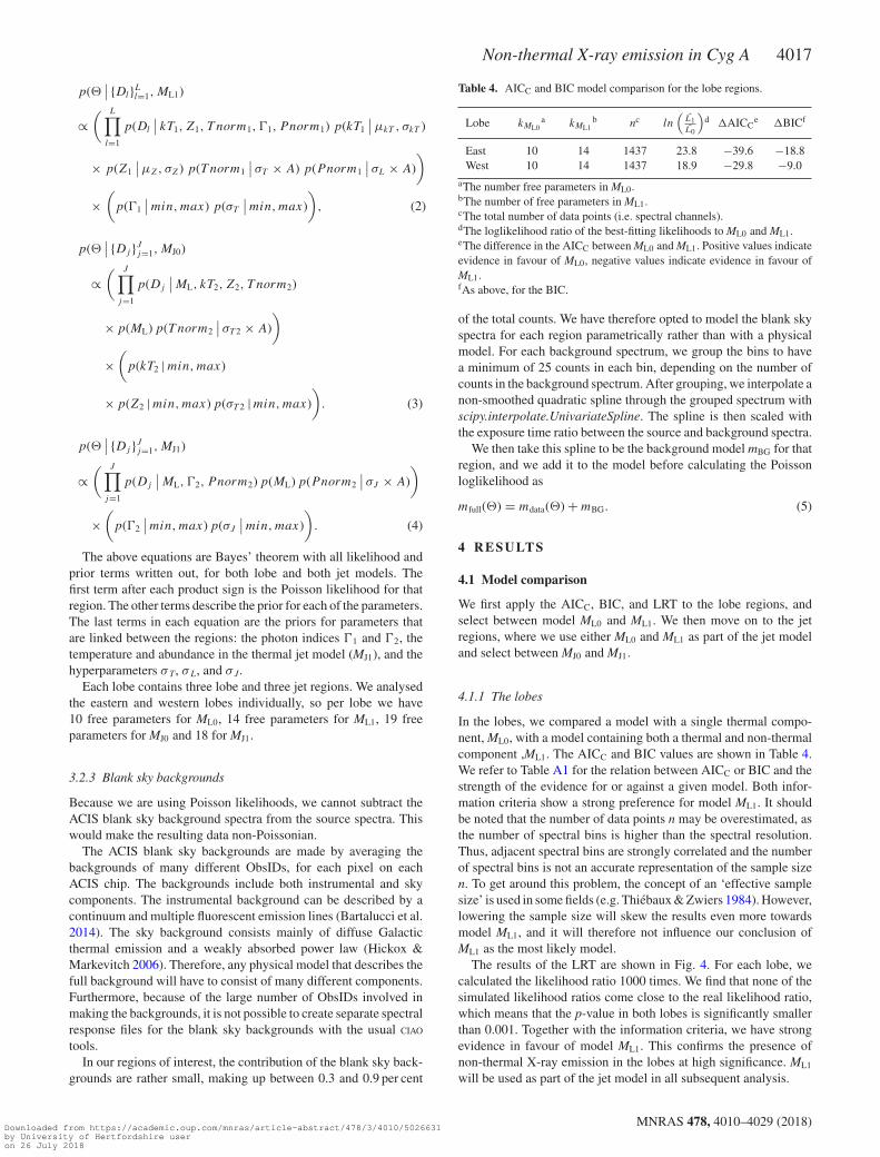
We can now write out the full posterior equations for lobe modelsML0 and ML1 and jet models MJ0 and MJ1, for lobe spectra Dl andjet spectra Dj:

p(∣∣ {Dl}L

l=1, ML0)

∝( L∏

l=1

p(Dl

∣∣ kT1, Z1, T norm1) p(kT1

∣∣μkT , σkT )

× p(Z1

∣∣μZ, σZ) p(T norm1

∣∣ σT × A)

)p(σT

∣∣min,max),

(1)



p(∣∣ {Dl}L

l=1,ML1)

∝( L∏

l=1

p(Dl

∣∣ kT1, Z1, T norm1, �1, Pnorm1) p(kT1

∣∣μkT , σkT )

× p(Z1

∣∣μZ, σZ) p(T norm1

∣∣ σT × A) p(Pnorm1

∣∣ σL × A)

)

×(

p(�1

∣∣min,max) p(σT

∣∣min,max)

), (2)

p(∣∣ {Dj }J

j=1, MJ0)

∝( J∏

j=1

p(Dj

∣∣ML, kT2, Z2, T norm2)

× p(ML) p(T norm2

∣∣ σT 2 × A)

)

×(

p(kT2 | min,max)

× p(Z2 | min, max) p(σT 2 |min, max)

). (3)

p(∣∣ {Dj }J

j=1, MJ1)

∝( J∏

j=1

p(Dj

∣∣ML, �2, Pnorm2) p(ML) p(Pnorm2

∣∣ σJ × A)

)

×(

p(�2

∣∣min, max) p(σJ

∣∣min, max)

). (4)

The above equations are Bayes’ theorem with all likelihood andprior terms written out, for both lobe and both jet models. Thefirst term after each product sign is the Poisson likelihood for thatregion. The other terms describe the prior for each of the parameters.The last terms in each equation are the priors for parameters thatare linked between the regions: the photon indices �1 and �2, thetemperature and abundance in the thermal jet model (MJ1), and thehyperparameters σ T, σ L, and σ J.

Each lobe contains three lobe and three jet regions. We analysedthe eastern and western lobes individually, so per lobe we have10 free parameters for ML0, 14 free parameters for ML1, 19 freeparameters for MJ0 and 18 for MJ1.

3.2.3 Blank sky backgrounds

Because we are using Poisson likelihoods, we cannot subtract theACIS blank sky background spectra from the source spectra. Thiswould make the resulting data non-Poissonian.

The ACIS blank sky backgrounds are made by averaging thebackgrounds of many different ObsIDs, for each pixel on eachACIS chip. The backgrounds include both instrumental and skycomponents. The instrumental background can be described by acontinuum and multiple fluorescent emission lines (Bartalucci et al.2014). The sky background consists mainly of diffuse Galacticthermal emission and a weakly absorbed power law (Hickox &Markevitch 2006). Therefore, any physical model that describes thefull background will have to consist of many different components.Furthermore, because of the large number of ObsIDs involved inmaking the backgrounds, it is not possible to create separate spectralresponse files for the blank sky backgrounds with the usual CIAO

tools.In our regions of interest, the contribution of the blank sky back-

grounds are rather small, making up between 0.3 and 0.9 per cent

Table 4. AICC and BIC model comparison for the lobe regions.

Lobe kML0a kML1

b nc ln(

L1L0

)d �AICC

e �BICf

East 10 14 1437 23.8 −39.6 −18.8West 10 14 1437 18.9 −29.8 −9.0

aThe number free parameters in ML0.bThe number of free parameters in ML1.cThe total number of data points (i.e. spectral channels).dThe loglikelihood ratio of the best-fitting likelihoods to ML0 and ML1.eThe difference in the AICC between ML0 and ML1. Positive values indicateevidence in favour of ML0, negative values indicate evidence in favour ofML1.fAs above, for the BIC.

of the total counts. We have therefore opted to model the blank skyspectra for each region parametrically rather than with a physicalmodel. For each background spectrum, we group the bins to havea minimum of 25 counts in each bin, depending on the number ofcounts in the background spectrum. After grouping, we interpolate anon-smoothed quadratic spline through the grouped spectrum withscipy.interpolate.UnivariateSpline. The spline is then scaled withthe exposure time ratio between the source and background spectra.

We then take this spline to be the background model mBG for thatregion, and we add it to the model before calculating the Poissonloglikelihood as

mfull() = mdata() + mBG. (5)

4 R ESULTS

4.1 Model comparison

We first apply the AICC, BIC, and LRT to the lobe regions, andselect between model ML0 and ML1. We then move on to the jetregions, where we use either ML0 and ML1 as part of the jet modeland select between MJ0 and MJ1.

4.1.1 The lobes

In the lobes, we compared a model with a single thermal compo-nent, ML0, with a model containing both a thermal and non-thermalcomponent ,ML1. The AICC and BIC values are shown in Table 4.We refer to Table A1 for the relation between AICC or BIC and thestrength of the evidence for or against a given model. Both infor-mation criteria show a strong preference for model ML1. It shouldbe noted that the number of data points n may be overestimated, asthe number of spectral bins is higher than the spectral resolution.Thus, adjacent spectral bins are strongly correlated and the numberof spectral bins is not an accurate representation of the sample sizen. To get around this problem, the concept of an ‘effective samplesize’ is used in some fields (e.g. Thiebaux & Zwiers 1984). However,lowering the sample size will skew the results even more towardsmodel ML1, and it will therefore not influence our conclusion ofML1 as the most likely model.

The results of the LRT are shown in Fig. 4. For each lobe, wecalculated the likelihood ratio 1000 times. We find that none of thesimulated likelihood ratios come close to the real likelihood ratio,which means that the p-value in both lobes is significantly smallerthan 0.001. Together with the information criteria, we have strongevidence in favour of model ML1. This confirms the presence ofnon-thermal X-ray emission in the lobes at high significance. ML1

will be used as part of the jet model in all subsequent analysis.



Figure 4. Top: Likelihood ratio distribution for ML0 and ML1 in the easternlobe. The likelihood ratio of the real data is shown as a red line. Bottom: Asabove, for the western lobe.

4.1.2 The X-ray jets

The model comparison tests in the lobe regions strongly prefermodel ML1 over ML0. Therefore, in the jet regions, we comparedtwo different models with three components, of which the firsttwo components are the thermal and non-thermal components ofML1. We added either a thermal component, MJ0, or a non-thermalcomponent, MJ1, to model the jet emission. The results of the modelcomparison between MJ0 and MJ1, with AICC and BIC, are listed inTable 5.

In the eastern jet, the likelihood ratio ln(

L1L0

)is negative, mean-

ing that the thermal model MJ0 has a higher likelihood than thenon-thermal model MJ1. However, because MJ0 has more param-eters, BIC prefers model MJ1 and AICC is close enough to zeroas to be inconclusive. In the western jet, both information crite-ria show clear preference for model MJ1. We note that, as in themodel selection of the lobes, the number of spectral channels nmight not be a correct representation of the amount of indepen-dent data points because the width of each channel is smaller thanthe spectral resolution of ACIS. Lowering n would bring the AICC

and BIC values closer to each other, skewing the AICC further to-wards MJ1 and the BIC towards MJ0. For example, setting n = 300,will yield �AIC = −1.2 and �BIC = −3.9 in the eastern jet and

Table 5. AICC and BIC model comparison for the jet regions.

Lobe kM0a kM1

b nc ln(

L1L0

)d �AICC

e �BICf

East 19 18 1437 −1.0 −0.2 −5.5West 19 18 1437 1.5 −5.0 −10.3

aThe number free parameters in MJ0.bThe number of free parameters in MJ1.cThe total number of data points (i.e. spectral channels).dThe loglikelihood ratio of the best-fitting likelihoods to MJ0 and MJ1.eThe difference in the AICC between MJ0 and MJ1. Positive values indicateevidence in favour of MJ0, negative values indicate evidence in favour ofMJ1.fAs above, for the BIC.

�AIC = −6.0 and �BIC = −8.7 in the western jet, indicatingmoderate to strong evidence for MJ1.

In the eastern jet, at the maximum posterior of model MJ0, wefind that a thermal X-ray jet would have T = 5.7 keV and Z = 0.21Z�. However, the spectral normalization of the jet component islower than what would be expected based on the surface brightness.For example, the spectral normalization of the jet in region J1 isabout 10 times lower than that of the ICM thermal component. Inthe western jet, a thermal jet would have T = 8.0 keV and Z = 0.10Z�, but the spectral normalization is multiple orders of magnitudebelow the ICM thermal component, or effectively zero.

Fig. 5 shows a comparison of models MJ0 and MJ1 in jet region J1,illustrating that the jet component has much lower normalization inMJ0. In both the eastern and the western side, the emission from thejet is mostly attributed to the ICM thermal emission. Optimizing theposterior does not produce reasonable parameters for a thermal jetmodel. Combined with the results from the AICC and BIC, whichall point in favour of model MJ1, we conclude that the favouredmodel includes a non-thermal emission component to describe thejet emission. In the analysis that follows, we will therefore usemodel ML1 in the lobe regions and MJ1 in the jet regions.

4.2 Thermal emission components

The results for the thermal properties of the background, lobe, andjet regions are listed in Table 6. As described in Section 3.2, the tem-peratures and abundances of the background regions were obtainedby fitting a PHABS X APECmodel to the spectra with SHERPA. Theobtained values were then used as priors for the lobe model, andthe distributions from the lobe models were in turn used as priorsfor the jet model. Table 6 shows that none of the temperatures andabundances within a set of background, lobe, and jet regions deviatesignificantly from each other.

Consistent with Snios et al. (2018) and Wise et al. (in preparation),we observe that the temperatures increase with distance from theAGN and significantly higher temperatures on the western sidethan on the east. Our results are also broadly consistent with thetemperatures found by Wilson et al. (2006) in the regions aroundthe lobe.

The inner background regions B3 and B4 are just on the edgeof the bright, rib-like structures extending outward from the AGN.Duffy et al. (2018) suggest that these rib-like structures are a resultof the destruction of the cool core during initial passage of the radiojet. Thermal plasma from the cool core would then be pushed intoa cylindrical rib-like shape by backflow antiparallel to the directionof the jet. The ribs have temperatures of around 2.5–4.5 keV (Chonet al. 2012; Duffy et al. 2018), making them significantly cooler



Figure 5. Comparison of models MJ0 (top) and MJ1 (bottom) in region J1.

Table 6. The thermal properties of the background, lobe, and jet regions.Background regions were fit with a PHABS x APEC model. The temper-atures and abundances are shown with 1σ errors. The temperatures andabundance posterior distributions of the lobe and jet regions are taken frommodels ML1 and MJ1.

Region kT (keV) Z(Z�) χ2/dof

B1 6.80 ± 0.30 0.41 ± 0.05 524.12 / 521L1 6.54+0.16

−0.16 0.47+0.05−0.05

J1 6.53+0.17−0.17 0.46+0.05

−0.05B2 6.30 ± 0.11 0.61 ± 0.04 684.04 / 625L2 6.35+0.10

−0.10 0.55+0.04−0.04

J2 6.36+0.11−0.11 0.55+0.04

−0.04B3 5.48 ± 0.12 0.68 ± 0.04 867.23 / 812L3 5.77+0.08

−0.08 0.72+0.03−0.03

J3 5.79+0.09−0.09 0.71+0.03

−0.03B4 5.91 ± 0.13 0.52 ± 0.04 805.63 / 774L4 5.97+0.20

−0.20 0.60+0.06−0.06

J4 6.06+0.20−0.21 0.58+0.05

−0.05B5 6.80 ± 0.20 0.49 ± 0.05 720.10 / 696L5 7.19+0.38

−0.32 0.53+0.07−0.06

J5 7.02+0.34−0.25 0.59+0.07

−0.06B6 7.72 ± 0.26 0.38 ± 0.05 707.86 / 711L6 8.03+0.46

−0.43 0.41+0.08−0.07

J6 8.00+0.46−0.43 0.42+0.08

−0.07

than the background regions. The background regions defined inthis work have a significantly higher temperature and thus can beassumed to be part of the cocoon shock, rather than the rib-likestructures. Table 6 does show a slightly worse fit quality regions B3and B4, which could indicate some mixing with enriched gas fromthe core. However, the reduced χ2 values in these regions, 1.07 forB3 1.03 for B4, show that these are still acceptable fits.

4.3 Non-thermal emission components

From the model comparison we conclude that there is non-thermalemission from both the lobes and the X-ray jets. This means that ineach set of lobe and jet regions, there are three non-thermal com-ponents and three associated normalizations: Pnorm1, L for the nor-malization of the lobe emission in the lobe region, Pnorm1, J for thenormalization of the lobe emission in the jet region, and Pnorm2, J

for the normalization of the jet emission. Correspondingly, thereare also three photon indices: �1, L for the lobe emission in the loberegions, �1, J for the lobe emission in the jet regions, and �2, J forthe jet emission. Because we used the posterior distributions fromthe lobe regions as a prior to constrain the lobe emission in the jetregion, we expect these posterior distributions to look similar. Wecomment further on this in Section 5.1.

We show the posterior distributions of the non-thermal emissioncomponents from the lobes and jets in Figs 6 and 7. We list thetotal flux and the photon index of each lobe and each jet in Table 7.We note that the lobe flux densities on the eastern and western sideare consistent with those found by Yaji et al. (2010) and Hardcastle& Croston (2010). For plots showing the correlation between thenormalization and photon index of each component in each region,we refer to Appendix B.

We compared the photon indices obtained from the posteriordistributions to the radio spectral index. Spinrad et al. (1985) findsan average low-frequency spectral index α of 0.74 for the lobes.This agrees well with our photon index of 1.72+0.03

−0.03 in the easternlobe, but not with the value of 1.97+0.23

−0.10 in the western lobe. Wediscuss possible causes for the differences between the lobes inSection 5.3.

4.4 Non-thermal pressure in the lobes and X-ray jets

4.4.1 The lobes

The parameters for the non-thermal emission that we find undermodel ML1 and MJ1 were used to model the pressure in the lobes.We compared the pressures found from the models with the rimpressures as calculated by Snios et al. (2018). These pressures aredetermined from X-ray spectra of compressed gas in regions be-tween the cocoon shock and the lobes. The average rim pressuresfor the eastern and western lobe are prim, east = (10.4 ± 0.4) × 10−10

erg cm−3 and prim, west = (8.4 ± 0.2) × 10−10 erg cm−3. By com-paring the rim pressures with the non-thermal pressures from ourmodels we are able to constrain lobe parameters such as the fractionof non-radiating particles and the lower limit to the electron energydistribution, denoted as κ and γ min, respectively.

The IC pressures were modelled with the IC code of Hardcas-tle, Birkinshaw & Worrall (1998), called synch. The code takesinto account both IC/CMB as well as SSC, which is an importantcomponent in the Cyg A lobes (Hardcastle & Croston 2010; Yajiet al. 2010). The code calculates the total energy density in a cer-tain volume, including the energy density from both particles and



Figure 6. Top: Posterior distributions for the power-law normalizations in the eastern lobe. Normalizations indicate the photon flux density at 1 keV. The toprow shows the non-thermal emission in each lobe region. The middle row shows the non-thermal lobe emission in each jet region, and the bottom row showsthe non-thermal jet emission each jet region. The solid lines indicate the median, the dashed lines the 14th and 86th percentiles. Bottom: As above, for thewestern lobe.

the magnetic field. We have modelled the electron distributions asbroken power laws with an age break.

We calculated the volume of each lobe by approximating them asa capped ellipsoid, inclined to the line of sight with an angle of 55deg (Vestergaard & Barthel 1993), based on the lobe region sizes.We obtain total volumes of 6.8 × 1068 cm3 for the eastern lobe, and7.4 × 1068 cm3 for the western lobe.

We normalized the synchrotron spectrum to the flux inside thelobe and jet regions on the 4.5 GHz VLA radio map (Carilli et al.1991). Because no radio brightness enhancement is observed at thelocation of the X-ray jet, we assume that all of the radio emissionin the lobe and jet regions can be attributed to the lobes. We findflux densities 211 Jy for the eastern lobe and 156 Jy for the westernlobe.

The break frequency νB varies over a range from 1 to 10 GHz inthe lobes of Cyg A (Carilli et al. 1991). We have modelled each lobewith a single average break frequency of 5GHz. We have assumedthat the photon index increases by 0.5 beyond the break frequency.Initial runs with synch show that the magnetic field in the lobesis around ∼40 μG. This translates to electron Lorentz factors ofγ B ∼ 7000 at the break frequency.

The choice for the lower cutoff to the electron energy distri-bution, γ min, can significantly affect the calculated pressure. Thehigher the photon index, the steeper the slope, and the more thelow-energy electrons contribute to the total pressure. The valueof γ min is unknown, we calculate the pressures for γ min = 1 andγ min = 10 . The upper cutoff to the electron distribution was set



Figure 7. Top: Posterior distributions for the power-law photon indices inthe eastern lobe. The top figure shows the photon index of the non-thermalemission in the lobe regions. The middle figure shows the photon index ofthe non-thermal lobe emission in the jet regions. The bottom figure showsthe photon index of the non-thermal jet emission in the jet regions. The solidlines indicate the median, the dashed lines the 14th and 86th percentiles.Bottom: As above, for the western lobe

Table 7. Flux density and power law of the non-thermal emission from thejets and lobes.

S1 keVa

(nJy) �

East Lobe 71+10−10 1.72+0.03

−0.03Jet 24+4

−4 1.64+0.04−0.04

West Lobe 50+12−13 1.97+0.23

−0.10Jet 13+4

−5 1.86+0.18−0.12

aFlux density at 1 keV.

at γ max = 105, giving a cutoff in the synchrotron spectrum at�1012 Hz.

The slope of the electron energy distribution, p, is directly relatedto the photon index by p = 2� − 1. We have used � from our modelsto determine p. We now have assumptions for γ min and γ max, thephoton indices and normalizations of the IC spectrum as determinedfrom the posterior distributions, and the normalization and νB of thesynchrotron spectrum determined from the VLA radio data. Withthese, the magnetic field strength and energy density in the lobe canbe modelled with synch.

We initially assumed an equipartition magnetic field and deter-mined what the predicted X-ray flux would be in this case, usingthe median value of the photon index posterior distribution. As-

Table 8. Comparison of the rim lobe pressures to the modelled IC lobepressures, for κ = 0.

prima γ min

b pICc B (μG)d

(10−10 erg cm−3) (10−10 erg cm−3)

East 10.4 ± 0.4 1 5.8+2.0−1.4 42+3

−310 2.2+0.4

−0.4 42+3−3

West 8.4 ± 0.2 1 140+1690−116 45+15

−510 18+40

−10 45+15−5

aThe rim pressures for the eastern and western lobe, taken from Snios et al.(2018).bThe lower cutoff to the electron energy distribution.cThe IC pressures, obtained from synch. See the text for details.dThe magnetic field strength, obtained from synch.

suming γ min= 1, we find equipartition fields of 95 and 210 μGin the eastern and western lobe, respectively. For γ min= 10, theequipartition fields are 73 and 130 μG. However, for both values ofγ min the equipartition field underpredicts the observed X-ray fluxby factors of a few, implying that the true magnetic field is belowthe equipartition value.

We then modelled the lobe pressure and magnetic field strengthby using the observed X-ray flux from the posterior distributions.For each lobe, we took 300 random samples of the non-thermalnormalization and photon index, and ran synch for each of theseparameter sets. The resulting distributions of the model pressure foreach lobe, and a comparison with the rim pressures, are shown inTable 8.

In the calculations above we have assuming that the fraction ofnon-radiating particles in the lobe, κ , is zero. Because the magneticfield strength is below equipartition, the total energy is dominatedby the particle energy. We can thus assume the IC pressures to scalelinearly with κ + 1.

As was previously reported by Hardcastle & Croston (2010), wefind that the non-thermal lobe flux in both lobes is dominated bySSC. In the eastern lobe, SSC makes up about 80 per cent of thetotal non-thermal flux. In the western lobe, the ratio spread is widerbecause of the wider distribution of �, but SSC makes up about50–90 per cent of the non-thermal flux.

4.4.2 The X-ray jets

We have modelled the X-ray jets as an IC emitting population ofelectrons, with synch. This corresponds to the IC relic jet modelproposed by Steenbrugge et al. (2008). The energy density andpressure in the X-ray jet can be calculated in the same manner asthe lobes and compared to the lobe and rim pressures on each side.

For the volume, we have used the defined jet regions and assumedthat they are tubular in shape. We also assume an inclination angleto the line of sight of 55 deg. This yields total volumes of 3.8 × 1067

and 4.2 × 1067 cm3 for the eastern and western jets, respectively.It is difficult to model the synchrotron spectrum from the X-ray

jets, because little to no emission is observed from these features.In the IC relic jet model, the adiabatic expansion of the jet shouldcause the Lorentz factors of the electron population to go down.The adiabatic expansion combined with synchrotron aging causedthe relic to have faded beyond detection at radio wavelengths.

We have looked for evidence of the relic jet in the LOFAR150 MHz data (McKean et al. 2016). In the eastern lobe, we observean enhancement in the brightness and spectral index map at roughlythe location of the relic jet. However, the enhancement seems to be



between two of the X-ray jet knots. In the western lobe, there is aslight brightness enhancement as well, although the correspondingspectral index enhancement is weaker than in the eastern lobe. Sim-ilarly, the enhancement is on the path of the relic jet, but not at thesame location as the X-ray jet knot. In both lobes, there seems to bea faint brightness enhancement that is roughly aligned with the pathof the relic jet. These brightness and spectral index enhancements,although weak and not well aligned, provide a hint that the X-rayjets are non-thermal in origin, consistent with our results from themodel comparison.

Regardless of whether the radio features seen in the LOFAR mapsare associated with the X-ray jet, it is difficult to determine whatthe radio spectrum of the IC relic jet would look like. We have usedthe LOFAR radio map to set an upper limit to the number density ofelectrons in the relic jet plasma. At most, the radio emission per unitvolume of the relic jet on the 150 MHz LOFAR map cannot be morethan that of the lobe. Using this assumption, we obtain maximumflux densities of 220 Jy at 150 MHz for the eastern jet, and 155 Jyat 150 MHz for the western jet. We note that this upper limit to theradio flux effectively corresponds to a lower limit on the modelledpressures. The lower the radio flux, the further below equipartitionthe relic jet will be, and the higher the modelled IC pressure.

While the relic jet only generates a relatively small number ofsynchrotron photons, it is embedded inside the lobe and subjectedto its synchrotron photon field. We therefore also considered athird IC component, which is the external Compton of the lobeand hotspot photon fields passing through the jet. We modelled thespectrum of the lobe by assuming that the radio emission mechanismis isotropic, and we assumed that the emission coefficient jν , is aconstant throughout the lobe. The average intensity at a specificwavelength is then

Jν = jν

∫dV

4π�2, (6)

where V indicates the volume, � the path along a ray from the sourceto the region of interest, and Jν the average intensity. We assumeaxial symmetry for the lobe, and use cylindrical polar coordinatesr, φ, z. Then, integrating over the angle φ yields

Jν = jν

∫r dr dz

2√

{z2 + (r − x0)2}{z2 + (r + x0)2} , (7)

where x0 is the distance from the axis of the point of interest in theplane z = 0. We evaluate the intensity at the centre of the jet (x0 = 0).We also assume the jet is a cylindrical tube inside the lobe, and sowe integrate over the cylinder radius r between rj(z) and rl(z). Thisreduces the integral to a one-dimensional integral over z:

Jν = jν

4

∫ln(z2 + r2

l

z2 + r2j

)dz. (8)

The radius of the lobe and the jet, rj and rl, are both functions ofz. We have approximated both functions for each lobe by manuallymeasuring the radius at several points along the z-axis and linearlyinterpolating between these points.

We used equation (8) along with the radio flux from the VLA data,to calculate the average intensity at 4.5 GHz. We then modelled thespectrum of the lobe as a broken power law, using a break frequencyof 5GHz. The spectral index of the lobe model is drawn directlyfrom the posterior distributions and therefore varies from sample tosample.

Additionally, we estimated the influence from the hotspots bymodelling them as point sources. We again took the radio flux ofthe hotspots from the VLA data, finding flux densities of 117 Jy for

Table 9. The IC relic jet pressures, for κ = 0.

γ mina pIC

b B (μG)c

(10−10 erg cm−3)

East 1 7.9+5.8−3.3 27+5

−410 4.0+2.6

−1.3 27+5−4

West 1 99+540−76 17+7

−310 22+40

−12 17+7−3

aThe lower cutoff to the electron energy distribution.bThe IC pressures, obtained from synch. See the text for details.cThe magnetic field strength, obtained from synch.

the eastern hotspots and 152 Jy for the western hotspots. We thencalculated the average flux between the minimum and maximumhotspot–jet distance. We modelled the hotspot spectrum as a brokenpower law, with a break frequency at 10 GHz and a photon indexof 1.5.

Because the spectrum of the relic jet is unknown, an assumptionfor the break frequency has to be made. If the break frequency in theradio spectrum is too low, the IC spectrum would have a turnoverbelow the 0.5–7.0 keV range, and the photon index that we see inthe X-ray data would be the photon index beyond the turnover. Weconsider this unlikely, especially in the eastern X-ray jet, as theslope before the turnover would then be as flat as ∼1.1. This placesconstraints on how low the break frequency can be. By modelling thejets with synch, we find that the break frequency should not be lowerthan ∼4 GHz. Below that value, Compton scattering of synchrotronphotons originating from the lobes, the dominant component inthe X-ray jet flux, starts to turn over enough that it noticeablyaffects the slope of the total IC spectrum. We therefore place thebreak frequency at this value. The break frequency of 4 GHz anda magnetic field strength of 30 μGcorrespond to an electron breakLorentz factor γ B∼ 7000. The same cutoffs and lower and upperlimits were applied as for the lobes: the minimum frequency for thesynchrotron spectrum is 1 MHz. The jet pressures were calculatedfor γ min = 1 and γ min = 10. The maximum electron Lorentz factorwas set at γ max = 105 , which gives a cutoff in the synchrotronspectrum at ∼1013 Hz.

We calculated the distribution of model pressures the same wayas for the lobes: we took 300 random samples from the posteriordistributions of the jet normalization and photon index. We as-sumed κ = 0 and we calculate pressures for both γ min = 1 andγ min = 10. The results are listed in Table 9. We find that externalCompton scattering dominates the total flux. In the eastern jet, wefind that the external Compton from the lobe photons contributesapproximately 65 per cent to the total flux, SSC of the jet photonsapproximately 15 per cent, and IC/CMB scattering 20 per cent. Inthe western jet, the wider distribution of � causes a greater spreadin these fractions. External Compton of the lobe photons contributes40−60 per cent, SSC of the jet photons 5−30 per cent and IC/CMBscattering 5−40 per cent. This shows that the relic jet is not purelyan IC/CMB X-ray source, but that SSC needs to be taken into ac-count in an IC relic jet model.

5 D ISCUSSION

5.1 Disentangling the lobe and jet emission components

The fact that the model in the jet regions contains two separatepower laws with similar photon indices, means that degeneraciesare a concern. It is possible that the MCMC routine in the jet regions



does not manage to fully disentangle the lobe emission from the jetemission. We have attempted to minimize this problem by makingthe amount of lobe emission in the lobe regions a prior for theamount of lobe emission in the jet regions. By assuming that thesurface brightness of the non-thermal lobe emission is constant,the MCMC routine has less difficulty separating the non-thermalemission in the jets into two different components.

From the middle and bottom rows of both panels of Fig. 6, itappears that the two power laws can be distinguished from one an-other in every region. If they were not, we would expect to see mostof the non-thermal emission attributed to just one of the power lawsand the other posterior distribution approaching zero. Instead, theresults show distinct unimodal peaks for the lobe component andthe jet component in each jet region. Because we used the posteriordistributions of Pnorm1, L and �1, L from the lobe model as priors forthe parameters Pnorm1, J and �1, J in the jet model, we expect theposterior distributions of the corresponding jet and lobe parametersto be very similar. We compared the prior distributions to test this,and find that the median and the spread of each distribution agreesto a few per cent precision. This indicates that the MCMC routinefor the jet regions did not stray far from the prior distributions givenby the MCMC sampling of the lobe regions. Our assumption of con-stant surface brightness between a lobe region and its correspondingjet region seems therefore to be reasonable.

We investigated whether the ratio of jet to lobe flux on each side,obtained from the posterior distributions, agrees with the jet to lobecount ratio from the event data. The count ratio is determined fromthe event files as follows: we determine the number of counts inthe jet region. We then subtract the number of counts in the loberegion, scaled to the area of the jet region. We then assume that 50–70 per cent of the counts in the lobe region are thermal, and subtractthis number from both the lobe and the jet. We are then left withestimates for the number of non-thermal counts in the lobe and thejet. In the eastern lobe, we find a flux ratio of 1.5+0.6

−0.4, and a countratio of 2.0–2.7. On the western side, we find a flux ratio of 1.1+0.9

−0.6

and a count ratio of 1.7–2.1.The count ratio is slightly higher than the flux ratio on both sides,

which raises the possibility that our model underestimates the jetflux. However, the higher count ratio translates to only a modestdifference in the jet flux. In the eastern jet, a count ratio of 2.0–2.7corresponds to a jet flux of 26–28 nJy, while in the western jet acount ratio of 1.7–2.1 corresponds to a jet flux of 15–17 nJy. Bothestimates are within the errors of the jet flux distribution from themodel. The estimate provided by the count ratio seems to agree wellwith the flux ratio obtained from the model.

5.2 A two-temperature thermal model for the ICM

As shown in Section 4.2, there is a significant difference betweenthe ICM on the eastern and the western side of Cyg A. The temper-ature increase on the western side is in the direction of the mergerwith nearby subcluster Cyg NW, and roughly corresponding to thedirection of the outburst. The fact that the temperature increase isonly on one side would suggest that a shock created by the mergeris the underlying cause of the temperature increase. Moreover, itis possible that the merger shock has enhanced features that werealready there, perhaps imprints of previous cycles of AGN activity,or features created by sloshing motions. For a more extended dis-cussion of the complex merger region, we refer to Wise et al. (inpreparation).

Regardless of the cause of the temperature difference betweeneast and west, there is reasonable cause to suspect that the ICM

surrounding the western cocoon shock may actually be better de-scribed by a two-temperature thermal plasma. For example, onecould imagine a geometry where the ICM shocked by the merger isa layer of hot ∼10 keV material that is partly projected in front ofthe lobe, while the underlying ICM has a temperature of ∼6 keV,the same as on the eastern side.

Mazzotta et al. (2004) have investigated the effect of fittinga single-temperature thermal model to a two-temperature plasmawith Chandra. For high gas temperatures (>5 keV, and low abun-dances (<1.0 Z�), they find that a single-temperature thermalmodel fit is often statistically indistinguishable from a fit with atwo-temperature thermal model. This is because when the gas tem-perature is high, the gas will be more highly ionized, making itmore difficult to distinguish spectra with differing temperatures.In the case of Cyg A’s western lobe, assuming two-temperaturecomponents of ∼6 and ∼10 keV, and an abundance of ∼0.5 Z�,the results from Mazzotta et al. (2004) indicate that the emissionfrom this plasma would be very well fit by a single-temperaturethermal model. Although the structure of the hot plasma aroundthe western lobe might be complex, we therefore expect that usinga single-temperature thermal model provides an adequate enoughdescription of the spectral data.

5.3 Difference between the eastern and western lobes

The posterior distributions show clear differences between the east-ern and western side, with the western side being both fainter andhaving a steeper X-ray spectrum. The steeper X-ray spectrum mapsonto a steeper electron spectrum with a larger fraction of electronenergies with low γ . This translates into higher energy densitiesand pressures on the western side.

The photon index on the eastern side agrees well with the valueof Spinrad et al. (1985), as well as with the spectral index obtainedfrom the LOFAR data by McKean et al. (2016). All of these showaverage spectral indices α ∼ 0.7.

If the photon index in the western lobe accurately reflects theaverage photon index, we suggest that either aging or adiabaticlosses may have caused a turnover in the IC spectrum somewherebelow 7.0 keV. This would explain why the photon index is higherand less constrained. It would also mean the pressures calculatedby synch are overestimated on the western side, because the low γ

range of the electron energy spectrum would have a lower photonindex than we have modelled.

We looked at the available VLA and LOFAR data to see if thereare differences between the lobes in the radio. In both radio maps,we find that the western lobe is roughly 30 per cent fainter than theeastern lobe. However, there appear to be no appreciable differencesbetween the lobes in terms of spectral index and break frequency(Perley et al. 1984; McKean et al. 2016).

Snios et al. (2018) estimate that the total volume of the westernlobe is about 40 per cent larger than the eastern lobe. Their estimateincludes the volume of the shocked cocoon not just of the lobes.We note that in our own estimate of the lobe volume, the westernlobe is only about 10 per cent larger than the eastern lobe. However,the lobe regions that we have defined do not exactly follow theradio lobe, and also have the hotspot regions cut out. Therefore, thevolume calculated from the lobe regions is not necessarily accuratefor the lobe as a whole.

If the western lobe is indeed bigger than the eastern lobe by afew tens of percent, then this could indicate additional adiabatic ex-pansion on the western side, which would reduce both the magneticfield strength and the particle energies. Under simple assumptions



for adiabatic expansion, B ∝ V−2/3 and γ ∝ V−1/3, which means wewould expect the magnetic field strength in the western lobe to be80 per cent of that in the eastern lobe. The magnetic field strengths inTable 8 do not differ significantly between east and west, althoughthe errors on the western side are large.

For a synchrotron spectrum, the Lorentz factor of an emittingelectron and the emitted frequency are related as

ν � γ 2qB

2πme

, (9)

while in the corresponding SSC spectrum, the Lorentz factor isrelated to the energy as

E = γ 4�qB

me

. (10)

Equation (10) and the scaling relations for B and γ imply that thecharacteristic energy scales with the volume as E ∝ V−2. If thewestern lobe is 40 per cent bigger, the turnover in the IC spectrumof the western lobe could therefore be at 50 per cent of the energyof that of the eastern lobe.

A break frequency νB at 5 GHz and a magnetic field strength ofaround 40 μG, yield break Lorentz factor γ B ∼ 7000, and a breakenergy EB∼ 1 keV. This means that a turnover of the SSC part of thespectrum would be a plausible explanation for the steeper spectrumin the western lobe, especially because SSC makes up a significantamount of the total non-thermal flux in the lobes. To look for ev-idence of a spectral turnover, we re-evaluated the lobe spectra intwo separate energy bands of 0.5–2.0 and 2.0–7.0 keV. We repeatedthe MCMC analysis of model ML1 in both lobes, allowing eachenergy band to have a different photon index. In the eastern lobe,we find �0.5−2.0 = 1.56+0.07

−0.07 and �2.0−7.0 = 1.72+0.04−0.04. In the western

lobe, we find �0.5−2.0 = 1.80+0.19−0.11 and �2.0−7.0 = 1.94+0.25

−0.10. Whilethe errors in the western lobe are too large to distinguish betweenthese photon indices with any statistical certainty, the numbers areconsistent with the possibility that we are indeed seeing a turnoverin the non-thermal X-ray spectrum of the western lobe. Somewhatmore surprising is that a similar effect is also observed in the easternlobe, given that the photon index of 1.72+0.03

−0.03 agrees well with theradio data, and we do not expect the average photon index to besignificantly lower than this. However, we note that our models arelimited by the fact that each lobe and jet are modelled with only asingle photon index. Therefore, the variation seen between the lowand high energy bands on both sides should be taken as a sign thatthe true electron energy distributions are more complicated thanassumed here.

The correlation plots in Fig. B1 provide further insight as to whythe photon index in the west is higher. In the eastern lobe, the modelshows a non-thermal surface brightness in region L1 that is clearlylarger than in regions L2 and L3. This is consistent with the radiomaps, which show more continuum emission closer towards thehotspots. By contrast, in the western lobe, L6 is not significantlybrighter than regions L4 and L5. If the X-ray photon index followsthe radio spectral index, we would expect it to be significantly highercloser towards the AGN. Therefore, the reason that the photon indexin the western lobe is higher could be explained by the fact that L4and L5 contribute more to the total flux in the west than L2 and L3do in the east. Because these inner regions have a higher photonindex, the average photon index for the entire lobe will also behigher.

This raises the question, what has caused the underlying discrep-ancy? As we have discussed at the beginning of this section, it ispossible that the environment in the lobes and jets itself is different,

and that the turnover in the western side is at lower energies than onthe eastern side. Additionally, Snios et al. (2018) have shown thatthe shock on the eastern side is stronger, and so the shock could havemanaged to create more energetic particles in region L1, pushingthe average photon index in the eastern lobe to a lower value. A thirdpossibility is that the geometrical assumptions that we have madehave influenced the results. In particular, the assumptions that linkthe normalizations of emission components between correspondingbackground, lobe, and jet regions might be inaccurate, perhaps be-cause the western lobe is less symmetric than the eastern lobe. Thiswould cause too much or too little emission to be attributed to oneof the emission components.

5.4 Contribution of infrared photons to the IC flux

In the analysis of the emission from the lobes and X-ray jets wehave considered synchrotron and CMB photons as seed photonsfor the IC process. However, infrared photons emitted from theAGN and the dust around the AGN can additionally provide asignificant contribution to the total IC flux (Brunetti et al. 1997). Inthis section, we estimate approximately how much these photonswould contribute to the IC flux.

Weedman et al. (2012) calculate the strength of several IRspectral features in Cyg A, but do not provide a value for thetotal infrared luminosity LIR. However, we have made use ofthe scaling relationship between νLν(7.8μm) and LIR, which islog [LIR/νLν(7.8μm)] = 0.80 ± 0.25 in AGN with silicate absorp-tion (Sargsyan et al. 2011). Using the value of fν(7.8μm) = 54 mJyfrom Weedman et al. (2012) and using the upper limit of the scalingrelationship, we find LIR ∼ 1.8 × 1045 erg s−1. This is consistentwith the scaling relationship between bolometric luminosity and in-frared luminosity found in that same paper, using Lbol ∼ 3.8 × 1045

erg s−1 from Privon et al. (2012).We calculated the number density of infrared photons in the lobe

as NIR = LIR/(4πcd2EIR), where we have used d = 40 kpc as anaverage distance in the middle of the lobe, and EIR = 3.3 × 10−14 erg(λIR = 60 μm) as the characteristic energy of an infrared photon,corresponding to the peak of the SED (Privon et al. 2012). Thisyields NIR = 10 cm−3. Meanwhile, the energy density of the CMBis uCMB = 4.1 × 10−13(1 + z)4 erg cm−3 (Harris & Grindlay 1979),yielding a photon number density NCMB = 360 cm−3.

While the number density of CMB photons is larger, we alsohave to take into account that infrared photons have higher en-ergy and therefore have access to a larger number of electronsto be IC scattered to keV energies. A 60 μm photon requiresγ ∼ 200 to be upscattered to 1 keV, while a CMB photon re-quires γ ∼ 1000 to be upscattered to 1 keV. Using the slope ofthe electron spectrum p = 2.4 in the eastern lobe, we find a rel-ative electron number density of Nγ1000/Nγ200 = 0.11. For the fluxratio at 1 keV of IC/CMB flux to infrared IC flux, we then estimatefCMB/fIR ∼ NCMBNγ1000/NIRNγ200 = 4.

The modelling in Section 4.4 has shown that synchrotron radi-ation is the dominant component in both lobes, and that the CMBmakes up between 10 and 50 per cent of the flux. If the IC/CMBflux is four times higher than the infrared IC flux, as our estimateindicates, the infrared IC flux would contribute 2.5–12.5 per cent tothe total IC flux.

We expect that including the infrared spectrum as an additionalphoton field in our model would reduce the pressures, as fewerelectrons would be needed to produce the same X-ray flux. However,since the maximum contributions of the infrared photons are less



than the errors in the pressures, including them in the model wouldnot have significantly altered our results.

5.5 The X-ray jets as IC relic jets

MCMC sampling of the Bayesian models for the jets and lobes ofCyg A has yielded good constraints on their photon indices andflux densities. However, turning these into pressures introduces ad-ditional errors. The pressure is strongly dependent on the photonindex in particular, which leads to very large uncertainties, partic-ularly in the western lobe. Additionally, it is not known what theradio spectrum of the relic jet would be. This has forced us to makeassumptions about the shape of the spectrum.

The magnetic field strengths found in Table 8 are a factor of 2–6below equipartition. This seems to be a typical value for FRII radiogalaxies (Croston et al. 2005; Ineson et al. 2017). We compare therim pressures with the IC pressure listed in Table 8 to constrain theparticle content κ in the lobes. In the eastern lobe, the assumptionof κ = 0 yields a pressure that is inconsistent with the rim pressure.Depending on the choice of γ min, we require 1 < κ < 5 in the east-ern lobe to match the rim pressures. Croston & Hardcastle (2014)developed a model for FRI radio galaxies where jet entrainmentof protons/ions could provide the necessary additional pressure. Asimilar process could also be at work here.

On the eastern side, if κ and γ min in the jet have the same valueas in the lobe, the lobe and jet pressure are the same within theerrors. However, it is unclear what determines the particle contentof the jet and how it is related to the particle content in the lobe.It is possible that κ in the jet is lower or higher than in the lobe.On the western side, the calculated jet and lobe pressures are thesame within the errors as well, assuming the same κ and γ min. Atκ = 0 and γ min = 1, both of these pressures are much higher thanthe western rim pressure. This would imply that κ = 0 and that γ min

is larger than in the eastern side. However, it is difficult to imaginea scenario where κ is significantly different between the easternand western side. Given the discrepancy in photon indices, and thepossibility of a turnover in the western side due to adiabatic losses oraging effects, we consider it more likely that we have overestimatedthe western lobe and jet pressures, as discussed in Section 5.3.

Another possibility is that γ min is higher than assumed in ouranalysis. A consequence of the steeper spectrum on the westernside is that the pressure falls off more quickly with increasing γ min.Therefore, if γ min is higher on the western side than on the easternside, it is possible to make the western lobe pressure consistent withthe eastern lobe pressure.

We note that our relic jet model is significantly different fromthe pure IC/CMB jet with very low magnetic field, proposed bySteenbrugge et al. (2008). As already noted in Section 1, a problemof the IC/CMB jet model is that it requires a significantly higherelectron density, which would result in much higher electron pres-sures in the jet. In our model, the magnetic field in the X-ray jet islower than in the lobes by a factor of ∼ 35−65 per cent. This allowsfor a higher electron density in the jet while still producing lesssynchrotron radiation than the lobe. At the same time, the magneticfield is still high enough that the produced synchrotron photons areenergetic enough to be IC scattered to the keV energy range. In thisway, SSC can be the dominant component of IC flux in the jet, andthe electron density can be much lower than in a pure IC/CMB jet.However, it means that our model can only exist in a narrow regionof parameter space. While the model shows how the X-ray jet couldin principle exist as an IC relic, it raises the question of why theelectron spectrum in the jet would have exactly this shape.

An additional complication of the relic jet model is the existenceof jet knots. In modelling the jet pressures, we have assumed thatthe X-ray emission per unit volume is uniform throughout the jet.However, the deep Chandra exposure of the system reveals thatthere are several bright jet knots, most notably on the eastern side.We estimated the contrast of these brightness variations. We tookthe average counts per pixel in regions J1–J3, and subtracted theaverage counts per pixel from L1–L3. We find 40 counts per pixelon average in L1–L3, with a minimum of 5 and a maximum of 80counts in a pixel. We repeated the procedure on the western side andfound a pixel average of 15 counts, with minimum 0 and maximum38 counts. This shows that there are significant brightness variationsin both jets. This implies large variations in pressure along the jet.

To test the pressure variations in our model, we took one of thebrightest parts of the eastern jet, in the middle of region J2. Wedefined a square region with the same width and orientation as theJ2 jet region, and with a length of 4.5 arcsec centred on the brightestpart. We then determined the background-subtracted average countsper pixel in this region to be 67 counts, or 1.67 times the averagecounts per pixel over the entire jet. We then ran synch for this region,using a flux density of 1.67 times higher than the flux density foundin the eastern jet. The radio flux was scaled to the volume of theemitting region, but was not increased by a factor of 1.67, as theradio flux from the X-ray jet region is an upper limit. Modelling thejet knot in this way, we find pressures of ∼13 × 10−10 erg cm−3

for γ min = 1 or ∼6 × 10−10 erg cm−3 for γ min = 10. This narrowsthe range of parameters pressure balance with the surrounding lobesomewhat, especially given the fact that γ min is likely to be low inthe relic jet.

Unfortunately, the assumptions that we have made in trying tomodel the jet-like features are just too uncertain to be able to drawany definite conclusions about how whether the IC relic jet modelis sustainable in Cyg A. While we find slightly higher pressures inthe eastern jet compared to the lobe, both κ and γ min are unknownquantities that can greatly influence the pressure in the relic jet.

Although we cannot rule out an IC relic jet model based on theX-ray and radio spectra, it is unclear how these knots of brightemission in the X-ray jets could be maintained in the IC relic jetmodel, where the radio jets have expanded by a factor of a few fromtheir original, rather narrow size. If the knots originate from theradio jet, and if the X-ray jet has reached pressure equilibrium withthe surrounding lobe, the knots should have been smoothed out inthe process.

6 C O N C L U S I O N

Deep Chandra observations of the X-ray jets and lobes of Cyg Ahave allowed us to analyse the emission from these features in detail.In the lobes, we have used two different tests to compare thermaland non-thermal models. In both lobes, we find that spectral fitsstrongly prefer a model with a non-thermal emission component forthe lobe emission. In the X-ray jets, we used the thermal and non-thermal components of the ICM and lobe emission, and comparedbetween a model with an additional thermal or additional non-thermal component for the jet emission. We find that the modelwith a non-thermal component for the jet is moderately to stronglypreferred.

MCMC sampling of the non-thermal lobe and jet models hasgiven us constraints on the flux and photon indices of the jets andlobes. For the eastern lobe and jet, we find 1 keV flux densities of71+10

−10 and 24+4−4 nJy, and photon indices of 1.72+0.03

−0.03 and 1.64+0.04−0.04,

respectively. For the western lobe and jet, we find flux densities of



50+12−13 and 13+5

−5 nJy, and photon indices of 1.97+0.23−0.10 and 1.86+0.18

−0.12,respectively.

For each lobe, we used broken power laws with an age breakto model the electron energy distributions. A comparison with therim pressures from Snios et al. (2018) shows that a significantpopulation of non-radiating particles is required to account for thetotal pressure of the eastern lobe. We also find a magnetic fieldof around 40 μG, a factor 2 lower than the equipartition value of73–95μG . This ratio of B/Beq agrees well with a sample of otherFRII radio galaxies (Ineson et al. 2017).

However, in the western lobe no population of non-radiatingparticles is required and the low energy cutoff of the electron dis-tribution needs to be raised to obtain a pressure consistent with therim pressure. This discrepancy is a consequence of the difference inphoton index between the two lobes, and suggests that the true elec-tron distributions may be more complex than a single broken powerlaw. A possible cause for the discrepancy is that the SSC componentof the spectrum in the western lobe could have a turnover at lowerenergies than in the eastern lobe, perhaps because of the differencein size. A spectral turnover below a few keV would yield a higherphoton index in the 0.5–7.0 keV energy range. The data are slightlysuggestive of a turnover in this range, with a lower photon indexbetween 0.5 and 2.0keV than at 2.0 and 7.0keV, although the con-straints are not strong. A further complicating factor is the fact thatthe photon index likely is not constant throughout the lobe. Thecorrelation plots in AppendixB show that the inner regions on thewestern side (L4 and L5) contribute more to the total flux than theinner regions on the eastern side (L2 and L3). Because these regionspresumably have a higher photon index, the average photon indexfor the western lobe will be higher as well.

Regardless of the cause, if the photon index in the western lobe isoverestimated, then the pressures on that side are overestimated aswell. We consider the photon index in the eastern lobe more likelyto be accurate because it agrees well with values in the literature ofthe average radio spectral index in the lobes.

We modelled the X-ray jets according to the IC relic jet modelfrom Steenbrugge et al. (2008). Similar to the lobes, we used theX-ray and radio data to constrain the spectra and model the electrondistributions. On the 150 MHz LOFAR data, a weak brightnessenhancement is seen at roughly the location of the relic jet, althoughimperfectly aligned. This could indicate the presence of the IC relicjet in radio wavelengths, but the emission is too weak to be able toconstrain the radio synchrotron spectrum. Therefore, assumptionshave to be made about the normalization of the radio frequency andthe break frequency. Moreover, γ min and κ are poorly constrained,making the modelling uncertain.

We find a higher median pressure in the eastern jet compared tothe lobe, but still within the errors. This suggests that an IC relic jetcould be relatively close to pressure balance with the surroundinglobe. However, the IC relic jet model as we have modelled it can onlyexist in the narrow region of parameter space. The magnetic fieldneeds to be lower than in the lobe, so that the jet is not brighter thanthe lobe in the radio. At the same time, if the IC flux is dominatedby SSC, the magnetic field needs to be high enough to producesynchrotron photons that can be scattered to the keV energy range.

An additional problem is that the model does not take into accountthe jet knots of increased brightness. If these knots originate fromthe radio jet, we would expect them to have been smoothed outin the process of adiabatic expansion if the current jet is closeto achieving pressure balance with the lobe. Better constraints onthe synchrotron spectrum, and more detailed modelling to allow for

variations in flux and photon index along the jet axis, will be neededto shed more light on the nature of the jet-like X-ray features in CygA.

AC K N OW L E D G E M E N T S

We would like to thank the anonymous referee for their useful com-ments on the draft version of this paper. Support for this work wasprovided by the National Aeronautics and Space Administrationthrough Chandra Award Number GO5-16117A issued by the Chan-dra X-ray Observatory Center, which is operated by the SmithsonianAstrophysical Observatory for and on behalf of the National Aero-nautics Space Administration under contract NAS8-03060. PEJNwas supported in part by NASA contract NAS8-03060. MJH ac-knowledges support from the UK Science and Technology FacilitiesCouncil [ST/M001008/1].

REFERENCES

Akaike H., 1974, IEEE Transactions on Automatical Control , 19, 716Anders E., Grevesse N., 1989, Geochim. Cosmochim. Acta, 53, 197Bartalucci I., Mazzotta P., Bourdin H., Vikhlinin A., 2014, A&A, 566, A25Brunetti G., Setti G., Comastri A., 1997, A&A, 325, 898Burnham K. P., Anderson D. R., 2002, Model Selection and Multimodel In-

ference: A Practical Information-Theoretic Approach, Springer-VerlagBırzan L., Rafferty D., McNamara B., 2004, ApJ, 607, 800Carilli C. L., Perley R. A., Dreher J. H., 1988, ApJ, 334, L73Carilli C. L., Perley R. A., Dreher J. W., Leahy J. P., 1991, ApJ, 383, 554Carilli C. L., Perley R. A., Harris D. E., 1994, MNRAS, 270, 173Celotti A., Ghisellini G., Chiaberge M., 2001, MNRAS, 321, L1Chon G., Bohringer H., Krause M., Trumper J., 2012, A&A, 545, L3Croston J., Hardcastle M., Harris D., Belsole E., Birkinshaw M., Worrall

D., 2005, ApJ, 626, 733Croston J. H., Hardcastle M. J., 2014, MNRAS, 438, 3310Croston J. H., Hardcastle M. J., Birkinshaw M., Worrall D. M., Laing R. A.,

2008, MNRAS, 386, 1709Dickey J. M., Lockman F. J., 1990, ARA&A, 28, 215Dreher J., Carilli C., Perley R., 1987, ApJ, 316, 611Duffy R. T. et al., 2018, MNRAS, 476, 4848Fanaroff B., Riley J., 1974, MNRAS, 167, 31Foreman-Mackey D., Hogg D. W., Lang D., Goodman J., 2013, PASP, 125,

306Freeman P., Doe S., Siemiginowska A., 2001, in Starck J.-L., Murtagh

F. D., eds, Proc. SPIE Vol. 4477, Astronomical Data Analysis. SPIE,Bellingham, p. 76

Fruscione A. et al., 2006, in Silva, D. R., Doxsey, R. E., eds., Proc. SPIE,Vol. 6270. SPIE, Bellingham, p. 62701V

Gelman A., 2006, Bayesian Anal., 1, 1Goodman J., Weare J., 2010, Commun. Appl. Math. Comput. Sci, 5, 65Hardcastle M., 2006, MNRAS, 1465Hardcastle M., Croston J., 2010, MNRAS, 404, 2018Hardcastle M. et al., 2016, MNRAS, 455, 3526Hardcastle M. J., Birkinshaw M., Worrall D. M., 1998, MNRAS, 294, 615Hardcastle M. J., Kraft R. P., Worrall D. M., Croston J. H., Evans D. A.,

Birkinshaw M., Murray S. S., 2007, ApJ, 662, 166Hardcastle M. J., Worrall D. M., Birkinshaw M., Laing R. A., Bridle A. H.,

2002, MNRAS, 334, 182Harris D. E., Grindlay J. E., 1979, MNRAS, 188, 25Hickox R. C., Markevitch M., 2006, ApJ, 645, 95Hinshaw G. et al., 2013, ApJS, 208, 19Ineson J., Croston J. H., Hardcastle M. J., Mingo B., 2017, MNRAS, 467,

1586Jeffreys H., 1961, Theory of Probability, Oxford University Press, OxfordJester S., Harris D. E., Marshall H. L., Meisenheimer K., 2006, ApJ, 648,

900


http://dx.doi.org/10.1016/0016-7037(89)90286-X

http://dx.doi.org/10.1086/383519

http://dx.doi.org/10.1086/185315

http://dx.doi.org/10.1086/170813

http://dx.doi.org/10.1093/mnras/270.1.173

http://dx.doi.org/10.1046/j.1365-8711.2001.04160.x

http://dx.doi.org/10.1086/430170

http://dx.doi.org/10.1093/mnras/stt2436

http://dx.doi.org/10.1111/j.1365-2966.2008.13162.x

http://dx.doi.org/10.1146/annurev.aa.28.090190.001243

http://dx.doi.org/10.1086/165229

http://dx.doi.org/10.1093/mnras/167.1.31P

http://dx.doi.org/10.1086/670067

http://dx.doi.org/10.1214/06-BA117A

http://dx.doi.org/10.2140/camcos.2010.5.65

http://dx.doi.org/10.1093/mnras/stv2553

http://dx.doi.org/10.1111/j.1365-8711.1998.01159.x

http://dx.doi.org/10.1086/517997

http://dx.doi.org/10.1046/j.1365-8711.2002.05513.x

http://dx.doi.org/10.1093/mnras/188.1.25

http://dx.doi.org/10.1086/504070

http://dx.doi.org/10.1088/0067-0049/208/2/19

http://dx.doi.org/10.1086/505962


Kalberla P. M. W., Burton W. B., Hartmann D., Arnal E. M., Bajaja E.,Morras R., Poppel W. G. L., 2005, A&A, 440, 775

Kass R. E., Raftery A. E., 1995, JASA , 90, 773Konar C., Hardcastle M. J., Croston J. H., Saikia D. J., 2009, MNRAS, 400,

480Liddle A. R., 2007, MNRAS, 377, L74Mazzotta P., Rasia E., Moscardini L., Tormen G., 2004, MNRAS, 354, 10McKean J. P. et al., 2016, MNRAS, 463, 3143Morganti R., Fanti R., Gioia I. M., Harris D. E., Parma P., de Ruiter H.,

1988, A&A, 189, 11Perley R. A., Dreher J. W., Cowan J. J., 1984, ApJ, 285, L35Polson N. G., Scott J. G., 2012, Bayesian Anal., 7, 887Privon G. C., Baum S. A., O’Dea C. P., Gallimore J., Noel-Storr J., Axon

D. J., Robinson A., 2012, ApJ, 747, 46Sargsyan L., Weedman D., Lebouteiller V., Houck J., Barry D., Hovhan-

nisyan A., Mickaelian A., 2011, ApJ, 730, 19Schwartz D. A. et al., 2006, ApJ, 647, L107Schwarz G., 1978, Annals of Statistics , 6, 461Smith R., Brickhouse N., Liedahl D., Raymond J., 2001, ApJ, 556, L91Snios B. et al., 2018, ApJ, 855, 71Spinrad H., Marr J., Aguilar L., Djorgovski S., 1985, PASP, 97, 932Steenbrugge K., Blundell K., 2008, MNRAS, 388, 1457Steenbrugge K., Blundell K., Duffy P., 2008, MNRAS, 388, 1465Stockton A., Ridgway S., 1996, in Carilli C. L., Harris D. E., eds, Cygnus

A – Study of a Radio Galaxy, Cambridge University Press, Cambridge,p. 1

Stockton A., Ridgway S. E., Lilly S. J., 1994, AJ, 108, 414Tavecchio F., Maraschi L., Sambruna R. M., Urry C. M., 2000, ApJ, 544,

L23Thiebaux H. J., Zwiers F. W., 1984, J. Appl. Meteorol., 23, 800Trotta R., 2007, MNRAS, 378, 72Uchiyama Y. et al., 2006, ApJ, 648, 910Vestergaard M., Barthel P. D., 1993, AJ, 105, 456Weedman D., Sargsyan L., Lebouteiller V., Houck J., Barry D., 2012, ApJ,

761, 184Wilson A., Smith D., Young A., 2006, ApJ, 644, L9Yaji Y., Tashiro M., Isobe N., Kino M., Asada K., Nagai H., Koyama S.,

Kusunose M., 2010, ApJ, 714, 37

APPENDIX A : STATISTICAL TOOLS

A1 Bayesian inference

Bayesian inference is based on Bayes’ theorem,

p(|D, M) = p(D|, M)p(|M)

p(D|M). (A1)

We compare a data set, D, with a model M, which contains a setof parameters = {1, 2N}. p(|D, M) is referred to as theposterior. p(D|,M) is the probability of the data given parameters and model M, and is referred to as the likelihood. p(|M) encodesour prior knowledge of the system and is called the prior. Thenormalizing constant, p(D|M) is called the marginal likelihood,and is the product of the likelihood and the prior integrated overthe entire parameter space. The marginal likelihood is an importantquantity in model selection and can be used to calculate the relativeodds of two different models. However, calculating the marginallikelihood is computationally expensive for a model with a largenumber of parameters. Therefore we use unnormalized posteriors.

For computational convenience, we take the natural log of equa-tion (A1). This allows us to sum the log terms of the equation. Wewill refer to the log terms as loglikelihood, logprior, and logposte-rior.

The data set D consists of data points Dij for spectrum i andspectral bin j, with a total of N spectra and J spectral bins per

spectrum. The likelihood of the data, given M with parameters ,is the Poisson distribution multiplied over each bin of the data set,

L() =N∏

i=0

J∏j=0

{e−m()m()Dij

Dij !

}. (A2)

By taking the log of this equation, we obtain the Poisson loglikeli-hood,

log(L()) =N∑

i=0

J∑j=0

{− m() + Dij log(m())

− log(Dij !)}

. (A3)

A maximum likelihood estimation, or MLE, estimates the mostlikely parameters by finding the parameters that maximize thelikelihood. The Bayesian equivalent to an MLE is called a MaximumA Posteriori estimation, or MAP. It is the set of parameters thatmaximizes the posterior,

MAP = arg max

(p(d|,M)p(|M)). (A4)

The MAP is a useful tool to find the area of maximum likelihood.This is useful, both for the model selection tests as well as to providestarting parameters for MCMC.

A2 Markov Chain Monte Carlo sampling

In problems with large numbers of parameters, the posterior can be-come a highly complicated function. This is why we use MCMC tosample the posterior. MCMC generates random samples of param-eters by moving through the parameter space with Markov chains.Provided that these chains converge in a certain region of parameterspace, the sampled parameter sets will the posterior distribution ofthe parameters.

We used the PYTHON module EMCEE of Foreman-Mackey et al.(2013) which implements an affine invariant ensemble MCMC sam-pler based on Goodman & Weare (2010). The initial parameters foreach of the chains are generated by a normal distribution centredon the MAP estimate for that parameter set.

The output of MCMC is a large set of sampled parameters forthe given model. Because we assume that the MCMC samplingmaps the posterior function, these samples show us the values eachparameter can have, and the likelihoods of these values. The MCMCsampled distribution of a parameter is therefore referred to as aposterior distribution.

A3 Model selection methods

A3.1 Akaike/Bayesian Information Criterion

The most important quantity in Bayesian model selection is theBayes factor, also called the evidence. The evidence is the ratio ofmarginal likelihoods of the models. If we consider Bayes’ theoremfor a model Mi, it is written as

p(Mi |D) ∝ p(D|Mi)p(Mi). (A5)

If we now assume that the priors for both models are equal:p(M0) = p(M1) = 0.5, we can write

B01 = p(M1|D)

p(M0|D)= p(D|M1)

p(D|M0). (A6)

Therefore, the ratio of marginal likelihoods of two models is equalto the ratio of the likelihood of the models. Because the marginal


http://dx.doi.org/10.1111/j.1365-2966.2009.15475.x

http://dx.doi.org/10.1111/j.1365-2966.2004.08167.x

http://dx.doi.org/10.1093/mnras/stw2105

http://dx.doi.org/10.1086/184360

http://dx.doi.org/10.1088/0004-637X/747/1/46

http://dx.doi.org/10.1088/0004-637X/730/1/19

http://dx.doi.org/10.1086/507529

http://dx.doi.org/10.1086/322992

http://dx.doi.org/10.3847/1538-4357/aaaf1a

http://dx.doi.org/10.1086/131647

http://dx.doi.org/10.1111/j.1365-2966.2007.12665.x

http://dx.doi.org/10.1111/j.1365-2966.2008.13412.x

http://dx.doi.org/10.1086/117080

http://dx.doi.org/10.1086/317292

http://dx.doi.org/10.1175/1520-0450(1984)023\protect $\relax <$0800:TIAEOE\protect $\relax >$2.0.CO;2

http://dx.doi.org/10.1086/505964

http://dx.doi.org/10.1086/116443

http://dx.doi.org/10.1088/0004-637X/761/2/184

http://dx.doi.org/10.1086/504108

http://dx.doi.org/10.1088/0004-637X/714/1/37


Table A1. The Jeffreys scale.

�AIC/�BIC Odds Probability Strength of evidence

<1.0 �3:1 0.750 Inconclusive1.0 ∼3:1 0.750 Positive evidence2.5 ∼12:1 0.923 Moderate evidence5.0 ∼150:1 0.993 Strong evidence

likelihood is difficult and computationally expensive to compute, weoften use approximations. The AIC (equation A7) (Akaike 1974),and the BIC (equation A8) (Schwarz 1978), are two such approx-imations that approach the marginal likelihood under certain cir-cumstances.

AIC and BIC include two terms: one for the complexity of themodel and one for the likelihood. These terms have opposite signs.A model with more parameters will always be able to give a higherlikelihood in a fit, but adding ‘unnecessary’ extra parameters willresult in overfitting. Therefore the best model is the one that has thehighest likelihood while being the least complex.

The AIC is defined as

AIC = 2k − 2 ln L (A7)

and the BIC as

BIC = ln(n)k − 2 ln L, (A8)

where k is the number of free parameters in the model, L is themaximum likelihood of the model fit to the data, and n the numberof independent data points. Equations (A7) and (A8) differ only inthe first term. Because most of the time ln (n)k > 2k, the BIC prefersless complex models more strongly.

The model with the lowest AIC or BIC is considered the mostlikely model. The relative odds of two models can be calculatedfrom the difference in AIC/BIC values. The scale of relative oddsbetween two models is known as the Jeffreys Scale (Kass 1995,Jeffreys 1961 & Trotta 2007). An example of �AIC/�BIC andcorresponding relative odds is shown in Table A1 (taken from Trotta2007).

The AIC assumes a large sample size. For smaller sample sizes,a correction needs to be applied. This is called the corrected AICor, AICC (Burnham 2002)

AICC = 2k − 2 ln L + 2(k + 1)(k + 2)

n − k − 2. (A9)

While AIC and BIC are widely used in model selection, they alsohave certain disadvantages. They depend only on the maximumlikelihood, which means the prior information is not considered.Secondly, a model with degenerate, and therefore unconstrained,parameters will be overly penalized by AIC and BIC: the modelcomplexity increases with little gain to the goodness-of-fit. Thenumber of free parameters is therefore not necessarily a good indi-cation of model complexity (Liddle 2007).

A3.2 Likelihood ratio test

The LRT is a form of hypothesis testing for nested models. We formour null hypothesis, H0: M = M0, and the alternative hypothesis,H1: M = M1. We define the LRT statistic, TLRT, as

TLRT = ln

(p(D|1, M1)

p(D|0, M0)

). (A10)

We find the likelihood ratio of models M1 and M0 by determiningthe likelihood which corresponds to the MAP estimate for eachmodel. Assuming H0, we want to find out where the likelihood ratiolies on the distribution of possible likelihood ratios between M1

and M0. If the observed ratio lies in the tail of the likelihood ratiodistribution, it would be very unlikely to occur by chance underthe null hypothesis. By comparing the TLRT with the distribution oflikelihood ratios, we can decide whether we have cause to reject M0

or not.The downside of hypothesis testing is that the p-value tells us the

probability that we can reject M0. It does not say anything about thelikelihood of M1.

To obtain a distribution of possible likelihood ratios, we needpredictive data assuming the null hypothesis. We MCMC sampledmodel M0 for the eastern and western lobe. The MCMC samplingwas done in as described in Section A2. We then picked a randomparameter set from the sample and generated a fake spectrum withthe Sherpa tool fake pha. This fake spectrum is effectively asimulated future observation of the data, assuming H0. We again findthe likelihoods corresponding to the MAP estimates for model M0

and M1 to the simulated spectrum and calculate the likelihood ratio.By drawing repeated samples, generating fake data, and calculatingthe likelihood ratio, we obtain a likelihood ratio distribution towhich we can compare the likelihood ratio of the real data. Fromthis we can calculate the p-value.

APPENDI X B: C ORRELATI ON PLOTS



Figure B1. Top: Scatter plots that show the correlation between � and surface brightness for each non-thermal emission component in each region of theeastern lobe. The surface brightness is expressed as the spectral normalization of the APEC model divided by the pixel area of the region. The dashed horizontaland vertical red lines indicate the median normalizations and photon indices, respectively. The labels in the top left indicate the region. In the jet regions theemission component is additionally specified. That is, J1,1 indicates the non-thermal emission from the lobe in region J1. Bottom: As above, for the westernlobe.

This paper has been typeset from a TEX/LATEX file prepared by the author.


rfxphqw 9huvlrq /lqn wr wkh ilqdo sxeolvkhg...

Documents