rgps model deformation

ainedimages

fromntireints at

-he, whenS anduoynthedl-onlynt withod.tion

model-

Sea Ice Deformation Rates From Satellite Measurements and in a Model

R. W. Lindsay, J. Zhang, and D. A. Rothrock

Polar Science Center, University of Washington

1013 NE 40th Street, Seattle WA 98105

phone: 206-543-5409, email: [email protected]

Submitted toAtmosphere-Ocean28 March 2002

Revised and resubmitted 5 September 2002

ABSTRACT

The deformation of sea ice is an important element of the Arctic climate system because of itsinfluence on the ice thickness distribution and on the rates of ice production and melt. New data obtfrom the Radarsat Geophysical Processor System (RGPS) using satellite synthetic aperture radar of the ice offers an opportunity to compare observations of the ice deformation to estimates obtainedmodels. The RGPS tracks tens of thousands of points, spaced roughly at 10-km intervals, for an eseason in a Lagrangian fashion. The deformation is computed from cells formed by the tracked potypically 3-day intervals. We used a coupled ice/ocean model with ice thickness and enthalpydistributions that covers the entire Arctic Ocean with a 40-km grid. Model-only and model-with-dataassimilation runs were analyzed. The data assimilation runs were analyzed in order to determine tvalidity of the comparison techniques and to find the comparisons under the best of circumstancesmany buoy measurements are available for assimilation. This step is necessary because the RGPmodel data differ in spatial and temporal sampling characteristics. The assimilated data included bmotion and SSMI-derived ice motion. The Pacific half of the Arctic Basin was analyzed for a 10-moperiod in 1997 and 1998. Comparisons of ice velocity observations to the modeled velocities showexcellent agreement from the model-with-data-assimilation run but poorer agreement for the moderun. At a scale of 320 km, the deformation from the data assimilation run was in modest agreemethe observations but where many buoys were available for assimilation the agreement was quite goBoth model runs showed poor agreement during summer. Comparisons of the deformation distribufunctions suggest why the agreements were poor even though the velocity agreements were good.Decreasing the ice strength parameter in the model improved the deformation comparisons for theonly runs.

RGPS/Model Ice Deformation September 23, 2002 1

ent.meterice.ecauseodels,

as the be

tories

riateted toodel-

onel

mple

radarationcales.

oko track

the are

setshis werun in and

der thehisS andang

el runsed to

madekm, so

1. Introduction

Sea ice deformation is a fascinating and unique component of the Arctic geophysical environmThe deformation rate of pack ice, determined from the spatial gradients in the velocity, is a key parain determining the formation of leads and open water, as well as the formation of rafted and ridged The amount of open water and the thickness of the ice are key parameters in the climate system bof the strong effect ice thickness has on albedo, heat exchange, and ice growth rates. In sea-ice mthe ice velocity is established through a balance of forces that depends on the winds and currents(forcing), the model state (mean thickness), the model physics (drag and constitutive laws), as wellmodel resolution. Accurate modeling of the ice velocity and deformation rate is essential if ice is toproperly represented in climate models.

It is possible to test the mean motion of ice calculated from models by comparing it to the trajecof buoys and drifting ice stations (e.g., Thomas, 1999; Zhanget al., 2002; Meieret al., 2000). But it hasnot been possible to adequately test ice deformation computed in the models for lack of an appropcomparison data set. The buoys routinely deployed in the Arctic are too few and too widely separaaccurately measure ice deformation at small scales. Thomas (1999) compared buoy-derived and mderived deformation estimates at large scales, 400 to 600 km. The model he used is similar to the used here. He investigated different model wind drag formulations as well as a best-fit linear modebased only on the geostrophic wind. He found modest correlations for vorticity and shear but thecorrelations of divergence were statistically insignificant. The best correlations were found for the silinear model. There was not sufficient data to determine the spatial or temporal variability of thecorrelations. However we now have a new data set, based on the tracking of ice motion in satellitebackscatter images, that offers an excellent opportunity to compare modeled and measured deformrates over a wide area of the Arctic Ocean, over all seasons of the year, and over a wide range of s

This new data set is from the Radarsat Geophysical Processor System (RGPS) (Kwok, 1998; Kwetal., 1999). The RGPS uses synthetic aperture radar images from the Canadian Radarsat satellite tthousands of points over a full season. The points are on an initial 10-km grid and are tracked in aLagrangian fashion at typically 3-day intervals. The trajectories are grouped into 4-point cells, and area changes and strain rates of the cells are computed each time the positions of the four cornersobserved.

Here we seek to determine how well comparisons can be made between two very different dataand to determine whether the comparisons can be used to improve the model simulations. To do tcompare the RGPS strain-rate estimates to those obtained from a coupled ice/ocean model that is two modes: with and without assimilation of observed ice displacement measurements from buoysfrom the Special Sensor Microwave Imager (SSMI) passive-microwave satellite sensor. The dataassimilation runs are included in order to asses the level of correspondence that can be expected unbest of circumstances, when the model is able to assimilate many buoy velocity measurements. Tcomparison will help assess the effects of the interpolation and smoothing required to align the RGPmodel data sets. The assimilation techniques, based on optimal interpolation, are presented in Zhetal. (2002) (Hereinafter, Z2002). They compare model ice velocity to buoy motions and compare icethickness outputs to submarine ice-draft measurements. Here we extend that study to includecomparisons of modeled deformation rates to the RGPS observations. We concentrate on the modanalyzed in Z2002, but we also show results that indicate how the model ice strength can be reducimprove the comparisons.

Spatial scale is a central concept of ice deformation because the ice velocity field is spatiallydiscontinuous. The estimated deformation is a function of the area over which the determination isand, in general, the deformation rate is reduced as the area is increased. The model grid size is 40that the smallest area for the deformation rate estimates is a 40 x 40-km square that includes


80,

tionodel

time. Angiven.nsity

ne a

ce

its

at is

dy

ss.ein the

y a

ndy good

dy withostan 10res havesin isas is

. Heref the

approximately 16 of the 10-km RGPS cells. We concentrate our efforts on four spatial scales: 40, 160, and 320 km. The area covered is the square of the scale.

In the following, we first review the RGPS data set, the model characteristics, the data assimilaprocedures, and how the data sets are processed to produce matched pairs of measurement and mestimates. The data sets are then compared as a whole and as a functions of scale, location, and example of how a model parameter, the ice strength, can be changed to improve the comparison isDifferences found in the comparisons with and without data assimilation and the impact of buoy deon the deformation correlations are discussed.

2. Data sources and model description

2.1 RGPS

The RGPS begins with sequential 100-m resolution Radarsat backscatter images of the ice. Osystem is operated by the Polar Remote Sensing Group at the Jet Propulsion Laboratory (JPL) andsecond at the Alaska SAR Facility (ASF). A maximum-correlation technique is used to determine idisplacement (Fily and Rothrock, 1990; Kwoket al., 1995; Kwok, 1998). The data are available at theweb site www-radar.jpl.nasa.gov/rgps/radarsat.html.

The trajectories are grouped into cells. Each cell consists of four corner points. Additionaltrajectories are initiated at the mid-point of a cell edge if the side of a cell becomes more than twice

initial length. The cell area and the four components of the velocity gradient are

determined from an approximation of the line integral around the boundary of the cell, similar to whoutlined below for the determination of the model-based deformation.

The tracking accuracy for the individual trajectories is excellent. We conducted a validation stu(Lindsay and Stern, 2002), and found that the displacements measured by the RGPS match thosemeasured by buoys with a squared correlation of 0.996. The absolute tracking error is 286 m or leErrors in the deformation estimates arise from within-image tracking errors that are insensitive to thsmall geolocation errors of the images; for these purposes they are estimated at 100 m. The error deformation comes from both tracking errors and boundary-definition errors, which arise from theapproximation of the velocity along a material boundary of a cell from the velocity at just the fourcorners. The combined error for the 10-km cells is estimated to be 3.5%. The errors are reduced b

factor of when averaging overN cells. Here, large areas are considered with between 16 a1000 cells (40 to 320 km). At these scales the accuracy of the RGPS deformation estimates is ver(0.43 – 0.02%).

The RGPS data have strengths and weaknesses that must be considered in a comparative stumodel ice velocity and deformation. The temporal and spatial sampling is complex and variable. Mtrajectories are tracked with three-day intervals, but the intervals may be less than 1 day or more thdays. The spatial sampling is initially in 10-km squares, but over the course of the season the squadrift and deform; some cells become very large, small, or distorted. Highly distorted cells may evencomputed areas that are negative. But the spatial coverage is excellent. While the entire Arctic Banot yet available, a large region of the Arctic Ocean including the Beaufort, Chukchi, and Lincoln se

available with coverage ranging from 2.5x 106 km2 to 4.8x 106 km2. The temporal coverage extendsfrom November 1996 to May 1999 and is expanding as processing continues both at JPL and ASFwe concentrate on the period November 1997 to August 1998, corresponding to most of the year oSurface Heat Budget of the Arctic (SHEBA) field experiment (Perovichet al., 1999). The number of

x∂∂u

y∂∂u

x∂∂v

y∂∂v, , ,

1 N3 4⁄⁄


ng the

lpys ice

nd iceve iceonents

ory,o twocribed

t has amed

ave the

ived

noff

a2 toigor,

n thee 1 to

s

timalr the todt once.licity,

cells observed and the area covered decrease significantly in August because of difficulties in trackiice under the low-contrast backscatter conditions of summer.

2.2 Model

The model runs used here are the same as those analyzed in Z2002. The thickness and enthadistribution sea-ice model consists of five main components: a momentum equation that determinemotion, a viscous-plastic ice rheology with an elliptical yield curve that determines the relationshipbetween ice deformation and internal stress, a heat equation that determines ice growth or decay atemperature, two ice thickness distribution equations for deformed and undeformed ice that consermass, and an enthalpy distribution equation that conserves ice thermal energy. The first two compare described in detail by Hibler (1979). The ice momentum equation was solved using Zhang andHibler’s (1997) numerical model for ice dynamics. The heat equation was solved, over each categusing Winton’s (2000) three-layer thermodynamic model, which divides the ice in each category intlayers of equal thickness beneath a layer of snow. The ice thickness distribution equations are desin detail by Flato and Hibler (1995).

The model domain covers the Arctic, Barents, and GIN (Greenland-Iceland-Norwegian) seas. Ihorizontal resolution of 40 km× 40 km, 21 ocean levels, and 12 thickness categories each for undeforice, ridged ice, ice enthalpy, and snow. The ice thickness categories, the model domain, and bottomtopography can be found in Zhanget al. (2000).

Daily surface atmospheric forcing from 1992 to 1998 was used to drive the model. The forcingconsists of geostrophic winds, surface air temperature, specific humidity, and longwave and shortwradiative fluxes. The geostrophic winds are calculated using the sea level pressure (SLP) fields fromInternational Arctic Buoy Program (IABP) (see Colony and Rigor, 1993). The 2-m surface airtemperature data are derived from the IABP-POLES 2-meter Air Temperature data set which is derfrom buoys, manned drifting stations, and land stations (Rigoret al., 2000). The specific humidity andlongwave and shortwave radiative fluxes are calculated following the method of Parkinson andWashington (1979) based on the SLP and air temperature fields. Model input also includes river ruand precipitation detailed in Hibler and Bryan (1987) and Zhanget al. (1998).

Velocity and deformation estimates are determined both from a model-only (MO) run and a datassimilation (DA) run. Daily buoy motion data and SSMI-85-GHz, two-day ice motion data from 1991998 are used for data assimilation. The daily buoy data were provided by the IABP (Colony and R1993). On any given day, there are 10 to 30 buoy motion measurements irregularly and sparselydistributed in the Arctic. The two-day SSMI ice motion data set was provided by the JPL RemoteSensing Group (Kwoket al., 1998). The SSMI data are gridded and have better spatial coverage thabuoy data, but the number of available data vary temporally (with no coverage in summer from Jun

September 30), and the error standard deviation is about 8 times larger than for the buoys: 0.058 m–1 vs.

0.007 m s–1 (Thorndike and Colony, 1980; Kwok et al., 1998).

Data assimilation of the buoy and SSMI displacement observations is accomplished through opinterpolation at each daily time step. The correlation function assumed for the ice velocity allows fopossibility of divergent flow with separate formulations for the correlation parallel and perpendicularthe line of separation between two points. Details are given in Z2002. The Z2002 study considereassimilations of just buoy measurements and just SSMI measurements as well as both combined aThe velocity and the ice thickness comparisons are best for the combined assimilations, so, for simpwe consider just the combined assimilation case here.

2.3 Computing the deformation

The strain rate tensor of the velocity has three invariants


ary ofges of

in ay thee net

eand

is

en

fromd grid

y, and

divergence = , (1)

shear = , (2)

and

vorticity = . (3)

The total deformation rate is the quantity

total deformation = . (4)

The RGPS determines the components of the tensor by calculating line integrals around the boundeach cell. The components for a collection of RGPS cells are obtained from area-weighted averathe individual cell components.

The RGPS measures the total derivatives of the velocity by following individual elements of iceLagrangian fashion, and does not measure the partial derivatives for fixed locations as estimated bmodel. This distinction is unimportant when the size of the region analyzed is large compared to th

displacement of the elements. The mean speed of the ice is on the order of 5 km day–1, and over threedays this is 15 km, a substantial portion of the smallest scale analyzed, 40 km. Occasionally the mvelocity is much larger; since RGPS measures the total derivative, not the partial derivative at a fixelocation, this may contribute to the discrepancy between the two estimates at the smallest scales.

To obtain the elements of the strain-rate tensor from the model velocity fields, an approximationused of the line integral around the outside of a set of model grid points. If(xi, yi) are the locations and(ui, vi) the velocity components forn points forming the boundary of a region (the indices increase whproceeding counter clockwise around the cell andxn+1 = x1, yn+1 = y1, etc.), then

(5)

with the other derivatives formed in a similar manner. The area is given by

. (6)

The area bounded by the set of points determines the scale S of the deformation measurement,.

2.4 Aligning the data sets

Some interpolation and smoothing in time and space are required to account for the irregularsampling of the RGPS data. A two-step process is used. First, daily estimates of the deformation both the observations and the model are obtained at all model grid points. For a target model day anpoint, all RGPS observations are selected whose center positions are within a range ofS/2 (whereS is thescale of the estimate) in both thex andy directions. The observation interval must be between 1 and 4days, the initial time must be before the start and the final time must be after the end of the target da

the size of any cell at the time of the initial observation must be between 20 and 180 km2, thus avoiding

u∂x∂

----- v∂y∂

-----+

u∂x∂

----- v∂y∂

-----– 2 u∂

y∂----- v∂

x∂-----+

2+

1 2⁄

v∂x∂

----- u∂y∂

-----–

shear2

divergence2+[ ]

1 2⁄

u∂x∂

-----1

2A------- ui 1+ ui+( ) yi 1+ yi–( )

i 1=

n

∑=

A12--- xi yi 1+ yi xi 1+–( )

i 1=

n

∑=

S A=


all beeent ofverager all ofn to be

ay

he

intsaluesirs of

patial

plinge

d

ations

puted RGPS, and

samed timeata setses.

ch it

causem).ing

ng,est at

scaleA).er

cells that may have near zero or negative areas. The observation intervals in the sample may not the same, but all intervals include at least the entire span of the target day. In practice, many of thobservation intervals for a particular time and location are identical because of the large spatial extthe backscatter images that form the raw data for the RGPS (see Figure 1a). The area-weighted aof the strain-rate tensor components and the mean center time of the observations are then found fothe selected observations. At least half of the possible area must be represented for the observatioretained. Note that because of the nominal 3-day sampling, most of the mean center times will beconstant for three days and then jump 3 days (see Figure 1b).

The model deformation is computed daily by first smoothing the velocity components with a 3-drunning-mean filter. At each grid point the deformation is then found from the line-integralapproximation applied to the smoothed velocity components for points withinS/2 of the target point ineach coordinate as in (5). If any of these points include land, the deformation for the point is notdetermined.

The second step accounts for the irregular observation times by grouping both the RGPS and tmodel daily values to remove what amounts to redundant RGPS observations created by the dailysampling. The resampling consists of averaging the time, velocity, and strain-rate information of pofor which the RGPS center times differ by less than one day. The model velocity and deformation vare then interpolated to the average RGPS center times. This final data set consists of matched pa3-day RGPS and model velocity and deformation values: pairs matched in time, in location, and in sscale (see Figure 1c).

The correlation between the velocity estimates from the two data sets increased after the resamprocedure because of a more accurate temporal matching of the model and RGPS data. Before th

alignment the correlation was R2 = 0.76 (N = 218,620) and after the alignment the correlation increase

to R2 = 0.83 (N = 96,534). The number of samples was reduced because of the grouping of observin the resampling process.

To reiterate, the model velocity values are smoothed to 3-day intervals, the deformation is comat spatial scales ranging from 40 to 320 km, and the deformation is resampled in time to match theobservations. The RGPS samples are also computed for spatial scales ranging from 40 to 320 kmredundant observations are removed by the resampling process.Figure 1 shows a sample time series fora single grid point and just one component of the velocity. The RGPS sample times are mostly thefor the different cells so the velocity values remain constant for about 3-day periods. The resampleseries removed the redundant observations. For this 50-day sample, the correlation between the dof theu component increased from 0.76 for the daily time series to 0.94 for the resampled time seri

3. Results of the comparisons

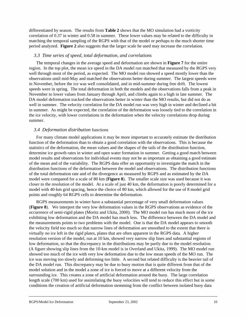
The mean of the total deformation in winter decreased slowly with the size of the area over whiwas calculated (Figure 2) while the correlations between the RGPS measurements and the modelestimates increased. However, the velocity correlation was not strongly dependent on the scale bethese scales are small compared to the autocorrelation length scale of the ice velocity (about 700 kSince deformation events are often highly localized, the improvement in the correlation with increasscale may be due, in part, to mislocations of deformation events in the model. With spatial averagithese mislocations are less significant in reducing the correlation. Because the correlations were b320 km, we concentrate on that scale in most of the rest of the paper.

We begin by reviewing the basic statistics of the velocity and deformation rate as measured on aof 320 km by the RGPS and as estimated by the model without (MO) and with data assimilation (DIn winter (November through May) there were a total of N = 86,664 observation pairs and in summ


acing is

ns of

ter but

nt witheds of DA

e thereheatesstingly,

d to inn than

ated set.

arehileble 2,t ofany

sure 4eealong

uctionces the

er than

ation that thanation.

(1986, daily

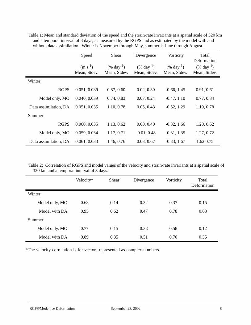
(June through August) a total of N = 29,657. These are not independent samples because their spthe same as the model grid, 40 km, even though the spatial scale of the velocity averages and thedeformation determinations is 320 km. The mean and standard deviation over all times and locatiothe ice speed and the four invariants of the deformation rate are shown inTable 1 for winter andsummer. The correlation values for the velocity and the deformation rates are shown inTable 2.

3.1 Mean ice velocity comparisons

The mean speed of the ice, as measured by the RGPS, was a little higher in summer than in winthe variability is a little lower. The MO simulation had lower winter mean ice speeds than found byRGPS while the DA simulations showed a much better match to the observations. This is consistethe findings of Z2002 in comparisons with unassimilated buoys. However, in summer the mean speboth model runs matched the observations quite well. The velocity correlation was excellent for therun in winter. This is no surprise, since the tracking accuracy of the RGPS is excellent and becausare sufficient buoys within the autocorrelation length scale of most comparison points to constrain tmodel velocity to be near the true ice velocity. Furthermore, the high correlation in the winter indicthat the alignment techniques used to compare these very different data sets were effective. Interethe correlation with data assimilation was diminished from winter to summer, but without dataassimilation it improved. The diminished correlation in summer for the DA simulation may be relatethe loss of the SSMI ice motion data. For the MO case, the correlation was higher in summer thanwinter because the winter model pack was more locked up, with lower mean speed and deformatioobserved, while in summer the MO speed matched the observed speed quite well. The velocitycorrelations for both the MO and the DA runs were somewhat higher than found for daily unassimilbuoy motions by Z2002; the likely reason is the temporal and spatial smoothing applied to this data

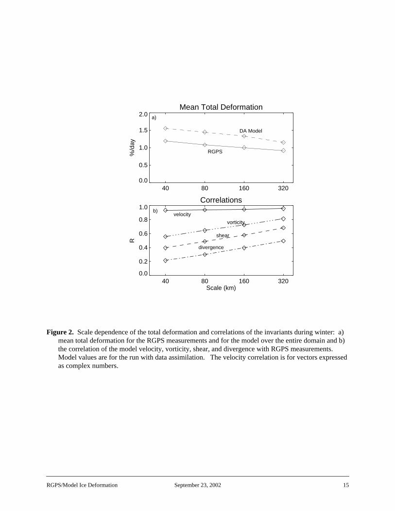
The spatial patterns of the velocity correlation for the MO and the DA runs, winter and summer,shown in Figure 3. The model with no data assimilation showed lower correlations in all regions, wthe model including data assimilation showed markedly increased correlations. As also seen in Tathe velocity correlation for the MO run increased substantially in summer but was still less than thathe DA run, which decreased from winter values. The DA correlation was highest in regions with mbuoy reports available for assimilation. The maximum isR= 0.98, showing that the velocity comparisoncan be excellent where the model is forced to match the ice motion as measured by the buoys. Figshows a map of the total number of daily buoy velocity observations used for assimilation. The largnumber of observations in the Beaufort Sea is related to the SHEBA field experiment. However, thcorrelation remained good even in many regions where there were few buoy observations, except the coasts in summer. In the summer the maximum correlation wasR = 0.88, indicating more difficultyassimilating buoy data in the summer, a result also seen in Z2002 with just the buoy data. The redin correlation along the coasts may have been due, in part, to the assimilation scheme, which reduinfluence of the observations within 200 km of land. Another additional cause could be the model’sincorrect accounting of the shear stresses near the coast.

3.2 Deformation rate comparisons

The deformation rate, as seen in the mean shear or the total deformation, was larger in summin winter. The vorticity showed the largest variability of the deformation invariants in both seasons.There was net anticyclonic rotation. In winter the MO simulation underestimated and the DA simulover estimated the total deformation. Again, this is because the MO simulation had a mean speedwas too low. In summer the mean total deformation was substantially better for the MO simulationfor the DA simulation, although the correlation, while small, was somewhat better for the DA simul

The deformation rates found here are somewhat smaller than the values reported by ThorndikeTable 5) for the AIDJEX array of buoys. He reports a length scale for the array of 800 km and uses


*

f 320 km and

l scale of

The velocity correlation is for vectors represented as complex numbers.

Table 1: Mean and standard deviation of the speed and the strain-rate invariants at a spatial scale oand a temporal interval of 3 days, as measured by the RGPS and as estimated by the model withwithout data assimilation. Winter is November through May, summer is June through August.

Speed

(m s-1)Mean, Stdev.

Shear

(% day-1)Mean, Stdev.

Divergence


Vorticity


TotalDeformation


Winter:

RGPS 0.051, 0.039 0.87, 0.60 0.02, 0.30 -0.66, 1.45 0.91, 0.61

Model only, MO 0.040, 0.039 0.74, 0.83 0.07, 0.24 -0.47, 1.10 0.77, 0.84

Data assimilation, DA 0.051, 0.035 1.10, 0.78 0.05, 0.43 -0.52, 1.29 1.19, 0.78

Summer:

RGPS 0.060, 0.035 1.13, 0.62 0.00, 0.40 -0.32, 1.66 1.20, 0.62

Model only, MO 0.059, 0.034 1.17, 0.71 -0.01, 0.48 -0.31, 1.35 1.27, 0.72

Data assimilation, DA 0.061, 0.033 1.46, 0.76 0.03, 0.67 -0.33, 1.67 1.62 0.75

Table 2: Correlation of RGPS and model values of the velocity and strain-rate invariants at a spatia320 km and a temporal interval of 3 days.

Velocity* Shear Divergence Vorticity TotalDeformation

Winter:

Model only, MO 0.63 0.14 0.32 0.37 0.15

Model with DA 0.95 0.62 0.47 0.78 0.63

Summer:

Model only, MO 0.77 0.15 0.38 0.58 0.12

Model with DA 0.89 0.35 0.51 0.70 0.35


ta but

is is

f theanterAe

ofont for

e

ast

an inpt in

st in thements,

runsns,many

even

mentched

han intion was

inns

d thehisith at

buoy velocities to find mean shear values of 1.0% day–1 for winter and 1.6% day–1 for summer, compared

with the present results from the 320-km 3-day RGPS data of 0.87% day–1 for winter and 1.13% day–1 forsummer. The smaller values found here could be due to the longer averaging time in the RGPS dacould also be a result of sampling different years and different regions.

Of the different measures of the deformation rate, the correlation was highest for the vorticity. Thbecause the standard deviation of the vorticity was largest (Table 1) and because large-scale solid-bodyrotation, which can be well represented by a wind-driven model, contributed a significant amount ovorticity variability. In winter, the correlations were markedly higher for model runs that include datassimilation, as would be expected. The summer DA model run showed lower correlations than wiand there was not as much improvement in the summer correlations of the DA over the MO runs. possible reason is that in winter the coasts and a few buoy motions put significant constraints on thdeformation, while in summer, when the ice pack is nearly in free drift, a few buoy motions do notconstrain the deformation significantly. Also, the summer DA model run did not include the benefitthe SSMI ice motion measurements, which, even with their large error variances, aid the deformatiestimates in winter. Interestingly, in summer the correlation for the divergence was higher than thathe total deformation or shear.

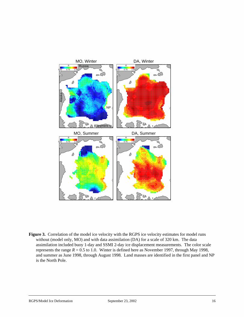
In winter the mean total deformation measured by RGPS for a scale of 320 km was largest in thBeaufort Sea and smallest near the pole (Figure 5). In summer there were broad regions of highdeformation in the central Arctic Ocean and a region of small deformation, perhaps fast ice, in the E

Siberian Sea. Recall fromTable 1 that mean total deformation was 0.91% day–1 in winter and 1.20%

day–1 in summer. The mean total deformation for the MO and the DA runs was larger in summer thwinter as in the observations. The MO run resulted in much lower deformation than the DA run excea few coastal regions. In both winter cases the deformation was largest near the coasts and smallecentral region of the ocean. The deformation for the DA run was larger than in the RGPS measureparticularly near the coasts (for example in the East Siberian Sea and off Point Barrow), and duringsummer.

Maps of the correlation between the observed total deformation and that in the MO and the DAare shown inFigure 6. The correlation was very poor for the MO run at all locations and in both seasobut quite good for the DA run, particularly during winter, far from the coasts, and where there were buoys available for assimilation (Figure 4). The maximum correlation wasR = 0.87. This value isperhaps a good indicator of the best comparison possible between the two very different data sets when the model is constrained to follow the buoy-observed ice motion. The improvement thatassimilation caused in the winter correlation is expected but in summer there was no such improveover much of the region. Both had poor overall correlations, however locally the DA simulation reaR values of 0.84 in the vicinity of the SHEBA camp where many buoys were available, similar to themaximum value in winter.

The winter deformation, both in the observations and in the model, was greater near the coasts tthe interior, while the correlations of both velocity and deformation were lower. This larger deformais undoubtedly due to the constraints the land puts on the ice motion. Because coastal deformationlarger, open water formation, ridging, and ice production rates were also larger in these regions.However, these are just the regions where the correlation was greatly diminished.

Thomas (1999) found correlations between the deformation of 627 buoy clusters 400 to 600 kmdiameter and a number of different model formulations over a 5-year period. The highest correlatiowere for the vorticity, and the correlations for the shear were lower than for the divergence. He founhighest correlation for a simple best-fit linear model of the ice velocity and the geostrophic wind. Tmodel had a vorticity correlation of 0.78. Model formulations very similar to those used here (but wgrid size of 160 km instead of 40 km) showed vorticity correlations of about 0.67. His results are no


y inr time

S veryn thes weretpeak inThe asbit

ion ing

ution the,tweentimate

thections DA

for aid

f the icel andooth is

s ofion.run The ofhe

nometa

differentiated by season. The results fromTable 2shows that the MO simulation had a vorticitycorrelation of 0.37 in winter and 0.58 in summer. These lower values may be related to the difficultmatching the temporal sampling of the RGPS with that of the model or perhaps to the much shorteperiod analyzed.Figure 2 also suggests that the larger scale he used may increase the correlation.

3.3 Time series of speed, total deformation, and correlations

The temporal changes in the average speed and deformation are shown inFigure 7 for the entireregion. In the top plot, the mean ice speed in the DA model run matched that measured by the RGPwell through most of the period, as expected. The MO model run showed a speed mostly lower thaobservations until mid-May and matched the observations better during summer. The largest speedin November, before the ice was well consolidated, and in mid-summer during free drift. The lowesspeeds were in spring. The total deformation in both the models and the observations falls from a November to lower values from January through April, and climbs again to a high in late summer. DA model deformation tracked the observations better in winter than the MO results, but did not dowell in summer. The velocity correlation for the DA model run was very high in winter and declined ain summer. As might be expected, the correlation of the deformation was loosely tied to the correlatthe ice velocity, with lower correlations in the deformation when the velocity correlations drop durinsummer.

3.4 Deformation distributionfunctions

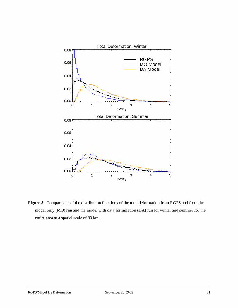
For many climate model applications it may be more important to accurately estimate the distribfunction of the deformation than to obtain a good correlation with the observations. This is becausestatistics of the deformation, the mean values and the shapes of the tails of the distribution functiondetermine ice growth rates in winter and open water formation in summer. Getting a good match bemodel results and observations for individual events may not be as important as obtaining a good esof the mean and of the variability. The RGPS data offer an opportunity to investigate the match in distribution functions of the deformation between the model and observations. The distribution funof the total deformation rate and of the divergence as measured by RGPS and as estimated by themodel were compared for a scale of 80 km (Figure 8). The smaller scale size was used because it wascloser to the resolution of the model. At a scale of just 40 km, the deformation is poorly determinedmodel with 40-km grid spacing, hence the choice of 80 km, which allowed for the use of 8 model grpoints and roughly 64 RGPS cells to determine the deformation.

RGPS measurements in winter have a substantial percentage of very small deformation values(Figure 8). We interpret the very low deformation values in the RGPS observations as evidence ooccurrence of semi-rigid plates (Moritz and Ukita, 2000). The MO model run has much more of theexhibiting low deformation and the DA model has much less. The difference between the DA modethe measurements points to two problems with the model. One is that the DA model appears to smthe velocity field too much so that narrow lines of deformation are smoothed to the extent that therevirtually no ice left in the rigid plates, plates that are often apparent in the RGPS data. A higherresolution version of the model, run at 10 km, showed very narrow slip lines and substantial regionlow deformation, so that the discrepancy in the distributions may be partly due to the model resolut(A figure showing slip lines from the 10-km model is in Overland and Ukita, 1999). The MO model showed too much of the ice with very low deformation due to the low mean speeds of the MO run. ice was moving too slowly and deforming too little. A second but related difficulty is the heavier tailthe DA model run. This discrepancy may be due to buoy motion that is quite different from that of tmodel solution and in the model a zone of ice is forced to move at a different velocity from thesurrounding ice. This creates a zone of artificial deformation around the buoy. The large correlatiolength scale (700 km) used for assimilating the buoy velocities will tend to reduce this effect but in sconditions the creation of artificial deformation stemming from the conflict between isolated buoy da


delrge

n run.

ate of

model

ample of

in

larges cann

veryf thetionso thee

not so

vents,

largeof the found.dds to

belar

erehee that

e therend theures here

and the model field may be inevitable. The incorrect solutions may be the result of errors in the mophysics (or model parameters), the model state (e.g., thickness), or the model forcing fields. The ladifference in the sampling characteristics of the observations and the model results also must beconsidered as a possible source of the discrepancy in the distribution tails.

In summer the model-only run matched the observed distribution better than the data assimilatioUnder summer free drift conditions, when the MO model was no longer locked up (see the speeddistribution plots in Z2002) the impositions of buoy motions appear to add to the deformation estimthe DA model. The correlation of the total deformation also suffered (Figure 7). Even in summer, someof the ice in the observations exhibited near zero deformation while there was almost none in eitherrun.

4. Discussion and conclusions

These comparisons between model-based and observation-based deformation rates are an exhow RGPS data can be used to determine which model formulations provide a better match withobservations. Clearly the data assimilation run provided a better velocity correlation (as expected)winter, but surprisingly in both winter and summer data assimilation did not help with the meandeformation rate and indeed made the total deformation about 20% too large in winter and 40% tooin summer (Table 2). Much of the difference between the model only and the data assimilation runbe traced to the fact that in winter the model-only run has the ice moving 20% too slowly resulting ilower mean total deformation rates.

The correlation between the model estimates and the RGPS measurements of the velocity wasgood, particularly with assimilation of buoy displacement data, throughout the period and in most oregion analyzed, while the correlation in the deformation was much worse. How can velocity correlabe relatively high, but the deformation correlations be relatively low? The deformations are related tspatial derivative of the velocity, and, although the large-scale velocity field is well represented in thmodel (as long as data assimilation is included), the smaller-scale spatial variations in velocity are well represented. Other important factors that can reduce the correlation of the deformation ratescomputed for the model and the measurements include errors in the model location of deformation eand differences determination of the deformation arising from the alignment process. The RGPSdeformation rate measurements may also be biased by excluding cells that have experienced verydeformation. Given the quite different spatial and temporal sampling of the model simulations and RGPS observations, it is perhaps remarkable that the deformation correlations were as high as weThe high correlation of the velocity between the data assimilation run and the RGPS observations athe confidence that can be placed in the analysis and comparison techniques.

Although a high correlation in the deformation is desirable, for many climate applications it maysufficient for ice production estimates if the distribution functions of the deformation rates, in particuthe divergence, are well represented in the model. However our analysis indicates that there wereimportant differences in the distribution functions for both the MO and the DA simulations.

The differences between the observed deformation rates and the DA model deformation rates wparticularly large in the summer. The DA model appears to have larger deformation rates, in both tmean and in the standard deviation and in both shear and divergence. These comparisons indicatsimply assimilating limited quantities of high-quality ice motion data does not insure accuratedeformation rate estimates and can, in some situations, make the estimates worse. However wherwere many buoys to assimilate near the Sheba experiment, the correlation between the observed aDA model deformation was good, showing that with enough ice motion data the assimilation procedcan reproduce the observed deformation. More sophisticated data assimilation schemes than usedmight reduce this problem.


hates of

ionnsanyspectsto the

lationeaneded theange

thercingons

a usefuld. We

d out alutionation.

Jetienceful and

uary

SAR.

f

tion

These comparisons are most useful in showing aspects of the model that need improvement. Wcan these comparisons tell us about the model physics? Many factors influence the model estimatthe deformation rates: wind forcing fields, ocean currents, air and water drag formulations, the icethickness distribution, ice redistribution formulations, and model constitutive laws relating deformatrates to stress. The ice thickness distribution is built up over time, so the thermodynamic formulatiorelating to ice growth and melt also are significant. As a consequence of the interdependence of mmodel units, one cannot change just one element of the model without seeing reflections in many aof the model response. One possibility is to focus on the aspect of the model most closely related deformation: the constitutive law that relates strain rates to stress. Different constitutive laws willproduce different model deformation rates. Which law provides the best fit with the observations?

As an example of the way the RGPS data might be used to this end, we performed a model simuwith the ice strength reduced by 25%. In this simulation no data assimilation was included. The mspeed of the ice increased 28% and the mean total deformation rate increased 24% and both exceRGPS-measured ice speed and deformation. The velocity and deformation correlations did not chsignificantly. The ice thickness over the five-year period of 1993 through 1997, when compared tosubmarine-measured ice draft as in Z2002, showed no change in the bias and a small reduction incorrelation. The best model ice strength depends on many elements of the model, including the fowind field and the wind drag coefficients used. In this case, the deformation and velocity comparissuggest the best ice strength value to be about 20% smaller than in our standard simulation.

The RGPS data set provides highly accurate deformation rate measurements that can provide comparison data set for sea ice models when the two data sets are properly interpolated and alignehave not exhausted the possibilities of using the data to improve our sea ice model, but have pointedirection that we or others can follow. The deformation of the ice plays an essential role in the evoof the ice cover and models will serve us best if they can accurately reproduce the observed deform

ACKNOWLEDGEMENTS

The RGPS and SSMI ice motion data were provided by the Polar Remote Sensing Group at thePropulsion Laboratory, and the buoy data by the International Arctic Buoy Program at the Polar ScCenter, University of Washington. The authors also would like to thank the reviewers for their helpcomments. This study was supported by NASA Cryospheric Sciences Program Grant NAG5-9334ONR High Latitude Dynamics Program Grant N00014-99-1-0742.

REFERENCES

Colony, R.L., and I.G. Rigor. 1993. International Arctic Ocean Buoy Program Data Report for 1 Jan1992 – 31 December 1992,APL-UW TM 29-93. Applied Physics Laboratory, University of Washing-ton, Seattle, 215 pp.

Fily, M. and D.A. Rothrock. 1990. Opening and closing of sea ice leads: Digital measurements fromJ. Geophys. Res.,95(C1), 789-796.

Flato, G.M., and W.D. Hibler, III. 1995. Ridging and strength in modeling the thickness distribution oArctic sea ice.J. Geophys. Res., 100, 18,611–18,626.

Hibler, W. D. III. 1979. A dynamic thermodynamic sea ice model,J. Phys. Oceanogr.,9, 815–846.

Hibler, W. D. III, and K. Bryan. 1987. A diagnostic ice-ocean model.J. Phys. Oceanogr., 7, 987–1015.

Kwok, R., D.A. Rothrock, H.L. Stern, and G.F. Cunningham. 1995. Determination of the age distribuof sea ice from Lagrangian observations of ice motion.IEEE Trans. Geos. Rem. Sens., 33, No. 2, 392-400.


one:

ellite

a Ice

d ice

tic

the

cs,

ith-

ween

Kwok, R. 1998. The RADARSAT Geophysical Processor System. In:Analysis of SAR Data of the PolarOceans, C. Tsatsoulis and R. Kwok, eds., Springer-Verlag, Berlin, 235-257.

Kwok, R., G. F. Cunningham, and S. Yueh. 1999. Area balance of the Arctic Ocean perennial ice zOctober 1996 to April 1997.J. Geophys. Res., 104, 25,747-25,759.

Kwok, R., A. Schweiger, D. A. Rothrock, S. Pang, and C. Kottmeier. 1998. Sea ice motion from satpassive microwave imagery assessed with ERS SAR and buoy motions,J. Geophys. Res., 103, 8191–8214.

Lindsay, R. W., and H. Stern. 2002. The RADARSAT Geophysical Processor System: Quality of SeTrajectory and Deformation Estimates,J. Atmos. Ocean. Tech., submitted.

Meier, W. N., J. A. Maslanik, C. W. Fowler. 2000. Error analysis and assimilation of remotely sensemotion within an Arctic sea ice model. J. Geophys. Res.,105(C2), 3,339–3,356.

Moritz, R.E., and J. Ukita. 2000. Geometry and the deformation of pack ice, Part I: A simple kinemamodel,Ann. Glaciol., 31, 313-322.

Parkinson, C.L., and W.M. Washington. 1979. A large-scale numerical model of sea ice,J. Geophys. Res.,84, 311–337.

Perovich, D. K. and many others. 1999. Year on ice gives climate insights.EOS, 80, 481–486.

Overland, J. and J. Ukita. 1999. Dynamics of arctic sea ice discussed at workshop.EOS, 80, 309–314.

Rigor, I. G., R. L. Colony, and S. Martin. 2000. Variations in surface air temperature observations inArctic, 1979–97.J. Climate, 13, 896–914.

Thomas, D. 1999. The quality of sea ice velocity estimates,J. Geophys. Res., 104, 13,627–13,652.

Thorndike, A. S. 1986. Kinematics of sea ice. InThe Geophysics of Sea Ice, N. Untersteiner, ed., NewYork, Plenum Press, 489-549.

Thorndike, A. S. and R. Colony. 1980.Arctic Ocean Buoy Program Data Report. 19 January 1979 – 31December 1979, Applied Physics Laboratory, University of Washington, Seattle WA, 131pp.

Winton, M. 2000. A reformulated three-layer sea ice model.J. Atmos. Ocean. Tech.,17, 525–531.

Zhang, J., and W.D. Hibler III. 1997. On an efficient numerical method for modeling sea ice dynamiJ.Geophys. Res., 102, 8691–8702.

Zhang, J., W.D. Hibler III, M. Steele, and D.A. Rothrock. 1998. Arctic ice-ocean modeling with and wout climate restoring.J. Phys. Oceanogr.,28, 191–217.

Zhang, J., D.A. Rothrock, and M. Steele. 2000. Recent changes in Arctic sea ice: The interplay betice dynamics and thermodynamics,J. Climate, 13, 3099–3114.

Zhang, J., D. Thomas, D. A. Rothrock, R. W. Lindsay, Y. Yu, and R. Kwok. 2002. Assimilation of icemotion observations and comparisons with submarine ice thickness data.J. Geophys. Res., in press.


, b)d

Figure 1. Illustration of the resampling process for a sample time series at a single fixed 40-km gridpoint over a 50-day period: a) the RGPS sample times showing cells moving through the regionthe daily RGPS and the daily smoothed modelu component of the ice velocity, and c) the resampleRGPS and modelu component. The model results are from the data assimilation model run.

Cell Sample Times

0 10 20 30 40 500

20

40

60

80

100

Cel

l Num

ber

U Component, Daily

0 10 20 30 40 50-5

0

5

10

15

km/d

ay

RGPS Model

U Component, Resampled

0 10 20 30 40 50Days

-5

0

5

10

km/d

ay

a)

b)

c)


r: a)and b).

essed

Figure 2. Scale dependence of the total deformation and correlations of the invariants during wintemean total deformation for the RGPS measurements and for the model over the entire domain the correlation of the model velocity, vorticity, shear, and divergence with RGPS measurementsModel values are for the run with data assimilation. The velocity correlation is for vectors expras complex numbers.

Mean Total Deformation

40 80 160 320

0.0

0.5

1.0

1.5

2.0

%/d

ay

Correlations

40 80 160 320Scale (km)

0.0

0.2

0.4

0.6

0.8

1.0

R

RGPS

DA Model

velocity

vorticity

divergence

shear

a)

b)


scale,nd NP

Figure 3. Correlation of the model ice velocity with the RGPS ice velocity estimates for model runswithout (model only, MO) and with data assimilation (DA) for a scale of 320 km. The dataassimilation included buoy 1-day and SSMI 2-day ice displacement measurements. The color represents the rangeR = 0.5 to 1.0. Winter is defined here as November 1997, through May 1998and summer as June 1998, through August 1998. Land masses are identified in the first panel ais the North Pole.

MO, WinterR

0.50 1.000.75

DA, WinterR

0.50 1.000.75

MO, SummerR

0.50 1.000.75

DA, SummerR

0.50 1.000.75

Russia

Ellesmere Is.

Ala

ska

NP


yed in
Figure 4. Number of daily buoy observations in each 40-km grid square during the 10-month study
period. The concentration of observations in the Beaufort Sea is largely due to the buoys deplothe vicinity of the drifting SHEBA ice camp. The trajectory of the ice camp is shown in black.

Number of Buoy ObservationsN

0 50 25


the.

Figure 5. Mean total deformation rate estimated by RGPS observations, the model only (MO), andmodel with data assimilation (DA) at a spatial scale of 320 km and a temporal interval of 3 days

MO Winter%/day

0.0 2.0 1.0

DA Winter%/day

0.0 2.0 1.0

MO Summer%/day

0.0 2.0 1.0

DA Summer%/day

0.0 2.0 1.0

RGPS Winter%/day

0.0 2.0 1.0

RGPS Summer%/day

0.0 2.0 1.0


therval

Figure 6. The correlation between the total deformation measured by RGPS and that estimated bymodel only (MO) and with data assimilation (DA) at a spatial scale of 320 km and a temporal inteof 3 days. The color scale represents the rangeR = 0.0 to 1.0.

MO, WinterR

0.0 1.0 0.5

DA, WinterR

0.0 1.0 0.5

MO, SummerR

0.0 1.0 0.5

DA, SummerR

0.0 1.0 0.5


locitydows

Figure 7. Time series for the RGPS (black line) and the model (both model only, MO, blue line, andwith data assimilation, DA, orange line) of the mean speed, the mean total deformation, the vecorrelations, and the total deformation correlations. The statistics are computed for 10-day winevery 5 days over the entire domain for the 320-km scale estimates.

Mean Speed

350 400 450 500 550 6000.00

0.02

0.04

0.06

0.08

0.10

m/s

Total Deformation

350 400 450 500 550 6000.0

0.5

1.0

1.5

2.0

2.5

%/d

ay

Velocity Correlation

350 400 450 500 550 6000.0

0.2

0.4

0.6

0.8

1.0

R

Total Deformation Correlation

350 400 450 500 550 600Days

-0.2

0.0

0.2

0.4

0.6

0.8

1.0

R

Nov Dec Jan Feb Mar Apr May Jun Jul Aug

RGPS

RGPS

Days

MO

MO

DA

DA

MO

DA

MO

DA


e

he

Figure 8. Comparisons of the distribution functions of the total deformation from RGPS and from th

model only (MO) run and the model with data assimilation (DA) run for winter and summer for t

entire area at a spatial scale of 80 km.

Total Deformation, Winter

0 1 2 3 4 5%/day

0.00

0.02

0.04

0.06

0.08

RGPS MO Model DA Model

Total Deformation, Summer

0 1 2 3 4 5%/day

0.00

0.02

0.04

0.06

0.08


rgps model deformation

Documents