rights / license: research collection in copyright - non ...40074/... · tableofcontents...
TRANSCRIPT

Research Collection
Doctoral Thesis
Fast, accurate and robust estimation of mobile robot position andorientation
Author(s): Vestli, Sjur Jonas
Publication Date: 1995
Permanent Link: https://doi.org/10.3929/ethz-a-001545321
Rights / License: In Copyright - Non-Commercial Use Permitted
This page was generated automatically upon download from the ETH Zurich Research Collection. For moreinformation please consult the Terms of use.
ETH Library

25. Jan. 1996DISS. ETH No.: 11360
Fast, accurate and robust estimation of
mobile robot position and orientation
A dissertation submitted to the
SWISS FEDERAL INSTITUTE OF TECHNOLOGY
ZURICH
for the degree of
Doctor of Technical Sciences
presented by
Sjur Jonas Vestli
M.Sc, B.Sc. University of Salford, UK
Sivilingeni0r, Norges Tekniske H0yskole Trondheim (NTH), N
born 30. June 1964
citizen of Norway
accepted on the recommendation of
Prof. Dr. G. Schweitzer, examiner
Prof. Dr. E. von Puttkamer, co-examiner
1995
Acknowledgements
This thesis is based on research performed at the Institute of
Robotics of the ETH Zurich between 1991 and 1995.
I would like to thank my supervisor, Professor Dr. G. Schweitzer,
for making this whole thing possible and for providing guidance
during the course of this work. I would also like to thank Professor Dr.
E. von Puttkamer for his valuable comments and for accepting to be
my co-examiner. Many thanks are also due to all those of you who
helped me throughout the realisation of this work. I also wish to
express my gratitude towards the Royal Norwegian Council for
Scientific and Industrial Research (NF / NTNF) for their financial
support during the first three years.
Zurich, December 1995 Sjur Jonas Vestli

Table of contents
Table of contents i
Abstract v
Kurzfassung vii
1 Introduction 1
1.1 Synopsis 1
1.2 Motivation 2
1.2.1 General motivation 2
1.2.2 Need for mobile robot localisation 3
1.3 Summary of existing position update methods 4
1.4 Objectives 7
1.5 Approaches 7
2 State of the art 9
2.1 Problem statement 9
2.2 Methods of mobile robot localisation 10
2.2.1 Occupancy grid-based representations and
localisation 11
2.2.2 Sonar based localisation in
object based maps 13
2.2.3 Matching and clustering 16

11
2.2.4 Optical rangefinder localisation in
object based maps 18
2.2.5 Crosscorrelation of sensor scans 21
2.2.6 Topological representations and localisation 22
2.2.7 Special systems 23
2.3 Discussion 24
3 Mobile robot positioning 27
3.1 Guide to this chapter 27
3.2 General requirements 27
3.2.1 Test for position update systems 29
3.3 Matching sensed to modelled geometric features 31
3.3.1 World modelling 31
3.3.2 Range sensing 32
Ultrasonics 33
Optical coaxial systems 35
Optical triangulation systems 36
Solution to our problems 37
3.4 Preprocessing 39
3.5 Compression / simplified formulation 44
3.5.1 Position from a wall 44
3.5.2 Extraction of straight lines 48
3.5.3 Cluster analysis 52
3.5.4 Position from a corner 62
3.5.5 Extracting corners 64
3.5.6 Position from a cylinder 67
3.5.7 Summary of structure extraction methods 72
3.5.8 Combination of different
geometric information 74
3.6 Scanning while moving 77
4 Experiments 81

Ill
4.1 Guide to this chapter 81
4.2 Test for real time performance 81
4.3 Test for repeatability 85
4.4 Test for robustness 88
4.5 Positioning from corners 92
4.6 Overall performance 97
4.7 Scanning while moving 100
4.8 Discussion 101
5 The robot 103
5.1 Guide to this chapter 103
5.2 The mobile platform 103
5.3 Scanning laser range finder 107
5.4 Robot controller 110
6 Conclusions 113
6.1 Guide to this chapter 113
6.2 Mobile robot positioning,problems and requirements 113
6.3 Discussion of thesis 114
6.4 Contributions 117
6.4.1 Prefiltering 117
6.4.2 Abstraction level 117
6.4.3 Transformation of sensor data 118
6.4.4 Extraction of features 118
6.4.5 Equation for position 119
6.4.6 Performance and performance measure 119
6.4.7 Summary 120
6.5 Outlook 120
6.5.1 Reducing processing time 120
6.5.2 Increasing accuracy 122
6.5.3 Extension of the method 123
iv
6.5.4 Odometry calibration 124
6.5.5 Speculative clustering & map-building 124
6.5.6 Fusion with ultrasonic data 124
6.6 Summary 125
References 127

Abstract
This work is an investigation into methods of mobile robot
localisation. New robust and real time capable methods are introduced
and analysed before being tested on a mobile robot platform. The
algorithms introduced use noisy range data and a world model to
achieve localisation. Significant effort is put into achieving acceptable
performance in the presence of sensor noise, and a number of filtering
techniques for range data are described. A mobile robot platform,
designed for demanding indoor use, is used for performance testing of
the methods. Several thorough demonstrations of these methods in
typical operating environment of the mobile robot (i.e office type
buildings) are described. Suggestions for further improvement on these
methods and the related techniques are provided.

vi
Vll
Kurzfassung
Diese Arbeit ist eine Untersuchung tiber die Methoden der
Positionsbestimmung von mobilen Robotern. Neue, robuste und
echtzeitfahige Methoden werden eingefiihrt und analysiert, bevor sie
auf einer mobilen Plattform getestet werden. Die entwickelten
Algorithmen verwenden verrauschte Entfernungsmessungen und ein
Weltmodell, urn die Position des Fahrzeuges zu bestimmen.
Erheblicher Aufwand wurde zum Erreichen einer akzeptablen Leistung
bei vorhandenem Sensorrauschen betrieben. Dazu werden
Filtertechniken fur die Distanzmessungen beschrieben. Die Leistung
der Algorithmen wird anhand einer mobilen Plattform getestet, die fur
Anwendungen in Gebauden bestimmt ist. Mehrere Beispiele dieser
Methoden in typischen Umgebungen des mobilen Roboters (z.B.
Biirogebaude) werden eingehend beschrieben und diskutiert. Am
Schluss werden Vorschlage fur weitere Verbesserungen dieser
Methoden und der damit verbundenen Techniken aufgefiihrt.

viii

1
1 Introduction
1.1 Synopsis
The objective of this thesis is to realise new, fast, accurate and
robust methods for mobile robot localisation. After an investigationinto existing methods and the development of new and improvedmethods a demonstration of the viability of these new techniques will
be performed on a mobile robot test bed.
Chapter 1 will outline why mobile robots and localisation of
mobile robots are an issue and why this work was seen as necessary.
Chapter 2 will provide a review of the state of the art with respect to
localisation methods of mobile robots. In Chapter 3 new algorithmsthat can alleviate some of the existing problems will be presented, in
particular how it is possible to achieve real-time performance,
accuracy and robustness with one method. The performance of these
new methods are described in Chapter 4. Chapter 5 presents the mobile
robot experimental platform and sensor system, and explains how the
position update methods are integrated with the rest of the control
software. Chapter 6 rounds off this thesis with conclusions, summaryand recommendations for further work.

2
12 Motivation
1.2.1 General motivation
There is a trend to enhance the capabilities of robotic devices
which is supported by the ready availability of computer power and
sensor systems. The main perceived benefits are increased efficiency of
the production line, lower labour costs, etc. all of which give the
owners more return from the money invested. In some cases an
additional benefit comes from the fact that previously impractical
applications can be addressed. Taking the particular example of mobile
robots or autonomous guided vehicles1 several examples can be
observed where the above mentioned benefits have been achieved, in
particular:
The Helpmate from Transitions Research Corporation used
for service tasks in several U.S. hospitals,The K2A from Cybermotion for security inspection used at
the Los Angeles museum of art.
There are also reasons for using robot systems not based solely on
financial arguments, for instance:
Recovery operations after chemical, nuclear or fire accidents,
Handling hazardous substances,
Mine clearance.
The above are typified by the fact that the tasks are dangerous to
humans. Indeed robots are already in use for a number of such tasks,
for instance in handling radioactive samples (plenary talk IEEE
Conference on Robotics and Automation 1993) and in the Chernobyldebris clearance operations.
1. Both mobile robots and autonomous guided vehicles (AGVs) are machines that
move freely around, as opposed to robot manipulators. The difference between an AGV
and a mobile robot lies in that where as an AGV need some sort of installation to
navigate, e.g. an inductive wire in the floor to follow, a mobile robot is independent ofsuch installations.

3
Unfortunately it has been impossible or difficult to use robots for
all such applications. There are several reasons for these shortcomings.The problem is that the current generation of "autonomous robots" are
not sufficiently autonomous and must be teleoperated. Unfortunately,in most cases only a limited amount of transmitted video information is
available, therefore teleoperation turns out to be a very strenuous task
[Jashmidi 93]. An overview of the current state of the art of robotics in
hazardous environments can be found in [Jashmidi 93] and [Fogle 93],
[Fogle 93] details the usage of mobile robotic devices in particular.
It is thus natural to try to increase the level of autonomy,
capability and thus the required "intelligence" of robot systems. This
thesis is a contribution to this endeavour in that the methods described
here enable a mobile robot to frequently calculate its absolute positionwithin a building. Furthermore, the absolute position is known with a
high degree of accuracy for extended periods of operation in the
presence of sensor noise and obstacles.
This then enables more autonomous navigation than currently
possible through alleviating some of the burdens normally placed on
an operator. It is viable to use mobile robots for a wider range of
applications where extensive human assistance as provided during
teleoperation is either difficult or unwanted.
In addition to the disaster scenarios above this also opens up the
possibility of using mobile robots for such tasks as mail distribution in
office buildings. These tasks could previously not be automated with a
robot system, since the necessity of teleoperation of the system
provided no gain.
1.22 Need for mobile robot localisation
Of course calculating the mobile robots position is not a new
problem. In fact the problem is not limited to mobile robots. Imaginethat you have to row across a lake from your boat house to a colleague
on the other side in thick fog. You know your start point (your boat
house) and how long and in what direction you have to row to reach

4
your colleague. But if you try you will probably fail, because you don't
know exactly how many metres you row per stroke, and maybe your
compass had a small offset in it. The same problem is experienced on
the open sea, where there is no absolute reference point to aid the
calculation of position. Historically the stars in the sky and the heightof the sun (at noon) were used to gain such an absolute reference.
Nowadays we can rely upon satellite (GPS) and radio navigationbeacon aids to locate to an accuracy of a few metres anywhere on the
earths surface. Most mobile robots though still operate using methods
very similar to those of the rower above. They measure their wheel
revolutions and incrementally try to estimate their position, and
unfortunately for (most) mobile robots GPS systems do not work
indoors, and re-creating such referencing systems with beacons is
usually infeasible.
Humans, however, have few problems in navigation in buildingsbecause we use our excellent visual capacity to stop in front of the
office which we intended to reach, or in the case of blindness (or
darkness) we use tactile sensing to detect enough features to localise.
Similar information is normally available to a mobile robot, either in
the form of a range sensor system or as gray level images. Trying to
localise using such information has been addressed a number of times
in the literature and many methods have been proposed. This work will
investigate the merits of these various approaches and it will also
propose new methods. The viability of these new methods will be
demonstrated, in particular it will focus on:
Real time capability
Requirements on the robot platform and sensors
Reliability of the methods
Accuracy of the methods
13 Summary ofexisting position update methods
In chapter 2 a thorough literature review will be undertaken,
however, it might be useful to provide some "advance information"

5
here. In table 1 below a summary of the reviewed position update
methods is presented.
One of the main drawbacks of all these methods is the
unacceptable processing times demanded. The last column of table 1
details the maximum CPU time required in order to calculate the
position of the robot, ignoring the time required to record the sensor
data on which the calculation is based. There is only one which
approaches real time performance, however this was achieved by
sacrificing accuracy. The methods which use a point to structure
matching (range-reading to world-model matching) are all extremelyCPU intensive. This becomes clear when the methods are analysed
(see chapter 2) because large over-determined systems of equationshave to be solved. In addition, it is necessary to invest significant effort
into the matching process, and the time needed increases linearly with
both the size of the world model and the number of range readings.
Among those authors who use ultrasonic range data for positioning a
tendency to use structure to structure matching is found. This is
motivated by the particular characteristics of ultrasound sensor
systems. In polar scans ultrasound sensors tend to generate Regions of
Constant Depth (RCD) where walls, corners, etc. are present. Thus an
RCD is evidence for the presence of a structure in the environment1.
After an RCD extraction process a structure to structure matching is
performed. Generally structure to structure matching produces systems
of lower complexity than the point to structure matching. The cost is
that more preprocessing is necessary. Generally even simpler and more
robust methods are needed to achieve the required real-time and
accuracy performance.
/. This characteristic also means that any ultrasonic range reading which is not amember ofa Region of Constant Depth is virtually useless.

methods
update
posi
tion
reviewed
of
Summary
1.Table
Unknown
Unknown
Various
Ultrasound
Schiele
updates
for
seconds
0.5
-0.2
mate,
esti
¬in
itia
lfor
seconds
5°
2/
cm
2-3
sens
ing
Directed
Ultrasound
Holenstein
seconds
10
°
3/
cm
1
matchingstructure
to
Point
Ultrasound
MacKenzie
second
1°
2.5
/cm
5
filt
er
Kalman
+RCDs
Ultrasound
Leonard
seconds
0.2
°
0.5
/cm
5
scans
of
Convolution
scanner
Opti
cal
WeiB
larg
e)(suspected
Unknown
unknown
cm/
3
matchingstructure
to
Point
scanner
Radar
RuG
seconds
8
unknown
cm/
1
matchingstructure
to
Point
scanner
Opti
cal
Cox
required
time
CPU
typi
cal
Accuracy
Method
system
Sensor
author
Principa
l

7
1.4 Objectives
Inspecting table 1 it becomes clear that improvements are
necessary for operation of mobile robots without the introduction of
artificial landmarks (introduction of such removes the whole problem,at the cost of modifying the environment). Essentially the only method
that approaches real time capability is that of WeiB from the
Universitat Kaiserslautern (0.2 seconds), however, this particular
work, provides the least accuracy.
The goal is therefore to produce a 2-dimensional 3-degree-of-freedom position update system that is:
fast (<1 second for a position update)
accurate to (at least) 1 cm and 0.5°
tolerant towards unmodelled obstacles.
1.5 Approaches
Chapter 3 will, in detail, present new methods for calculating the
position of a mobile robot based on range data from the environment.
However, for the benefit of the reader, a short overview of the methods
employed for mobile robot positioning will be presented here.
In order to enable completion of a position update cycle within the
prescribed 1 second, a structure to structure matching scheme is
proposed. It will be assumed that structures, such as walls, corners and
cylinders, are present in the robots environment and that the location of
these structures are available in the robots world model, i.e. the
location of the structures are given in the world co-ordinate system.
Furthermore, algorithms will be developed that can extract the
positions of the same structures (walls, corners and cylinders) in the
robots sensor data, i.e. the positions of the structures are found in the
robot co-ordinate system. With the knowledge of the position of a
structure in the world co-ordinate system and in the robot co-ordinate
system, it is possible to set up and solve an equation for the robots
position in the world co-ordinate system. The equation for the robots

8
position is over determined if several structures are considered
simultaneously. However the complexity of the equation for the robots
position will remain moderate since the number of structures visible at
any one time is limited. Due to the relatively low complexity of the
equation for the mobile robots position is it possible to meet the real¬
time requirement.
The range data will initially be preprocessed in order to remove
any erroneous data, and in order to gain a relatively uniform
distribution of range information from the robots immediate
environment. After the preprocessing the data will be processed so that
the location of the walls, corners and cylinders will manifest
themselves as clusters, and so that the co-ordinates of the clusters
provide the position of the corresponding structures in the robot co¬
ordinate system.
In chapter 4 the methods will be thoroughly tested, and it will be
demonstrated that the methods developed in this thesis are accurate
and robust.

9
2 State of the art
2.1 Problem statement
This chapter provides a definition of the problem at hand and a
thorough review of current methods.
For a number of mobile robot applications it is necessary for the
robot to have knowledge of its own relative position in the 3 degree-of-freedom work space. For instance if the work space of the robot is an
office building with corridors, halls and offices and the task of the
robot is to carry a payload from one office (start) to another office
(goal) the robot will need to know:
When it has reached the goal (requirement A)
How to reach the goal starting at the start position(requirement B)
If we assume that the information of the building and the goal is
given in the form of maps containing the layout of the building (other
methods are possible, see section 2.2.6) and the goal is specified as a
point (or small area) in this layout, then the "most natural" way for the
robot to fulfil requirement A (above) is to continuously check if its
current position in the building is close (in the Euclidian sense) to the
given goal. The methods required in order to have an accurate estimate
of the current position continuously available turn out to be a major

10
issue and are the themes of this chapter. The second requirement listed
above (requirement B) is not addressed in this thesis.
Unless specific measures are taken a mobile robot does not
automatically have any knowledge of position. A commonly used
method for calculating the position is to measure the rotation of the
wheels and from this deduce the position through the usage of the
robot's kinematic equations, a method known as odometry or dead
reckoning .This method is always incremental, an initial estimate is
used and the relative motion over a short time interval is added. An
example of the equations behind this incremental method is presentedin section 5.2. Due to this incremental nature it is inevitable that even
small systematic errors such as inaccurate knowledge of the wheel
radii will over time add together and take on unacceptable proportions.An example of the magnitude of the errors introduced over a relativelyshort trajectory is presented in section 4.6. Any method relying solelyon the mobile robot's internal sensors will have the same problems,therefore a method which uses absolute information from the
environment such as the location of artificial beacons or naturally
occurring landmarks is necessary.
2.2 Methods ofmobile robot localisation.
Ever since the early days of mobile robotics this issue has been
addressed. Moravec [Moravec 80] describes a method for the Stanford
cart using multiple camera images from which the 3D position of a
number of features are extracted. These features are matched to the
features recorded at the previous location. From the correlation
between the features detected in the two situations the new robot
location (relative to the old robot location) is calculated. Even after
considering the technical progress particularly in terms of available
1. Dead reckoning is defined by the OED [Simpson 89] as: "The estimation of aship's position from the distance run by the log and the course steered by the compass,with correctionsfor current leeway, etc., but without astronomical observation".

11
computer power the performance of the Stanford cart was not exactly
impressive (up to 5 hours for a total robot movement of 20 m).
Since then a number of authors have addressed the problem of
localisation and a number of different methods have established
themselves. The various alternatives will be discussed below.
2.2.1 Occupancy grid-based representations and localisation
The occupancy-grid is a very popular form for the representationof the environment. Early supporters of this method were Moravec and
Elfes [Elfes 87] and [Moravec 85]. The representation has since been
used by a number of other researchers [Schiele 94], [Courtney 94].
In the simplest of these schemes the environment is mapped onto
a regular grid. Each of the grid cells contains information indicating
occupancy, i.e.whether the particular cell is empty or not. Typicallyvalues between 0 and 1 are used to indicate the status of the cells. As an
example 0 might indicate a 100% certainty that the cell is empty, a 1
might indicate 100% certainty that the cell is occupied, and in between
values indicate some uncertainty about the state of the cell. In figure 1
- Trajectory junction
Figure 1: Left a typical environment where two corridors
intersect, right the occupancy grid representationthereof.
12
a graphical view of an example environment and its corresponding
occupancy grid representation is provided. One of the main benefits
from occupancy grids is the property that statistical sensor range data
can be integrated effectively into a cartesian representation.
In [Elfes 87] a brief overview of the different localisation methods
within occupancy grids that the authors have tested are outlined. An
obvious approach to this is to correlate the local (constructed by sensor
data) map to the reference (a priori) map. This approach is obviously
expensive in terms of CPU time required and the author also reports
that significant portions of an hour on a mainframe computer may be
required. This is obviously impractical.
Noting that only the occupied cells contain information the
authors proceed to extract and label (according to their position) the
occupied cells from both maps and via trial-transformation matrices to
attempt a correlation in a 1 dimensional space. This produces
significant, but still insufficient, speed-ups (processing time down to a
few minutes).
The authors then resort to maintaining hierarchical occupancy
grids with many different resolutions. A localisation is initiated in the
least accurate map and subsequently refined in the maps of higher and
higher resolution. This, together with rejection of high frequency
"occupancy", produces tolerable performance. The authors report an x,
y accuracy of 15 cm and an orientation accuracy of 3° requiring
approximately 1 sec VAX processing time.
In a more recent paper Schiele and Crowley discuss several
techniques for mobile robot positioning with occupancy grids
[Schiele 94]. The authors consider the problem as a matching between
two separate occupancy grids, the local occupancy grid (an occupancy
grid image of the local environment constructed from recent sensor
data) and the global occupancy grid provided from a CAD system or
built by the robot in some way or other. Assuming that an odometric
position estimate is available a correction (or "innovation") is
calculated from the matching process and the updated position is

13
calculated using a Kalman filter framework. The correction and
innovation can be calculated in 4 ways, namely:
1 Correlation of the grids (as used by Moravec and Elfes see
above).
2 Extraction of line segments in both grids using a modified
Hough transform (MHT) algorithm, subsequent matching of
line segments and calculation of an innovation from each and
every line segment.
3 Extraction of line segments in the local grid (with MHT as
above), generation of a mask using these extracted line
segments and a subsequent correlation of the mask and the
global grid. The best correlation yields the innovation.
4 The same as number 3 but the roles of local and global gridreversed.
The authors report the best results from method 2 (extracting and
matching line segments in both grids), however, no exact performancedata is provided. We, however, expect the required CPU time to be
relatively large as the computation of the Hough transformation tends
to be a very costly operation. The accuracy / repeatabilty of these
methods would definitely be a function of the grid size and Houghtransform resolution (finer grid / higher resolution = higher accuracy),on the other hand, decreasing the grid size or increasing the HT
resolution would also require more computational power.
222 Sonar based localisation in object based maps
One of the most thorough investigations into the usage of sonars
for localisation, in a metric sense, was provided by Leonard and
Durrant-Whyte [Leonard 92]. Instead of considering the pure sonar
range readings the authors utilise regions of constant depth (RCDs) of
the sensor scans, since RCDs are more easily matched to modelled
geometric structures. Furthermore an extended Kalman filter algorithmis used for the fusing of the data with the odometric estimate, this has
the further advantage of being able to consider the uncertainties
inherent in the system (odometry, sensor readings, etc.).

14
Due to its nature it is more or less impossible for a sonar to have a
narrow beam and hence well defined angular resolution. Kuc and
Siegel discussed these properties in [Kuc 87]. This means that for
instance corners and walls result in a set of range readings that have a
constant range over a certain range of angles (for a scanning sensor).
Scanning one environment from (slightly) different positions will
result in that a RCD from a wall moves along the wall, and that a RCD
from a corner will stay stationary and rotate. In other words: extractingthe RCDs from successive scans and using the development as a
mobile robot moves allows us to identify the source for the RCD(s)and the location of this source.
Given the old mobile robot position, the last movement, a map of
the building and utilising the above mentioned RCDs and an extended
Kalman filter framework the process for mobile robot positioning is as
follows:
1 Calculate new (odometric) position and error covariance.
2 Get RCDs from the sensor scan at the new position.3 With the predicted position (point 1 above) and the map
predict RCDs and variances.
4 Match the predicted (point 3) and observed (point 2) RCDs.
5 Use data from 1 and 4 (and through 4 also information from
3) update the position, and the variances.
A problem in the procedure sketched above remains the matching
procedure. For the sake of simplicity the authors ignore any RCDs that
report matching problems (no match, several matches, etc.).
The implementation of these algorithms requires approximately 1
second of processor time. It is not reported whether this applies to the
experimental platforms embedded controller (a Motorola 68020
system) or the host computer (Sun3 / Sun4 systems), although we do
not expect the differences to be major. Studying the results presented in
[Leonard 92], a rotational accuracy/repeatabilty of approximately±2.5° and a translational accuracy/repeatabilty ±50 mm is achieved.
Furthermore it is noted that occasionally the algorithms diverge (for

15
instance if an un-modelled object consistently returns RCDs), and that
it is very difficult to tune the filter parameters. This was also verified bystudies at the IfR, ETH [von Flue 94]. Nevertheless, this must certainlybe described as one of the more successful approaches to localisation
with sonars, and maybe one should not expect any higher level of
accuracy and reliability when this sensor modality is the only one
utilised.
In contrast to the usage of RCDs as described above are the
investigations by MacKenzie and Dudek [MacKenzie94a]. Usingultrasonic range data the authors compare clusters of range readings
directly to the modelled environment using a method akin to that of
Cox (see section 2.2.4 and [Cox 90]). After the association stage
(determining the relationships between clustered sensor data and
modelled lines) a correction (transformation) of the position is
calculated and applied to the current (odometric) estimate. The
correction is a weighted sum of contributions from each match
between clusters (sensor data) and modelled lines. The contribution
from each line & cluster is the projection onto the normal of the
modelled line. This procedure must always be applied a number of
times1 before the updated position stabilises. Significant is that since
the algorithm does not rely upon RCDs localisation can be achieved
using one scan from a single position.
This method demonstrates high tolerance against large initial
errors in the (odometric) position estimate. In specific cases the initial
error could be up to 3 m and still the estimate would converge to the
true position within an accuracy of a few cms and degrees. However,
with a small offset in the initial position a divergent behaviour of the
method can be observed. Considering this problem in optimizationterms one can say that the procedure is vulnerable to being trapped in
local minima.
1. This is afunction ofthe initial (odometric) position estimate, if this is good then10 iterations may suffice, if it isfar offmore iterations are needed (approx. 40), these are
typical values only [MacKenzie 94b].

16
The authors recognise this as a problem, and introduce an
independent measure for the quality of the final estimate, the
classification factor Ecf. Ecf is defined as follows:
1" ( d" )
,• = l^ di +c )
where dt is the distance between a sensor reading, i, and the line to
which is was associated, c is a "neighbourhood" size (outlier
measurements outside the neighbourhood are rejected) and m is a
constant indicating the level to which outlier measurements are
ignored. Ecf approaches unity at the true position and is significantlysmaller where local minima are observed, and hence the problem of
local minima can be addressed.
The accuracy (repeatabilty) of these algorithms are in the order of
1 cm for x and y and 3° for the orientation, however, it turns out to be
computationally expensive. The authors report 10 seconds and upwardon high performance RISC workstations (Silicon Graphics Indigo/Indy
@ 100 MHz) [MacKenzie 94b].
223 Matching and clustering
From the research group of E. Badreddin at the ETH an interesting
contribution to position update with ultrasound sensors has been
provided [Holenstein 92]. In his thesis Holenstein chooses to split the
problem into three separate sub-problems, namely those of:
initially (from a stationary position) to determine the positionof the robot without a-priori knowledge
continuously update the position when moving
moving onto a docking station high accuracy positioning.
The latter method introduces artificial landmarks into the
environment and is as such not of interest to us.

17
For the first two sub-problems the author utilises a world model
that contains walls and corners. Furthermore the inherent property of
ultrasound sensors (generation of regions of constant depth) is
exploited.
The problem of localising the robot when stationary and with onlythe world model as a-priori information is the main theme of
Holensteins thesis. Using the reference model (containing the world
co-ordinates of corners and lines) and extracted locations of corners
and lines in the sensor data (more on this extraction process later) the
author considers all possible matches between modelled and sensed
objects. For each and every one of these matches a robot location is
calculated. For all "correct" matches we have more or less the same
robot position and the robot position can be found by cluster analysisin the space of all the possible positions.
The extraction of objects in the sensor data uses much the same
method as discussed by Leonard. However as the robot is stationary
during the process it is more difficult to separate corners from walls.
An attempt to classify the separate RCDs is made using some
heuristics, but the author acknowledges the unreliability of this
approach.
This method provides a rough estimate which is subsequently
improved through matching all the objects simultaneously (using the
rough position) and solving for the improved position with a least
squares method. The formulation of this improvement is such that
corners and walls are treated differently and subsequently combined.
Typically the accuracy of the final estimate is 2-3 cm and 2°.
Typically this process takes about 5 seconds. It is also possible for the
method to fail and heuristics have to be introduced to improverobustness.
For the purpose of updating the position when the robot is movingHolenstein calculates the theoretically visible corners and walls usingthe world model and the odometric position. The theoretically visible

18
objects are used to predict particular sensor values in particular
directions (such as perpendicular to expected walls) and predicted
values are compared with actual sensor values. If the values are within
specific tolerances then the information is combined with the odometry
in a Kalman filter to calculate the position. It is worth noting that the
author must treat the x and y co-ordinates separate from the 8 co¬
ordinate, and that the 8 co-ordinate cannot be updated based on the
environment. Unfortunately the 8 co-ordinate is important for
estimating the expected location of the modelled objects in the sensor
frame, therefore a fibre-optical gyro is used and fused with odometric
position estimate. Typical accuracies achieved are of the order of 5 cm.
One update needs approximately 0.2 - 0.5 seconds CPU time
[Badreddin95].
2.2.4 Optical rangefinder localisation in object based maps
A central contribution to the field of mobile robot localisation was
provided by Ingemar Cox [Cox 90]. In this work a scanning optical
range finder which measures the phase difference of transmitted and
reflected light is used together with a world model composed of
straight lines.
The sensor readings (polar r,8 or cartesian x,y) provided from the
sensor have a noise level of approximately 2.5 cm (1") at a range of 1.5
m (5')- This sensor system is used also by a number of other
researchers and a thorough treatment of the sensor can be found in
[Adams 92]. For each separate sensor reading the nearest modelled
line is found by searching the data-base containing the line model of
the current environment, and the distances between the lines and the
points are calculated. Then a transformation matrix is calculated that
minimises the sum of the squared distances. This procedure is repeated
iteratively until the solution converges. The last step is necessary since
it is possible that a number of the sensor readings are associated to the
"wrong" line in the first step. However, the position estimate improveswith each iteration so that mis-matches are eliminated. At the end the
result is "fused" with the odometric position estimate.

19
This algorithm produces acceptable results with an accuracy of
0.7° in orientation and 3 mm in x and y (0.1"). However the
computational load is rather high with updates of the position every 8
seconds (assuming 180 measurement points and 24 line segments
considered). The real time system being employed is a Motorola 68020
VME system with 1 processor and a real-time operating system
[Cox 90], so the 8 seconds also include processor time allocated to
motor control and other parallel processes.
Cox claims that the algorithm is robust with respect to spuriousdata from un-modelled obstacles or people. This assumes that the
instantaneous position error is small (i.e. frequent updates can be
made), since then data from un-modelled obstacles can be rejected
prior to the matching algorithm. However, Cox recognises that this
assumption may not hold in general. It is also worth noting that the
robot system on which the algorithms are being used have an extra set
of encoder wheels (with no-load) specifically for the purpose of
providing a good odometric position estimate.
Furthermore it would be difficult and computationally expensiveto extend this scheme to 3D - this is also recognised by Cox.
Another group at the Technische Universitat Miinchen have also
been working on methods very similar to those of Cox [RuB 93]. This
group utilises a high frequency (94 GHz) radar sensor for range
sensing. The closest modelled line to the (x,y) range data from this
sensor is found and the vector from the point to the line ([dx, dy] ) in
the world co-ordinate system is calculated using the available
odometric estimate of the robot position ex and ev. The soughtcorrection vector ([Apx, Apy, Ap^] ) for a single point is then (if we
assume a small correction in the angle) given as below in equation 2.
-1 0 -e'y0 -1 ex
*pxd
*Pyax (EQ.2)

20
Combining all the points is equivalent to extending this system of
linear equations as in equation 3 (the second subscript refers to the
measurement point number). This system of equations is then solved
_
-
Jl ° ~eyl *xl
0 -1 exl dyi-1 ° ~ey7
"A^l dxl
0 -1 ex2 *Py dy2
-1 o -V dxn
0 -1 exn
d
by a least squares method (for instance singular value decomposition).It is noted that this system of simultaneous equations can be quitelarge, for n=360 measurements we need to invert (in the least squares
sense) a 720 by 3 matrix.
There are no performance data given with respect to the necessary
computational requirements, however they are expected to be
substantial.An accuracy of 30 mm in x and y is achieved, but no
figures are provided regarding orientation accuracy.
In addition to this range finder based system for calculating the
mobile robot position a video based position update system is used in
[RuB 93]. Due to the need for high performance processing hardware
or special landmarks to simplify the vision task, we do not view vision
as an appropriate sensor system for robust and fast position update, at
least not yet at this time. A more detailed discussion of vision based
systems is deferred to section 3.3.2.
1. A small Matlab program verifies that singular value decomposition on a 720*3matrix requires some 10000 times more floating point operations than a 7*2 matrix
(which is a typical value for the method of mobile robot localisation introduced in this
thesis).

21
225 Crosscorrelation of sensor scans
Another group that has been active in this field for a long time is
that of the University of Kaiserslautem. In a recent paper [Weifi 94] a
method for calculating the mobile robot position based on the
crosscorrelation of range finder scans (and abstractions thereof) was
presented.
Although the goal of this work is to provide an estimate of the
position, there is no world-model as such being used (as opposed to the
line model used by Cox). Instead the relative movement between two
scans, S] and s2, is calculated using crosscorrelation. Consider the case
where the relative movement between the two scans, sj and s2, consists
of pure rotation. If both scans contain n separate range readings,
s(l..n), then the crosscorrelation function, k(j), may be written as in
equation 4.
n
kU) = J, sl(i) s2 (' + ./) (EQ.4)
i= 1
The crosscorrelation function, k(j), will have a maximum value at
some j, this j corresponds to the rotation between the two scans. In
words we could say that s2 is rotated until the best possible "similarity"with sj is found. A similar procedure is followed for the translational
movement between the scans, the interested reader is referred to
[Weifi 94].
Since the crosscorrelation calculates the "similarity" it means that
the two scans must be "similar" otherwise the algorithms will fail. Two
scans would not be "similar" if there are many moving obstacles in the
environment, or if the movement between the scans is large. The
authors also recognise this, however further investigations are needed
on the stability of the method, i.e. to what extent may the environment
change between two scans. The method of Weifi is in its nature
incremental, however, since the method itself has no systematic errors,
this positioning method will not cause a build up of large errors in the
position.

22
In order to speed up the performance of their algorithms the
authors resort to discretizing their data into a scaled integer format.
This allows a very efficient implementation of the convolution, but at
the expense of reduced accuracy.
The algorithm was tested on a mobile robot system of similar
capability as that of Cox, but with a 68040 processor card. The
computational load was 0.2 seconds, however, the angular accuracy
achieved was "only" 0.5" and the translational accuracy 5 cm.
With respect to the robustness there are a few comments to be
made. It is possible for the correlation to fail, in particular if the data in
the histograms are "ill conditioned" (i.e. no major axis can be found, or
no "walls" are present), and it may be that obstacles produce maxima
in the convolution that do not represent the sought solution. The
authors recognise this and wish to investigate these problems further.
2.2.6 Topological representations and localisation
In contrast to all of the above described methods of localisation
are the methods based on so called "topological maps". A topological
map does not focus on representing the environment as exact
geometric relationships between objects, rather it maintains a form of
qualitative model. The qualitative model would typically contain a list
of "locales", i.e. places which are "easy" for the robot through its
sensor system to identify. Typical examples would be "doorway",
"corridor-junction", "corridor-crossing", etc. These locales would be
connected in a graph via "roads". In order to navigate, the robot would
be provided a list such as: go down corridor until second corridor
crossing, turn right, go down corridor until first doorway, stop.
Such models have been exploited by a number of researchers,
typical examples can be found in [Kuipers 87] and [Mataric 90].
Kuipers in [Kuipers 87] was one of the first to formulate such an
approach and undoubtedly such systems perform satisfactorily. It is
however very difficult to compare these qualitative methods to the
previously described quantitative ones. The available geometric

23
information of a building should be used to its full extent in order to
achieve reliable robot navigation. Also, the arguments of Kuipers
regarding CAD model, accuracy and robot interaction (see
[Kuipers 87] page 391) are only partly true. It is not at all difficult for
our application to describe the world by geometric primitives (CAD
systems). Our methods and those of other researchers demonstrate that
the robot can be accurately positioned. The problem of interacting with
the robot can be overcome with modern user interface techniques.
22.7 Special systems
For the sake of completeness this last section of the literature
review will cover systems that require modifications to the
environment or rather "special" buildings. Methods from the
Automated Guided Vehicle (AGV) industry, such as inductive wires or
chemical trails will not be discussed.
In the thesis from Hyyppaa [Hyyppaa93] an analysis of
triangulation based localisation with a laser scanner was presented.Based on this work commercial systems are now available [NDC 93].
This system achieves an accuracy of ±2-3 mm in the whole workspaceand relies upon measuring the angles to reflective beacons. The
beacons are all identical; however using a computer internal map with
the location of the beacons and the odometric position of the vehicle an
association of "sensed-beacon" to "modelled-beacon" is performed.After this association step the constraints on the position can be
calculated via triangulation methods. Normally many beacons will be
installed (and seen) therefore a least squares fitting method or a
Kalman filter is used for the final calculation of the position.
In the commercial form with the necessary software and the robot
controller (this is the only option) the system is relatively expensivewith total costs around US$ 100.000 .-1 [Jutander 94].
1. 1994 prices.

24
Another similar system is available from Intelligent Solutions Inc.
[Maddox 94a]. This system uses a laser anglemeter however but with
encoded targets thus simplifying the association step. With the
database of the location of the retro-reflectors stored on the control
computer (integrated with the sensor) a new position to an accuracy of
±0.03° and ±10 mm can be calculated every 0.1 s [Maddox 94a] and
[Maddox 94b]. This system also compares favourably in price to the
NDC system at US$ 6.600,-! [Maddox 94b].
A method for localisation in building sites with a range sensor was
proposed in [Kajitani 91]. This system assumes that pillars are placedin the robot's workspace at regular intervals. Furthermore the pillars
are assumed to be square with sides of 0.6 - 1.0 m. It is assumed that
there are no obstructions or other objects than the pillars. In this case
the directions and distances to the pillar edges are found at
discontinuities in the range readings, a sudden decrease in the range as
the beam hits the pillar and a sudden increase in the range when
leaving the pillar. Such a system with a triangulation based laser range
finder can achieve an accuracy of ±5 mm [Kajitani 91].
2.3 Discussion
The methods discussed in section 2.2.7 all introduce artificial
beacons into or restrictions on the environment, and are as such not of
interest. In section 2.2.6 so called "topological" methods are discussed,
although interesting we believe that a cartesian method is preferable.Therefore the "relevant" methods are those found in section 2.2.1 to
section 2.2.5.
One of the main drawbacks of the cartesian methods discussed is
the unacceptable processing times demanded. Only one of them
approaches real time performance; however this was achieved at the
expense of accuracy. The methods which use a point to structure
1. 1994 prices.

25
(range-reading to world-model entry) are all extremely CPU intensive.
This is because large over-determined systems must be solved for each
step and points and structures must be matched. The RCD to structure
matching is essentially a structure to structure matching (an RCD is a
typical signature from a wall or a corner from scanned ultrasound
sensors) and consequently simpler and more efficient formulations are
achieved.
A method which attempts to alleviate these problems will be
presented in the next part of this thesis.

26

27
3 Mobile robot positioning
3.1 Guide to this chapter.
Based on the literature review of the previous chapter the
requirements of a mobile robot positioning system are identified. This
also leads to defining a test strategy for position methods enabling a
quantitative evaluation of the new methods presented herein and
comparison against other methods. Different modelling and sensing
options are presented before the new algorithms are introduced. The
preprocessing and feature extraction algorithms for a wide range of
features are analysed. Subsequently a method for integrating positionalinformation from a number of different environmental features such as
walls, corners, cylinders, etc. is introduced. These algorithms providethe desired real-time performance, accuracy and robustness.
3.2 General requirements
Having discussed the currently available methods in the previous
chapter the following requirements must be placed on a new mobile
robot localisation system.
Real time performance
High accuracy
Robustness

28
Real time performance is probably the most stringent of these
requirements. Some of the current methods need of the order of 10
seconds to complete their calculations. In this time a mobile robot
system may traverse a trajectory of nearly 10 m. Some people might
argue that a velocity of 1 m/s is high for a mobile robot, but at least a
robot should reach such a normal walking velocity. As it will be seen in
later experiments it is quite possible to build up an error of about 1 m
in the course of a 10 m trajectory, and 1 m error is in many buildings
clearly not acceptable. Therefore we would like to impose a maximum
time limit for the calculations for a position update of 1 second.
Requirements with respect to accuracy are more difficult to
formulate. Typical industrial manipulators have a repeatabilty of ±0.1
mm in a workspace of 1 m. Because of the larger work spaces of
mobile robots compared to manipulator arms and the lack of internal
sensors able to determine the position of the mobile robot it is probably
totally unrealistic for a mobile robot to achieve such a high
repeatabilty.
Therefore a repeatabilty of ±10 mm may be deemed as
satisfactory under the condition that the real time requirement is kept.
Furthermore a repeatabilty of ±10 mm is of the same order of
magnitude as produced by beacon based localisation systems (see
section 2.2.7) which are currently the only reliable and fast alternatives
available for mobile robot localisation.
The methods should also be robust, i. e. it should be possible to
wilfully "disturb" the robot without any significant decrease in the
accuracy (repeatabilty) of the estimated position. It is very difficult to
propose a good test for this as it is easy to devise a "disturbance" that
will cause some algorithms to "fail". For instance a pin-board placed
parallel to a wall will cause methods such as those of Cox to converge
to a "false" result. Similar arguments apply to the other methods (see
the reported divergence by the methods of Leonard). Nevertheless it is
important to demonstrate robustness. Therefore a test is proposed

29
below, although no claim to universal applicability is made for this
test. In summary the requirements of table 2 below should be met.
Identifier Requirement
Real time performance <1 second
Accuracy ± 10 mm
Robustness pass test of section 3.2.1
Table 2. Requirements of position update systems.
32.1 Test for position update systems
Having studied the literature we observe a lack of "standards"
against which one can measure the various methods, in particular with
respect to accuracy and robustness.
One reason for the lack of such uniform testing is no doubt the
difficulty in defining a reference for position and orientation. The onlymethods available that could provide such information are based on
installing landmarks and triangulating to them. The installation of the
landmarks must (of course) be accurate if the reference system is to be
accurate and this may require extensive surveying work. In other
words such systems tend to be expensive and cumbersome.
Therefore the two tests described below for accuracy and
robustness are introduced. It is not claimed that these tests are
appropriate in all cases, however, they are probably sufficient for most
research systems.
To test the accuracy the following approach is proposed:
Put the robot system in a location where the position update
system will be able to calculate the robot's position, i.e. a
position with an optimal landmark visibility.
Initialise the robots position estimate to a value close (±0.1
m, ± 5°) to the true value.
With the robot stationary, perform repeated cycles of sensor
data record and re-localise.

30
For such a test some differences of the successive positionestimates can be expected, and the standard deviation of the successive
estimates can be used as a performance measure of the system. With
the robot stationary, as is the case for this test, it is of course possible to
average successive estimates in order to continuously improve the
estimate of the position, however, the purpose of this test is to
determine the noise inherent in the system and therefore such an
averaging is not appropriate.
It is also necessary to test the robustness of the position update
system, i.e. to what extent is the position update system tolerant to
disturbances. The literature indicates that presence of un-modelled
structures are the most frequent cause of position update malfunction
or performance degradation.
It is therefore desirable to measure the performance of any
position update algorithm as a function of the "amount" of un-
modelled structures present in the environment.
In view of this the following procedure is proposed in order to test
the robustness of the position update system:
Put the robot system in an ideal position and initialise the
position estimate to the true value.
Introduce un-modelled structures into the environment and
record the performance of the position update system.
Repeat the last step for various amounts of un-modelled
structures, e.g. with 10%, 20%, ... ,100% of the sensor data
coming from un-modelled structures.
It is expected that the standard deviation from successive positionestimates grows as more and more un-modelled structures are
introduced or, indeed, that the position update methods fail above a
certain amount of un-modelled structures. The size of the standard
deviation as a function of the amount of un-modelled structures or the
level at which the position update method fails can be used as a
measure for the robustness of the position update system.

31
3.3 Matching sensed to modelled geometric
features
What is necessary in order to achieve position update whilst
simultaneously abiding by the previously listed requirements? The
following steps are proposed, in order to provide real-time capability,
accuracy and robustness:
Provide a world reference model containing as much
information as possible on recognisable geometric features
(e.g. walls, corners, doors, etc.).
A good range sensor system should be used. However, the
cost of this range sensor system must not be excessive in
relation to the cost of the robot system as a whole.
Try to preprocess the data so that obviously erroneous / non-
informative range measurements are excluded from the
position update process.
Extract significant geometric structures from the range data
so that a smaller set of over-determined systems of equationshave to be solved (smaller compared to, say, the methods
described in [RuB 93]).
Relate the (compressed) range data to the modelled world
and attempt to deduce the position, preferably in one step.
Throughout the process attempt to find a clear and simpleformulation, thus enabling efficient computation.
33.1 World modelling
Assume that a data base with information on the mobile robot's
work space is available. Typically this data base would contain the
floor plan of the building in which the robot operates. Associated with
the floor plan is a reference co-ordinate system in which the cartesian
information on all the other objects in the floor plan is given. Further
entries in this data base would be where the mobile robot is allowed to
navigate (the robot's road map), and specific information associated
with this road map. A graphical view of a section of such a data base is
presented in figure 2.

32
®-
Reference
System
Trajectory junction
Traversable
trajectory(Road)
Modelled corners and walls
Figure 2: A graphical view of the data base containing the
floor plan and road map of the mobile robot's work
space represented in the world co-ordinate system.
332 Range sensing
A number of different range finding systems can be utilised for the
tasks of mobile robot positioning. It is therefore useful to consider the
relative benefits of the various possible range-finder systems. In
addition to being used for position estimation, range sensors are also
used for the purpose of obstacle detection and avoidance. This theme,
however, is outside the scope of this thesis.
Fundamentally, it is possible to separate range finder systems into
two groups: active and passive.
The latter group is almost exclusively reserved for vision systems.
Using one or more cameras one attempts to identify the same feature in
different picture frames (separated spatially and/or in time). Using the

33
geometric and/or time relationships between the frames it is possible to
deduce the location of the identified features in the world co-ordinate
system. Thus, it is not surprising that vision systems frequently are
used within the field of mobile robot positioning. As already
mentioned, a vision systems was used by Moravec [Moravec 80],
however, the real-time performance was nowhere near acceptable. The
real time performance has of course improved since 1980, for examplein [RuB 93] the processing time is down to approximately one second
using a multi-processor computer system and support from an active
sensor system. Further vision based mobile robot positioning systems
introduce artificial landmarks into the environment in order to simplifythe feature identification step, examples of this can be found in
[Holenstein 92] and [Fukuda93]. In our opinion, therefore, such
methods are currently computationally too expensive and impose too
many restrictions on the environment, however, recent and future
developments in the area of processor technology might enable the use
of vision based system.
Active sensor are discussed below. Ultrasound systems will be
covered first, and then optical systems will be treated.
Ultrasonics
Ultrasonic time-of-flight (TOF) sensor systems are one of the
most popular range-finder systems and have been used by a number of
researchers ([Leonard 92], [von Flue 94], [Mataric90],
[Holenstein 92] and [Vestli 91]). The usage is motivated by the very
competitive cost. A sensor system commonly used in the research
community is the sensor system found in Polaroid cameras [Polaroid a]
and [Polaroid b], and typical prices for one such unit will be less than
CHF100,-1.
The basic principle is to measure the shortest time it takes for a
packet of ultrasonic pressure waves to travel from the sender via a
1. 1994 prices.

34
target in the environment, and back to the receiver. Assuming that the
velocity of this wave packet is constant and known the distance can be
calculated. A mm level measurement resolution does not present any
practical problems and is common in industrial ultrasonic sensor
systems [SNT].
There are however a number of problems associated with these
sensor systems:
the sensor transmits the pressure wave in a conical fashion
and the sensor returns the range to the nearest object within
the cone, not necessarily the range to the object in the
measurement direction, see also figure 3
n i c rObject 2
Opening angle of sensor /J
Object 1
Sensor
Figure 3: The wave packet is reflected back to the sensorfromobject 2 before it is reflected back by object 1, the sensor
returns as the rangefor this measurement the shortest ofthe two ranges.
most objects in the environment will reflect the pressure
wave like a mirror, i.e. specularly
The latter is the cause of the so called specular reflection problemwhich is visualised in figure 4. Depending on the angle between the
wave front and the object the wave may not always be reflected
directly back to the sensor. In the case of figure 4 the object is in such

35
Reflected
Wave Packet
Sensor I -H "
^W
x^ Object
Transmitted <$yWave Packet
Figure 4: A wave packet is transmittedfrom the sensor and is
specularly reflected by an object in the environment. Due
to the angle of incidence no energy is reflected back to
the sensorfrom the object and an invalid range readingis returned.
cases not seen at all. In more complex environments the wave can be
reflected back to the sensor via further objects in the environment, in
such a case the round-trip time is recorded by the sensor system and a
range is returned which does not correspond to any particular object in
the environment.
Further problems are caused by the propagation time. If, say, a
360° scan with one sensor is split into 360 separate samples, each 1°
apart, and the average target distance is 2 m, then a full scan will
require 4.4 seconds. In areas where the average distance is 4 m the full
scan would increase to 8.8 seconds etc. This can only be alleviated by
employing several sensors (2 sensors 180° apart, or 4 sensors 90°
apart), however, increasing the number of sensors increases the system
costs and introduces cross-talk problems.
Optical coaxial systems
Optical coaxial systems are a class of sensor systems receivingmore and more attention. This class can in itself be sub-divided into

36
phase measuring devices, time-of-flight devices and phase control
devices.
The common component is that a modulated light beam is
emitted into the environment and that the reflection generated from an
obstacle is received and compared with the transmitted beam.
There are a number of systems available that use a phase
measuring technique. The "AT&T sensor" [Miller 87] which is now
available as a commercial product [ESP] is well known in the robotics
community having been used by a number of researchers ([Cox 90],
[WeiB 94] and [Adams 92]). This system delivers range information of
impressive quality, however, there is scope for improvement on this
design, as demonstrated by [Brownlow 93].
Recently time-of-flight devices at a reasonable price (DM 6.900 in
1994) have been appearing in the automation market. The sensor from
Sick [Sick] unfortunately only delivers a scan area of 180° and is
hampered by a less than optimal protocol, however it clearly indicates
the direction of development.
The company Acuity-Research [Acuity] has also recently broughtout an optical sensor system. This system is based on a phase control
principle. The phase difference between the transmitted and reflected
light is kept at a constant value through changing the modulation
frequency in a feedback loop. This enables a highly accurate and
compact system. It is also very competitive in price (US$ 2500 in
1994).
Optical triangulation systems
A method commonly found in industrial optical range sensors is
triangulation, see also figure 5. This is also a method that has been used
for mobile robotics [Hinkel 89], [Knieriemen 91]. This type of system
1. Can be generatedfrom a laser or from a focused light source such as a LightEmitting Diode (LED).

37
delivers range data of the highest quality, unfortunately the size of the
sensor tends to be rather large if a large (0.5-5 m) measurement range
is required. A further disadvantage compared to coaxial systems is that
in some particular environments the sensor has blind zones, for
example when the return path is blocked, see figure 6. This does not
happen in coaxial systems as the forward and return paths are alwaysidentical. Due to fairly simple measurement principles the systems are
cost effective and comparable in price to industrial ultrasound systems.
Position sensitive device, e.g. CCD unit
Sensor casing
Target
Light beam source
Figure 5: Triangulation rangefinder. Using the principle ofsimilar triangles, the systems parametersfand a, and
the distance along the position sensitive device b the
distance to the target d can befound.
Solution to ourproblems
For our work the sensor from Acuity-Research [Acuity], using a
laser, was selected. Laser based systems tend to have better angularresolution than normal light source based systems. The only critical
factor is that of eye safety. Although a laser based system is potentiallymore dangerous than a focused LED system at the same power densitydue to the theoretically better focusing, it is virtually impossible with a
class Ilia or Illb laser sensor to generate any eye damage, as this
requires gazing directly into the beam whilst focusing at infinity for
extended periods of time [R6mi94]. Therefore we have no qualms

38
Sensor
Target
Figure 6: The return path for the reflected light is blocked by anobstruction, hence, the sensor is unable to determine
the range to the target.
about selecting this laser based system, especially as the beam is
deflected with a rotating mirror. The integration of this sensor system
with the associated scanning mechanism and interface electronics into
the mobile robot platform will be described in section 5.3. Therefore, a
sensor system is available that provides the robot with range
information to objects in the environment visible to the robot. This
range information takes the form of a set containing n data tuples [8,r]
where r is the range to a visible object in the direction 0. The set is
evenly distributed over 2n and cuts a 2-D plane through the
environment. When the sensor system is located at the trajectory
junction of figure 2 it would represent the environment with the set of
sensor data of figure 7. Calculating the transformation from the world
co-ordinate system to the sensor (and hence robot) co-ordinate system
in such a case is then eased if the correspondence between the two
representations of the environment can be calculated, or if enough
features of the two environments (modelled and sensed) can be
matched to each other.
Later on in this thesis it will be demonstrated how the robot's
cartesian position can be found by matching one or more geometric
structures in the sensor data to the corresponding geometric structures
in the data base. Such geometric structures would be corners, walls,
open doors, etc.

39
Sensor location
Range reading (r,theta)
Figure 7: Ideal sensor data represented in the sensor co¬
ordinate system.
3.4 Preprocessing
Assume that the range finder system delivers a 360° horizontal
slice of the instantaneous environment. This "slice" is composed of a
number (n) range readings rj and the associated angle 9j. In this sense
the point (r, 6); is said to be a neighbour of i-l and i+1. The points mayalso be represented in the cartesian (xy) space through the
transformation of equation 5. The sense of a neighbourhood is
cos 6-
sin6.(EQ.5)
conserved in the transformation into the cartesian space.
For all the further steps in the preprocessing, and subsequentextraction of geometric features the modulo n nature of the data
applies1.

40
Inspecting typical range-data from such sensor systems it
becomes evident that some data is "false" or at least not-so-useful for
the purpose of robot position. Consider the data below in figure 8. For
Unfiltered range data
1 1 ' '.*"'•.
-
-
/L .-B
-
A
-
c...
i '
-6-30369World x [m]
Figure 8: Real sensor datafrom a typical office environment.
instance, those range readings marked with A provide virtually no
information on the current situation. The exact cause of this data has
not been investigated for this sensor, although the suspected culprit is a
split-beam (see [Adams 92] for a treatment of this phenomenon, for a
slightly different sensor system). Further unwanted effects are
observed at B, which are due to the supports of the motor/mirror
assembly of the sensor design obstructing the view (see chapter on the
1. Note that point n is said to be a neighbour ofpoint n-1 and point 1, and point 1
a neighbour ofpoint n and point 2, i.e. a modulo n behaviour (the index is within the
range l..n).

41
experimental hardware), and at C which is the range returned by the
electronics when no signal is returned (both ends of the corridor are
outside of the sensors maximum measurement range).
The following simple steps can be undertaken to reject these
"uninteresting" range readings.
Impose a maximum range and a minimum range on the
sensor data, and reject from the set of range readings all
values lying outside these two values.
Reject points that are further away from the previous and
next points (previous and next in terms of the scan angle)than some pre-set limit.
When the above described filters are applied to the range data of
figure 8 the remaining data are as shown in figure 9 below. This
example utilised filter parameters (maximum range, minimum range
and maximum distance) as used for the experimental verification.
The constant sampling density with respect to angular resolution
has as a consequence the effect of a variable sampling density per unit
length. For surfaces close to the robot there are more measurements per
unit length, than for surfaces at a distance. Focusing on two smaller
segments, sector 1 and sector 2, of the scan in figure 9 an interestingeffect is observed, see also figure 10. Although the range data in sector
1 represent an object which is closer to the sensor that those of sector 2
and have in absolute terms less noise it is "more difficult"1 to fit one
straight line to represent these data points. A further effect is that the
"sensor signature" of a corner is not invariant to its position and
orientation. As will be seen later it is important to extract geometricstructures such as straight lines from the data, therefore it is of benefit
if the quality of the data in sector 1 is improved.
1. Of course most mathematical line fitting algorithms will not have more
difficulties with the data of sector 1 than with those of sector 2. However, when
comparing a line fitted to thefirst three data points in each sector to the line fitted to the
next three data points it becomes clear that problems can be expected when geometricstructures (such as a wall) is to be extracted.

42
e
*o
-3-
Single points rejected
Sector 1
0Sector 2
Sensor location
-3 0 3
World x [m]
Figure 9: Range data afterfirst pre-filtering steps. The data in
Sector 1 and Sector 2 contain approximately the same
number ofrange readings. The sensor is located at [0,0].
0.58
0.56 J -0.6
0.54 \10.52 r^"^ l-OJ
Worldy
\ 1S-Oi
0.46 }0.44 / -0.9
0.42 /0.4
, ./
-1,
-1.05 -1 -0.95 -0.9
World x [m]-0.85 -1.9 -1.8 -1.7 -1.6
World % [m]-1.5 -1.4
Figure 10: Enlarged cut-outs ofSectors 1 and 2 (notice the
difference in x and y scale). The closer segment (Sector1) has the less well defined angle due to the noise in
range.

43
There is, however, a simple remedy that can be used to ensure a
more uniform sampling density per unit length.
Remove points from die data set so that a minimum distance
is kept between neighbouring points.
After this pre-filtering with typical values as used in the
experiments the final result is as seen in figure 11. Here the points are
Data set thinned
-3 0 3
World x [m]
Figure 11: The original data set after all stages ofthe pre-filtering.
more evenly distributed. A completely even distribution was not
achieved since the measurement points from remote targets in the
unfiltered data set can be far apart, see also figure 8. An improvementcould be achieved through increasing the initial sampling density with
respect to angular resolution or through increasing the minimum
distance required between neighbouring points. It is unfortunatelyinfeasible for the available experimental hardware to increase the
sampling density with respect to angular resolution. Furthermore, the

44
minimum distance between neighbouring points also cannot be
increased arbitrarily as the number of measurement points available
after the filtering is reduced as a function of this factor. Obviously there
is a trade off between density and the resulting number of
measurements, and it would be desirable to find the optimal value for
the minimal distance between neighbouring points. This has recentlybeen studied [D'Apuzzo 95], however, more work is necessary before
a recommendation can be given on the selection of optimal parameters
for range-data pre-processing.
3.5 Compression I simplifiedformulation
Having pre-filtered the data it is desired to apply methods so as to
achieve a compact formulation for the robot's position. In particular we
have to address the question: what method can be used to gain positioninformation from structures such as walls corners and cylinders?
Initially we will consider walls, later on we will consider more
complex features such as corners and cylinders. At the end we will
provide a formulation allowing us to combine these.
3.5.1 Position from a wall
Using walls for mobile robot localisation has been used by other
researchers, see for example [Leonard 92] and [Holenstein92],
however, for the sake of completeness we will review how the robots
position can be calculated from one or more walls before the issue of
extracting walls from range data is introduced.
A (straight) wall can be represented by the equation for a straightline. There are two commonly found representations of a straight line,
namely those found in equation 6 and equation 7.
y = ax + b (EQ.6)
For a visualisation of the two representations see also figure 12.

45
r = xcosa + ysina (EQ.7)
6, tan(6) =a
Figure 12: Graphical visualisation ofthe two line-
representations ofline B.
In this work the representation of equation 7 will be used noticing that
this representation has no problems with lines (walls) parallel to the y-
axis of a co-ordinate system (with the representation of equation 6 a
would tend towards oo which is clearly undesirable).
Consider the case where the (visible) environment contains one
wall (straight line). This line is also modelled by the data base, and is
found in the sensor data (more on this last aspect later). See also
figure 13. The wall is represented by the data tuples'
'[r,a] and
*R*[r,a] in the world {W} and robot {R} reference frames,
respectively. The location of the robot frame {R} in the world frame is
somewhere along the dashed line B. Let us denote this location with x
and y (expressed in the world co-ordinate system). The line B is
parallel to the wall. This means that the robots xy-location in the world
frame {W} abides equation 8,
br={W)r. Wr = *cosWa + vsin{W}a «*»
Furthermore, the orientation of {R} in {W} is according to equation 9.
We = Wa_ <*>a (EQ-9)
It is possible to write equation 8 in matrix form as in equation 10, and

46
Wall
{R}[r,ar
5r
<w>[r,a]
{W}
Figure 13: A line (wall) in the world {W} and robot {R} co¬
ordinate system.
{W}_ {*}. {W} . {W}cos a sin a
(EQ. 10)
we see that we can extract position information (x,y) from a straightwall (although the two co-ordinates are not independent of each other).
The last position information (orientation) can be extracted directlyfrom equation 9.
Now, consider the case when there are more than one straight wall
present in the environment. All the walls give rise to equations for the
mobile robots position similar to equation 9 and equation 10, and all
these equations should be satisfied simultaneously. For the general
case, with n straight walls, this can be formulated as in equation 11 for

47
the x and y co-ordinates.
'rvw',)' {W} . {W}cos aj sin cij
rvw'2) =
{W} . {W}cos a2 sm a2
("Vw0 {W} . {W}cos a sin a
n n
(EQ.ll)
The subscripts of r and a indicate to which particular wall a particularr and a refers to. Equation 11 is, in general, an over-determined system
and must be solved in a least squares sense. In this work the method of
Singular Value Decomposition (SVD) has been used, see also
[Press 86]. The orientation co-ordinate, 0, can be found by averagingthe contribution from all the walls. In some cases it is advantageous to
include the old odometric estimate when solving for x and y. An
example of an environment where the odometrically estimated positionshould be included is a corridor environment where the environment
only provides positional information in one direction, perpendicular to
the corridor walls. This can be catered for in equation 11 by adding one
row for the odometrically estimated x co-ordinate and one row for the
odometrically estimated v co-ordinate. An example of such a situation
with two walls and the odometrically estimated co-ordinates, x0 and y0,
can be found in equation 12.
)'( ' '
r, --
r1~ 'l
y0
cos
cos
w
{W}
1
0
. {W}cij sm cij
ct2 sin{w}
0
1
a. (EQ. 12)

48
3.5.2 Extraction of straight lines
What now has to be done is to find the straight lines in the sensor
data. In [Knieriemen 91] a simple method that extracts wall data from
a laser scan is presented. The method discretizes the sensor space (in x
and y separately) and counts the number of measurements falling in a
"slot" (histograms). The slots with many measurements are said to
contain a wall. Further, in the work by Knieriemen lines are calculated
by connecting neighbouring points and relating their x and y co¬
ordinates. This method of calculating the lines is even for low noise
sensor systems as discussed in the referenced work unreliable. In an
attempt to improve the performance of the line extraction a method is
proposed that uses point i and i+n, n is large (10-20), instead of i and
i+1. Having evaluated this method with a commercial sensor system
the conclusion was reached that this is an unsatisfactory method for the
following reasons:
The sensor data must initially be rotated to be aligned with
either the x or y axis, otherwise the data will be "smeared"
out in the histograms.
The above only applies in environments where the majorityof the objects are either parallel or perpendicular to each
other.
The noise level of commercial systems prohibits an accurate
calculation of a wall.
A better method is to fit a straight line to the data points that
minimises the sum of the squared distances from the points to the line,
see also figure 14. As it is unlikely that all the separate measurements
(points) in a whole range-finder scan will fall on the same straight
structure only a subset of the scan is considered for the least squares
fitting. This subset of o measurement points is "slided" along the
complete set of n measurement points in the scan, in increments of one,
until all the points have been processed. In other words, initially the
points pi .. p0 ,next p2 .. pi+0 until finally next pn .. pn+0 are processed
(remembering the modulo n behaviour).

49
Pi+2
Pi+3
Parameters of the
line (r, alpha)
Si+2
Pi+i
Range reading i
(r, theta)
Figure 14: Range readings and the associated least squares line
in a co-ordinate system {C}. For each point there is a
remaining error S,-
Each point in this subset has a cartesian distance Sj to a line. The
line satisfying the least squares criterion must satisfy equation 13 and
equation 14, i.e. the derivative of the sum of the errors must be zero for
both (r,cc) parameters of the line.
k = j
(EQ. 13)
k = i
(EQ. 14)
In a work by Kanayama [Kanayama 89] an elegant solution to this
problem is presented, further details of this solution is also presented in
[Solomon 91]. However, since an important enhancement to these
methods are introduced here the derivation is revised and enhanced.
The residuals, S^, are given in equation 15.
Substituting equation 15 into equation 14 and expanding gives us

50
Sk = r-^cosa-y^sina (EQ. 15)
equation 16.
/ l + 0 I l + O
r2l-\ 2 xk cosa- 2 yk\sinai + o
= 0 (EQ. 16)
Re-arranging equation 16 gives us equation 17.
i+o i+o i+o
X xfccosa+ V y^sina = r \ 1 = ro
k = i k = i k = i
(EQ. 17)
Since o is the number of separate measurement points under
consideration we can rewrite equation 17 as in equation 18,
r = xcosa + ysina (EQ. 18)
where x is the average of all X; and y is the average of all Vj.
Similarly, equation 18 can be used to substitute for r in
equation 15 which is again substituted into equation 13, which is

51
expanded giving equation 19.
di + "
2— "2 ((x-xk) cosa + (y- yk) sina) (eq. 19)
k - i
i + n
= 2 J [((x -xk) cosa + (y-yk) sina)k = i
((x-xk) (-sina) + (y-yk) cosa) ]
= 2 2 [(cosasina( (y-^) - (i-^) )) +
k = i
((cos a-sin a) (y-y^) (x-xk)J ]
= sin (2a) 2((y-yk)-(x-xk)2) +
k = i
i + n
2cos(2a) I (Cy-yk)(x-xk)) =0
Since the two summed terms of equation 19 are functions of the
measurement points only, the equation can be solved for a through the
application of Arcus-Tangens, a can then be substituted back into
equation 18 to solve for r. Using Arcus-Tangens, however, has the
disadvantage that there are two possible solutions for a, namely the
result from Arcus-Tangens and the same plus jr/2. This problem can be
avoided if atan2 is used, see also equation 20.
( i + n
~ ~
i + "
2 2^atan2 2J (y-yk) (x-xk), £ (y-yk)- (*-**)
a _
\ fc = i k=J >_2
(EQ. 20)

52
Although atan2 repeats itself every jt, this is of no concern as two
solutions (r, a) and (-r, a+Ji) are identical (and equation 18 returns as a
result -r when a+jt is substituted).
In summary, the least squares solution for a line can be found by
applying equation 20 and equation 18 to the measurement points. This
is an improvement compared to the original formulation of Kanayamaas ambiguities with respect to a are removed.
3.53 Cluster analysis
In the last section a method of fitting a straight line represented by
r and a to range data was presented. This process is applied to a sub-set
which "slides" along the whole scan. This process can be viewed as a
transformation of the range data to equally many points in an ra-space,
the parameter space of the results from the line fitting. In this ra-space
"clusters" of line fitting solutions will form, these clusters indicate that
many sub-sets of measurement points were lying on a structure which
was straight (or they were lying on co-linear straight structures). In
general a cluster is a collection of observations (in this case ra values)
that lie "close" together and represent some underlying common
feature (in our case a straight line), i.e. all these observations belong to
the same "class". The clusters are in other words evidence for the
presence of correspondingly many walls in the environment. The
clusters contain the co-ordinates of the walls in the robot co-ordinate
system {R}, and hence contain all the information we need to complete
equation 10. It should be noted that the correlations between the
modelled walls and the walls found in the sensor data may need to be
determined separately, which will be discussed below.
A number of clustering methods are available to analyse the
observations so that they can be assigned to the various classes. An
introduction to clustering can be found in [Dubes 93]. For our purpose
of classifying the measurements as belonging to a wall or not we have
investigated only a few methods, which will be presented below.

53
Within the field of neural networks there are a number of systems
suitable for clustering. Before progressing onto one particularly suited
neural network model for clustering a short description of neural
networks in general will be provided.
A neural network consists of a number of processing elements,
neurons, connected to each other with weights. Each neuron generates
an output, typically a number, through applying some simple function
to the weighted sum of all its inputs. The output of the neuron is
distributed to the other neurons. Some neurons take their input from
the environment, diese neurons are called input neurons. Other neurons
provide an output which can be used by the environment, these
neurons are called output neurons. Associated with the neural network
is a training method. The purpose of the training method is to modifythe weights of die neural network so that the neural network exhibits
some desired behaviour. Associated with the training method is
normally a number of parameters, such as the "learning rate".
Kohonen introduced a neural network model [Kohonen93], see
also [Ritter 91], which can be used for clustering. Upon completion of
the training phase the weights of the Kohonen network represent
centres of clusters in the training data. Furthermore, die output value of
the neurons in the output layer indicate to which cluster does a
particular input value belong. For our investigations we have utilised a
simplified Kohonen neural network model, with two layers (the inputand the output layers) and full set of weights between the layers. The
input layer always has two neurons (corresponding to the 2 dimensions
of the data space r and a) die output layer has as many neurons as there
are expected clusters, see also figure 15.
The training algorithm for this network is as follows (see also
[Bernasconi 92]):
1 In order to initialise the network set t to zero and randomize
all the weights Wtj(t).2 Apply a randomly selected observation Xj(t) to die j input
neurons, in our case r^ and a^ to neurons 1 and 2 respectively.

54
a
Input layer Output layer
Figure 15: Schematic view ofthe Kohonen neural network
employedfor clustering of the ra- values into n
clusters
3 Calculate the "distances", dt, between Xj(t) and each and
every output neuron, according to equation 21.
di= 2 [X7(f)-W,7(0] , (i=l...n) (EQ.2D
4 Determine the closest neuron (the winner neuron) i*.

55
5 Update the weights according to equation 22,
W(J(t+l) = W..(t) + ti (0 • A...(t) [Xj(t) - Wtj(t) ] (EQ.22)
where the functions r|(t) and Ajj*(t) represent the "learningrate" and the "neighbourhood function" respectively.
6 Repeat from 2 ("sufficient" number of times).
The "learning rate", T|(t), and the "neighbourhood function",
Aii*(t), are both functions of time. The neighbourhood function takes a
form as visualised in figure 16. The value of r|(t) always lies in the
1
i i
Figure 16: Typical neighbourhoodfunctionfor the Kohonen
network training rule.
interval [0,1] and decreases with time, the value of Ajj*(t) is 1 for i=i*
and less than 1 otherwise, additionally the "reach" of Ajj*(t) is
decreased over time so that eventually only i=i* is affected.
The effect of the learning is that the weights (Wy) are "moved
towards" the input example X/t). As examples from one wall all tend
to be close together, the weights are over time moved towards these
clusters. At the end of the training period Wy tells us the r and a of the
clusters.
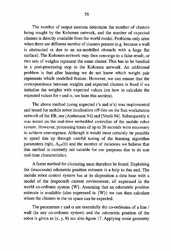
56
The number of output neurons determine the number of clusters
being sought by the Kohonen network, and the number of expectedclusters is directly available from the world model. Problems only arise
when there are different number of clusters present (e.g. because a wall
is obstructed or due to an un-modelled obstacle with a large flat
surface). The Kohonen network may then converge to a false result, or
two sets of weights represent the same cluster. This has to be handled
in a post-processing step to the Kohonen network. An additional
problem is that after learning we do not know which weight pair
represents which modelled feature. However, we can ensure that the
correspondence between weights and expected clusters is fixed if we
initialise the weights with expected values (on how to calculate the
expected values for r and a, see later this section).
The above method (using expected r's and a's) was implementedand tested for mobile robot localisation off-line on the Sun workstation
network of the IfR, see [Andersson 94] and [Vestli 94]. Subsequently it
was tested on the real-time embedded controller of the mobile robot
system. However, processing times of up to 20 seconds were necessary
to achieve convergence. Although it would most certainly be possibleto speed this up through careful tuning of the learning algorithm
parameters (r|(t), Ajj*(t)) and the number of iterations we believe that
this method is currently not suitable for our purposes due to its non
real-time characteristics.
A faster method for clustering must therefore be found. Exploitingthe (inaccurate) odometric position estimate is a help to this end. The
mobile robot control system has at its disposition a data base with a
model of the (expected) current environment, all expressed in the
world co-ordinate system {W}. Assuming that an odometric positionestimate is available (also expressed in {W}) we can then calculate
where the clusters in the ra space can be expected.
The parameters r and a are essentially the co-ordinates of a line /
wall (in any co-ordinate system) and the odometric position of the
robot is given as (x, y, 8) see also figure 17. Applying some geometry
57
{W}x
Figure 17: Calculation ofthe expected ra values in the robot co¬
ordinate system {RJfrom a modelled wall (line)
we find that the expected location *R'(r, a) (in the robot co-ordinate
system {R}), and hence cluster, of a (world) line *w*(r, a) is as in
equation 23 and equation 24,
{R}r = {W}r- cos (_Wa) _sin( J^a)x
(EQ. 23)
{*}a =
Wa-6 (EQ.24)
where [x, y]T and 9 represent the odometrically estimated position and
orientation of {R} in {W}. Due to the inaccuracies of the odometry the
wall will not appear in the ra space exactly at these co-ordinates (if
they were this whole procedure would have no point in any case),
however, if small movements can be assumed between position

58
updates (which can be done if the real time requirement is met) then at
least the wall should lie within some tolerance or, oa. The measured
and calculated p;=(r, a\ can then be assigned to a cluster Cj according
to the formula of equation 25.
Pi*Cj
This rule is then applied to all the measured and calculated
*R*(r, a), for all the expected lines (r, a)j(j=l ... NumberOfVisibleLines) as found in equation 23 and
equation 24, and for each point the corresponding class (line) is
recorded. The possibility of multiple classes is ignored, a point is
assigned to the class against which it is checked (successfully) last. All
the points receiving no classification are ignored for the rest of the
calculations.
After the classification of all *R*(r, a)'s the values for equation 9
and equation 10 can be calculated as the arithmetic averages of those
values that have been assigned to one cluster.
Additionally this method allows:
Automatically relating the measurement to the modelled line,
in contrast to say the Kohonen method where the
correspondence between the clusters found and expected had
to be determined in a post processing step after the clusteringitself.
Increasing robustness in that only "large" clusters are used
for subsequent calculation. The cut-off being determined byhow many points are present in the cluster.
Consider the example scan and environment of figure 18. The
odometrically estimated position for this scan was x - 1.2,y = 1.2 and
6 = 0.101, the two modelled lines have parameters rj= 0.1, a.j=0.0,
r2= 0.1, a2=1.571, a constant set of tolerances aa - or = 0.2 are in
r -o <.r.^r +aj r i j r
ai-°nSaisai + 0„.
(EQ.25)

59
Figure 18: Example ofraw sensor data (points) together with
the modelled environment (continuous lines). Theraw data is displayed in the odometric co-ordinate
system, the lines in the world co-ordinate system.
effect. After preprocessing and least squares line fitting we have the ra-
space of figure 19. Similarly in figure 19 the expected clusters with
±tolerances are displayed.

60
r-alpha space and expected clusters
Alpha [rad]
e 19: ra-space of the sensor data infigure 18 (dots)displayed together with the rectangles within which
the clusters are expected. Additional clusters are
also present, these are due to unmodelledfeaturesin the environment, e.g. the washbasin located
approximately atx-4.1, y-1.0.

61
After the clustering procedure we can set up the following two
equations for the position (x,y) and orientation (for 8 see also
equation 27 and equation 26).
„0.1010-0.0047-0.02399
6 = r (EQ.26)
1.0606
1.0568
1.2000
1.2000
Solving equation 27 and equation 26 gives us a position of x=1.13,
y=l.12,6=0.0240.
In summary this method works by:
Removing data mat is uninteresting for the purpose of
position update.
Fitting lines to neighbouring points generating a
representation of the range data in which geometric structures
can easily be identified.
Using expectancies, finding clusters in this new space
corresponding to the modelled features.
Constructing and solving a small over-determined system of
equations for the position.
Later on, in the experimental section it will be demonstrated that
this method is: accurate, fast and robust.
This method of cluster extraction is based on calculating the
expected locations of the clusters in order to assign the data to then-
respective clusters. The calculation of the expected locations is based
on world model data and the robots odometric position in the world co¬
ordinate system. Therefore, this method will only be able to use, for the
purpose of calculating the robots position, mose structures which have
1.0000 0
•0.0002 1.0000 X
1.0000 0 y.
0 1.0000
(EQ. 27)

62
been modelled. Any un-modelled structure, such as an obstacle, will
generate a cluster, this cluster, however, will not be used in the
subsequent calculations.
Later on it will be seen that in some cases the clusters will not be
as distinct as desired, particularly in the case of a cylinder. This can be
alleviated by introducing a measure of quality to all the points under
considerations, and only to consider those points which have a
minimum quality in the clustering procedure. The exact quality
measure will vary depending on the particular structure "behind" the
cluster, and the quality measures will therefore be defined in the
appropriate sections.
3.5.4 Position from a corner
A corner is in many ways similar to a co-ordinate system, and co¬
ordinate transformations could be used to calculate a mobile robot
position if the transformations between the corner co-ordinate system
and the robot system as well as the transformation between the world
co-ordinate systems and the corner co-ordinate system were known. In
this work this will not be exploited for the following reasons:
The corner is a junction between two walls and the robots
orientation can be extracted directly from walls (see previoussection), using the corner orientation would amount to usingredundant data.
If the orientation of the robot co-ordinate system with respectto the world co-ordinate system is known then the positioncan be calculated by simple geometry. Furthermore, it is safe
to assume that the robots orientation is known since in the
presence of a corner at least two walls are present which yieldthe orientation.
Referring to figure 20 the mobile robot position in the world co¬
ordinate system, ^x and Wy, is given as in equation 28 and

63
equation 29.
{W} {W} I {R} . {R} .A
x= xc-\ jcccos8- ycsm8l (EQ.28)
{w} {w} ( {R} .. {R} _\
y= yc~[ xcsmQ+ ycCOsQ) (EQ.29)
Figure 20: Example ofa corner in the sensor and the world co¬
ordinate systems.
Here ^whc is the x co-ordinate of the comer in the world co-ordinate
system,' w'yc is the y co-ordinate of the comer in the world co-ordinate
system, ^xc is the x co-ordinate of the comer in the robot co-ordinate
system, ^yc is the y co-ordinate of the comer in the robot co-ordinate
system, and 8 is the orientation of the robot co-ordinate system with
respect to the world co-ordinate system.
Using equation 28 and equation 29 it is possible to extract the
position of the robot co-ordinate system directly. Hence, it is easy to
integrate the positional information from comers with that from walls

64
through adding rows to the equation for position (see equation 27). For
each corner it is necessary to add two rows, one corresponding to ''y
and one corresponding to ^wh. An example of such an equation for the
robots position is given in equation 30,
(m',-<%)("V <*>,,)
mxm
{W} . {W}cos cij sin Oj
. {W}a2 sin a2= cos
{w}
1
0
0
1
(EQ. 30)
where the first two rows are contribution from walls and the last two
rows a contribution from a corner. Hence, the task is reduced to the
same as for the straight line, to find corners in the sensor data.
3.5.5 Extracting corners
A number of methods are available for corner extraction in range
data. A discussion of several of the different methods, e.g. template
matching and matched filtering, can be found in [Vestli95]. In this
work, however, it is of advantage to exploit the pre-processing carried
out for the detection of walls (see section 3.5.2) for the purpose of
corner detection. Exploiting the data produced by the processingmentioned in section 3.5.2 has the advantage that the edge detection
can be implemented without the need for large amounts of additional
processing power.
In figure 21 a range-finder scan together with the lines fitted to
points p and q are displayed. The lines were found using equation 18
and equation 20, i.e. the lines are represented with r, the perpendiculardistance to the line from the origin of the co-ordinate system, and a,
the angle between the x axis of the co-ordinate system and the
perpendicular line. If the points p and q are on different sides of the
corner then the crossing point of the lines fitted to p and q respectively

65
°oo o 5|o o o ^JOujou^tyQ
1
® -I °
Figure 21: A real range-finder scan where two "fitted" lines
have been added. The lines have been drawn
manually and are only meant to aid the
understanding of the corner extraction.
can be used to gain information on the location of the comer. The
crossing point of the two lines, and hence die probable location of the
comer is given in equation 31,
cos a sinap P
cos a sin a1 1\
(EQ.31)
where x and y are the sought variables. Comers can then be found by
applying the following procedure:
1 Let si be the ith measurement point in the scan.
2 initialise i = 1.
3 Apply equation 31 to p = s, and q = si+p where j = 1. k, and k
is a constant (for our experiments we have used fc=5).

66
4 Increment i and if i <= n then repeat from 3, n is the number
of range readings in the scan.
By the above described method a cluster of solutions will form at
the location of the corner. This cluster can then be extracted with the
same methods as described for the straight line case and the mobile
robots position can be found by applying equation 28 and equation 29.
An example of a range-finder scan can be found in figure 22,
Range data
31 1 1 1 1
oo
2 -„° °
^o° o
r—t~
°o
a—'
to
« o
oO°° o
0oo° °0
Vo
o
o
- <oo
o°
oo°° o
K.
>' o
o
o
o o
><o o
o
o
o
0
o
o
1
9,1 - f
1 1 1 1
-2-1012
X co-ordinate [m]
Figure 22: Range data with two potential corners, one at (1.5,2.2) and one at (-2.2, 0.5).
and the corresponding clusters indicating the location of the corners is
visualised in figure 23.
In order to minimise the burden on the processor it is advisable to
include checks before applying equation 31 in step 3 above. If ap and
aq have nearly the same value then they are probably lying on the same
straight wall and we may continue directly with the next q without
solving equation 31. For our experiments we have insisted on a

67
Clusters from corners
3i i i
eF
2 -
6
Y
co-ordinate -
I
(A/
i i i
-2-1012
Xco-ordinate [m]
Figure 23: The result ofthe corner extraction process
(clustering) when applied to the range data offigure 22, two clusters corresponding to the two
potential corners werefound.
difference in a's of the order of Jt/2 ± jt/8. In addition to minimisingthe processor load no difficulties with ill conditioned equations will be
experienced if such a check is integrated.
3.5.6 Position from a cylinder
Further natural landmarks that frequently are found in buildings
are pillars with cylindrical and rectangular shapes. The information on
any rectangular such structures can be extracted with the line fittingand corner extraction described above, hence this section will focus on
extracting position information from cylinders only.

68
Assume that one cylinder is visible to the robot's sensor.
Furthermore, assume that the world cartesian information on this
cylinder ({W}xcy) {W}yCy> {W}rcy), where {w}xcy and {w}ycy is the
centre of the cylinder and ^W'rcy is the radius, is given. Finally, if the
same information on the cylinder can be extracted from the robot's
sensor data in the robot's co-ordinate system (' 'x,
then we may constrain the robot's world position (
equation 32 below, see also figure 24.
{R} {R} n
cy> jcy> Lcy)
Xr, *W'yr) as in
Range of solutions
{W}Ycy
t{W}
yr
{W}
/ {R}r _{W}/ icy- *<•
Cylindrical pillar
{R> /wx
{W}„vcy-
{W},
cy
Figure 24: A cylindrical pillar in the robot {R} and world {W} co¬
ordinate systems. If the information on this cylinder is
known in the world system (' -Oc({W}Y fWi {Wtrc ) and can
be found in the sensor data rR^xcy,' 'ycy, rcy)tnen tne
position of the robot (> 'xr iw'yr)is restricted to lying onthe dashed circle.

69
(,%)Mlsl02 = (°V,"\Jmm
r Jcy,)'
2
+
(EQ. 32)
The left hand side of equation 32 corresponds to the square of the
radius of the circle on which {R} is lying (dashed circle in figure 24),
*R*xcy and ^RVCy is to be extracted from the sensor data. The righthand side of equation 32 corresponds to the common formula for a
circle centred on ^W^xcy and *W*ycy (world model information) with
{w*xr and *w*yr being the sought information (robot position). As this
means that the robot position can be anywhere on a circle we cannot
extract the orientational information of the robot (*w^6r) from a circle
directly.
However, if the orientation, 6, of the robot co-ordinate system {R}relative to the world co-ordinate system {W} is known then it is
possible to use equation 33 and equation 34 to determine the positionalcontribution from the corner.
(EQ. 33)
(EQ. 34)
This is analogous to the case of a corner, see also equation 28,
equation 29 and figure 20.
The problem is again the same as for lines and corners: to extract
circles with their associated cartesian information from the noisysensor data. Consider the case of a number of sensor data points
Pl .. pn, in the robot co-ordinate system (pj = *R*Xp *R*yi), lying on a
circle centred at *R*xc, *R*yc with radius *R*rc. Considering only one of
these n measurements, namely pj, it is possible to formulate
{WK = {W}X -({RK cose-{R}y sine)cy \ cy }cy )
wy ={W}y -{{R}x sin8+Wv cose)
•'cy \ cy 'cy )

70
equation 35.
Expanding equation 35 and rearranging the terms gives equation 36,
-(xf+yf) = -2xtxc-2ytyc+{xc2+yc2-rc2) ^-36>
for the sake of brevity the leading {R} superscripts have been dropped.
Equation 36 may be re-written in matrix form as in equation 37.
(*,2+*2)I - [-**<-*<']x +y -rc Jc c
(EQ. 37)
In equation 37 only one measurement (measurement i) has been
considered. In the case where several measurements are used
equation 37 may be expanded to give equation 38, an overdetermined
system of linear equations with three unknowns xc, yc and qc=xc +yc -
-(*l2 + Vi2)-(*22 + v22)
/ 2 2
-\xn +yn
-2xx -2yj 1
-2*2-2?2 l
-2*„-2y„ 14c
(EQ. 38)
Equation 38 may then be solved for xc, yc and qc using linear algebra.
Applying the formula of equation 38 to successive "windows"
into the sensor data (p; .. pi+n, pi+i .. Pj+i+n, P;+2 • ) a cylinder
manifests itself as a cluster of similar solution in the solution space for
xc, yc and rc in a manner similar to the straight line case presentedearlier.

71
Initial experiments on sensor data indicated that some problemscould be expected on the clustering as linear structures sometimes giveresults that appear close to each other. Therefore a measure of the
quality of the fit was introduced, which allows the rejection of
"solutions" which do not achieve a minimum quality, and which do not
arise from a circular structure.
For the calculation of the quality of the fit the inverse to the sum
of the residuals squared from the solution of equation 38 was utilised.
The residuals rj .. rn are given in equation 39 and the quality of the fit
is calculated according to equation 40.
2xx -2vj 1
2jc2 -2y2 1XC
yc
\
n Jn
?c1
-{xx+y\)-(x22 + y22)
:(xn2+yn2)
(EQ. 39)
Qi = \li= 1
-1
(EQ.40)
As an example on this method consider the graphics of figure 25.
Applying successive least squares fitting to this set of range data the
solutions of figure 26 are produced. In order to separate good from bad
fits a line is plotted with a height which is proportional to the quality of
the fit. One significant cluster can be seen and the average x and y of
this cluster is the information sought. The clustering can be carried out
by methods similar to those explained for straight lines and will thus
not be discussed further.

72
Scan with (semi) circle
1
I o-
-2- :
-2-10123World x [m]
Figure 25: Noisy range data scanfrom our laboratories with a
generated cylindrical pillar located at x=2.0, y=0.0.
3.5.7 Summary of structure extraction methods
In section 3.5.1 to section 3.5.6 a detailed analysis on extraction
of positional information from a number of different geometricfeatures were described. Before progressing onto the issue of
combining all this information a quick summary may be appropriate.
In order to achieve a final compact formulation of the problem of
determining the position of the mobile robot a strategy which matches
structures in the sensor data to structures in the world model was
selected.
In order to improve the quality of the subsequent extraction of
geometric structures the sensor data is filtered. The filters discussed
reject first of all data that are out of range, then any other data which
appear "alone" in the sensor data set and thus have no information on

73
Clustering from circle fit
xlO
~3~
4-1
o
4-»
—-H
3
-5
World y [m] -5 -10World x [m]
Figure 26: A scatter plot of the solutions to the least squarescirclefitting described above. For each solution (x, y)a barproportional to the quality ofthefit is plotted. At
(2.0, 0.0) a cluster ofhigh quality solutions can be
observed, this corresponds to the semi-circle in the
range data offigure 25.
the structure of the environment, finally the data set is "thinned" which
gives a uniform quality of the information, independent on the range,
to any structure.
After filtering a number of methods for extracting geometricinformation were presented. Straight lines (walls) are found through a
least squares fitting of straight lines to subsequent sub-sets of the
sensor data and extraction of clusters in the solution space of the
straight lines fitting. A similar method is used for cylindrical objects,
however, a different least squares fitting approach had to be utilised.
Additionally, it was necessary to introduce a measure for the quality of
the fit when extracting circles. In the case of corner extraction the

74
results from the least squares fitting for the walls were further
exploited. The point where pairs of the straight lines fitted in wall
extraction process cross is a potential location of a comer. In the same
manner as in the case of a wall and of a cylinder clusters form where a
comer is present.
3.5.8 Combination of different geometric information
In the previous sections it has been demonstrated how positionalinformation can be extracted from geometric structures such as walls,
comers and cylinders through a process of pre-processing and cluster
extraction. In the case of walls and comers it has also been shown how
the positional information from the different sources can be combined.
Although it has been shown that cylinders can be found in the same
manner as walls and comers the combination of positional information
from a cylinder with that from a wall or a comer is not quite so easy.
The robot's position can be found from walls and comers by
solving a linear system of equations, see equation 30. In the case of a
circle the equation yielding the position is, in general, quadratic. Onlywhen it can be assumed that the orientation of the robot co-ordinate
system is known with respect to the world co-ordinate system does a
cylinder yield positional information which can directly be combined
with positional information from walls and comers through linear
algebra.
In the general case, when positional information from a circle is
available and the orientation of the robot co-ordinate system with
respect to the world co-ordinate system is not know, an iterative
solution is called for. Re-writing the constraint equations for lines,
points (odometry and comers) and cylinders we may formulate the
following equations for the residuals squared equation 41 to
equation 43.
^("V^f-OV?,)2 <EQ-41)

75
S, = ( {w\cosa/+ {w}yrsmarr^ (EQ.42)
5„ represents the squared distance from a point, Sj the squared distance
to a line and Scy the squared distance to a circle. These equations maybe seen as functions of the "true" robot position ^xr and ^yr and all
the remaining parameters are constants extracted from the sensor data
or provided by the world model.
A least squares solution attempts to find the minimum of the total
error, see also equation 44.
Stot = Sodometry + lSl + 2Scy + lSco <HQ.44)
T cy co
The summed terms indicate that each line, cylinder and corner have
their own contribution and the odometry is one separate contribution.
At the least squares solution the partial derivatives of Stot with respect
to'
'xr and'
'yr must be zero and in the vicinity of the solution we
may consider Stot to be of second degree (i.e. parabolic).
This means that the partial derivatives of Stot with respect to ^w^xrand ^w^yr change sign at the solution and that this sign change is the
only sign change in the close proximity. Thus we may use the method
of bisection (see also [Press 86]) to find the root of the partialderivatives of Stot which also yields the least squares solution to
equation 44.
The bisection method works by initially defining two limits, upper
and lower, which span the solution of the function, i.e. the function
returns different signs when evaluated at upper and lower. The function
is then evaluated at the mid-point of upper and lower and the sign of

76
the mid-point is examined. The mid-point is then used to replace the
limit with the identical sign and the procedure repeats with the
calculation of a new mid-point. This iterative process is continued until
the desired accuracy is achieved. In our case that means that the
procedure is as follows in x (y being equivalent):
1 Define ^W^xr.upper and ^Jcr./0MW. and evaluate the partialderivative of Stot at both values.
2 If the difference *xr_upper and *W*xr_[ower is smaller than a
preset minimum then exit from this iterative procedureotherwise continue with 3.
3 Let xr-midr \ xr-upper^ xr-lower>' *"
4 Evaluate the partial derivative of Stot at ^xr_my.5 If sign(dldx St0^}xr.mid)) * sign(dldx Stof"}xr4ower))
then{W} -{W}
.AAr-upper~ Ar-mia
else
xr-lower~ xr-mid-
6 repeat from 2.
With this method it is then possible to integrate all the positionalinformation gained with the previous feature extraction algorithms,consider also the example below.
In figure 27 an environment which contains one modelled and
sensed wall and one modelled and sensed cylinder is visualised. The
odometric position estimate (indicated with a + in the drawing) is [0.9,
0.9]. The cylinder is located at [2.0,1.0] (in {W}) and has been found
at a radius of 1.0 (in {R}). The distance of the line on which the robot
is located (according to the wall and the sensor data from the wall) is
1.0.
The iterative algorithm above was used to find the least squares
solution to this problem with the following initial values:
{W} =0 9+0 2 {w*x i =0 9-0 2 ^K =0 9+0 2
{w}yr.[ower=0.9-0.2. The iterative solutions are plotted in figure 28 (for
the x co-ordinate) and figure 28 (for the y co-ordinate). After 10
iterations the difference between the upper and lower limits are

77
Actual wall Measurement(s).
Constraint equation /from the wall l ,
1_
/ \Odometric \
positionestimate
<fe -
\
{W}
Actual cylinder
Constraint equationfrom the cylinder
Figure 27: Example environment containing one modelled and
sensed wall, one modelled and sensed cylinder. The
cross indicates the odometric position estimate. The two
structures introduce two constraint equationsfor the
mobile robot position (in addition to the odometry).These equations are visualised with the dashed lines.
negligible 0.78 [mm] (in both co-ordinates) and the solution is [0.9809,
0.9871].
3.6 Scanning while moving
The position update algorithms of this chapter have assumed that
all the separate measurements of the range finder scan have been
recorded in the same co-ordinate system, i.e. with the sensor stationary.
In reality it may be desirable to have the robot moving whilst recording
data, hence the above assumption may not hold.

78
Convergence of x estimate
1.1-
1-
u
f0.9-x
0.8-
0.7-
0.6' ' ' ' ' ' '
0 2 4 6 8 10
Iteration step
Figure 28: Trajectory ofthe iterative solution in the x co¬
ordinate. The upper limit is marked with +, the lower
limit with o and the middle value with x.
To enable scanning while moving the following procedure can be
used. Simultaneously to measuring the first range of the scan the
robot's odometric position, p1; is recorded. Further, simultaneously to
measuring the last range of the scan the robot's odometric position, pn,
is also recorded (there are n separate range measurements in the scan).
Furthermore, we will assume that the robot has made a linear
movement in all degrees of freedom between pj and pn. It is then
possible to transform all the measurement points into one co-ordinate
system, for instance the co-ordinate system of the first range
measurement by using the subsequent equation 45.
The transformations of equation 45 are to be understood in the
following way: the i* measurement, ^xt and ^yi expressed in the co-

79
Convergence of y estimate
4 6
Iteration step
8 10
Figure 29: Trajectory ofthe iterative solution in the y co¬
ordinate. The upper limit is marked with +, the lower
limit with o and the middle value with x.
{1}
Oh
x.
yt
i
cos(^—Ue) -sin(^—Ue) i—U*\n-l / \n-l i n-\
sin(^-Se) cos(^-oe) ^-Uy\w-l / \n-\ I n-\
0 0 1
{'}y>
i
(EQ.45)
ordinate system {i}, is transformed into co-ordinate system {1}. The
values ax, dy and dq are the differences between the x, y and 6 values
ofpj and/?„, respectively.
The magnitude of the robot's movement between the first and the
last measurement in a scan is a function of the robots velocity and the
time delay between the first and the last measurement in the scan. If the
maximum velocity is limited and the time delay is small the magnitude

80
of 6x, ay and oq also remains relatively small. Within the context of
mobile robotics where a maximum velocity of 1 m/s is normal and
where laser range finders can be expected to perform a scan in 50 ms
we expect corrections to a measurement point of less than 5 cm. With
faster sensor systems the magnitude of movement will drop even
further. Since 5 cm is of the same order of magnitude as the
inaccuracies in some laser range-finders it might be that the error
introduced by the moving robot is insignificant compared to the other
error sources. Furthermore, it is likely that laser range finders will get
faster, as these sensor systems are still in their infancy, and that the
maximum velocity of mobile robots will remain at around 1 m/s, as the
danger of injury to people increases with the speed. Therefore, even
with the current state of the technology, it is not to be expected that
scanning-while-moving will present any major problem.
The transformation of the measurement data presented in
equation 45 relies on that the error of the odometry is small for small
robot movements. Wilful disturbance of the system, for example by
moving the robot by hand or by oiling the floor so that wheel spin is
caused, is not catered for. The exact nature of all the possible
"exceptions" will not be known until more experience with the robot
operating in a real environment is available. When this additional
experience is available the "exceptions" will have to be analysed and
resolved on a case by case basis.

81
4 Experiments
4.1 Guide to this chapter
The beginning of this chapter contains a number of "static" tests
that verifies the real-time, accuracy and robustness performance of the
methods for position update introduced in this thesis.
Extended runs of the mobile robot in the mobile robot laboratories
of the Institute of Robotics (IfR), Swiss Federal Institute of
Technology Zurich (ETH) are presented.
The data is provided in graphical and tabulated form as
appropriate.
4.2 Testfor real time performance
As previously stated we believe that it is of fundamental
importance that a position update cycle can be executed in real-time.
The requirement for real-time for mobile robots was defined to be less
than one second. The methods presented in this thesis must now be
measured against this requirement.
The first test for real-time performance was carried out in the
laboratories in the Technopark Zurich. All the algorithms were
implemented in Oberon [Reiser 92] and executed on the mobile robot

82
embedded computer, a Motorola 68020 card running at 12 MHz
[Motorola 87], under the real time operating system / developmentenvironment XOberon [Diez 93].
For the purpose of timing the measurements the hardware timer of
the mobile robots embedded computer was used. This timer provides a
resolution of one millisecond.
For the first test the robot was placed so that the sensor data
contains many readings (« 50% of the total number of readings) from
the modelled environment. The odometry and the world map was
initialised to a value "near" to the "true" value. A number of position
update cycles were then performed and their execution time recorded.
Only one parameter was changed during this experiment, namely the
number of raw sensor data.
The results of these tests are shown in figure 30 to figure 32. As
expected, we observe an almost linear dependence on the raw sensor
data. This is expected since the majority of the processing steps are
linearly dependent on this parameter. Furthermore, we observe that
even for large data sets (300 raw data per 2?t) a total processing time of
approximately 0.5 s only is necessary. It should be remembered that in
parallel to the position update algorithms there are a number of high
priority tasks running, such as the steering-angle controller, the
propulsion-velocity controller, the odometry and the laser-scanner
mirror-velocity controller. These all interrupt the position update
algorithm. The time needed to acquire the data is currently 1 second,
but this is not included in the figures. The data acquisition overhead
can easily be reduced, for instance by using the industrial sensors
which have just been introduced, see [Sick] and [Leuze]. In particularthe sensor from Leuze Electronic is capable of transferring 720
separate measurements to the main computer in 200 ms [Argast95].
Through pipelining of the process, i.e. by starting data processingbefore completion of data transmission, the time delay generated bythe data acquisition could be further reduced. However, the time
needed for the data processing algorithms themselves is more than 200

83
Processing time for position update
0.1550 100 150 200 250 300 350
Number of "raw" data in scan
Figure 30: Total cpu time as aJunction of "raw" laser scanner
data. The errorbars indicate the standard deviation
observed.
ms, and therefore any effort in improving the position update methods
presented in this thesis should focus on the data processing and not on
the data transmission.
The above tests for real time performance only use straight lines
and the odometric position estimate for localisation. Hence, the
different processing steps correspond to the functions described in the
previous chapter as listed in table 3.
The next significant factor that influences die processing time
(after me number of raw data points) is the number of modelled
structures. The time required to complete step 9 will increase with

84
Processing time for update
4 6
processing step
10
Figure 31: Percentage accumulated as afunction ofthe positionupdate subroutines.
increasing number of structures. However, it is seen that this time is
only some 25% of the total time and that it is combined with other
book-keeping functions. Additionally, we do not expect to have very
large numbers of modelled structures, as the set of relevant structures
is limited by the rough position (odometry) and the maximum range of
the sensor.
It is expected that significantly faster processing times can be
achieved with a later generation of processor cards (e.g. 68040), and in
a multi processor environment the overhead load of the controllers can
be reduced through distribution over available processors. Thus with
only minor modifications one can expect to be able to achieve
processing times in the order of 200 ms even for large problems.

85
Processing time for update
4 6
processing step
10
Figure 32: Percentage ofthe CPU timefalling on each individual
sub-routine of the position update algorithm.
4.3 Testfor repeatability
In section 3.2 the requirements with respect to the repeatability of
the localisation algorithm were discussed, and a repeatability of ±10
mm was identified as adequate for the purpose of mobile robot
positioning. In this section the methods presented in this thesis are
tested for their repeatability.
The robot was placed in a "dead end" corridor and provided with
an initial position estimate, a number of parameters of the algorithms
and a data base containing the coordinates of the 3 visible walls. The
details of the initialisation values are provided in table 4 to table 6
below.

86
Processing step
number Localisation "sub-routine"
1* Acquisition of data (retrieval
from another module)*
2 Range limitation
3 Conversion from polar to Car¬
tesian representation
(equation 5)
4 Rejection of unsupportedmeasurements
5 Thinning of data set
6* Book-keeping function*
7 Calculation of the two sums of
equation 20
8 Calculation of r and
(equation 20 and equation 18)
9(*) Bookkeeping functions* plus
matching of clusters and solv¬
ing system of equations
(equation 25, equation 26 and
equation 27)
Table 3. Correspondence between graphics and method described
earlier. The processing steps marked with * do not participate in the
update process but are included for technical reasons.
Coordinate Initial value
X 1.02 [m]
y 0.89 [m]
e 0.001 [rad]
Table 4. Initial odometry values
After initialisation repeated cycles of the position update
algorithm were performed, each time with new range data. The x-, y-

87
Identifier r a
Walll 0.1 [m] 1.571 [rad]
Wall 2 0.1 [m] 0.0 [rad]
Wall 3 2.21 [m] 1.571 [rad]
Table 5. Content of the data base for accuracy tests
Parameter name Value
Number of range data evenly distrib¬
uted over 2jt before any filtering.
300
Number of elements in line fitting. 7
Maximum range 4.0 [m]
Minimum range 0.5 [m]
Maximum distance to neighbour point 0.3 [m]
Minimum distance to neighbour point 0.06 [m]
Minimum number of points in cluster,
i.e. a cluster containing less points is
removed from subsequent steps.
1
Size of cluster (a) ±0.2 [rad]
Size of cluster (r) ±0.2 [m]
Table 6. Parameters of the position update algorithms
and 8-values of the robot position were recorded. In figure 33 to
figure 35 the recorded values are visualised. Due to a rather large error
in the initial odometric value only the last 25 measurements are
visualised. Inspecting these figures it becomes clear that the accuracy
is high, a condensed tabulated result is found below in table 7.

88
Sensor supported x position estimate
15 20Measurement number
25
Figure 33: Time history ofthe x position estimate when testingforaccuracy. In this context a measurement refers to the
whole processfrom data acquisition through to solvingfor the robot position.
Coordinate Standard deviation
X 3 [mm]
y 4 [mm]
e 0.3°
Table 7. Accuracy / repeatability of the sensor supported robot
position estimate.
4.4 Testfor robustness
As mentioned in section 3.2.1 it is important to test the
performance of the position update algorithms under less than optimal

89
Sensor supported y position estimate
10 15 20
Measurement number
25
Figure 34: Time history ofthe y position estimate when testingforaccuracy.
conditions. Below an attempt at demonstrating the tolerance of the
method is presented.
The mobile robot was placed in a position where two walls could
be seen, see figure 36. The walls were perpendicular to each other. The
data base was updated with the coordinates of the two walls and the
initial odometric estimate was initialised to an accuracy of a few
centimetres and degrees.
After initialisation a number of position update cycles were
performed. Each update includes the following processes: acquisitionof range data, filtering, matching, least squares solution of over
determined system of equations. The new estimated robot position was
recorded and used to over-write the old estimate. After a number of
such cycles a disturbance was introduced that partially blocked the
view of one of the walls, see figure 37. With this disturbance another

90
Sensor supported phi orentation estimate
5 10 15 20 25
Measurement number
Figure 35: Time history of the orientation estimate when testingfor accuracy.
set of position update cycles were performed. Subsequently, more and
more disturbances were introduced, until the algorithm "failed", see
figure 38 to figure 40. The various program constants for this
experiment are listed in table 8.
For each situation 10 measurements were taken. Below in table 9
an overview of the algorithms "robustness" is given. The methods
employed must be said to be robust. Despite introducing even majordisturbances, partially blocking the sensor's view of the structures, the
variance of subsequent position estimates has the same order of
magnitude as in the ideal case. Nevertheless, a few effects are worth
considering in more detail. In particular it is interesting to note that for
an occlusion of 100% the standard deviation in the y direction is 0.
What happens is that the algorithm fails to find the wall (i.e. cluster in
the ra-space). Therefore no entry is made which provides a correction
in the y-direction. The y estimate therefore remains stable at its last

91
Walll
Origin of {R}
Robot
Wall 2
Door, not modelled
Figure 36: The robot displayed in the "perfect" environmentforrobustness test
value. This is expected in this situation since the walls are parallel to
the world x & y axis. In an environment where this is not the case, or
where more walls are present this effect is not observed.

92
K\\\\\\\\\\\\\\\\\\\\\\\\\\\\\\\\\\\\\\V
Blind zone
Figure 37: 30% of Wall 2 is obstructed by an obstacle
4.5 Positioningfrom corners
In the previous sections only those part of the position updatemethods which use straight walls were tested. In this section the
positioning using corners will be tested.

93
Obstacle
Blind zone
$
S
Figure 38: 60% of Wall 2 is obstructed by an obstacle
However, before progressing, it is important to notice that the
laser range finder utilised in the previous section [Acuity] was replaced
with an industrial sensor [Sick] prior to the experiments of this section.
Furthermore, it is important to notice that the industrial sensor has a
range resolution of 5 cm. This means that the "Sick sensor" compares
unfavourably to the "Acuity sensor" and hence that the results

94
RX\\\\\\\\\\\\\\^^^\\\\\\\\\\^N^^^X]
Obstacle
Blind zone
Figure 39: 80% of Wall 2 is obstructed by an obstacle
presented in this section will be somewhat inferior to those presentedin the previous section. Apart from the replacement of the sensor
system the experimental setup was not changed.
The positioning from corners presented in this thesis utilises the
results from the positioning from walls, such as the r and a values
generated from the least squares fitting and the orientation of the robot

95
Figure 40: The robot displayed in a modified environment; here
100% ofWall 2 is no longer visible
co-ordinate system with respect to the world co-ordinate system.
Therefore only those results which relate directly to the "additional"
processing needed to find the robots position from a corner is
presented.
For the purpose of testing the positioning using corners the same
procedure as in the previous section was followed. The robot was
placed so that a corner was visible and the position estimate initialised

96
Parameter Value
Number of "raw" range data 300
Number of elements in line fitting 7
Maximum range 4.0 [m]
Minimum range 0.5 [m]
Maximum distance to neighbour point 0.3 [m]
Minimum distance to neighbour point 0.06 [m]
Minimum number of points in cluster 1
Size of cluster (a) ±0.2 [rad]
Size of cluster (r) ±0.2 [m]
Table 8. Position update and prefiltering parameters for robustness
test
%-ageobstruction Figure
Std. dev. x-
coordinate
Std. dev. y-
coordinate
Std. dev. 0-
coordinate
0% figure 36 4.7 mm 6.0 mm 0.50°
30% figure 37 3.9 mm 7.6 mm 0.49°
60% figure 38 3.4 mm 7.8 mm 0.81°
80% figure 39 4.1 mm 5.2 mm 0.43°
100% figure 40 3.4 mm 0.0 mm 0.56°
Table 9. Performance of the algorithm
close to the true value. Subsequently a number of position update
cycles were performed and the calculated position as well as the
required CPU time for these calculations were recorded.
The necessary CPU time used for the positioning as a function of
update-cycle number is visualised in figure 41. Thus, positioning from
a corner imposes a time penalty of 100 ms or less. In figure 42 the time
history of the x co-ordinate recorded during the testing is visualised.
The standard deviation is 15 mm which is somewhat more that what
was recorded when considering walls only. This is due to the
unfavourable performance of the "Sick-sensor".

97
100
99
-a v»coou
M 97
& 95
Processing time for corner extraction
94
93.
Mean value: 95.33 ms
Std. dev.: 1.572 ms
5 10
Measurement number
15 20
Figure 41: Processing time for positioning using a corner as a
function of the update cycle number.
4.6 Overall performance
Finally, it is necessary to verify that the algorithms also work
when the mobile robot is moving. This is notoriously difficult to verifysince it needs an absolute reference. Of course such an absolute
measurement system could be made available (see section 2.2.7),
however, these systems are expensive, require significant installation
work and integration efforts into the experimental setup. And in a last
instance, such a system is not available at the IfR, ETHZ.
Rather than comparing the position estimate to an absolute
reference we compare it to the purely odometric estimate, and also
through ensuring that the last position of the trajectory is the same as

98
Corner localisation (x)1.7
1.65-
c
I 1-6
oOh
X
1.55
1.5
Mean value: 1.597 m
Std. dev.: 0.01534 m
0 5 10 15 20
Measurement number
Figure 42: The x co-ordinate as a function of the update cycle.
the start position, i.e. that the robot is expected to move on a closed
trajectory. We expect that the purely odometric position estimate will
have a measurable error at the last position (i.e. the last positionestimate will not correspond to the start value). In contrast to this we
expect that the position estimate gained by using the algorithmsdescribed in this thesis will be close to the true value (i.e. the last
position estimate will correspond to the start value).
The tests were executed in a stop, look, update, move fashion. The
movement commands were provided by an operator, as was the
command to update the position. The maintenance of the world
reference model (i.e. which walls were theoretically visible) was also
taken care of by the operator. A sketch of the test trajectory is shown in
figure 43. Initially the robot was located at A, it was then driven along
a more or less straight trajectory to B where an approximate 90°

99
clockwise negative angle turn was undertaken. From B the robot was
driving in the negative y direction until C, the robot was then reversed
from C until D. At D the robot was turned clockwise on the spot
approximately 180°. Subsequently the robot was reversed back to E
where a 90° turn was again undertaken, and finally the robot was
reversed to near its starting position (and also orientation) A.
Trajectory for "dynamic" testing
3-
2-r—l
J,
T3 I"
o
o-
-1-
-2 b i . . . , , ,
0 2 4 6World x [m]
Figure 43: Test trajectory for the position update algorithms
When executing the above described trajectory the robot
maintained two independent position estimates, one based purely on
odometry and one provided by the algorithms presented in this thesis.
The two separate position estimates are plotted in figure 44. It is
obvious that even for this simple movement it would be fatal to rely
only upon the odometry. The odometry is nearly 1 m off at the end of
the trajectory.

100
Distance sensor supported to odometric estimate
•a 1
o
0-
-1
-2
1-
1 i ]
'/r
/ I
*
~~
\ \
,
- i \-{I1
"True" estimateI1i'
— Odometry
-
0 2 4 6
World x [m]
Figure 44: Sensor supportedposition estimate (continuous line)and purely odometric estimate (dashed line)
4.7 Scanning while moving
In chapter 3 a method for transforming measurement data
recorded with a moving robot so as to appear as being recorded with a
stationary robot was presented. This method has been tested on the
robot equipped with the "Sick-sensor".
The sick sensor completes a 180° scan in 0.05 seconds, this means
that the movement of the robot from the first to the last measurement is
small. In our tests we have been using velocities of up to a maximum
of 1 m/s, which we think is a reasonable maximum velocity, and
therefore the robot moves a maximum of 5 cm between the first and the

101
last measurement. This movement is the same order of magnitude as
the measurement accuracy of the "Sick-sensor", hence it is not possibleto detect any difference between an "uncorrected-scan" and a
"corrected-scan". The same argument applies to the rotation of the
robot, even at rotational velocities of up to 90 7s no difference between
the "uncorrected-scan" and the "corrected-scan" can be observed. This
is in line with the discussions in chapter 3 where the problems of
scanning while moving was seen to be insignificant at a high scanningrate.
4.8 Discussion
The position update methods explained and tested in this thesis
are functional. In fact all the requirements set out at the beginning in
table 2 have been fulfilled. The methods tested in this section exploitinformation from the walls, the corners and the odometry. With respect
to cylinders only a slight increase in processing power consumption, at
the same order of magnitude as the extra processing power required by
positioning using corners, is expected. However, it has not been
possible to test this part of the position update algorithms since no
cylindrical structures are available in our laboratories.

102

103
5 The robot
5.1 Guide to this chapter
In this chapter the electrical and mechanical hardware which was
used to verify the position update algorithms is briefly presented. The
integration of a commercial laser range finder sensor with the
necessary interfacing is described before the capabilities and structure
of the robots control system and control computer is discussed. Under
this last point we will describe how we integrated the position updatealgorithms with the rest of the robot control software.
52 The mobile platform
A three wheeled mobile robot has been constructed at the Institute
of Robotics, Swiss Federal Institute of Technology for the purpose of
serving as a test bed for mobile robotics.
This work was initiated in 1990 with the constructive efforts of
Michel [Michel 91]. In addition to the requirement that the robot
should fit within the MODRO (MODular RObot) concept [Nielsen 92]
some measure of "rough terrain" capability was desired (steps of up to
6 cm should be traversable). Thus a three wheeled mechanism with
large wheels (r=0.185 m) was selected. Additionally, the wheels have
air filled tyres. A three wheel construction ensures that all three wheels

104
always have ground contact and the size and type of wheels makes it
possible to traverse the "terrain". Additionally, to reduce the effects of
any such uneven features all three wheels have independent
suspension. The wheel modules developed by Michel are assembled
onto a frame and all the necessary electronics and computing facilities
integrated. An overall picture of this mobile robot is shown in
figure 45. The critical data for this mobile robot platform is listed in
table 10.
Figure 45: A photo showing the mobile robot experimentalplatform from a "rear and right-hand"perspective.

105
Identifier Value
Width 0.69 [m]
Length 1.10 [m]
Height 0.49 [m]
VME bus size 5 slot (24/16)
Battery capacity 1368 VAh
Steering angle limitations None
Minimal turning radius 0
Area swept at min. turn¬
ing radius
2.43 [m2]
Table 10. Key data mobile robot experimental platform.
The mobile robot has a mechanical configuration as sketched in
figure 46. Equation 46 represents the kinematic differential equations.
(0
r
X
1
w6(0
\{R)m]wm = u>(t)r
Lw«wJ
cos(k(t))
0
sin(X(Q)/
(EQ.46)
= the instantaneous front wheel angular velocity= the front wheel radius
= the steering angle= the axis distance
= instantaneous robot velocities in the robot co¬
ordinate system
We observe that in the y-direction of the robot the velocity is always
zero (under the assumption that the friction is high enough to avoid
slippage). These velocities can be mapped into velocities of the world
co-ordinate system by means of equation 47,

106
Front
Wheel
{W}Rear
Wheels
Figure 46: Kinematics of the mobile robot experimentalplatform.
{whit) "cos(we)o{W}y«)
We(0s,n(we)o
0 1_
x(t)
(t)
(EQ.47)
where ' '6 is the instantaneous rotation angle of the robots co¬
ordinate system {R} with respect to the world co-ordinate system
{W}. The control system sample rate is At=10 ms, which means that
every 10 ms new values for the robot velocities and robot co-ordinates

107
can be calculated. This allows us to express the change in robot
position as in equation 48.
{w,m» mm
wAyW = to mm
mmt) mm
Equation 46 to 48 enable the implementation of a dead reckoning
(see footnote 1. on page 10) position estimation system, throughnumerical integration (summing) of the left hand side of equation 48.
A consequence of the implementation of such a dead reckoning
position estimation system is that * '8 in the transformation matrix of
equation 47 is a function of time.
Any systematic error in the steering angle, X, the wheel radius, r,
or the axis distance, 1, will cause an accumulation of errors in the
estimated position. Therefore position update algorithms based on
environmental sensor data is necessary.
5.3 Scanning laser rangefinder.
As discussed in section 3.3.2 it is necessary to make high quality
range data available to the robot, and in particular the software
components that ensure high accuracy of the instantaneous positionestimate. Therefore such a sensor system was integrated onto the
mobile robot platform. The sensor itself was purchased from the
company Acuity Research [Acuity]. The sensor consists physically of a
cylinder with a diameter of 76.2 mm and a length of 139.7 mm.
Through one end of this cylinder an intensity modulated laser beam is
transmitted and the returning from a target reflected light admitted and
focused. This sensor delivers a 4 - 50 MHz square wave output
representing the ranges 12 - 0 m. Additional analogue outputs indicate
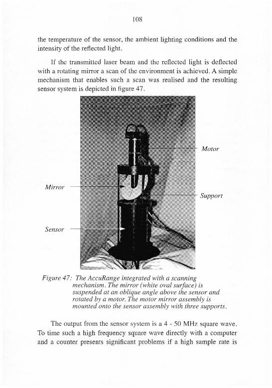
108
the temperature of the sensor, the ambient lighting conditions and the
intensity of the reflected light.
If the transmitted laser beam and the reflected light is deflected
with a rotating mirror a scan of the environment is achieved. A simplemechanism that enables such a scan was realised and the resulting
sensor system is depicted in figure 47.
Mirror
Sensor
Motor
Support
Figure 47: The AccuRange integrated with a scanningmechanism. The mirror (white oval surface) is
suspended at an oblique angle above the sensor and
rotated by a motor. The motor mirror assembly is
mounted onto the sensor assembly with three supports.
The output from the sensor system is a 4 - 50 MHz square wave.
To time such a high frequency square wave directly with a computer
and a counter presents significant problems if a high sample rate is

109
desired. As the rest of the outputs of the laser scanner are available as
analogue signals a high precision frequency to voltage converter was
constructed. The principle of the electronics is sketched in figure 48.
ImpedanceMatching
Pre
amplifier
Divide byn counter
Clock
generator
"
Peak
generatorOne shot Integrator
Low
passfilter
Figure 48: Thefrequency to voltage converter electronics (blockdiagram) that was integrated with the sensor and the
mobile robot platform.
Through the addition of these electronic components and due to
sensor internal operation a non-linear relationship between the output
voltage from the electronics and the measured range exists. It is
necessary to compensate this non-linear relationship. A calibration
procedure must therefore be followed. The sensor system and a well
defined target (Kodak grey card) is mounted onto a relatively stable
aluminium profile. The mirror is adjusted so that the laser beam is
transmitted along the aluminium beam to the centre of the target. The
accurate distance between the centre of the mirror and the target alongthe transmitted laser beam is measured using a tape measure.
Subsequently a number (100 or more) range readings are performedwith this setup and the analogue to digital (AD) converter values
recorded. Plotting the relationship between the actual range and the
mean of the AD converted values (ADvalue) yields the relationship of
figure 49.
In order to convert the ADvalue to the true distance, /, in metres a
polynomial function was fitted according to the least squares principle.

110
Calibrated sensor
2000 3000 4000 5000 6000 7000AD value
Figure 49: The measured ranges andAD converter values
(circles) together with afitted transferfunction.
The function performing the conversion from ADvalue to true distance
is found in equation 49.
/=12
1,85ADvalue
(EQ. 49)
5.4 Robot controller
The mobile robot platform is equipped with an embedded
controller. This controller is based on a 5 slot VME bus [VITA]. The
VME bus contains 2 peripheral interface cards from Mikro Elektronik
Ntirnberg [MEN], the remaining three slots are available for embedded

Ill
computers. Currently there is only one 68020 processor board beingused.
The robot's embedded controller is programmed in the high level
language Oberon with the aid of the development environment
XOberon [Diez 93]. XOberon makes resources such as target specific
compilers, incremental linkers and loaders, embedded file systems and
target debugging facilities available.
Obviously calculation of a mobile robots position is not the only
requirement. Other researchers have summed up the necessary tasks of
mobile robotics to be the ability (for the robot) to answer the following
questions: "where am I", "where am I going" and "how should I get
here". The first question has been answered in this thesis. The latter
two have been addressed in other works carried out at the Institute of
Robotics [Tschichold-Gurman 95] and [Durand 94].
In order to put the process of mobile robot positioning into
perspective it is interesting to consider the whole control structure of
the mobile robot used for the experiments in this thesis. A graphicalview of the overall structure can be seen in figure 50.

•uais&sdivpdnuopisod9i[t01spuods3uuooasdijpp3vpim\ssojLoayx•uuofivjd\mudwuddxa
loqojLd\iqovuav\iaofzunwiutsdinrnfos3t/;/oifztays-'OS^n^!J
ZU

113
6 Conclusions
6.1 Guide to this chapter
For the convenience of the reader we will revise the motivation
for and the requirements of range-sensor based position update
algorithms for mobile robots. A summary of the achievements
discussed in this work will then be provided before a view of what may
come is presented
6.2 Mobile robot positioning, problems and
requirements
A mobile robot may deduce its position and orientation throughnumerical integration of its kinematic differential equations (see
section 5.2), a method of positioning also known as odometry or dead-
reckoning. There are a number of error sources in these equations, such
as: noise in the sensors providing the instantaneous kinematic values,
unknown offsets due to imprecise mechanics and uncertainties due to
complex contact relationships between the wheels and the surface.
These errors are integrated which means that any systematic error,
however small, will over time grow and take on unacceptable values.
An example of such behaviour is demonstrated in one of the
experiments (see figure 44) where at the end of a trajectory length of a

114
few metres the distance between the instantaneous "correct" position
and the position estimated through the odometry is nearly 1 m.
It is thus necessary to frequently update the mobile robots position
using some sort of absolute positioning system. The process of
achieving accurate knowledge of the mobile robots position is the
theme of this thesis. In particular we have focused on achieving
absolute positioning through using optical range finder data, filtering of
this data, extraction of geometric structures in the range data and
matching these to a model of the environment.
6.3 Discussion of thesis
After a general introduction to mobile robotics and navigation in
chapter 1 a thorough literature review was undertaken in chapter 2. The
most common way found in the literature of calculating the robot
position (other than odometry of course) is to exploit geometric
knowledge about the environment. The geometric information exists in
two forms a) as a model (known somehow) and b) in sensor data
extracted from the environment. Matching these two representations
yields the robot position. This process of estimating the mobile robot
position from correlation of environmental sensor data and a world
model has been a theme ever since the early days of mobile robotics.
The investigations of Cox (at AT&T) and WeiB (at the Universityof Kaiserslautern) has been seen as highly relevant to this work as both
consider range data from optical coaxial systems. Cox matches each
separate range reading to entries in the world model and based on this
calculates the robots position. Matching each separate range reading to
an entry in a world model is a rather processing intensive task since a
number of iterations is needed before convergence, and at each
iteration step a new matching process must be undertaken. WeiB on the
other hand uses convolution techniques and matches one scan to the
previous. For the sake of efficiency the convolution is performed on
integers, hence accuracy is lost.
115
Another bulk of work has been undertaken on ultrasonic range
data. MacKenzie uses much the same method as Cox (point to
structure matching), but there are also other approaches such as
Leonard with structure to structure and Crowley with occupancy grids.
Generally ultrasound systems seem to be inferior to optical systems.
We also see that structure to structure matching performs slightly better
than other methods. A particularly thorough work is the one byLeonard where successive scans are processed for regions of constant
depth (RCDs) and the behaviour of the RCDs are used to deduce
information on the structure of the environment.
Despite all these efforts a number of unsolved issues still remain,
namely: achieving (simultaneously) millimetre level accuracy, real
time performance and tolerance towards large inconsistencies between
the model and the sensor data (e.g. as generated by an un-modelled
obstacle). Summarised this means that the requirements listed in
table 11 should be met.
Identifier Requirement
Real time performance < 1 second
Accuracy ± 10 mm
Robustness pass test of section 3.2.1
Table 11. Requirements of position update algorithms.
Chapter 3 then detailed how to achieve these requirements.
Initially, prefiltering is applied to the data. Using simple heuristic
filters we are able to transform the initially noisy range data into a
more appropriate form.
After the prefiltering it is desired that geometric structures are
extracted from the sensor data. Three types of structures, namely walls,
corners and cylinders, have been specifically addressed. For all these
examples we have processed the range data so that the identification of
any such structures is simplified. In particular for walls and cylinderswe have employed an explicit least squares fitting of a model
(geometry of a wall and of a cylinder, respectively) to the data, this
116
avoids costly iterative procedures with unknown bounds. In brief this
process goes as follows:
Set index i=l (first measurement)
Choose measurements i to i+n and fit the circle (x, y) or the
line (r, a) to this data in a least squares sense. Save the results
from the fit for later analysis (clustering)
Add 1 to i and repeat until all measurement points have been
processed.
In the space of fit parameters (x, y) or (r, a) identify clusters
of solutions. A cluster appears where such structures (wallsand cylinders) are present.
Corners on the other hand were found by extracting clusters of
crossing points generated by solving a number of simultaneous linear
equations for pairs of the lines extracted when finding walls. In this
way clusters are generated for the x and y position of the corner
analogous to the straight line and cylindrical case.
After the extraction of the parameters for the lines, cylinders and
the corners these are matched to a model. The process of matching is
achieved through using the odometry values as expectation and
assigning measurements/clusters to model values according to the
nearest expectation (from model and odometry).
After this matching it is relatively easy to construct an over-
determined set of equations that can be solved for the "true" robot
position. When only walls and corners are considered the solution can
be found using linear algebra methods. A cylinder, however, makes the
problem non linear, and therefore, is solved with an iterative method
which finds the solution where the partial derivatives of the sum of the
residuals squared is zero. This iterative solution is therefore efficient,
and using the bisection method the relationship between accuracy and
number of iterations is known and independent of the problem.
In chapter 4 all these methods were put to test, and in particular it
was of interest whether these methods comply with the requirements
defined (see table 11). It was not possible to test the cylindrical case for

117
the lack of an appropriate environment and in the case of corner
extraction the noise level was observed to be higher than what was
required. The high noise level was attributed to the particular sensor
system used when extracting corners. The rest of the tests, however,
showed that the algorithms performed as desired, the noise level when
using walls was of the order of 3 mm, the CPU time required was less
than 1 second, and the method proved robust to disturbances. At the
end in chapter 5 a presentation of the robot platform and the sensor
system used for the testing in chapter 4 was presented.
6.4 Contributions
6.4.1 Prefiltering
In this thesis it has been demonstrated that the quality of the
sensor data used for updating the mobile robot position can be
improved by simple heuristic filtering in the spatial domain.
In particular it was possible to gain a uniform distribution of the
sensor data independent of the geometry of the environment. Uniform
distribution is advantageous as it makes any geometric feature positionand orientation invariant with respect to distance from the sensor and
orientation relative to the sensor (within some limits, such as
visibility).
Furthermore spurious sensor data can be rejected. This improvesthe quality of any subsequent feature extraction and removes the
possibility that a "freak" measurement will create subsequent matching
problems.
6.4.2 Abstraction level
A method of structure (such as wall, cylinder or corner) matchinghas been employed, i.e. the association is between extracted structures
in the sensor data and modelled structures in the world model.
Structure to structure matching ensures a very compact simultaneous
118
equation formulation for the mobile robot position. Such compact
equations enables a computationally efficient position update process.
6.4.3 Transformation of sensor data
One sensor measurement alone provides no information on
geometric structure. In order to find structures in a set of sensor data
we have resorted to transformations.
In the case of walls and cylinders the transformation consists of
fitting a model (a straight line and a cylinder respectively) to sub-sets
of the sensor data. The sub sets are so selected that the fit is over-
determined, furthermore, an overdetermined fit ensures some
additional noise reduction. The sub sets are generated by sliding a
window over the original data set (after prefiltering). The output of the
transformations are the fitted parameters, x and y for the circle and r
and a for the line. A positive feature of both these transformations are
that they can be explicitly formulated and hence require limited
processing power. Because of the explicit formulation of the problemreal-time performance was achieved.
In the case of the corner the transformation is implemented by
solving a number of simultaneous linear equations for pairs of the lines
extracted when finding walls. The equations generated from pairs of
lines are easy to solve, hence requiring little additional CPU time.
Furthermore clusters are generated for the x and y position of the
corner analogous to the clusters generated in straight line and cylinderextraction process.
6.4.4 Extraction of features
Extraction of features by finding clusters in these new
representations is efficient. In order to optimize the extraction of
structures the inaccurate odometry was exploited. Especially the
clustering could in this way be implemented in real-time (sub-second).

119
6.4.5 Equation for position
The extracted significant geometric structures from the sensor
data are matched to the model. Matching structures in the sensor data
to structures in the model produces a compact formulation for the
"correct" position since the number of matched features is relativelylow. Consequently it is easy to solve for the position. Matchingstructures in the sensor data to structures in the model also removes
any need for iteration concerning the sensor data. In the case of non¬
linear constraint equation the solution may have to progress in an
iterative way. However, since no new matching must be calculated at
each step, the iterative solution in the case of non-linear constraint
equation is not computationally expensive.
6.4.6 Performance and performance measure
The execution of these position update algorithms has been
demonstrated on a Motorola 68020 processor system running at 12
MHz. Although this is a processor card of inferior performance to what
can be bought today1 the performance is respectable at 0.5 seconds,
considering that the accuracy of the method is very high. Furthermore
the methods demonstrate a certain robustness in that obstacles
blocking the view do not cause the algorithms to fail until taken to
extremes.
Further a method for measuring the performance of the algorithmhas been introduced. Until now the only reference for position updatemethods as discussed in this thesis has been artificial landmark based
systems. Such systems are expensive and therefore we propose to test
the system against itself. The level of noise on successive positionestimates from the same position is an indication of the performance of
the complete position update mechanism (sensor + algorithms). The
measurement of the system performance has also been extended to the
1. Motorola, the supplier of the processor system used by our robot system, hassince come with 2 new generations of the same CPU series and also a new RISC
processor.

120
robustness of the system where un-modelled obstacles are introduced
in an attempt to disturb the position update process. If the process
rejects such disturbances it can be said to be robust.
6.4.7 Summary
In table 12 a summary of the performance of the position update
Process step Repeatability CPU time
Preprocessing Not applicable 220 ms
Wall extraction - 4 mm, 0.3 deg 165 ms
Corner extraction »50 mm 100 ms
Calculating the position Same as for wall and
corner extraction
165 ms
Table 12. Summary of position update algorithms performance
algorithms presented in this thesis is provided. Since the cylinderextraction has not been tested in a real environment no performancedata relating to positioning using cylinders are provided.
6.5 Outlook
Although one may be satisfied with the performance of these
methods there is plenty of scope for improvement. Hoping that some of
the suggestions below will be of inspiration some explanation is
provided.
6.5.1 Reducing processing time.
Although the methods discussed in this thesis execute in
approximately 0.5 seconds for a raw data set of 300 measurements we
believe that it is both possible and desirable to try to reduce this time. A
reduction in the processing time would make the methods applicable to
faster mobile robot vehicles and/or would make the method more
independent of the odometric estimate.
121
An obvious way of reducing the processing time is to apply faster
conventional processing hardware. In this category we count the latest
generation of CISC processors or the new RISC processors. Should
this not be sufficient then one has to consider ways of parallelizing the
problem. A few suggestions are provided below.
Currently the sensor data is processed sequentially and as one
batch, i.e. all raw data are copied from a buffer (filled by the laser
scanner independently of the position update algorithm) then the
following steps are applied to the data set in sequence: 1) check range,
2) convert to cartesian representation 3) check for maximum distance
to neighbour, 4) check for density, 5) transform data (least squares
fitting or similar), 6) find clusters, 7) construct and solve equation for
position.
It should, however, be possible to pipeline this process. New data
points arrive at regular intervals. Each new data point can be checked
for range by one processor and, if within limits, passed onto another
processor immediately. When this second processor converts the
measurement to cartesian the first processor may already start checkingthe next data point. Schematically this process is visualised in
figure 51. As a suggestion it would be possible to let process 1 throughto 4 (indicated by Px in figure 51) run in parallel on different
processors. Each one can perform its sub-task as soon as a data pointarrived on the input data flow (flows 1 to 4). In P5 a small number of
data points are buffered, for instance 4 which would be enough for a
least squares fit for a line. As soon the points of P5 have been buffered
they are all, as one flow, transferred to the fitting process. The arrival of
a new point on flow 5 causes P5 to remove the oldest point from the
buffer and to add the newly arrived one. This new set of data is as
previously passed on to P6. On the arrival of a new data set on flow 6 a
least squares fitting is performed and the data sent out. The buffer in P7
collects the results and passes them on to the clustering when
appropriate. One could imagine parallel execution of several P6s, P7s
and P8s, one for each feature being sought. At the end the results are
collected and a solution for the position is found.

122
Flow: 1
Range CheckPI
Flow: 2
Polar to CartesianP2
'
Flow: 3
Within max. dist.?P3
1
Flow: 4
Within min. dist.?P4
'
Flow: 5
Bufferp<>
Flow: 6
Least SquaresP6
Flow: 7
BufferP7
Flow: 8
ClusteringP8
Flow: 9
Figure 51-.Example pipelining schemefor parts ofthe position update algorithms
6.5.2 Increasing accuracy
Although the current noise level is in the mm and sub degree
range it may be possible to reduce this even further. The most obvious
action is to use a better sensor system than the "Acuity sensor" or the
"Sick sensor". The recent sensor system from Leuze Electronic should
be superior to the two other sensor systems, however, due to time
constraint it has not been possible to test the methods presented in this
thesis with the "Leuze sensor".

123
Currently all the measurements which fall within a cluster are
treated as equally good. However, some least square fits are probablybetter than others. The quality of the fit should be calculated (for
instance 1 divided by the sum of the residuals) and this quality measure
should be used in calculating a weighted arithmetic middle for the
clusters.
This process should also be extended to the least squares solution
of the constraint equation. Each source of constraint (wall, cylinder,..)should be associated a quality measure similar to the above and this
quality measure should be used when solving the equation.
Before the structure extraction takes place the data is subject to
some prefiltering. Currently the prefiltering uses filter parameters that
have been manually estimated. An interesting extension would be
some automatic parameter estimation process that selects the
parameters so as to minimise the subsequent noise in the positionestimate. At the time of writing such investigations are taking place at
the IfR, ETH, using genetic algorithms and neural networks. However,
it is too early to speculate on the potential of these methods.
6.5.3 Extension of the method
Currently only walls, cylinders and corners are considered.
Although this may be sufficient for a large class of buildings it may be
of use to be able to handle different objects (ellipses, spheres). For any
object where a model can be defined the mechanism described in this
thesis would apply, i.e. fit model to successive windows into the data
and extract clusters in the parameter space. However, with increasing
complexity of the model the fitting process also becomes more
complex.
The same applies to an extension into three dimensions. The
complexity would again increase, furthermore we may have to arrange
the range sensor data in a different way as the sense of neighbourhoodnow is 2 dimensional. It might therefore be that structured light

124
systems or indeed CCD camera based systems are more appropriate in
the 3D world.
6.5.4 Odometry calibration
In the experiments we saw that the odometry was very unreliable.
We suspect that this unreliability is caused by errors in the vehicle
kinematics parameters / axis distance, r wheel radius, and A steering
angle offset. It would be useful if these parameters could be estimated
based on the position update methods. If the robot performs a
reasonably complex trajectory and simultaneously records all internal
sensor values (encoder values) as well as position update values it
should be possible to correct /, r and A. An iterative process similar to
the process used in section 3.5.8 is envisaged in order to select the
"true" parameter set for /, r and A, i.e. the parameter set which
minimises the error between the "true" position and the odometric
position. Furthermore, in order to calculate the odometric position for a
given set of /, r and A the whole trajectory must be re-executed. This
re-execution can be done without moving the robot by using the
recorded encoder values.
6.5.5 Speculative clustering & map-building
In the parameter space of the least square fitting or template
matching the structure of the environment can be found. Currently only
those structures are found which are expected. Since the clustering/
optimum extraction process relies on the world model to achieve the
necessary performance only those structures which are modelled can
be found. If a method could be found that in real-time could cluster the
data without relying on any a priori world model it would be possible
to reverse the process and a world model could be constructed. For this
it is necessary to start an investigation into clustering algorithms.
6.5.6 Fusion with ultrasonic data
A difficulty in this work was to efficiently extract corners. It has
been noted in other works that ultrasound sensors at corners deliver a

125
range of constant depth (RCD, see Leonard). The RCDs can easily be
extracted. However, as walls and cylinders also generate RCDs it is not
immediately known which type of geometric structure causes a
particular RCD. It would be interesting to see if the knowledge from
the laser scanner system on the location of walls and cylinders could be
used to label the RCDs from an ultrasonic scan. If so, then the
remaining un-labelled RCDs are caused by corners. This information
can then be made available to the position update system.
6.6 Summary
New methods for position update have been developed and tested.
These methods use the structure abstraction level both for the sensor
representation and in the world model, furthermore these methods
match structures in the sensor data to structures in the world model.
Using structure to structure matching yields a very compact
formulation of the robot position. The calculation of the robot position
is done with tools from linear algebra or, in the case when cylinders are
present, with an iterative algorithm. The transformation from the raw
sensor data representation to the structure abstraction level is
implemented with an initial prefiltering which rejects erroneous data or
data with low information content. In a second stage least squares
fitting and clustering is performed for walls and cylinders. Similarly
for corners, a cluster extraction method on an abstraction of the sensor
data was utilised.
These methods are extendible, as long as a model can be fitted.
The fitting plus clustering technique can be used to extract geometric
information. This geometric information can be included in the
constraint equation for the robot position which is then solved either
explicitly or iteratively in a limited number of steps. The same applies
to template matching and matched filtering.
With respect to the design requirements our methods have met all
the goals set.

126

127
References
[Acuity] N. N., "Commercial Information", Acuity Research
Incorporated, 20863 Stevens Creek Blvd. Suite 200,
Cupertino, CA 95014, USA, 1994.
[Adams 92] Adams M. D., "Optical range data analysis for stable
target pursuit in mobile robotics", doctoral thesis, Oxford
University, UK, 1992.
[Andersson 94] Andersson H., "Verarbeitung der Daten von
Abstandsensoren", Semesterarbeit (Internal report),Institute of Robotics, ETH Zurich, 8 July 1994.
[Argast 95] Argast M., "Personal communications", Leuze electronic
GmbH + Co., Postfach 11 11, 73277 Owen/Teck,
Germany, 1995.
[Badreddin 95] Badreddin E., "Personal communications", Department of
Automatic Control, ETH Zurich, 1995.
[Bernasconi 92] Bernasconi J., "Informationsverarbeitung in neuronalen
netzwerken", lecture notes, ETH Zurich, Summer Term,1992.
[Brownlow 93] Brownlow M. J., "A time-of-flight optical range sensor for
mobile robot navigation", doctoral thesis, Department of
Engineering Science, Oxford University, UK, 1993.
[Courtney 94] Courtney J. D., Jain A. K., "Mobile robot localisation via
classification of multisensor maps", IEEE Conference on
Robotics and Automation, San Diego, USA, May 1994.

128
[Cox 90] Cox I. J., "Blanche: position estimation for an autonomous
robot vehicle", Proceeding of the IEEE/RSJ International
workshop on intelligent robots and systems (IROS 89),
September 4-6, Tsukuba, Japan, 1989, pp 432-439. Also
in: Autonomous robot vehicles, Cox I. J. and Wilfong G.
T. editors, Springer-Verlag 1990.
[D'Apuzzo95] D'Apuzzo N., "Optimisation of LIDAR Data
Preprocessing", Semesterarbeit (Internal report), Institute
of Robotics, ETH Zurich, February 23,1995.
[Diez93] Diez D., Schweitzer G., "Realtime systems for
mechatronics", Second conference on Mechatronics and
Robotics, Duisburg / Moers, Germany, 1993.
[Dubes 93] Dubes R. C, "Cluster analysis and related issues" in
Handbook of Pattern recognition and computer vision,
Chen C. H., Pau L. F., Wang P. S. P. (editors), World
scientific publishing company, pp 3-32,1993.
[Durand94] Durand N., "Globalen planer filr mobile Roboter",
Semesterarbeit (Internal report), Institute of Robotics,
ETH Zurich, July 1994.
[Elfes 87] Elfes A., "Sonar-based real-world mapping and
navigation", IEEE Journal of robotics and automation, Vol
RA-3,No3,Junel987.
[ESP] N. N., "ORS-1 optical ranging system", Sales information
from: ESP Technologies, Inc., 21 Le Pare Drive,
Lawrenceville, NJ 08648, USA.
[Fogle 93] Fogle R. F., "Robots and teleoperators in radioactive
applications", in Robotics and remote systems for
hazardous environments, Prentice Hall, pp 115-133,1993.
[Fukuda93] Fukuda T., et al., "Navigation System based on CeilingLandmark Recognition for Autonomous Mobile Robot",
Proceedings of the IECON'93, Lahaina, Hawaii, USA,
November 15-18,1993
[Hinkel 89] Hinkel R., "Konzeption eines echtzeitfahigen autonomen,
mobilen Systems", doctoral thesis, University of
Kaiserslautern, Germany, 1989.
[Holenstein 92] Holenstein A. A. "Aufdatieren der Position und der
Orientierung eines mobilen Roboters", doctoral thesis,
ETH Zurich, 1992.

129
[Hyyppaa 93] Hyyppaa K., "On a laser anglemeter for mobile robot
navigation", doctoral thesis, Division of Industrial
Electronics, Lulea University of Technology, 1993.
[Jashmidi 93] Jamshidi M., Eicker P. J., editors, "Robotics and remote
systems for hazardous environments", Prentice Hall, 1993
[Jutander94] Jutander J., "Personal Communications", NDC AB, Box
55,43040 SARO, Sweden, 1994.
[Kajitani 91 ] Kajitani M., et al., "Self-locating measurement system for
mobile robot working in the building site", Journal of
Robotics and Mechatronics, Vol. 3, No. 6,1991.
[Kanayama 89] Kanayama Y., "Spatial learning by an autonomous mobile
robot with ultrasonic sensors", Technical Report of the
University of California at Santa Barbara, Department of
Computer Science, TRCS89-06, February 1989.
[Knieriemen91] Knieriemen T., "Autonome mobile Roboter,
sensordateninterpretation und Weltmodellierung zur
Navigation in unbekannter Umgebung", Band 80, Reihe
Informatik, Bohling K. H.,Kulisch U., Maurer H.
(editors), Wissenschaftsverlag, Mannheim/Wien/Zurich,
1991.
[Kohonen 93] Kohonen T., "Selforganising and associative memory",3rd edition, Springer, 1993.
[Kuc 87] Kuc R., Siegel M. W., "Physically based simulation model
for acoustic sensor robot navigation", IEEE transactions
on pattern analysis and machine intelligence, Vol. PAMI-
9, No. 6, pp 766-778,1987.
[Kuipers 87] Kuipers B. J., Byun Y. T., "A qualitative approach to robot
exploration and map-learning", Spatial reasoning and
multi-sensor fusion, Proceedings of the 1987 Workshop,October 5-7, St. Charles, Illinois, USA, MorganKaufmann, 1987.
[Leonard 92] Leonard J. J., Durrant-Whyte H. R, "Directed sonar
sensing for mobile robot navigation", Kluwer academic
publishers, 1992.
[Leuze] N. N., "Leuze rotoScan RS 2/RS 3, die optischenDistanzsensoren", Leuze electronic GmbH + Co.,
Postfach 11 11,73277 Owen/Teck, Germany.

130
[MacKenzie 94a] MacKenzie P., Dudek G., "Precise positioning usingmodel-based maps", IEEE Conference on Robotics and
Automation, May 8-13, San Diego, USA, 1994, pp 1615-
1621.
[MacKenzie 94b] MacKenzie P., Dudek G., "Personal communications",
Centre for Intelligent Machines, McGill University, 3480
University St., Montreal, Quebec, Canada H3A 2A7,
September 1.1994.
[Maddox 94a] Maddox J., "Smart navigational sensors for automatic
guided vehicles", Sensors, Vol. 11, No. 4, April 1994.
[Maddox 94b] Maddox J., "Personal Communications", IntelligentSolutions Inc., One Endicitt Avenue, Marblehead, MA
01945, USA, 1994.
[Mataric 90] Mataric M. J., "A distributed model for mobile robot
environment-learning and navigation", Technical Report1228, MIT Artificial Intelligence Laboratory, May 1990.
[MEN] N. N., "M-Modul-Spezifikation Revision 2.2", Micro
Electronic Niirnberg GmbH, Wiesentalstrasse 40, 8500
Niirnberg 90, Germany.
[Michel 91] Michel T., "Mobiler Modularer Roboter", Semesterarbeit
(Internal report), Institute of Robotics, ETH Zurich, July1991.
[Miller 87] Miller G. L., Wagner E. R., "An optical rangefinder for
autonomous robot cart navigation", Proceedings SPIE
Mobile Robot II, Vol 852, pp 132-144,1987.
[Moravec 80] Moravec H. P., "Obstacle avoidance and navigation in the
real world by a seeing robot rover", doctoral thesis,
Stanford University, CA, USA, 1980.
[Moravec 85] Moravec H. P., Elfes A., "High resolution maps from a
wide angle sonar", IEEE Conference on robotics and
automation, St. Louis, USA 1985.
[Motorola 87] N. N., "MVME133 Data sheets", Motorola Computer
Group, 2900 S. Diablo Way, Tempe, AZ 85282-9602,
USA, 1987.
[NDC 93] N. N., "System Overwiew", NDC Document No. D4-
31017-20 B, NDC AB, Box 55, 43040 SARO, Sweden,
1993.

131
[Nielsen 92] Nielsen E., Hiippi R., "MODRO: A modular concept for
an application adapted robotics system", Proceedings of
the 23rd international symposium on industrial robots,
Barcelona, Spain, pp 495-500, October 6-9,1992.
[Polaroid a] N. N., "Ultrasonic ranging system", Polariod corporation,Ultrasonic components group, 119 Windsor street,
Cambridge, Massachusets 02139, USA.
[Polaroid b] N. N., "Polaroid ultrasonic ranging system handbook
application notes/technical papers", Polariod corporation,Ultrasonic components group, 119 Windsor street,
Cambridge, Massachusets 02139, USA.
[Press 86] Press et al., "Numerical Recepies, The Art of Scientific
Computing", Cambridge University Press, UK, 1986.
[Reiser 92] Reiser M., "The Oberon system. Users guide and
programmers manual", Addison Wesley, 1992.
[Ritter91] Ritter H., Martinez T., Schulten K., "Neuronale Netze",2nd edition, Addison-Wesley publishing company, 1991.
[Romi 94] Romi C, "Personal Communications", Augenklinik,Universitatsspital Zurich, Frauenklinikstrasse 24, 8091
Zurich, 1994.
[RuB93] RuB A., Lanser S., Munkelt O., Rozmann M.,
"Kontinuierliche Lokalisation mit Video- und
Radarsensorik unter Nutzung eines geomterisch-topologischen Umgebungsmodells", 9. FachgesprachAutonome Mobile Systeme (AMS 93), MUnchen,
Germany, October 28-29, pp 313-327,1993.
[Schiele94] Schiele B., Crowley J. L., "A comparison of positionestimation techniques using occupancy grids", IEEE
Conference on Robotics and Automation, May 8-13, San
Diego, USA, pp 1628-1634,1994.
[Sick] N. N. "Tastender Laser-Scanner PLS",
Produktinformation Erwin Sick GmbH, Optik-Elektronik,Postfach 310,79177 Waldkirch, Germany.
[SNT] N. N., "Sonarange Ultraschall-Abstandssensoren", SNT
Sensortechnik AG, Bahnhofstrasse 25, Postfach, 8153
Rumlang, Switzerland.

132
[Solomon 91] Solomon, R. S. Ill, "A mobile robot sonar system", M. Sc.
thesis, Computer Science Department, Naval PostgraduateSchool, Monterey 93943, CA, USA, 1991.
[Simpson 89] Simpson J. A., Weiner E. S. C. (editors), "The Oxford
English Dictionary", 2nd edition, Clarendon Press, Oxford,1989.
[Tschichold-Gurman 95] Tschichold-Gurman N., "RuleNet - A
knowledge-based Neural Network Model with
Application Examples in Mobile Robotics", doctoral
thesis, ETH Zurich, 1995.
N. N., "The VMEbus specification", VMEbus
international trade assiciation (VITA), P. O. Box 192,
5300 AD Zaltbommel, Netherlands.
Vestli S. J., "The development and testing of mobile robot
obstacle avoidance methods", M. Sc. Thesis, University of
Salford.UK, 1991.
Vestli S. J., Tschichold-Gurman N., Andersson H.,
"Learning control and localisation of mobile robots", 10.
Fachgesprach iiber Autonome Mobile Systeme (AMS'94),
Stuttgart, Germany, October 13-14,1994.
Vestli S. J. "Methods of edge detection in range data",Internal report, Institute of Robotics, ETH Zurich, July1995.
von Flue D., "'Localisation' und 'map building' fur
mobile Roboter", diploma thesis, Institute of Robotics,
ETH Zurich, February 15,1994.
WeiB G., Wetzel C, von Puttkamer E., "Keeping track of
position and orientation of moving indoor systems bycorrelation of range-finder scans", Proceeding of the
IEEE/RSJ/GI International conference on intelligentrobots and systems (IROS 94), September 12-16,
Munchen, Germany, 1994.
[VITA]
[Vestli 91]
[Vestli 94]
[Vestli 95]
[von Flue 94]
[WeiB 94]

Curriculum Vitae
Born 30 June 1964,1 grew up in Kirkenaer, Norway and graduatedfrom Asnes videregaende skole with an exam in general and natural
science in 1983. After one year of military service I entered the
University of Salford, England, from which I graduated in 1987 with a
B.Sc. Upper Second Class in Electronic Computer systems. Thereafter
I worked for one year for Simrad Marine, Bergen, Norway, and
Norwegian defence technology, Guided missile division, Kongsberg,Norway. Upon completion of my contract at Simrad Marine I went
back to the University of Salford where I completed a M.Sc. byresearch, with the theme: Obstacle avoidance using artificial neural
networks for a mobile robot. In parallel with my M.Sc. studies in
Salford I worked at Advanced Robotics Research Ltd. on the
development of control software for robot manipulators. Since 1991 I
have been at the Institute of Robotics under the supervision of
Professor Dr. G. Schweitzer.