riley,hobson,bence: mathematical methods - · pdf filetensors! [these notes taken from...

Tensors

[These notes taken from Riley,Hobson,Bence: Mathematical Methods because their treatment is superb with omissions, additions. expansions and digressions]

The quantitative description of physical processes cannot depend on the coordinate system in which they are represented. On the other hand, physical results are independent of the choice of coordinate system. What does this imply about the nature of the quantities involved in the description of physical processes?

(1) Notation

Einstein Summation Convention --> repeated indices are summed over

Examples:

aixi = ajx jj∑ = a1x1 + a2x2 + a3x3 + .....

aijbjk = aijbjkj∑ = ai1b1k + ai2b2k + ai3b3k + .....

∂vi∂xi

=∂vj∂x jj

∑ =∂v1∂x1

+∂v2∂x2

+∂v3∂x3

+ ......

∂ 2φ∂xi∂xi

=∂ 2φ

∂x j∂x jj∑ =

∂ 2φ∂x1∂x1

+∂ 2φ

∂x2∂x2+

∂ 2φ∂x3∂x3

+ ......

Subscripts that are summed over are called dummy subscripts and others are called free subscripts.

Defining the Kronecker Delta

δ ij =

1 if i = j 0 otherwise

⎧⎨⎩

we then have

aijδ jk = aijδkj = aikbjδ jk = bkaijbjkδki = aijbji = akjbjk

(2) Change of Basis

A vector

A with components (A1,A2 ,A3) is written as

A = Aiei

with respect to the basis vectors e1, e2 , e3. We introduce a new

basis e '1, e '2 , e '3 related to the old basis by the relations

e ' j = Sijei

The coefficient Sij is the ith component of the vector e ' j with

respect to the original basis. We then have

A = A 'i e 'i

or

A = A 'i e 'i = A 'i S jiej = AjejAj = SjiA 'i(S−1)ij S jiA 'i = (S

−1)ij Aj

(S−1S)ii A 'i = (I )ii A 'i = (S−1)ij Aj

A 'i = (S−1)ij Aj

where we have denoted the matrix with elements Sij by S.

In the special case where the transformation is a rotation of the coordinate axes(as we saw earlier), the transformation matrix S is orthogonal and we have

A 'i = (ST )ij Aj = SjiAj

Scalars, for example, the scalar or "dot" product of two vectors

A ⋅B (just a number), behave differently under transformations

since they remain unchanged under any coordinate transformation. The behavior of linear operators is also different. If a linear

operator A is represented by some matrix A in a given coordinate system, then in a new (primed) coordinate system it is represented by the new matrix

A ' = S−1AS

We will now develop a formalism to describe all of these different types of objects and their transformation properties. The generic name tensor will be introduced and scalars, vectors and linear operators will become tensors of zeroth, first and second order (the order or rank corresponding to the number of

subscripts needed to specify a particular element of the tensor).

(3) Cartesian Tensors

We first confine our attention to rotations of Cartesian coordinate systems. We assume that the origin remains fixed and we define the transformation in terms of the components of the

position vector in the old e1, e2 , e3( ) and new e '1, e '2 , e '3( ) bases. We have

x 'i = Lij x j

In this case the transformation matrix L is orthogonal so that

L−1 = LT

or

L−1L = LT L = LLT

LikLjk = δ ij = LkiLkjThis allows us to write

xi = Ljix ' jsince

x = x jej = x ' j e ' jx ' j e ' j ⋅ e 'i = x je 'i ⋅ ejx ' j δ ji = (e 'i ⋅ ej )x jx 'i = (e 'i ⋅ ej )x j

We then have the result

Lij = e 'i ⋅ ejWe note that the product of two rotations is also a rotation. For example, suppose

x 'i = Lij x j and x ''i = Mijx ' jx ''i = MijLjk xk = (ML)ik xk

which implies that ML is also a rotation.

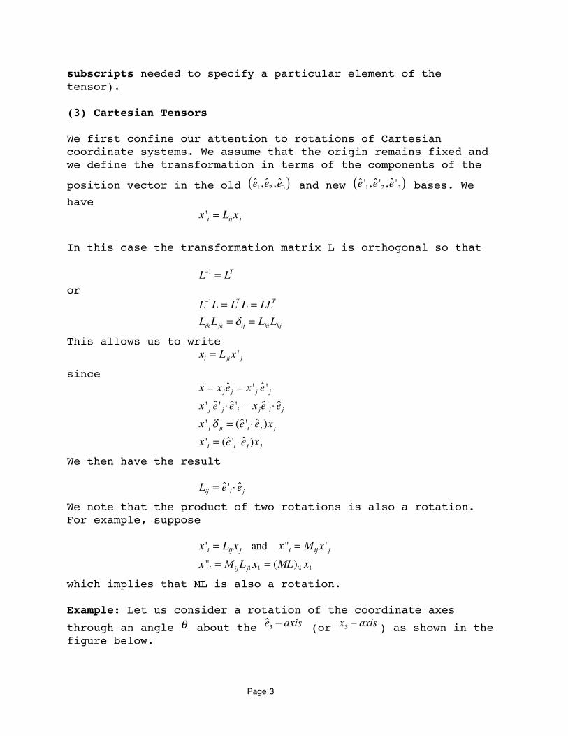
Example: Let us consider a rotation of the coordinate axes

through an angle θ about the e3 − axis (or x3 − axis ) as shown in the figure below.

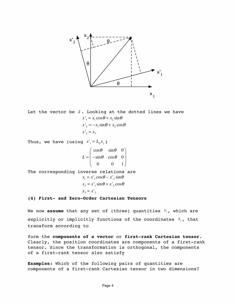
Let the vector be x . Looking at the dotted lines we have

x '1 = x1 cosθ + x2 sinθx '2 = −x1 sinθ + x2 cosθx '3 = x3

Thus, we have (using x 'i = Lij x j )

L =cosθ sinθ 0− sinθ cosθ 00 0 1

⎛

⎝

⎜⎜

⎞

⎠

⎟⎟

The corresponding inverse relations are

x1 = x '1 cosθ − x '2 sinθx2 = x '1 sinθ + x '2 cosθx3 = x '3

(4) First- and Zero-Order Cartesian Tensors

We now assume that any set of (three) quantities vi, which are

explicitly or implicitly functions of the coordinates xi , that transform according to

form the components of a vector or first-rank Cartesian tensor. Clearly, the position coordinates are components of a first-rank tensor. Since the transformation is orthogonal, the components of a first-rank tensor also satisfy

Examples: Which of the following pairs of quantities are components of a first-rank Cartesian tensor in two dimensions?

!

!

!

x

x

x'

x'

1

1

2

2

(i) Suppose (v1,v2 ) = (x2 ,−x1) are the components relative to the old axes.

We then have

v '1 = L11v1 + L12v2 = cosθ(x2 ) + sinθ(−x1) = x '2v '2 = L21v1 + L22v2 = − sinθ(x2 ) + cosθ(−x1) = −x '1

Thus, (v1,v2 ) = (x2 ,−x1) is a first-rank tensor.

(ii) Suppose (v1,v2 ) = (x2 , x1) are the components relative to the old axes.

We then have

v '1 = L11v1 + L12v2 = cosθ(x2 ) + sinθ(x1) ≠ x '2v '2 = L21v1 + L22v2 = − sinθ(x2 ) + cosθ(x1) ≠ x '1

Thus, (v1,v2 ) = (x2 , x1) is not a first-rank tensor.

(iii) Suppose (v1,v2 ) = (x12 , x2

2 ) are the components relative to the old axes.

We then have

v '1 = L11v1 + L12v2 = cosθ(x12 ) + sinθ(x2

2 ) ≠ x '12 = cosθ(x1) + sinθ(x2 )( )2

v '2 = L21v1 + L22v2 = − sinθ(x12 ) + cosθ(x2

2 ) ≠ x '22 = − sinθ(x1) + cosθ(x2 )( )2

Thus, (v1,v2 ) = (x12 , x2

2 ) is not a first-rank tensor.

Examples of first-rank tensors (vectors) are position, velocity, momentum, acceleration and force.

We now consider quantities that are unchanged by a rotation of the axes. They are called scalars or tensors or rank zero. They contain only one element. An example is the square of the distance of a point from the origin

r2 = x12 + x2

2 + x32

Under a transformation we get

r '2 = x '12+ x '2

2+ x '32 = r2

so the it is an invariant. We note that r2 is a scalar product, i.e., r2 =

x ⋅ x . It is easy to show that any scalar product

A ⋅B is

invariant under the transformation and is a tensor of rank zero.

A '⋅B ' = A 'i B 'i = LijAjLikBk = Lji

T LikAjBk = (LT L) jk AjBk = δ jkAjBk = AjBj =

A ⋅B

We can use a scalar to generate a tensor of rank one. Consider the new object (the gradient)

vi =∂φ∂xi

→ v = ∇φ

where φ is a scalar quantity. Under a rotation we get

v 'i =

∂φ∂xi

⎛⎝⎜

⎞⎠⎟

'=

∂φ '∂x 'i

=∂φ∂x 'i

=∂x j∂x 'i

∂φ∂x j

= Lij∂φ∂x j

= Lijvj

so we have constructed a first-rank tensor.

Now let us consider the quantity (the divergence)

s = ∇ ⋅ v =∂vi∂xi

where v is a first-rank tensor.

Under a rotation we get

s ' = ∂vi∂xi

⎛⎝⎜

⎞⎠⎟

'

=∂v 'i∂x 'i

=∂x j∂x 'i

∂v 'i∂x j

=∂x j∂x 'i

∂(Likvk )∂x j

= LijLik∂vk∂x j

= LjiT Lik

∂vk∂x j

= (LT L) jk∂vk∂x j

= δ jk∂vk∂x j

=∂vj∂x j

= s

so it is an invariant or zero rank tensor or scalar.

(5) Second- and Higher-Order Cartesian Tensors

We now define a second-rank Cartesian tensor as follows: the

elements Tij form the components of a second rank Cartesian tensor

if

T 'ij = LikLjlTkl and Tij = LkiLljT 'kl

Generalizing, we say that the elements Tij ....k form the components

of an nth rank Cartesian tensor (where n = the number of indices) if

T 'ij ...k = LipLjq .....LkrTpq....r and Tij ....k = LpiLqj .....LrkT 'pq....r

In 3 dimensions, an nth rank Cartesian tensor has 3n components.

Since a second-rank tensor has two indices, it is natural to

display its components in matrix form. The notation Tij⎡⎣ ⎤⎦ is used,

as well as T, to denote the matrix having Tij as the element in

the ith row and jth column. We also denote the column matrix

containing the elements vi of a vector by vi[ ].

We can think of a second rank tensor

T as a geometrical entity

and the matrix containing its components as a representation of the tensor with respect to a particular coordinate system.

Let us look more closely at the transformation rule for second rank tensors using its matrix representation. We have

T 'ij = LikLjlTkl = LikTklLjl = LikTkl (LT )lj

T ' = LTLT = LTL−1

Tij = LkiLljT 'kl = LkiT 'kl Llj = (LT )ijT 'kl Llj

T = LTT 'L = L−1T 'LThus, the matrix representing a second rank tensor behaves in the same way under orthogonal transformations as the matrix representation of a linear operator.

Not all linear operators, however, are second rank tensors.

Examples

(i) The outer product of two vectors. Let ui and vi , i = 1,2,3 be the components of two vectors (first rank tensors)

u and v and

consider the set of quantities Tij defined by

Tij = uivj

The set Tij are called the components of the outer product of

u and v . Under rotations the components of Tij become

T 'ij = u 'i v ' j = LikukLjlvl = LikLjlukvl = LikLjlTkl

which shows that they do transform as the components of a second rank tensor.

We denote the outer product, without reference to a coordinate system, by the symbol

T = u ⊗ v

This tells us the basis to which the components Tij of the second

rank tensor refer. Using

u = uiei and v = vieiwe have

T = uiei ⊗ vjej = uivjei ⊗ ej = Tijei ⊗ ej

Clearly, the quantities T 'ij are the components of the same tensor

T but referred to a different coordinate system, i.e.,

T = Tijei ⊗ ej = T 'ij e 'i⊗ e ' j

(ii) The gradient of a vector. Suppose that represents the components of a vector. We consider the quantities generated by

forming the derivatives of each vi , i=1,2,3, with respect to each

x j , j=1,2,3, i.e.,

Tij =

∂vi∂x j

We then have

T 'ij =

∂v 'i∂x ' j

=∂(Likvk )∂xl

∂xl∂x ' j

= Lik∂vk∂xl

∂xl∂x ' j

= Lik∂vk∂xl

Ljl = LikLjlTkl

which says that we have a second rank tensor

T = ∇v .

A test of whether any given set of quantities forms the components of a second rank tensor can always be made by direct

substitution of the x 'i in terms of the xi compared with using the transformation rule.

Example: Show that the elements Tij given by

T = Tij⎡⎣ ⎤⎦ =

x22 −x1x2

−x1x2 x12

⎛⎝⎜

⎞⎠⎟

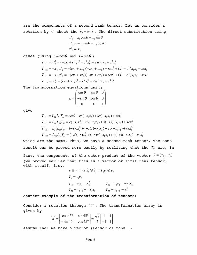
are the components of a second rank tensor. Let us consider a

rotation by θ about the e3 − axis . The direct substitution using

x '1 = x1 cosθ + x2 sinθx '2 = −x1 sinθ + x2 cosθx '3 = x3

gives (using c = cosθ and s = sinθ )

T '11 = x '22 = (−sx1 + cx2 )

2 = s2x12 − 2scx1x2 + c

2x22

T '12 = −x '1 x '2 = −(cx1 + sx2 )(−sx1 + cx2 ) = scx12 + (s2 − c2 )x1x2 − scx2

2

T '21 = −x '1 x '2 = −(cx1 + sx2 )(−sx1 + cx2 ) = scx12 + (s2 − c2 )x1x2 − scx2

2

T '22 = x '12 = (cx1 + sx2 )

2 = c2x12 + 2scx1x2 + s

2x22

The transformation equations using

L =cosθ sinθ 0− sinθ cosθ 00 0 1

⎛

⎝

⎜⎜

⎞

⎠

⎟⎟

give

T '11 = L1kL1lTkl = ccx22 + cs(−x1x2 ) + sc(−x1x2 ) + ssx1

2

T '12 = L1kL2lTkl = c(−s)x22 + cc(−x1x2 ) + s(−s)(−x1x2 ) + scx1

2

T '21 = L2kL1lTkl = (−s)cx22 + (−s)s(−x1x2 ) + cc(−x1x2 ) + csx1

2

T '22 = L2kL2lTkl = (−s)(−s)x22 + (−s)c(−x1x2 ) + c(−s)(−x1x2 ) + ccx1

2

which are the same. Thus, we have a second rank tensor. The same

result can be proved more easily by realizing that the Tij are, in

fact, the components of the outer product of the vector

v = (x2 ,−x1)(we proved earlier that this is a vector or first rank tensor) with itself, i.e.,

v ⊗ v = vivjei ⊗ ej = Tijei ⊗ ejTij = vivjT11 = v1v1 = x2

2 T12 = v1v2 = −x1x2

T21 = v2v1 = −x1x2 T22 = v2v2 = x12

Another example of the transformation of tensors:

Consider a rotation through 45° . The transformation array is given by

a[ ] = cos45° sin 45°

− sin 45° cos45°⎡

⎣⎢

⎤

⎦⎥ =

22

1 1−1 1⎡

⎣⎢

⎤

⎦⎥

Assume that we have a vector (tensor of rank 1)

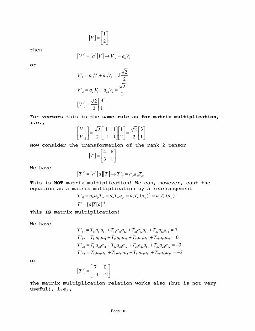
V[ ] = 1

2⎡

⎣⎢

⎤

⎦⎥

then

V '[ ] = a[ ] V[ ]→V 'i = aijVj

or

V '1 = a11V1 + a12V2 = 322

V '2 = a21V1 + a22V2 =22

V '[ ] = 22

31⎡

⎣⎢⎤

⎦⎥

For vectors this is the same rule as for matrix multiplication, i.e.,

V '1V '2⎡

⎣⎢

⎤

⎦⎥ =

22

1 1−1 1⎡

⎣⎢

⎤

⎦⎥12⎡

⎣⎢

⎤

⎦⎥ =

22

31⎡

⎣⎢⎤

⎦⎥

Now consider the transformation of the rank 2 tensor

T[ ] = 4 6

3 1⎡

⎣⎢

⎤

⎦⎥

We have

T '[ ] = a[ ] a[ ] T[ ]→ T 'ij = airajsTrsThis is NOT matrix multiplication! We can, however, cast the equation as a matrix multiplication by a rearrangement

T 'ij = airajsTrs = airTrsajs = airTrs (asj )T = airTrs (asj )

−1

T ' = [a]T [a]−1

This IS matrix multiplication!

We have

T '11 = T11a11a11 + T12a11a12 + T21a12a11 + T22a12a12 = 7T '12 = T11a11a21 + T12a11a22 + T21a12a21 + T22a12a22 = 0T '21 = T11a21a11 + T12a21a12 + T21a22a11 + T22a22a12 = −3T '22 = T11a21a21 + T12a21a22 + T21a22a21 + T22a22a22 = −2

or

T '[ ] = 7 0

−3 −2⎡

⎣⎢

⎤

⎦⎥

The matrix multiplication relation works also (but is not very useful), i.e.,

T '[ ] = a[ ] T[ ] a[ ]T =2

21 1−1 1⎡

⎣⎢

⎤

⎦⎥

4 63 1⎡

⎣⎢

⎤

⎦⎥

22

1 −11 1⎡

⎣⎢

⎤

⎦⎥

= 12

1 1−1 1⎡

⎣⎢

⎤

⎦⎥

10 24 −2

⎡

⎣⎢

⎤

⎦⎥ =

12

14 0−6 −4⎡

⎣⎢

⎤

⎦⎥ =

7 0−3 −2⎡

⎣⎢

⎤

⎦⎥

as expected.

(6) The Algebra of Tensors

Addition and Subtraction

If two tensors have the same rank, then they can be added and subtracted using their components

Sij ....k = Vij ....k +Wij ....k

Dij ....k = Vij ....k −Wij ....k

The new objects are tensors of the same rank.

Switching Indices

If a pair of indices are switched the new object is a tensor of

the same rank,i.e., if Vij ....k represents a tensor, then Vji....k

represents a tensor of the same rank.

If Vji....k = Vij ....k for all components, then Vij ....k is said to be symmetric

with respect to that pair of indices (or simply symmetric for

second rank tensors). If Vji....k = −Vij ....k for all components, then Vij ....k

s said to be antisymmetric with respect to that pair of indices (or simply antisymmetric for second rank tensors).

An arbitrary tensor is neither symmetric nor antisymmetric, but

can always be written as the sum of a symmetric tensor Sij ....k and

an antisymmetric tensor Aij ....k , i.e.,

Tij ....k =12

(Tij ....k + Tji....k ) + 12

(Tij ....k − Tji....k )

= Sij ....k + Aij ....kThe outer product discussed earlier is an example of a kind of "multiplication" of two tensors producing a tensor of higher rank. Our illustration had two first rank tensors producing a

second rank tensor. In general, the outer product of an nth rank tensor with an mth rank tensor produces an (n+m)th rank tensor.

We can produce a tensor of smaller rank from a tensor of larger rank using the contraction operation. The contraction operation consists of making two indices equal (and thus summing over that index). This reduces the number of indices (and hence the rank of the tensor) by two.

Example: Let Tij ..l ..m..k be the components of an nth rank tensor. This

implies that

T 'ij ..l ..m..k = LipLjq ......Llr .....Lms ....Lknn factors

Tpq....r ...s...n

If we contract on the indices l and m (set them both equal to l) we get

T 'ij ..l ..l ..k = LipLjq ......Llr .....Lls ....Lknn factors

Tpq....r ...s...n

= LipLjq ......δrs ....LknTpq....r ...s...n= LipLjq .......Lkn

(n−2) factors

Tpq....r ...r ...n

which says that the Tij ..l ..l ..k are the components of a different

Cartesian tensor of rank (n-2).

For a second rank tensor, the process of contraction is the same as taking the trace of the corresponding matrix. Therefore, the

trace Tii is a zero rank tensor (or scalar) and is invariant under rotations.

The scalar product or two vectors can be recast in tensor language as forming the outer product of two vectors (first rank

tensors) Tij = uivj and then contracting to form the scalar Tii = uivi

which is invariant under rotation as we found earlier.

Another familiar operation that is a special case of the contraction operation is the multiplication of a column vector

ui[ ] by a matrix Bij⎡⎣ ⎤⎦ to produce another column vector vi[ ], i.e.,

Biju j = vi

We can think of this as the contraction Tijj of the third rank

tensor Tijk formed from the outer product of Bij and uj .

(7) The Quotient Law

If we know that

B and

C are tensors and also that

Apq...k ...mBij ....k .....n = Cpq.....mij ...n

does this imply that the Apq...k ...m also form components of a tensor

A ?

Here

A ,B and

C are respectively of mth , nth and (m + n − 2)th rank. The

subscript k that has been contracted can be any of the

subscripts in

A and

B independently.

The quotient law states that if the above component relation

holds in all rotated coordinate systems, then the Apq...k ...m do form

the components of a tensor.

We will prove it for m = n = 2 only, but it should be clear that the principle of the proof holds for arbitrary m and n (just the algebra gets worse).

Suppose we start with

ApkBik = Cpi

where Bik and Cpi are arbitrary second rank tensors. Under a

rotation the set Apk (whether they are a tensor or not)

transforms to a new set A 'pk as follows

A 'pk B 'ik = C 'pi= LpqLijCqj = LpqLijAqlBjl

= LpqLijAqlLmjLnlB 'mn = LpqLijLmjLnlAqlB 'mn= Lpqδ imLnlAqlB 'mn= LpqLnlAqlB 'in

This can be rewritten (changing dummy index labels) as

(A 'pk− LpqLklAql )B 'ik = 0

Since Bik and hence B 'ik is an arbitrary tensor, we must have

A 'pk = LpqLklAql

which says that the Apk are the components of a second rank

tensor. The same result holds if we start with

ApkBki = Cpi

Using the quotient law to test whether a given set of quantities is a tensor is generally much more convenient than the direct substitution method we used earlier. A particular way in which it is applied is by contracting the given set of quantities, having n subscripts, with some arbitrary nth rank tensor and determining whether the result is a scalar.

Let us go back to an earlier example, namely,

T = Tij⎡⎣ ⎤⎦ =

x22 −x1x2

−x1x2 x12

⎛⎝⎜

⎞⎠⎟

The outer product xix j is a second rank tensor. Contracting it

with the Tij we get

Tij xix j = x22x1

2 − x1x2x1x2 − x1x2x2x2 + x12x2

2 = 0

which is clearly invariant. Thus, by the quotient theorem Tij must

also be a tensor. Very powerful!

(8) The Tensors δ ij and εijkSince

δ 'kl = LkiLljδ ij = LkiLli = δkl

δ ij is a second rank tensor.

Now consider the three-subscript Levi-Civita symbol εijk where we

have

εijk =+1 if i,j,k is an even permutation of 1,2,3−1 if i,j,k is an odd permutation of 1,2,3 0 other wise

⎧⎨⎪

⎩⎪

We then have

ε 'lmn = LliLmjLnkεijkBefore proceeding, we note that for a 3x3 matrix A, the

determinant A satisfies

A εlmn = AliAmjAnkεijkExample: Evaluate the determinant of the matrix

A =2 1 −33 4 01 −2 1

⎛

⎝

⎜⎜

⎞

⎠

⎟⎟

Setting l = 1, m = 2, and n = 3 we get

A ε123 = A = A1iA2 jA3kεijk = A11A22A33ε123 + A11A23A32ε132 + A12A21A33ε213 + A13A21A32ε312 + A12A23A31ε231 + A13A22A31ε321

= (2)(4)(1) − (2)(0)(−2) − (1)(3)(1) + (−3)(3)(−2) + (1)(0)(1) − (−3)(4)(1) = 35Now, using the above relation, we get

ε 'lmn = LliLmjLnkεijk = L εlmnSince L is orthogonal, its determinant is 1 and thus we have

ε 'lmn = εlmnThus, we have a third rank tensor.

These two tensors also have exactly the same components in every coordinate system.

Many of the familiar expressions of vector calculus can be

written as contracted tensors involving δ ij and εijk .

Examples:

(i)

a =b × c→ ai = εijkbjck

so that the cross-product produces a vector.

(ii)

a ⋅b = aibi = δ ijaibj

(iii)

∇2φ =

∂ 2φ∂xi∂xi

= δ ij∂ 2φ

∂xi∂x j(iv)

(∇ × v)i = εijk∂vk∂x j

(v)

∇(∇ ⋅ v)[ ]i =∂∂xi

∂vj∂x j

⎛

⎝⎜⎞

⎠⎟= δ jk

∂ 2vj∂xi∂xk

(vi)

∇ × (∇ × v)[ ]i = εijk∂∂x j

εklm∂vm∂xl

⎛⎝⎜

⎞⎠⎟= εijkεklm

∂ 2vm∂x j∂xl

(vii)

(a ×b) × c = δ ijciε jklakbl = εiklciakbl

An important identity between the ε and δ tensors is

εijkεklm = δ ilδ jm − δ imδ jl

This says that the two fourth rank tensors have identical components.

This allows us to find an alternative expression for

∇ × (∇ × v)[ ]i = εijkεklm∂ 2vm∂x j∂xl

= δ ilδ jm − δ imδ jl( ) ∂ 2vm∂x j∂xl

=∂ 2vj∂xi∂x j

−∂ 2vi

∂x j∂x j= ∇(∇ ⋅ v)[ ]i − ∇2vi

∇ × (∇ × v) = ∇(∇ ⋅ v) − ∇2vThat would be very cumbersome to prove using standard methods!

We can also show that

εijkε pqr =δ ip δ iq δ irδ jp δ jq δ jr

δkp δkq δkr

The identity we derive above is then a special case where (p, q, r) = (k, l, m). If we contract the identity by setting

j = l and using δkk = 3 we get

εijkεijm = 3δkm − δkm = 2δkm

and contracting once more by setting k = m we get

εijkεijk = 2δkk = 6

(9) Improper Rotations and Pseudotensors

The kind of transformations we have been discussing are called

proper rotations(where L = 1 ). Another kind of transformation is

called an improper rotation(where L = −1). In general, we consider this kind of transformation as a proper rotation plus an inversion of the coordinate axes through the origin represented by the equations

x 'i = −xi

An inversion changes a right-handed coordinate system into a left-handed coordinate system (proper rotations do not affect handedness). The matrix corresponding to the inversion transformation is

Lij = −δ ijA vector is a geometrical operator whose direction and magnitude are not affected by describing it in different coordinate systems (only it components change relative to new basis vectors). Therefore the components of a vector

v transform according to

v 'i = Lijvjunder all proper and improper rotations.

Let us now define another type of object whose components can also be labelled with a single index but which transforms as

v 'i = Lijvjunder proper rotations and as

v 'i = −Lijvjunder improper rotations. The new object is called a pseudotensor or pseudovector.

Pseudovectors should not be regarded as the same kind of geometrical object as a vector. Their directions are reversed under a transformation such as inversion as shown below.

In a similar way we can define scalars and pseudoscalars, where pseudoscalars are invariant under proper rotations but change sign under inversion (or reflection). We extend this to tensors of rank greater than 1.

In general, we write

T 'ij .....k = LilLjm ...LknTlm,,,,,n for tensors

T 'ij .....k = L LilLjm ...LknTlm,,,,,n for pseudotensors

For example, earlier we found that

L εijk = LilLjmLknεlmn

Since L = ±1 we can write this as

εijk = L LilLjmLknεlmn

Therefore, εijk is a third rank Cartesian pseudotensor. Now

consider the cross- or vector-product a =b × c where

b and c re

vectors. We then have

ai = εijkbjck

Under a transformation, we write

a 'i = ε 'ijk b ' j c 'k = L LilLjmLknεlmnLjpbpLkqcq = L LilLjmLjpLknLkqεlmnbpcq = L Lilδmpδnqεlmnbpcq = L Lilεlmnbmcm = L Lilai

which says that the cross-product is a pseudovector (not a vector!).

Now the quantities ai = εijkbjck are the components of the physical

vector a =b × c provided we are using a right-handed Cartesian

coordinate system. However, in a different coordinate system,

which is left-handed, the quantities a 'i = ε 'ijk b ' j c 'k are not the

components of the physical vector a =b × c which has, instead,

the components −a 'i .

It is very important to note the handedness of a coordinate system before setting out to write in component form the vector

relation a =b × c .

The kind of transformations we have been using are called passive transformations. In passive transformations, the physical system is left unchanged and only the coordinate system used to describe it is changed. In active transformations, the system itself is altered.

As an example, let us consider a particle of mass m that is located at a position

x relative to the origin O and hence has a

velocity x . The angular momentum of the particle about O is thus

J = m(x × x).

If we merely invert the Cartesian coordinates used to describe the system through the origin O, neither the magnitude nor direction of the vectors will be changed since they may be considered simply as arrows in space that are independent of the coordinates used to describe them. If we perform an active transformation such as inverting the position vector through O, then particle velocity is also reversed (it is the time derivative of the position vector). The angular momentum vector, however, remains unaltered.

This suggests that vectors can be divided into two categories as follows: polar vectors (such as position and velocity), which reverse under an active inversion of the physical system through the origin O and axial vectors (such as angular momentum) that remain unchanged. Note that we have specifically not introduced the concept of a pseudovector to describe a physical quantity.

(10) Dual Tensors

Consider a second rank pseudotensor Aij (in three dimensions).

For every such object, we construct the object

pi =

12εijkAjk

which is called the dual of Aij . It is a pseudovector. If we denote the antisymmetric tensor by the matrix

Aij⎡⎣ ⎤⎦ =0 A12 −A31

−A12 0 A23A31 −A23 0

⎛

⎝

⎜⎜

⎞

⎠

⎟⎟

then the components of the dual pseudovector are

(p1, p2 , p3) = (A23,A31,A12 )We also have result

εijk pk =

12εijkεklmAlm =

12(δ jlδkm − δ jmδkl )Alm = Aij

riley,hobson,bence: mathematical methods - · pdf filetensors! [these notes taken from...

Documents