riparian marshland composition and productivity …

RIPARIAN MARSHLAND COMPOSITION AND PRODUCTIVITY MAPPING

USING IKONOS IMAGERY

By

Kristie A. Dillabaugh, BES (Hons.)

A thesis submitted to

the Faculty of Graduate Studies and Research

in partial fulfilment of the requirements of the degree of

Master of Science

Department of Geography and Environmental Studies

Carleton University

Ottawa, Ontario

September, 2006

© Kristie Dillabaugh, 2006

Reproduced with permission of the copyright owner. Further reproduction prohibited without permission.

Library and Archives Canada

Bibliotheque et Archives Canada

Published Heritage Branch

395 Wellington Street Ottawa ON K1A 0N4 Canada

Your file Votre reference ISBN: 978-0-494-18360-1 Our file Notre reference ISBN: 978-0-494-18360-1

Direction du Patrimoine de I'edition

395, rue Wellington Ottawa ON K1A 0N4 Canada

NOTICE:The author has granted a nonexclusive license allowing Library and Archives Canada to reproduce, publish, archive, preserve, conserve, communicate to the public by telecommunication or on the Internet, loan, distribute and sell theses worldwide, for commercial or noncommercial purposes, in microform, paper, electronic and/or any other formats.

AVIS:L'auteur a accorde une licence non exclusive permettant a la Bibliotheque et Archives Canada de reproduire, publier, archiver, sauvegarder, conserver, transmettre au public par telecommunication ou par I'lnternet, preter, distribuer et vendre des theses partout dans le monde, a des fins commerciales ou autres, sur support microforme, papier, electronique et/ou autres formats.

The author retains copyright ownership and moral rights in this thesis. Neither the thesis nor substantial extracts from it may be printed or otherwise reproduced without the author's permission.

L'auteur conserve la propriete du droit d'auteur et des droits moraux qui protege cette these.Ni la these ni des extraits substantiels de celle-ci ne doivent etre imprimes ou autrement reproduits sans son autorisation.

In compliance with the Canadian Privacy Act some supporting forms may have been removed from this thesis.

While these forms may be included in the document page count, their removal does not represent any loss of content from the thesis.

Conformement a la loi canadienne sur la protection de la vie privee, quelques formulaires secondaires ont ete enleves de cette these.

Bien que ces formulaires aient inclus dans la pagination, il n'y aura aucun contenu manquant.

i * i

CanadaReproduced with permission of the copyright owner. Further reproduction prohibited without permission.

Abstract

The Ontario Wetland Evaluation System (OWES) employs a visual assessment

of wetland extent, composition and biomass as primary indicators in determining

which wetlands should be considered provincially significant and subsequently

protected. High resolution satellite remote sensing offers the potential to provide

more quantitative analysis at greater spatial detail within a given wetland using

spectral and spatial image information. In this study, Ikonos imagery was used to

map vegetation composition and productivity in three riparian marshes located

along the Rideau River near Ottawa, Ontario. Separability and correlation

analyses aided in the selection of an optimum set of spectral and spatial data,

which were used in classification tests, with training and validation data being

randomly selected from a set of 107 field sites. Terrestrial and aquatic

vegetation was classified comparing maximum likelihood (ML) and neural

network classifications, with a ML classification using a Transformed Vegetation

Index (TVI), visible bands, A2M5grn and CON5nir textures resulting in the

highest accuracy of 88% and a Khat statistic of 0.72. For biomass mapping, a 1

m2 sample frame was used to collect green and senescent vegetation at 75

locations within the various vegetation classes. Dry biomass was modelled

against the spectral and textural image measures using forward stepwise

regression. Log green biomass modelled by a combination of texture and

spectral variables provided the best result. The absolute error of this model in

predictive biomass mapping was 213 g/m2 or approximately 40% of the mean

field measured biomass.

i i


Acknowledgements

This has been a long and challenging journey and I have been blessed with a lot

of help from many wonderful people.

I would first like to thank my supervisor, professor Douglas King, for his patience

when this research was delayed and slow to progress. He has encouraged

independent thought and development of my research ideas, from the very

beginning, and has guided the development and progression of those ideas. As

a result, I have gained tremendous experience in the processes of research

design and development. I am also thankful for the financial support he has

given me especially during the last two years when progress has been especially

sluggish.

Secondly, I would like to thank professor Mike Pisaric for providing me with

excellent TA work experiences, for allowing me to use his refrigerator to store my

LARGE quantities of vegetation, and for being approachable and kind enough to

listen whenever I needed to talk.

I believe I am the last to graduate out of those that began this journey with me

and it has been difficult to finish this journey alone. The one person that is still

around is my great friend RAVS. You have braved the wetland with me and were

the most outstanding field assistant I could ever have had. It was hard work and

never once did you complain. You spent countless hours in the lab chopping,

i i i


weighing and drying vegetation, and helping me edit my final draft and I could not

have completed this research without you. I am, however, most appreciative of

your friendship, it has meant the world to me over the last few years.

I would also like to thank my family who has endured this experience with me.

Special thanks firstly to my momma who has often helped me by taking care of

baby Eden so I could work on my thesis. I believe one of the greatest things you

have ever taught me is to never quit...finish what you start! You have sacrificed

so much for me and I am grateful that you have always been there for me (even

when we share the same roof). Despite the severe allergic reaction to Common

cattail (Typha latifolia) and the subsequent day’s delay in collecting field data I’m

so grateful for my brother Drew and for the encouragement he has given me. A

HUGE thank-you also goes to Sondra and Derlin for taking care of Eden when I

had deadlines to meet finishing this work. I would also like to thank Binga and

Reegan for being like another set of parents for me and grandparents for Eden.

A BIG thank-you to my wonderful friend Heather for being such a shining

example to me I could always call for help when I needed somewhere for Eden to

play, we’ll miss you guys TONS!

I would be remiss if I didn’t thank Hazel Anderson for being so supportive and

encouraging over the last four years. Has it really been four years? Hazel is the

most helpful graduate secretary I’ve ever known! Robby Bemrose began my

field work with me and I’m thankful for his help in selecting my field plots and

iv


helping me traverse the wetlands. My regression analysis couldn’t have been

accomplished without Jon Pasher’s condensed SPSS course-THANKS!

Professor Scott Mitchell provided me with valuable information on the collection

and processing of biomass, and contributed insight during the final editing stage

of this thesis (thank-you so much for your contributions).

Second to last I would like to thank Craiger for encouraging me to finish this

insurmountable task. You have been my personal technical support line, my

extra field assistant, and my best friend and I couldn’t have done this without you.

Thank you for being patient and understanding when life was tough.

Lastly I would like to thank baby Eden, who interrupted this research process, for

being my ray of sunshine, for making me laugh and reminding me of the true

blessings in life. I just hope you learn how to SLEEP soon!

I would like to dedicate this thesis to baby Eden. Despite the difficulties

associated with having children and completing a graduate degree I wouldn’t

trade you for anything in the world!

v


Table of Contents

Abstract......................................................................................................................ii

Acknowledgements................................................................................................ iii

Table of Contents................................................................................................... vi

List of Tables........................................................................................................... ix

List of Figures........................................................................................................... x

List of Acronyms.................................................................................................... xi

Chapter One: Introduction..................................................................................... 1

1.1 Research Objectives.....................................................................................21.2 Thesis Structure............................................................................................3

Chapter Two: Background.....................................................................................5

2.1 Wetlands Introduced.....................................................................................52.1.1 Wetland Types.........................................................................................62.1.2 Wetland Importance...............................................................................112.1.3 Wetland Distribution and Disturbance.................................................. 12

2.2 Classification of Wetland Composition................................................... 132.2.1 Sensor Data Types.................................................................................15

2.2.1.1 Moderate Resolution Sensors........................................................ 152.2.1.2 High Resolution Sensors................................................................162.2.1.3 Radar Systems................................................................................17

2.2.2 Image Data Transformations used in Classification............................182.2.2.1 Vegetation Indices.......................................................................... 182.2.2.2 Texture.............................................................................................222.2.2.3 Principal Component Analysis...................................................... 26

2.2.3 Wetland Vegetation Classification........................................................ 272.2.3.1 Unsupervised Classification........................................................... 272.2.3.2 Supervised Classification............................................................... 272.2.3.3 Artificial Neural Networks............................................................... 28

2.2.4 Accuracy Assessment o f Classified Maps............................................292.2.5 Previous Wetland Classification Studies..............................................30

2.2.5.1 Previous Wetland Studies using Moderate Resolution OpticalImagery..................................................................................................... 312.2 5.2 Wetland Studies using High Resolution Imagery.....................33

2.2.5.3 Use of Vegetation Indices in Image Classification....................... 352.2.5.4 Use of Texture in Image Classification......................................... 36

v i


2.2.5.5 Use of Principal Components in Image Classification.................. 382.2.5.6 Studies using Unsupervised Classification................................... 392.2.5.7 Studies using Supervised Classification....................................... 402.2.5.8 Studies using Neural Networks...................................................... 41

2.3 Biomass and Cover Modelling................................................................. 422.3.1 Forward Stepwise Regression.............................................................. 432.3.2 Assessment of Model Quality and Predictive Accuracy...................... 442.3.3 Previous Biomass and Cover Modelling Studies.................................46

2.3.3.1 Use of Vegetation Indices in Biomass and Cover Modelling 472.3.3.2 Use of Texture in Biomass Modelling............................................ 492.3.3.3 Use of Principal Components in Biomass Modelling.................... 49

Chapter Three: Methods......................................................................................51

3.1 Study Area....................................................................................................513.2 Selection of Field Plots and Field Sampling Methods......................... 53

3.2.1 Field Sampling for Image Classification of Wetlands............................533.2.2 Field Sampling for Biomass and Cover Modelling...............................57

3.3 Ikonos Data Acquisition............................................................................ 603.4 Image Georeferencing............................................................................... 613.5 Image Data Transformations.....................................................................62

3.5.1 Vegetation Indices................................................................................. 623.5.2 Texture Analysis.................................................................................... 623.5.3 Principal Component Analysis.............................................................. 63

3.6 Wetland Vegetation Classification.......................................................... 643.6.1 Separability Analysis.............................................................................. 643.6.2 Maximum Likelihood Classification....................................................... 653.6.3 Neural Network Classification............................................................... 663.6.4 Classification Accuracy Assessment....................................................69

3.7 Biomass and Cover Modelling................................................................. 693.7.1 Biomass Model Assessment and Validation........................................ 71

Chapter Four: Results..........................................................................................72

4.1 Principal Component Analysis................................................................724.2 Separability Analysis.................................................................................73

4.2.1 Spectral Bands versus Principal Components..................................... 744.2.2 Determining the Best Texture Variables for Classification.................. 764.2.3 Determining Appropriate Vegetation Indices for Classification...........774.2.4 Merging Wetland Classes based on Separability................................78

4.3 Classification Analysis.............................................................................. 794.3.1 Maximum Likelihood Classification...................................................... 80

4.3.1.1 Classification using Seven Classes................................................ 804.3.1.2 Classification using Six Classes..................................................... 83

v ii


4.3.1.3 Classification using Five Classes.................................................. 874.3.2 Summary of Classification Results....................................................... 914.3.3 Additional Maximum Likelihood Classifications................................... 944.3.4 Neural Network Classification................................................................97

4.4 Biomass and Cover Modelling............................................................... 1004.4.1 Biomass Modelling............................................................................ 100

4.4.1.1 Biomass Model Assessment and Validation..............................1044.4.1.2 Cover Modelling.............................................................................106

Chapter Five: Discussion and Conclusions ...........................................110

5.1 Data Collection.......................................................................................... 1105.2 Wetland Vegetation Classification........................................................ 1115.3 Biomass and Cover Modelling................................................................1165.4 Overall Conclusions.................................................................................119

References.............................................................................................................122

V lll


List of Tables

Table 1. Correlation matrix (showing r values) for Ikonos spectral bands 63Table 2. Neural network configurations..................................................................68Table 3. Variations for biomass regression analysis............................................. 70Table 4. PCA of spectral data: Factor loadings table............................................72Table 5. Separability results for different combinations of spectral bands and 7

classes...................................................................................................... 74Table 6. Separability results for spectral bands and PCs combined with A2M5grn

and CON5nir with varying number of wetland classes..........................75Table 7. Separability results for selected 3 x 3 and 5 x 5 textures based on 7

classes...................................................................................................... 76Table 8. Individual textures showing highest separability based on 7 classes. . 77 Table 9. Separability results for top three data combinations for 7, 6 and 5

wetland classes based on 50% training 3x3 clusters............................79Table 10. Error matrix for 7 class MSAVI classification.......................................80Table 11. Producer and user accuracies for 7 class MSAVI classification........ 82Table 12. Error matrix for 6 class TVI classification.............................................84Table 13. Producer and user accuracies for 6 class TVI classification.............. 85Table 14. Error matrix for 5 class Spectral bands, A2M5grn and CON5nir

classification.......................................................................................... 88Table 15. Producer and user accuracies for 5 class spectral bands, A2M5grn

and CON5nir classification................................................................... 89Table 16. Number of pixels per wetland class for 5 classes using approximately

50% training and 50% validation 3 x 3 clusters.................................. 93Table 17. Error matrix for 5 class TVI classification.............................................. 95Table 18. Producer and user accuracies for 5 class map derived from TVI

classification.......................................................................................... 96Table 19. Neural network convergence..................................................................98Table 20. Error matrix for 5 class neural network (#14) classification................. 99Table 21. Producer and user accuracies for 5 class map derived from neural

network (#14).........................................................................................99Table 22. Variance accounted for by models of total combined biomass, total

green biomass and total senescent biomass....................................101Table 23. F?2 contribution of independent variables in log green biomass model.

102Table 24. Single variable model validation results.............................................. 105Table 25. Multiple variable model validation results............................................105Table 26. Comparing field estimates and calculated estimates of percent cover.

108Table 27. Variance accounted for by models of aquatic green field cover 108

ix


List of Figures

Figure 1. Bog wetland type...................................................................................... 7Figure 2. Fen wetland type.......................................................................................8Figure 3. Swamp wetland type................................................................................ 8Figure 4. Marsh wetland type.................................................................................10Figure 5. Shallow open water environment...........................................................10Figure 6. Study Area:..............................................................................................53Figure 7. Emergent terrestrial vegetation..............................................................56Figure 8. Shrub vegetation.....................................................................................56Figure 9. Aquatic vegetation.................................................................................. 57Figure 10. Grasses/sedges and forest vegetation.................................................57Figure 11. Terrestrial and Aquatic Field Plots........................................................58Figure 12. Drying Curve for green floating aquatic vegetation......................... 59Figure 13. Drying curve for green emergent terrestrial vegetation...................60Figure 14. MSAVI classification for 7 classes with mode filter applied................82Figure 15. TVI classification for 6 classes with mode filter applied......................86Figure 16. Spectral band classification for 5 classes with mode filter applied... 89Figure 17. Emergent aquatic vegetation................................................................ 90Figure 18. Emergent terrestrial versus emergent aquatic vegetation..................93Figure 19. TVI classification for 5 classes with mode filter applied.....................96Figure 20. Neural Network 14 for five wetland classes....................................100Figure 21. Gradient map of biomass....................................................................103Figure 22. Biomass map showing three levels of biomass.................................104Figure 23. Floating aquatic plot and corresponding classified image................ 107Figure 24. Emergent aquatic plot and corresponding classified image............. 107

x


List of Acronyms

A2M Angular Second Moment texture measureA2M5grn Angular Second Moment texture measure derived from green b£

using 5 x 5 window sizeA2M5nir Angular Second Moment texture measure derived from near

infrared band using 5 x 5 window sizeAGB Above Ground BiomassAIRSAR Airborne Imaging Radar Synthetic Aperture RadarANN Artificial Neural NetworkARVI Atmospherically Resistant Vegetation IndexASVI Atmospheric and Soil Vegetation IndexATLAS Airborne Terrestrial Applications SensorAVHRR Advanced Very High Resolution RadiometerBD Bhattacharrya DistanceCASI Compact Airborne Spectrographic ImagerCON Contrast texture measureCON5nir Contrast texture measure derived from near infrared band using

5 x 5 window sizeCOR Correlation texture measureDIS Dissimilarity texture measureDN Digital NumberDVI Differenced Vegetation IndexEM Emergent Terrestrial vegetation classEMAQ Emergent Aquatic vegetation classENTR Entropy texture measureERS-1 European Remote Sensing SatelliteFLAQ Floating Aquatic vegetation classFOR Forest vegetation classGEMI Global Environmental Monitoring IndexGLA2M GLDV Angular Second Moment texture measureGLCM Grey level co-occurrence matrixGLCON GLDV Contrast texture measureGLDV Grey level difference vectorGLENTR GLDV Entropy texture measureGLMN GLDV Mean texture measureGPS Global Positioning SystemGS Grasses/Sedges vegetation classGVI Green Vegetation IndexHOM Homogeneity texture measureHRV High Resolution VisibleIRS Indian Remote Sensing SatelliteKhat Kappa StatisticLISS Linear Self Scanning SensorMIR Mid infrared

x i


ML Maximum Likelihood classifierMN Mean texture measureMN3nir Mean texture measure derived from near infrared band using 3 x 3

window sizeMN5grn Mean texture measure derived from green band using 5 x 5 window

sizeMN5nir Mean texture measure derived from near infrared band using 5 x 5

window sizeMSAVI Modified Soil Adjusted Vegetation IndexMSS Multispectral ScannerNAD North American DatumNDVI Normalized Difference Vegetation IndexNIR Near infraredOMNR Ontario Ministry of Natural ResourcesOW Open Water classOWES Ontario Wetland Evaluation Systemp statistical significancePAN PanchromaticPC Principal ComponentPCA Principal Component AnalysisPCI Image processing softwareR2 Coefficient of determinationR2adj Adjusted coefficient of determinationRMS Root mean squareRMSE Root mean square errorRVI Ratio Vegetation IndexSAVI Soil Adjusted Vegetation IndexSe Standard error of the estimateSHR Shrub vegetation classSPOT Systeme pour (’Observation de la TerreSTDEV Standard Deviation texture measureTERm Terrestrial Marsh vegetation classTEX TextureTIR Thermal infraredTM Landsat Thematic MapperTSAVI Transformed Soil Adjusted Vegetation IndexTVI Transformed Vegetation IndexUTM Universal Transverse Mercator projectionVI Vegetation IndicesVIF Variance Inflation Factor

x i i


Chapter One: Introduction

Vegetation plays a key ecological role within all wetland environments. Marshes,

chosen as the focal wetland type for this research, are dominated by emergent

and aquatic vegetation, although peripheral trees and low shrubs also occur.

Due to increased pressures on wetlands from urbanization and agriculture, it has

become necessary to develop protection policies, which have in turn initiated the

development of an evaluation system within Ontario to identify priority wetlands

for protection. The purpose of the Ontario Wetland Evaluation System (OWES)

is to rate the potential significance of a wetland based on four components

including hydrology, biology, social benefits and special features. The

assessment of wetlands by the OWES is conducted on the ground with the aid of

air photos and existing maps. These methods typically introduce observer bias

and are labour intensive for large wetlands. Field investigations are generally

very expensive and access to wetland environments is often difficult due to

uneven and unstable terrain, tall vegetation and deep water.

Remote sensing technology can be used to identify wetland type, extent, spatially

associated resources and vegetation communities (Lyon and McCarthy, 1995).

Though moderate resolution imagery has been used extensively for regional

wetland mapping applications it has not been successfully used for detailed

wetland mapping. With higher resolution capabilities remote sensing offers a

unique way to identify and map vegetation composition and structure associated

with riparian wetlands which are often narrow and linear in form. This type of

1


image data could allow for greater attribute precision, so that smaller vegetation

classes and wetland boundaries would be more easily detectable. Thematic

land-cover maps derived from satellite image classification techniques can aid in

the analysis of spatial patterns and help identify unevaluated wetland areas that

are susceptible to development and agricultural pressures.

Remote sensing has traditionally been used as a tool for land use and land cover

mapping, though increasingly it is being used for collecting biophysical

information such as vegetation and soil moisture contents, percent vegetation

cover and vegetation biomass. Multispectral satellite imagery can be analysed to

produce distribution maps per unit area that are useful for modelling plant stress

and yield (Jensen, 1983). Typically, a relation between spectral data or

transformations such as vegetation indices and biomass is developed for sample

data using regression-based methods and the regression equation is applied to

other non-sampled areas to produce biomass maps (Campbell, 1996).

1.1 Research Objectives

There were two primary objectives to this research:

1) To determine if Ikonos imagery can be used to map riparian marsh

vegetation composition.

2) To model biomass and cover within riparian marsh wetlands.

2


Associated with the first objective was a need to determine the best combination

of image inputs for use in a comparison of a traditional supervised classification

technique versus a neural network approach and to evaluate the accuracy of

classified maps using separate validation data not input to the classification

process.

For the second objective harvested biomass in g/m2 was used as the dependent

variable in forward stepwise regression against image variables, including raw

spectral bands, vegetation indices, textures and principal components, to

determine the best predictors of biomass. The best biomass model was

validated and accuracy was assessed.

1.2 Thesis Structure

This thesis is organized into six chapters. Chapter one introduces the

importance of wetland mapping and modelling, defines the research objectives,

and outlines the structure of the thesis. Chapter two gives the background

information for this research derived from the literature including: an introduction

to wetlands, descriptions of data transformations, classification techniques and

accuracy assessment used in this thesis, and a discussion of techniques for

modelling wetland biomass and vegetation cover and for model assessment.

Chapter three describes the study area, explains methods used for field plot

selection and field sampling techniques, discusses image acquisition and data

processing for wetland classification and accuracy assessment, and finally

3


reviews biomass and cover modelling techniques and model validation and

assessment used in this research. The results for wetland classification and

modelling are presented in Chapter four. Chapter five situates the major findings

of this research in relation to the literature, discusses significant contributions and

recommendations for future research, and finally outlines the overall conclusions

of this research.

4


Chapter Two: Background

2.1 Wetlands Introduced

Wetlands are transitional zones located between terrestrial and aquatic

ecosystems, which experience seasonal or permanent above surface water. As

a result, saturated soils and hydrophytic (water tolerant) vegetation predominate.

Defining wetland environments, however, has long been a challenge. Wetlands

are not static systems, as they undergo natural succession, experience

fluctuating water levels and vary in form and process with differences in size and

location. Formal wetland definitions have been developed by many agencies in

the United States and Canada and through an international treaty known as the

Ramsar convention (Mitsch and Gosselink, 1993). The Ramsar convention was

initially adopted at an international conference in Ramsar, Iran in 1971. The

global treaty provides the framework for the international protection of wetlands

that provide habitat for migratory birds. Wetland definitions can be used for both

scientific and management purposes (Mitsch and Gosselink, 2000). In Canada

wetlands are formally defined as, "land that is saturated with water long enough

to promote wetland or aquatic processes as indicated by poorly drained soils,

hydrophytic vegetation which is periodically deficient in oxygen and various kinds

of biological activity adapted to a wet environment" (National Wetlands Working

Group Canada Committee on Ecological Land Classification, 1988, p.416).

5


2.1.1 Wetland Types

There are five major wetland types recognized and defined in Canada by the

National Wetlands Working Group (1988): bogs, fens, swamps, marshes and

shallow open water. Wetlands are organized into these five types as each one

exhibits a unique form, has varying relative primary productivity rates and

provides habitat to different animals and plants (Ontario Ministry of Natural

Resources, 1993).

Bogs are most commonly found in northern Canada where peat accumulation

exceeds 40 cm in depth. Bogs have a high water table and contain vegetation

adapted to nutrient poor conditions. The bog surface is often raised and isolated

from mineralized soils, but remains flat or level with the surrounding wetlands.

As a result, the surface water of bogs is extremely acidic and the upper layers

are nutrient deficient, which results in poor plant diversity. Bogs are typified by

sphagnum moss and ericaceous shrub vegetation such as leatherleaf

(Chamaedaphne calyculata) and bog laurel (Kalmia polifolia). Black spruce

(P/'cea mariana) is the dominant tree found within bogs though tree cover does

not exceed 25%. Figure 1 shows a typical northern bog environment.

6


Figure 1. Bog wetland type.www.aquatic.uoquelph.ca/wetlands/chapter2/boqs.htm; Hebert PDN (2002a).

Fens are peatlands that have a high water table but very slow internal drainage,

as a result of low gradient slopes. The oxygen level is low and mineral supply is

limited. Plant diversity is higher in fens than in bogs with sedges as the

predominant vegetation community, though mosses, vascular plants, shrubs and

sparse trees are also found. Sedge species such as creeping sedge (Carex

chordorrhiza), livid sedge (Carex livida) and candle lantern sedge (Carex limosa),

and a shrub known as bog willow (Salix pedicellaris) are considered to be

common fen indicator species (Newmaster et al., 1997). Tree species such as

white cedar (Thuja occidentalis L.) and tamarack (Larix laricina) less than 6

metres in height are common. Within fen communities vascular plant species

such as pitcher plant (Sarracenia purpurea) and buckbean (Menyanthes trifoliata)

are often found. A fen environment is shown in Figure 2.

7


http://www.aquatic.uoquelph.ca/wetlands/chapter2/boqs.htm

Figure 2. Fen wetland type.www.aquatic.uoquelph.ca/wetlands/chapter2/fens.htm; Hebert PDN (2002b).

A swamp has trees and tall shrubs (>6 metres in height) that dominate at least

25% of the area and the subsurface is continuously waterlogged as a result of

standing or gently moving water. The water table may drop seasonally below the

vegetation root zone, creating aerated conditions at the surface. Swamp waters

are neutral to moderately acidic and show little deficiency in oxygen or mineral

nutrients. Treed swamps may have either deciduous or coniferous species such

as silver maple (Acer saccharinum), black ash (Fraxinus nigra), yellow birch

(Betula alleghaniensis), and black spruce (Picea mariana). Thicket swamps are

dominated by shrub species such as dogwood (Cornaceae spp.) and speckled

alder (Alnus rugosa). A typical treed swamp environment is shown in Figure 3.

Figure 3. Swamp wetland type.www.aquatic.uoquelph.ca/wetlands/chapter2/swamps.htm; Hebert PDN (2002c).

8


http://www.aquatic.uoquelph.ca/wetlands/chapter2/fens.htm

http://www.aquatic.uoquelph.ca/wetlands/chapter2/swamps.htm

Marshes are nutrient rich areas that are periodically inundated by standing or

slow moving water. Wet mineral soil areas predominate, but shallow well

decomposed peat may be present. They are subject to a fluctuating water table,

but water remains within the plant rooting zone for most of the growing season.

Waters are usually neutral to slightly alkaline, with high oxygen levels. Tall

emergent vegetation such as common cattail (Typha latifolia) and common reed

(Phragmites australis) predominate, although low shrubs such as sweet gale

(Myrica gale) and red osier dogwood (Cornus stolonifera) are commonly found

while tree species such as black ash (Fraxinus nigra) often form the periphery.

Broad leaved plants such as Sagittaria spp. and floating aquatic plants such as

fragrant white water lily and yellow pond lily (Nymphaea odorata and Nuphar

variegatum) are also prevalent in open water areas. Ecologically, marshes are

considered as initial successional wetlands. If left undisturbed, marshes will

naturally succeed into swamps, while fens will succeed into bogs over many

years. As wetlands age, they become more sensitive to disturbance. A marsh

environment is shown in Figure 4 (one of the marshes of this study) with floating

aquatic vegetation and open water in the foreground and an abrupt vegetation

change to emergent vegetation in the background.

9


Figure 4. Marsh wetland type.

Shallow open waters are relatively small, non-fluvial bodies of standing water

representing a transitional stage between lakes or rivers and marshes (see

Figure 5). Submerged (Potamogeton spp.) and floating plants (Lemna spp.,

Spirodela spp., Wolffia spp., Nuphar and Nymphaea spp.) flourish in areas of

open water.

Figure 5. Shallow open water environment.www.aquatic.uoquelph.ca/wetlands/chapter2/shallow.htm; Hebert PDN (2002d).

10


http://www.aquatic.uoquelph.ca/wetlands/chapter2/shallow.htm

Riparian marshes were chosen as the wetland type for this research as they are

considered extremely productive environments and generally support several

vegetation communities including emergent terrestrial, shrub, grasses/sedges,

floating aquatic and emergent aquatic.

2.1.2 Wetland Importance

Wetlands provide many environmental functions such as playing a vital role in

the carbon cycle, as plants convert inorganic carbon into organic compounds

through the process of photosynthesis. Wetland plants also help to circulate

essential nutrients such as phosphorus and nitrogen, which are absorbed

through plant roots from soil and water and excreted as the plants and their

consumers die. As wetlands are typically located between terrestrial and aquatic

systems, they play an important role in regulating water flow. Water is absorbed

and temporarily stored when water levels are high and groundwater is recharged

by wetlands during drier periods. Water quality improvement is also another

important function of wetlands, as they act as natural filters, with wetland plants

removing sediments and debris from the water and absorbing nutrients and

heavy metals. Soil erosion is reduced as wetland plant root systems act as

stabilising agents. Wetlands are highly productive ecosystems and therefore

provide habitat for many plant and animal species. Plant nutrients can be utilized

by wetland wildlife forming the basis of complex food chains (Twolan-Strutt,

1995; Mitsch and Gosselink, 1993; Larson and Newton, 1981; Lewis, 2001;

Williams, 1990; Hammer, 1997).

11


The physiographic position of a wetland within a landscape is an important

ecological factor in determining its function, importance and productivity.

Riparian wetlands are greatly influenced by adjacent rivers or streams and as a

result are typically linear in form and process large fluxes of energy and materials

from upstream systems (Mitsch and Gosselink, 2000). The productivity of

riparian wetlands has been found to increase with distance downstream from the

river mouth (Ontario Ministry of Natural Resources, 1994). Riparian wetlands are

particularly important for increasing riparian habitat and stabilizing river banks.

The preservation of shoreline vegetation and wetlands is critical for maintaining a

river's health and biodiversity.

2.1.3 Wetland Distribution and Disturbance

Wetlands can be found on every continent except Antarctica. According to

Mitsch and Gosselink (1993) approximately 6% or 8.6 million km2 of the earth’s

surface is wetland, with more than half of those being located in tropical and

subtropical regions, and the remaining wetlands being found primarily in boreal

and subarctic areas. Environment Canada (1986) indicated that 1.27 million km2

of Canada is covered by wetlands with the most extensive wetland concentration

occurring in the central provinces of Ontario and Manitoba.

Historically wetlands were regarded as wastelands having little or no value, yet

today they are recognized for their numerous ecological, hydrological and

recreational values. Wetland losses, however, have occurred in southern

12


Ontario since the time of settlement. By 1982, approximately 68% of the

wetlands in southern Ontario south of the Canadian Shield had been lost to

urbanization and agricultural expansion (Snell, 1987). Changes in wetland water

levels caused by urbanization can negatively influence wetland plants that are

adapted to specific water depths. As the ecology of a wetland is disturbed this

can have serious implications for the viability of the wetland itself (McBean et al.,

1996). Conversion of wetlands to other land uses by drainage, dyking and

infilling is typically irreversible. In addition to conversion for agriculture and urban

development, wetland types such as bogs and fens, which accumulate peat, are

often subject to intense peat extraction and subsequent drainage and

conversion. Due to these increased pressures on wetlands, it has become

necessary to develop protection policies, which have in turn initiated the

development of evaluation systems such as the OWES to identify priority

wetlands for protection.

2.2 Classification of Wetland Composition

Wetland mapping traditionally relied on extensive site investigations and analysis

of aerial photographs. These methods typically introduce observer biases and

can become extremely daunting tasks for large-area wetland studies. Field

investigations are generally very expensive and access to wetland environments

is often difficult due to uneven and unstable terrain, tall vegetation and deep

water.

13


Remote sensing offers the potential to provide spatially complete data coverage

of wetlands at any scale. Image based methods are also more suited to

temporal monitoring of wetlands than field based methods because such

methods can be standardized, alleviating the subjectivity caused by differences

between observers. Field based methods provide a horizontal perspective while

remote sensing provides a vertical view with less spatial distortion and more

detail in areas that would be far from the observer’s position, such as water and

vegetation hidden by taller vegetation. In addition, satellite images provide an

effective visual archive of temporal change that is not easily obtainable from field

assessment. Remote sensing technology is capable of detecting wetland extent,

identifying wetland type and their associated resources, and identifying

vegetation communities in a less intrusive manner than field surveys (Lyon and

McCarthy, 1995). Thematic land-cover maps derived from satellite image

classification techniques can aid in the analysis of spatial patterns and help

identify wetland areas that are susceptible to developmental and agricultural

pressures. Furthermore, land cover is an important determinant of species

abundance and diversity, with different species relying upon different vegetation

communities for cover and food (Griffiths et al., 1993).

The following subsections discuss the background to the data types and

classification methods used in this research, as well as previous wetland

classification studies.

14


2.2.1 Sensor Data Types

Satellite system characteristics such as spectral sensitivity and viewing capability

for moderate and high resolution sensors, and radar systems will be compared.

Some of the sensors that have successfully been used for wetland mapping will

be discussed.

2.2.1.1 Moderate Resolution Sensors

Satellite systems such as the Landsat Thematic Mapper (TM), Systeme pour

I’Observation de la Terre (SPOT), and the Indian Remote Sensing Satellite (IRS)

Linear Self-scanning sensor (LISS) operate in the optical portion of the spectrum

and are considered to be moderate resolution satellites. These sensors are

briefly summarized to provide context for the literature review on wetland

mapping that follows.

Landsat TM has 7 spectral bands; blue (0.45-0.52pm), green (0.52-0.60pm), red

(0.63-0.69pm), Near Infrared (NIR) (0.76-0.90pm), Mid Infrared (MIR) (1.55-

1.75pm), thermal (10.4-12.5pm) and MIR (2.08-2.35pm). The spatial resolution

is 30m for all bands except the thermal which is 120 m. When Landsat TM

imagery is used for wetland mapping bands 3 (red), 4 (NIR) and 5 (MIR) have

been found to be the best combination for wetland detection. The MIR band is

particularly important for discriminating between wetland types (Jensen et al.,

1993).

15


SPOT was the first earth observation satellite to have pointable off nadir viewing

capabilities. This satellite has 3 high resolution visible (HRV) bands sensing in

the green (0.50-0.59pm), red (0.61-0.68pm) and NIR (0.79-0.89pm) portions of

the spectrum with 20 m spatial resolution. In addition, SPOT panchromatic

(PAN) senses between 0.51-0.73pm and has a 10 m spatial resolution. SPOT-4

also has a MIR band (1.58-1.75pm) in addition to the other bands.

The IRS-1 B LISS-II system has four multispectral bands spectrally similar to

Landsat TM but with 72.5 m and 36.25 m spatial resolution.

When coarser resolution imagery is used to identify and delineate wetlands it has

generally been found that the use of multi-temporal data produces higher

accuracy but at greater cost (Ozesmi and Bauer, 2002; Ramsey and Laine, 1997;

Lunetta and Balogh, 1999).

2.2.1.2 High Resolution Sensors

In recent years a number of commercial high resolution satellites, such as

QuickBird and Ikonos, have been launched that provide spatial resolutions

approaching those of aerial photography. High resolution satellite imagery has

the ability to resolve greater detail such that smaller features on the ground are

identifiable in an image. This may specifically benefit wetland monitoring

applications, as spatial variations of vegetation species and structure as well as

small irregular patterns of degradation may be detectable from high resolution

16


imagery. Riparian wetlands are often narrow and linear in form and increased

resolution could allow for greater attribute precision, so that smaller vegetation

classes and wetland boundaries would be more easily detectable.

Ikonos and Quickbird each acquire multispectral imagery of approximately 4 m

resolution in the blue (0.45-0.52pm), green (0.52-0.60pm), red (0.63-0.69pm)

and NIR (0.76-0.90pm) portions of the spectrum, as well as panchromatic (0.45-

0.90pm) 1 m resolution data. They also have off nadir viewing capabilities unlike

most moderate resolution sensors. Despite the increased spatial resolution of

these sensors, however, they lack spectral detail, not having MIR or thermal

bands.

All of the above capabilities mentioned for moderate and high resolution sensors

are also available in airborne hyperspectral remote sensing with smaller pixel

sizes and greater numbers of bands. For example, the Compact Airborne

Spectrographic Imager (CASI) is a sensor allowing for the number and width of

spectral bands to be programmed with a minimum bandwidth of 2.6 nm.

2.2.1.3 Radar Systems

Radar systems transmit and receive radiation in the microwave portion of the

spectrum. They offer two advantages over optical sensors, including: 1) the

ability to acquire data at any time of day and under cloudy conditions; 2) radar

reflections or backscatter provide different information than optical data. For

17


Radarsat-1, depending on the beam mode or image size, different spatial

resolutions are achieved varying from 8 m to 100 m as the beam mode is varied

from fine to ScanSAR wide. With higher resolution satellite radar such as

Radarsat-2, or airborne radar, pixel size can be 3 m or less. Radar can detect

wetness and roughness related to vegetation structure and standing trees in

uniform wetland areas and can penetrate cloud cover (Kasischke and Bourgeau-

Chavez, 1997; Kushwaha et al., 2000; Austin et al., 2003; Sokol, 2003). It was,

however, not considered further because the spatial resolutions of satellite radar

are currently not fine enough for the highly detailed mapping requirements of this

research, and presently airborne radar imagery is very expensive.

2.2.2 Image Data Transformations used in Classification

Besides spectral data produced directly by each of the sensors, data

transformations are often used to produce additional or improved image

information for classification. The following subsections discuss the background

to transformations utilized in this research, including vegetation indices (VI),

texture analysis and Principal Component Analysis (PCA).

2.2.2.1 Vegetation Indices

A vegetation index is typically a specific formulation of spectral bands that

emphasizes the contrast between vegetation reflectance and reflectance of other

land cover types in different parts of the spectrum. Most commonly, they have

18


been derived from the red and near infrared due to the large contrast of

vegetation with soil and water in these bands, although some indices include the

blue, green or mid infrared.

This sub-section focuses on defining the vegetation indices that were used in this

research which include: Ratio Vegetation Index (RVI), Normalized Difference

Vegetation Index (NDVI), Transformed Vegetation Index (TVI), Differenced

Vegetation Index (DVI), Soil Adjusted Vegetation Index (SAVI), Modified Soil

Adjusted Vegetation Index (MSAVI), and Atmospheric and Soil Vegetation Index

(ASVI). Many other indices have been developed and evaluated but these were

deemed to be most relevant to this study.

The Ratio Vegetation Index (RVI), first proposed by Pearson and Miller (1972),

was one of the first ratio-based indices and was developed with the intent of

enhancing the contrast between bare ground and vegetation.

r v i = J L < 1 >

NIR

where, R is the reflectance in the red channel and NIR is the reflectance in the

near infrared channel.

NDVI was developed by Rouse (1973) and has become widely used because it

is computationally simple and is less sensitive to various illumination effects,

such as varying sun angle, slope and aspect (Lillesand and Kiefer, 2000).

19


NDVI =(njr - r)(NIR + R)

(2)

Ratio-based indices such as RVI and NDVI utilize the characteristic response of

vegetation in the red and near infrared portions of the spectrum, as shown by

chlorophyll absorption of vegetation in the red and high reflectance by vegetation

in the near infrared portions.

Perry and Lautenschlager (1984) proposed the formulation of the Transformed

Vegetation Index (TVI) to avoid the negative values resulting from the traditional

NDVI calculation.

where, NDVI is the normalized difference vegetation index.

The Differenced Vegetation Index (DVI) was developed by Clevers (1986) as

NDVI has been found to be sensitive to variations in soil reflectance in canopies

of less than 100% cover and to atmospheric variations, so modified indices have

been proposed (Eastwood et al., 1997). Those used in this research include: the

Soil Adjusted Vegetation Index (SAVI), the Modified Soil Adjusted Vegetation

Index (MSAVI) and the Atmospheric and Soil Vegetation Index (ASVI). Bare

soils and senescent vegetation have similar reflectance characteristics, so it was

hypothesized that these indices, which were developed primarily for agriculture,

^\NDVI + 0.5| (3)

DVI = (n IR -R ) (4)

20


might be useful for marsh wetlands where there are often large amounts of

senescent vegetation and/or exposed soil between the foliage and stalks of the

vegetation.

The Soil Adjusted Vegetation Index (SAVI) was developed by Heute (1988) and

is defined as

(N IR-R) (i + L) (5){NIR + R + L y ’

where, L is a soil adjustment factor. Huete (1988) found that L=0.5 minimized

the effects of soil background reflectance the best.

Qi et al. (1994a) proposed the Modified Soil Adjusted Vegetation Index (MSAVI)

to show that the adjustment factor L is not a constant but a function that varies

inversely with the amount of vegetation present (Bannari et al., 1995).

2NIR +1 - J(2NIR + 1)2 - 8(NIR - R) ^MSA VI = --------------^ -------------- V--------

The Atmospheric and Soil Vegetation Index (ASVI) developed by Qi et al.,

(1994b) is a modification of MSAVI and accounts for atmospheric scattering

effects by including the blue band in the formulation.

2NIR +1 - 7(2NIR + 1)2 - 8(NIR - 2 R + B) ^_ _

where, B is the reflectance in the blue channel.

21


2.2.2.2 Texture

Tone and texture are important recognition elements, which are used in the

process of image interpretation. Image tone can be described as the brightness

at a given point, as represented by a pixel in digital imagery, or as the average

brightness within a region. Texture is the spatial variation in brightness around a

given point (Arzandeh and Wang, 2002; Avery and Berlin, 1992). It is often

difficult to distinguish between a desired set of cover types based on pixel

intensity or tone alone, therefore, texture measures can be calculated and used

in the classification process.

Texture can be derived as a first order measure directly from the imagery (data

variance in a region) or as a second order measure derived from some

representation of pixel data variation. A popular second order data

representation used to calculate texture is the grey level co-occurrence matrix

(GLCM), a two dimensional matrix that tabulates the co-occurrence probability of

pairs of grey-level pixels within a local window around a given pixel (Haralick et

al., 1973). When a GLCM is generated, window size, inter-pixel angle, inter-pixel

distance and quantization are factors that must be considered. Window size

refers to the region of contiguous pixels within which the GLCM is computed.

The selection of window size should be based on the size and adjacency of

existing classes within the study area (Arzandeh and Wang, 2002). Smaller

window sizes have been found to maximize information on local texture

(Cosmopoulos and King, 2004), but larger window sizes provide a more stable

22


co-occurrence matrix and better representation of the probability density function

for grey level pairs due to the increased number of sample pairs. In addition,

some texture measures can be computed from a grey level difference vector

(GLDV), which is derived from the GLCM, by counting the absolute difference

between reference and neighbour pixels.

Within the texture window, inter-pixel angle and inter-pixel distance, respectively,

define the direction and distance between pixel pairs.

Quantization refers to the range of possible grey-level values to be considered

within the window. The PCI implementation of GLCM texture sets the

quantization level to 32 by default to reduce computational time.

From the co-occurrence matrix many texture measures can be derived.

Commonly used GLCM texture measures that were applied in this research are

Homogeneity, Contrast, Dissimilarity, Mean, Standard Deviation, Entropy,

Angular Second Moment and Correlation. These are described below.

Homogeneity measures the degree to which pixels within the window have

similar values. Larger values of homogeneity indicate uniformity between grey

level pairs (Baraldi and Parmiggiani, 1995).

•*. v 1' PiJ (8Homogeneity = > -----t —1,7 = 0 1 + \ i ~ j )

23


where, i and j are the grey levels of the two pixels, Pij is the probability of grey

levels i and j, and N is the total number of grey level pairs.

Entropy measures the disorganization of pairs of pixel values within the window,

with high entropy values indicating greater disorder or heterogeneity (Baraldi and

Parmiggiani, 1995).

a m ( 9 '

Entropy = ] T P ij (logP ij)i , j=0

Angular Second Moment (A2M) also measures texture uniformity, or the

regularity of common pixel pairs within the GLCM (Haralick et al., 1973). It is the

opposite of entropy. Areas with homogeneous grey tones will have larger

computed angular second moment values.

A 2 M = ^ ( P i j f <10)i j =0

The amount of local variation within an image is measured by Contrast (Haralick

et al., 1973). Within a given window edges show larger local variation, therefore

they have larger computed contrast values, as the digital number (DN) difference

(i-j) is squared.

N - 1 M - p

Contrast - P ij( i — j f 1U=o

24


Dissimilarity is similar to contrast where high local variation results in high

computed dissimilarity values, but it increases linearly with increasing differences

in pixel values (Clausi, 2002).

, i (12)D issim ila rity = y i P ij\i - j \U=0

Mean consists of both tone and texture information by incorporating the grey

level value of each GLCM line into the calculation (Arzandeh and Wang, 2002).

M e m ^ P i j i f ) <13>/J=0

Standard Deviation (STDEV) measures heterogeneity, based on the square root

of the GLCM variance (Haralick et al., 1973). When grey level values differ from

their mean, the variance increases (Arzandeh and Wang, 2003).

(14)j!>WSTDEV = _V Uj=o

Correlation measures the linear dependencies of adjacent pixel pairs within the

GLCM window (Haralick et al., 1973). High correlation values denote linear

structure and more varied grey tones (Baraldi and Parmiggiani, 1995).

« ( 1 5 )Correlation = 2_,-------- y= —

‘'J=0 y <Ji ( j j

25


2.2.2.3 Principal Component Analysis

The bands associated with multispectral data are often statistically correlated,

which creates redundancy of information. PCA eliminates this redundancy by

linearly transforming the data through rotation and translation to a set of axes or

components that are orthogonal and uncorrelated (Lillesand and Kiefer, 2000;

Gibson and Power, 2000). For multispectral image data, the first principal

component (PC1) contains the largest percentage of the total scene variance and

succeeding components each contain a decreasing percentage of the scene

variance (Jensen, 1996). Often, it is found that most of the total data variance is

represented by fewer numbers of components than the original variables. Data

dimensionality and noise can be reduced if only the non-noise components are

retained for analysis. Components are considered significant if either the

eigenvalue is greater than 1 or the total scene variance of the component

accounts for at least 70% (Kaiser, 1960; Stevens, 1996). PCA can either be

used as a visual enhancement technique or as a pre-processing procedure prior

to image classification, in the latter case reducing computational processing time.

For statistical classifiers, PCA provides a set of orthogonal variables that satisfy

data independence requirements. In analysis, it is often seen that individual PCs

represent specific gradients such as amounts of vegetation or moisture (Lillesand

and Kiefer, 2000).

26


2.2.3 Wetland Vegetation Classification

Classification is the process by which image pixels having similar spectral

characteristics are identified and assigned to a unique land cover or land use

class. Traditional image classifiers are categorized as either unsupervised or

supervised.

2.2.3.1 Unsupervised Classification

Unsupervised classification assigns pixels to clusters having similar spectral

values, commonly using a measure of the distance of each pixel from cluster

means in an iterative process (Lillesand and Kiefer, 2000). The unsupervised

classifier does not require training data. Once clusters are produced, the

operator aggregates them and labels them as land cover classes.

2.2.3.2 Supervised Classification

Training data, which can be delineated as single pixel or polygon, are a

fundamental element of the supervised classification process as they provide a

description of the range and distribution of pixel values representing each land

cover class of interest (Rees, 2001). The human operator defines training sites

for each land cover class which can be a source of bias in the classification

process. Image classification is performed by assigning each pixel to the class it

most closely resembles, commonly using measures of statistical similarity such

as probability or distance to class means, though many non-parametric

27


classifiers have also been developed, including frequency based and neural

network classifiers (Lillesand and Kiefer, 2000; Gibson and Power, 2000).

Maximum likelihood (ML) is the most commonly used supervised classification

technique as it takes into account the data covariance and produces better

results than either minimum distance to means or parallelepiped classifiers

(Ozesmi and Bauer, 2002). ML classification evaluates both the means and

variances of the training data to estimate the probability that a pixel is a member

of a class. The pixel is then placed in the class with the highest probability of

membership. An assumption of the classifier is that training data are normally

distributed.

2.2.3.3 Artificial Neural Networks

In addition to the above classifiers that typically rely on parametric data

assumptions, there are many non-parametric classifiers. Artificial neural

networks (ANNs) are commonly used in remote sensing for classification

purposes because they can analyse and accurately classify complex datasets

and they do not assume that the data are normally distributed. A common type

of neural network for classification purposes is the multilayer perceptron or feed

forward back-propagation network (Rumelhart et al., 1986). A network has three

types of layers: one or more input layers, one or more hidden layers and an

output layer, where each layer is composed of a number of nodes. The input

nodes contain the remote sensing data, such as the training data means in each

28


band, and distribute the values they receive forward to nodes of the hidden

layers. At each hidden layer node, the data are summed in a sigmoid function

using assigned weights that are initially arbitrarily defined for each input. The

result at a given node is passed to all nodes in a subsequent hidden layer, or if

none exists, to the output layer. The hidden layers guide the network information

flow, and as the number of hidden layers increases the network’s ability to

resolve complex patterns also increases (Skidmore et al., 1997). The nodes

within the output layer correspond to desired output classes. The back

propagation phase occurs when the error measure, calculated at the output

nodes, is fed backward through the network to modify the weights of the

connections in the previous layer in proportion to the error. This backward phase

repeats iteratively until the total system error converges to a pre-defined level or

further iterations do not produce any reduction in the error (Berberoglu et al.,

2004; Augusteijn and Warrender, 1998).

2.2.4 Accuracy Assessment of Classified Maps

Classification accuracy is typically assessed using a standard error matrix, which

expresses the number of sample pixels assigned to a particular category relative

to the actual category as verified using field or some other reference data

(Congalton, 1991). Three important measures are derived from an error matrix

including producer, user and overall accuracies. Producer’s accuracy indicates

the probability of a reference pixel being correctly classified and is a measure of

omission error. User’s accuracy indicates the probability that a classified pixel

29


actually represents that category on the ground and is a measure of commission

error. Overall accuracy is calculated by dividing the total number of correct pixels

(found along the diagonal) by the total number of pixels in the matrix.

Another measure of classification accuracy is the Kappa (Khat) statistic

(Rosenfield and Fitzpatrick-Lins, 1986). The Khat statistic for the overall map is

computed as:

tlt\ ' V / A ( 1 6 )

V _ 1=1 1=1&hat ~ r

1=1

where, r is the number of rows in the matrix, xn is the number of observations in

row / and column /, x,+ and x+,are the marginal totals for row / and column /,

respectively, and N is the total number of observations. It indicates the

agreement of map and reference data after accounting for chance agreement.

The overall accuracy and Khat statistic may differ as the first measure only

incorporates the major diagonal whereas as the second measure incorporates

the non-diagonal row and column marginals (Jensen, 1996).

2.2.5 Previous Wetland Classification Studies

The following section will focus on wetland studies using different sensor types,

vegetation indices, textures, PCA, unsupervised and supervised classifications,

and neural networks.

30


2.2.5.1 Previous Wetland Studies using Moderate Resolution Optical Imagery

Optical imagery such as Landsat has been widely utilized to map foraging and

nesting habitat for wetland birds (Hodgson et al., 1988; Luman, 1990; Herr and

Queen, 1993); and to map wetlands for conservation purposes (Green et al.,

1998; Rogers and Kearney, 2003; Berberoglu et al., 2004).

Multidate Landsat TM data from May 1984 and April 1985 were used by

Hodgson et al. (1988) to map foraging habitat for Wood Stork (Mycteria

Americana). A tasseled cap transformation was applied to the data to reduce

dimensionality to measures of brightness, greenness, and wetness (Kauth and

Thomas, 1976; Crist and Cicone, 1984). An unsupervised classification of 7

classes was conducted, including: deep water, shallow water, macrophytes

(marsh), cypress/mixed wetland, bottomland/hardwood, pine/mixed uplands and

agriculture/clearings, where shallow water and macrophytes were considered as

foraging cover. Overall classification accuracies for the 1984 and 1985 datasets

were 74% and 88%, respectively. Shallow water and marsh environments were

found to be detectable with TM data.

Herr and Queen (1993) classified Landsat TM imagery to produce a map of

vegetation communities important for nesting of greater Sandhill cranes (Grus

Canadensis tabida). Nine land cover classes (emergent wetland, sedge fen,

shrub fen, shrub swamp, deciduous forest, coniferous forest, agriculture,

disturbed grass and water) were used producing an overall accuracy of 81%.

31


Accuracies for some of the wetland classes were low, including 62% for shrub

fen and 61% for shrub swamp. However, a broad level classification of emergent

wetland and sedge fen was successful with class accuracies of 100% and 94%,

respectively.

Rogers and Kearney (2003) have stated that Landsat TM imagery is the most

widely used image source for conventional satellite sensor-based studies on

wetlands. The spatial resolution of Landsat imagery for detecting wetland loss is,

however, insufficient as mixed pixels occur at wetland edges and where small

wetland features are present, and characterization of landscape heterogeneity is

difficult. Spectral mixture modelling, which is a technique that addresses the

problems associated with pixels of mixed cover types, was attempted and was

successful at separating water from non-water, where an increase in water

coverage would denote a decrease in marsh. Separation of vegetation and soil

was not analysed.

Ozesmi and Bauer (2002) have stated that detailed changes in wetland extent

and form are not readily detectable from TM imagery. With coarser resolution

imagery it is also difficult to spectrally separate different wetland types and

identify small or long narrow wetlands. Jensen et al. (1986) compared Landsat

and airborne MSS data with 3 m pixels to classify wetland vegetation and found

that detailed wetland vegetation maps were produced using high resolution

32


airborne MSS data, whereas a regional wetland map could be achieved from

Landsat MSS data.

2.2.5.2 Wetland Studies using High Resolution Imagery

Detailed wetland mapping has been conducted using high resolution airborne

and satellite data.

Jensen et al. (1984) used high resolution airborne multispectral scanner (MSS)

data with 2.8 m pixels to map non-tidal wetland vegetation. Four spectral bands

representing the green/yellow (0.55-0.60/urn), red (0.65-0.70jum), and near

infrared (0.70-0.79 /am and 0.92-1.10//m) portions of the spectrum were selected

and used in a supervised classification of 6 classes using the minimum distance

algorithm. The overall classification accuracy was 83.5% and individual class

accuracies exceeded 70% in all cases. Classes that were spectrally similar

included persistent emergent, non-persistent emergent, scrub/shrub and mixed

deciduous forest.

Green et al. (1998) compared Landsat TM, SPOT XS and CASI (eight spectral

bands with 1 m spatial resolution) airborne data for mapping mangrove and non

mangrove vegetation using several methods: visual interpretation, unsupervised

classification of the raw data, supervised maximum likelihood classification of the

raw data and, classification of band ratios and principal components.

Discrimination between mangrove and non-mangrove vegetation over a large

33


area was best using the PCA/band ratio classification of Landsat TM data,

producing an overall accuracy of 92%. For detailed mangrove mapping, the

CASI PCA/band ratio method produced the best overall accuracy of 85%.

Multi-date (September 1998 and September 2000) CASI imagery was used by

Thomson et al. (2004) to classify intertidal salt marsh areas in The Netherlands

and assess the reliability of detecting change. Data were recorded in fourteen

spectral bands in the visible and near infrared portions of the spectrum with a

spatial resolution of 2.5 m. A maximum likelihood classifier was used with 15

classes. They found that the classified maps showed the actual spatial

heterogeneity of the vegetation communities within the salt marsh areas. The

overall classification accuracies for the 1998 and 2000 data were 75.8% and

60.6%. Spectral overlap tended to occur between adjacent marsh classes and

between classes associated within the tidal shore gradient.

Dechka et al. (2002) used multi-date, May and July 2000, Ikonos panchromatic

(1m pixels) and multispectral (4m pixels) imagery to gain an understanding of the

spectral separability of wetland and upland classes in finer resolution data.

Combinations of multispectral bands were fused with the panchromatic image to

achieve higher resolution datasets of 1m x 1m pixel size. A broad level

classification of nine classes produced an overall classification accuracy of 47%.

Classes were then defined according to the dominant vegetation communities.

Fused data from the month of May produced the worst result while July fused

data produced accuracies in the 80% range. The best results were obtained

34


from a multi-temporal combination of May and July plus textures, although the

added cost of acquiring multi-temporal imagery could not be justified by

classification accuracy increases of less than 10%.

Pan sharpened multispectral Ikonos imagery was used by Olmanson et al.

(2002) to map aquatic vegetation. The data were stratified into submerged and

emergent categories and 2 separate unsupervised classifications were

conducted. This preliminary study identified that Ikonos imagery could be used

to successfully identify 3 classes of emergent vegetation and 4 classes of

submerged vegetation.

2.2.5.3 Use of Vegetation Indices in Image Classification

Few studies were found that used vegetation indices in wetland classification,

and of those, NDVI was the only index which was used.

Multispectral SPOT data were used by Lee et al. (1992) to map coastal wetlands

in northeastern Florida. NDVI and the first two PCs were used in a maximum

likelihood classification. From visual comparison of these transformations to the

raw band SPOT data, NDVI appeared to best distinguish marsh types while the

PCs appeared to differentiate upland classes, such as sand dunes and

developed areas. For 10 classes, the overall classification accuracy was 87.8%.

35


Hunter and Power (2002) used CASI imagery recorded in fifteen spectral bands

ranging from the blue to near infrared and having a pixel size of 1 m for

classifying intertidal habitat in two marshes. Ten different bandsets were used

including combinations of spectral bands, principal components (PCs) and NDVI

in maximum likelihood and spectral angle mapper classifications. Spectral angle

mapper is a classification technique specifically designed for hyperspectral data

where the proportion of each class is determined by the angle between the

vectors representing the pixel and the mean of each training class. Twelve

classes were used, though several of the classes were specifically unique to

each marsh area. The highest overall accuracy, 66% and 52% for the two

marshes, resulted from a maximum likelihood classification using PC2, PC3, PC4

and NDVI, where the VI specifically increased classification accuracy. Though

overall accuracy was low, they concluded that several intertidal marsh classes

could be well discriminated, such as sea couch and marsh herbs, reed, bare

ground, mud and water.

2.2.5.4 Use of Texture in Image Classification

The following papers were reviewed to determine if texture measures improved

wetland classification accuracy.

Arzandeh and Wang (2002) used single date Radarsat imagery with 8 m spatial

resolution and evaluated the effects of varying inter-pixel distance, inter-pixel

angle and window size for texture extraction on wetland classification for a

36


southern Ontario marsh site. For comparative purposes they also used a

resampled Landsat TM image (bands 3, 4 and 5) with 12.5 m pixels. They found

that a combination of Mean, Contrast, Standard Deviation and Angular Second

Moment textures using an inter-pixel distance of 2 with a directionally invariant

inter-pixel angle, and a 17x17 window significantly improved the Radarsat

classification accuracy from 71% to 88% for a two class classification of wetland

and non-wetland. The best result was, however, obtained from classification of

the Landsat image with an overall accuracy of 97%.

Franklin and Peddle (1990) used multispectral SPOT HRV imagery and

compared classification accuracies for seven classes derived from spectral data

alone, entropy and homogeneity textural data alone (21x21 window size), and

spectral bands combined with entropy of band 2 in the right diagonal orientation

and homogeneity of band 3 in the left diagonal orientation. They found that

spectral bands combined with texture produced classification accuracies of

86.7% compared to 51.1% for spectral data alone and 48.9% for textural data

alone. The general trend was that homogeneous classes were accurately

classified using spectral data alone whereas the use of texture increased

classification accuracies for classes with spectral variability, particularly organic

terrain.

37


2.2.5.5 Use of Principal Components in Image Classification

Due to the statistical redundancy of information contained in multi spectral image

bands PCA is often performed and principal components (PCs) showing the

largest percentage of total scene variance are subsequently used in

classification.

Multitemporal Landsat TM imagery and colour infrared aerial photography were

evaluated by Gluck et al. (1996) for wetland mapping in northwestern Ontario.

Initial unsupervised image classification was performed on 8 channels,

representing the green, red, near infrared and middle infrared bands for early

spring and summer TM imagery combined, which resulted in confusion of

wetlands with cutovers. PCA was then conducted using all four bands from the

summer imagery in combination with the spring mid-infrared band. The first

three PCs were used in further classification with the first accounting for 92.54%

of the variance and indicating vegetation difference. The second corresponded

to moisture differences and represented 4.9% of the variance whereas the third

PC accounted for only 2.17% of the variance, but proved important for

distinguishing wetlands from uplands. This classification produced 250 clusters

that were aggregated into 40 classes and then reduced further to represent 11

wetland classes. Using only Landsat TM imagery in the classification procedure

produced confusion between gramminoid wetland classes and cutovers and

burns. Wetland areas were masked and further classifications were run on just

38


the wetland areas producing an overall accuracy of 72%. When spectrally similar

wetland classes were combined, overall classification accuracy improved to 81%.

2.2.5.6 Studies using Unsupervised Classification

Landsat MSS with 79 m pixels in the visible and NIR, and TM imagery with 30m

pixels in the visible to the mid IR, acquired in mid July, were compared by

Ackleson and Klemas (1987) for mapping varying densities of submerged aquatic

vegetation (SAV). Land and water areas deeper than 1.9 m were masked within

the unsupervised classifications of both data sources, which reduced the

confusion of SAV and deep water. They concluded that TM imagery with its

increased radiometric sensitivity, and greater spectral and spatial resolution did

not significantly produce higher class confidence for varying SAV densities than

MSS data.

IRS multispectral data with 36.5 m pixels was used by Kindscher et al. (1998) to

create a map of non-forested vegetation used for subsequent field sampling.

Three visible bands and one NIR band were used to produce 50 clusters that

were subsequently aggregated into six wetland meadow types, representing a

wet to dry gradient. From field surveys it was concluded that 70% of the areas

identified as the two wettest meadow types were dominated by wetland

vegetation.

39


2.2.5.7 Studies using Supervised Classification

Arzandeh and Wang (2003) compared multidate Landsat TM (30 m pixels), and

single date SPOT (20 m pixels) and Indian Remote Sensing Satellite IRS (23 m

pixels) data to monitor Phragmites growth and cattail loss. Spectral bands and a

combination of spectral-textural bands were used as the inputs for a supervised

maximum likelihood classification with seven classes: cattail marsh, phragmites,

tall-grass prairie, upland forest, swamp, water and others (agriculture and built-up

areas). Higher overall and class accuracies for all image data were produced

with the inclusion of texture information, especially for the Phragmites class.

Classification accuracy was also affected by the presence or absence of the mid-

infrared TM band, which aids in the detection of wetland vegetation, though the

acquisition date proved to be more important than the inclusion of the mid

infrared band. Landsat TM imagery acquired in mid July produced slightly higher

overall accuracy of 89.1%, compared to Landsat TM and IRS data acquired in

late spring, both with accuracies of 87.6%. SPOT imagery acquired in late

summer produced the lowest overall accuracy of 82.4%. Phenological

differences were apparent from the different acquisition dates with mid summer

maturity of wetland emergent plants versus young crops in agricultural fields

being particularly important for differentiating between wetland classes and

agriculture.

Wang et al. (1998) evaluated the use of single-date versus multi-date radar data

from the European Remote Sensing Satellite (ERS-1) with range and azimuth

40


resolutions of 26 m and 28 m, and Landsat TM imagery to detect and classify

wetlands in southern Ontario. Maximum likelihood classification of cattail marsh,

Phragmites marsh, swamp, forest, urban, agriculture and water found that single

date March ERS-1 data achieved an accuracy of only 68%. Multi-date ERS-1

data using four and five month combinations improved overall accuracy to over

80%. Four and five month combinations produced overall accuracies of 83.3%

and 85.3%, respectively. Landsat classification using bands 3, 4 and 5 acquired

in June and August produced overall accuracies of 97% and 92.9%, respectively.

2.2.5.8 Studies using Neural Networks

In remote sensing ANNs have been used for numerous studies including forest

mapping and modelling (Boyd et al., 2002; Skidmore et al., 1997; Jensen et al.,

1999), geological mapping (An and Chung, 1994), lithologic classification (Yang

etal., 1998), cloud classification (Lewis at el., 1997) and ecological modelling

(Lek and Guegan, 1999).

Augusteijn and Warrender (1998) compared Airborne Imaging Radar Synthetic

Aperture Radar (AIRSAR) with resampled range and azimuth pixel sizes of 9 m

and Airborne Terrestrial Applications Sensor (ATLAS) data consisting of 3 visible

bands, 2 NIR bands and 6 thermal infrared (TIR) bands with a resampled spatial

resolution of 9 m. They used a feed forward ANN to distinguish the boundary

between upland and wetland and varying degrees of wetness related to the

wetland area. They found that the best classification accuracy was produced by

41


combining radar and visible/NIR data for a three category classification of most

wet, least wet and upland with a training accuracy of 93.7% and an average test

accuracy of 87.3%.

Landsat TM imagery (6 bands excluding thermal) was used by Berberoglu et al.

(2004) to map Eastern Mediterranean coastal wetlands of Turkey. Eight broad

level classes (dune vegetation, wetland vegetation, bulrush, agriculture, forest,

sand, salty plain and water) were used to compare maximum likelihood (ML) and

ANN classification. The ANN classification had the best overall accuracy of

90.2% compared to 76.0% for the ML classifier, and it produced less confusion

between the water and wetland classes. The ANN was also found to be better

capable of delineating classes of high heterogeneity and spectral complexity.

From the above literature, acquisition date was found to be most important for

discriminating wetland vegetation with mid summer imagery being best.

However, multi-date imagery has typically been found to be better but at

increased expense. Optical imagery was found to be generally superior to radar,

with high resolution imagery being most capable of mapping detailed wetland

classes. The use of texture and PCs in classification has shown a general

increase in overall and class accuracies.

2.3 Biomass and Cover Modelling

Biomass is generally defined as above ground or below ground living matter,

though it can also include the dead litter found within the soil. Traditional field

42


measurement techniques, such as biomass harvesting, are considered

fundamental in the development and validation of biomass estimation models.

Harvesting of above ground plant matter is, however, extremely time consuming

and labour intensive as well as difficult to conduct in remote and large areas.

Using approaches such as multiple regression analysis remotely sensed data

can be used to estimate above ground biomass (AGB) (Lu, 2006).

Though remote sensing has traditionally been used as a tool for land use and

land cover mapping, it is increasingly being used for modelling and mapping of

biophysical information associated with vegetation structure, such as percent

cover, productivity, biomass production and leaf area index. Most models are

empirically based using statistical regression of image derived variables, such as

raw spectral bands, vegetation indices, textures and principal components,

against a given wetland structure variable.

2.3.1 Forward Stepwise Regression

For this research forward stepwise regression was used, entering regression

starts with no variables in the model and then adds independent variables based

on the contribution to prediction they add to the regression model, and as long as

they meet the statistical criteria for entry. Independent variables can be dropped

from the model if their predictive ability drops to an insignificant level when

another independent variable is added (Hair et al., 1998; Tabachnick and Fidell,

1989).

43


2.3.2 Assessment of Model Quality and Predictive Accuracy

Evaluating the performance of the regression model and assessing the accuracy

of the estimated results is a critical step in the modelling procedure. When using

multiple regression analysis, evaluating model performance is based on

evaluating the following measures: R2, the adjusted coefficient of determination

{R id)' R2 change, standard error of the estimate (Se) and significance (p).

The coefficient of determination (R2) is a measure of the proportion of the

variance of the dependent variable about its mean explained by the independent

or predictor variable. R2 varies between 0 and 1, where a higher value suggests

a better prediction of the dependent variable. As the number of independent

variables entered into the model increases, R2also increases.

The adjusted coefficient of determination ( /^ . ) is a modified measure of R2 and

takes into account the number of independent variables included and the sample

size. Despite the addition of more independent variables th e (^ ^ ) may decrease

if the added independent variables have little explanatory power or if the degrees

of freedom becomes too small (Hair et al., 1998).

R2 change shows the individual contributions of each independent variable in

multiple variable models. If the R2 change associated with a variable is large,

this indicates that the variable is a good predictor of the dependent variable.

44


The standard error of the estimate (Se) is a measure of the variation in the sum

of squared residuals between the observed and predicted values. If the

independent variable(s) were perfect predictors of the dependent variable R2 = 1

then Se = 0.

Significance (p) given by SPSS indicates the significance of each predictor at

each step of the regression. According to Stevens (1996), if a large number of

predictor variables (>30) is used in the regression, this introduces a bias in the p

value. These values should only be used as a rough guideline to the usefulness

of the predictors entered into the model.

A separate randomly selected validation dataset should be used to assess model

predictive accuracy. In this research, the following three measures are

calculated to indicate model error: mean error, absolute mean error and Root

Mean Square Error (RMSE). Model validation can be done many times with

random sampling to derive separate validation datasets, a technique referred to

as bootstrapping.

The mean error should be close to 0 and is a measure of model accuracy where

values greater or less than 0 indicate a positive or negative bias in the model. It

is calculated from the mean difference between predicted and referenced

samples.

45


The mean absolute error indicates an overall magnitude of error and is calculated

from the mean of the absolute differences between predicted and referenced

samples.

RMSE is the measure of magnitude of difference between the predicted and

actual values for all validation samples. A high R2 value or more importantly a

low RMSE value indicates a good fit between the developed model and the field

plot or validation data (Lu, 2006). The RMSE is more sensitive to extreme values

than the mean absolute error (Hardisky et al., 1984).

where, j ;.and y ref are the predicted and reference values respectively, and n

indicates the number of samples.

2.3.3 Previous Biomass and Cover Modelling Studies

This section focuses on specific studies that have used spectral data, vegetation

indices and textures for estimating or predicting wetland biomass and vegetation

cover. From a review of the literature it was found that fewer publications exist

for wetland biomass and cover modelling than for wetland classification.

RMSE = jY,(17)

46


2.3.3.1 Use of Vegetation Indices in Biomass and Cover Modelling

Ratio-based indices such as RVI and NDVI which utilize the characteristic

response of vegetation in the red and near infrared portions of the spectrum have

been found to be well correlated with above ground biomass (Hardisky et al.,

1984; Anderson et al., 1993) and vegetation cover (Purevdorj et al., 1998;

Lawrence and Ripple, 1998). While ratio-based Vis have been found useful for

cover and biomass modelling, modified indices are also commonly used as they

account for variations in reflectance.

Hardisky et al. (1984) compared simulated Landsat TM bands 3, 4 and 5 to

biomass estimates obtained from vegetation harvesting. NDVI was found to be a

better predictor of biomass than a mid infrared index that used a similar

formulation to NDVI but with Band 5 substituted for the red band.

Multidate Landsat TM imagery (August 1989, June 1990 and September 1990)

was used by Anderson et al. (1993) to compare three vegetation indices: DVI,

RVI, and NDVI in prediction of dried green vegetation biomass for grasses and

forbs in an area of shortgrass prairie. Univariate models were used to evaluate

the relationships between clipped dried green biomass and three data

combinations including; a 3x3 window average for each vegetation index, an

unsupervised spectral classification approach, and a greenness class

comparison. Dried green biomass was found to be highly correlated with NDVI

47


when the data were combined into greenness classes with R2=0.95 for August

and September and R2=0.71 for June.

TAN et al. (2003) used Landsat Enhanced Thematic Mapper (ETM+) data and

compared NDVI, DVI and the Green Vegetation Index (GVI) as predictors of

wetland biomass. They found that DVI showed the strongest correlation with

biomass (R2=0.85) and the subsequent linear regression model was used to

estimate total biomass for the Poyang wetland in China.

Eastwood et al. (1997) compared NDVI, MSAVI, ASVI, the Atmospherically

Resistant Vegetation Index (ARVI), and the Global Environmental Monitoring

Index (GEMI) (the latter two as defined in the paper) for mapping salt-marsh

vegetation cover. They found that all indices showed strong linear relations with

measured fractional cover of pioneer salt marsh species. However, MSAVI and

GEMI showed the strongest relations with fractional vegetation cover for the

same species with R2=0.97 and R2=0.95, respectively.

Lawrence and Ripple (1998) used Landsat TM data and compared ratio-based

vegetation indices, including RVI, NDVI, SAVI, Transformed Soil Adjusted

Vegetation Index (TSAVI) and MSAVI to the GVI, which is a band combination

derived from a PCA type of orthogonalization process for prediction of vegetation

cover. Multiple regressions showed that NDVI had the highest correlation with

48


vegetation cover (R2=0.70) using a fourth order polynomial, followed by TSAVI

(R2=0.65) using a third-degree polynomial.

Purevdorj et al. (1998) used simulated Advanced Very High Resolution

Radiometer (AVHRR) data and compared four ratio-based vegetation indices;

NDVI, SAVI, MSAVI, and the TSAVI using a second order polynomial regression

equation to develop a relation with percent grass cover. TSAVI differs from SAVI

and MSAVI as it uses an empirical soil reflectance line and intercept coefficients.

It was the best predictor of vegetation cover when soil line information was

available, whereas NDVI was the best predictor when the soil coefficients were

unknown.

2.3.3.2 Use of Texture in Biomass Modelling

Image textures combined with spectral data have also been found to be useful in

above ground biomass estimation. Lu (2005) demonstrated that texture was

critical for estimating mature forest biomass, whereas spectral signatures were

important for biomass estimation of successional forest. When texture and

spectral data were combined, however, the performance of the models improved.

2.3.3.3 Use of Principal Components in Biomass Modelling

Often, from a set of input spectral bands in the visible and infrared, one or two

principal components will show vegetation gradients. For example, Zhang (1998)

49


found that the first two principal components, derived from Landsat bands 1-4,

were highly correlated with submerged vegetation biomass.

From the biomass literature, DVI and NDVI were found to be the best predictors

of wetland biomass, whereas MSAVI and NDVI had the highest correlations with

vegetation cover. Textures and spectral data were also found to be important for

biomass modelling.

In designing the methods for this research, as described in the following chapter,

the classification and biomass literature was consulted. For the classification

component it was deemed important to use high resolution imagery acquired in

mid summer to best discriminate between wetland vegetation and allow for

detailed wetland mapping. Textures and PCs were used in classification as they

have been shown to increase classification accuracy. For the biomass

component seven vegetation indices were selected from the literature, and used

in combination with the spectral bands and textures as the independent variables

in forward stepwise regression.

50


Chapter Three: Methods

3.1 Study Area

The study area for this research (Figure 6) encompasses 101 km2 focusing on

three riparian wetlands located along the Rideau River: Barbers Creek marsh,

Irish Creek marsh and Kilmarnock marsh. These wetlands are located in the

township of Wolford, county of Leeds/Grenville, and are accessible by water and

roadway. All are single contiguous riverine wetland areas and have been

evaluated by the Ontario Ministry of Natural Resources (OMNR) for potential

wetland significance. Barbers Creek marsh and Irish Creek marsh have been

assigned provincial significance status and hence provincial protection. All three

wetlands also have peripheral or surrounding unevaluated wetland.

Barbers Creek marsh is approximately 188 hectares in size and was evaluated

by the OMNR in 1988. It received provincial significance status because it is a

regionally significant waterfowl staging area and a locally significant waterfowl

production area being an important nesting and feeding area for colonial

waterbirds or localized species populations, such as the Great Blue Heron

(Ardea herodias). It was comprised of approximately 94% marsh and 6%

swamp, surrounded by row crop agriculture, pasture, abandoned land, deciduous

forest, urban or cottage development and open water. As of 1988 human

disturbance was absent from this wetland.

51


Irish Creek was first evaluated in 1982 and re-evaluated in 1984. The wetland

was found to be a regionally significant waterfowl staging area and an important

spawning ground for Northern Pike (Esox lucius) and was therefore given

provincial significance. The OMNR has also observed provincial species at risk,

such as the Least Bittern (Ixobrychus exilis), utilizing the wetland. The wetland

was approximated to be 91 hectares in size and categorized as marsh type with

areas of predominantly deep water. Active and abandoned agriculture as well as

deciduous forest surround this wetland. Localized human disturbance was

occurring in 1982 primarily due to agricultural activity and an active boat launch

within the wetland.

Kilmarnock marsh was evaluated in 1983 and estimated to be 113 hectares. The

wetland was not given provincial significance because the evaluation score did

not meet the criteria. Kilmarnock marsh was, however, identified as an important

waterfowl staging area. The wetland is predominantly marsh with approximately

20% swamp. The surrounding land is utilized as active row crop agriculture and

pasture interspersed with deciduous forest and open water areas. In 1984, the

OMNR identified localized disturbance to the wetland from roads and river

channelization.

52


Figure 6. Study Area:Ikonos image (Aug, 2003) on left shows Kilmarnock, Irish Creek and Barber’s Creek marshes delineated. Detailed map of the Rideau River (Museum of Nature, (2006) www.nature.ca/rideau/a/a1-e.html), on right shows location of marshes outlined in red along the Rideau River system.

3.2 Selection of Field Plots and Field Sampling Methods

Field data were collected in August 2003 during the time of peak productivity.

3.2.1 Field Sampling for Image Classification of Wetlands

For classification of wetland composition, 107 locations were selected based on

the following criteria. A minimum distance of 200 m between field plots was used

53


http://www.nature.ca/rideau/a/a1-e.html

to minimize spatial autocorrelation when using the data as samples in statistical

analyses. This separation distance was selected conservatively because actual

spatial autocorrelation was not known. Within Kilmarnock marsh and Irish Creek

marsh plots were stationed approximately 200 metres apart, but due to the

extensive size of Barbers Creek marsh, plots were situated about 500 metres

apart. Where possible the plots were placed in areas that had homogeneous

species composition and structure, which was visually assessed, within an area

of approximately 12 metres by 12 metres or equivalent to 3 x 3 Ikonos

multispectral pixels. Due to the narrow linear nature of Irish creek marsh, plots

were representative of at least a 4 metre by 4 metre homogeneous area. All

plots were placed on public land and were accessible by water such that a GPS

and a digital camera could be safely transported to each field plot. During the

selection process it was important to represent the full range of vegetation cover

found within each of the wetlands and to achieve enough sample locations for

each class to separately conduct training for classification and validation.

Difference in percent cover of vegetation was also considered important during

the selection process as it was hoped that it would be a potential indicator of

biomass. The spatial coordinates of each location were recorded using a real

time differential GPS with accuracy of better than 1 m. At each location, the

vegetation within the 4 m x 4 m surrounding area was identified, photographed

and classified as one of: Emergent Terrestrial, Shrub, Grasses/Sedges, Floating

Aquatic, Emergent Aquatic, and Forest. An Open Water class was also included.

These vegetation classes are an abbreviated version of those used by the

54


OMNR for evaluating wetlands. Figures 7a to 10b are example photographs of

these classes, excluding open water, and how they appeared on the ground. As

shown in Figures 7a and 7b the dominant emergent terrestrial vegetation found

within the wetlands was Common cattail (Typha latifolia). Purple loosestrife

{Lythrum salicaria), Spotted Joe-Pye Weed (Eupatorium maculatum), Swamp

Milkweed (Asclepias incarnata) and Meadow Florsetail (Equisetum pratense)

were also prevalent terrestrial emergent’s. Speckled Alder (Alnus incana) and

Slender Willow (Salix petiolaris), seen in Figures 8a and 8b, as well as Sweet

Gale (Myrica gale) and Red Osier Dogwood (Cornus stolonifera) were the

dominant shrubs found. Figure 9a shows Common Reed (Phragmites australis)

which was the most prevalent emergent aquatic found, although Stiff Arrowhead

(Sagittaria rigida), Pickerelweed (Pontederia cordata), and Large-Fruited Burreed

(Sparganium eurycarpum) were also seen. The floating vegetation that was

identified included Yellow Pond Lily (Nuphar variegatum), Fragrant White Water

Lily (Nymphaea odorata) seen in Figure 9b, and Floating-Leaved Pondweed

(Potamogeton natans). Figure 10a shows a typical grasses/sedges plot with

narrow leaved plants, though grasses were not identified at the species level due

to difficulty distinguishing between them. Sedge species which were identified

included Cyperus-like sedge (Carex pseudo-cyperus) and Green Sedge (Carex

viridula) which each have unique flower clusters. Black Ash (Fraxinus nigra) was

the dominant tree cover though Sugar Maple (Acer saccharum), which is an

upland species, was also seen (Figure 10b). The peripheral forest surrounding

the wetlands was, however, not extensively investigated.

55


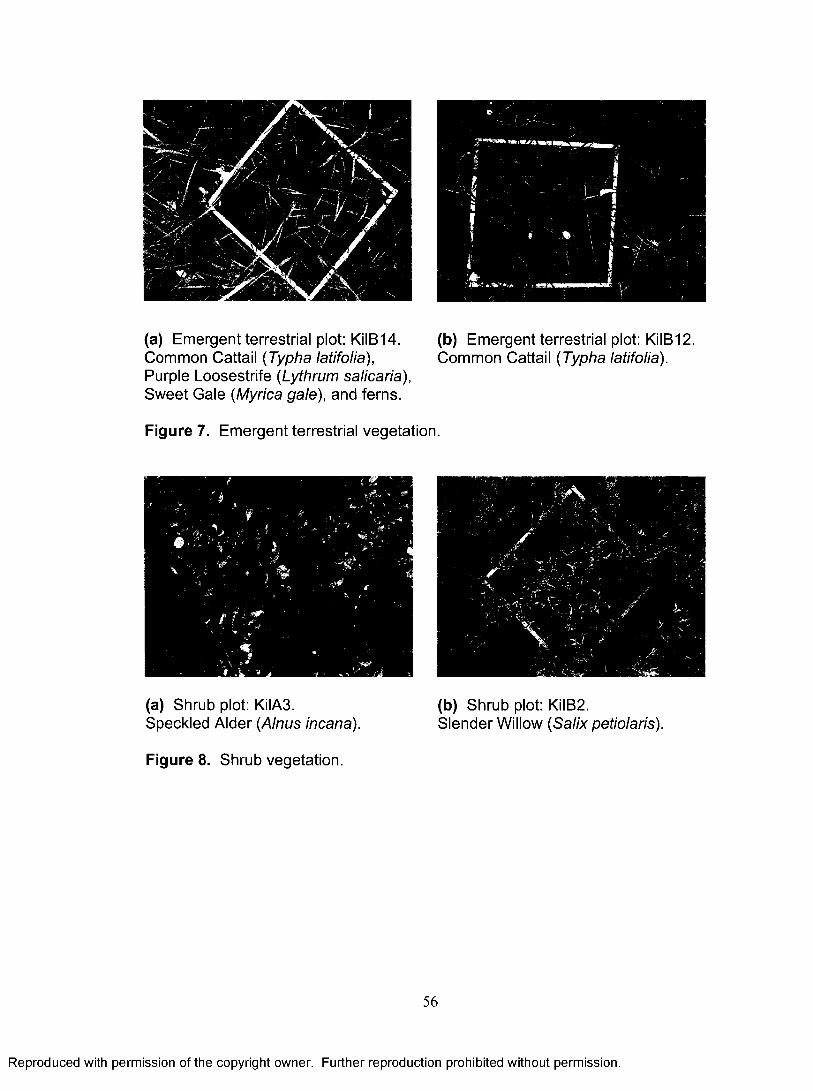
(a) Emergent terrestrial plot: KilB 14. (b) Emergent terrestrial plot: KilB12.Common Cattail (Typha latifolia), Common Cattail (Typha latifolia).Purple Loosestrife (Lythrum salicaria),Sweet Gale (Myrica gale), and ferns.

Figure 7. Emergent terrestrial vegetation.

(a) Shrub plot: KilA3.Speckled Alder (Alnus incana).

(b) Shrub plot: KilB2.Slender Willow (Salix petiolaris).

Figure 8. Shrub vegetation.

56


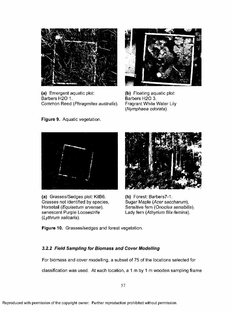
(a) Emergent aquatic plot:Barbers H20 1.Common Reed (Phragmites australis).

Figure 9. Aquatic vegetation.

(a) Grasses/Sedges plot: KilB6. Grasses not identified by species, Horsetail (Equisetum arvense), senescent Purple Loosestrife (Lythrum salicaria).

(b) Floating aquatic plot: Barbers H20 3.Fragrant White Water Lily (Nymphaea odorata).

(b) Forest: Barbers7-1.Sugar Maple (Acer saccharum), Sensitive fern (Onoclea sensibilis), Lady fern (Athyrium filix-femina).

Figure 10. Grasses/sedges and forest vegetation.

3.2.2 Field Sampling for Biomass and Cover Modelling

For biomass and cover modelling, a subset of 75 of the locations selected for

classification was used. At each location, a 1 m by 1 m wooden sampling frame

57


was placed over the vegetation. The plants within the frame were identified,

average height was measured and percent cover was visually estimated. A

digital camera was used to acquire vertically downward colour photographs of

each plot. Figures 11 a and 11 b are examples of photographs acquired during

the field campaign representing terrestrial and aquatic plots.

(a) Terrestrial plot photo: (b) Aquatic plot photo:Kilmarnock B14. Kilmarnock A1.

Figure 11. Terrestrial and Aquatic Field Plots.

Due to inclement weather and the subsequent delay of image acquisition during

the summer of 2003, vegetation was not clipped at this stage, but field plots were

marked for future reference. Following image data acquisition, all above ground

vegetation within the sampling frame was clipped, bagged and transported back

to the lab. The vegetation was stored in a refrigerator at a temperature range of

0-5°C. Plants were chopped and then oven dried at 105°C for 24 hours to

achieve a dry biomass measure in g/m2. Separate measurements were made for

green and senescent (yellow) vegetation. Within the literature (Cole, 1992;

Bartlett and Klemas, 1980; Linthurstand Reimold, 1978; Streever et al., 1998;

58


Hill et al., 1997; Cole et al., 2001) a consistent drying time for wetland plants

could not be found and, as a result, drying curves were assembled for each

vegetation type collected to support the drying time of 24 hours. Figures 12 and

13 show drying curves assembled for floating aquatic and emergent terrestrial

vegetation, respectively, where vegetation was weighed hourly for a period of

more than 24 hours. The weight curve shown in Figure 12 begins levelling off

around 12 hours, while Figure 13 shows some slight variation in weight between

12 -23 hours.

Drying Curve for Water Lily Barbers H20 Plot #5 Live Green Biomass

800

700

600

o>400

O)

300

200

100

1 2 3 4 5 6 7 8 9 10 11 12 13 14 15 16 17 18 19 20 21 22 23 24 25 26 27 28 29 30 31 32 33 34

Time (hours)

Figure 12. Drying Curve for green floating aquatic vegetation.

59


Drying Curve for Live Cattail Kilmarnock-A Plot #2 Live Green Biomass

1400

1200

1000

3 800

U)

600

400

200

1 2 3 4 5 6 7 8 9 10 11 12 13 14 15 16 17 18 19 20 21 22 23 24 25

Time (hours)

Figure 13. Drying curve for green emergent terrestrial vegetation.

3.3 Ikonos Data Acquisition

Ikonos was used as the image source due to its high resolution capabilities with a

nominal ground pixel size of 0.82 metres for panchromatic and 3.2 metres for

multispectral at nadir viewing. The satellite also has off-nadir viewing capabilities

acquiring 1 metre pixel spacing for panchromatic and 4 metres for multispectral

channels. Ikonos has an image swath width of 11.3 kilometers at nadir and 13.8

kilometers at 26 degrees off-nadir. The revisit rate of the satellite is between 2-3

days, allowing for the frequent acquisition of imagery for a particular point on the

Earth.

60


Ikonos multispectral and panchromatic cloud free imagery was acquired on

August 25th, 2003. Due to persistent cloud cover prior to this date, imagery was

not acquired earlier in the season. Peak productivity, however, occurred in

August of 2003 so this late acquisition date was not a constraint. Peak

productivity was essential for this study because biological features such as plant

productivity and biodiversity can be inferred from full growth vegetation and

vegetation communities are more easily identifiable from full-growth imagery

(Arzandeh and Wang, 2003). Field work was conducted in the 6 weeks before

and 2 weeks after image acquisition to ensure that the reference data accurately

depicted ground conditions at the time of scene acquisition. Vegetation

measurement and biomass sampling was conducted as close to image

acquisition (within 2 weeks).

3.4 Image Georeferencing

The image provider (Space Imaging) performed a standard geometric correction

of the raw image data and re-sampled the image to the Universal Transverse

Mercator (UTM) (zone 18, datum NAD 83) projection using cubic convolution

interpolation.

The multispectral and panchromatic imagery were georeferenced more precisely

using 17 ground control points at intersecting roadways and other landmark

features, whose positions were measured using differential GPS. A first order

polynomial affine transformation and nearest neighbour resampling were used,

61


with Root mean square (RMS) errors of (0.05 (x), 0.05 (y)} and {0.14 (x), 0.13(y)}

pixels for the multispectral and panchromatic images, respectively.

3.5 Image Data Transformations

A mask of the three wetland areas used in this study was manually delineated

and various data types were derived from the multispectral imagery including:

vegetation indices, texture measures and principal components.

3.5.1 Vegetation Indices

Due to the limited spectral information available from Ikonos data, only

vegetation indices that use the visible or near infrared bands were applied in this

research. Vegetation indices were derived as described in Chapter 2 and

included: ASVI, DVI, MSAVI, NDVI, RVI, SAVI and TVI (as defined in Chapter 2

and Bannari et al., 1995; Eastwood et al., 1997; Ozesmi et al., 2002; TAN et al.,

2003). Some of these are ‘soil-adjusted’ indices that were selected because the

marshes included significant amounts of yellow senescent vegetation and small

amounts of bare ground visible from above that were assumed to affect the

green vegetation reflectance signal.

3.5.2 Texture Analysis

Eight co-occurrence texture measures Homogeneity (HOM), Contrast (CON),

Dissimilarity (DIS), Mean (MN), Standard Deviation (STDEV), Entropy (ENTR),

62


Angular Second Moment (A2M), and Correlation (COR); and four GLDV

measures Angular Second Moment (GLA2M), Entropy (GLENTR), Mean (GLMN)

and Contrast (GLCON) were extracted from the green and NIR spectral bands

using two window sizes, 3 x 3 and 5x5 . These bands were selected due to their

visibly greater spatial detail and spectral variance between land cover classes as

well as their lower inter-band correlation (r=0.62). The maximum window size of

5 x 5 was selected because larger windows may have included image data from

other vegetation types or structures.

3.5.3 Principal Component Analysis

Table 1 shows the inter-band correlations, with high correlations (r>0.8) between

all visible bands. The near IR band was not highly correlated with any of the

visible bands.

Table 1. Correlation matrix (showing rvalues) for Ikonos spectral bands.Blue Green Red NearIR

Blue 1.00 0.94 0.96 0.52Green 0.94 1.00 0.95 0.62Red 0.96 0.95 1.00 0.57NearIR 0.52 0.62 0.57 1.00

Principal Component Analysis (PCA) was conducted to provide orthogonal

variables as inputs to the maximum likelihood classifier and to possibly reduce

the number of input variables by using only those PCs that together accounted

for over 95% of the total data variance. Using the spectral bands as input, an

unstandardized PCA was run on the wetland mask. In unstandardized PCA, the

spectral bands with higher variance dominate. Standardized PCA, which does

63


not depend on individual band variance was not available in the PCI software

that was used for all the image processing and analysis. The PCs generated

from the spectral bands were used in classification with the addition of texture

measures (as described below).

After texture measures and vegetation indices were derived another PCA was

run on the wetland mask using all image spectral and texture variables as inputs.

The principal components accounting for >95% cumulative variance were used

as independent variables in stepwise multiple regression analysis for biomass

modelling.

3.6 Wetland Vegetation Classification

An important preliminary step for classification is to determine the image dataset

to use as input to the classifier. For this research, when the image dataset was

complete, training data were generated for the 3 x 3 pixel window at each

location where the vegetation had been identified in the field. Single pixel

training data were not used as there were not enough samples for some classes.

3.6.1 Separability Analysis

Separability analysis was performed using the Bhattacharrya Distance (BD), a

distance measure that accounts for class variance-covariance in calculating the

statistical separation between pairs of sample training data distributions (Haralick

and Fu, 1983; Jensen, 1996).

64


In the PCI algorithm, BD is scaled to a range of 0 - 2, where 0 represents

complete overlap between training class distributions and 2 indicates complete

separation between classes.

For this research, separability analysis was initially conducted using all training

data for seven wetland classes to determine which combination of input variables

had the best potential to distinguish between the seven classes. First, each

texture measure was combined with the four spectral bands in individual

separability analyses. The textures that increased the minimum and average

class BD the most were then tested with different spectral datasets including the

raw bands, vegetation indices and principal components. Once the best data

combinations were determined, separability analysis was conducted again for

varying wetland class combinations, which were based on class pairs showing

the lowest separability. The goal was to determine the best input variable

combination that included variables not highly correlated with each other (r <

0.8). These final variables were used as inputs to several classification tests of

varied land cover classes as described below.

3.6.2 Maximum Likelihood Classification

For classification, the field and image data were randomly divided into equal

training and validation datasets. Maximum likelihood classification was

conducted using probability density function bounds of three standard deviations

for the training data distributions and equal a priori probabilities for all classes.

65


Bounds of three standard deviations were used because each training site had

been field verified and there was high certainty that all pixels in each training

sample represented the assigned class. Equal a priori probabilities were used

because it could not be determined before classification what the class spatial

proportions were. Classifications were conducted first for seven wetland classes:

Emergent Terrestrial (EM), Shrubs (SHR), Emergent Aquatic (EMAQ), Floating

Aquatic (FLAQ), Grasses/Sedges (GS), Forest (FOR) and Open Water (OW). To

improve classification accuracy, the EM and SFIR classes were merged and

classification was repeated for six classes. Further merging was done to create

a Terrestrial Marsh (TERm) class, which was composed of EM, SFIR and GS,

and resulted in a final 5 class classification.

3.6.3 Neural Network Classification

Neural network classification was conducted as it is not constrained by the

number of input variables or normal data distribution requirements. A multilayer

feed forward back-propagating neural network was used to classify the wetland

areas. The neural networks were trained using the 5 wetland classes, mentioned

previously, and were run on the wetland mask only. Several tests were

performed changing the configuration of the networks such as the number of

iterations, as well as the momentum and learning rates to achieve convergence

towards the acceptable limits for maximum individual and total errors. PCI

(2004) suggests that a smaller learning rate (0.1) reduces the risk of oscillation

and non-convergence of the training data. A learning rate of 0.1 and a

66


momentum rate of 0.9 were used by Foody et al. (1996) and Pierce et al. (1994).

Kavzoglu and Mather (2003) found that a learning rate of 0.1 or 0.2 with a

momentum rate of 0.5 or 0.6 resulted in higher classification accuracy. The

number of iterations was increased from 1,000 to 100,000 to obtain convergence

of the training data, though the lowest achieved maximum individual error (1.43)

still exceeded the limit of 0.001. Spectral and textural data producing the best

results for the ML classification were used as inputs for the neural networks

though, for some configurations, vegetation indices were included as inputs to

determine if they produced higher classification accuracies. The 4th network

used the momentum and learning rates proposed by Kavzoglu and Mather

(2003), though maximum individual and total errors still exceeded the limits. The

number of samples was derived from a random 50% selection of the 107 training

plots used for classification, each consisting of 3 x 3 pixels. Table 2 shows the

configuration of all neural networks run for this analysis.

67


Table 2. Neural network configurations.Neural

NetworkNumber

Inputs MomentumRate

LearningRate

MaximumIterations

1 Spectral bands plus A2M5grn and CON5nir

0.9 0.1 1,000

2 PC1-4 (derived from spec bands) plus

A2M5grn and CON5nir

0.9 0.1 1,000

3 Spectral bands, A2M5grn and CON5nir

plus MSAVI, NDVI, RVI, SAVI and TVI

0.9 0.1 1,000



0.6 0.2 1,000


0.9 0.9 1,000


0.9 0.1 25,000


0.9 0.1 100,000


0.9 0.1 100,000


0.9 0.1 250,000

10 PC1 and PC2 (derived from spec bands using

entire image) plus GRN5TEX

0.9 0.1 100,000


entire image) plus NIR5 TEX

0.9 0.1 100,000


wetland mask) plus GRN5 TEX

0.9 0.1 100,000


wetland mask) plus NIR5 TEX

0.9 0.1 100,000



0.9 0.1 100,000

All maps produced by the classifications above were mode filtered to reduce

noise.

68


3.6.4 Classification Accuracy Assessment

Accuracy was assessed using a standard error matrix and Khat statistic as

described in Chapter 2. Due to small numbers of sample sites for some classes,

3 x 3 validation windows were used. The pixels within each 3x3 window were

obviously highly autocorrelated (adjacent pixels are more likely similar classes

than dissimilar classes), but it was not feasible to visit enough individual sample

pixel locations to develop a validation dataset of low spatial autocorrelation.


All the image variables listed above were extracted for the single pixel at each

biomass field plot location. Forward stepwise regression of these image

variables against dry biomass and cover was conducted. Probabilities to enter

and remove were set at 0.05 and 0.10, respectively. Scatterplots were analysed

to evaluate linearity, which showed nonlinear relationships between many of the

independent image variables and the dependent biomass and cover variables.

As a result, log transformation of biomass and cover values were deemed

appropriate. Multicollinearity was reduced by using only image variables that

were not highly correlated with each other as inputs (r < 0.80) and where the

variance inflation factor (VIF) for each independent variable fell within the desired

limit (Allison, 1999; Freund and Wilson, 1998).

69


For biomass, seven variations of regressions were conducted that represented

combinations of green and senescent vegetation for the terrestrial and aquatic

environments, as shown in Table 3.

Table 3. Variations for biomass regression analysis.Terrestrial and Aquatic

PlotsTerrestrial Plots Aquatic Plots

Green and Senescent biomass combined

Green and Senescent biomass combined Green biomass

Green biomass Green biomassSenescent biomass Senescent biomass

Vegetation cover modelling was conducted only for aquatic plots, as cover was

too difficult to reliably estimate for the terrestrial plots where vegetation was often

vertically bent into the plot from outside or out of the plot from inside. The visual

field estimates of cover were used as well as cover estimates derived from

maximum likelihood classification of a vertically downward photograph taken at

each biomass field plot. The maximum likelihood classifier produced a map for

each photo of live vegetation, senescent vegetation, and open water. This

process was conducted for all aquatic plots, though it worked best for floating

vegetation which was least influenced by shadow and vegetation overlay due to

wind.

The two estimates of percent cover were also used as independent variables

against dry biomass to determine if percent cover was an indicator of biomass.

70


3.7.1 Biomass Model Assessment and Validation

Model performance was evaluated based on the adjusted coefficient of

determination ( / ^ ) for the model and the R2 change produced by each variable;

the Se and p values; and the number of variables entered into the model based

on the 1:10 variable to sample ratio rule (Stevens, 1996). Model residuals were

checked for uniformity and normality. The Variance inflation factor (VIF) was

also calculated for each model as VIF = ̂ (Freund and Wilson, 1998). It

indicates multicollinearity within the model when VIF values exceed the

calculated threshold VIF.

For the best model, five separate validation runs of randomly splitting the data

into 70% training and 30% validation were conducted. Errors were compared for

a one variable model (since the MN5grn variable dominated all models) and

models with all significant variables entered. Following this, R2, Se, mean error,

mean absolute error, and RMSE were calculated and averaged for the five

validations. The latter three values were used to assess model prediction error

and were also expressed as percentages of the mean field measured biomass

values for each given dataset.

71


Chapter Four: Results

4.1 Principal Component Analysis

PCA conducted using the four spectral bands for the wetland mask area showed

that PC1 accounted for 95.81% of the variance and had a perfect inverse

correlation with the NIR band, where darker brightness indicated increased NIR

reflectance. From Table 4, the green band had the next highest correlation

(r = -0.64) with PC1 indicating that PC1 represents a vegetation gradient. PC2

accounted for 4.01% of the variance and was highly correlated with the visible

bands (r > 0.75) showing an increased brightness with visible band reflectance.

Roads and bare soil had the highest brightness and vegetation had a mixture of

grey tones, which could indicate that PC2 was a moisture gradient for land

features only. Some agriculture fields, however, appeared darker than open

water which would suggest that PC2 was not a true moisture gradient. PC2 was

therefore most likely a vegetation gradient highly correlated with the visible range

of the spectrum. PC3 and PC4 accounted for 0.15% and 0.03% of the variance

respectively, though they were retained for use in further analysis as low

variance PCs can contribute information in a certain area of the image or at

specific locations such as edges.

Table 4. PCA of spectral data: Factor loadings table.Correlations shown as rvalues.

PC1 PC2 PC3 PC4Blue -0.55 0.80 -0.07 -0.24Green -0.64 0.75 0.14 0.01Red -0.60 0.78 -0.17 0.03NIR -1.00 -0.03 0.00 0.00

72


PCA conducted using all image spectral and texture variables also produced 2

significant components where PC1 and PC2 accounted for 96.84% and 3.02% of

the variance respectively. This is because unstandardized PCA using the

variance-covariance matrix is dominated by high variance variables. The

textures varied only within a mean range of 0.07-6.3DN, with the MN5nir texture

variable contributing the most, though it was found to be highly correlated with

the NIR band (r=0.93). The mean DN values for the visible bands ranged from

167.68-272.10 with the NIR band showing the highest mean of 549.46DN.

Consequently, the NIR band also dominated PC1 and the visible bands

dominated PC2 as above. It was concluded that unstandardized PCA with

spectral plus low variance textures does not produce PCs showing textural

information, but rather is dominated by spectral information. Achieving PCs

representing spectral and texture variables together was not possible without

standardizing all input bands or exporting all the data and conducting

standardized PCA in another software package. Neither of these was attempted

due to the large amount of additional processing and analysis that would be

required. Instead, in wetland classification and biomass modelling input

variables were used that were not highly correlated with each other (r < 0.8).

4.2 Separability Analysis

Separability analysis was used, as described in section 3.6.1, to determine the

best combination of image data, including spectral bands, principal components,

73


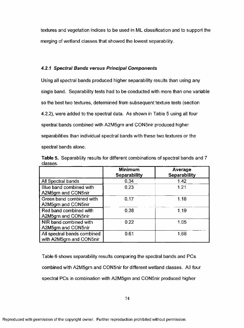
textures and vegetation indices to be used in ML classification and to support the

merging of wetland classes that showed the lowest separability.

4.2.1 Spectral Bands versus Principal Components

Using all spectral bands produced higher separability results than using any

single band. Separability tests had to be conducted with more than one variable

so the best two textures, determined from subsequent texture tests (section

4.2.2), were added to the spectral data. As shown in Table 5 using all four

spectral bands combined with A2M5grn and CON5nir produced higher

separabilities than individual spectral bands with these two textures or the

spectral bands alone.

Table 5. Separability results for different combinations of spectral bands and 7 classes.

MinimumSeparability

AverageSeparability

All Spectral bands 0.34 1.42Blue band combined with A2M5grn and CON5nir

0.23 1.21

Green band combined with A2M5grn and CON5nir

0.17 1.18

Red band combined with A2M5grn and CON5nir

0.38 1.19

NIR band combined with A2M5grn and CON5nir

0.22 1.05

All spectral bands combined with A2M5grn and CON5nir

0.61 1.68

Table 6 shows separability results comparing the spectral bands and PCs

combined with A2M5grn and CON5nir for different wetland classes. All four

spectral PCs in combination with A2M5grn and CON5nir produced higher

74


separabilities than using only PC1 and PC2 with these textures, so all four PCs

were retained for classification. The spectral band combination and PC 1-4

combination had similar if not identical results for all wetland class combinations.

Table 6. Separability results for spectral bands and PCs combined with A2M5grn and CON5nir with varying number of wetland classes._______

Number of Wetland Classes

MinimumSeparability

AverageSeparability

Class Pair with Minimum

SeparabilitySpectralbandscombinedwithA2M5grnandCON5nir

7 classes ALL TRN

0.61 1.68 SHR and OW

6 classes with EM and SHR

merged

1.22 1.87 EM/SHR merged and GS

6 class with SHR and GS

merged

0.49 1.82 EM and SHR/GS merged

5 class with EM, EMAQ and

GS merged

0.45 1.81 EM/EMAQ/GS merged and SHR

5 class with EM, SHR and GS merged

1.63 1.91 TERm and EMAQ

PC1-PC4combinedwithA2M5grnandCON5nir

7 classes ALL TRN

0.61 1.70 EM and SHR

6 classes with EM and SHR

merged

1.21 1.87 EM/SHR merged and GS

6 class with SHR and GS

merged

0.49 1.82 EM and SHR/GS merged

5 class with EM, EMAQ and

GS merged

0.45 1.81 EM/EMAQ/GS merged and SHR

5 class with EM, SHR and GS merged


75


4.2.2 Determining the Best Texture Variables for Classification

Table 7 shows the separability results comparing a small subset of 3 x 3 and 5 x

5 textures. In general, separability was higher for textures using a 5 x 5 window

size compared to a 3 x 3 window size, with the exception of MN3nir discussed

later. As a result 3 x 3 textures were discarded from further classification

analysis.

Table 7. Separability results for selected 3 x 3 and 5 x 5 textures based on 7 classes.

Minimum Separability AverageSeparability

3 x 3 5 x 5 3 x 3 5 x 5Spectral bands + HOM-grn

0.47 0.54 1.47 1.49

Spectral bands + HOM-nir

0.49 0.51 1.46 1.48

Spectral bands + STDEV-grn

0.42 0.45 1.49 1.51

Spectral bands + STDEV-nir

0.45 0.50 1.48 1.49

Table 8 shows the 5 highest ranked textures each combined with the spectral

bands. MN5nir ranked first due to this texture showing the highest minimum

separability, followed by A2M5grn, CON5nir, A2M5nir, and MN3nir. MN5nir and

MN3nir were, however, not used in ML classification because they were highly

correlated to each other (r=0.99), to NIR (r=0.94 and r=0.96, respectively) and to

PC1 (r=-0.93 and r=-0.96, respectively).

76


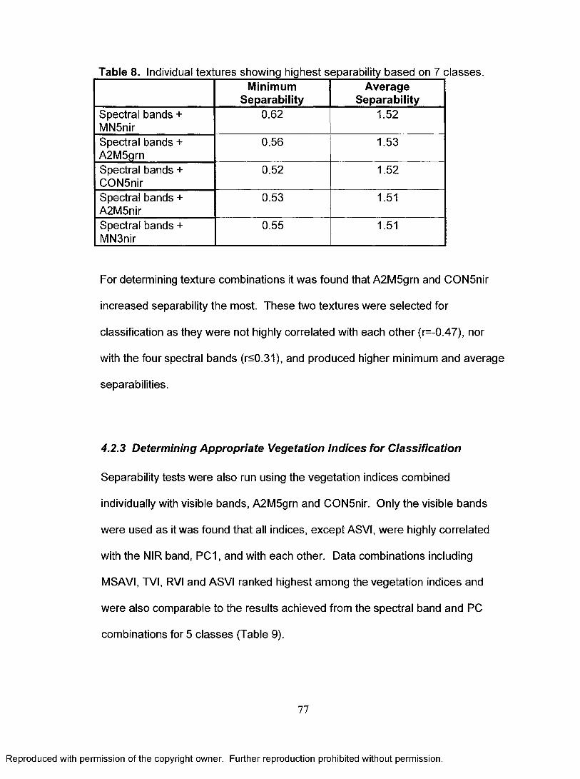
Table 8. Individual textures showing highest separability based on 7 classes.Minimum

SeparabilityAverage

SeparabilitySpectral bands + MN5nir

0.62 1.52

Spectral bands + A2M5grn

0.56 1.53

Spectral bands + CON5nir

0.52 1.52

Spectral bands + A2M5nir

0.53 1.51

Spectral bands + MN3nir

0.55 1.51

For determining texture combinations it was found that A2M5grn and CON5nir

increased separability the most. These two textures were selected for

classification as they were not highly correlated with each other (r=-0.47), nor

with the four spectral bands (r<0.31), and produced higher minimum and average

separabilities.

4.2.3 Determining Appropriate Vegetation Indices for Classification

Separability tests were also run using the vegetation indices combined

individually with visible bands, A2M5grn and CON5nir. Only the visible bands

were used as it was found that all indices, except ASVI, were highly correlated

with the NIR band, PC1, and with each other. Data combinations including

MSAVI, TVI, RVI and ASVI ranked highest among the vegetation indices and

were also comparable to the results achieved from the spectral band and PC

combinations for 5 classes (Table 9).

77


4.2.4 Merging Wetland Classes based on Separability

Separability analysis was initially performed using seven wetland classes (EM,

SHR, FLAQ, EMAQ, OW, FOR and GS), though this produced the lowest

average and minimum separabilities (Tables 6 and 9). Class pairs showing

minimum separability were combined, including EM with SHR and SHR with GS.

Further testing of these two 6 class sets, showed that the merging of EM and

SHR resulted in higher minimum and average separabilities, while the merging of

SHR and GS produced lower separabilities and therefore this combination was

not used for further classification analysis. Despite the overall increased

separability for 6 classes it was felt that further merging was necessary as some

wetland classes, such as GS and EMAQ, had small sample sizes or were difficult

to spectrally distinguish. Different merging tests were performed to determine

the best combination of five wetland classes. Looking at the class photos

(examples given in chapter 3), it appears that EM, EMAQ and GS would be

spectrally similar and therefore should be merged. This combination, however,

produced the lowest minimum separability, as seen in Table 6. The best

combination for 5 classes consisted of Terrestrial marsh (EM, SHR and GS

combined), FLAQ, EMAQ, OW and FOR. These classes do not correspond

exactly to those of the Ontario Wetland Evaluation System but they are the

classes that are separable using Ikonos spectral and textural information.

Table 9 shows the separability results for the top three data combinations for

varying number of wetland classes, showing a dominance of vegetation indices,

78


particularly MSAVI for all class combinations. For 5 classes the PC 1-4 and

spectral band combinations tied for first, followed by the ASVI combination, and

tied for third were the RVI and MSAVI combinations.

Table 9. Separability results for top three data combinations for 7, 6 and 5 wetland classes based on 50% training 3x3 clusters.__________________

Wetland Classes Used

During Classification

MinimumSeparability

AverageSeparability

Class Pair with

Minimum Separability

MSAVIcombination*

7 classes

0.56 1.79 EM and SHR

RVIcombination 0.55 1.79 EM and SHR

TVIcombination 0.54 1.79 EM and SHR

ASVIcombination 6 classes

(EM and SHR merged)

1.46 1.87 EM/SHR and FLAQ

MSAVIcombination 1.43 1.87 EM/SHR and

GSTVIcombination 1.42 1.87 EM/SHR and

FLAQPC1-4,A2M5grn and CON5nir

5 classes (EM, SHR, GS

merged)


Spectral bands, A2M5grn and CON5nir


ASVIcombination 1.46 1.88 TERm and

FLAQRVIcombination 1.43 1.89 TERm and

FLAQMSAVIcombination 1.43 1.88 TERm and

FLAQ‘ Combination denotes that each vegetation index was combined with visible bands, A2M5grn and CON5nir.

4.3 Classification Analysis

Results produced from the ML and neural network classifications are presented

and compared in the following sections.


4.3.1 Maximum Likelihood Classification

Classifications results are presented for the top three data combinations derived

from the separability analysis for 7, 6 and 5 classes. The error matrices and

classified maps are presented only for those classifications with the highest

overall accuracy in each class combination.

4.3.1.1 Classification using Seven Classes

Based on the separability analysis for 7 classes, the MSAVI combination ranked

first followed by the RVI and TVI combinations, respectively. The error matrix

and the classified map for the MSAVI classification are shown below.

1) MSAVI Combination

The overall classification accuracy for the 7 class MSAVI combination was 61.3%

and the computed Khat statistic was 0.47.

Table 10. Error matrix for 7 class MSAVI classification.Rows contain number of pixels assigned as reference data and columns contain

EM SHR FLAQ EMAQ OW FOR GS Row TotalEM 155 21 6 16 0 0 0 198SHR 30 51 0 23 0 8 5 117FLAQ 0 0 36 0 0 0 0 36EMAQ 7 8 0 0 0 0 3 18OW 0 0 0 0 45 0 0 45FOR 0 23 0 0 0 0 4 27GS 25 0 2 0 0 0 0 27ColumnTotal 217 103 44 39 45 8 12 468

80


Table 10 shows the error matrix for the 7 class MSAVI classification. Errors of

omission (across the table rows) for the emergent terrestrial class occurred in

misclassification predominantly as shrub and emergent aquatic, as well as lesser

confusion with floating aquatic. Errors of commission (down the table columns)

for emergent terrestrial occurred when shrub and grasses/sedges were

incorrectly classified as emergent terrestrial. Shrub class errors of omission

occurred in misclassification predominantly as emergent terrestrial and emergent

aquatic. Errors of commission resulted when forest and emergent terrestrial

were incorrectly classified as shrubs. Floating aquatic was well classified,

although small errors of commission occurred with emergent terrestrial and

grasses/sedges. Emergent aquatic was completely misclassified predominantly

as shrubs and emergent terrestrial, while open water was classified correctly with

no errors of omission or commission. Forest was entirely misclassified showing

errors of omission and commission predominantly with shrubs. Grasses/sedges

were also completely misclassified showing errors of omission as

grasses/sedges were confused with emergent terrestrial and floating aquatic.

Errors of commission occurred when shrub, forest and emergent aquatic were

incorrectly classified as grasses/sedges.

The producer and user accuracies for the 7 class MSAVI combination are given

in Table 11 with the resulting map shown in Figure 14. If all classes are

considered equally important, the average producer and user accuracies are only

43.3% and 46.0%.

81


Table 11. Producer and user accuracies for 7 class MSAVI classification.Producer’s Accuracy (%) User’s Accuracy (%)

Emergent Terrestrial 71.4 78.3Shrubs 49.5 43.6Floating Aquatics 81.8 100.0Emergent Aquatic 0.0 0.0Open Water 100.0 100.0Forest 0.0 0.0Grasses/Sedges 0.0 0.0

From visual assessment of Figure 14 it appears that the emergent aquatic class,

shown in red, is generally located in areas where emergent terrestrial and shrub

vegetation, shown in brown and pink, were observed in the field. Emergent

aquatic vegetation should occur in closer proximity to areas of open water and

floating aquatic vegetation, as was seen in the field.

Figure 14. MSAVI classification for 7 classes with mode filter applied.

82


2) RVI Combination

The RVI combination achieved an overall classification accuracy of 61.1% and a

Khat statistic of 0.46. The patterns of confusion between classes mirrored those

of the MSAVI classification.

3) TVI Combination

An overall accuracy of 60.3% with a Khat statistic of 0.45 was achieved for the 7

class TVI classification. The significant difference for the TVI classification

compared to the other 7 class combinations was that open water was confused

with shrubs, which resulted in lower user accuracy for this class. All other class

confusions, stated previously, also existed for the TVI classification.

From all classifications using 7 classes, shrubs, emergent aquatic and

grasses/sedges were consistently confused with emergent terrestrial vegetation,

which results from a spatial dominance of the emergent terrestrial class,

particularly Common cattail (Typha latifolia), while shrubs, emergent aquatic and

grasses/sedges were much less common.

4.3.1.2 Classification using Six Classes

From the separability analysis for six classes, with emergent terrestrial and

shrubs merged, the ASVI, MSAVI and TVI combinations ranked first through

third, respectively. The highest overall classification accuracy was, however,

achieved from the TVI combination which will be discussed first and in the most

83


detail, followed by MSAVI and lastly by ASVI which achieved the lowest overall

classification accuracy.

1) TVI Combination

The TVI combination achieved an overall accuracy of 71.6% and a Khat statistic

of 0.44. The large difference between the overall accuracy and the Khat statistic

exists because the overall accuracy is affected by unequal sample sizes between

classes, where emergent terrestrial/shrub has the largest number of reference

pixels and is also well classified. The Khat statistic is, however, not affected by

this. If class sample sizes reflect the actual aerial proportions, then overall

accuracy is a good indicator of map accuracy.

Table 12. Error matrix for 6 class TVI classification.Rows contain number of pixels assigned as reference data and columns contain

EM/SHR FLAQ EMAQ OW FOR GS Row TotalEM/SHR 262 6 37 0 7 3 315FLAQ 0 36 0 0 0 0 36EMAQ 16 0 0 0 0 2 18OW 8 0 0 37 0 0 45FOR 21 0 1 0 0 5 27GS 23 4 0 0 0 0 27ColumnTotal 330 46 38 37 7 10 468

Table 12 shows the error matrix for the 6 class TVI classification.

Errors of omission for the combined emergent terrestrial/shrub class occurred in

misclassification with all classes, except open water, particularly as emergent

aquatic. Errors of commission for emergent terrestrial/shrub occurred when

grasses/sedges, forest, emergent aquatic and open water were incorrectly

84


classified as emergent terrestrial/shrub. Errors of commission for floating aquatic

occurred when emergent terrestrial/shrub was incorrectly classified as floating

aquatic. Errors of omission for the emergent aquatic class occurred in

misclassification as predominantly emergent terrestrial/shrub, as well as lesser

confusion with grasses/sedges. Errors of commission for emergent aquatic

occurred when predominantly emergent terrestrial/shrub was incorrectly

classified as emergent aquatic. Open water was well classified, although it was

confused with emergent terrestrial/shrub resulting in a lower user accuracy.

Forest was entirely misclassified showing errors of omission and commission

with emergent terrestrial/shrub. Grasses/sedges were also completely

misclassified showing errors of omission with emergent terrestrial/shrub, as well

as lesser confusion with floating aquatic. Errors of commission occurred when

forest, emergent terrestrial/shrub and emergent aquatic were incorrectly

classified as grasses/sedges.

Based on Table 13 the average producer and user accuracies for the 6 class TVI

classification are 42.9% and 44.2%.

Table 13. Producer and user accuracies for 6 class TVI classification.Rows contain reference cata and columns contain classified data.

Producer’s Accuracy (%) User’s Accuracy (%)Emergent Terrestrial/ Shrub

79.4 83.2

Floating Aquatic 78.3 100.0Emergent Aquatic 0.0 0.0Open Water 100.0 82.2Forest 0.0 0.0Grasses/Sedges 0.0 0.0

85


From Figure 15 the emergent aquatic class, shown in red was again found in

areas where emergent terrestrial and shrub vegetation, shown in brown, were

seen in the field.

Figure 15. TVI classification for 6 classes with mode filter applied.

2) MSAVI Combination

For the MSAVI combination an overall accuracy of 71.2% and a Khat statistic of

0.45 were achieved, with similar patterns of class confusion as the MSAVI

classification.

3) ASVI Combination

An overall accuracy of 69.9% and a Khat statistic of 0.42 were achieved for the

ASVI classification. The significant difference for the ASVI classification

86


compared to the other 6 class combinations was that some forest pixels were

correctly classified resulting in higher producer and user accuracies for this class.

Another significant difference was that errors of commission occurred when

floating aquatic was incorrectly classified as emergent terrestrial/shrub.

From all classifications using six classes, emergent aquatic was consistently

confused with combined emergent terrestrial/shrub and grasses/sedges. Forest

was also consistently confused with combined emergent terrestrial/shrub.

4.3.1.3 Classification using Five Classes

Based on the 5 class separability analysis with emergent terrestrial, shrubs and

grasses/sedges merged, the following combinations ranked from first to third: the

PC 1-4 and spectral band combinations tied for first, followed by the ASVI

combination, and tied for third were the RVI and MSAVI combinations. The

highest overall classification accuracy resulted from the spectral band, A2M5grn

and CON5nir combination, which will be discussed first and in the most detail.

1a) Spectral bands, A2M5grn and CON5nir Combination

An overall accuracy of 84.8% and a Khat statistic of 0.66 were achieved for the

spectral bands, A2M5grn and CON5nir combination.

87


Table 14. Error matrix for 5 class Spectral bands, A2M5grn and C0N5nir classification.Rows contain number of pixels assigned as reference data and columns contain number of pixels assigned as classified data._____________________________

TERm FLAQ EMAQ OW FOR Row TotalTERm 309 18 0 1 14 342FLAQ 2 34 0 0 0 36EMAQ 16 2 0 0 0 18OW 0 0 0 45 0 45FOR 18 0 0 0 9 27ColumnTotal 345 54 0 46 23 468

Table 14 shows the error matrix for the 5 class spectral band, A2M5grn and

CON5nir classification. Errors of omission for the terrestrial marsh class

occurred in misclassification as floating aquatic and forest. Dominant errors of

commission for terrestrial marsh occurred when forest and emergent aquatic

were incorrectly classified as terrestrial marsh. Errors of commission for floating

aquatic occurred as terrestrial marsh was incorrectly classified as floating

aquatic. Errors of omission for the emergent aquatic class occurred in

misclassification as predominantly terrestrial marsh, as well as lesser confusion

with floating aquatic. In general, open water was very well classified. Forest had

low producer and user accuracy due to confusion of forest with terrestrial marsh.

From Table 15 the average producer and user accuracies for the 5 class spectral

band, A2M5grn and CON5nir classification are 63.6% and 57.9%.

88


Table 15. Producer and user accuracies for 5 class spectral bands, A2M5grn and CON5nir classification.

Producer’s Accuracy (%) User’s Accuracy (%)Terrestrial Marsh 89.6 90.4Floating Aquatic 63.0 94.4Emergent Aquatic 0.0 0.0Open Water 97.8 100.0Forest 39.1 33.3

Figure 16. Spectral band classification for 5 classes with mode filter applied.

Even though none of the validation samples for the emergent aquatics were

classified correctly (Tables 14 and 15), the locations of the pixels assigned to this

class, shown in red in Figure 16, correspond well with the locations in which this

vegetation class was observed in the field. In addition, the largest percentage of

emergent aquatic vegetation, dominated by Common Reed (Phragmites

89


australis), that was found during the field campaign occurred in Kilmarnock

marsh and was either dense cover or interspersed with open water, as shown in

Figures 17a and 17b. Field samples were predominantly taken from areas of

dense emergent aquatic vegetation to minimize the confusion between floating

aquatic and emergent aquatic vegetation. This type of dense aquatic cover

corresponds to the area in Figure 16 which was classified as emergent aquatic.

From Figure 16 the largest visual representation of the emergent aquatics class

is found in Kilmarnock marsh and secondly in a finger of Barbers creek marsh.

(a) Emergent aquatic vegetation (b) Dense emergent aquatic vegetation interspersed with open water in identified in Kilmarnock marsh AugustKilmarnock marsh August 2003. 2003.

Figure 17. Emergent aquatic vegetation.

1b) PC1-4, A2M5grn and CON5nir Combination

An overall classification accuracy of 83.1% and a Khat statistic of 0.63 were

achieved for the PC1-4, A2M5grn and CON5nir combination. The significant

difference for the PC1-4 combination, compared to the spectral band

combination, was that terrestrial marsh was incorrectly classified as emergent

aquatic, resulting in lower producer accuracy.

90


2) RVI Combination and MSAVI combination

For the RVI and MSAVI combinations overall accuracies of 78.4% and 77.6%,

and Khat statistics of 0.53 and 0.52 were achieved, respectively. For both the

RVI and MSAVI combinations the most significant difference compared to the

other 5 class combinations was the complete misclassification of forest as

terrestrial marsh. Another difference was that these combinations attained the

highest producer and user accuracies for floating aquatic.

3) ASVI Combination

The ASVI combination resulted in an overall classification accuracy of 75.0% and

a Khat statistic of 0.46. Compared to the other 5 class combinations the most

significant difference for the ASVI classification was the lower producer and user

accuracies for forest and floating aquatic. In general, there was significant

confusion discriminating between forest and terrestrial marsh, and floating

aquatic and terrestrial marsh.

From all classifications using 5 classes, emergent aquatic and forest were

consistently confused with terrestrial marsh.

4.3.2 Summary of Classification Results

From assessment of all of the error matrices for the 7, 6 and 5 classes, the

emergent aquatic class was consistently confused with terrestrial marsh

vegetation, which included emergent terrestrial, shrubs and grasses/sedges.

91


The predominant misclassification of emergent aquatic as terrestrial marsh for all

classifications can be explained by the structural and subsequent spectral

similarities between Common reed (Phragmites australis) and Common cattail

(Typha latifolia) both dominant vegetation covers in each class respectively.

From Figures 18a and 18b both vegetation species have similar flat leaf structure

and form large dense colonies. Common cattail (Typha latifolia) was typically

taller than Common reed (Phragmites australis), though this would have little or

no influence on vegetation reflectance. The predominant difference between the

two species is the environment in which they grow, with Common reed

(Phragmites australis) growing in open water areas compared to Common cattail

(Typha latifolia) growing on densely floating mats more similar to a terrestrial

environment.

92


(a). Common Cattail (Typha latifolia) (b). Common Reed (Phragmites vegetation. australis) vegetation.Figure 18. Emergent terrestrial versus emergent aquatic vegetation.

In addition, as can be seen from Table 16, fewer training and validation samples

existed for emergent aquatic which, besides forest, was the most poorly

represented class due to few areas being found on the ground compared to the

dominance of samples representing terrestrial marsh.

Table 16. Number of pixels per wetland class for 5 classes using approximately 50% training and 50% validation 3 x 3 clusters._________________________

Number of pixels per wetland class for 5 classes using 50%

Training 3 x 3

Number of pixels per wetland class for 5 classes using 50 %

Validation 3 x 3Terrestrial Marsh 351 342Floating Aquatic 45 36Emergent Aquatic 27 18Open Water 54 45Forest 18 27


As expected, the classification results showed that overall accuracy significantly

improved as classes were merged, with the highest accuracy obtained using 5

classes as was also seen from the separability analysis. Higher separability,

however, did not always result in higher overall classification accuracy. For 6

classes, the TVI combination, ranked third by separability, resulted in the highest

overall classification accuracy. For this research, separability provided an ideal

starting method for selecting textures and determining which spectral data

combined with those textures should be used for classification. It also supported

the merging of wetland classes that were found to be either spectrally similar or

that had small sample sizes. It should be noted, however, that the results

produced from separability analysis did not correspond exactly to those for

classification accuracy. Separability analysis can aid in input variable selection

and give a general idea of relative potential for classification accuracy, but it was

not a good indicator of final absolute accuracy.

4.3.3 Additional Maximum Likelihood Classifications

Following the results presented above, additional ML classifications were

conducted using input variable combinations that had not ranked in the top three

from separability analysis, to determine if higher classification accuracies could

be achieved.

Since 5 classes were shown to produce significantly better classification results,

compared to 6 and 7 classes, this class combination was selected for these

94


classification tests. Classifications were run for the following vegetation indices

(DVI, NDVI, SAVI and TVI) individually combined with A2M5grn and CON5nir.

These additional VI classifications showed an improvement in overall accuracy

compared to the ASVI, RVI and MSAVI combinations, identified as the best

combinations using separability analysis. The TVI combination produced the

highest overall classification accuracy of 87.8% and the highest Khat statistic of

0.72. The error matrix, producer and user accuracies and a classified map are

presented below.

Table 17. Error matrix for 5 class TVI classification.Rows contain number of pixels assigned as reference data and columns contain number of pixe s assigned as classified data.


Table 17 shows the error matrix for the 5 class TVI classification. Comparing the

TVI classification to the 5 class spectral band combination, discussed previously,

the significant differences are the higher producer and user accuracies for the

terrestrial marsh and forest classes. The same class confusions, discussed

earlier, also occurred for the TVI classification. Table 18 shows the producer and

user accuracies for the 5 class TVI classification with average producer and user

accuracies of 61.7% and 65.4%.

95


Table 18. Producer and user accuracies for 5 class map derived from TVI classification.


The spatial distribution of the emergent aquatic class, shown in red in Figure 19,

is comparable to that seen in Figure 16 and corresponds well with general

observations from the field.

Figure 19. TVI classification for 5 classes with mode filter applied.

96


4.3.4 Neural Network Classification

Unlike ML classification neural networks are not statistical in nature and can

handle a greater number of input variables as well as correlation between

variables. Through the classification process the best combination of inputs are

generally determined. Due to the extensive scope of this research, neural

network classification was limited and therefore inputs paralleled those used in

the best ML classifications, although a greater number of inputs was used in

several configurations. None of the fourteen neural networks fully converged to

achieve both the maximum allowable individual (0.001) and total (0.01) errors.

As shown in Table 19, neural network 10 was the only one to meet the total error

parameter, though its individual error far exceeded the allowable limit. The

smallest individual error was achieved by network 12 which, even after 100,000

iterations, still did not converge.

97


Table 19. Neural network convergence.Neural

NetworkNumber

Inputs Highest Individual Class Error

Total Error Achieved


2.07 0.14

2 PC 1-4 (derived from spec bands) plus

A2M5grn and CON5nir

2.18 0.12



2.17 0.12



1.91 0.09


2.08 0.23


2.00 0.10


2.06 0.08


1.91 0.07


1.94 0.06


entire image) plus GRN5 TEX

1.63 0.01


entire image) plus NIR5 TEX

1.66 0.03


wetland mask) plus GRN5 TEX

1.43 0.02


wetland mask) plus NIR5 TEX

1.93 0.03

14 Spectral bands, A2M5grn and Cor5nir


1.74 0.05

Overall classification accuracies were generally lower for the neural networks

compared to the ML classifications using the same 5 wetland classes. Neural

98


Network 14 achieved the highest overall accuracy of 84.4% and a Khat statistic of

0.64. Table 20 shows the corresponding error matrix.

Table 20. Error matrix for 5 class neural network (#14) classification.Rows contain number of pixels assigned as reference data and columns contain


In comparison to the best ML 5 class classifications, neural network 14 had

similar class confusions, although the network achieved lower producer and user

accuracies for forest and higher producer accuracy for floating aquatic. From

Table 21 when all classes are considered equally important the average

producer and user accuracies are only 56.1% and 59.4% for neural network 14.

Table 21. Producer and user accuracies for 5 class map derived from neural


From visual assessment of Figure 20, as for the MSAVI 7 class classification, the

location of pixels assigned to the emergent aquatic class, shown in red,

99


correspond to locations in which emergent terrestrial and shrub vegetation were

observed in the field.

Figure 20. Neural Network 14 for five wetland classes.


4.4.1 Biomass Modelling

Significant regression models (p < 0.05) were created for many of the biomass

datasets (combinations of senescent + green for both aquatic and terrestrial

environments), however, most had Adjusted R2 values of less than 0.3 and were

therefore not analyzed further. Table 22 shows the Adjusted R2 values for the

linear and log transformed models of total aquatic + terrestrial biomass stratified

as all biomass, green biomass and senescent biomass. Following derivation of

100


these models, analysis of scatterplots between biomass and the image variables

was conducted. Although trends were difficult to discern in most cases, several

showed distinct curvilinearity. Log transformation of biomass significantly

improved the Adjusted R2 of the models, except for total senescent biomass.

Table 22. Variance accounted for by models of total combined biomass, total green biomass and total senescent biomass.__________________________

Y Variable Adjusted R2Total green and senescent biomass 0.257

Total green biomass 0.385Total senescent biomass 0.183

log (Total green and senescent biomass) 0.623log (Total green biomass) 0.639

log (Total senescent biomass) 0.069

In almost all models, the MN5grn texture was the first variable entered and it

dominated the variance accounted for. Other variables entered in the non-log

transformed models included COR3nir, MN3nir, STDEV5nir, blue band

brightness, MSAVI and ASVI. In the log transformed models, some of these and

additional variables were entered including GLA2M3grn and HOM5nir. For the

combined green and senescent log biomass model, six variables were entered,

which seems adequate for predictive purposes given the number of samples (75)

was more than 10 times the number of variables entered into the model

(Stevens, 1996). For the log green biomass model the same six variables were

entered and for the senescent model only one variable was entered.

Multicollinearity analysis of the log biomass models showed that for both the

combined and green biomass models, HOM5nir was inversely correlated with

STDEV5nir (r = -0.83) and was entered into the model after STDEV5nir. The VIF

101


values for H0M5nir and STDEV5nir were 3.42 and 4.18, respectively, for both

models. These exceeded the calculated thresholds of 2.65 for the log combined

model and 3.01 for the log green model. In assessing model prediction, in the

following section, it was also found that models including both of these variables

grossly over-estimated biomass. HOM5nir was therefore dropped and both

regressions were rerun. The VIF for these two models then fell to 2.57 and 2.56,

respectively (Freund and Wilson, 1998). The modelling results indicate that

image variables are most strongly related to log biomass with the image texture

variables proving to be the strongest predictors. The results for log green

biomass, which was the best model produced, are listed in Table 23 showing the

contribution of each variable towards R2.

Table 23. R2 contribution of independent variables in log green biomass model.Se is given in log units and in g/m2.Model Variables R2 Adjusted R2 R2 Contribution Se P

log green biomass model

0.61 0.58 0.24/1.73 <0.02

MN5grn 0.431MN3nir 0.043STDEV5nir 0.051GI_A2M3grn 0.053ASVI 0.032

The log model equation, stated below, was applied to the Ikonos imagery to map

green biomass, with log biomass being converted back to biomass in g/m2, within

each of the three marshes.

y = 5.863 - 0.269X, + 0 .148X2 - 0 .244X3 - 0 .394X4 - 1.979X5

where, y is log green biomass, X } is MN5grn, X 2 is MN3nir, X 3 is STDEV5nir, X 4 is GLA2M3grn and X 5 is ASVI.

102


A gradient map showing biomass was produced, as well as a map showing

aggregated classes of low (0-1000 g/m2), medium (1001-2000 g/m2) and high

(2001-3000 g/m2) biomass for the three wetlands (Figures 21 and 22). Open

water is also shown. The spatial distribution of the three biomass classes, in

Figure 22, matches well with that which was observed in the field with lower

biomass found in aquatic areas next to open water and higher biomass in

terrestrial marsh areas.

Figure 21. Gradient map of biomass.Low biomass shown as blue grades to high biomass as bright pink.

103


Figure 22. Biomass map showing three levels of biomass.

4,4.1.1 Biomass Model Assessment and Validation

As the log green model (with HOM5nir excluded due to multicollinearity)

produced the best results it was validated in five additional regressions and

assessed for accuracy. Biomass was predicted from the regression equation for

the sample plots not used in modelling and the three error measures, mean error,

mean absolute error, and RMSE were calculated. Errors were compared for a

one variable model (since MN5grn dominated all models) and models with all

significant variables entered. The model and validation results are shown in

Tables 24 and 25 with errors expressed as percentages of the mean field

measured biomass. As can be seen from Tables 24 and 25 the mean errors for

104


the single and multiple variables, indicate a moderate negative model bias of 5-

14% and 1-18%, respectively, where on average predicted biomass is less than

field measured biomass. The mean absolute error and RMSE were quite high

and as a result, biomass was aggregated into three classes of low, medium and

high biomass to produce Figure 22.

Table 24. Single variable model validation results.MN5grn was entered for all models except #2, where MN3grn was entered. Se is shown in log units (above) and g/m2 (below).Errors are expressed as percentages of the mean field measured biomass.Validation R2 Adj

R2Se Mean

Error (%)Mean Abs. Error (%)

RMSE (%) P

1 0.34 0.33 0.301.99

-11.17 37.81 56.09 0.000

2 0.54 0.53 0.251.78

-13.52 48.42 65.23 0.000

3 0.42 0.40 0.281.91

-5.15 40.88 54.46 0.000

4 0.40 0.39 0.271.86

-14.97 39.64 53.87 0.000

5 0.33 0.32 0.312.04

-10.22 34.31 42.83 0.000

Average 0.41 0.39 0.281.91

-11.01 40.21 54.50 0.000

Table 25. Multiple variable model validation results.Se is shown in log units and g/m2.Errors are expressed as percentages of the mean field measured biomass.Validation R2 Adj R2 Se Mean

Error (%)Mean Abs. Error (%)

RMSE(%)

P

1 0.52 0.48 0.261.82

-1.21 30.18 49.20 0.026

2 0.54 0.53 0.251.78

-13.52 48.42 65.23 0.000

3 0.72 0.69 0.211.62

-1.74 52.88 69.12 0.020

4 0.58 0.56 0.231.70

-18.50 46.43 63.61 0.001

5 0.47 0.44 0.281.91

-3.08 45.06 65.29 0.011

Average 0.57 0.54 0.251.78

-7.61 44.59 62.49 0.012

105


4.4.1.2 Cover Modelling

Percent cover was visually estimated during the field campaign, though

estimates of tall vegetation were based on a more horizontal viewing perspective

and as a result, field photographs were classified to achieve a more accurate

vertical depiction of percent cover. An example of classification of floating

aquatic vegetation is shown in Figures 23a and 23b. The classes in Figure 23b

are live vegetation, senescent vegetation and open water. Calculated estimates

of percent cover were tabulated from the classified images. Figures 24a and 24b

show an emergent aquatic plot and its corresponding classified image. From

visual assessment, the classification appears quite representative of live

vegetation cover and open water, though as can be seen in Figure 24a the

vegetation is leaning towards the top left corner of the photo. Table 26 compares

the visual and calculated estimates of percent cover for the two representative

plots from Figures 23a and 24a. It is apparent that they are nearly identical for

floating vegetation, while those for emergent terrestrial vegetation differ quite

dramatically.

106


(a) KilA Water plot 1. (b) KilA Water plot 1 classified.Green is live vegetation, Yellow is senescent vegetation and Blue is open water.

Figure 23. Floating aquatic plot and corresponding classified image.

(a) KilB Water plot 3. (b) KilB Water plot 3 classified.Green is live vegetation and Blue is open water.

Figure 24. Emergent aquatic plot and corresponding classified image.

107


Table 26. Comparing field estimates and calculated estimates of percent coverPlot FE

%CoverGreen

CE%CoverGreen

FE%CoverYellow

CE%CoverYellow

FE%Cover

OpenWater

CE%Cover

OpenWater

KilA1 54.00 54.84 6.00 5.96 40.00 39.20KilB3 90.00 79.56 0.00 0.00 10.00 20.44

When the two estimates of percent cover were used as independent variables

against green biomass, calculated percent cover was the only variable entered

into the model, though the Adjusted R2 was only 0.347 and the Se was very high

(76.35 log units or 2.23 g/m2). When log green biomass was used as the

dependent variable the Adjusted R2 increased to 0.481 and the Se significantly

decreased to 0.18 log units or 1.51 g/m2. This shows that cover is somewhat

related to biomass, but that it is mostly a complementary measure of vegetation

quantity.

Both estimates of cover were also used as the dependent variables in forward

stepwise regression against all image variables. Field cover produced the most

significant regression models (p<0.05) for the green aquatic environment.

Following derivation of these models, analysis of scatterplots between field cover

and the image variables was conducted. Although trends were difficult to discern

in most cases, several showed distinct curvilinearity. Log transformation of field

cover significantly improved the Adjusted R? of the models as shown in Table 27.

Y Variable Adjusted R2Total green field cover 0.471

log (Total green field cover) 0.595

108


Variables entered in the non-log field cover model included ASVI, A2M5nir and

HOM3grn, and for the log model A2M3nir, ENTR3nir and ASVI were entered.

Multicollinearity analysis of the log field cover model indicated that Entr3nir was

inversely correlated with A2M3nir (r=0.96) and was entered into the model after

the first variable A2M3nir. The VIF for A2M3nir and Entr3nir were 13.897 and

13.903 for the log field cover model with these values exceeding the calculated

threshold of 2.90 (Freund and Wilson, 1998). After dropping Entr3nir and re

running the regression, the VIF for this model fell to 1.92, although the Adjusted

R2 was also reduced to 0.421. Cover models were not validated and assessed

for accuracy because they produced poorer results compared to the biomass

models.

109


Chapter Five: Discussion and Conclusions

This chapter is divided into four sections; the first section focuses on the image

and field data component, section two discusses wetland vegetation

classification, section three focuses on biomass and cover modelling, and the

final section gives the overall conclusions of this study. Within the first three

sections the two primary objectives of this thesis (stated on p.2) are evaluated by

discussing the significant findings in relation to the existing literature, examining

the limitations of this study, and making recommendations for future research.

5.1 Data Collection

Image acquisition date has been found to be an important factor for wetland

mapping. Spring and summer Ikonos imagery was used by Dechka et al. (2002)

to map detailed prairie wetland vegetation with July imagery producing the best

classification result of 80%, compared to the May result of 50%. Due to cloud

cover earlier in the summer of 2003, image acquisition for this thesis was

delayed. Despite the late summer acquisition an overall classification accuracy

of 88% was achieved, although there was significant confusion between

emergent aquatic and emergent terrestrial vegetation. Earlier summer

acquisition could have improved the discrimination between these two classes as

Common reed (Phragmites australis), the dominant emergent aquatic vegetation,

matures in late summer compared to Common cattail (Typha latifolia), the

dominant emergent terrestrial vegetation, which matures in early summer. Multi-

110


temporal imagery could also aid in discriminating between spectrally similar

vegetation classes, although at increased cost.

An integral part of any remote sensing research is the collection of field data

which should coincide with image acquisition. Lee and Lunetta (1996) have

stated that ground reference data are essential for reliability and confidence

estimates. One of the strengths of this research was the large field component

which occurred from July to early September during the summer of 2003 with

biomass harvesting coinciding with image acquisition. For the classification

component 107 locations were used, with a subset of 75 of these being used for

biomass analysis. The 200 m distance between field plots was estimated as a

suitable interval to minimize the effects of spatial autocorrelation. Emergent

aquatic vegetation, a dominant class within Kilmarnock marsh, was less common

in the other two wetlands which resulted in the small sample size for this class.

More frequent sampling of emergent aquatic should have been conducted in

Kilmarnock marsh, though spatial autocorrelation associated with closer

sampling distance is unknown. Spatial dependence in class type and biomass

should be studied further and integrated into sampling design in future research.

5.2 Wetland Vegetation Classification

The use of high resolution Ikonos imagery was fundamental for the detailed

mapping objective of this research. Green et al. (1998) found that high resolution

111


imagery was more capable of mapping detailed wetland classes compared to

moderate resolution Landsat and SPOT imagery.

Although Ikonos imagery has greater spatial detail it lacks spectral detail, which

limits the vegetation indices that can be applied. From the literature, the only

vegetation index that had been used for wetland classification purposes was

NDVI (Lee and Park, 1992; Hunter and Power, 2002). In this research, however,

seven vegetation indices were compared for use in wetland classification. The

NDVI combination produced an overall classification accuracy of 87.61%, and

the TVI combination produced a similar accuracy of 87.82%. Of the vegetation

indices evaluated DVI, NDVI and TVI, were found to be useful for discriminating

between different wetland vegetation types and improving classification accuracy

relative to using the spectral band or PC combinations. The use of vegetation

indices in classification should be analysed further.

An important component of image classification is the selection of input data

channels. Textural data have been found to improve classification accuracy,

though the number of textures which should generally be used in analysis is

unknown. This research, and that done by Arzandeh and Wang (2002), found

that the inclusion of textures in classification was important for wetland mapping.

In this research, due to the large number of image textures ( 3x 3 and 5 x 5 for

both green and NIR) considered for classification, separability analysis was used

to select the two best textures that were also uncorrelated with each other and

112


other image variables. From this analysis Angular Second Moment extracted

from the green band, and Contrast extracted from the NIR band, both using 5 x 5

windows, were found to be the best textures to discriminate between class pairs.

Arzandeh and Wang (2002) also found that Angular Second Moment and

Contrast were important textures in mapping marshes, although they also

concluded that four texture measures used in combination produced better

accuracy than two textures combined. A subsequent limitation to this thesis is

that only two textures were used in combination with other image data. Further

analysis could be conducted to determine if incorporation of additional textures

would improve classification accuracies.

The use of all four PCs derived from the spectral bands produced a significantly

higher overall classification result of 83.12% compared to using only PC1 and

PC2, accounting for the highest percentage of the variance, which resulted in an

accuracy of 62.18%. Gluck et al. (1996) found that low variance PCs were

important for distinguishing wetland from upland. Although this thesis research

concentrated on mapping wetland classes a forest class was included, which

was best distinguished from the wetland classes using all PCs in classification.

In this research, only unstandardized PCA was used, which resulted in the

dominance of higher variance spectral bands. The use of standardized PCA

could result in low variance variables contributing more towards individual PCs

which would represent more significant spectral and spatial information.

113


Supervised classifications run with 7 wetland classes produced poor overall and

individual class accuracies. Four subsequent merging tests were performed

grouping: emergent terrestrial and shrubs; shrub and grasses/sedges; emergent

terrestrial, emergent aquatic and grasses/sedges; and emergent terrestrial, shrub

and grasses/sedges. The best six class and five class combinations were used

in subsequent classifications. Gluck et al. (1996) used Landsat TM imagery to

map regional wetlands in north western Ontario and found that merging of

spectrally similar wetland classes improved classification accuracy by about

10%. This thesis also showed improved accuracy as spectrally similar wetland

classes were combined, where merging from 7 to 5 wetland classes resulted in

overall accuracy increases of 26.50% (best 7 class versus best 5 class), with the

best classification achieved from a 5 class combination of TVI, visible bands,

A2M5grn and CON5nir. A significant limitation of the classification component

was the small sample sizes acquired for grasses/sedges, emergent aquatic and

shrub classes due to spatially representative field sampling, which resulted in

class confusion and required subsequent merging of these classes with more

dominant classes. This resulted in less detailed wetland mapping at a local scale

than was anticipated, as it was initially proposed from field analysis that 7

wetland classes (emergent terrestrial, shrub, floating aquatic, emergent aquatic,

open water, forest and grasses/sedges) could be mapped for the three marshes

of interest. For example, in all classifications emergent aquatic was confused

with terrestrial marsh vegetation. In the future, additional tests might be

performed to determine if merging these two classes would significantly improve

114


classification accuracy. Using different sensors with greater spectral resolution,

and examining different acquisition dates could be used to improve discrimination

of spectrally similar classes.

The classification results of this thesis differ from those of Berberoglu et al.

(2004) who used Landsat TM imagery and compared ML and neural network

classifications, and found that neural network classification produced the best

overall accuracy of 90.20% compared to 76.0% for the ML classifier. They also

found that the neural network produced less confusion between water and two

wetland classes (wetland vegetation and bulrushes) and was better at delineating

classes of high heterogeneity and spectral complexity. In the present study,

neural networks did not produce superior results, with the best overall

classification resulting from a ML classifier combination using TVI, visible bands,

A2M5grn and CON5nir for 5 classes (TERm, FLAQ, EMAQ, OW and FOR)

producing a high overall accuracy of 87.82% and a moderate Khat statistic of

0.72, compared to an overall accuracy or 84.40% and a Khat statistic of 0.64 for

the best neural network classification. The ML classifier was simpler to apply

than neural networks, which require time consuming experimentation to configure

the network in order to minimize both individual and total errors.

Accuracy assessment for the classifications was performed using standard error

matrices and Khat statistics with 3 x 3 validation datasets. The use of 3 x 3

validation windows does, however, introduce an inherent bias as the pixels within

115


each window are spatially autocorrelated and do not represent independent

samples. The use of 1 x 1 validation datasets was not feasible, particularly for

the emergent aquatic and forest classes where there were only five validation

samples for each class which was considered an insufficient sample size.

In the future, sampling design should be altered to ensure that adequate sample

sizes for each class can be achieved, resulting in adequate numbers of training

and validation sites for rigorous single pixel accuracy assessment.


Regression analysis was applied with spectral and spatial image variables as the

independent variables and combinations of green and senescent biomass as the

dependent variable. Regression analysis using the same independent variables

against cover as the dependent variable was also conducted, but results were

poorer. It was found that MN5grn dominated all biomass models and that

textures contributed more to the models than spectral data or vegetation indices.

From the biomass datasets (combinations of senescent and green for both

aquatic and terrestrial environments) which were used, log green biomass

produced the best model and was adequate for use in predictive biomass

mapping.

Two maps were produced showing a gradient of high to low biomass, and three

levels of biomass shown as low, medium and high for each wetland. Biomass

was scaled to three categories as result of high RMSE and mean absolute error.

116


The three level biomass map indicates that the estimated biomass values

correspond well with the expected spatial distribution with lower biomass in the

aquatic areas next to open water and higher biomass in the terrestrial marsh

areas. This research also found that multicollinearity within regression models

can distort prediction capabilities by producing models that highly over-estimate

biomass. Assessment of the log green biomass model with no collinearity

showed that on average, it slightly underestimated biomass.

Regression modelling was conducted by Hardisky et al. (1984) using NDVI as an

independent variable and harvested biomass in g/m2 as the dependent variable

for predicting short and tall Spartina alterniflora biomass in a salt marsh

environment. From all model evaluations they determined that on average live

biomass was underestimated. The short population models (n=139), achieved a

R2 of 0.43, a mean absolute error of 93 g/m2 and a RMSEof 122 g/m2.

Whereas, the tall population models (n=46), achieved a R^O.71, a mean

absolute error of 175 g/m2 and a RMSE of 228 g/m2. These are similar error

magnitudes to those of this study, although they could not be expressed as a

percent relative to mean biomass due to a lack of reported data.

Using the averages derived from the multiple variable validation results the log

green model used in this research (n=24), achieved a R2 of 0.57. The mean

absolute error and RMSE were 213 g/m2 and 298 g/m2, respectively. Using the

averages from the five validations does not, however, give a clear indication of

117


model accuracy. For example, the first validation run achieved a R2 of 0.52, a

mean absolute error of 127 g/m2 and a RMSE of 207 g/m2, with the error values

better comparing to those achieved by Hardisky et al. (1984) for the tall

population model. The higher RMSE compared to the mean absolute error for

the log green model validation indicates that a few large differences between

field measured and predicted biomass existed in the model dataset. Extreme

outlier values resulted from plots with very high biomass. Due to multicollinearity

within the initial log green biomass model an independent variable was dropped

from the model dataset which resulted in a decreased R2 value. Future research

could focus on the influence of stratifying vegetation according to height or

dominant vegetation class for biomass modelling.

Previous literature (Lawrence and Ripple, 1998; Purevdorj et al., 1998) has

shown non-linear relations between image variables and vegetation cover.

Lawrence and Ripple (1998) compared linear, log transformation and polynomial

regressions and found that NDVI had the highest correlation to herbaceous

vegetation cover (Ff=0.70) using a fourth order polynomial, and Purevdorj et al.

(1998) found that TSAVI was the best predictor of grassland vegetation cover

using a second order polynomial (R2=0.92). In contrast, Eastwood et al. (1997)

found that MSAVI showed a strong linear relation with salt marsh vegetation

cover (R*=0.97). In comparison, a linear regression produced the best result for

modelling cover in this thesis, showing a moderate correlation of (R2= 0.55) for

118


ASVI and two textures (A2M5nir and HOM3grn) to aquatic wetland vegetation

cover.

5.4 Overall Conclusions

Using high resolution Ikonos imagery three classes of wetland were successfully

mapped: terrestrial marsh, floating aquatic and open water. In all classifications

emergent aquatic was incorrectly classified, though it was found to visually

coincide with areas on the ground assigned to that class.

In this study, maximum likelihood classification outperformed neural network

classification, with the best classification from a combination using the visible

bands, A2M5grn, CON5nir and TVI producing a high overall accuracy of 87.82%

and a moderate Khat statistic of 0.72.

Mapping of specific wetland classes could improve monitoring of essential habitat

for many animal, bird and fish species. Detailed wetland mapping can also

provide effective visual archives for monitoring of individual wetlands that are not

easily obtainable from field investigations due to deep water and unstable terrain

or wetlands under private land ownership. Thematic land cover maps derived

from image classification can identify spatial patterns of vegetation and can be

used as a tool to identify wetlands areas susceptible to urban development and

agricultural pressure.

119


For the modeling component, biomass models produced better results than cover

models. For all biomass models, the MN5grn texture dominated, and textures

were found to contribute more towards the models than either raw spectral data

or vegetation indices. The best model was found to be log green biomass for

combined terrestrial and aquatic plots, and was validated and assessed for

accuracy. On average, this model slightly underestimated biomass and had an

absolute error of about 40%. The regression equation was applied to the

imagery to produce two maps showing a gradient of biomass and three levels of

biomass. The three level map was an adequate representation of biomass as

seen in the field with low biomass occurring in areas next to open water and high

biomass being found in terrestrial areas.

Evaluations conducted under the OWES typically occur only once for a given

wetland despite the dynamics of these ecosystems, which are directly influenced

by surrounding hydrological conditions that impact wetland productivity.

Changes in wetland classes and in their spatial distribution (heterogeneity) within

a given wetland could be monitored yearly or on a less frequent basis using the

classification methods applied in this research.

Poor biological productivity results in lower survival rates for dependent

secondary and tertiary members of the food chain. Although the biomass model

used in this research could not be directly transferred to another study due to

differences in wetland type or vegetation composition the methods used could be

120


employed by the OWES to acquire more quantitative measures of biomass as an

indicator of wetland productivity.

An advantage to remote sensing based studies is that they are spatially explicit,

showing spatial distributions of classes and productivity. The classification and

biomass methods used in this thesis could benefit monitoring of individual

wetlands to determine the spatial distributions of wetland classes and productivity

for both small and large scale wetland studies. The larger the wetland complex

the more beneficial these methods, as ground sampling does not need to

increase in proportion to wetland size but rather it needs to be representative of

the vegetation types present.

Future research in high resolution wetland mapping and biomass modelling could

investigate other sensors such as hyperspectral, radar or lidar which have been

shown to have potential in other studies. These could be integrated with

temporal data and/or more advanced data analysis methods including spectral

unmixing, other spatial techniques (semivariogram analysis), and data fusion.

121


References

Ackleson S.G., and Klemas V. 1987. Remote Sensing of Submerged Aquatic Vegetation in Lower Chesapeake Bay: A Comparison of Landsat MSS to TM Imagery. Remote Sensing of Environment, 22:235-248.

Allison P.D. 1999. Multiple Regression: A Primer. Pine Forge Press: Thousand Oaks, California. 202p.

An P., and Chung C.F. 1994. Neural Network Approach for Geological Mapping: Technical Background and Case Study. Canadian Journal of Remote Sensing, 20:293-301.

Anderson G.L., Hanson J.D., and Haas R.H. 1993. Evaluating Landsat Thematic Mapper Derived Vegetation Indices for Estimating Above-Ground Biomass on Semiarid Rangelands. Remote Sensing of Environment, 45:165- 175.

Arzandeh S., and Wang J. 2002. Texture Evaluation of Radarsat Imagery for Wetland Mapping. Canadian Journal of Remote Sensing, 28:653-666.

Arzandeh S., and Wang J. 2003. Monitoring the Change of Phragmites Distribution Using Satellite Data. Canadian Journal of Remote Sensing, 29:24- 35.

Augusteijn M.F., and Warrender C.E. 1998. Wetland Classification Using Optical and Radar Data and Neural Network Classification. International Journal of Remote Sensing, 19:1545-1560.

Austin J.M., Mackey B.G., and Van Neil K.P. 2003. Estimating Forest Biomass Using Satellite Radar: An Exploratory Study in a Temperate Australian Eucalyptus Forest. Forest Ecology and Management, 176:575-583.

Avery T.E., and Berlin G.L. 1992. Fundamentals of Remote Sensing and Airphoto Interpretation. 5th Edition. Macmillan Publishing Company: New York, NY. 472p.

Bannari A., Morin D., and Bonn F. 1995. A Review of Vegetation Indices. Remote Sensing Reviews, 13:95-120.

Baraldi A., and Parmiggiani F. 1995. An Investigation of the Textural Characteristics Associated with Gray Level Co-occurrence Matrix Statistical Parameters. IEEE Transactions on Geoscience and Remote Sensing, 33:293- 304.

122


Bartlett D.S., and Klemas V. 1980. Quantitative Assessment of Tidal Wetlands Using Remote Sensing. Environmental Management, 4:337-345.

Berberoglu S., Yilmaz K.T., and Ozkan C. 2004. Mapping and Monitoring of Coastal Wetlands of Cukurova Delta in the Eastern Mediterranean Region. Biodiversity and Conservation, 13:615-633.

Boyd D.S., Foody G.M., and Ripple W.J. 2002. Evaluation of Approaches for Forest Cover Estimation in the Pacific Northwest, USA, Using Remote Sensing. Applied Geography, 22:375-392.

Campbell J.B. 1996. Introduction to Remote Sensing. 2nd Edition. Guilford Press: New York, NY. 622p.

Clausi D.A. 2002. An Analysis of Co-occurrence Texture Statistics as a Function of Grey Level Quantization. Canadian Journal of Remote Sensing, 28:45-62.

Clevers J.P.W. 1986. The Application of a Vegetation Index in Correcting the Infrared Reflectance for Soil Background. International Archives of Photogrammetry and Remote Sensing, 26:221-226. Balkema, Rotterdam,Boston.

ColeC.A. 1992. Wetland Vegetation Ecology on a Reclaimed Coal Surface Mine in Southern Illinois, USA. Wetlands Ecology and Management, 2:135-142.

Cole C.A., Brooks R.P., and Wardrop D.H. 2001. Assessing the Relationship Between Biomass and Soil Organic Matter in Created Wetlands of Central Pennsylvania, USA. Ecological Engineering, 17:423-428.

Congalton, R.G. 1991. A Review of Assessing the Accuracy of Classifications of Remotely Sensed Data. Remote Sensing of Environment, 37:35-46.

Cosmopoulos P., and King D.J. 2004. Temporal Analysis of Forest Structural Condition at an Acid Mine Site Using Multispectral Digital Camera Imagery. International Journal of Remote Sensing, 25:1-17.

Crist E.P., and Cicone R.C. 1984. Comparisons of the Dimensionality and Feature of Simulated Landsat 4 MSS and TM Data. Remote Sensing of Environment, 14:235-246.

Dechka J.A., Franklin S.E., Watmough M.D., Bennett R.P., and Ingstrup D.W. 2002. Classification of Wetland Habitat and Vegetation Communities Using Multi-Temporal Ikonos Imagery in Southern Saskatchewan. Canadian Journal of Remote Sensing, 28:679-685.

123


Eastwood J.A., Yates M.G., Thomson A.G., and Fuller R.M. 1997. The Reliability of Vegetation Indices for Monitoring Saltmarsh Vegetation Cover. International Journal of Remote Sensing, 18:3901-3907.

Environment Canada. 1986. Land Use Change in Canada-Wetlands In Canada: A Valuable Resource. Lands Directorate Fact Sheet 86-4.

Foody G.M., Lucas R.M., Curran P.J., and Honzak M. 1996. Estimation of the Areal Extent of Land Cover Classes that Only Occur at a Sub-Pixel Level. Canadian Journal of Remote Sensing, 22:428-432.

Franklin S.E., and Peddle D.R. 1990. Classification of SPOT HRV Imagery and Texture Features. International Journal of Remote Sensing, 11:551-556

Freund R.J., and Wilson W.J. 1998. Regression Analysis: Statistical Modeling of a Response Variable. Academic Press: San Diego, California. 444p.

Gibson P.J., and Power C.H. 2000. Introductory Remote Sensing: Digital Image Processing and Applications. Routledge: London, UK. 249p.

Gluck M., Rempel R., and Uhlig P.W.C. 1996. An Evaluation of Remote Sensing for Regional Wetland Mapping Applications. Forest Research Report No.137. Ontario Forest Research Institute, Sault Ste Marie, Ontario, Canada. 33p.

Green E.P., Clark C.D., Mumby P.J., Edwards A.J., and Ellis A.C. 1998.Remote Sensing Techniques for Mangrove Mapping. International Journal of Remote Sensing, 19:935-956.

Griffiths G.H., Smith J.M., Veitch N., and Aspinall R. 1993. The Ecological Interpretation of Satellite Imagery with Special Reference to Bird Habitats. In: Haines-Young R., Green D.R., and Cousins S. (eds). Landscape Ecology and Geographic Information Systems. Taylor and Francis Ltd: London, UK. Pp.255- 272.

Hair J.F.Jr., Anderson R.E., Tatham R.L., and Black W.C. 1998. Mulitvariate Data Analysis. 5th Edition. Prentice Hall: Upper Saddle River, New Jersey.730p.

Hammer D.A. 1997. Creating Freshwater Wetlands. 2nd Edition. CRC Press Incorporated: Boca Raton, Florida. 406p.

Haralick R.M., Shanmugan K., and Dinstein I. 1973. Textural Features for Image Classification. IEEE Transactions on Systems, Man and Cybernetics, 3:610-621.

124


Haralick R.M., and Fu K. 1983. Pattern Recognition and Classification. Manual of Remote Sensing, Vol.1:793-805. R.Colwell (ed). American Society of Photogrammetry: Falls Church, VA.

Hardisky M.A., Daiber F.C., Roman C.T., and Klemas V. 1984. Remote Sensing of Biomass and Annual Net Aerial Primary Productivity of a Salt Marsh. Remote Sensing of Environment, 16:91-106.

Hebert P.D.N. (ed). 2002a. Canada’s Aquatic Environments. Wetlands.Website URL: www.aquatic.uoguelph.ca/wetlands/chapter2/bogs.htm.

Hebert P.D.N. (ed). 2002b. Canada’s Aquatic Environments. Wetlands.Website URL: www.aguatic.uoguelph.ca/wetlands/chapter2/fens.htm.

Hebert P.D.N. (ed). 2002c. Canada’s Aquatic Environments. Wetlands.Website URL: www.aguatic.uoguelph.ca/wetlands/chapter2/swamps.htm.

Hebert P.D.N. (ed). 2002d. Canada’s Aquatic Environments. Wetlands.Website URL: www.aguatic.uoguelph.ca/wetlands/chapter2/shallow.htm.

Herr A.M., and Queen L.P. 1993. Crane Habitat Evaluation Using GIS and Remote Sensing. Photogrammetric Engineering and Remote Sensing, 59:1531- 1538.

Heute A.R. 1988. A Soil-Adjusted Vegetation Index. Remote Sensing of Environment, 25:295-309.

Hill D.T., Payne V.W.E., Rogers J.W., and Kown S.R. 1997. Ammonia Effects on the Biomass Production of Five Constructed Wetland Plant Species. Bioresource Technology, 62:109-113.

Hodgson M.E., Jensen J.R., Mackey H.E.J., and Coulter M.C. 1988. Monitoring Wood Stork Foraging Habitat Using Remote Sensing and Geographical Information Systems. Photogrammetric Engineering and Remote Sensing, 45:1601-1607.

Hunter E.L., and Power C.H. 2002. An Assessment of Two Classification Methods for Mapping Thames Estuary Intertidal Habitats Using CASI Data. International Journal o f Remote Sensing, 23:2989-3008.

Jensen J.R. 1983. Biophysical Remote Sensing. Annals o f the Association of American Geographers, 73:111-132.

Jensen J.R., Christensen E.J., and Sharitz R. 1984. Nontidal Wetland Mapping in South Carolina Using Airborne Multi-spectral Scanner Data. Remote Sensing of Environment, 16:1-12.

125


http://www.aquatic.uoguelph.ca/wetlands/chapter2/bogs.htm

http://www.aguatic.uoguelph.ca/wetlands/chapter2/fens.htm

http://www.aguatic.uoguelph.ca/wetlands/chapter2/swamps.htm

http://www.aguatic.uoguelph.ca/wetlands/chapter2/shallow.htm

Jensen J.R., Hodgson M.E., and Christensen E. 1986. Remote Sensing Inland Wetlands: A Multispectral Approach. Photogrammetric Engineering and Remote Sensing, 52:87-100.

Jensen J.R., Cowen D.J., Althausen J.D., Narumalani S., and Weatherbee O.1993. An Evaluation of the CoastWatch Change Detection Protocol in South Carolina. Photogrammetric Engineering and Remote Sensing, 59:1039-1046.

Jensen J.R. 1996. Introductory Digital Image Processing A Remote Sensing Perspective. 2nd Edition. Prentice Hall: Upper Saddle River, New Jersey. 316p.

Jensen J.R., Qui F., and Ji M. 1999. Predictive Modelling of Coniferous Forest Age Using Statistical and Artificial Neural Network Approaches Applied to Remote Sensor Data. International Journal of Remote Sensing, 20:2805-2822.

Kaiser H.F. 1960. The Application of Electronic Computers to Factor Analysis. Educational and Psychological Measurement, 20:141-151.

Kasischke E.S., and Bourgeau-Chavez L.L. 1997. Monitoring South Florida Wetlands Using ERS-1 SAR Imagery. Photogrammetric Engineering and Remote Sensing, 63:281-291.

Kauth R.J., and Thomas G.S. 1976. The Tasseled Cap-A Graphic Description of the Spectral Temporal Development of Agricultural Crops as seen by Landsat. Proceedings, Symposium on Machine Processing of Remotely Sensed Data, 4B41-4B51. Purdue University; West Lafayette, Indiana.

Kavzoglu T., and Mathers P.M. 2003. The Use of Backpropagating Artificial Neural Networks in Land Cover Classification. International Journal of Remote Sensing, 24:4907-4938.

Kindscher K., Fraser A., Jakubauskas M.E., and Debinski D.M. 1998. Identifying Wetland Meadows in Grand Teton National Park Using Remote Sensing and Average Wetland Values. Wetlands Ecology and Management, 5:265-273.

Kushwaha S.P.S., Dwivedi R.S., and Rao B.R.M. 2000. Evaluation of Various Digital Image Processing Techniques for Detection of Coastal Wetlands Using ERS-1 SAR Data. International Journal o f Remote Sensing, 21:565-579.

Larson J.S., and Newton R.B. 1981. The Value of Wetlands to Man and Wildlife. SP-125. Department of Forestry and Wildlife Management, University of Massachusetts, Amherst. Cooperative Extension Service, University of Massachusetts, US Department of Agriculture and County Extension Services Cooperating.

126


Lawrence R.L., and Ripple W.J. 1998. Comparisons Among Vegetation Indices and Bandwise Regression In a Highly Disturbed, Heterogeneous Landscape: Mount St.Helens Washington. Remote Sensing of Environment, 64:91-102.

Lee J.K., Park R.A., and Mausel P.W. 1992. Application of Geoprocessing and Simulation Modeling to Estimate Impacts of Sea level Rise on the Northeast Coast of Florida. Photogrammetric Engineering and Remote Sensing, 58:1579- 1586.

Lee K.H., and Lunetta R.S. 1996. Wetland Detection Methods. In: Lyon JG and McCarthy J (eds). Wetland and Environmental Applications of GIS. Lewis Publishers: New York, NY: 249-284.

Lek S., and Guegan J.F. 1999. Artificial Neural Networks as a Tool in Ecological Modelling: An Introduction. Ecological Modelling, 120:65-73.

Lewis H.G., Cote S., and Tatnall A.R.L. 1997. Determination of Spatial and Temporal Characteristics as an Aid to Neural network Cloud Classification. International Journal of Remote Sensing, 18:899-915.

Lewis W.M.Jr. 2001. Wetlands Explained: Wetland Science, Policy and Politics In America. Oxford University Press Incorporated: New York, NY. 147p.

Lillesand T.M., and Kiefer R.W. 2000. Remote Sensing and Image Interpretation. 4th Edition. John Wiley and Sons Incorporated: New York, NY. 724p.

Linthurst R.A., and Reimold R.J. 1978. An Evaluation of Methods for Estimating the Net Aerial Primary Productivity of Estuarine Angiosperms. Journal of Applied Ecology, 15:919-931.

Lu D. 2005. Aboveground Biomass Estimation Using Landsat TM Data in the Brazilian Amazon. International Journal of Remote Sensing, 26:2509-2525.

Lu D. 2006. The Potential and Challenge of Remote Sensing-based Biomass Estimation. International Journal of Remote Sensing, 27:1297-1328.

Luman D.E. 1990. The Potential for Satellite-Based Remote Sensing Update of the Illinois Portion of the National Wetlands Inventory. Quarterly Report Submitted to the Illinois Department of Conservation, IL.

Lunetta R.S., and Balogh M.E. 1999. Application of Multi-Temporal Landsat 5 TM Imagery for Wetland Identification. Photogrammetric Engineering and Remote Sensing, 65:1303-1310.

127


Lyon J.G., and McCarthy J. Introduction to Wetland Applications. In: Lyon JG, and McCarthy J. 1995. Wetland and Environmental Applications of GIS. CRC Press Incorporated: Boca Raton, Florida . Pp.27-30.

McBean E.A., Mulamoottil G., Novak Z., and Bowen G. Urban Intensification and Environmental Sustainability: the Maintenance of Infiltration Gradients. In: Mulamoottil G., Warner B.G., and McBean E.A. 1996. Wetlands Environmental Gradients, Boundaries and Buffers. CRC Press Incorporated: Boca Raton, Florida. Pp.67-77.

Mitsch W.M., and Gosselink J.G. 1993. Wetlands. 2nd Edition. Van Nostrand Reinhold: New York, NY. 722p.

Mitsch W.M., and Gosselink J.G. 2000. Wetlands. 3rd Edition. John Wiley and Sons Incorporated: New York, NY. 920p.

Musuem of Nature. 2006. History and Geography of the Rideau River. The Nature of the Rideau River. Website URL: www.nature.ca/rideau/a/a1-e.html.

National Wetlands Working Group Canada Committee on Ecological Land Classification. 1988. Wetlands of Canada. Ecological Land Classification Series, No.24. Polyscience Publications Incorporated: Montreal, Quebec. 452p.

Newmaster S.G., Harris A.G., and Kershaw L.J. 1997. Wetland Plants of Ontario. Lone Pine Publishing: Edmonton, Alberta. 240p.

Olmanson L.G., Bauer M.E., and Brezonik P.L. 2002. Aquatic Vegetation Surveys Using High-Resolution Ikonos Imagery. Pecora 15/Land Satellite Information IV/ISPRS Commission l/FIEOS Conference Proceedings.

Ontario Ministry of Natural Resources. 1993. Ontario Wetland Evaluation System Southern Manual. 3rd Edition. Ontario Ministry of Natural Resources. 178p.

Ozesmi S.L., and Bauer M.E. 2002. Satellite Remote Sensing of Wetlands. Wetlands Ecology and Management, 10:381-402.

PCI, Geomatics. 2004. Website URL: www.pcigeomatics.com.

Pearson R.L., and Miller L.D. 1972. Remote Mapping of Standing Crop Biomass for Estimation of the Productivity of the Shortgrass Prairie, Pawnee National Grasslands, Colorado. Proceedings of the 8> International Symposium on Remote Sensing of the Environment, 11:1355-1379.

Perry C.R., and Lautenschlager L.F. 1984. Functional Equivalence of Spectral Vegetation Indices. Remote Sensing of Environment, 14:169-182.

128


http://www.nature.ca/rideau/a/a1-e.html

http://www.pcigeomatics.com

Pierce L.E., Sarabandi K., and Ulaby F.T. 1994. Application of an Artificial Neural Network in Canopy Scattering Inversion. International Journal of Remote Sensing, 15:3263-3270.

Purevdorj T.S., Tateishi R., Ishiyama T., and Honda Y. 1998. Relationship Between Percent Vegetation Cover and Vegetation Indices. International Journal of Remote Sensing, 19:3519-3535.

Qi J., Chehbouni A., Heute A.R., Kerr Y.H., and Sorooshian S. 1994a. Modified Soil Adjusted Vegetation Index (MSAVI). Remote Sensing of Environment, 48:119-126.

Qi J., Kerr J., and Chehbouni A. 1994b. External Factor Consideration in Vegetation Index Development. 6th International Symposium on Physical Measurements and Signatures in Remote Sensing, held in Val d ’lsere, France, on 17-21 January 1994 (Toulouse, France: CNES), 723-730.

Ramsey E.W., and Laine S.C. 1997. Comparison of Landsat Thematic Mapper and High Resolution Photography to Identify Change in Complex Coastal Wetlands. Journal of Coastal Research, 13:281-292.

ReesW.G. 2001. Physical Principles of Remote Sensing. 2nd Edition.Cambridge University Press: New York, NY. 343p.

Rogers A.S., and Kearney M.S. 2003. Reducing Signature Variability in Unmixing Coastal Marsh Thematic Mapper Scenes Using Spectral Indices. International Journal of Remote Sensing, 25:2317-2335.

Rosenfield G.H., and Fitzpatrick-Lins K. 1986. A Coeffiecient of Agreement as a Measure of Thematic Classification Accuracy. Photogrammetric Engineering and Remote Sensing, 52:223-227.

Rouse J.W. 1973. Monitoring the Vernal Advancement and Retrogradation of Natural Vegetation. NASA/GSFCT Type II Report, Greenbelt, MD, USA.

Rumelhart D.E., Hinton G.E., and Williams R.J. 1986. Learning Internal Representations by Error Propogation. Parellel Distributed Processing: Explorations in the Microstructure of Cognition. In: Rumelhart D.E., and McClelland J.L. (eds). Foundations. MIT Press: Cambridge, Massachusetts. 318-362p.

Skidmore A.K., Turner B.J., Brinkhof W., and Knowles E. 1997. Performance of a Neural Network: Mapping Forests Using GIS and Remotely Sensed Data. Photogrammetric Engineering and Remote Sensing, 63:501-514.

129


Snell E. 1987. Wetland Distribution and Conversion in Southern Ontario. Working Paper No.48. Inland Water and Land Directorate Environment Canada.

Sokol J. 2003. Monitoring Northern Atlantic Canadian Wetlands Using Remote Sensing Techniques. MA thesis Carleton University (unpublished). 163p.

Stevens J.M. 1996. Applied Multivariate Statistics for the Social Sciences, 3rd Edition. Lawrence Erlbaum Associates Publishers: Mahwah, New Jersey. 659p.

Streever W.J., Genders A.J., and Cole M.A. 1998. A Closed Chamber CO2 Flux Method for Estimating Marsh Productivity. Aquatic Botany, 62:33-44.

Tabachnick B.G., and Fidell L.S. 1989. Using Multivariate Statistics. 2nd Edition. Harper Collins Publishers: New York, NY. 746p.

TAN Q., Shao Y., Yang S., and Wei Q. 2003. Wetland Vegetation Biomass Estimation Using Landsat-7 ETM+ Data. IEEE, 2629-2631 p.

Thomson A.G., Huiskes A., Cox R., Wadsworth R.A., and Boorman L.A. 2004. Short-term Vegetation Succession and Erosion Identified by Airborne Remote Sensing of Westerschelde Salt Marshes, the Netherlands. International Journal of Remote Sensing, 25:4151-4176.

Twolan-Strutt L. 1995. Wetlands and Woodlots. Issues Paper, No. 1995-1.North American Wetlands Conservation Council Canada. 24p.

Wang J., Shang J., Brisco B., and Brown R.J. 1998. Evaluation of Multidate ERS-1 and Multispectral Landsat Imagery for Wetland Detection in Southern Ontario. Canadian Journal of Remote Sensing, 24:60-68.

Williams M. 1990. Wetlands A Threatened Landscape. Basil Blackwell Ltd: Oxford, UK. 419p.

Yang G., Collins M.J., and Gong P. 1998. Multisource Data Selection for Lithologic Classification with Artificial Neural Networks. International Journal of Remote Sensing, 19:3675-3680.

Zhang X. 1998. On the Estimation of Biomass of Submerged Vegetation Using Landsat Thematic Mapper (TM) Imagery: A Case Study of the Honghu Lake, PR China. International Journal of Remote Sensing, 19:11 -20.

130


riparian marshland composition and productivity …

Documents