Risk and Return: Past and Prologue

Risk Aversion and Capital Allocation to Risk Assets

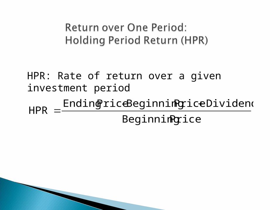
HPR: Rate of return over a given investment period

Price Beginning

DividendsPrice Beginning-Price EndingHPR

Ending Price = 110Beginning Price = 100Dividend = 4

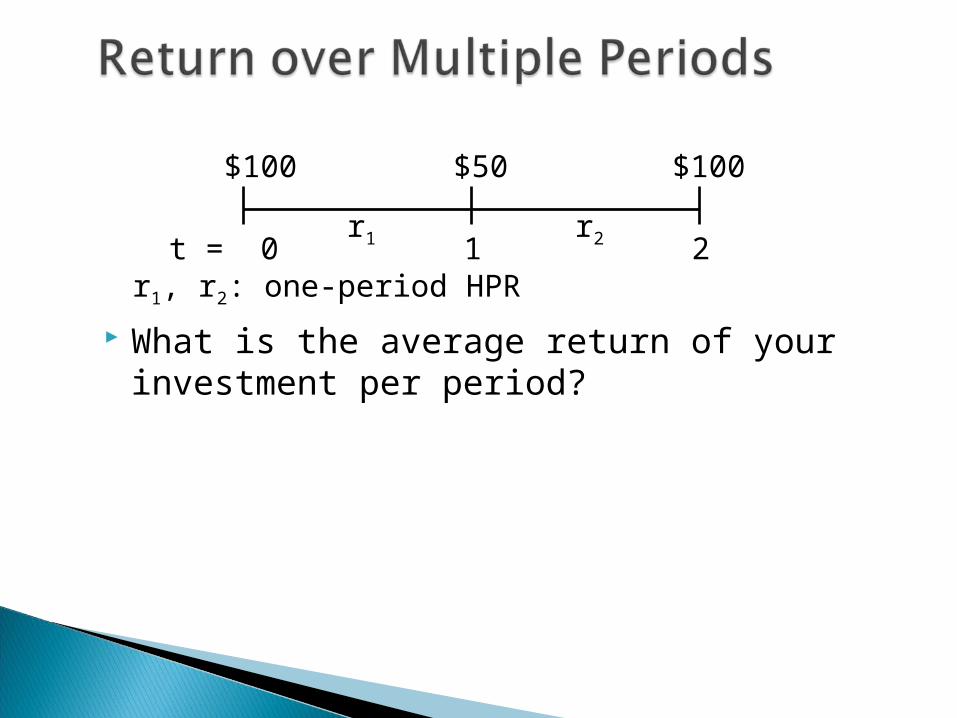
What is the average return of your investment per period?

t = 0 1 2

$100 $50 $100

r1 r2

r1, r2: one-period HPR

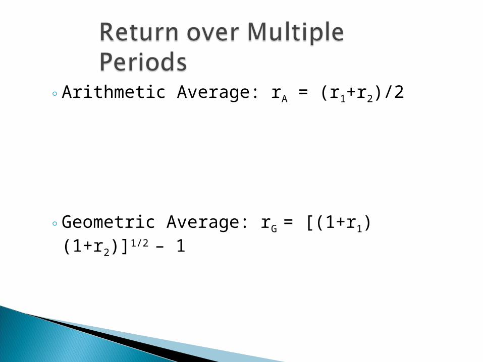
◦Arithmetic Average: rA = (r1+r2)/2

◦Geometric Average: rG = [(1+r1)(1+r2)]1/2 – 1

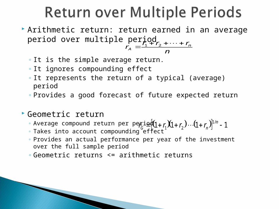
Arithmetic return: return earned in an average period over multiple period

◦ It is the simple average return. ◦ It ignores compounding effect◦ It represents the return of a typical (average) period◦ Provides a good forecast of future expected return

Geometric return◦ Average compound return per period◦ Takes into account compounding effect◦ Provides an actual performance per year of the investment over the full sample

period

◦ Geometric returns <= arithmetic returns

n

rrrr n

A

21

1111 /121 n

nG rrrr

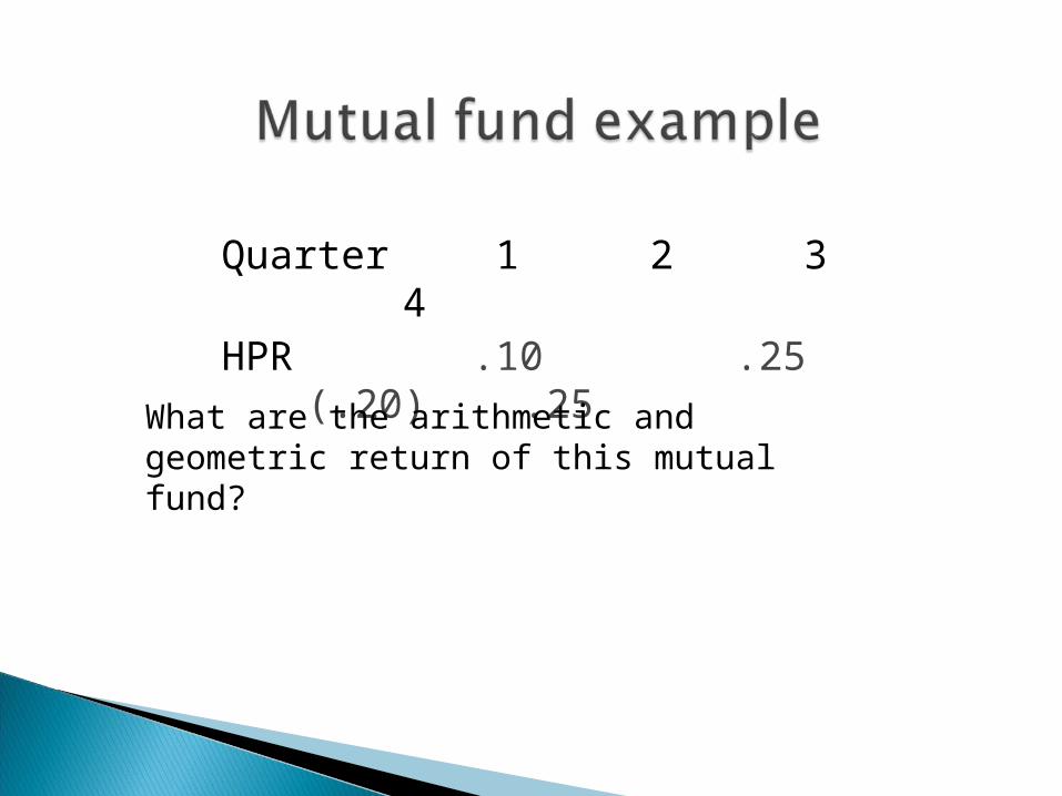
Quarter 1 2 3 4HPR .10 .25 (.20) .25

What are the arithmetic and geometric return of this mutual fund?

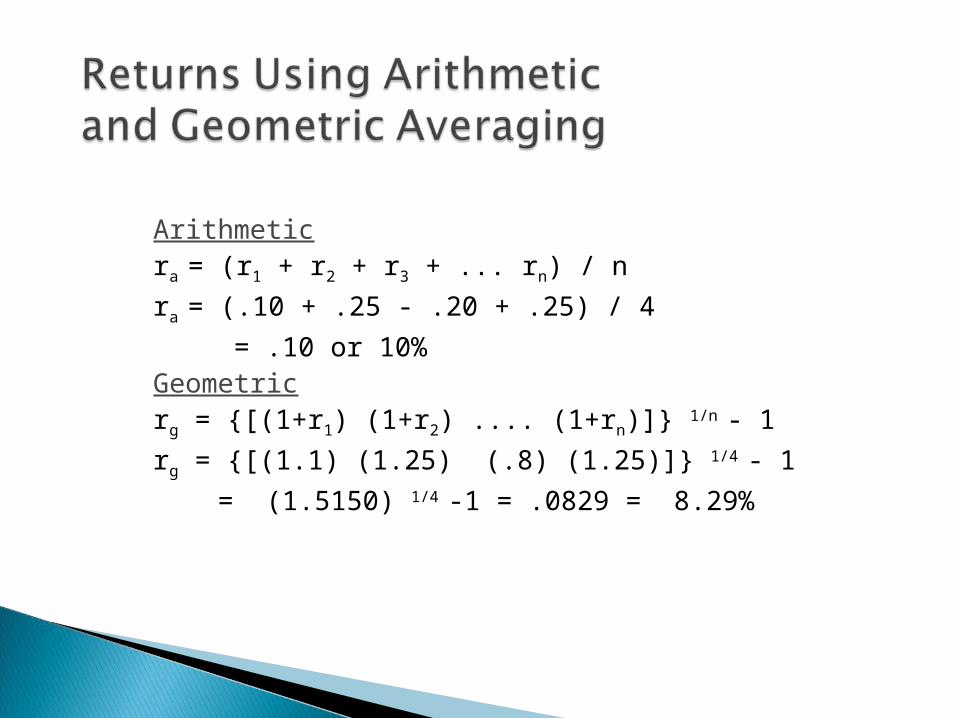
Arithmeticra = (r1 + r2 + r3 + ... rn) / n

ra = (.10 + .25 - .20 + .25) / 4

= .10 or 10%Geometricrg = {[(1+r1) (1+r2) .... (1+rn)]} 1/n - 1

rg = {[(1.1) (1.25) (.8) (1.25)]} 1/4 - 1

= (1.5150) 1/4 -1 = .0829 = 8.29%

Invest $1 into 2 investments: one gives 10% per year compounded annually, the other gives 10% compounded semi-annually. Which one gives higher return

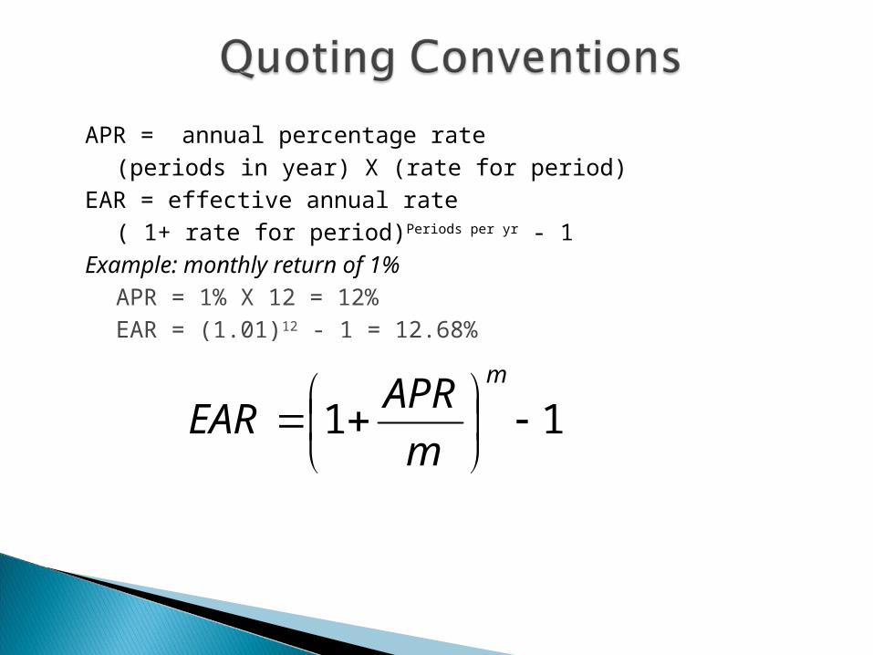
APR = annual percentage rate(periods in year) X (rate for period)

EAR = effective annual rate( 1+ rate for period)Periods per yr - 1

Example: monthly return of 1%APR = 1% X 12 = 12%EAR = (1.01)12 - 1 = 12.68%

11

m

m

APREAR

Risk in finance: uncertainty related to outcomes of an investment◦ The higher uncertainty, the riskier the investment.◦ How to measure risk and return in the future

Probability distribution: list of all possible outcomes and probability associated with each outcome, and sum of all prob. = 1.

For any distribution, the 2 most important characteristics◦ Mean◦ Standard deviation

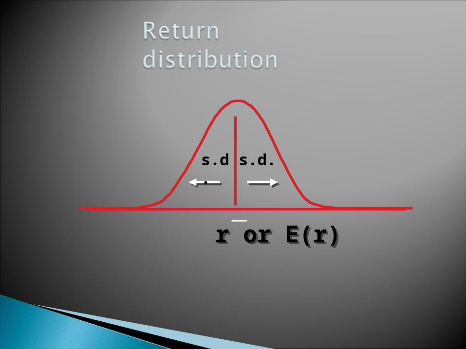
r or E(r)r or E(r)

s.d. s.d.

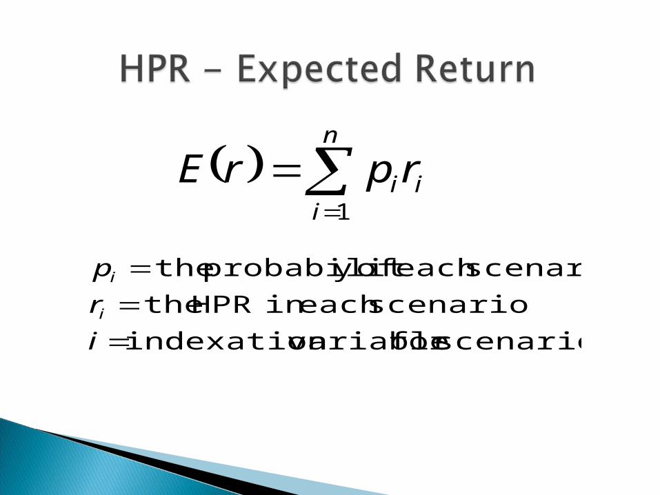
n

iiirprE

1

scenariosfor variableindexation

scenarioeach in HPR the

scenarioeach ofy probabilit the

i

r

p

i

i

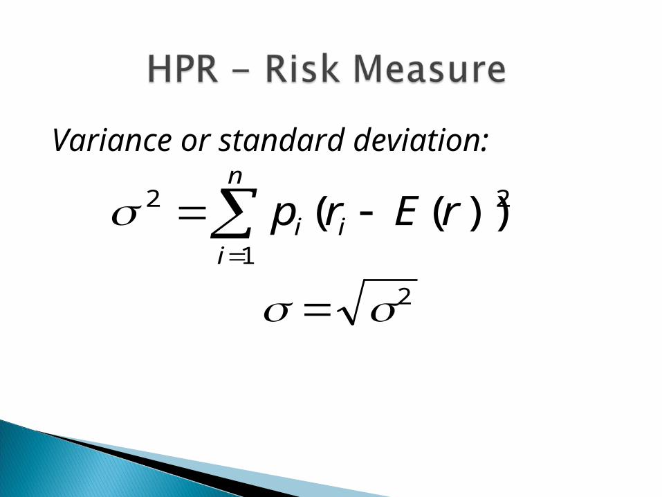
Variance or standard deviation:

n

iii rErp

1

22 ))((

2

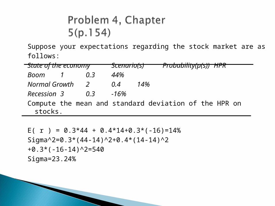
Suppose your expectations regarding the stock market are as

follows:

State of the economy Scenario(s) Probability(p(s)) HPR

Boom 1 0.3 44%

Normal Growth 2 0.4 14%

Recession 3 0.3 -16%

Compute the mean and standard deviation of the HPR on stocks.

E( r ) = 0.3*44 + 0.4*14+0.3*(-16)=14%

Sigma^2=0.3*(44-14)^2+0.4*(14-14)^2

+0.3*(-16-14)^2=540

Sigma=23.24%

-5 -4 -3 -2 -1 0 1 2 3 4 50

0.05

0.1

0.15

0.2

0.25

0.3

0.35

0.4

Outcomes

Probability

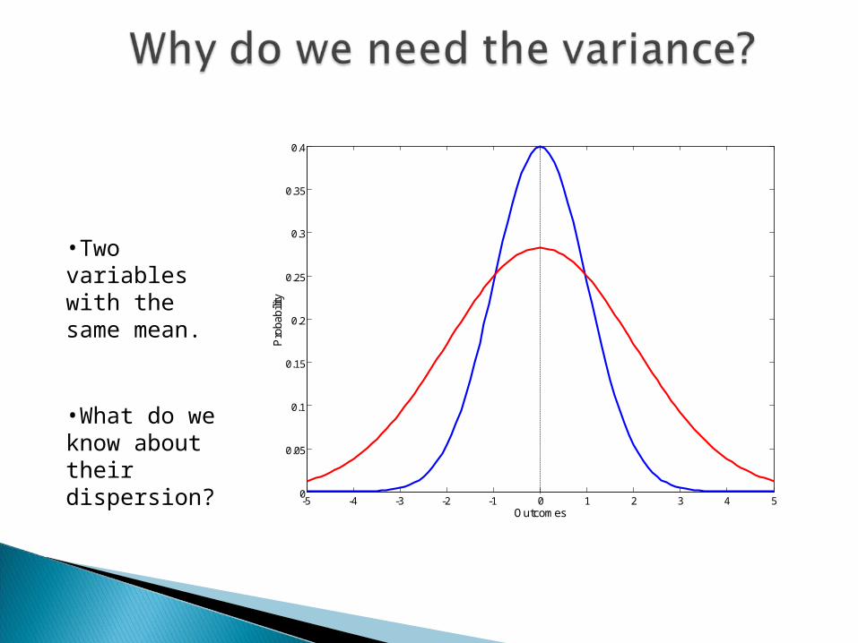
•Two variables with the same mean.

•What do we know about their dispersion?

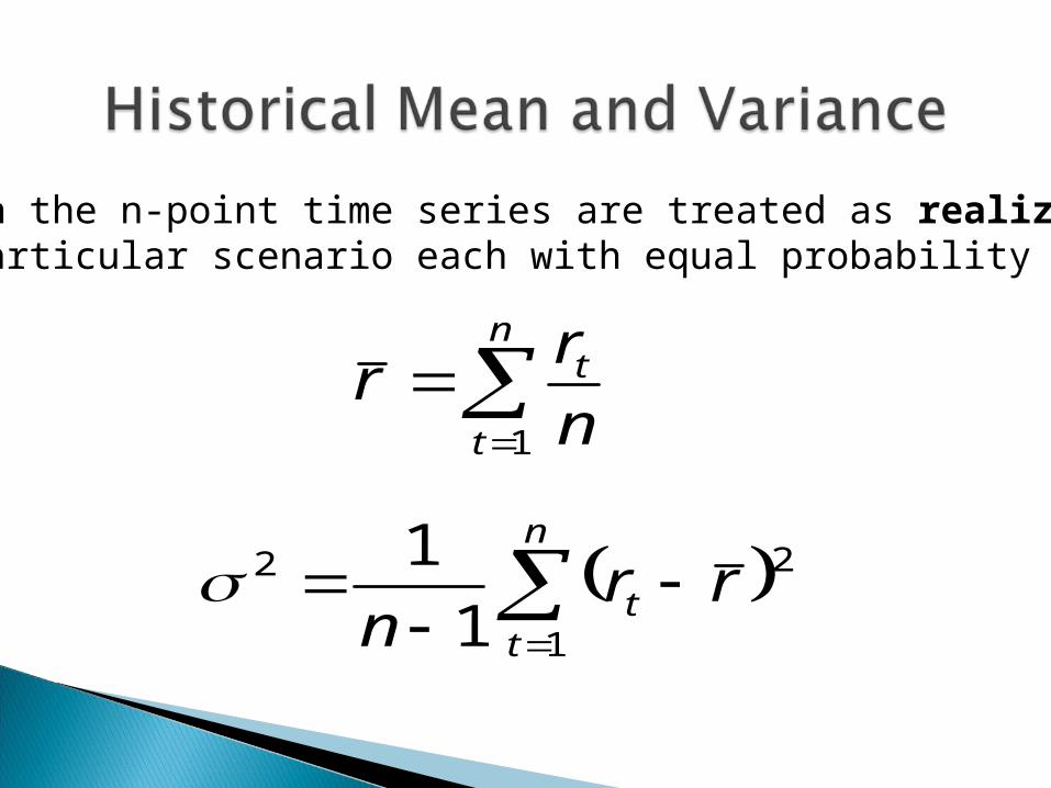
Data in the n-point time series are treated as realization of a particular scenario each with equal probability 1/n

n

t

t

n

rr

1

n

tt rr

n 1

22

1

1

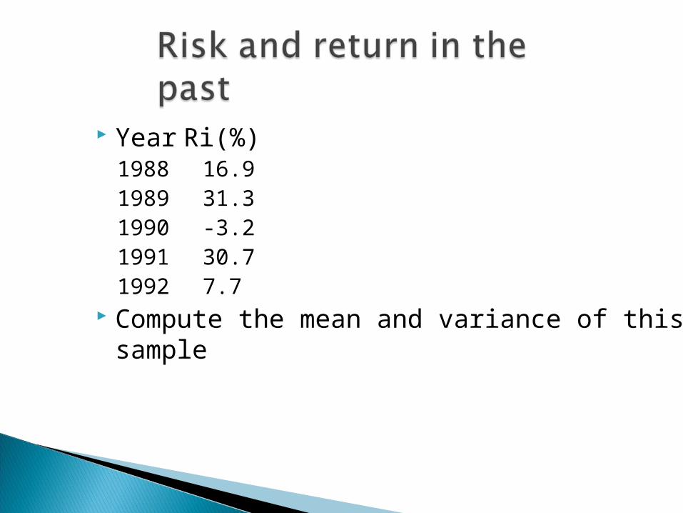
Year Ri(%)1988 16.91989 31.31990 -3.21991 30.71992 7.7

Compute the mean and variance of this sample

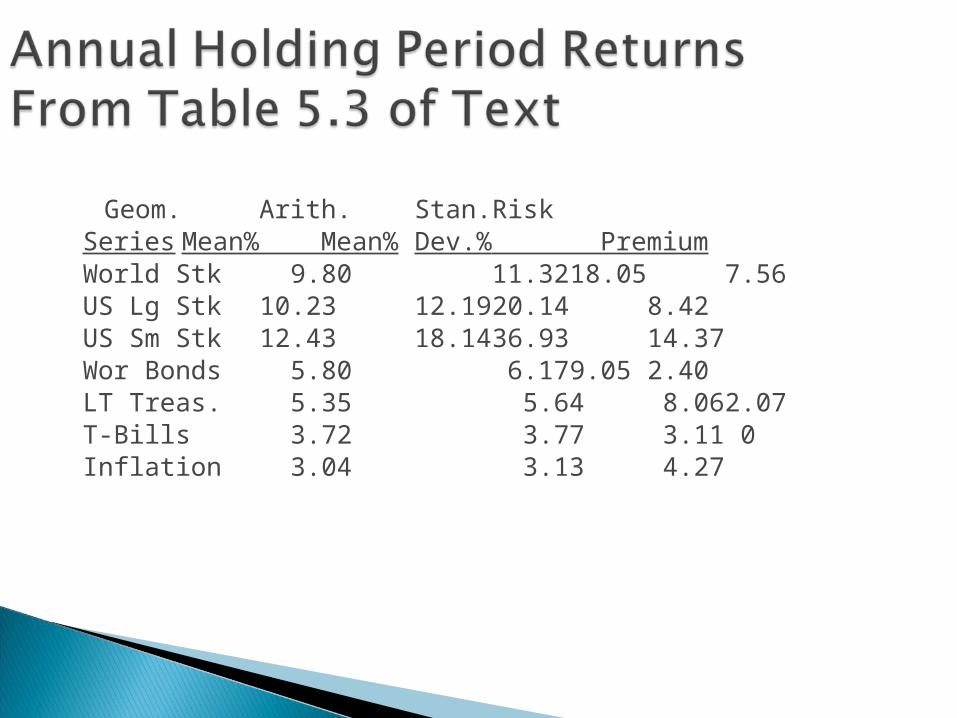
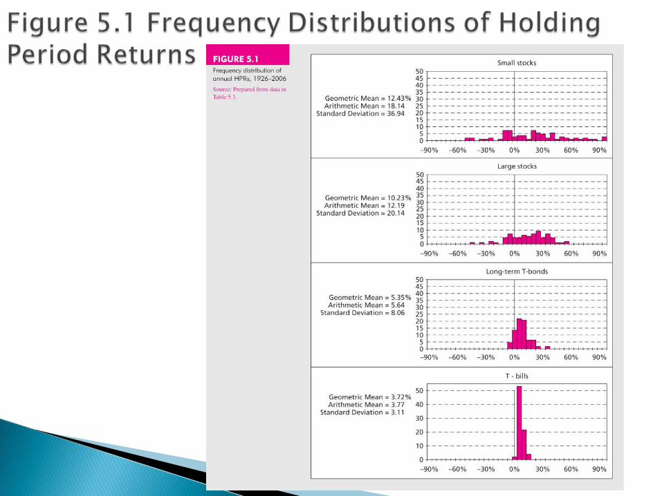
Geom. Arith. Stan. RiskSeries Mean% Mean% Dev.% PremiumWorld Stk 9.80 11.32 18.05 7.56US Lg Stk 10.23 12.19 20.14 8.42US Sm Stk 12.43 18.14 36.93 14.37Wor Bonds 5.80 6.17 9.05 2.40LT Treas. 5.35 5.64 8.06 2.07T-Bills 3.72 3.77 3.11 0Inflation 3.04 3.13 4.27

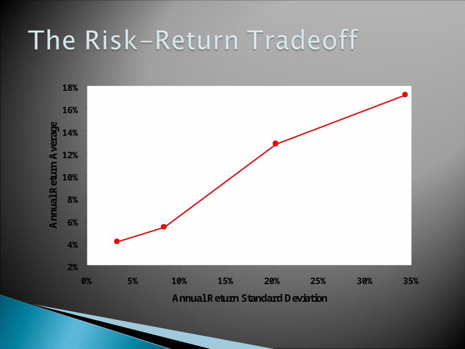
2%

4%

6%

8%

10%

12%

14%

16%

18%

0% 5% 10% 15% 20% 25% 30% 35%

Annual Return Standard Deviation

Ann

ual R

etur

n A

vera

ge

T-Bonds

T-Bills

Large-Company Stocks

Small-Company Stocks

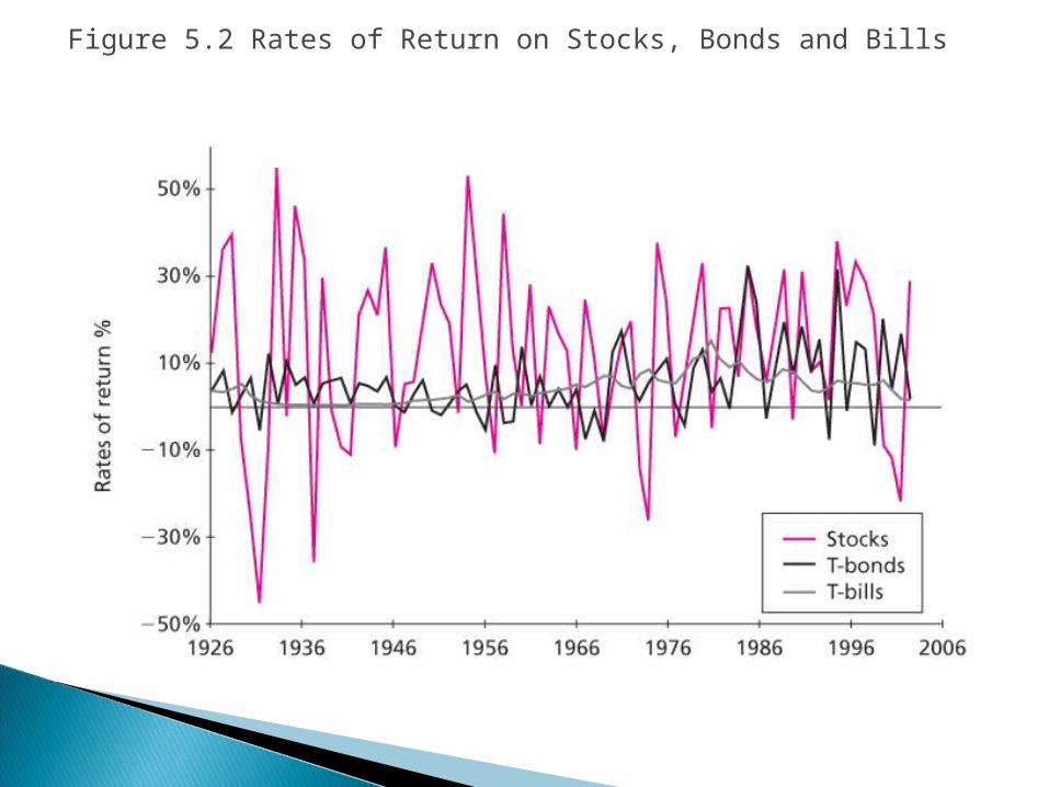
Figure 5.2 Rates of Return on Stocks, Bonds and Bills

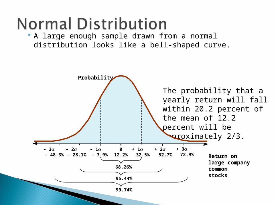
A large enough sample drawn from a normal distribution looks like a bell-shaped curve.

Probability

Return onlarge company commonstocks

99.74%

– 3 – 48.3%

– 2 – 28.1%

– 1 – 7.9%

012.2%

+ 1 32.5%

+ 2 52.7%

+ 3 72.9%

The probability that a yearly return will fall within 20.2 percent of the mean of 12.2 percent will be approximately 2/3.

68.26%

95.44%

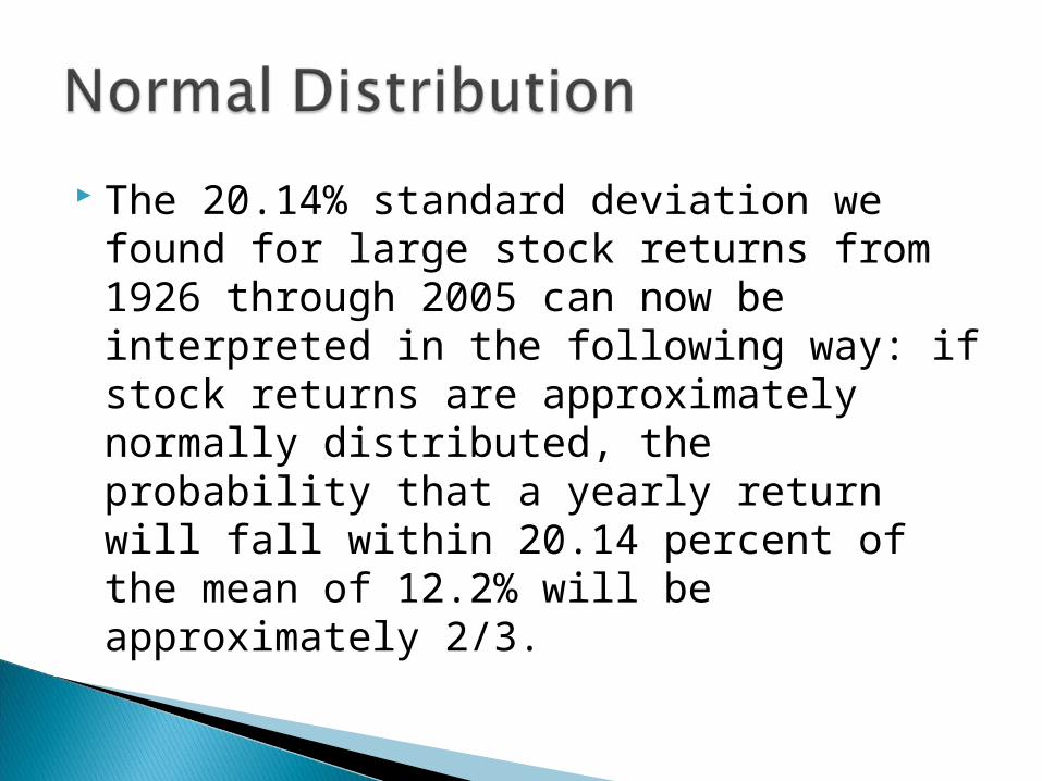
The 20.14% standard deviation we found for large stock returns from 1926 through 2005 can now be interpreted in the following way: if stock returns are approximately normally distributed, the probability that a yearly return will fall within 20.14 percent of the mean of 12.2% will be approximately 2/3.

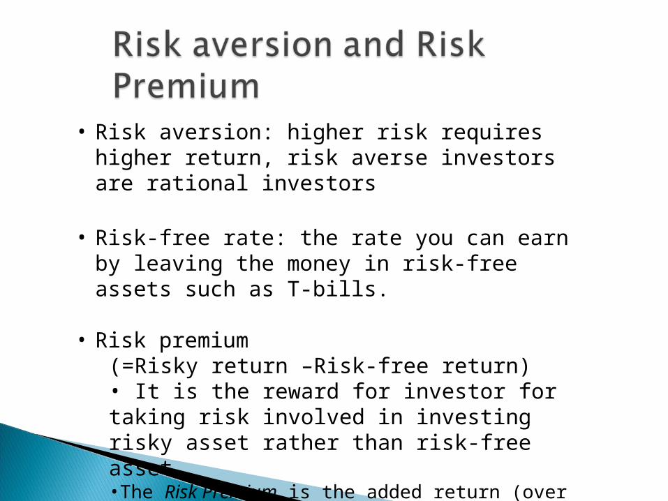
• Risk aversion: higher risk requires higher return, risk averse investors are rational investors

• Risk-free rate: the rate you can earn by leaving the money in risk-free assets such as T-bills.

• Risk premium(=Risky return –Risk-free return)• It is the reward for investor for taking risk involved in investing risky asset rather than risk-free asset.•The Risk Premium is the added return (over and above the risk-free rate) resulting from bearing risk.

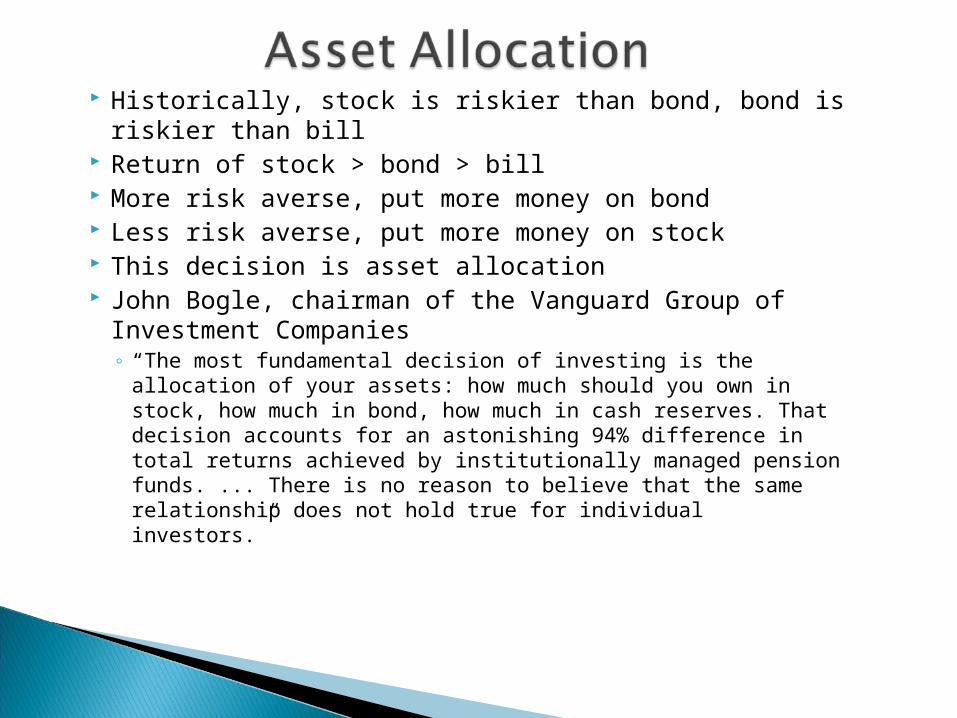
Historically, stock is riskier than bond, bond is riskier than bill Return of stock > bond > bill More risk averse, put more money on bond Less risk averse, put more money on stock This decision is asset allocation John Bogle, chairman of the Vanguard Group of Investment

Companies◦ “The most fundamental decision of investing is the allocation of your

assets: how much should you own in stock, how much in bond, how much in cash reserves. That decision accounts for an astonishing 94% difference in total returns achieved by institutionally managed pension funds. ... There is no reason to believe that the same relationship does not hold true for individual investors.”

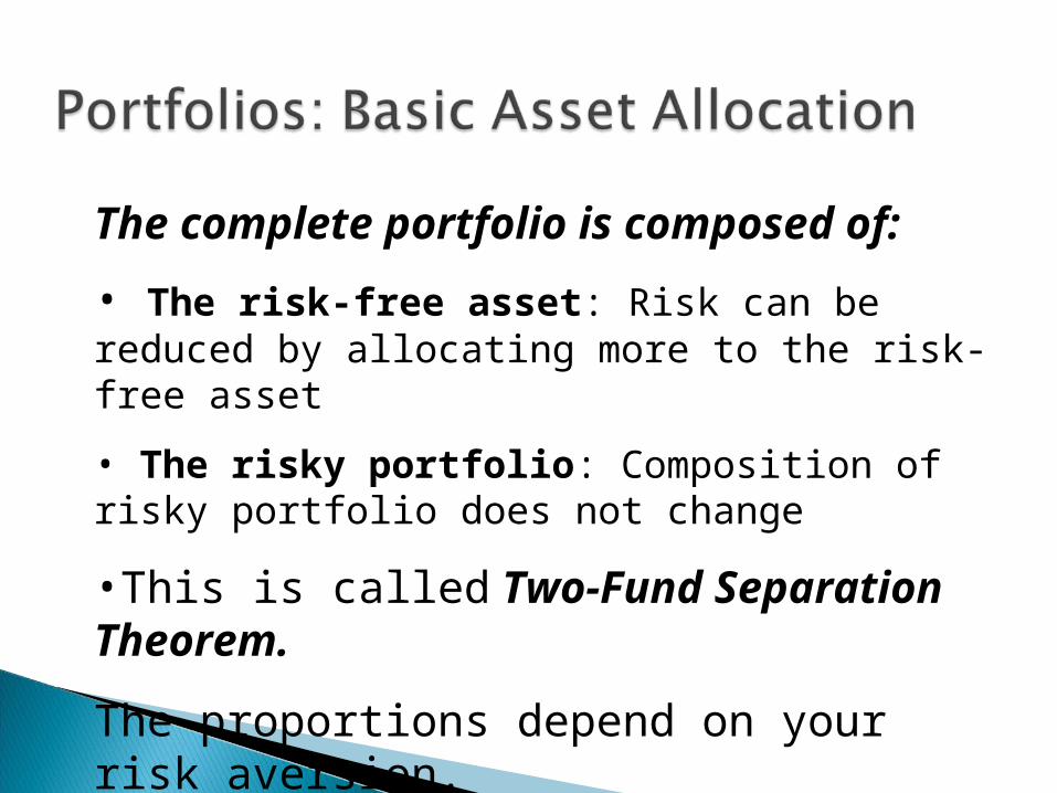
The complete portfolio is composed of:

• The risk-free asset: Risk can be reduced by allocating more to the risk-free asset

• The risky portfolio: Composition of risky portfolio does not change

•This is called Two-Fund Separation Theorem.

The proportions depend on your risk aversion.

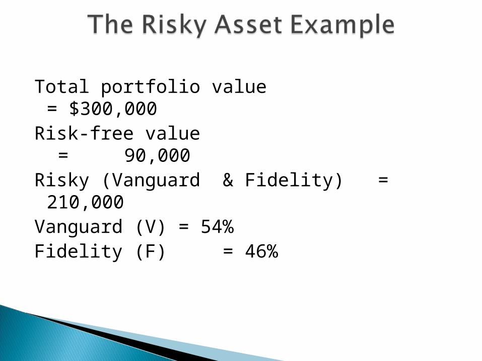
Total portfolio value = $300,000Risk-free value = 90,000Risky (Vanguard & Fidelity) = 210,000Vanguard (V) = 54% Fidelity (F) = 46%

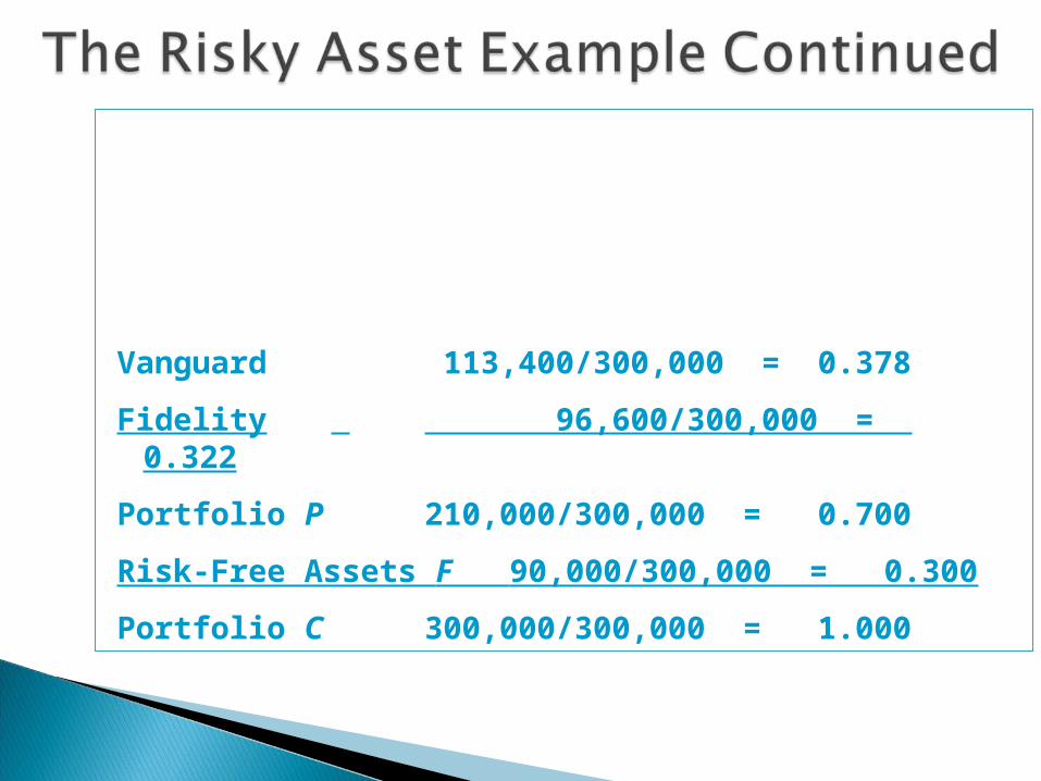
Vanguard 113,400/300,000 = 0.378

Fidelity 96,600/300,000 = 0.322

Portfolio P 210,000/300,000 = 0.700

Risk-Free Assets F 90,000/300,000 = 0.300

Portfolio C 300,000/300,000 = 1.000

Only the government can issue default-free bonds◦Guaranteed real rate only if the duration of the bond is identical to the investor’s desire holding period

T-bills viewed as the risk-free asset◦Less sensitive to interest rate fluctuations

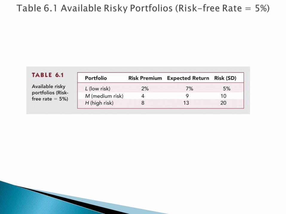
It’s possible to split investment funds between safe and risky assets.

Risk free asset: proxy; T-bills Risky asset: stock (or a portfolio)

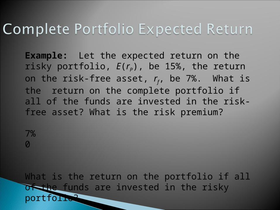
Example: Let the expected return on the risky portfolio, E(rP), be 15%, the return on the risk-free asset, rf, be 7%. What is the return on the complete portfolio if all of the funds are invested in the risk-free asset? What is the risk premium?

7%0

What is the return on the portfolio if all of the funds are invested in the risky portfolio?

15%8%

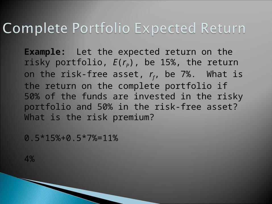
Example: Let the expected return on the risky portfolio, E(rP), be 15%, the return on the risk-free asset, rf, be 7%. What is the return on the complete portfolio if 50% of the funds are invested in the risky portfolio and 50% in the risk-free asset? What is the risk premium?

0.5*15%+0.5*7%=11%

4%

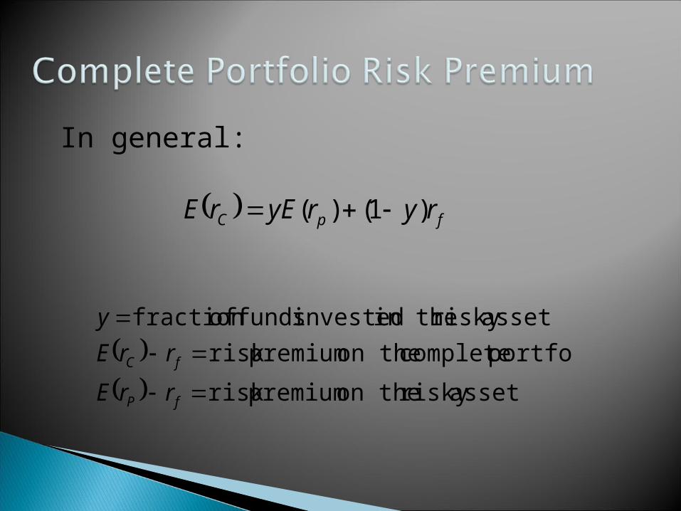
fpC ryryErE )1()(

assetrisky on the premiumrisk

portfolio complete on the premiumrisk

assetrisky in the invested funds offraction

fP

fC

rrE

rrE

y

In general:

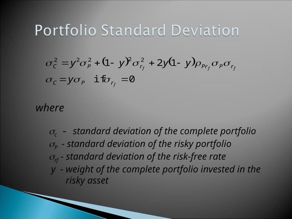
0 if

121 22222

f

fff

rPC

rPPrrPC

y

yyyy

where

c - standard deviation of the complete portfolioP - standard deviation of the risky portfoliorf - standard deviation of the risk-free rate y - weight of the complete portfolio invested in the risky asset

Example: Let the standard deviation on the risky portfolio, P, be 22%. What is the standard deviation of the complete portfolio if 50% of the funds are invested in the risky portfolio and 50% in the risk-free asset?

22%*0.5=11%

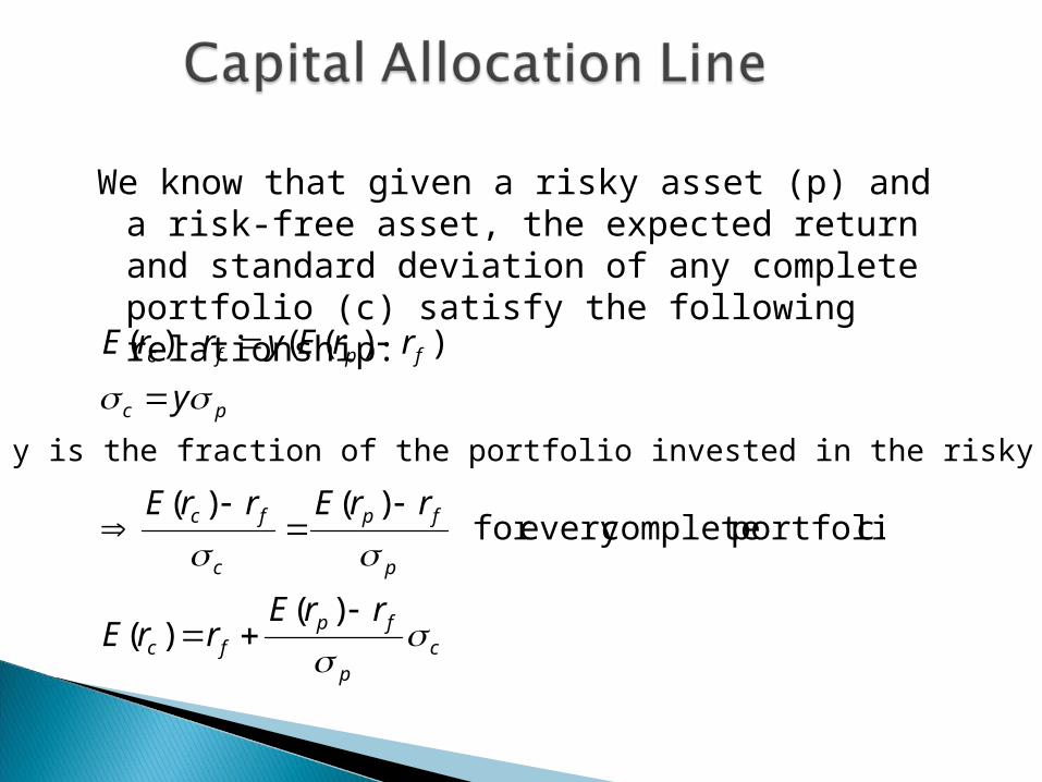
We know that given a risky asset (p) and a risk-free asset, the expected return and standard deviation of any complete portfolio (c) satisfy the following relationship:

cp

fpfc

p

fp

c

fc

pc

fpfc

rrErrE

rrErrE

y

rrEyrrE

)()(

c portfolio completeevery for )()(

))(()(

Where y is the fraction of the portfolio invested in the risky asset

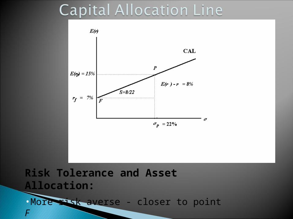
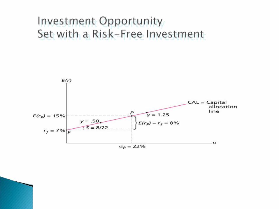
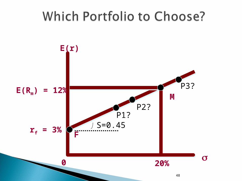
Risk Tolerance and Asset Allocation:

•More risk averse - closer to point F

•Less risk averse - closer to P

S

E r rP f

P

S is the increase in expected return per unit of additional standard deviation

S is the reward-to-variability ratio or Sharpe Ratio

Example: Let the expected return on the risky portfolio, E(rP),

be 15%, the return on the risk-free asset, rf, be 7% and the

standard deviation on the risky portfolio, P, be 22%. What is

the slope of the CAL for the complete portfolio?

S = (15%-7%)/22% = 8/22

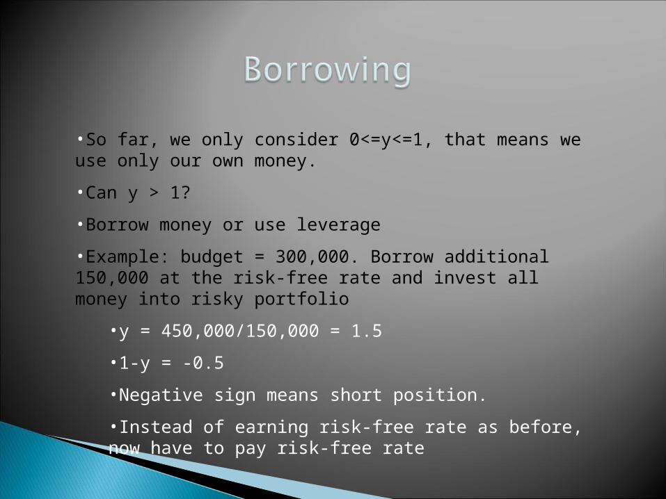
•So far, we only consider 0<=y<=1, that means we use only our own money.

•Can y > 1?

•Borrow money or use leverage

•Example: budget = 300,000. Borrow additional 150,000 at the risk-free rate and invest all money into risky portfolio

•y = 450,000/150,000 = 1.5

•1-y = -0.5

•Negative sign means short position.

•Instead of earning risk-free rate as before, now have to pay risk-free rate

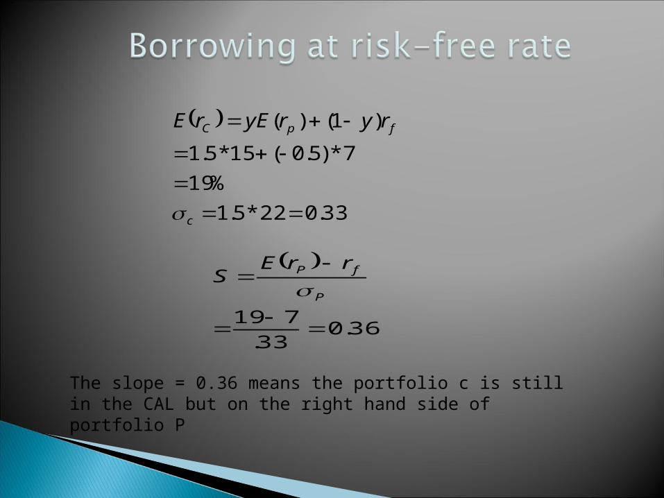
33.022*5.1

%19

7*)5.0(15*5.1

)1()(

c

fpC ryryErE

36.033.

719

P

fP rrES

The slope = 0.36 means the portfolio c is still in the CAL but on the right hand side of portfolio P

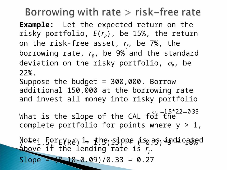
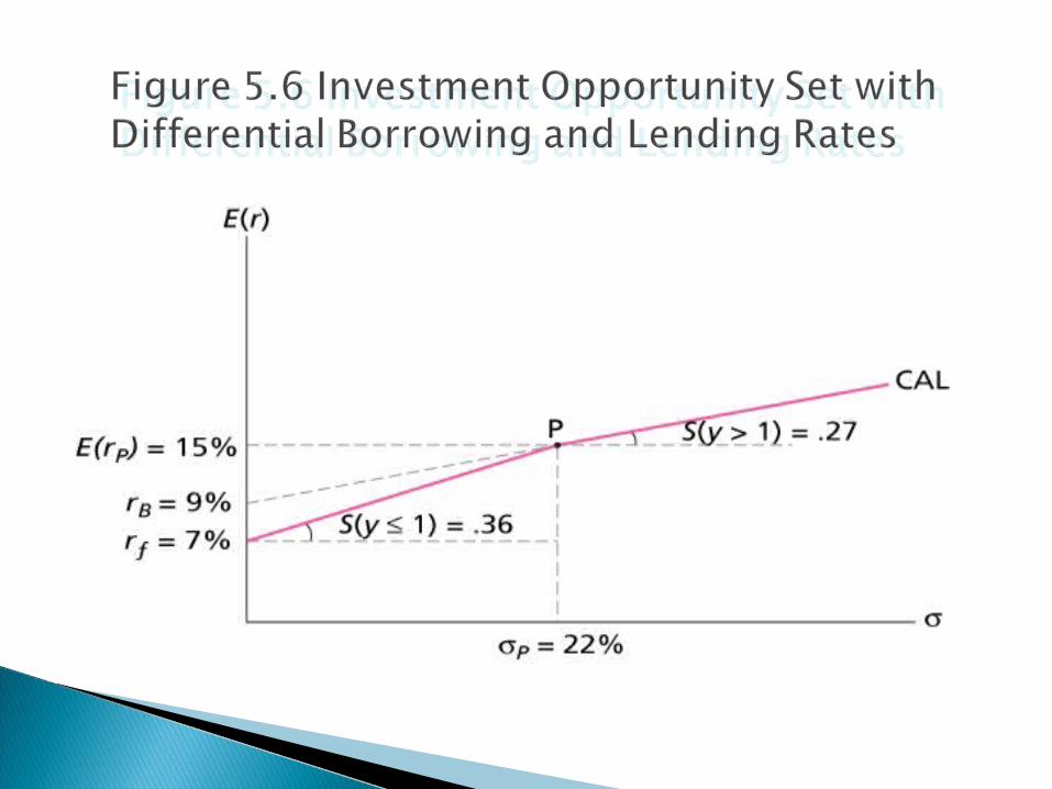
Example: Let the expected return on the risky portfolio, E(rP), be 15%, the return on the risk-free asset, rf, be 7%, the borrowing rate, rB, be 9% and the standard deviation on the risky portfolio, P, be 22%. Suppose the budget = 300,000. Borrow additional 150,000 at the borrowing rate and invest all money into risky portfolio

What is the slope of the CAL for the complete portfolio for points where y > 1,

y = 1.5; E(Rc) = 1.5(15) + (-0.5)*9 = 18%

Slope = (0.18-0.09)/0.33 = 0.27Note: For y 1, the slope is as indicated above if the lending rate is rf.

33.022*5.1 c

SPECIAL CASE OF CAL (I.e., P=MKT)

The line provided by one-month T-bills and a broad index of common stocks (e.g. S&P500)

Consequence of a passive investment strategy based on stocks and T-bills

48

E(r)

E(Rm) = 12%

rf = 3%

20%0

M

F

S=0.45P1?

P3?

P2?

FIN 8330 Lecture 7 10/04/07 49

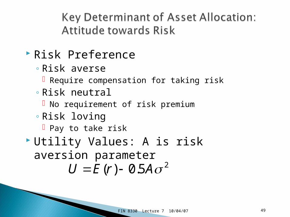
Risk Preference ◦ Risk averse

Require compensation for taking risk

◦ Risk neutral No requirement of risk premium

◦ Risk loving Pay to take risk

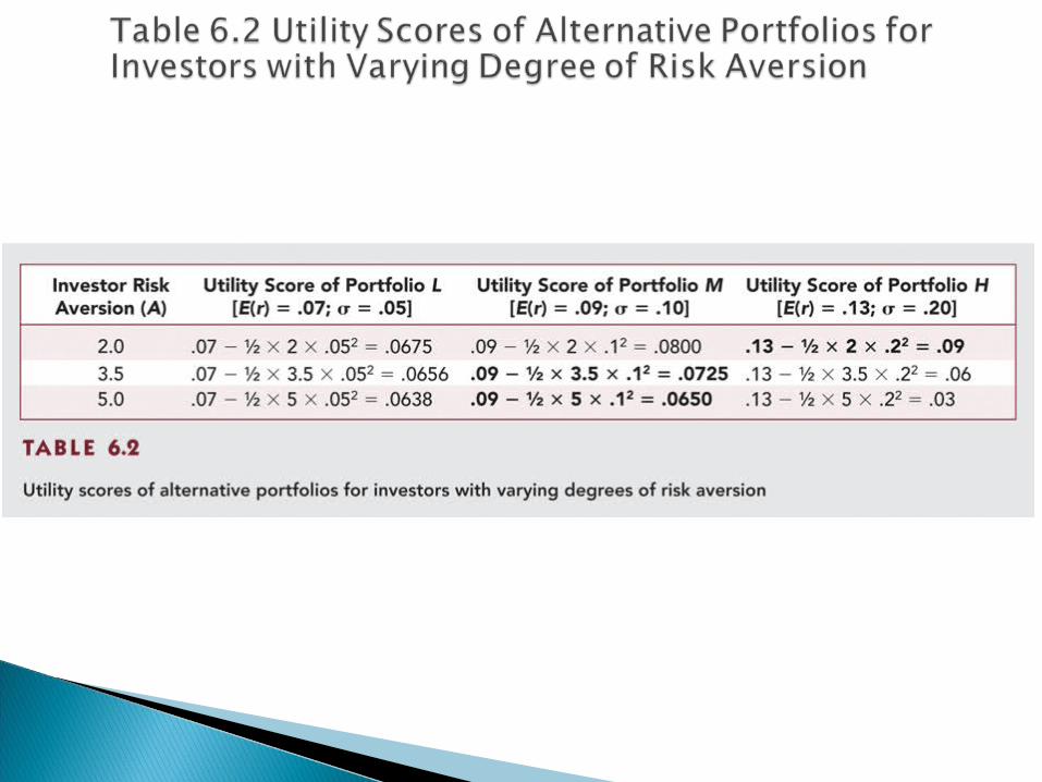
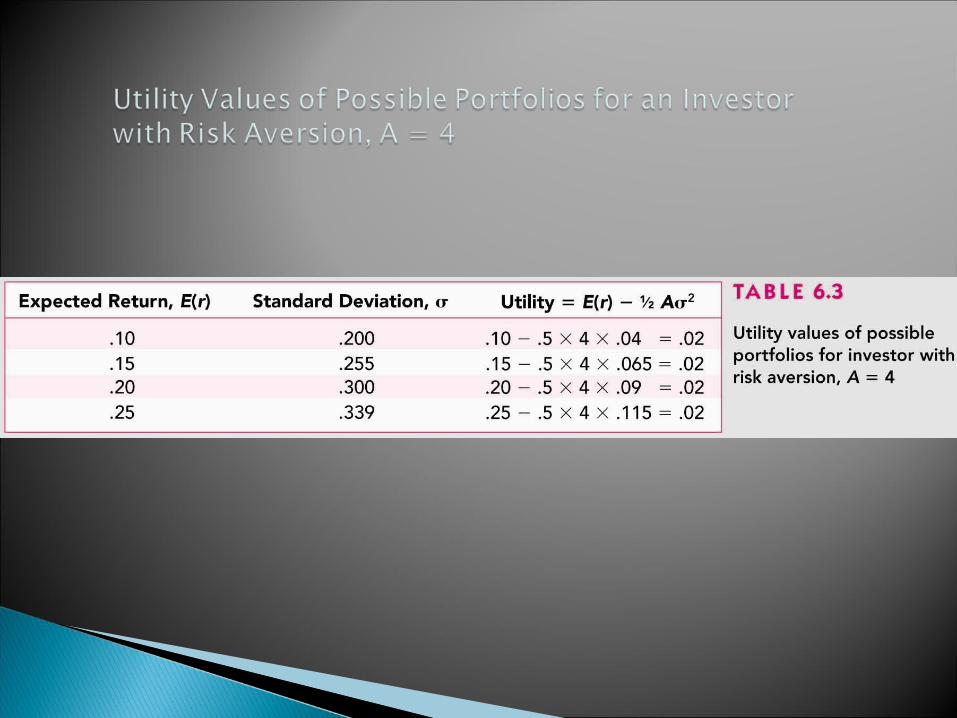
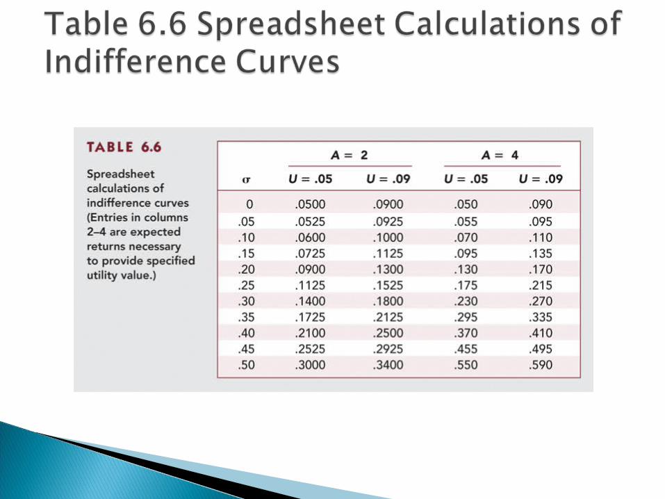
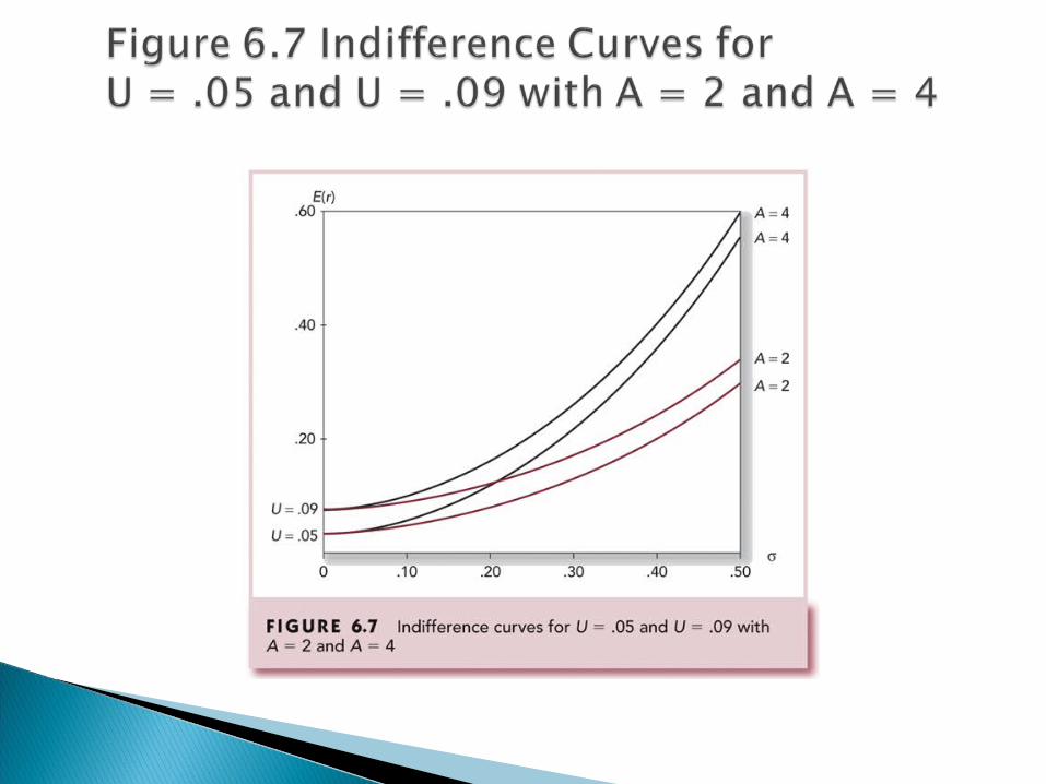
Utility Values: A is risk aversion parameter

25.0)( ArEU

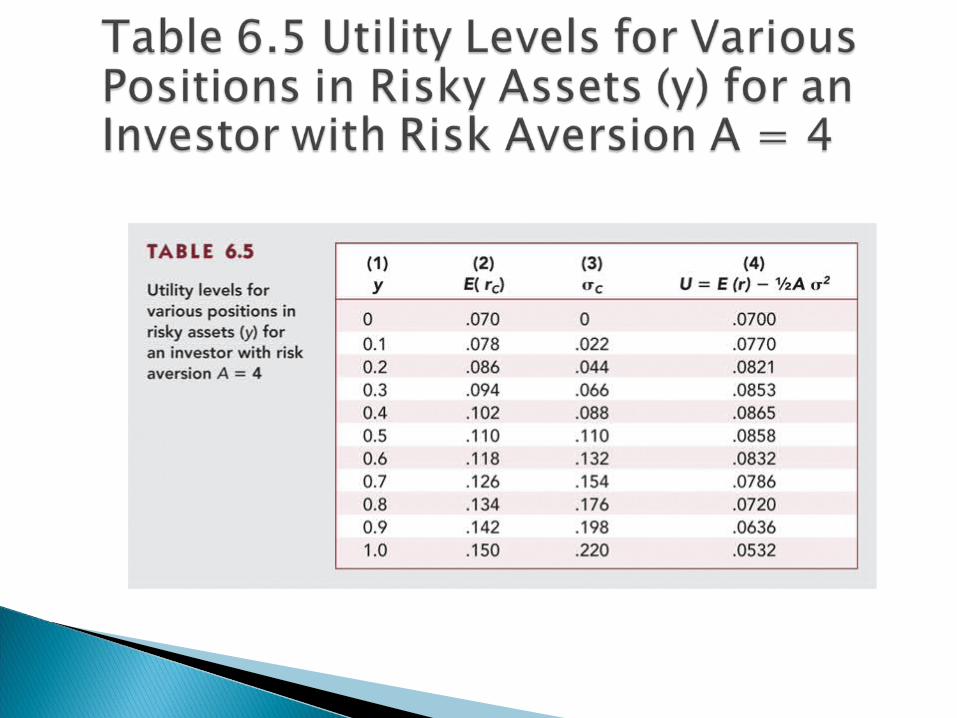
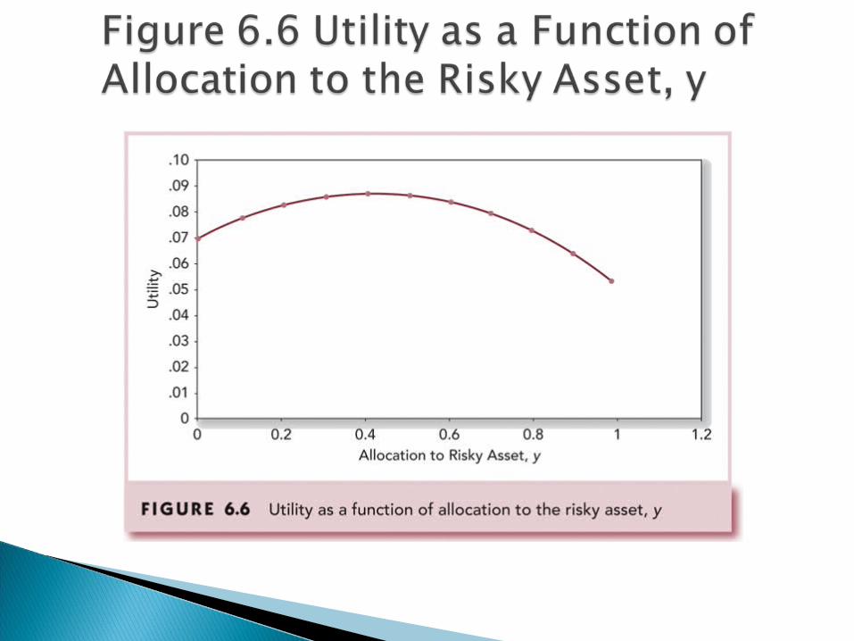
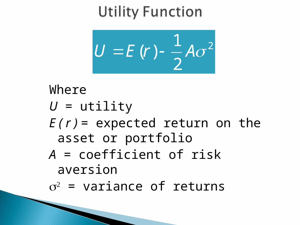
WhereU = utilityE ( r ) = expected return on the

asset or portfolioA = coefficient of risk aversion = variance of returns

21( )

2U E r A

55

Greater levels of risk aversion lead to larger proportions of the risk free rate.

Lower levels of risk aversion lead to larger proportions of the portfolio of risky assets.

Willingness to accept high levels of risk for high levels of returns would result in leveraged combinations.

56

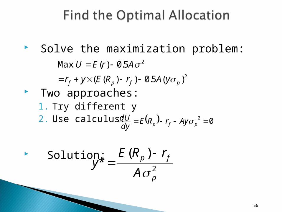
Solve the maximization problem:

Two approaches: 1. Try different y2. Use calculus:

Solution:

2

2

)(5.0))((

5.0)(Max

pfpf yArREyr

ArEU

02 pfp AyrREdydU

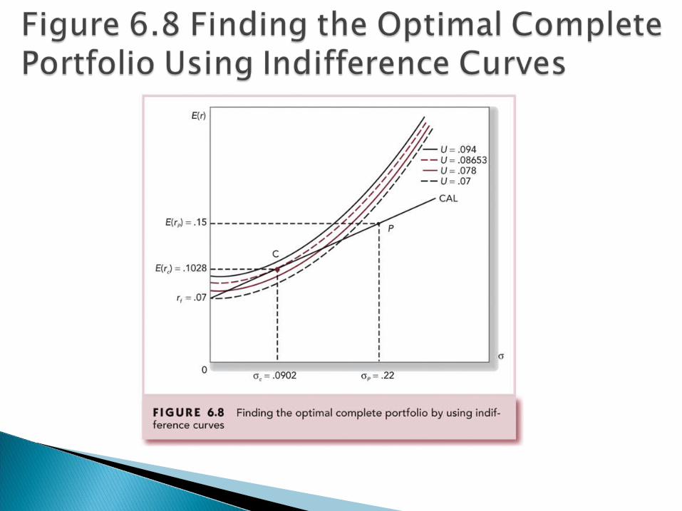
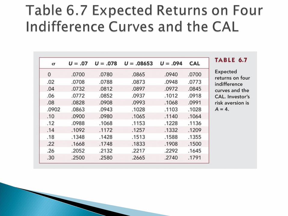
2

)(*

p

fp

A

rREy

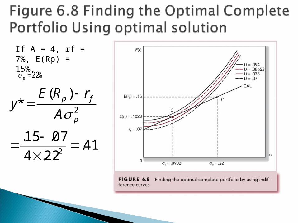
If A = 4, rf = 7%, E(Rp) = 15%,

%22p

41.22.4

07.15.

)(*

2

2

p

fp

A

rREy

58

FIN 8330 Lecture 7 10/04/07 66

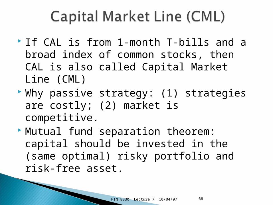
If CAL is from 1-month T-bills and a broad index of common stocks, then CAL is also called Capital Market Line (CML)

Why passive strategy: (1) strategies are costly; (2) market is competitive.

Mutual fund separation theorem: capital should be invested in the (same optimal) risky portfolio and risk-free asset.

Passive strategy involves a decision that avoids any direct or indirect security analysis

Supply and demand forces may make such a strategy a reasonable choice for many investors

A natural candidate for a passively held risky asset would be a well-diversified portfolio of common stocks

Because a passive strategy requires devoting no resources to acquiring information on any individual stock or group we must follow a “neutral” diversification strategy

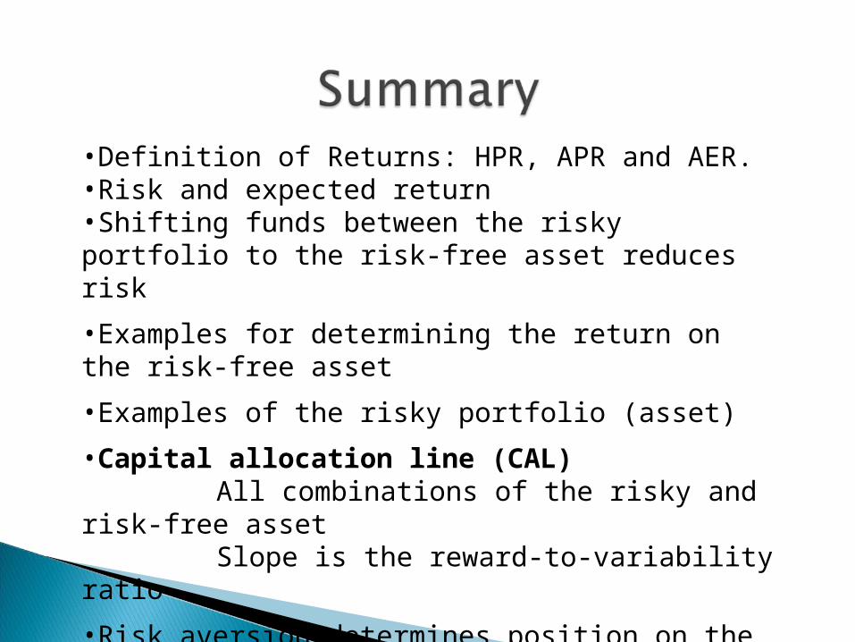
•Definition of Returns: HPR, APR and AER.•Risk and expected return •Shifting funds between the risky portfolio to the risk-free asset reduces risk

•Examples for determining the return on the risk-free asset

•Examples of the risky portfolio (asset)

•Capital allocation line (CAL) All combinations of the risky and risk-free asset Slope is the reward-to-variability ratio

•Risk aversion determines position on the capital allocation line