risk management adequacy

RISK MANAGEMENTAND CAPITALADEQUACY

Gallati_fm_1p_j.qxd 2/27/03 9:15 AM Page i

Administrator

打字机

ebook3600.com

This page intentionally left blank.

RISK MANAGEMENTAND CAPITALADEQUACY

RETO R. GALLATI

McGraw-HillNew York / Chicago / San Francisco / Lisbon

London / Madrid / Mexico City / Milan / New Delhi

San Juan / Singapore / Sydney / Toronto

Gallati_fm_1p_j.qxd 2/27/03 9:15 AM Page iii

Copyright © 2003 by The McGraw-Hill Companies, Inc. All rights reserved. Manufactured in theUnited States of America. Except as permitted under the United States Copyright Act of 1976, no partof this publication may be reproduced or distributed in any form or by any means, or stored in a data-base or retrieval system, without the prior written permission of the publisher.

0-07-142558-6

The material in this eBook also appears in the print version of this title: 0-07-140763-4.

All trademarks are trademarks of their respective owners. Rather than put a trademark symbol afterevery occurrence of a trademarked name, we use names in an editorial fashion only, and to the benefitof the trademark owner, with no intention of infringement of the trademark. Where such designationsappear in this book, they have been printed with initial caps.

McGraw-Hill eBooks are available at special quantity discounts to use as premiums and sales pro-motions, or for use in corporate training programs. For more information, please contact GeorgeHoare, Special Sales, at [email protected] or (212) 904-4069.

TERMS OF USEThis is a copyrighted work and The McGraw-Hill Companies, Inc. (“McGraw-Hill”) and its licensorsreserve all rights in and to the work. Use of this work is subject to these terms. Except as permittedunder the Copyright Act of 1976 and the right to store and retrieve one copy of the work, you may notdecompile, disassemble, reverse engineer, reproduce, modify, create derivative works based upon,transmit, distribute, disseminate, sell, publish or sublicense the work or any part of it withoutMcGraw-Hill’s prior consent. You may use the work for your own noncommercial and personal use;any other use of the work is strictly prohibited. Your right to use the work may be terminated if youfail to comply with these terms.

THE WORK IS PROVIDED “AS IS”. McGRAW-HILL AND ITS LICENSORS MAKE NO GUAR-ANTEES OR WARRANTIES AS TO THE ACCURACY, ADEQUACY OR COMPLETENESS OFOR RESULTS TO BE OBTAINED FROM USING THE WORK, INCLUDING ANY INFORMA-TION THAT CAN BE ACCESSED THROUGH THE WORK VIA HYPERLINK OR OTHERWISE,AND EXPRESSLY DISCLAIM ANY WARRANTY, EXPRESS OR IMPLIED, INCLUDING BUTNOT LIMITED TO IMPLIED WARRANTIES OF MERCHANTABILITY OR FITNESS FOR APARTICULAR PURPOSE. McGraw-Hill and its licensors do not warrant or guarantee that the func-tions contained in the work will meet your requirements or that its operation will be uninterrupted orerror free. Neither McGraw-Hill nor its licensors shall be liable to you or anyone else for any inac-curacy, error or omission, regardless of cause, in the work or for any damages resulting therefrom.McGraw-Hill has no responsibility for the content of any information accessed through the work.Under no circumstances shall McGraw-Hill and/or its licensors be liable for any indirect, incidental,special, punitive, consequential or similar damages that result from the use of or inability to use thework, even if any of them has been advised of the possibility of such damages. This limitation of lia-bility shall apply to any claim or cause whatsoever whether such claim or cause arises in contract, tortor otherwise.

DOI: 10.1036/0071425586

ebook_copyright 7x9.qxd 7/23/03 10:53 AM Page 1

When I was young, people called me a gambler. As thescale of my operations increased I became known as aspeculator. Now I am called a banker. But I have beendoing the same thing all the time.

—Sir Ernest CassellBanker to Edward VII

Gallati_fm_1p_j.qxd 2/27/03 9:15 AM Page v

To my parents with love and gratitude

Gallati_fm_1p_j.qxd 2/27/03 9:15 AM Page vii

A C K N O W L E D G M E N T S

The suggestion that I write a book about risk came from the late FischerBlack, while I was working at Goldman Sachs. The vastness of the projectis daunting. The topic touches on the most profound depths of statistics,mathematics, psychology, and economics. I would like to thank the editorsand reviewers and those who provided comments, especially M.R. Careyand Jean Eske, who carefully read the entire manuscript and providedvaluable comments, corrections, and advice.

I end with a note of thanks to my family, my friends, and my facultycolleagues at Sloan, who inspired much of the enthusiasm that went intothe creation of this book and endured me with patience.

RETO R. GALLATI

Cambridge, MassachusettsFebruary 2003

Gallati_fm_1p_j.qxd 2/28/03 2:10 PM Page viii

Copyright 2003 by The McGraw-Hill Companies, Inc. Click Here for Terms of Use.

C O N T E N T S

ACKNOWLEDGMENTS viii

INTRODUCTION xvii

Chapter 1

Risk Management: A Maturing Discipline 1

1.1 Background 11.2 Risks: A View of the Past Decades 51.3 Definition of Risk 71.4 Related Terms and Differentiation 81.5 Degree of Risk 101.6 Risk Management: A Multilayered Term 11

1.6.1 Background 111.6.2 History of Modern Risk Management 111.6.3 Related Approaches 131.6.4 Approach and Risk Maps 22

1.7 Systemic Risk 221.7.1 Definition 221.7.2 Causes of Systemic Risk 261.7.3 Factors That Support Systemic Risk 261.7.4 Regulatory Mechanisms for Risk Management 27

1.8 Summary 281.9 Notes 30

Chapter 2

Market Risk 33

2.1 Background 332.2 Definition of Market Risk 342.3 Conceptual Approaches for Modeling Market Risk 372.4 Modern Portfolio Theory 39

2.4.1 The Capital Asset Pricing Model 412.4.2 The Security Market Line 43

ix

Gallati_fm_1p_j.qxd 2/28/03 2:10 PM Page ix

For more information about this title, click here.


2.4.3 Modified Form of CAPM by Black, Jensen, and Scholes 452.4.4 Arbitrage Pricing Theory 462.4.5 Approaches to Option Pricing 47

2.5 Regulatory Initiatives for Market Risks and Value at Risk 542.5.1 Development of an International Framework

for Risk Regulation 562.5.2 Framework of the 1988 BIS Capital Adequacy Calculation 562.5.3 Criticisms of the 1988 Approach 582.5.4 Evolution of the 1996 Amendment on Market Risks 58

2.6 Amendment to the Capital Accord to Incorporate Market Risks 602.6.1 Scope and Coverage of Capital Charges 602.6.2 Countable Capital Components 612.6.3 The de Minimis Rule 62

2.7 The Standardized Measurement Method 622.7.1 General and Specific Risks for Equity- and

Interest-Rate-Sensitive Instruments 652.7.2 Interest-Rate Risks 662.7.3 Equity Position Risk 792.7.4 Foreign-Exchange Risk 832.7.5 Commodities Risk 842.7.6 Treatment of Options 882.7.7 Criticisms of the Standard Approach 94

2.8 The Internal Model Approach 952.8.1 Conditions for and Process of Granting Approval 952.8.2 VaR-Based Components and Multiplication Factor 972.8.3 Requirement for Specific Risks 982.8.4 Combination of Model-Based and Standard Approaches 982.8.5 Specification of Market Risk Factors to Be Captured 992.8.6 Minimum Quantitative Requirements 1012.8.7 Minimum Qualitative Requirements 102

2.9 The Precommitment Model 1072.10 Comparison of Approaches 1082.11 Revision and Modification of the Basel Accord

on Market Risks 1092.11.1 The E.U. Capital Adequacy Directive 1092.11.2 New Capital Adequacy Framework to Replace

the 1988 Accord 110

x Contents

Gallati_fm_1p_j.qxd 2/27/03 9:15 AM Page x

2.12 Regulation of Nonbanks 1102.12.1 Pension Funds 1112.12.2 Insurance Companies 1112.12.3 Securities Firms 1122.12.4 The Trend Toward Risk-Based Disclosures 1132.12.5 Disclosure Requirements 1132.12.6 Encouraged Disclosures 114

2.13 Market Instruments and Credit Risks 1142.14 Summary 1162.15 Notes 117

Chapter 3

Credit Risk 129

3.1 Background 1293.2 Definition 1303.3 Current Credit Risk Regulations 1303.4 Deficiencies of the Current Regulations 1313.5 Deficiencies of the Current Conceptual Approaches

for Modeling Credit Risk 1333.6 Conceptual Approaches for Modeling Credit Risk 135

3.6.1 Transaction and Portfolio Management 1363.6.2 Measuring Transaction Risk–Adjusted Profitability 140

3.7 Measuring Credit Risk for Credit Portfolios 1403.7.1 Economic Capital Allocation 1413.7.2 Choice of Time Horizon 1463.7.3 Credit Loss Measurement Definition 1463.7.4 Risk Aggregation 149

3.8 Development of New Approaches to Credit Risk Management 1503.8.1 Background 1513.8.2 BIS Risk-Based Capital Requirement Framework 1523.8.3 Traditional Credit Risk Management Approaches 1543.8.4 Option Theory, Credit Risk, and the KMV Model 1593.8.5 J. P. Morgan’s CreditMetrics and Other VaR

Approaches 1673.8.6 The McKinsey Model and Other

Macrosimulation Models 178

Contents xi

Gallati_fm_1p_j.qxd 2/27/03 9:15 AM Page xi

3.8.7 KPMG’s Loan Analysis System and Other Risk-Neutral Valuation Approaches 183

3.8.8 The CSFB CreditRisk+ Model 1903.8.9 CSFB’s CreditRisk+ Approach 1933.8.10 Summary and Comparison of New Internal

Model Approaches 1973.9 Modern Portfolio Theory and Its Application

to Loan Portfolios 2053.9.1 Background 2053.9.2 Application to Nontraded Bonds and Credits 2083.9.3 Nonnormal Returns 2093.9.4 Unobservable Returns 2093.9.5 Unobservable Correlations 2093.9.6 Modeling Risk–Return Trade-off of Loans

and Loan Portfolios 2093.9.7 Differences in Credit Versus Market Risk Models 225

3.10 Backtesting and Stress Testing Credit Risk Models 2263.10.1 Background 2263.10.2 Credit Risk Models and Backtesting 2273.10.3 Stress Testing Based on Time-Series Versus

Cross-Sectional Approaches 2283.11 Products with Inherent Credit Risks 229

3.11.1 Credit Lines 2293.11.2 Secured Loans 2313.11.3 Money Market Instruments 2333.11.4 Futures Contracts 2373.11.5 Options 2403.11.6 Forward Rate Agreements 2433.11.7 Asset-Backed Securities 2453.11.8 Interest-Rate Swaps 247

3.12 Proposal for a Modern Capital Accord for Credit Risk 2503.12.1 Institute of International Finance 2513.12.2 International Swaps and Derivatives Association 2523.12.3 Basel Committee on Banking Supervision

and the New Capital Accord 2533.13 Summary 2633.14 Notes 265

xii Contents

Gallati_fm_1p_j.qxd 2/27/03 9:15 AM Page xii

Chapter 4

Operational Risk 283

4.1 Background 2834.2 Increasing Focus on Operational Risk 285

4.2.1 Drivers of Operational Risk Management 2864.2.2 Operational Risk and Shareholder Value 288

4.3 Definition of Operational Risk 2894.4 Regulatory Understanding of Operational Risk Definition 2934.5 Enforcement of Operational Risk Management 2964.6 Evolution of Operational Risk Initiatives 2994.7 Measurement of Operational Risk 3024.8 Core Elements of an Operational Risk Management Process 3034.9 Alternative Operational Risk Management Approaches 304

4.9.1 Top-Down Approaches 3054.9.2 Bottom-Up Approaches 3144.9.3 Top-Down vs. Bottom-Up Approaches 3194.9.4 The Emerging Operational Risk Discussion 321

4.10 Capital Issues from the Regulatory Perspective 3214.11 Capital Adequacy Issues from an Industry Perspective 324

4.11.1 Measurement Techniques and Progress in the Industry Today 327

4.11.2 Regulatory Framework for Operational Risk Overview Under the New Capital Accord 330

4.11.3 Operational Risk Standards 3354.11.4 Possible Role of Bank Supervisors 336

4.12 Summary and Conclusion 3374.13 Notes 338

Chapter 5

Building Blocks for Integration of Risk Categories 341

5.1 Background 3415.2 The New Basel Capital Accord 342

5.2.1 Background 3425.2.2 Existing Framework 3435.2.3 Impact of the 1988 Accord 3455.2.4 The June 1999 Proposal 3465.2.5 Potential Modifications to the Committee’s Proposals 348

Contents xiii

Gallati_fm_1p_j.qxd 2/27/03 9:15 AM Page xiii

5.3 Structure of the New Accord and Impact on Risk Management 3525.3.1 Pillar I: Minimum Capital Requirement 3525.3.2 Pillar II: Supervisory Review Process 3535.3.3 Pillar III: Market Discipline and General

Disclosure Requirements 3545.4 Value at Risk and Regulatory Capital Requirement 356

5.4.1 Background 3565.4.2 Historical Development of VaR 3575.4.3 VaR and Modern Financial Management 3595.4.4 Definition of VaR 364

5.5 Conceptual Overview of Risk Methodologies 3665.6 Limitations of VaR 368

5.6.1 Parameters for VaR Analysis 3685.6.2 Different Approaches to Measuring VaR 3735.6.3 Historical Simulation Method 3805.6.4 Stress Testing 3825.6.5 Summary of Stress Tests 389

5.7 Portfolio Risk 3895.7.1 Portfolio VaR 3905.7.2 Incremental VaR 3935.7.3 Alternative Covariance Matrix Approaches 395

5.8 Pitfalls in the Application and Interpretation of VaR 4045.8.1 Event and Stability Risks 4055.8.2 Transition Risk 4065.8.3 Changing Holdings 4065.8.4 Problem Positions 4065.8.5 Model Risks 4075.8.6 Strategic Risks 4095.8.7 Time Aggregation 4095.8.8 Predicting Volatility and Correlations 4145.8.9 Modeling Time-Varying Risk 4155.8.10 The RiskMetrics Approach 4235.8.11 Modeling Correlations 427

5.9 Liquidity Risk 4315.10 Summary 4365.11 Notes 437

xiv Contents

Gallati_fm_1p_j.qxd 2/27/03 9:15 AM Page xiv

Chapter 6

Case Studies 441

6.1 Structure of Studies 4416.2 Overview of Cases 4416.3 Metallgesellschaft 445

6.3.1 Background 4456.3.2 Cause 4486.3.3 Risk Areas Affected 457

6.4 Sumitomo 4616.4.1 Background 4616.4.2 Cause 4616.4.3 Effect 4646.4.4 Risk Areas Affected 464

6.5 LTCM 4666.5.1 Background 4666.5.2 Cause 4686.5.3 Effect 4726.5.4 Risk Areas Affected 473

6.6 Barings 4796.6.1 Background 4796.6.2 Cause 4806.6.3 Effect 4856.6.4 Risk Areas Affected 486

6.7 Notes 490

GLOSSARY 495

BIBLIOGRAPHY 519

INDEX 539

Contents xv

Gallati_fm_1p_j.qxd 2/27/03 9:15 AM Page xv

I N T R O D U C T I O N

Over the past decades, investors, regulators, and industry self-regulatorybodies have forced banks, other financial institutions, and insurance com-panies to develop organizational structures and processes for the manage-ment of credit, market, and operational risk. Risk management became a hottopic for many institutions, as a means of increasing shareholder value anddemonstrating the willingness and capability of top management to handlethis issue. In most financial organizations, risk management is mainly un-derstood as the job area of the chief risk officer and is limited, for the mostpart, to market risks. The credit risk officer usually takes care of credit riskissues. Both areas are supervised at the board level by separate competenceand reporting lines and separate directives. More and more instruments,strategies, and structured services have combined the profile characteristicsof credit and market risk, but most management concepts treat the differentparts of risk management separately. Only a few institutions have started todevelop an overall risk management approach, with the aim of quantifyingthe overall risk exposures of the company (Figure I-1).

This book presents an inventory of the different approaches to market,credit and, operational risk. The following chapters provide an in-depthanalysis of how the different risk areas diverge regarding methodologies,assumptions, and conditions. The book also discusses how the different ap-proaches can be identified and measured, and how their various parts con-tribute to the discipline of risk management as a whole. The closing chapterprovides case studies showing the relevance of the different risk categoriesand discusses the “crash-testing” of regulatory rules through their applica-tion to various crises and accidents.

The objective of this book is to demonstrate the extent to which theserisk areas can be combined from a management standpoint, and to whichsome of the methodologies and approaches are or are not reasonable foreconomic, regulatory, or other purposes.

PROBLEMS AND OBJECTIVES

Most institutions treat market, credit, operational, and systemic risk asseparate management issues, which are therefore managed through sepa-rate competence directives and reporting lines. With the increased com-plexity and speed of events, regulators have implemented more and moreregulations regarding how to measure, report, and disclose risk manage-

xvii

Gallati_fm_1p_j.qxd 2/27/03 9:15 AM Page xvii


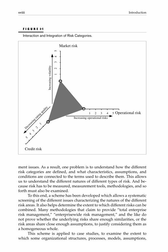
ment issues. As a result, one problem is to understand how the differentrisk categories are defined, and what characteristics, assumptions, andconditions are connected to the terms used to describe them. This allowsus to understand the different natures of different types of risk. And be-cause risk has to be measured, measurement tools, methodologies, and soforth must also be examined.

To this end, a scheme has been developed which allows a systematicscreening of the different issues characterizing the natures of the differentrisk areas. It also helps determine the extent to which different risks can becombined. Many methodologies that claim to provide “total enterpriserisk management,” “enterprisewide risk management,” and the like donot prove whether the underlying risks share enough similarities, or therisk areas share close enough assumptions, to justify considering them asa homogeneous whole.

This scheme is applied to case studies, to examine the extent towhich some organizational structures, processes, models, assumptions,

xviii Introduction

5

4

3

2

1

1

2

3

4

5

1 2 3 4 5

Credit risk

Market risk

Operational risk

Decrea

sing r

ating

quali

ty

Incr

easi

ng v

olat

ility

Increasing operational risks

F I G U R E I-1

Interaction and Integration of Risk Categories.

Gallati_fm_1p_j.qxd 2/27/03 9:15 AM Page xviii

methodologies, and so forth have proved applicable, and the extent of theserious financial, reputational, and sometimes existential damages thathave resulted when they have not.

APPROACH

This work focuses on the level above the financial instruments and is in-tended to add value at the organization, transaction, and process levels soas to increase the store of knowledge already accumulated. The pricing ofinstruments and the valuation of portfolios are not the primary objects ofthis book. Substantial knowledge has already been developed in this areaand is in continuous development. Risk management at the instrumentlevel is an essential basis for understanding how to make an institution’srisk management structures, processes, and organizations efficient and effective.

This book aims to develop a scheme or structure to screen and com-pare the different risk areas. This scheme must be structured in such a way that it considers the appropriateness and usefulness of the differentmethodologies, assumptions, and conditions for economic and regulatorypurposes.

The objectives of this book are as follows:• Define the main terms used for the setup of the scheme, such as

systemic, market, credit, and operational risk.• Review the methodologies, assumptions, and conditions

connected to these terms.• Structure the characteristics of the different risk areas in such a

way that the screening of these risk areas allows comparison ofthe different risk areas for economic and regulatory purposes.

In a subsequent step, this scheme is applied to a selection of casestudies. These are mainly publicized banking failures from the past decadeor so. The structured analysis of these relevant case studies should demon-strate the major causes and effects of each loss and the extent to which riskcontrol measures were or were not appropriate and effective.

The objectives of the case study analyses are as follows:• Highlight past loss experiences.• Detail previous losses in terms of systemic, market, credit, and

operational risks.• Highlight the impact of the losses.• Provide practical assistance in the development of improved risk

management through knowledge transfer and managementinformation.

• Generate future risk management indicators to mitigate thepotential likelihood of such disasters.

Introduction xix

Gallati_fm_1p_j.qxd 2/27/03 9:15 AM Page xix

C H A P T E R 1

Risk Management: A Maturing Discipline

1.1 BACKGROUND

The entire history of human society is a chronology of exposure to risksof all kinds and human efforts to deal with those risks. From the firstemergence of the species Homo sapiens, our ancestors practiced risk man-agement in order to survive, not only as individuals but as a species. Thesurvival instinct drove humans to avoid the risks that threatened extinc-tion and strive for security. Our actual physical existence is proof of ourancestors’ success in applying risk management strategies.

Originally, our ancestors faced the same risks as other animals: thehazardous environment, weather, starvation, and the threat of beinghunted by predators that were stronger and faster than humans. The en-vironment was one of continuous peril, with chronic hunger and danger,and we can only speculate how hard it must have been to achieve a sem-blance of security in such a threatening world.

In response to risk, our early ancestors learned to avoid dangerousareas and situations. However, their instinctive reactions to risk and theiradaptive behavior do not adequately answer our questions about how theysuccessfully managed the different risks they faced. Other hominids did notattain the ultimate goal of survival—including H. sapiens neanderthalensis,despite the fact that they were larger and stronger than modern humans.The modern humans, H. sapiens sapiens, not only survived all their relativesbut proved more resilient and excelled in adaptation and risk management.

Figure 1-1 shows the threats that humans have been exposed to overthe ages, and which probably will continue in the next century, as well. Itis obvious that these threats have shifted from the individual to society

1

Gallati_01_1p_j.qxd 2/27/03 9:11 AM Page 1


2

1800 1900 20001700Middle Ages0Stone Age

Indi

vidu

alG

roup

Nat

ion

Wor

ld

Slavery, violations of human rights

Robbery, tyranny

Hunger

Diseases, epidemics

Local wars

Life at subsistence level

Lack of work

Threats to social security

Economic underdevelopment

Wars on national level

Atomic threat

Overpopulation

Exhaustion of nonrenewable energy

Environmental destruction

F I G U R E 1-1

Development of the Threats to Individuals, Groups, Nations, and the World.


and the global community. Thousands of years ago, humans first learnedto cultivate the wild herbs, grasses, grains, and roots that they had tradi-tionally gathered. Concurrently, humans were creating the first settle-ments and domesticating wild animals. Next, humans began to grow,harvest, and stockpile grain, which helped to form the concept of owner-ship. Over time, humans learned to defend their possessions and their in-terests, to accumulate foodstuffs and other goods for the future, and tolive together in tribal and other communal settings. As wealth accumu-lated in modest increments, rules about how to live together were needed,and the first laws to govern human interaction were developed. Thus, thebeginning of civilization was launched. Walled cities, fortifications, andother measures to protect property and communities demonstrate thatwith increases in wealth came increased risk in a new form. Old forms,which had threatened humans for generations, were replaced by newthreats. Famine and pestilence were frequent crises, and the perils of na-ture destroyed what communities and individuals had built. Warfare andplundering increased the threats. As a result, our ancestors created tech-nologies, war strategies, and social and legal rules to survive.

The evolution of business risks coincides with the start of trading andcommerce. We do not know exactly when trading and commerce began,but their rise is clearly connected with the fact that society took advantageof specialization, which increased the capacity to produce and stockpilegoods for future use. Stockpiling goods acts as a cushion against misfor-tune, the perils of nature, and the ravages of war. It is very probable thatbusiness, in the form of trading and commerce, was one of the first activeefforts of society to deal with risk. Artifacts unearthed by archaeologistsprove that those early businesspeople developed techniques for dealingwith risk. Two major techniques are noteworthy and should be mentioned.

First, in 3000 B.C., the Babylonian civilization, with its extensive traderelations, exhibited a highly developed bureaucracy and trading sectorwith a monetary and legal system.

One consequence of the concept of private property was the evolu-tion of a market economy, but until the innovation of money was intro-duced, commerce was on a barter basis. There is some debate regardingthe exact moment when money was first used, but its use revolutionizedcommerce, private property, and the accumulation of wealth. It pro-vided a new means of stockpiling resources, and thus had an importantimpact on risk management. With the introduction of money as a storagemedium, wealth could be held in the form of tangible property or as anasset that could be exchanged for tangible properties. Physical assetscould be acquired even by those who did not have financial assets, pro-vided someone was willing to lend the money, which was the innovationof credit. This created risk for the lender, who was compensated bycharging interest for loans.



The legal system was the second innovation that revolutionized soci-ety. Laws or rules originated as tribal conventions, which became more for-malized over time. One of the first formal legal codes was established byHammurabi between 1792 and 1750 B.C. There were no other major legal sys-tem innovations until the beginning of the Industrial Revolution, so we canfly over the periods of the Egyptian, Greek, and Roman empires, feudalism,the rise of the merchant class, and mercantilism. The beginning of the In-dustrial Revolution was characterized by two major events. Modern capital-ism emerged after a transition period over several centuries, during whichthe conditions needed for a capitalistic market society were created. Amongthese conditions were formalized private ownership of the means of pro-duction, profit orientation, and the mechanisms of a market economy. Withexpanding industrial and economic activity, new organizational forms wereneeded to raise large amounts of capital and build production capacity. Thecorporation limited individual risk and leveraged production, distribution,and capital resources. The earliest form of shareholder organization, the jointstock company, appeared at the end of the seventeenth century. The investorspooled their funds, allowing multiple investors to share in both the profitsand risks of the enterprise. This feature was equivalent to partnerships andother joint forms and was not an innovation. But the corporation addressedrisk in a different way, by limiting the liability of the investors based on theamount invested. From a legal standpoint, a corporation is an artificial con-struct or artificial person, whose competencies and responsibilities are sepa-rate from those of the investor-owners (with exceptions).

The Industrial Revolution created new sources of risks. The applica-tion of steam power to the production process and transportation replacedold threats with the new risks that accompany advancing technologies.With the emergence of the age of information technology, inherent risksinclude business system problems, fraud, and privacy issues, which canall interrupt the day-to-day operations of a business.

Although the term risk management originated in the 1950s, HenryFayol recognized its significance earlier.1 Fayol, a leading managementauthority, was influenced by growing mass production in the UnitedStates, and the existence of giant corporations and their managementchallenges. In 1916, he structured industrial activities into six functions,including one called security, which sounds surprisingly like the conceptof risk management:

The purpose of this function is to safeguard property and persons againsttheft, fire and flood, to ward off strikes and felonies and broadly all socialdisturbances or natural disturbances liable to endanger the progress andeven the life of the business. It is the master’s eye, the watchdog of the one-man business, the police or the army in the case of the state. It is generallyspeaking all measures conferring security upon the undertaking and requi-site peace of mind upon the personnel.2

4 CHAPTER 1


Centuries ago, bandits and pirates threatened traders. Now hackersare engaged in vandalism and commit electronic larceny.

The media are full of news about the perils of human-made and nat-ural hazards. The nuclear power plant accidents at the Three Mile Islandfacility in Pennsylvania in 1979 and at Chernobyl in Ukraine in 1987 showthe new risks posed by human-made hazards and the seriousness of thesethreats. Destructive natural hazards exist as well. Hurricane Andrewcaused damages of around $22 billion; and the floods in the midwesternUnited States in 1993 and the earthquakes in California in 1993 and inKobe, Japan, in 1994 had devastating effects. In addition, terrorist activi-ties have become more dangerous over the years, as demonstrated by the1993 and 2001 bombings of the World Trade Center in New York, and the1995 bombing of the Murrah Federal Building in Oklahoma City.

A review of the past along with an assessment of the growing arrayof risks shows that the impact of risks (in terms of financial losses) has in-creased. This is not only a consequence of the increased numbers of riskswe are confronted with; the severity and frequency of disasters has in-creased as well. The financial losses from natural perils, such as floods,forest fires, and earthquakes, are not only a function of the number ofevents, as natural disasters occur with a certain average frequency as inthe past. However, each catastrophe seems to be worse than the one thatcame before it. The ultimate reason is obvious: as more and more peoplelive close together, business has become more capital intensive, and ourinfrastructure is more vulnerable and capital intensive as well. With theincreased growth of capital investment in infrastructure, manufacturingcapacity, and private ownership of real estate and other goods, the risk offinancial losses increased substantially.

1.2 RISKS: A VIEW OF THE PAST DECADES

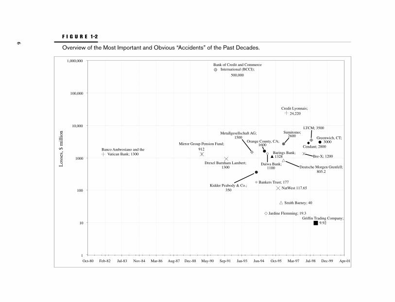
Recently, there have been a number of massive financial losses due to in-adequate risk management procedures and processes (Figure 1-2). The fail-ures of risk management in the world of finance were not primarily due tothe incorrect pricing of derivative instruments. Rather, the necessary su-pervisory oversight was inadequate. The decision makers in control of or-ganizations left them exposed to risks from derivative transactions andinstitutional money. Risk management does not primarily involve the cor-rect pricing of derivative instruments—rather, it involves the supervision,management, and control of organizational structures and processes that dealwith derivatives and other instruments.

Many cases in which managers focused on the correct pricing of financial instruments and neglected the other dimensions show the dramatic consequences of this one-dimensional understanding of riskmanagement. In Switzerland, the pension fund scheme of Landis & Gyr



6

Bankers Trust; 177

Jardine Flemming; 19.3

NatWest 117.65

Smith Barney; 40

24,220

3000

Griffin Trading Company;9.92

1300

500,000

912

1500

Kidder Peabody & Co.;350

Orange County, CA;

Bank of Credit and CommerceInternational (BCCI);

Banco Ambrosiano and theVatican Bank; 1300

Los

ses,

$ m

illio

n

Mirror Group Pension Fund;

Drexel Burnham Lambert;

Credit Lyonnais;

Metallgesellschaft AG;

1600

Barings Bank;1328

Daiwa Bank; 1100

Sumitomo;LTCM; 3500

2600

Deutsche Morgen Grenfell;805.2

Bre-X; 1200

Cendant; 2800

Greenwich, CT;

1

10

100

1000

10,000

100,000

1,000,000

Oct-80 Feb-82 Jul-83 Nov-84 Mar-86 Aug-87 Dec-88 May-90 Sep-91 Jan-93 Jun-94 Oct-95 Mar-97 Jul-98 Dec-99 Apr-01

F I G U R E 1-2

Overview of the Most Important and Obvious “Accidents” of the Past Decades.


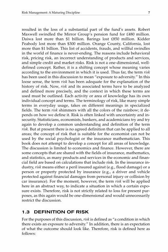
resulted in the loss of a substantial part of the fund’s assets. RobertMaxwell swindled the Mirror Group’s pension fund for £480 million.Daiwa lost more than $1 billion. Barings lost £850 million. KidderPeabody lost more than $300 million. Orange County, California, lostmore than $1 billion. This list of accidents, frauds, and willful swindlesin the world of finance is never-ending. The reasons include behavioralrisk, pricing risk, an incorrect understanding of products and services,and simple credit and market risks. Risk is not a one-dimensional, well-defined concept. Rather, it is a shifting concept whose meaning variesaccording to the environment in which it is used. Thus far, the term riskhas been used in this discussion to mean “exposure to adversity.” In thisloose sense, the term risk has been adequate for the explanation of thehistory of risk. Now, risk and its associated terms have to be analyzedand defined more precisely, and the context in which these terms areused must be outlined. Each activity or area of knowledge has its ownindividual concept and terms. The terminology of risk, like many simpleterms in everyday usage, takes on different meanings in specializedfields. The term risk shimmers with all the colors of the rainbow; it de-pends on how we define it. Risk is often linked with uncertainty and in-security. Statisticians, economists, bankers, and academicians try and tryagain to develop a common understanding and definition of the termrisk. But at present there is no agreed definition that can be applied to allareas; the concept of risk that is suitable for the economist can not beused by the social psychologist or the insurance mathematician. Thisbook does not attempt to develop a concept for all areas of knowledge.The discussion is limited to economics and finance. However, there aresome concepts that are shared with the fields of insurance, mathematics,and statistics, as many products and services in the economic and finan-cial field are based on calculations that include risk. In the insurance in-dustry, risk means either a peril insured against (e.g., flood damage) or aperson or property protected by insurance (e.g., a driver and vehicleprotected against financial damages from personal injury or collision bycar insurance). For the moment, however, the term risk will be appliedhere in an abstract way, to indicate a situation in which a certain expo-sure exists. Therefore, risk is not strictly related to loss for present pur-poses, as this again would be one-dimensional and would unnecessarilyrestrict the discussion.

1.3 DEFINITION OF RISK

For the purposes of this discussion, risk is defined as “a condition in whichthere exists an exposure to adversity.” In addition, there is an expectationof what the outcome should look like. Therefore, risk is defined here asfollows:



risk A condition in which there exists a possibility of deviation from a desiredoutcome that is expected or hoped for.

Other definitions include the restriction that risk is based on real-world events, including a combination of circumstances in the external en-vironment. We do not agree with this limitation. Potential risks that mightoccur in the future are excluded. In addition, we do not limit the range ofrisk to circumstances in the external environment. Many crises in theeconomy and the financial services industry happen because of problemswithin organizations. These often have to do with problems in the humanresource area, which belong in the realm of the behavioral sciences.

The term risk is linked to the possibility of deviation. This means thatthe possibility of risk can be expressed as a probability, ranging from 0 to100 percent. Therefore, the probability is neither impossible nor definite.This definition does not require that the probability be quantified, onlythat it must exist. The degree of risk may not be measurable, for whateverreason, but the probability of the adverse outcome must be between 0 and100 percent.

Another key element of the definition is the “deviation from a de-sired outcome that is expected or hoped for.” The definition does not sayhow such an undesirable deviation is defined. There are many ways ofbuilding expectations. By projecting historical data into the future, webuild expectations. This pattern of behavior can be observed in our every-day lives. Another way of building expectations is to forecast by using in-formation directed toward the future, not by looking back. The definitionof expectations is absolutely key in the concept of risk, as it is used to definethe benchmark. Any misconception of the expectations will distort themeasurement of risk substantially. This issue is discussed in full in the au-diting and consulting literature, which analyzes the problem of risk andcontrol in great depth.3

Many definitions of risk include the term adverse deviation to expressthe negative dimension of the expected or hoped-for outcome. We do notagree with this limitation, which implies that risk exists only with adversedeviations, which must be negative and thus are linked to losses. Such arestriction would implicitly exclude any positive connotations from theconcept of risk. We believe that risk has two sides, which both have to beincluded in the definition, and that risk itself has no dimension, negativeor positive.

1.4 RELATED TERMS AND DIFFERENTIATION

Frequently, terms such as peril, hazard, danger, and jeopardy are used inter-changeably with each other and with the term risk. But to be more preciseabout risk, it is useful to distinguish these terms:

8 CHAPTER 1


• Peril. A peril creates the potential for loss. Perils include floods,fire, hail, and so forth. Peril is a common term to define a dangerresulting from a natural phenomenon. Each of the eventsmentioned is a potential cause of loss.

• Hazard. A hazard is a condition that may create or increase thechance of a loss arising from a given peril. It is possible forsomething to be both a peril and a hazard at the same time. Forinstance, a damaged brake rotor on a car is a peril that causes aneconomic loss (the brake has to be repaired, causing financialloss). It is also a hazard that increases the likelihood of loss fromthe peril of a car accident that causes premature death.

Hazards can be classified into the following four main categories:

• Physical hazard. This type of hazard involves the physicalproperties that influence the chances of loss from various perils.

• Moral hazard. This type of hazard involves the character ofpersons involved in the situation, which might increase thelikelihood of a loss. One example of a moral hazard is the dishonestbehavior of a person who commits fraud by intentionallydamaging property in order to collect an insurance payment. Thisdishonest behavior results in a loss to the insurance company.

• Morale hazard. This type of hazard involves a careless attitudetoward the occurrence of losses. An insured person ororganization, knowing that the insurance company will bear thebrunt of any loss, may exercise less care than if forced to bear anyloss alone, and may thereby cause a condition of morale hazard,resulting in a loss to the insurance company. This hazard shouldnot be confused with moral hazard, as it requires neitherintentional behavior nor criminal tendencies.

• Legal hazard. This type of hazard involves an increase in theseverity and frequency of losses (legal costs, compensationpayments, etc.) that arises from regulatory and legal requirementsenacted by legislatures and self-regulating bodies and interpretedand enforced by the courts. Legal hazards flourish in jurisdictionsin which legal doctrines favor a plaintiff, because this represents ahazard to persons or organizations that may be sued. The Americanand European systems of jurisprudence are quite different. In theAmerican system, it is much easier to go to court, and producers ofgoods and services thus face an almost unlimited legal exposure topotential lawsuits. The European courts have placed higher hurdlesin the path of those who might take legal action against anotherparty. In addition, “commonsense” standards of what is actionableare different in Europe and the United States.



For a risk manager, the legal and criminal hazards are especially im-portant. Legal and regulatory hazards arise out of statutes and court deci-sions. The hazard varies from one jurisdiction to another, which meansglobal companies must watch legal and regulatory developments carefully.

1.5 DEGREE OF RISK

Risk itself does not say anything about the dimension of measurement.How can we express that a certain event or condition carries more or lessrisk than another? Most definitions link the degree of risk with the likeli-hood of occurrence. We intuitively consider events with a higher likeli-hood of occurrence to be riskier than those with a lower likelihood. Thisintuitive perception fits well with our definition of the term risk. Most def-initions regard a higher likelihood of loss to be riskier than a lower likeli-hood. We do not agree, as this view is already affected by the insuranceindustry’s definition of risk. If risk is defined as the possibility of a devia-tion from a desired outcome that is expected or hoped for, the degree ofrisk is expressed by the likelihood of deviation from the desired outcome.

Thus far we have not included the size of potential loss or profit inour analysis. We say that a situation carries more or less risk, and mean aswell the value impact of the deviation. The expected value of a loss orprofit in a given situation is the likelihood of the deviation multiplied bythe amount of the potential loss or profit. If the money at risk is $100 andthe likelihood of a loss is 10 percent, the expected value of the loss is $10.If the money at risk is $50 and the likelihood of a loss is 20 percent, the ex-pected value of the loss is still $10. The same calculation applies to a profitsituation. This separation of likelihood and value impact is very impor-tant, but we do not always consider this when we talk about more or lessrisk. Later we will see how the separation of likelihood and impact canhelp us analyze processes, structures, and instruments to create an overallview of organizational risk.

Frequently, persons who sit on supervisory committees (e.g., boardmembers and trustees of endowment institutions and other organiza-tions) have to make decisions with long-ranging financial impact but haveinadequate backgrounds and training to do so. Organizational structuresand processes are rarely set up to support risk management, as thesestructures are usually adopted from the operational areas. But with in-creased staff turnover, higher production volumes, expansion into newmarkets, and so forth, the control structures and processes are rarelyadapted and developed to match the changing situation.

New problems challenge management, as the existing controlprocesses and reporting lines no longer provide alerts and appropriate in-formation to protect the firm from serious damage or bankruptcy, as wasthe case with Barings or Yamaichy.

10 CHAPTER 1


Banks and other regulated financial institutions have been forced bygovernment regulations and industry self-regulating bodies to developthe culture, infrastructure, and organizational processes and structures foradequate risk management. Risk management has become a nondelegablepart of top management’s function and thus a nondelegable responsibilityand liability. Driven by law, the financial sector has developed over thepast years strategies, culture, and considerable technical and managementknow-how relating to risk management, which represents a competitiveadvantage against the manufacturing and insurance sectors.

1.6 RISK MANAGEMENT: A MULTILAYERED TERM

1.6.1 Background

As previously discussed, risk management is a shifting concept that hashad different definitions and interpretations. Risk management is basi-cally a scientific approach to the problem of managing the pure risks facedby individuals and institutions. The concept of risk management evolvedfrom corporate insurance management and has as its focal point the pos-sibility of accidental losses to the assets and income of the organization.Those who carry the responsibility for risk management (among whomthe insurance case is only one example) are called risk managers. The termrisk management is a recent creation, but the actual practice of risk man-agement is as old as civilization itself. The following is the definition ofrisk management as used used throughout this work:

risk management In a broad sense, the process of protecting one’s person or or-ganization intact in terms of assets and income. In the narrow sense, it is the mana-gerial function of business, using a scientific approach to dealing with risk. As such,it is based on a distinct philosophy and follows a well-defined sequence of steps.

1.6.2 History of Modern Risk Management

Risk management is an evolving concept and has been used in the sense de-fined here since the dawn of human society. As previously mentioned, riskmanagement has its roots in the corporate insurance industry. The earliestinsurance managers were employed at the turn of the twentieth century bythe first giant companies, the railroads and steel manufacturers. As capitalinvestment in other industries grew, insurance contracts became an increas-ingly significant line item in the budgets of firms in those industries, as well.

It would be mistaken to say that risk management evolved naturallyfrom the purchase of insurance by corporations. The emergence of riskmanagement as an independent approach signaled a dramatic, revolu-



tionary shift in philosophy and methodology, occurring when attitudestoward various insurance approaches shifted. One of the earliest refer-ences to the risk management concept in literature appeared in 1956 in theHarvard Business Review.4 In this article, Russell Gallagher proposed a rev-olutionary idea, for the time, that someone within the organization shouldbe responsible for managing the organization’s pure risk:

The aim of this article is to outline the most important principles of a work-able program for “risk management”—so far so it must be conceived, evento the extent of putting it under one executive, who in a large companymight be a full-time “risk manager.”

Within the insurance industry, managers had always considered in-surance to be the standard approach to dealing with risk. Though insurancemanagement included approaches and techniques other than insurance(such as noninsurance, retention, and loss prevention and control), these ap-proaches had been considered primarily as alternatives to insurance.

But in the current understanding, risk management began in the early1950s. The change in attitude and philosophy and the shift to the risk man-agement philosophy had to await management science, with its emphasis oncost-benefit analysis, expected value, and a scientific approach to decisionmaking under uncertainty. The development from insurance managementto risk management occurred over a period of time and paralleled the evolu-tion of the academic discipline of risk management (Figure 1-3). Operationsresearch seems to have originated during World War II, when scientists wereengaged in solving logistical problems, developing methodologies for deci-phering unknown codes, and assisting in other aspects of military opera-tions. It appears that in the industry and in the academic discipline thedevelopment happened simultaneously, but without question the academicdiscipline produced valuable approaches, methodologies, and models thatsupported the further development of risk management in the industry.New courses such as operations research and management science empha-size the shift in focus from a descriptive to a normative decision theory.

Markowitz was the first financial theorist to explicitly include risk inthe portfolio and diversification discussion.5 He linked terms such as returnand utility with the concept of risk. Combining approaches from operationsresearch and mathematics with his new portfolio theory, he built the basisfor later developments in finance. This approach became the modern portfo-lio theory, and was followed by other developments, such as Fischer Black’soption-pricing theory, which is considered the foundation of the deriva-tives industry. In the early 1970s, Black and Scholes made a breakthroughby deriving a differential equation which must be satisfied by the price ofany derivative instrument dependent on a nondividend stock.6 This ap-proach has been developed further and is one of the driving factors for theactual financial engineering of structured products.

12 CHAPTER 1


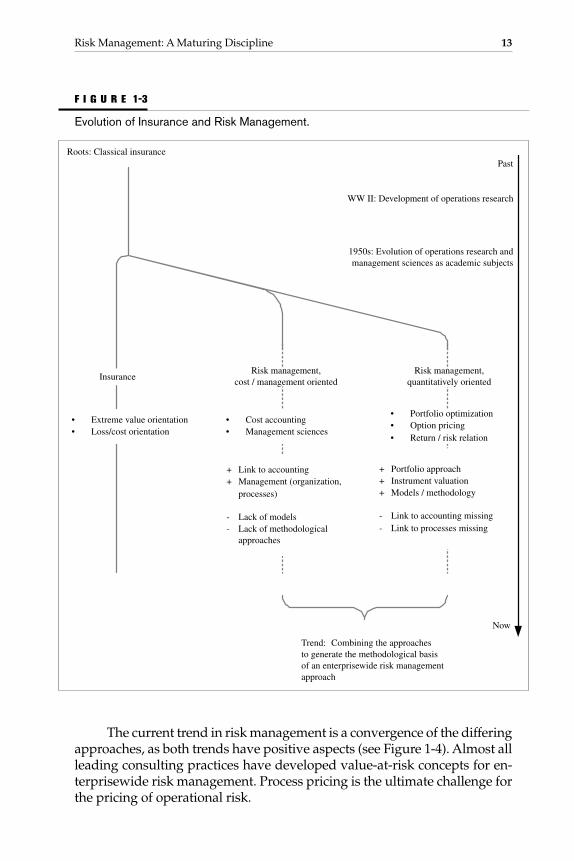
The current trend in risk management is a convergence of the differingapproaches, as both trends have positive aspects (see Figure 1-4). Almost allleading consulting practices have developed value-at-risk concepts for en-terprisewide risk management. Process pricing is the ultimate challenge forthe pricing of operational risk.


Risk management,cost / management oriented

• Portfolio optimization• Option pricing• Return / risk relation

+ Portfolio approach+ Instrument valuation+ Models / methodology

- Link to accounting missing- Link to processes missing

+ Link to accounting+ Management (organization,

processes)

- Lack of models- Lack of methodological

approaches

• Cost accounting• Management sciences

• Extreme value orientation• Loss/cost orientation

Insurance

Trend: Combining the approachesto generate the methodological basisof an enterprisewide risk managementapproach

Roots: Classical insurancePast

Now

WW II: Development of operations research

1950s: Evolution of operations research andmanagement sciences as academic subjects

Risk management,quantitatively oriented

F I G U R E 1-3

Evolution of Insurance and Risk Management.


14

Iden

tific

atio

nof

ris

k

Mea

sure

men

tof

ris

k

Con

trol

of

risk

Lin

king

ris

kan

d re

turn

Cap

ital

allo

catio

npr

oces

s

Cap

ital

allo

catio

nte

chni

ques

Val

ue-b

ased

stra

tegy

Max

imiz

edea

rnin

gspo

tent

ial

Ear

ning

sst

abili

ty

Prot

ectio

nag

ains

tun

fors

een

loss

es

Stra

tegi

c ad

vant

age

Cre

dit r

isk

Mar

ket r

isk

Shareholder value objective

Ris

k m

anag

emen

t so

phis

tica

tion

Ope

ratio

nal r

isk

FI

GU

RE

1-4

Dev

elop

men

t Lev

els

of D

iffer

ent R

isk

Cat

egor

ies.


1.6.3 Related Approaches

1.6.3.1 Total Risk ManagementTotal risk management, enterprisewide risk management, integrated risk man-agement, and other terms are used for approaches that implementfirmwide concepts including measurement and aggregation techniquesfor market, credit, and operational risks. This book uses the following def-inition for total risk management, based on the understanding in the mar-ket regarding the concept:

total risk management The development and implementation of an enter-prisewide risk management system that spans markets, products, and processesand requires the successful integration of analytics, management, and technology.

The following paragraphs highlight some concepts developed byconsulting and auditing companies. Enterprise risk management, as devel-oped by Ernst & Young, emphasizes corporate governance as a key elementof a firmwide risk management solution. Boards that implement leading-edge corporate governance practices stimulate chief executives to sponsorimplementation of risk management programs that align with their busi-nesses. In fulfilling their risk oversight duties, board members request reg-ular updates regarding the key risks across the organization and theprocesses in place to manage them. Given these new practices, boards areincreasingly turning to the discipline of enterprise risk management as ameans of meeting their fiduciary obligations. As a result, pioneering or-ganizations and their boards are initiating enterprisewide risk manage-ment programs designed to provide collective risk knowledge for effectivedecision making and advocating the alignment of management processeswith these risks. These organizations have recognized the advantages of:

• Achieving strategic objectives and improving financialperformance by managing risks that have the largest potentialimpact

• Assessing risk in the aggregate to minimize surprises and reduceearnings fluctuations

• Fostering better decision making by establishing a commonunderstanding of accepted risk levels and consistent monitoringof risks across business units

• Improving corporate governance with better risk managementand reporting processes, thereby fulfilling stakeholderresponsibilities and ensuring compliance with regulatoryrequirements

At present, many risk management programs attempt to provide alevel of assurance that the most significant risks are identified and man-



aged. However, they frequently fall short in aggregating and evaluatingthose risks across the enterprise from a strategic perspective. Effective en-terprise risk management represents a sophisticated, full-fledged man-agement discipline that links risk to shareholder value and correlates withthe complexity of the organization and the dynamic environments inwhich it operates (Figure 1-5).

Once an organization has transformed its risk management capabil-ities, it will be in a position to promote its success through an effective, in-tegrated risk management process. Ernst & Young’s point of view is thateffective enterprise risk management includes the following points (seeFigure 1-6):7

• A culture that embraces a common understanding and vision ofenterprise risk management

• A risk strategy that formalizes enterprise risk management andstrategically embeds risk thinking within the enterprise

16 CHAPTER 1

F I G U R E 1-5

Evolving Trends and the Development of an Integrated Risk Framework to Supportthe Increasing Gap Between Business Opportunities and Risk Management Capa-bilities. (Source: Ernst & Young, Enterprise Risk Management, Ernst & Young LLP,2000. Copyright © 2000 by Ernst & Young LLP; reprinted with permission of Ernst& Young LLP.)


• An evolved governance practice that champions an effectiveenterprisewide risk management system

• Competent and integrated risk management capabilities foreffective risk identification, assessment, and management

Coopers & Lybrand has developed its own version of an enter-prisewide risk management solution in the form of generally accepted riskprinciples (GARP).8 The GARP approach seeks to distil and codify majorprinciples for managing and controlling risk from the guidance issued todate by practitioners, regulators, and other advisors. The framework usesthe experience and expertise of all parties involved in its development toexpand these principles so as to establish a comprehensive frameworkwithin which each firm can manage its risks and through which regulatorscan assess the adequacy of risk management in place. It presents a set ofprinciples for the management of risk by firms, and for the maintenance ofa proper internal control framework, going further than the mere assess-ment of the algorithms within risk management models. It covers such


assuredsupported

and

stakeholder

communications

functio

ns

technology

risk management

capabilityriskmana

gement

process

riskstrategy

cultureand

governance

embedded

valu

eba

sed

shar

ehol

der

reviewed

F I G U R E 1-6

Enterprise Risk Management Point of View. (Source: Ernst & Young LLP, a mem-ber of Ernst & Young Global. Copyright © 2002 by Ernst & Young LLP; reprintedwith permission of Ernst & Young LLP.)


matters as the organization of the firm, the operation of its overall controlframework, the means and principles of risk measurement and reporting,and the systems themselves. The approach is based around principles, eachof which is supported by relevant details. The extent of the detail variesdepending on the principle concerned. In all cases, the guidance providedis based on the assumption that the level of trading in a firm is likely togive rise to material risks. In certain cases an indication of alternative ac-ceptable practices is given.

KPMG has developed a risk management approach based on theshareholder value concept, in which the value of an organization is notsolely dependent on market risks, such as interest or exchange rate fluc-tuations. It is much more important to study all types of risks. Thismeans that macroeconomic or microeconomic risks, on both the strategicand operational levels, have to be analyzed and considered in relation toevery single decision. An organization can seize a chance for lasting andlong-term success only if all risks are defined and considered in its overalldecision-making process as well as in that of its individual businessunits. KPMG assumes (as do other leading companies) that the key fac-tor for a total risk management approach is the phase of risk identifica-tion, which forms the basis for risk evaluation, risk management, andcontrol. Figure 1-7 shows the Risk Reference Matrix, KPMG’s systematicand integrated approach to the identification of risk across all areas ofthe business.9 This is a high-level overview, which can be further brokendown into details.

Many other approaches from leading consulting and auditing prac-tices could be mentioned. They all assume that they have a frameworkthat contains all the risks that must be identified and measured to get theoverall risk management.

Figure 1-8 shows a risk map that covers many different risk areas,from a high-level to low-level view. From an analytical standpoint, it looksconsistent and comprehensive, covering all risks in an extended frame-work. The allocation of individual risks may be arbitrary, depending onwhat concept is used. But the combination and complexity of all risks,their conditions and assumptions, might make it difficult to identify andmeasure the risk for an enterprisewide setup.

In practice, significant problems often occur at this stage. A system-atic and consistent procedure to identify risk across all areas of the busi-ness, adhering to an integrated concept, is essential to this first sequenceof the risk management process. But this integrated concept is, in certainregards, a matter of wishful thinking. The definition of certain individualrisks—for example, development, distribution, and technology risks—isnot overly problematic. The concepts span the complete range of riskterms. But in many cases the categorization and definition of some termsare ambiguous. One example is the term liquidity. Liquidity can be seen as

18 CHAPTER 1


part of market and credit risks, but it also affects systemic risk. The totalrisk management concept appears to be complete, consistent, and ade-quate. But this interpretation is too optimistic, as some of the concepts stilllack major elements and assumptions.

In an overall approach, the interaction between individual risks, aswell as the definition of the weighting factors between the risk trees thatmust be attached to this correlation, creates serious difficulties. Portfoliotheory tells us that correlation between the individual risk elements rep-


TOTAL

RISK

BusinessEnvironment Risk

Activity Risk

MacroeconomicRisk Factors

MicroeconomicRisk Factors

Cultural-LevelRisks

Strategic-LevelRisks

Operational-LevelRisks

InternationalStability Risk

National StabilityRisk

Outside RiskFactors

Financial MarketRisks

Development &Production Risks

Customer-FacingRisks

OrganizationalPolicy Risks

General Industry-Related Risks

Business PolicyRisks

Business ValueRisks

Ethical ValueRisks

Local IndustrialSector Risks

Support ServiceRisks

F I G U R E 1-7

KPMG Risk Reference Matrix. (Source: Cristoph Auckenthaler and Jürg Gabathuler,Gedanken zum Konzept eines Total Enterprise Wide Risk Management (TERM), Zurich:University of Zurich, 1997, 9, fig. 2.)


20

Market risk

Legal

Compliance

Regulatory

Human resources

Management direction anddecision making

Accounting Taxation

External physicalevents

Product / servicedevelopment

Controlframework

Suppliers

Communication / relationshipmanagement

Corporate strategy /direction

SupportServices

Internal physicalevents

Processmanagement /

design

Productselling /

distribution

Systemic risk

Credit risk

Strategic / management risk

Financial riskOperational riskSystemic risk

F I G U R E 1-8

Risk Map of a Total Risk Management Approach. (Source: Modified from KPMG.)


resents a central role in the establishment of risk definitions and strate-gies, and therefore in the risk management and hedging process (pro-vided hedging is feasible). The same is also true for the risk managementof a business (with elements such as new product risks, model risks,counterparty risks, etc.). From a practical standpoint, it is often not possi-ble to get data and calculate risk coefficients if the overall scheme of atotal risk management concept represents a widely branching system,because the number of interactions (correlations) and the required dataincrease substantially as the number of elements increases. Such ap-proaches require the combined and well-orchestrated use of question-naires, checklists, flowcharts, organization charts, analyses of yearlyfinancial statements and transactions, and inspections of the individualbusiness locations. This requires substantial expenditures and commit-ment from management.

As can be seen from the preceding descriptions of the different en-terprise risk management solutions, the major consulting firms approachthe same issues from different perspectives. Whereas KPMG and Ernst &Young have a more holistic approach, Coopers & Lybrand takes a morenormative, trading-oriented, and regulatory approach. Regardless of thedifferent approaches offered by the various auditing and consulting com-panies, a company has to adapt the approach it selects based on its ownneeds, its understanding of risk management, and the extent to which riskmanagement is an integrated part of upper management’s responsibilitiesor an independent control and oversight function.

1.6.3.2 Total Quality ManagementVirtually every activity within an organization changes the organiza-tion’s exposure to risk. It is part of a risk manager’s responsibility to ed-ucate others on the risk-creating and risk-reducing aspects of theiractivities. The recognition that risk control is everyone’s responsibilityclosely links risk control to principles of quality improvement, an ap-proach to management that has been employed with considerable suc-cess in Japan and the United States. The movement toward qualityimprovement often is known by code names and acronyms such as totalquality management (TQM) and total quality improvement (TQI). TQM wasdeveloped in Japan after World War II, with important contributionsfrom American experts. Ultimately, Japanese companies recognized thatproduction volume itself does not create competitive advantage, onlyquality and product differentiation can do so. In the context of TQM,quality is here defined as follows:10

quality The fulfillment of the agreed-upon requirements communicated by thecustomer regarding products, services, and delivery performance. Quality ismeasured by customer satisfaction.



TQM has five approaches, reflecting the different dimensions ofquality:11

• Transcendent approach. Quality is universally recognizable and isa synonym for high standards for the functionality of a product.The problem is that quality cannot be measured precisely underthis approach.

• Product-oriented approach. Differences in quality are observablecharacteristics linked to specific products. Thus, quality isprecisely measurable.

• User-oriented approach. Quality is defined by the user, dependingon the utility value.

• Process-oriented approach. The production process is the focus ofquality efforts. Quality results when product specifications andstandards are met through the use of the proper productionprocess.

• Value-oriented approach. Quality is defined through the price-product-service relationship. A quality product or service isidentified as one that provides the defined utility at an acceptableprice.

The TQM approach has four characteristics:

• Zero-error principle. Only impeccable components and perfectprocesses may be used in the production process to ensuresystematic error avoidance in the quality circle.

• Method of “why.” This is a rule of thumb: the basis of a problemcan be evaluated by asking why five times. This avoids taking thesymptoms of a problem to be the problem itself.

• Kaizen. Kaizen is a continuous process of improvement throughsystematic learning. This means turning away from the traditionaltayloristic division of labor and returning to an integratedorganization of different tasks that includes continuous training todevelop personnel’s technical and human relations skills.

• Simultaneous engineering. Simultaneous engineering demandsfeedback loops between different organizational units anddifferent processes. This requires overlapping teams and processorientation.12

Table 1-1 highlights the profiles of the total quality management andtotal risk management approaches.

Total quality management has its own very distinct terms and defi-nitions, which make it a different approach from total risk management. Itis a multidimensional client-oriented approach, in which managementtakes preventive measures to ensure that all processes, organizational en-

22 CHAPTER 1


tities, and employees focus on quality assurance and continuous improve-ment throughout the organization.

1.6.4 Approach and Risk Maps

Figures 1-9 and 1-10 present the approach and risk maps used in this book.

1.7 SYSTEMIC RISK

1.7.1 Definition

There is no uniform accepted definition of systemic risk. This book usesthe definition contained in a 1992 report of the Bank for International Set-tlement (BIS):13


T A B L E 1-1

Differences and Similarities Between Total Quality Management and Total Risk Management

Total Quality Management (TQM) Total Risk Management (TRM)

Extended, multidimensional, client- Integrated, multidimensional enterprise-oriented quality term. oriented term.

Extended client definition: clients are Internal client definition: clients areinternal and external. internal.

Preventive quality assurance policy. Preventive and product-oriented riskmanagement policy.

Quality assurance is the duty of all TRM assurance is the duty of speciallyemployees. assigned and responsible persons.

Enterprisewide quality assurance. TRM assurance within the limits and forthe risk factors to be measured accordingto the risk policy.

Systematic quality improvement with Systematic risk control within thezero-error target. defined limits.

Quality assurance is a strategic job. TRM is a strategic job.

Quality is a fundamental goal of the TRM is a fundamental goal of theenterprise. enterprise.

Productivity through quality. TRM to ensure ongoing production.

SOURCE: Hans-Jörg Bullinger, “Customer Focus: Neue Trends für eine zukunftsorientierte Unternehmungsführung,” inHans-Jörg Bullinger (ed.), “Neue Impulse für eine erfolgreiche Unternehmungsführung, 13. IAO-Arbeitstagung,” Forschungund Praxis, Band 43, Heidelberg u.a., 1994.


24 CHAPTER 1

Model Risk

Market Risk

Credit Risk

Operational Risk

Systemic Risk

Current Exposure

Potential Exposure

Cumulation Risk

Counterparty Risk

Direct Credit Risk

Credit EquivalentExposure

Diversification Risk

Credit Risk Exposure

RegulatoryMechanisms

Capital Adequacy

Risk Disclosure

Regulatory Constraints

Model Risk

Equity Risk

Interest Rate Risk

Currency Risk

Capital Adequacy

Risk Disclosure


Model Risk

Commodity Risk

Model Risk

Equity Price Risk

Model Risk

Yield Curve Risk Basis / Spread Risk

Product Risk

Product Risk

"Greeks"

Dividends

"Greeks"

Prepayment

Model Risk

Commodity CurveRisk

Basis / Spread Risk

"Greeks"

Model Risk

Fx Curve Risk Basis / Spread Risk

"Greeks"

Liquidity Risk Model Risk

Rating

Customer / TransactionRisks

Marketing Risks

Sales Risks

Disclosures

Product / MarketCombination

Distribution

Order Capture &Confirmation

Controlling

Internal Audit

Legal & Compliance

Business Control

Logistics

Support Service Risks

Accounting

HR

IT / Technology


Risk Disclosure


Market EfficiencyMarket Liquidity

InformationTransparency

Market Access /Hurdles

International / NationalStability Risks Economy

Legal System

Political Stability

Market Risk Factors


F I G U R E 1-9

Risk Categorization Used as an Integrative Framework in This Book.


25

PortfolioManagement

Resarch Compliance Trade ManagementTools

Order Routing Trade ExecutionTrade

ConfirmationSettlement andReconciliation

Custody orSecurities Lending Compliance

PortfolioAccounting

Market Risk Market Risk

Credit Risk Credit Risk

Legal /Regulatory

OperationalRisk

Market Risk

OperationalRisk

OperationalRisk

Systemic Risk

OperationalRisk

OperationalRisk

OperationalRisk

OperationalRisk

Legal /Regulatory

Pretrade Trade Posttrade

Market Risk

Credit Risk

During the phases of research, tactical or strategic asset allocation, and selection of instruments, there is an inherent risk of misjudgment or faulty estimation. Therefore, timing, instrument selection, and rating considerations have a market and credit component.

Compliance has to take into account all client restrictions, internal directives, and regulatory constraints affected by the intended transaction. Capital adequacy, suitability to the client's account, and so forth, also must be considered.

From the moment the trade is entered into the system until the final transaction is entered in the portfolio accounting and custody or securities lending systems, systems are crucial and have inherent risks.

During the trade execution phase, the trading desk has directed exposure to system risk. Until final settlement, the trade amount is exposed to disruption in the system, which could disturb correct trade confirmation and settlement.

From the moment of execution until settlement, the books are exposed to changes in the market risk factors. They are also exposed to changes in spread risk (i.e., credit risk).

Market risk during the trade execution is especially high, as the market price or model pricing might give the wrong information (e.g., the market could be illiquid, or the models might not fit the instruments).

Compliance can be considered the last stop before the transaction is complete. There is the opportunity to review whether the transaction has been executed and settled correctly.

F I G U R E 1-10

Example of Transaction Breakdown, Process-Oriented Flow of Different Risk Categories Involved.


systemic risk The risk that a disruption (at a firm, in a market segment, to a set-tlement system, etc.) causes widespread difficulties at other firms, in other marketsegments, or in the financial system as a whole.

In this definition, systemic risk is based on a shock or disruption originatingeither within or outside the financial system that triggers disruptions toother market participants and mechanisms. Such a risk thereby substan-tially impairs credit allocation, payments, or the pricing of financial assets.While many would argue that no shock would be sufficient to cause a totalbreakdown of the financial system, there is little doubt that shocks of sub-stantial magnitude could occur, and that their rapid propagation throughthe system could cause a serious system disruption, sufficient to threaten thecontinued operation of major financial institutions, exchanges, or settlementsystems, or result in the need for supervisory agencies to step in rapidly.

1.7.2 Causes of Systemic Risk

Under the BIS definition, one should consider not only the steps takenwithin the institution to guard against a major internal breakdown. Oneshould also consider those features of the global financial marketplaceand current approaches to risk management and supervision that couldadversely affect the institution’s ability to react quickly and appropriatelyto a shock or disturbance elsewhere.

Recent developments in the financial market have produced a broadrange of highly developed pricing models. Shareholder value, which is oftenmistakenly thought of as the generation of higher return on equity, leads fi-nancial institutions to reduce the proprietary capital used for activities that in-crease the profitability of equity capital. The financial institution reduces theequity capital to the bare regulatory minimum with the result that less and lesscapital supports the expanded trading activities, because the shareholdervalue concept has nothing to do with capital support. This trend is quitedangerous, as less and less capital serves as security capital in the return-generationprocessformoreandmorerisk,withoutgeneratingcommensuratereturns, and this trend alone promotes systemic risks. The development of aninternationally linked settlement system has progressed significantly; never-theless, there are still other factors that create systemic risk.

1.7.3 Factors That Support Systemic Risk

The following factors support systemic risk, based on empirical experi-ence from previous crises or near-misses in the market:

• Economic implications. Our understanding of the relationshipbetween the financial markets and the real state of the economy is

26 CHAPTER 1


questionable. The pricing of individual positions or positions for aportfolio can be done with any desired precision. The economicimplications of the created models are often overlooked. It is notalways a simple matter to understand the basic economicassumptions and parameters of complex mathematical models.This is one of the biggest systemic risks and a possible reason forthe irritating, erratic movements of the markets. The participants—especially the “rocket scientists,” highly intelligent but with anarrow horizon—do not understand the impact of coordinationand feedback loops among the many individual decisions on thefinancial markets, especially concerning derivative constructs.

• Liquidity. Pricing models work under the ideal assumption thatmarkets are liquid. Even worst-case scenarios and stress testing ofmarket situations assume liquid markets. Valuation models arestill hedge and arbitrage models, and are always based on theassumptions that positions can be liquidated and cash positionscan be adjusted. With illiquid markets, strategy changes orposition liquidation are difficult and sometimes impossible. Sucha situation might cause a domino effect—an institution trying toliquidate positions in an illiquid market experiences cashproblems, which causes the market to react negatively, sweepingaway other institutions. The LTCM case is a typical example ofthis kind of systemic risk exposure (see case study in Chapter 6).

It is important to distinguish between liquidity risk as part of sys-temic risk and liquidity risk as part of market and credit risk. Market liq-uidity risk as part of systemic risk relates to the market itself, not to thepricing of individual positions.

The over-the-counter (OTC) market is a very attractive market for fi-nancial institutions, as the margins in this market are higher than ontraded exchanges. The volume in the OTC market is enormous, but non-transparent. Transactions are not subject to the same clearing, settlement,and margin requirements as on traded exchanges. The risk of the OTCmarket, then, is that it is nontransparent, noninstitutionalized, and almostunregulated. Surprises may appear out of nowhere, and they may causequick market reactions, disrupting the financial system with feedbackloops and affecting financial institutions.

1.7.4 Regulatory Mechanisms for Risk Management

The regulatory bodies have recognized the need for adequate risk meas-urement and management techniques and approaches. The toolbox of theregulators is not limited to quantitative models, as many accidents and



near-misses have highlighted the need for transparency and disclosure ofmarket, credit, and operational risk information. A well-informed investoris well positioned to adjust the price based on available information, re-flecting the expected risk premium for the entity being invested in.

Minimum disclosure requirements, risk management and controlguidance through local supervisors, cross-border coordination of localregulators, and shared control of supranational organizations are some ofthe options regulators can select to keep systemic risk under control. Thefollowing topics highlight the focus of regulations recently published byBIS, and also indicate the mindset of the regulators, based on some recentaccidents:

• Enhancing Bank Transparency, September 1998. Public disclosureand supervisory information that promote safety and soundnessin banking systems.14

• Supervisory Information Framework for Derivatives and TradingActivities, September 1998. Joint Report by the Basel Committeeon Banking Supervision and the Technical Committee of theInternational Organization of Securities Commissions (IOSCO).15

• Framework for Internal Control Systems in Banking Organisations,September 1998.16

• Essential Elements of a Statement of Cooperation Between BankingSupervisors, May, 2001. Framework for cross-border cooperationamong different local regulators.17

• Conducting a Supervisory Self-Assessment: Practical Application,April 2001; The Relationship Between Banking Supervisors and Banks’External Auditors, February 2001. Guidelines for local regulatorsto assess their own supervisory abilities and the nationalsupervisory frameworks.18

• Best Practices for Credit Risk Disclosure, September 2000; IndustryViews on Credit Risk Mitigation, January 2000; Range of Practice inBanks’ Internal Ratings Systems, January 2000. Reviews of currentbest practices for credit risk disclosures, which became part of thenew capital adequacy framework to increase the quality level ofdisclosed information and generate peer pressure.19

• Review of Issues Relating to Highly Leveraged Institutions, March2001; Banks’ Interactions with Highly Leveraged Institutions, January2000. Reviews and recommendations regarding banks’ exposureand transactions with highly leveraged institutions, based on theLTCM crisis of September 1998.20

The approach of the BIS regulations is clearly a combination of thevarious measures available to the supervisory organizations, designed toavoid systemic risks and protect clients through increased disclosure and

28 CHAPTER 1


transparency and more precise calculation of the capital needed to sup-port risks.

None of the previously mentioned approaches would achieve theseobjectives on their own. Thus, the new capital adequacy approach inte-grates the different risk categories and the different supervisory tools inthe form of capital adequacy calculation, disclosure requirements, cross-border cooperation among supervisors, and the like.

1.8 SUMMARY

Risk management is not a new function or gadget in the financial industry.However, based on recent events, regulators and the media have increas-ingly scrutinized risk management practices and techniques. A closer lookat some of the accidents makes it apparent that managers, regulators, andinvestors have partially lost control of risk management, overestimatedtheir own capabilities and capacities, and brought companies and entiremarkets to the edge of the abyss.

For well over 100 years, farmers, for example, have engaged in riskmanagement as they have sought to hedge their crops against price fluc-tuations in commodity markets. Their preferred strategy has been to sellshort some or all of their anticipated crops before harvest time to anotherparty on what are called futures markets. The Chicago Board of Trade(CBOT) was the first exchange to offer futures contracts. This strategyguarantees the farmer a known price for a crop, regardless of what thecommodity’s future price turns out to be when the crop is harvested. Riskmanagement along these lines makes sense for farmers for at least tworeasons. First, agricultural prices are exposed to volatility. Many of thesefarmers are not diversified and must also borrow in order to finance theircrops. Therefore, setting the future sale price now migrates the risk ofprice fluctuations.

For another example that demonstrates the same approach, considera large aluminum extraction company, owned by numerous shareholders,facing similar commodity price risk. For concreteness, consider a firm pri-marily engaged in the extraction and sale of raw aluminum on a globalbasis. Given that aluminum prices are relatively volatile and are exposedto global economic cycles, the first rationale for risk management mightseem similar to the farmer’s. However, unlike the farmer’s circumstance,this firm is owned by a large number of shareholders, who can, if theywish, greatly reduce or eliminate their risk from low aluminum pricessimply by holding a diversified portfolio that includes only a small frac-tion of assets invested in the aluminum extraction company. More gener-ally, if investors can freely trade securities in many firms, they can choosetheir exposure to volatility in aluminum prices. Indeed, in two studies,Modigliani and Miller21 showed that, in a world with no transactions costs



or taxes and with equal information, managers could not benefit theirshareholders by altering the risk profile of the firm’s cash flow. Essentially,in this situation, shareholders can already do whatever they choose at nocost; actions by managers are redundant.

Although the Modigliani and Miller studies considered the optionsof changing the firm’s risk profile only through the use of debt financing(1958),22 or the distribution (or lack thereof) of dividends (1961),23 and notthrough the use of financial derivative securities, the powerful implicationhere is the same as that outlined earlier.

However, the practical world is not without transaction costs andnot as transparent as academic assumptions would have it. Several timesover the past decades, investors and the market have been surprised bythe announcement that a company has incurred substantial losses throughspeculation, fraud, or money laundering, leaving investors with dramati-cally devalued investments or even in bankruptcy. No risk managementstrategy as proposed by Miller and Modigliani could have prevented sucha disaster, as shareholders were unable to take any action to offset or mit-igate the risks.

Regulators have become more active over the past decades and havelaunched several initiatives regarding credit, market, and operational risks,forcing financial organizations to invest in their infrastructure, processes,and knowledge bases. The objective of both management and the regula-tors is to build and enforce an integrated risk management framework.However, although the objective might be the same, the strategy is com-pletely different from the regulatory and management viewpoints, whichis why risk management has become a hot issue. Management seeks toprotect clients’ assets at the lowest possible cost by avoiding losses and byincreasing the value of the shareholders’ investment through business de-cisions that optimize the risk premium. Regulators seek to protect theclients’ assets without regard to cost, maintaining market stability and pro-tecting the financial market by excluding systemic risk.

Risk management has to serve both purposes and thus has to bestructured, built, and managed in such a way that it can answer these dif-ferent needs simultaneously. The models and approaches used in the dif-ferent risk categories must give statements about the risk exposures andallow aggregation of risk information across different risk categories. It isthe purpose of this book to look into the different models and analyze thecompatibility, assumptions, and conditions between the different modelsand risk categories.

1.9 NOTES

1. Henri Fayol, General and Industrial Management, New York: Pitman, 1949.English translation of book originally published in French in 1916.

30 CHAPTER 1


2. Ibid.

3. KPMG Peat Marwick, Understanding Risks and Controls: A Practical Guide,Amsterdam: KPMG International Audit and Accounting Department, March1995.

4. Russell B. Gallagher, “Risk Management: A New Phase of Cost Control,”Harvard Business Review (September–October 1956).

5. Harry M. Markowitz, “Portfolio Selection (1),” Journal of Finance 7 (March1952), 77–91. This is a path-breaking work in the field.

6. Fischer Black and Myron Scholes, “The Pricing of Options and CorporateLiabilities,” Journal of Political Economy 81 (May–June 1973), 637–654.

7. Ernst & Young, Enterprise Risk Management, New York: Ernst & Young LLP,2000; Enterprise Risk Management—Implications for Boards of Directors, NewYork: Ernst & Young LLP, 2000.

8. Coopers & Lybrand, GARP—Generally Accepted Risk Principles, London:Coopers & Lybrand, January 1996.

9. Christoph Auckenthaler and Jürg Gabathuler, Gedanken zum Konzept eines TotalEnterprise Wide Risk Management (TERM), Zurich: University of Zurich, 1997.

10. Philip B. Crosby, Qualität bringt Gewinn, Hamburg: McGraw-Hill, 1986.

11. David A. Garvin, Managing Quality, New York: Free Press, 1988.

12. Hans-Jörg Bullinger, Joachim Warschaft, Stefan Bendes, and AlexanderStanke, “Simultaneous Engineering,” in E. Zahn (ed.), HandbuchTechnologiemanagement, Stuttgart: Schäffer-Pöschel Verlag, 1995.

13. Bank for International Settlement (BIS), Basel Committee on BankingSupervision, Delivery Versus Payment in Security Settlement Systems, Basel,Switzerland: Bank for International Settlement, September 1992.

14. Bank for International Settlement (BIS), Basel Committee on BankingSupervision, Enhancing Bank Transparency, Basel, Switzerland: Bank forInternational Settlement, September 1998.

15. Bank for International Settlement (BIS), Basel Committee on BankingSupervision, Supervisory Information Framework for Derivatives and TradingActivities: Joint Report by the Basel Committee on Banking Supervision and theTechnical Committee of the International Organisation of Securities Commissions,Basel, Switzerland: Bank for International Settlement, September 1998;Trading and Derivatives Disclosures of Banks and Securities Firms: Joint Report bythe Basel Committee on Banking Supervision and the Technical Committee of theInternational Organisation of Securities Commissions, Basel, Switzerland: Bankfor International Settlement, December 1988; Risk Concentrations Principles:Joint Report by the Basel Committee on Banking Supervision, the InternationalOrganisation of Securities Commissions, and the International Association ofInsurance Supervisors, Basel, Switzerland: Bank for International Settlement,December 1999.

16. Bank for International Settlement (BIS), Basel Committee on BankingSupervision, Framework for Internal Control Systems in Banking Organisations,Bank for International Settlement, Basel, Switzerland, September 1998.



17. Bank for International Settlement (BIS), Basel Committee on BankingSupervision, Essential Elements of a Statement of Cooperation Between BankingSupervisors, Basel, Switzerland: Bank for International Settlement, May 2001.

18. Bank for International Settlement (BIS), Basel Committee on BankingSupervision, Conducting a Supervisory Self-Assessment: Practical Application,Basel, Switzerland: Bank for International Settlement, April 2001; TheRelationship Between Banking Supervisors and Banks’ External Auditors:Consultative Document, Issued for Comment by 12 June 2001, Basel,Switzerland: Bank for International Settlement, February 2001.

19. Bank for International Settlement (BIS), Basel Committee on BankingSupervision, Best Practices for Credit Risk Disclosure, Basel, Switzerland: Bankfor International Settlement, September 2000; Industry Views on Credit RiskMitigation, Basel, Switzerland: Bank for International Settlement, January2000; Range of Practice in Banks’ Internal Ratings Systems: Discussion Paper,Basel, Switzerland: Bank for International Settlement, January 2000.

20. Bank for International Settlement (BIS), Basel Committee on BankingSupervision, Review of Issues Relating to Highly Leveraged Institutions, Basel,Switzerland: Bank for International Settlement, March 2001; Banks’Interactions with Highly Leveraged Institutions: Implementation of the BaselCommittee’s Sound Practices Paper, Basel, Switzerland: Bank for InternationalSettlement, January 2000.

21. M. H. Miller and F. Modigliani, “Dividend Policy, Growth and the Valuationof Shares,” Journal of Business 34 (1961), 411–433; F. Modigliani and M. H.Miller, “The Cost of Capital, Corporation Finance and the Theory ofInvestment,” American Economic Review 48 (1958), 261–297.

22. Ibid.

23. Ibid.

32 CHAPTER 1


C H A P T E R 2

Market Risk

2.1 BACKGROUND

Many of the basic concepts used in risk management have evolvedfrom models and methodologies that were originally developed decadesago. Nowadays, most financial organizations have established sophisti-cated risk management infrastructures, policies, and processes, whichsupport senior management in the steering and fine-tuning of the risk ap-petite and risk capacity of institutions. However, crises and accidents havehappened in the past and will happen again in the future. Regulators haveestablished rules and methods to measure the risks of individual institu-tions and to force them to support these risks with capital. Many quanti-tative models and methodologies have evolved from modern portfoliotheory, option pricing theories, and other investment-oriented methodolo-gies. The models have been refined for different instruments and assettypes, for short and long investment horizons, etc. But the mapping of regulatory-oriented policies onto academic models and practical every-day applications is not without problems.

This chapter analyzes the different models and approaches to mar-ket risk, including assumptions and conditions underlying these modelsand approaches. It also discusses the tolerance and compatibility of boththe practical and regulatory approaches to market risk. We will focus ontopics such as time horizon, calculation approaches for probability, volatil-ity and correlation, stability of assumptions, and the impact of liquidity.Financial institutions, faced with the need to comply with far-reachingregulations, have a natural incentive to achieve an understanding of thedetails of risk models and approaches, and to reduce the regulatory re-

33



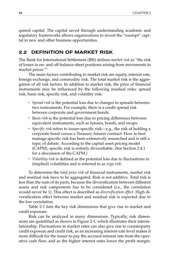
quired capital. The capital saved through understanding academic andregulatory frameworks allows organizations to invest the “exempt” capi-tal in new and other business opportunities.

2.2 DEFINITION OF MARKET RISK

The Bank for International Settlement (BIS) defines market risk as “the riskof losses in on- and off-balance-sheet positions arising from movements inmarket prices.”1

The main factors contributing to market risk are equity, interest rate,foreign exchange, and commodity risk. The total market risk is the aggre-gation of all risk factors. In addition to market risk, the price of financialinstruments may be influenced by the following residual risks: spreadrisk, basis risk, specific risk, and volatility risk:

• Spread risk is the potential loss due to changes in spreads betweentwo instruments. For example, there is a credit spread riskbetween corporate and government bonds.

• Basis risk is the potential loss due to pricing differences betweenequivalent instruments, such as futures, bonds, and swaps.

• Specific risk refers to issuer-specific risk—e.g., the risk of holding acorporate bond versus a Treasury futures contract. How to bestmanage specific risk has been extensively researched and is still atopic of debate. According to the capital asset pricing model(CAPM), specific risk is entirely diversifiable. (See Section 2.4.1for a discussion of the CAPM.)

• Volatility risk is defined as the potential loss due to fluctuations in(implied) volatilities and is referred to as vega risk.

To determine the total price risk of financial instruments, market riskand residual risk have to be aggregated. Risk is not additive. Total risk isless than the sum of its parts, because the diversification between differentassets and risk components has to be considered (i.e., the correlationwould never be 1). This effect is described as diversification effect. High di-versification effect between market and residual risk is expected due tothe low correlation.

Table 2-1 lists the key risk dimensions that give rise to market andcredit exposure.

Risk can be analyzed in many dimensions. Typically, risk dimen-sions are quantified as shown in Figure 2-1, which illustrates their interre-lationship. Fluctuations in market rates can also give rise to counterpartycredit exposure and credit risk, as an increasing interest-rate level makes itmore difficult for the issuer to pay the accrued interest rate from the oper-ative cash flow, and as the higher interest rates lower the profit margin.

34 CHAPTER 2


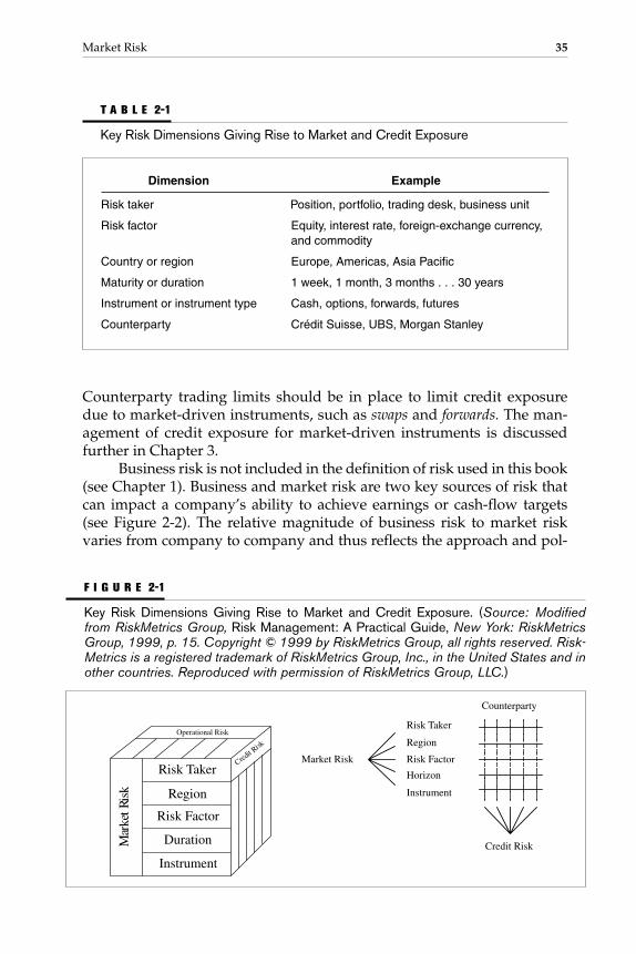
Counterparty trading limits should be in place to limit credit exposuredue to market-driven instruments, such as swaps and forwards. The man-agement of credit exposure for market-driven instruments is discussedfurther in Chapter 3.

Business risk is not included in the definition of risk used in this book(see Chapter 1). Business and market risk are two key sources of risk thatcan impact a company’s ability to achieve earnings or cash-flow targets(see Figure 2-2). The relative magnitude of business risk to market riskvaries from company to company and thus reflects the approach and pol-

Market Risk 35

T A B L E 2-1

Key Risk Dimensions Giving Rise to Market and Credit Exposure

Dimension Example

Risk taker Position, portfolio, trading desk, business unit

Risk factor Equity, interest rate, foreign-exchange currency, and commodity

Country or region Europe, Americas, Asia Pacific

Maturity or duration 1 week, 1 month, 3 months . . . 30 years

Instrument or instrument type Cash, options, forwards, futures

Counterparty Crédit Suisse, UBS, Morgan Stanley

Risk Taker

Region

Risk Factor

Horizon

Instrument

Market Risk

Counterparty

Credit RiskMar

ket R

isk

Risk Taker

Region

Risk Factor

Duration

Instrument

Credit R

isk

Operational Risk

F I G U R E 2-1

Key Risk Dimensions Giving Rise to Market and Credit Exposure. (Source: Modifiedfrom RiskMetrics Group, Risk Management: A Practical Guide, New York: RiskMetricsGroup, 1999, p. 15. Copyright © 1999 by RiskMetrics Group, all rights reserved. Risk-Metrics is a registered trademark of RiskMetrics Group, Inc., in the United States and inother countries. Reproduced with permission of RiskMetrics Group, LLC.)


icy for managing both types of risks; it also helps set the tone for a com-pany’s risk management culture and awareness. When discussing businessrisk, we are referring to the uncertainty (positive and negative) related tothe business decisions that companies make and to the business environ-ment in which companies operate. For example, business risk can arisefrom investment decisions and strategy, product development choices,marketing approaches, product placement issues, and client behavior un-certainty. Broadly speaking, these are decisions with an inherent long-termhorizon and involve structural risks that companies are “paid to take” inorder to generate profits. Companies evaluate and take business risks inareas based on their expertise and, to varying degrees, with significant in-fluence over potential returns. In contrast, market risk refers to the uncer-tainty of future financial results that arises from market-rate changes.

Market risk can impact on a company’s business in many differentways. For example, operating margins can be eroded due to the risingprices of raw materials or depreciating currencies in countries in which acompany has foreign sales (direct market risk impact). Changes in the mar-ket environment may eventually force companies to adjust the prices oftheir products or services, potentially altering sales volumes or competi-tiveness, depending on the positioning and market exposures of the com-pany’s competitors (the indirect impact of market risk on business results).Some organizations may be “paid” to take market risks (e.g., financial or-ganizations), but most seek to manage the impact of market risk on finan-cial results (this is especially true of most nonfinancial organizations).

Financial organizations have overlapping business and market risks.However, as their “raw materials” are currencies, interest rates, etc., fi-

36 CHAPTER 2

Operational

Systems

PeopleData quality

Controls

Transactions

MarketForeignexchange

Interest rate

Liquidity

Commodity

Equity

Business

Marketing

Sales

Reputation

Quality

Product placement

CreditDefault

Transition

Concentration Counterparty

CountryRecovery

F I G U R E 2-2

Differentiation Between Market Risk and Business Risk. (Source: Modified from Risk-Metrics Group, CorporateMetrics—Technical Document, New York: RiskMetrics Group,1999, p. 5, chart 1. Copyright © 1999 by RiskMetrics Group, all rights reserved.CorporateMetrics is a registered trademark of RiskMetrics Group, Inc., in the UnitedStates and in other countries. Reproduced with permission of RiskMetrics Group, LLC.)


nancial organizations have to keep business and market risks separated torealize success from intended business strategies and decisions, and fromthe risk-return relationship of these decisions.

2.3 CONCEPTUAL APPROACHES FOR MODELING MARKET RISK

Investment diversification was a well-established practice long beforeMarkowitz published his paper on portfolio selection in 1952.2 The devel-opment of the modern portfolio theory and of option pricing theories hadits roots some decades before Markowitz. These mostly quantitative ap-proaches were not the first to provide diversification for their customers,because such approaches were modeled on the investment trusts of Scot-land and England, which began in the middle of the nineteenth century,and diversification had occurred even earlier. In The Merchant of Venice,Shakespeare has the merchant Antonio say:

My ventures are not in one bottom trusted,Nor to one place; Nor is my whole estateUpon the fortune of this present year;Therefore, my merchandise makes me not sad.3

Prior to Markowitz’s 1952 article, there was no adequate quantita-tive theory of investment established that covered the effects of diversifi-cation when risks are correlated, distinguished between efficient andinefficient portfolios, and analyzed risk–return trade-offs on the portfolioas a whole. In order to understand the benefits and pitfalls of the theoriesand models currently used for regulatory and management purposes, it isnecessary to understand the development of portfolio theory. In 1935,Hicks discussed the need for an improved theory of money and the desir-ability of building a theory of money along the same lines as the alreadyexisting theory of value.4 Hicks introduced risk into his analysis. Specifi-cally, he noted: “The risk-factor comes into our problem in two ways: First,as affecting the expected period of investment, and second, as affectingthe expected net yield of investment.”5 Hicks represents the probabilitiesof risk dispersions by a mean value and by some appropriate measure ofdispersion. Hicks was a forerunner of Tobin6 in seeking to explain the de-mand for money as a consequence of the investor’s desire for low risk aswell as high return. Beyond that, there is little similarity between the twoauthors. Hicks, unlike Tobin or the appendix in Hicks7 (1962), did not des-ignate standard deviation or any other specific measure of dispersion asrepresenting risk for the purposes of analysis. Hicks could not demon-strate a formula relating risk on the portfolio to risk on individual assets.Hicks did not distinguish between efficient and inefficient portfolios,lacked a coherent image of an efficient frontier, and gave no hint of any

Market Risk 37


kind of theorem explaining that all efficient portfolios that include cashhave the same allocation of distribution among risky assets.

Hicks’s article on liquidity (1962) is more precise about the formula-tion of risk by mentioning the standard deviation as a measure of “cer-tainty” and the mean.8 The formalization was spelled out in a mathematicalappendix to Hicks (1962) titled “The Pure Theory of Portfolio Investment”and in a footnote on page 796 of the work that presents a µσ-efficient set di-agram. The appendix presents a mathematical model that is almost identi-cal to Tobin’s, but with no reference to Tobin’s work. The difference betweenthe Hicks and Tobin models is that Hicks assumed that all correlations arezero, whereas Tobin permitted any nonsingular covariance matrix. Specifi-cally, Hicks presented the general formula for portfolio variance, written interms of correlations rather than covariances. Hicks (1962) derived theTobin conclusion that among portfolios which include cash, there is a linearrelationship between portfolio mean and standard deviation, and that theproportions among risky assets remain constant along this linear portion ofthe efficient frontier. Hicks presented what later was called the Tobin separa-tion theorem.

Marschak (1938) was clearer in formulating risk by constructing anordinal theory of choice under uncertainty.9 He assumed a preference ordering in the space of parameters of probability distributions—in thesimplest form—expressed by the mean and the variance. From this for-mulation to the analysis of portfolio selection in general is the shortest ofsteps, but one not fully taken by Marschak,10 though he made tentativemoves in this direction, expressing preferences for investments by indif-ference curves in the mean-variance space. Marschak’s 1938 work is alandmark on the road to a theory of markets whose participants act underrisk and uncertainty, as later developed in Tobin11 and the CAPMs.12 It isthe most significant advance of economic theory regarding risk and un-certainty prior to the publication of von Neumann and Morgenstern in1944.13 The asset allocation decision had not been adequately addressedby neoclassical economists at the time of Marschak. The methodology ofdeterministic calculus is adequate for the decision of maximizing a con-sumer’s utility subject to a budget constraint (as part of the neoclassic ap-proach), whereas portfolio selection involves making a decision amidstuncertainty. Under these circumstances, the probabilistic notions of ex-pected return and risk become very important.

In 1938, Williams highlighted the importance of diversification.14 Heconcluded that probabilities should be assigned to possible values of a se-curity and the mean of these values used as the value of that security. Healso concluded that by investing in many securities, risk could be virtuallyeliminated. This presumption, that the law of large numbers applies to aportfolio of securities, cannot be accepted. The returns from securities aretoo intercorrelated. Diversification cannot eliminate all variance. Williams

38 CHAPTER 2


suggested that the way to find the value of a risky security has alwaysbeen to add a “premium for risk” to the pure interest rate, and then use thesum as the interest rate for discounting future receipts. Williams discussedthe separation of specific and systematic risk, without giving a clear over-all framework. It should be noted, however, that Williams’s “dividend dis-count model” remains one of the standard ways to estimate the securitymeans needed for a mean-variance analysis.15

Leavens’ 1945 article on the diversification of investments concludedthat each security is acted upon by independent causes.16 Leavens madethe assumptions behind the systemic/specific risk separation very clear,without directly tying his findings to a theoretical formulation.

2.4 MODERN PORTFOLIO THEORY

On the basis of his path-breaking 1952 article, Markowitz became thefather of modern portfolio theory (MPT).17 At the same time, Roy (1952)published an article on the same topic with similar conclusions and a cleartheoretical framework.18 The 1952 article on portfolio selection byMarkowitz proposed expected (mean) return, and variance of return, ofthe portfolio as a whole as criteria for portfolio selection, both as a possi-ble hypothesis about actual behavior and as a maxim for how investorsought to act. The article assumed that beliefs or projections about securitiesfollow the same probability rules that random variables obey. From thisassumption, Markowitz concluded that the expected return on the portfo-lio is a weighted average of the expected returns on individual securitiesand that the variance of return on the portfolio is a particular function ofthe variances of, and the covariances between, securities and their weightsin the portfolio. Markowitz distinguished between efficient and inefficientportfolios. Subsequently, this frontier became the “efficient frontier” forwhat Markowitz referred to as the set of mean-variance efficient combina-tions. Markowitz proposed that means, variances, and covariances of se-curities be estimated by a combination of statistical analyses. From theseestimates, the set of mean-variance efficient combinations can be derivedand presented to the investor, who can choose the desired risk-returncombination. Markowitz used geometrical analyses of various security ex-amples to illustrate properties of efficient sets, assuming nonnegative in-vestments subject to a budget constraint. He showed in his 1952 articlethat the set of efficient portfolios is piecewise linear (made up of con-nected straight lines) and the set of efficient mean-variance combinationsis piecewise parabolic.

Roy (1952) similarly proposed making choices on the basis of meanand variance of the portfolio as a whole. Specifically, he proposed choos-ing the positions that maximize the portfolio’s utility, based on the re-turn, with σ as the standard deviation of return. Roy’s formula for the

Market Risk 39


variance of the portfolio included the covariances of returns among secu-rities. The main differences between the Roy and Markowitz approacheswere that Markowitz required nonnegative investments, whereas Roy al-lowed the amount invested in any security to be positive or negative.Furthermore, Markowitz proposed allowing the investor to choose a de-sired portfolio from the efficient frontier, whereas Roy recommendedchoosing a specific portfolio. Roy’s 1952 article was his first and last arti-cle in finance. He made this one tremendous contribution and then dis-appeared from the field, whereas Markowitz wrote several books andmany articles on the portfolio-selection problem and enhancements ofhis 1952 article.19

The conceptual approach to market risk is closely linked historicallyto the development of modern portfolio theory and the option pricingtheory. Modern portfolio theory started with the path-breaking theory ofMarkowitz.20 Markowitz was the first finance theorist who explicitly in-cluded risk in portfolio analysis. The Markowitz approach is based on theassumption of a relation between risk and return and considers the effectof diversification, using the standard deviation or variance as a measurefor risk.

σ 2p = �

N

i = 1

X i2σ 2

1 + �N

i = 1�

N

j = 1

XiXjρijσiσj (2.1)

i ≠ 1

The portfolio return is the weighted return of the individual posi-tions, and the portfolio risk is the weighted risk of all individual assetsand the covariance between those assets:

–Rp = �

n

i = 1

Xiri

σ = �N

i = 1

X i2σ 2

1 + �N

i = 1�

N

j = 1

XiXjσij (2.2)

i ≠ 1

The covariance can be expressed as a correlation term as follows:

σij = ρijσiσj (2.3)

The risk-adjusted portfolio return is:

�rp

σ−p

rf� (2.4)

The efficient frontier is an outcome of Markowitz’s theory, a border-line of all portfolios with optimal risk–return relations (Figure 2-3). His ap-

40 CHAPTER 2


proach was developed further by Tobin.21 Tobin improved the correlationbetween the assets and the risk aversion by including a risk-free position.Through combining the portfolios on the efficient frontier of Markowitzand a risk-free position, Sharpe further developed the conceptual model-ing of market risks and introduced the capital market line as the tangentfrom the risk-free asset to the efficient frontier.

2.4.1 The Capital Asset Pricing Model

The complexity of Markowitz’s portfolio model and some generalizationof assumptions led to further developments. The capital asset pricingmodel (CAPM) was developed by Sharpe,22 Lintner,23 and Mossin,24 andlater was enhanced by Black. It is a logical extension of the ideas behindmodern portfolio theory as first outlined by Markowitz. Because theMarkowitz approach makes no statement about the pricing of equities, theCAPM offers a statement on the relevant investment risks and the risk–return relation under the condition that the markets are in equilibrium.The CAPM is an equilibrium model for the capital market.

Market Risk 41

rf

Risk σp

DCapital m

arket line

B

AC

Efficient frontier

Ret

urn

F I G U R E 2-3

Efficient Frontier Curve and Capital Market Line.


The CAPM is based on the following nine assumptions:25

• Utility maximization. Investors try to maximize their ownutilities; they are risk-averse.

• Decision basis. Investors make their decisions only on the basisof risk and return.

• Expectations. Investors have homogeneous expectationsregarding return and risk (variance and covariance) of the assets.

• One-period time horizon. Investors have identical time horizons ofone period.

• Information efficiency. Information is free and simultaneouslyavailable to all market participants.

• Risk-free asset. Investors can borrow or invest in an unlimitedamount of risk-free assets.

• Markets without friction. No taxes, transaction fees, restrictionson short positions or other market restrictions exist.

• Capital market equilibrium. The sum of all instruments is givenand in possession of the investors. All instruments aremarketable, and the assets are divisible to any degree. Supplyand demand are not influenced by anything other than price.

• Distribution. The CAPM, like the Markowitz approach, is basedon the normal distribution of returns or a quadratic utilityfunction.

All combinations are on the line between a risk-free investment andthe uncertain investment of the efficient frontier. The part between rf andD is called the capital market line (CML) and contains only one efficientportfolio, which is at the tangential point between the efficient frontierand the capital market line (see Figure 2-3).

It is not enough to know the return distribution (variance) of a posi-tion; the return must be viewed relative to the market and risk compo-nents. The CAPM assumes that a certain portion of the risk of a position isa reflection of the overall market risk, which is carried by all positions inthe market and thus cannot be diversified. This part of the risk is definedas systematic risk, which cannot be eliminated through diversification. Thisrisk premium is defined as the market risk premium. In contrast, the spe-cific risk (or unsystematic risk) cannot be explained by market events andhas its origins in position-specific factors (e.g., management errors andcompetitive disadvantages). This component can be diversified and is notrewarded by a premium.

The expected return of a specific stock is calculated as follows:

E (ri) = rf + βi ⋅ [E(rm) − rf] + εi (2.5)

42 CHAPTER 2


where ri = return of security irf = return of the risk-free asset

rm = return of the marketβi = sensitivity of security i relative to market movement mεi = error term

2.4.2 The Security Market Line

One of the key elements of modern portfolio theory is that, despite diver-sification, some risk still exists. The sensitivity of a specific position rela-tive to the market is expressed by βi (see Figure 2-4). The CAPM defines βi

as the relation of the systematic risk of a security i to the overall risk of themarket.

Market Risk 43

Exp

ecte

d re

turn

β

Security market line

m

rf

10

Investment in marketRisk free investment

rm

Expectedrisk

premium

Defensive Aggressive

F I G U R E 2-4

Security Market Line.


βi =�cov

vaarriiaann

ccee

((rr

m

m

,)

ri)� =

�βi = co

σvrm

(ri, rm)� (2.6)

where ri = return of security irf = return of the risk-free asset

rm = return of the marketβi = sensitivity of security i relative to market movement mεi = error term

The one-factor model is a strong simplification of the Markowitzmodel, and the CAPM is a theory. The main criticisms of the CAPM are asfollows:

• The market efficiency is not given in its strong form, as not all information is reflected in the market. This presents an opportunity for arbitrage profits, which can be generated as long as insider information is not available to the public.

• The normal distribution is a generalization, which distorts theresults, especially for idiosyncratic risks.

The main message of market efficiency as it pertains to capital mar-ket models is that a market is considered efficient if all available data andinformation are reflected in the pricing and in the demand-and-supply re-lation.26 Fama distinguishes three types of market efficiency: weak, semi-strong, and strong.27

In a study on Swiss equities, Zimmermann and Vock28 came to theconclusion that the test statistics (the standardized third and fourthmoment as a measure for the skewness and kurtosis, the standardizedspan or studentized range, and the test from Kolmogorov-Smirnov)point to a leptokurtic return distribution (see Figure 2-5). The studyconcluded that the normal distribution has to be questioned from astatistical point of view. The deviations are empirically marginal. Theleptokurtosis has been confirmed for U.S. equities in studies byFama,29 Kon,30 Westerfield,31 and Wasserfallen and Zimmermann32 (seeFigure 2-5). Zimmermann33 concluded that over a longer time horizon(1927 to 1987), the normal distribution fits the return distribution ofSwiss equities.

systematic risk of title i��risk of market portfolios

44 CHAPTER 2


2.4.3 Modified Form of CAPM by Black, Jensen, and Scholes

Black, Jensen, and Scholes conducted an empirical examination of theCAPM in 1972. They used a model without a risk-free interest rate, becausethe existence of a risk-free interest rate was controversial.34 In the modelwithout a risk-free return, the security market line (SML) is no longer de-fined by the risk-free return and the market portfolio; instead, it is a multi-tude of combinations, as there is a multitude of zero-beta portfolios.35

The return that they were able to explain was significantly higherthan the average risk-free return within the observation period. They con-cluded that the model is compatible with the standard form of the CAPM,but differentiates between borrowing and lending. The study supports thepractical observation that borrowing is more expensive than lendingmoney. Empirical studies support the development of the capital marketline with two interest rates, one for borrowing and one for lending money.It is an important improvement, as it excludes the assumption that bor-rowing and lending are based on the same risk-free rate.36 Figure 2-6 isbased on the following equations:

E(ri) = rL + βi ⋅ [E(rm) − rL] + εi (2.7)

E(ri) = rB + βi ⋅ [E(rm) − rB] + εi (2.8)

Market Risk 45

Prob

abili

ty %

Return

Normaldistribution

Leptokurtotic distribution

F I G U R E 2-5

Normal and Leptokurtic Distribution of Equity Returns.


2.4.4 Arbitrage Pricing Theory

Empirical examinations of the CAPM showed significant deficiencies inits ability to forecast and alleviate risk. These studies led to the develop-ment of the arbitrage pricing theory (APT), first introduced by Ross37 andfurther developed by other scientists.

APT is based on the empirical observation that different instrumentshave simultaneous and homogeneous development ranges. The theoryimplicitly assumes that the returns are linked to a certain number of fac-tors which influence the instrument prices. The part explained by thesefactors is assigned to the systematic factors, whereas the nonexplainablepart of the return (and thus the risk) is assigned to specific factors.

In theory, the factors are uncorrelated, as empirical examination sup-ports correlated factors. Such correlated factors have to be transformedinto an observation-equivalent model with uncorrelated factors. The fac-tors cannot be observed and have to be examined empirically.

A critical difference between CAPM and APT is that APT is an equi-librium theory, based on the arbitrage condition. As long as it is possiblewith intensive research to find factors that systematically impact the returnof a position, it is possible to do arbitrage based on this superior knowledge.

46 CHAPTER 2

rL

rB

D

B

AC

E

Efficient frontier

Risk σp

F I G U R E 2-6

Efficient Frontier with Different Interest Rates for Borrowing and Lending Capital.


2.4.5 Approaches to Option Pricing

Modern portfolio theory is not based solely on return calculations. Risk andrisk management become increasingly important. As the portfolio theoryshows, despite diversification, an investor is still exposed to systematic risk.With the development of portfolio and position insurance, an approach hasbeen created to hedge (insure) against unwanted moves of the underlyingposition. The theoretical framework introduced a range of applications,such as replication of indices, dynamic insurance, leveraging, immuniza-tion, structured products, etc. To understand the current state of option pric-ing, the different approaches, and the critics, it is necessary to summarizethe development of, and approaches to, modern option-valuation theory.

Valuation and pricing of income streams is one of the central prob-lems of finance. The issue seems straightforward conceptually, as itamounts to identifying the amount and the timing of the cash flows ex-pected from holding the claims and then discounting them back to thepresent. Valuation of a European-style call option requires that the mean ofthe call option’s payout distribution on the expiration date be estimated,and the discount rate be applied to the option’s expected terminal payout.

The first documented attempt to value a call option occurred nearthe turn of the twentieth century. Bachelier wrote in his 1900 thesis that thecall option can be valued under the assumption that the underlying claimfollows an arithmetic Brownian motion.38 Sprenkle and Samuelson used ageometric Brownian motion in their attempt to value options.39 As the un-derlying asset prices have multiplicative, rather than additive (as with thearithmetic motion) fluctuations, the asset price distribution at the expira-tion date is lognormal, rather then normal. Sprenkle and Samuelson’s re-search set the stage, but there was still a problem. Specifically, forimplementation of their approach, the risk-adjusted rates of price appreci-ation for both the asset and the option are required. Precise estimation wasthe problem, which was made more difficult as the option’s return de-pends on the asset’s return, and the passage of time.

The breakthrough came in 1973 with Black, Scholes, and Merton.40

They showed that as long as a risk-free hedge may be formed between theoption and its underlying asset, the value of an option relative to the assetwill be the same for all investors, regardless of their risk preferences. Theargument of the risk-free hedge is convincing, because in equilibrium, noarbitrage opportunities can exist, and any arbitrage opportunity is obvi-ous for all market participants and will be eliminated. If the observedprice of the call is above (or below) its theoretical price, risk-free arbitrageprofits are possible by selling the call and buying (or selling) a portfolioconsisting of a long position in a half unit of the asset, and a short positionin the other half in risk-free bonds. In equilibrium, no arbitrage opportu-nities can exist, and any arbitrage opportunity can exist.

Market Risk 47


2.4.5.1 Analytical FormulasThe option valuation theory goes beyond the mathematical part of the for-mula. The economic insight is that if a risk-free hedge between the optionand its underlying asset my be formed, risk-neutral valuation may be ap-plied. The Black-Scholes model follows the work of Sprenkle and Samuel-son. In a risk-neutral market, all assets (and options) have an expected rateof return equal to the risk-free interest rate. Not all assets have the sameexpected rate of price appreciation. Some assets, such as bonds, havecoupons, and equities have dividends. If the asset’s income is modeled asa constant and continuous proportion of the asset price, the expected rateof price appreciation on the asset equals the interest rate less the cash dis-bursement rate. The Black-Scholes formula covers a wide range of under-lying assets. The distinction between the valuation problems described asfollows rests in the asset’s risk-neutral price appreciation parameter:

• Non-dividend-paying stock options. The best-known optionvaluation problem is that of valuing options on non-dividend-paying stocks. This is, in fact, the valuation problem addressed byBlack and Scholes in 1973.41 With no dividends paid on theunderlying stock, the expected price appreciation rate of the stockequals the risk-free rate of interest, and the call option valuationequation becomes the familiar Black-Scholes formula.

• Constant-dividend-yield stock options. Merton generalized stockoption valuation in 1973 by assuming that stocks pay dividendsat a constant, continuous dividend yield.42

• Futures options. Black valued options on futures in 1976.43 In arisk-neutral world with constant interest rates, the expected rateof price appreciation on a futures contract is zero, because itinvolves no cash outlay.

• Futures-style futures options. Following the work of Black, Asayvalued futures-style futures options.44 Such options, traded onvarious exchanges, have the distinguishing feature that theoption premium is not paid up front. Instead, the option positionis marked to market in the same manner as the underlyingfutures contract.

• Foreign currency options. Garman and Kohlhagen valued optionson foreign currency in 1983.45 The expected rate of priceappreciation of a foreign currency equals the domestic rate ofinterest less the foreign interest.

• Dynamic portfolio insurance. Dynamic replication is at the heartof one of the most popular financial products of the 1980s—dynamic portfolio insurance. Because long-term index putoptions were not traded at the time, stock portfolio managers had

48 CHAPTER 2


to create their own insurance by dynamically rebalancing aportfolio consisting of stocks and risk-free bonds. The weights inthe portfolio show that as stock prices rise, funds are transferredfrom bonds to stocks, and vice versa.

• Compound options. An important extension of the Black-Scholesmodel that falls in the single underlying asset category is thecompound option valuation theory developed by Geske.46

Compound options are options on options. A call on a call, forexample, provides its holder with the right to buy a call on theunderlying asset at some future date. Geske shows that if theseoptions are European-style, valuation formulas can be derived.

• American-style call options on dividend-paying stocks. The Geskecompound option model has been applied in other contexts. Roll,Geske, and Whaley developed a formula for valuing anAmerican-style call option on a stock with known discretedividends.47 If a stock pays a cash dividend during the call’s life,it may be optimal to exercise the call early, just prior to dividendpayment. An American-style call on a dividend-paying stock,therefore, can be modeled as a compound option providing itsholder with the right, on the ex-dividend date, either to exerciseearly and collect the dividend, or to leave the position open.

• Chooser options. Rubinstein used the compound optionframework in 1991 to value the “chooser” or “as-you-like-it”options traded in the over-the-counter market.48 The holder of achooser option has the right to decide at some future datewhether the option is a call or a put. The call and the put usuallyhave the same exercise price and the same time remaining toexpiration.

• Bear market warrants with a periodic reset. Gray and Whaley usedthe compound option framework to value yet another type ofcontingent claim, S&P 500 bear market warrants with a periodicreset traded on the Chicago Board Options Exchange and theNew York Stock Exchange.49 The warrants are originally issued asat-the-money put options but have the distinguishing feature thatif the underlying index level is above the original exercise onsome prespecified future date, the exercise price of the warrant isreset at the then-prevailing index level. These warrants offer anintriguing form of portfolio insurance whose floor value adjustsautomatically as the index level rises. The structure of thevaluation problem is again a compound option, and Gray andWhaley’s 1997 paper provides the valuation formula.

• Lookback options. A lookback option is another exotic that hasonly one underlying source of price uncertainty. Such an option’s

Market Risk 49


exercise price is determined at the end of its life. For a call, theexercise price is set equal to the lowest price that the assetreached during the life of the option; for a put, the exercise priceequals the highest asset price. These buy-at-the-low and sell-at-the-high options can be valued analytically. Formulas areprovided in Goldman, Sosin, and Gatto’s 1979 paper.50

• Barrier options. Barrier options are options that either cease toexist or come into existence when some predefined asset pricebarrier is hit during the option’s life. A down-and-out call, forexample, is a call that gets knocked out when the asset price fallsto some prespecified level prior to the option’s expiration.Rubinstein and Reiner’s 1991 paper provides valuation equationsfor a large family of barrier options.51

2.4.5.2 Approximation MethodsMany valuation problems do not have explicit closed-form solutions.Probably the best-known example of this is the valuation of American-style options. With American-style options, the option holder has an infi-nite number of exercise opportunities between the current date and theoption’s expiration date, making the problem challenging from a mathe-matical standpoint. Hundreds of different types of exotic options trade inthe OTC market, and many, if not most, do not have analytical formulas.Nonetheless, they can all be valued accurately using the Black-Scholesmodel. If a risk-free hedge can be formed between the option and the un-derlying asset, the Black-Scholes model risk-neutral valuation theory canbe applied, albeit using numerical methods. A number of numerical methods for valuing options are lattice based. These methods replace theBlack-Scholes model assumption that asset price moves smoothly andcontinuously through time with an assumption that the asset price movesin discrete jumps over discrete intervals during the option’s life:

• Binomial method. Perhaps the best-known lattice-based method isthe binomial method, developed independently in 1979 by Cox,Ross, and Rubinstein and Rendleman and Bartter.52 In thebinomial method, the asset price jumps up or down, by a fixedproportion, at each of a number of discrete time steps during theoption’s life. The length of each time step is determined when theuser specifies the number of time steps. The greater the number oftime steps, the more precise the method. The cost of the increasedprecision, however, is computational speed. With n time steps, 2nasset price paths over the life of the option are considered. With 20time steps, this means more than 1 million paths.

The binomial method has wide applicability. Aside from theAmerican-style option feature, which is easily incorporated

50 CHAPTER 2


within the framework, the binomial method can be used to valuemany types of exotic options. Knockout options, for example, canbe valued using this technique. One simply imposes a differentcheck on the calculated option values at the nodes of the interme-diate time steps between 0 and n, i.e., if the underlying asset pricefalls below the option’s barrier, the option value at that node isset equal to 0. The method can also be extended to handle multi-ple sources of asset price uncertainty. Boyle, Evnine, and Gibbsadapt the binomial procedure to handle exotics with multiplesources of uncertainty, including options on the minimum andmaximum, spread options, and so on.53

• Trinomial method. The trinomial method is another popularlattice-based method. As outlined by Boyle, this method allowsthe asset to move up, move down, or stay the same at each timeincrement.54 Again, the parameters of the discrete distribution arechosen in a manner consistent with the lognormal distribution,and the procedure begins at the end of the option’s life and worksbackward. By having three branches instead of two, the trinomialmethod provides greater accuracy than the binomial method for agiven number of time steps. The cost, of course, is that the greaterthe number of branches, the slower the computational speed.

• Finite difference method. The explicit finite difference method wasthe first lattice-based procedure to be applied to option valuation.Schwartz applied it to warrants, and Brennan and Schwartzapplied it to American-style put options on common stocks.55 Thefinite difference method is similar to the trinomial method in thesense that the asset price moves up, moves down, or stays thesame at each time step during the option’s life. The difference inthe techniques arise only from how the price increments and theprobabilities are set. In addition, finite difference methods calculatean entire rectangle of node values rather than simply a tree.

• Monte Carlo simulation. Boyle introduced Monte Carlo simulationto option valuation.56 Like the lattice-based procedures, thetechnique involves simulating possible paths that the asset pricemay take over the life of the option. Again, the simulation isperformed in a manner consistent with the lognormal asset priceprocess. To value a European-style option, each sample run isused to produce a terminal asset price, which, in turn, is used todetermine the terminal option value. With repeated sample runs, adistribution of terminal options values is obtained, and theexpected terminal option value may be calculated. This expectedvalue is then discounted to the present to obtain the optionvaluation. An advantage of the Monte Carlo method is that the

Market Risk 51


degree of valuation error can be assessed directly, using thestandard error of the estimate. The standard error equals thestandard deviation of the terminal option values divided by thesquare root of the number of trials. Another advantage of theMonte Carlo technique is its flexibility. Because the path of theasset price beginning at time 0 and continuing throughout the lifeof the option is observed, the technique is well suited for handlingbarrier-style options, Asian-style options, Bermuda-style options,and the like. Moreover, it can easily be adapted to handle multiplesources of price uncertainty. The technique’s chief disadvantage isthat it can be applied only when the option payout does notdepend on its value at future points in time. This eliminates thepossibility of applying the technique to American-style optionvaluation, in which the decision to exercise early depends on thevalue of the option that will be forfeit.

• Compound option approximation. The quasi-analytical methodsfor option valuation are quite different from the procedures thatattempt to describe asset price paths. Geske and Johnson, forexample, use a Geske compound option model to develop anapproximate value for an American-style option.57 The approachis intuitively appealing. An American-style option, after all, is acompound option with an infinite number of early exerciseopportunities. While valuing an option in this way makesintuitive sense, the problem is intractable from a computationalstandpoint. The Geske-Johnson insight is that although wecannot value an option with an infinite number of early exerciseopportunities, we can extrapolate its value by valuing a sequenceof “pseudo-American” options with zero, one, two, and perhapsmore early exercise opportunities at discrete, equally spacedintervals during the option’s life. The advantage that this offers isthat each of these options can be valued analytically. With eachnew option added to the sequence, however, the valuation of ahigher-order multivariate normal integral is required. With noearly exercise opportunities, only a univariate function isrequired. However, with one early exercise opportunity, abivariate function is required; with two opportunities, a trivariatefunction is required, and so on. The more of these options used inthe series, the greater the precision in approximating the limitingvalue of the sequence. The cost of increased precision is thathigher-order multivariate integral valuations are time-consumingcomputationally.

• Quadratic approximation. Barone-Adesi and Whaley presented aquadratic approximation in 1987.58 Their approach, based on the

52 CHAPTER 2


work of MacMillan, separates the value of an American-styleoption into two components: the European-style option value andan early exercise premium.59 Because the Black-Scholes modelformula provides the value of the European-style option, theyfocus on approximating the value of the early exercise premium.By imposing a subtle change on the Black-Scholes model partialdifferential equation, they obtain an analytical expression for theearly exercise premium, which they then add to the European-style option value, thereby providing an approximation of theAmerican-style option value. The advantages of the quadraticapproximation method are speed and accuracy.

2.4.5.3 GeneralizationsThe generalizations of the Black-Scholes option valuation theory focus onthe assumed asset price dynamics. Some examine the valuation implica-tions of modeling the local volatility rate as a deterministic function of theasset price or time or both. Others examine the valuation implicationswhen volatility, like asset price, is stochastic.

Under the assumption that the local volatility rate is a deterministicfunction of time or the asset price or both, the Black-Scholes model risk-free hedge mechanisms are preserved, so risk-neutral valuation remainspossible. The simplest in this class of models is the case in which the localvolatility rate is a deterministic function of time. For this case, Mertonshowed that the valuation equation for a European-style call option is theBlack-Scholes model formula, where the volatility parameter is the aver-age local volatility rate over the life of the option.60

Other models focus on the relationship between asset price andvolatility and attempt to account for the empirical fact that, in at leastsome markets, volatility varies inversely with the level of asset price. Onesuch model is the constant elasticity of variance model proposed by Coxand Ross.61 However, valuation can be handled straightforwardly usinglattice-based or Monte Carlo simulation procedures.

Derman and Kani, Dupire, and Rubinstein and Reiner recently de-veloped a valuation framework in which the local volatility rate is a de-terministic (but unspecified) function of asset price and time.62 If thespecification of the volatility function is known, any of the lattice-based orsimulation procedures can be applied to option valuation. Unfortunately,the structural form is not known. To circumvent this problem, these au-thors parameterize their model by searching for a binomial or trinomiallattice that achieves an exact cross-sectional fit of reported option prices.An exact cross-sectional fit is always possible, because there are as manydegrees of freedom in defining the lattice (and, hence, the local volatility-rate function) as there are option prices. With the structure of the implied

Market Risk 53


tree identified, it becomes possible to value other, more exotic, OTC op-tions and to refine hedge ratio computations.

The effects of stochastic volatility on option valuation are modeledby either superimposing jumps on the asset price process or allowingvolatility to have its own diffusion process or both. Unfortunately, the in-troduction of stochastic volatility negates the Black-Scholes model risk-free hedge argument, because volatility movements cannot be hedged. Anexception to this rule is provided by Merton, who adds a jump term to theusual geometric Brownian motion governing asset price dynamics.63 Byassuming that the jump component of an asset’s return is unsystematic,the Merton model can create a risk-free portfolio in the Black-Scholesmodel sense and apply risk-neutral valuation. Indeed, Merton finds ana-lytical valuation formulas for European-style options. If the jump risk issystematic, however, the Black-Scholes model risk-free hedge cannot beformed, and option valuation will be utility-dependent.

A number of authors model asset price and asset price volatility asseparate, but correlated, diffusion processes. Asset price is usually as-sumed to follow geometric Brownian motion. The assumptions governingvolatility vary. Hull and White, for example, assume that volatility followsgeometric Brownian motion.64 Scott models volatility using a mean-reverting process, and Wiggins uses a general Wiener process.65 Batescombines both jump and volatility diffusions in valuing foreign currencyoptions. Except in the uninteresting case in which asset price and volatil-ity movements are independent, these models require the estimation ofrisk premiums.66 The problem when volatility is stochastic is that a risk-free hedge cannot be created, because volatility is not a traded asset. Butperhaps this problem is only temporary. The critical issue for all options,of course, is correct contract design.

2.5 REGULATORY INITIATIVES FOR MARKETRISKS AND VALUE AT RISK

Alan Greenspan has made it very clear that the assumptions and condi-tions must be fully discussed and understood when applying quantitativemodels such as value at risk (VaR):

Probability distributions estimated largely, or exclusively, over cycles thatdo not include periods of panic will underestimate the likelihood of extremeprice movements because they fail to capture a secondary peak at the ex-treme negative tail that reflects the probability of occurrence of a panic. Fur-thermore, joint distributions estimated over periods that do not includepanics will underestimate correlations between asset returns during panics.Under these circumstances, fear and disengagement on the part of investorsholdings net long positions often lead to simultaneously declines in the val-ues of private obligations, as investors no longer realistically differentiate

54 CHAPTER 2


among degrees of risk and liquidity, and to increase in the values of risklessgovernment securities. Consequently, the benefits of portfolio diversifica-tion will tend to be overestimated when the rare panic periods are not takeninto account.67

The 1988 Basel accord provided the first step toward tighter riskmanagement and enforceable international regulation with similar struc-tural conditions for financial supervision.68 The Basel accord set minimumcapital requirements that must be met by banks to guard against creditrisk. This agreement led to a still-evolving framework to impose capitaladequacy requirements to guard against market risks.

The reasoning behind regulation is multilayered and complex. Onecould ask why regulations are necessary. In a free market, investors shouldbe free to invest in firms that they believe to be profitable, and as owners ofan institution, they should be free to define the risk profile within whichthe institution should be free to act and evolve. Essentially, this is whathappened to Barings, where complacent shareholders failed to monitor thefirm’s management (see Section 6.6). Poor control over traders led to in-creasingly risky activities and, ultimately, bankruptcy. In freely functioningcapital markets, badly managed institutions should be allowed to fail. Suchfailures also serve as powerful object lessons in risk management.

Nevertheless, supervision is generally viewed as necessary whenfree markets appear to be unable, themselves, to allocate resources effi-ciently. For financial institutions, this is the rationale behind regulations toprotect against systemic risk (externalities) and to protect client assets (i.e.,deposit insurance).

Systemic risk arises when an institution’s failure affects other partic-ipants in the market. Here the fear is that a default by one institution willhave a cascading effect on other institutions, thus threatening to destabi-lize the entire financial system. Systemic risk is rather difficult to evaluate,because it involves situations of extreme instability, which happen infre-quently. In addition, regulators tend to take preventive measures to pro-tect the system before real systemic damage is caused.69

Deposit insurance also provides a rationale for regulative measures.By nature, bank deposits have destabilizing potential. Depositors arepromised that the full face value of their investments will be repaid on de-mand. If customers fear that a bank’s assets have fallen behind its liabili-ties, they may then rationally trigger a run on the bank. Given that banksinvest in illiquid assets, including securities and real estate, the demandfor repayment will force liquidation at great cost.

One solution to this problem is government guarantees on bank de-posits, which reduce the risk of bank runs. These guarantees are alsoviewed as necessary to protect small depositors who have limited finan-cial experience and cannot efficiently monitor their banks.

Market Risk 55


There is an ongoing argument that deposit insurance could be pro-vided by the private sector instead of the government. Realistically, how-ever, private financial organizations may not be able to provide financialtransfers to investors if large macroeconomic shocks or sector collapsesoccur, such as the U.S. savings and loan crisis of the 1980s. On the otherhand, applying Darwinism to capital markets, it should be possible toeliminate failing institutions from the market and replace them with fitterorganizations.70

This government guarantee is no “panacea, for it creates a host ofother problems, generally described under the rubric of moral hazard (seeSection 1.4). Given government guarantees, there is even less incentive fordepositors to monitor their banks. As long as the cost of the deposit insur-ance is not related to the risk-profile of the activities, there will be perverseincentives to take additional risks. The moral hazard problem, due to de-posit insurance, is a rationale behind regulatory attempts to superviserisk-taking activities. This is achieved by regulating the bank’s minimumlevels of capital, providing a reserve for failures of the institution or sys-temic risks. Capital adequacy requirements can also serve as a deterrent tounusual risk taking if the amount of capital set aside is tied to the amountof risk undertaken.

Alan Greenspan stated in 1999 that the current regulatory standardshad been misused due to inconsistent and arbitrary treatment:

The current international standards for bank capital had encouraged banktransactions that reduce regulatory requirements more than they reduce abank’s risk position. The fundamental credibility of regulatory capital stan-dards as a tool for prudential oversight and prompt corrective action at thelargest banking organizations has been seriously undermined.71

2.5.1 Development of an International Framework for Risk Regulation

The Basel Committee on Banking Supervision was founded in 1975; it is thedriving force for harmonization of banking supervision regulation on an in-ternational level, and it substantially supports cross-border enforcement ofcooperation among national regulators. The committee’s recommendationshave no internal binding power, but based on the material power of per-suasion and the implementation of its recommendations at the local level bythe members of the Committee, it has a worldwide impact.72

Capital adequacy is the primary focus of the committee, as capitalcalculation has a central role in all local regulations, and the standards ofthe BIS are broadly implemented. The standards are intended tostrengthen the international finance system and reduce the distortion ofnormal trading conditions by arbitrary national requirements. The BIS

56 CHAPTER 2


recommendations apply only to international banks and consolidatedbanking groups. They are minimum standards, allowing local regulatorsto set or introduce higher requirements. The Basel Committee intends todevelop and enhance an international regulatory network to increase thequality of banking supervision worldwide.

2.5.2 Framework of the 1988 BIS Capital Adequacy Calculation

Since its inception, the Basel Committee has been very active on the issueof capital adequacy. A landmark financial agreement was reached withthe Basel accord, concluded on July 15, 1988, by the central bankers ofthe G-10 countries.73 The regulators announced that the accord would re-sult in international convergence of supervisory regulations governingthe capital adequacy of international banks. Though minimal, these cap-ital adequacy standards increase the quality and stability of the interna-tional banking system, and thus help to reduce distortion betweeninternational banks. The main purpose of the 1988 Basel accord was toprovide general terms and conditions for commercial banks by means ofa minimum standard of capital requirements to be applied in all membercountries. The accord contained minimal capital standards for the supportof credit risks in balance and off-balance positions, as well as a definitionof the countable equity capital. The Basel capital accord was modified in1994 and 1995 with regard to derivatives instruments and recognition ofbilateral netting agreements.74

With the Cooke defined ratio, the 1988 accord created a commonmeasure of solvency. However, it covers only credit risks and thus dealssolely with the identity of banks’ debtors. The new ratios became bindingby regulation in 1993, covering all insured banks of the signatory countries.

2.5.2.1 The Cooke RatioThe Basel accord requires that banks hold capital equal to at least 8 percentof their total risk-weighted assets. Capital, however, is interpreted morebroadly than the usual definition of equity, because its goal is to protectdeposits. It consists of two components:

• Tier 1 capital. Tier 1 capital, or core capital, includes stock issuesand disclosed reserves. General loan loss reserves constitutecapital that has been dedicated to funds to absorb potential futurelosses. Real losses in the future are funded from the reserveaccount rather than through limitation of earnings, smoothingout income over time.

• Tier 2 capital. Tier 2 capital, or supplementary capital, includesperpetual securities, undisclosed reserves, subordinated debt

Market Risk 57


with maturity longer than five years, and shares redeemable atthe option of the issuer. Because long-term debt has a juniorstatus relative to deposits, debt acts as a buffer to protectdepositors (and the deposit insurer).

The Cooke ratio requires an 8 percent capital charge, at least 50 per-cent of which must be covered by Tier 1 capital. The general 8 percent cap-ital charge is multiplied by risk capital weights according to predeterminedasset classes. Government bonds, such as Treasuries, Bundesobligationen,Eidgenossen, and so forth are obligations allocated to the Organization forEconomic Cooperation and Development (OECD) government papers,which have a risk weight of zero. In the same class fall cash and gold heldby banks. As the perceived credit risk increases (nominally), so does therisk weight. Other asset classes, such as claims on corporations (includingloans, bonds, and equities), receive a 100 percent weight, resulting in therequired coverage of 8 percent of capital.

Signatories of the Basel accord are free to impose higher local capitalrequirements in their home countries.75 For example, under the newly es-tablished bank capital requirements, U.S. regulators have added a capitalrestriction which requires that Tier 1 capital must comprise no less than 3percent of total assets.

2.5.2.2 Activity RestrictionsIn addition to the weights for the capital adequacy calculation, the Baselaccord set limits on excessive risk taking. These restrictions relate to largerisks, defined as positions exceeding 10 percent of the bank’s capital.Large risks must be reported to regulatory authorities on a formal basis.Positions exceeding 25 percent of the bank’s capital are not allowed (un-less a bank has the approval of the local regulator). The sum of all large-risk exposures may not exceed 800 percent of the capital.

2.5.3 Criticisms of the 1988 Approach

The 1988 Basel accord had several drawbacks, which became obviouswith implementation. The main criticisms were the lack of accommoda-tion of the portfolio approach, the lack of netting possibilities, and the wayin which market risks were incorporated.

• The portfolio approach was not accommodated. Thus, correlationsbetween different positions of the bank’s portfolio did notaccount for the portfolio risk of the bank’s activities. The Baselaccord increased the capital requirements resulting from hedgingstrategies, as offsetting hedging positions were not allowed.

• Netting was not allowed. If a bank nets corresponding lendersand borrowers, the total net exposure may be small. If a

58 CHAPTER 2


counterparty fails to fulfill its obligations, the overall loss may bereduced, as the positions lent are matched by the positionsborrowed. Netting was an important driving force behind thecreation of swaps and time deposits. Swaps (of currencies andinterest rates) are derivatives contracts involving a series ofexchanges of payments and are contracted with explicit offsetprovisions. In the event of a counterparty default, the bank isexposed only to the net of the interest payments, not to thenotional amount.76

• Exposures to market risk were vaguely regulated. According to the1988 Basel accord, assets were recorded at book value. Thesepositions could deviate substantially from their current marketvalues. As a result, the accounting approach created a potentialsituation in which an apparently healthy balance sheet withacceptable capital (recorded at book value) hid losses in marketvalue. This regulatory approach concerning accounting createdproblems for the trading portfolios of banks with substantialpositions in derivatives. This specific drawback convinced theBasel Committee to move toward measuring market risk by thevalue-at-risk approach and mark-to-market position booking.

2.5.4 Evolution of the 1996 Amendment on Market Risks

In view of the increasing exposure to market risks in securities and de-rivatives trading, the Basel Committee created a substantial enhancementof the credit-risk-oriented capital adequacy regulations through newmeasurement rules and capital requirements to support market risksthroughout an institution. The committee published the results of itswork for discussion in January 1996.77 The discussion paper proposedtwo alternative methods for risk measurement and capital requirementsto support market risks. The standard model approach was to be used bysmall and midsized banks lacking the complex technological infrastruc-ture and expertise needed to calculate daily market risk exposures. Theinternal model approach could be used if the local regulator explicitly al-lowed the bank to use its own technological infrastructure and expertiseto calculate daily market risk exposures. Banks would have the opportu-nity to use both approaches simultaneously during a transition period.After a certain time, banks would be expected to use only one modelacross the institution.

Originally, the aim had been for a harmonized standard, whichshould have balanced the terms of competition between the securitiesdealers and the banks regarding capital requirements. The developmentof such a regulative framework would have been supported by a joint

Market Risk 59


project between the Basel Committee and the stock exchange supervisoryauthorities, for whom market risks have always been in the foreground.The discussion with the Technical Committee of the International Organi-zation of Securities Commission (IOSCO)—the international associationof supervisory authorities of the securities houses of the Western industri-alized nations—failed, because the IOSCO members could not agree on acommon approach. Partly responsible for the failure was the fact thatIOSCO had no concrete capital adequacy standard. This would have re-quired a substantial reworking of IOSCO’s regulations.

Based on this discussion, the Basel Committee published a first con-sultation paper in 1993, which included proposals for the regulatory treat-ment of market risks of debt and equity positions in the trading books. Fortrading positions, the related derivatives instruments, and foreign cur-rency risks from the banking books, the committee proposed a bindingstandard approach for measurement and capital requirements to supportmarket risks. In addition, a proposal for the measurement of interest raterisks based on the bank’s complete activity has been developed to identifyunexceptionally high interest rate risks (the so-called outlier concept). Asan alternative to the proposed standard approach for the measurementand capital requirements to support market risks, the committee also con-sidered the banks’ own internal models for the measurement and capitalrequirements to support market risks. The modified recommendations ofthe Basel Committee were published in April 1995. Simultaneously, an-other globally coordinated consultation procedure was carried out withmarket participants and representatives from the local regulators. Thefinal capital adequacy accord for measurement and capital requirementsto support market risks was adopted by the committee in December 1995and published in January 1996. The member countries had until the end of1997 to include the modified capital adequacy regulation in their nationalsupervisory regulations.

2.6 AMENDMENT TO THE CAPITAL ACCORD TO INCORPORATE MARKET RISKS

Starting at the end of 1997, or earlier, if their supervisory authority soprescribed, banks were required to measure and apply capital charges totheir market risks in addition to their credit risks.78 Market risk is definedas “the risk of losses in on- and off-balance-sheet positions arising frommovements in market prices.” The following risks are subject to this requirement:

• Risks pertaining to interest-rate-related instruments and equitiesin the trading book

• Foreign exchange risk and commodities risk throughout the bank

60 CHAPTER 2


2.6.1 Scope and Coverage of Capital Charges

The final version of the amendment to the capital accord to incorporatemarket risks regulates capital charges for interest-rate-related instrumentsand equities and applies to the current market value of items in the bank’strading books. By trading book is meant the bank’s proprietary positions infinancial instruments (including positions in derivative products and off-balance-sheet instruments) which are intentionally held for short-term re-sale. The financial instruments may also be acquired by the bank with theintention of benefiting in the short term from actual or expected differencesbetween their buying and selling prices, or from other price or interest-ratevariations; positions in financial instruments arising from matched princi-pal brokering and market making; or positions taken in order to hedgeother elements of the trading book.79

Capital charges for foreign exchange risk and for commodities riskapply to the bank’s total currency and commodity positions, subject tosome discretion to exclude structural foreign exchange positions:

For the time being, the Committee does not believe that it is necessary toallow any de minimis exemptions from the capital requirements for marketrisk, except for those for foreign exchange risk set out in paragraph 13 of A.3,because the Capital Accord applies only to internationally active banks, andthen essentially on a consolidated basis; all of these are likely to be involvedin trading to some extent.80

2.6.2 Countable Capital Components

The definition of capital is based on that of the BIS, from the Amendment tothe Capital Accord to Incorporate Market Risks:

The principal form of eligible capital to cover market risks consists ofshareholders’ equity and retained earnings (tier 1 capital) and supple-mentary capital (tier 2 capital) as defined in the 1988 Accord. But banksmay also, at the discretion of their national authority, employ a third tierof capital (“tier 3”), consisting of short-term subordinated debt as de-fined in paragraph 2 below for the sole purpose of meeting a proportionof the capital requirements for market risks, subject to the followingconditions. . . .81

The definition of eligible regulatory capital remains the same as out-lined in the 1988 accord and clarified in the October 27, 1998, press releaseon instruments eligible for inclusion in Tier 1 capital. The ratio must be nolower than 8 percent for total capital. Tier 2 capital continues to be limitedto 100 percent of Tier 1 capital.82

To clarify the impact of the amendment for market risk on the risksteering of the banks, the capital definitions are summarized as follows:

Market Risk 61


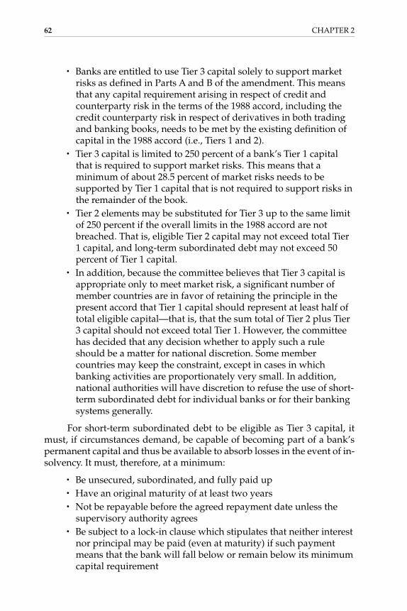
• Banks are entitled to use Tier 3 capital solely to support marketrisks as defined in Parts A and B of the amendment. This meansthat any capital requirement arising in respect of credit andcounterparty risk in the terms of the 1988 accord, including thecredit counterparty risk in respect of derivatives in both tradingand banking books, needs to be met by the existing definition ofcapital in the 1988 accord (i.e., Tiers 1 and 2).

• Tier 3 capital is limited to 250 percent of a bank’s Tier 1 capitalthat is required to support market risks. This means that aminimum of about 28.5 percent of market risks needs to besupported by Tier 1 capital that is not required to support risks inthe remainder of the book.

• Tier 2 elements may be substituted for Tier 3 up to the same limitof 250 percent if the overall limits in the 1988 accord are notbreached. That is, eligible Tier 2 capital may not exceed total Tier1 capital, and long-term subordinated debt may not exceed 50percent of Tier 1 capital.

• In addition, because the committee believes that Tier 3 capital isappropriate only to meet market risk, a significant number ofmember countries are in favor of retaining the principle in thepresent accord that Tier 1 capital should represent at least half oftotal eligible capital—that is, that the sum total of Tier 2 plus Tier3 capital should not exceed total Tier 1. However, the committeehas decided that any decision whether to apply such a ruleshould be a matter for national discretion. Some membercountries may keep the constraint, except in cases in whichbanking activities are proportionately very small. In addition,national authorities will have discretion to refuse the use of short-term subordinated debt for individual banks or for their bankingsystems generally.

For short-term subordinated debt to be eligible as Tier 3 capital, itmust, if circumstances demand, be capable of becoming part of a bank’spermanent capital and thus be available to absorb losses in the event of in-solvency. It must, therefore, at a minimum:

• Be unsecured, subordinated, and fully paid up• Have an original maturity of at least two years• Not be repayable before the agreed repayment date unless the

supervisory authority agrees• Be subject to a lock-in clause which stipulates that neither interest

nor principal may be paid (even at maturity) if such paymentmeans that the bank will fall below or remain below its minimumcapital requirement

62 CHAPTER 2


2.6.3 The de Minimis Rule

The Basel Committee has ruled out the use of simplifying approaches, al-lowing small institutions with negligible exposures to be excluded fromthe capital requirement for market risks:

For the time being, the Committee does not believe that it is necessary toallow any de minimis exemptions from the capital requirements for marketrisk, except for those for foreign exchange risk set out in paragraph 13 of A.3,because the Capital Accord applies only to internationally active banks, andthen essentially on a consolidated basis; all of these are likely to be involvedin trading to some extent.83

However, several countries, such as Germany and Switzerland, have in-cluded de minimis rules in their national regulations, especially with re-gard to asset management–oriented institutions which have negligiblemarket risk positions.84 Assuming the approval of the national authorities(subject to compliance with the criteria for de minimis exception), localsupervisors are free to monitor the relevant exposures in the non–de min-imis institutions more carefully. The approach is reasonable for smallerasset management and private banking institutions, which do not takesubstantial amounts of risk on their own books, as they execute on behalfof their clients. The important distinction is between organizations sub-ject to the standard model approach and those subject to the internalmodel approach, as this difference determines how risk has to be sup-ported by capital. Thus it fixes capital that could be used for other busi-ness purposes.85

2.7 THE STANDARDIZED MEASUREMENTMETHOD

With the standard approach, a standardized framework for a quantitativemeasurement of market risks and the capital calculation to support mar-ket risks is given for all banks. The capital adequacy requirements are pre-set, depending on the risk factor categories:

• Interest-rate and equity-price risks in the trading book• Currency, precious metals, and commodity risks in the entire

organization

The capital adequacy requirements are calculated for each individ-ual position and then added to the total capital requirement for the insti-tution; see Table 2-2.

For interest-rate risk, the regulations define a set of maturity bands,within which net positions are identified across all on- and off-balance-sheet items. A duration weight is then assigned to each of the 13 bands,varying from 0.20 percent for positions under 3 months to 12.50 percent

Market Risk 63


for positions over 20 years. The sum of all weighted net positions thenyields an overall interest-rate-risk indicator. Note that the netting of posi-tions within a band (horizontal) and aggregation across bands (vertical)essentially assumes perfect correlation across debt instruments.

For currency and equity risk, the market risk capital charge is essen-tially 8 percent of the net position; for commodities, the charge is 15 per-cent. All of these capital charges apply to the trading books of commercialbanks, except for currency risks, which apply to both trading and bankingbooks.

The framework for measurement of market risks and the capital cal-culation to support market risks has to ensure that banks and securitiesdealers have adequate capital to cover potential changes in value (losses)caused by changes in the market price. Not including derivatives, whichusually exhibit nonlinear price behavior, the potential loss based on thelinear relationship between the risk factors and the financial instrumentscorresponds to the product of position amount, sensitivity of the positionvalue regarding the relevant risk factors, and potential changes in the rel-evant risk factors. Equation (2.9) provides a methodological basis for themeasurement of market risks as well as the calculation of the capital re-quirements based on the standard approach.

64 CHAPTER 2

T A B L E 2-2

Capital Adequacy Requirements with the Standardized Measurement Method

Instrument Risk Decomposition

Interest-rate-sensitive position General market risk: duration or maturity method

Specific market risk: net position byissuer × weight factor, depending on theinstrument class

Equity instruments General market risk: 8% of the netposition per national market

Specific market risk: 8% of the netposition per issuer

Precious metals 10% of the net position

Currencies 10% of all net long positions or all net short positions, whichever is greater

Commodities 20% of the net position per commoditygroup + 3% of the brutto position of allcommodity groups


∆w = w ⋅ s ⋅ ∆f (2.9)

where ∆w = change in value of the positionw = value of the positions = sensitivity

∆f = change in the price-relevant factor

For the quantification of market risks using Equation (2.9), the direc-tion of the change of the relevant risk factors is less important than thechange per se. This is based on the assumption that the long and short po-sitions are influenced by the same risk factors, which causes a loss on thenet position. The extent of the potential changes of the relevant risk factorshas been defined by BIS such that the computed potential losses, whichwould have to be supported by capital, cover approximately 99 percent ofthe value changes that have been observable over the last 5 to 10 yearswith an investment horizon of 2 weeks.

The framework of the standard approach is based on the building-block concept, which calculates interest rate and equity risks in the tradingbook and currency, precious metals, and commodity risks in the entire in-stitution separate from capital requirements, which are subsequently ag-gregated by simple addition. The building-block concept is also usedwithin the risk categories. As with equity and interest-rate risks, separaterequirements for general and specific market risk components are calcu-lated and aggregated. From an economic viewpoint, this concept impliesthat correlations between the movements—the changes in the respectiverisk factors—are not included in the calculation and aggregation. Withmovements in the same direction, a correlation of +1 between the risk fac-tors is assumed, and with movements in opposite directions, a correlationof −1 is assumed. The standard approach is thus a strong simplification ofreality, as the diversification effect based on the correlations between therisk factors is completely neglected, which results in a conservative riskcalculation. Related to this risk measurement approach is a higher capitalrequirement (relative to the internal model).

Contrary to the internal model, apart from the general requirementsfor risk management in trading and for derivatives, no further specificqualitative minimums are required. The implementation must be care-fully examined by the external auditor, in compliance with the capital ad-equacy regulations, and the results confirmed to the national regulator.

2.7.1 General and Specific Risks for Equity- and Interest-Rate-Sensitive Instruments

In the standard approach, the general and specific components of marketrisk for the equity- and interest-rate-sensitive instruments in the trading

Market Risk 65


book are calculated separately. The different types of market risks can bedefined as follows:

• Specific risk includes the risk that an individual debt or equitysecurity may move by more or less than the general market inday-to-day trading (including periods when the whole market isvolatile) and event risk (when the price of an individual debt orequity security moves precipitously relative to the generalmarket, e.g., on a takeover bid or some other shock event; suchevents would also include the risk of default).86 The specificmarket risk corresponds to the fraction of market risk associatedwith the volatility of positions or a portfolio that can be explainedby events related to the issuer of specific instruments and not interms of general market factors. Price changes can thus beexplained by changes in the rating (upgrade or downgrade) ofthe issuer or acquiring or merging partner.

• General market risk corresponds to the fraction of market riskassociated with the volatility of positions or a portfolio that canbe explained in terms of general market factors, such as changesin the term structure of interest rates, changes in equity indexprices, currency fluctuation, etc.

The capital adequacy requirements of the revised regulation assumethat splitting the individual risk components is possible. The credit riskcomponents of market risk positions may not be neglected, as they as wellare regulated and require capital support.

Forward transactions have a credit risk if a positive replacement value(claims against the counterparties) exists. Off-balance-sheet positionshave to be converted into the credit equivalents and supported by capital.

A critical condition for the application of the current market riskmeasurement regulations is the correct mapping of the positions. In orderto do so, all trading-book positions must be valued mark-to-market on adaily basis. In an additional step, all derivatives belonging to the tradingbook must be decomposed adequately to allocate the risk exposure to thecorresponding risk factors. An aggregation between spot and forwardrates requires the mapping of forwards, futures, and swaps as combina-tions of long and short positions, in which the forward position is mappedas either of the following:

• A long (or short) position in the underlying physical or fictive(e.g., derivatives) basis instruments

• An opposite short (or long) position in the underlying physical orfictive (e.g., derivatives) basis instruments

An interest-rate swap can be decomposed as shown in Figure 2-7.

66 CHAPTER 2


In this example, a fixed-rate-receiver swap is decomposed in a longposition, in which the bank receives from the swap counterparty a fixedcoupon of 5 percent and pays a variable 3-month London interbank of-fered rate (LIBOR) with monthly interest-rate resets.

2.7.2 Interest-Rate Risks

This subsection describes the standard framework for measuring the riskof holding or taking positions in debt securities and other interest-rate-related instruments in the trading book. The trading book itself is not dis-cussed in detail here.87

The instruments covered include all fixed-rate and floating-rate debtsecurities and instruments that behave like them, including nonconvert-ible preference shares.88 Convertible bonds—i.e., debt issues or preferenceshares that are convertible, at a stated price, into common shares—aretreated as debt securities if they trade like debt securities and as equities ifthey trade like equities. The basis for dealing with derivative products isconsidered later under Treatment of Options (Section 2.7.6). The mini-mum capital requirement is expressed in terms of two separately calcu-lated charges, one applying to the specific risk of each security, whether it isa short or a long position, and the other to the interest-rate risk in the port-folio (termed general market risk), where long and short positions in differ-ent securities or instruments can be offset. In computing the interest-raterisk in the trading book, all fixed-rate and floating-rate debt securities andinstruments, including derivatives, are to be included, as well as all otherpositions that present risks induced by interest rates.

The capital requirements for interest-rate risks are composed of twoelements, which are to be computed separately:

Market Risk 67

Interest-rate swap (fixed receiver)Fixed leg 6%

Floating leg 3-moLIBOR

Reset date monthlyTime to maturity 5 years

Long-positioncoupon 6 %

Time to maturity5 years

Short-position FRADuration 1 month

Instrument-specific parameters:• Duration• Rating• Currency• Long/short position, etc.

instrument-specific parameters:• Duration• Rating• Currency• Long / short position, etc.

F I G U R E 2-7

Decomposition of an Interest-Rate Swap.


• Requirements applying to specific risk. All risks that relate tofactors other than changes in the general interest-rate structureare to be captured and subjected to a capital charge.

• Requirements applying to market risk. All risks that relate tochanges in the general interest-rate structure are to be capturedand subjected to a capital charge.

The capital requirements applying to specific risks are to be com-puted separately for each issuer and those applying to general marketrisk, per currency. An exception exists for general market risk in foreigncurrencies with little business activity.

Should interest-rate instruments present other risks in addition tothe interest-rate risks dealt with here, such as foreign-exchange risks,these other risks are to be captured in accordance with the related provi-sions as outlined in Part A.1-4 of the amendment.

2.7.2.1 Mapping of PositionsThe systems of measurement shall include all derivatives and off-balance-sheet instruments in the trading book that are interest-rate sensitive. Theseare to be presented as positions that correspond to the net present value ofthe actual or notional underlying value (contract volume—i.e., market val-ues of the underlying instruments) and subsequently are to be dealt withfor general market and specific risk in accordance with the rules presented.

Positions in identical instruments fulfilling the regulatory require-ments and which fully or almost fully offset each other are excluded fromthe computation of capital requirements for general market and specificrisks. In computing the requirements for specific risks, those derivativeswhich are based on reference rates (e.g., interest-rate swaps, currency swaps,forward rate agreements, forward foreign-exchange contracts, interest-ratefutures, and futures on an interest-rate index) are to be ignored.

Allowable Offsetting of Matching PositionsOffsetting is allowed for the following matching positions:

• Positions that match each other in terms of amount in a futures orforward contract and related underlying instrument (i.e., alldeliverable securities). Both positions, however, must bedenominated in the same currency. It should be kept in mind thatfutures and forwards are to be treated as a combination of a longand a short position (see Figure 2-7); therefore, one of the twofutures or forward positions remains when offsetting it against arelated spot position in the underlying instrument.

• Opposite positions in derivatives that relate to the sameunderlying instrument and are denominated in the samecurrency. In addition, the following conditions must be met:

68 CHAPTER 2


Futures. Offsetting positions in the notional or underlyinginstruments to which the futures contract relates must be foridentical products and must mature within seven days of eachother.Swaps and forward rate agreements. The reference rate (forfloating-rate positions) must be identical, and the coupon must beclosely matched (i.e., within 15 basis points).Swaps, forward rate agreements, and forwards. The next interest-fixing date; or, for fixed coupon positions or forwards, theresidual maturity must correspond within the following limits:• Less than one month from cutoff date—same day• One month to one year from cutoff date—within seven days• Over one year from cutoff date—within 30 days

2.7.2.2 Futures, Forwards, and Forward Rate AgreementsFutures, forwards and forward rate agreements (FRAs) are treated as acombination of a long and a short position. The duration of a futures con-tract, a forward, or an FRA corresponds to the time until delivery or exer-cise of the contract plus (if applicable) the duration of the underlying value.

A long position in an interest-rate futures contract is, for example, tobe treated as follows:

• A notional long position in the underlying interest-rateinstrument with an interest-rate maturity as of its maturity

• A short position in a notional government security with the sameamount and maturity on the settlement date of the futures contract

If different instruments can be delivered to fulfill the contract, the in-stitution can choose which deliverable financial instruments are to be fit-ted into the maturity ladder. In doing so, however, the conversion factorsset by the exchange are to be taken into consideration. In the case of a fu-tures contract on an index of company debentures, the positions are to bemapped at the market value of the notional underlying portfolio.

2.7.2.3 SwapsSwaps are treated as two notional positions in government securitieswith respective maturities. For instance, when an institution receives afloating interest rate and pays a fixed rate, the interest-rate swap istreated as follows:

• A long position in a floating-rate instrument with a duration thatcorresponds to the period until the next interest-rate repricing date

• A short position in a fixed-interest instrument with a durationthat corresponds to the remaining duration of the swap

Market Risk 69


Should one leg of a swap be linked to another reference value, such asa stock index, the interest component is to be taken into consideration, witha remaining duration (interest maturity) that corresponds to the duration ofthe swap or the period until the next interest-rate repricing date, while theequity component is to be handled according to the rules pertaining to equi-ties. In the case of interest-rate and currency swaps, the long and short posi-tions are to be considered in the computations for the applicable currencies.

Institutes with significant swap books, and which do not avail them-selves of the offsetting possibilities dealt with previously under Mappingof Positions (Section 2.7.2.1), may also compute the positions to be re-ported in the maturity or duration ladders with so-called sensitivity mod-els or preprocessing models. The following possibilities exist:

• Computation of the present value of the payment flows caused by eachswap by discounting each individual payment with a correspondingzero-coupon equivalent. The net present values aggregated overthe individual swaps are slotted into the corresponding durationband for low-interest-bearing bonds (i.e., coupon <3 percent) anddealt with in accordance with the maturity method.

• Computation of the sensitivity of net present values of the individualpayment flows on the basis of the changes in yield arrived at under theduration method. The sensitivities are then slotted into thecorresponding time bands and dealt with in accordance with theduration method.

2.7.2.4 Specific RiskThe capital charge for specific risk is designed to protect against an ad-verse movement in the price of an individual security owing to factors re-lated to the individual issuer. In measuring the risk, offsetting is restrictedto matched positions in the identical issue (including positions in deriva-tives). Even if the issuer is the same, no offsetting is permitted betweendifferent issues, because differences in coupon rates, liquidity, call fea-tures, etc. mean that prices may diverge in the short run.

In computing the capital adequacy requirements for specific risk, thenet position per issuer is determined. Within a category—government,qualified, other, or high-yield interest-rate instruments—all interest-rate in-struments of the same issuer may be offset against each other, irrespective oftheir duration. In addition, the individual institution is free to allocate all interest-rate instruments of an issuer to that category corresponding to thehighest capital charge for an interest-rate instrument of the issuer in ques-tion contained in the relevant portfolio. The institution shall opt for onemethod and apply this method consistently.

The capital requirements for specific risk are determined by multiply-ing the open position per issuer by the appropriate rate, as listed in Table 2-3.

70 CHAPTER 2


The government category includes all forms of G-10 paper, includingbonds, Treasury bills, and other short-term instruments, but national au-thorities reserve the right to apply a specific risk weight to securities is-sued by certain foreign governments, especially securities denominated ina currency other than that of the issuing government.

Qualified interest-rate instruments are those that meet one of the fol-lowing criteria:

• Investment-grade rating or higher from at least two credit-ratingagencies recognized by the local supervisory authority

• Investment-grade rating or higher from one credit-rating agencyrecognized by the local supervisory authority in the absence of alower rating from a rating agency recognized by the localsupervisory authority

• Unrated, but with a yield to maturity and remaining durationcomparable with those of investment-grade-rated instruments ofthe same issuer and trading on a recognized exchange or arepresentative market

Rating agencies deemed to be recognized by the local regulatorwould typically include those such as the following:

• Dominion Bond Rating Service (DBRS), Ltd., Toronto• Fitch IBCA [International Bank Classification Agency], Duff &

Phelps, London• Mikuni & Company, Ltd., Tokyo• Moody’s Investors Service, Inc., New York• Standard & Poor’s (S&P) Ratings Services, New York• Thomson Bank Watch (TBW), Inc., New York

Accordingly, instruments with investment-grade ratings are long-term interest-rate instruments with a rating of BBB (DBRS, IBCA, Mikuni,S&P, and TBW) or Baa (Moody’s) and higher, and short-term interest-rate

Market Risk 71

T A B L E 2-3

Capital Requirements for Specific Risks of Interest-Rate Instruments

Category Capital Requirements

Interest-rate instruments 0%

Qualified interest-rate instruments 2.5

Other interest-rate instruments 8.0

High-yield interest-rate instruments 10.0


instruments with a rating such as Prime-3 (Moody’s), A-3 (S&P andIBCA), M-4 (Mikuni), R-2 high (DBRS), or TBW-3 (TBW) and higher. Eachsupervisory authority is responsible for monitoring the application ofthese qualifying criteria, particularly in relation to the last criterion, wherethe initial classification is essentially left to the reporting banks.

The other category receives the same specific risk charge as a private-sector borrower under the credit risk requirements (i.e., 8 percent). How-ever, because this may in certain cases considerably underestimate thespecific risk for debt securities that have a high yield to redemption rela-tive to government debt securities, each member country has the discre-tion to apply a specific risk charge higher than 8 percent to such securitiesand to disallow offsetting for the purposes of defining the extent of gen-eral market risk between such securities and any other debt securities.

High-yield interest-rate instruments are those which meet one of thefollowing criteria:

• Rating such as CCC, Caa, or lower for long-term or an equivalentrating for short-term interest-rate instruments from a ratingagency recognized by the local supervisory authority

• Unrated, but with a yield to maturity and remaining durationcomparable to those with a rating such as CCC, Caa, or lower forlong-term or an equivalent rating for short-term interest-rateinstruments

This means that long-term interest-rate instruments with a ratingsuch as CCC (DBRS, IBCA, Mikuni, S&P, and TBW), Caa (Moody’s), orlower are deemed to be high-yield instruments. The high-yield rate is ap-plicable to short-term interest-rate instruments if the rating is C (S&P), D(IBCA), M-D (Mikuni), R-3 (DBRS), TBW-4 (TBW), or lower.

2.7.2.5 General Market RiskThe capital requirements for general market risk are designed to capturethe risk of loss arising from changes in market interest rates. A choice be-tween two principal methods of measuring the risk is permitted, a matu-rity method and a duration method. In each method, the capital charge isthe sum of four components:

• The net short or long position in the whole trading book• A small proportion of the matched positions in each time band

(the vertical disallowance)• A larger proportion of the matched positions across different time

bands (the horizontal disallowance)• A net charge for positions in options, where appropriate

The capital requirements are computed for each currency separatelyby means of a maturity ladder. Currencies in which the institution has a

72 CHAPTER 2


small activity volume may be regrouped into one maturity ladder. In thiscase, no net position value is determined, but an absolute position value(i.e., all net long and short positions of all currencies in one time band) is de-termined by adding all the net positions together, irrespective of whetherthey are long or short positions, and no further offsetting is permitted.

Maturity MethodWhen applying the maturity method, the equity requirements for generalmarket risk are computed as follows:

• Slotting the positions valued at market into the maturity ladders. Alllong and short positions are entered into the corresponding timebands of the maturity ladder. Fixed-interest instruments areclassified according to their remaining duration until finalmaturity, and floating-rate instruments according to theremaining term until the next repricing date. The boundaries ofthe maturity bands are defined differently for instruments whosecoupons are equal to or greater than 3 percent and those whosecoupons are less than 3 percent (see Table 2-4). The maturitybands are allocated to three different zones.

Market Risk 73

T A B L E 2-4

Maturity Method: Time Bands and Risk-Weighting Factors

Coupon ≥ 3% Coupon < 3%

Zone Over Up to Over Up to Risk Weighting

1 1 month 1 month 0.00%

1 month 3 months 1 month 3 months 0.20

3 months 6 months 3 months 6 months 0.40

6 months 12 months 6 months 12 months 0.70

2 1 year 2 years 1.0 year 1.9 years 1.25

2 years 3 years 1.9 years 2.8 years 1.75


3 4 years 5 years 3.6 years 4.3 years 2.75





20 years 10.6 years 12 years 6.00

12 years 20 years 8.00

20 years 12.50


• Weighting by maturity band. In order to take account of the pricesensitivity in relation to interest-rate changes, the positions in theindividual maturity bands are multiplied by the risk-weightingfactors listed in Table 2-4.

• Vertical offsetting. The net position is determined for eachmaturity band from all weighted long and short positions. Therisk-weighted net position is subject to a capital charge of 10percent for each maturity band. This serves to account for thebase and interest structure risk within each maturity band.

• Horizontal offsetting. To determine the total net interest positions,offsetting between opposed positions of differing maturities ispossible, whereby the resulting closed net positions in turnreceive a capital charge. This process is called horizontal offsetting.Horizontal offsetting takes place at two levels: within each of thethree zones and between the zones.

• Horizontal offsetting within the zones. The risk-weighted open netpositions of individual maturity bands are aggregated and offsetagainst each other within their respective zones to obtain a netposition for each zone. The closed positions arising fromoffsetting are subject to a capital charge. This charge amounts to40 percent for Zone 1 and 30 percent each for Zones 2 and 3.

• Horizontal offsetting between various zones. Zone net positions ofadjacent zones may be offset against each other, provided theybear opposing polarities (plus and minus signs). The resultingclosed net positions are subject to a capital charge of 40 percent.An open position remaining after offsetting two adjacent zonesremains in its respective zone and forms the basis for furtheroffsetting, if applicable. Closed net positions arising fromoffsetting between nonadjacent zones (Zones 1 and 3), ifapplicable, are subject to a capital charge of 100 percent.

The result of the preceding calculations is to produce two sets ofweighted positions, the net long or short positions in each time band andthe vertical disallowances, which have no sign. In addition, however,banks are allowed to conduct two rounds of horizontal offsetting, first be-tween the net positions in each of three zones (0 to 1 year, 1 year to 4 years,and 4 years and over), and subsequently between the net positions in thethree different zones. The offsetting is subject to a scale of disallowancesexpressed as a fraction of the matched positions, as set out in Table 2-5.The weighted long and short positions in each of the three zones may beoffset, subject to the matched portion, attracting a disallowance factor thatis part of the capital charge. The residual net position in each zone may becarried over and offset against opposite positions in other zones, subject toa second set of disallowance factors.

74 CHAPTER 2


Using the maturity method, the capital requirements for interest-raterisk in a certain currency equal the sum of the components that requireweighting, as listed in Table 2-5.

Offsetting is to be applied only if positions with opposing polarities(minus and plus signs) can be offset against each other within a maturityband, within a zone, or between the zones.

Duration MethodUnder the alternative duration method, banks with the necessary capabil-ity may, with the consent of their regulatory supervisors, use a more accu-rate method of measuring all of their general market risk by calculatingthe price sensitivity of each position separately. Banks that elect to do somust use the method on a continuous basis (unless a change in method isapproved by the national authority), and they are subject to supervisorymonitoring of the systems used.

Institutions that possess the necessary organizational, personnel,and technical capacities may apply the duration method as an alternativeto the maturity method. If they opt for the duration method, they may

Market Risk 75

T A B L E 2-5

Components of Capital Requirements

Component Weighting Factor

1. Net long or net short positions, total 100%

2. Vertical offsetting: weighted closed position in each 10maturity band

3. Horizontal offsetting

Closed position in Zone 1 40



Closed position from offsetting between adjacent zones 40

Closed position from offsetting between nonadjacent zones 100

4. Add-on for option positions, if applicable (pursuant to 100Sections 5.3.1, 5.3.2b, 5.3.2c, and 5.3.3 of theamendment)


change back to the maturity method only in justified cases. The durationmethod is to be used, in principle, by all branches and for all products.

As already mentioned, the price sensitivity of each financial instru-ment is computed separately under this method. It is also possible to splitthe financial instrument into its payment flows and to take account of theduration for each individual payment flow. The capital requirements forgeneral market risk are computed in the following manner:

• Computation of price sensitivities. Price sensitivity is computedseparately for each instrument or its payment flows; the differentchanges in yield dependent on duration, as listed in Table 2-6, aresubject to a capital charge. The price sensitivity is calculated bymultiplying the market value of the instrument or of its paymentflows by its modified duration and the assumed change in yield.

• Entering price sensitivities into the time bands. The resultingsensitivities are entered into one of the ladders. There are 15 timebands, based on the duration of the instrument or its paymentflows, as shown in Table 2-6.

76 CHAPTER 2

T A B L E 2-6

Duration Method: Maturity Bands and Assumed Changes in Yield

Duration

Zone Over Up to Change in Yield

1 1 month 1.00%

1 month 3 months 1.00

3 months 6 months 1.00

6 months 12 months 1.00

2 1.0 years 1.9 months 0.90

1.9 years 2.8 years 0.80


3 3.6 years 4.3 years 0.75





10.6 years 12 years 0.60

12 years 20 years 0.60

20 years 0.60


• Vertical offsetting. The vertical offsetting within the individualtime bands is to be effected in a manner analogous to that usedunder the maturity method, whereby the risk-weighted closedposition for each maturity band is subject to a capital charge of 5percent.

• Horizontal offsetting. The horizontal offsetting between the timebands is to be effected in a manner analogous to that used underthe maturity method.

Under the duration method, the required equity for general marketrisk per currency is thus calculated from the sum of the net position, thevarious offsets, and, where applicable, an add-on for option positions.

2.7.2.6 Interest-Rate DerivativesThe measurement system should include all interest-rate derivatives andoff-balance-sheet instruments in the trading book that react to changes ininterest rates, (e.g., forward rate agreements, other forward contracts,bond futures, interest-rate and cross-currency swaps, and forward for-eign-exchange positions). Options can be treated in a variety of ways. Asummary of the rules for dealing with interest rate derivatives is set outlater under Treatment of Options (Section 2.7.6).

Calculation of PositionsDerivatives should be converted into positions in the relevant underlyinginstruments (see Table 2-7) and become subject to specific and generalmarket risk charges as previously described. In order to calculate the stan-dard formula as previously described, the amounts reported should be themarket value of the principal amount of the underlying instrument or ofthe notional underlying instrument. When the apparent notional amountof the instrument differs from the effective notional amount, banks mustuse the effective notional amount.

• Futures and forward contracts, including forward rateagreements, are treated as a combination of a long and a shortposition in a notional government security. The maturity of afuture or an FRA will be the period until delivery or exercise ofthe contract, plus (where applicable) the life of the underlyinginstrument. For example, a long position in a June three-monthinterest-rate future (taken in April) is to be reported as a longposition in a government security with a maturity of five monthsand a short position in a government security with a maturity oftwo months. Where a range of deliverable instruments may bedelivered to fulfill the contract, the bank has flexibility to electwhich deliverable security goes into the maturity or durationladder but should take account of any conversion factor defined

Market Risk 77


by the exchange. In the case of a future on a corporate bondindex, positions are included at the market value of the notionalunderlying portfolio of securities.

• Swaps are treated as two notional positions in governmentsecurities with relevant maturities. For example, an interest-rateswap under which a bank receives floating-rate interest and paysfixed-rate interest is treated as a long position in a floating-rateinstrument of maturity equivalent to the period until the nextinterest fixing and a short position in a fixed-rate instrument of

78 CHAPTER 2

T A B L E 2-7

Summary of Treatment of Interest-Rate Derivatives

Specific Instrument Risk Charge* General Market Risk Charge

Exchange-traded future

Government debt security No Yes, as two positions

Corporate debt security Yes Yes, as two positions

Index on interest rates No Yes, as two positions(e.g., LIBOR)

OTC forward

Government debt security No Yes, as two positions

Corporate debt security Yes Yes, as two positions

Index on interest rates No Yes, as two positions(e.g., LIBOR)

FRAs, swaps No Yes, as two positions

Forward foreign exchange No Yes, as one position in each currency

Options

Government debt security No Either: Carve out together with the associated hedging positions:

Simplified approach

Scenario analysis

Internal models

Corporate debt security Yes General market risk change according

Index on interest rates No to the delta-plus method (gamma and

FRAs, swaps Novega should receive separate capitalcharges)

*This is the specific risk charge relating to the issuer of the instrument. Under the existing credit risk rules, there remains aseparate capital charge for the counterparty risk.


maturity equivalent to the residual life of the swap. For swapsthat pay or receive a fixed or floating interest rate against someother reference price (e.g., a stock index), the interest-ratecomponent should be slotted into the appropriate repricingmaturity category, with the equity component being included inthe equity framework. The separate legs of cross-currency swapsare to be reported in the relevant maturity ladders for thecurrencies concerned.

Calculation of Capital Charges for Derivatives Under the Standardized MethodologyMatched positions may be offset if certain conditions are fulfilled. Banksmay exclude from the interest-rate maturity framework altogether (forboth specific and general market risk) long and short positions (both ac-tual and notional) in identical instruments with exactly the same issuer,coupon, currency, and maturity. A matched position in a future or forwardand its corresponding underlying instrument may also be fully offset, andthus excluded from the calculation; however, the leg representing the timeto expiry of the future should be reported. When the future or the forwardcomprises a range of deliverable instruments, offsetting of positions in thefuture or forward contract and its underlying instrument is permissibleonly in cases in which there is a readily identifiable underlying securitythat is the most profitable for the short-position trader to deliver. The priceof this security—sometimes called the cheapest to deliver—and the price ofthe future or forward contract should, in such cases, move in close align-ment. No offsetting is allowed between positions in different currencies;the separate legs of cross-currency swaps or forward foreign-exchangedeals are to be treated as notional positions in the relevant instrumentsand included in the appropriate calculation for each currency.

In addition, opposite positions in the same category of instrumentscan, in certain circumstances, be regarded as matched and allowed to off-set fully. To qualify for this treatment, the positions must relate to the sameunderlying instruments,89 be of the same nominal value, and be denomi-nated in the same currency.90

In addition, the following conditions have to be considered for thecalculation of the regulatory risk exposure:

• Futures. Offsetting positions in the notional or underlyinginstruments to which the futures contract relates must be foridentical products and must mature within seven days of eachother.

• Swaps and FRAs. The reference rate (for floating-rate positions)must be identical, and the coupon must be closely matched (i.e.,within 15 basis points).

Market Risk 79


• Swaps, FRAs, and forwards. The next interest-fixing date or, forfixed coupon positions or forwards, the residual maturity mustcorrespond within the following limits:Less than one month hence—same dayOne month to one year hence—within seven daysOver one year hence—within 30 days

Banks with large swap books may use alternative formulas for theseswaps to calculate the positions to be included in the maturity or durationladder. One method would be to first convert the payments required by theswap into their present values. For this purpose, each payment should bediscounted using zero-coupon yields, and a single net figure for thepresent value of the cash flows should be entered into the appropriate timeband, using procedures that apply to zero- (or low-) coupon bonds; thesefigures should be slotted into the general market risk framework as set outearlier. An alternative method would be to calculate the sensitivity of thenet present value implied by the change in yield used in the maturity orduration method and allocate these sensitivities into the time bands.

Other methods that produce similar results could also be used. Suchalternative treatments will, however, be allowed only if:

• The supervisory authority is fully satisfied with the accuracy ofthe systems being used.

• The positions calculated fully reflect the sensitivity of the cashflows to interest-rate changes and are entered into theappropriate time bands.

• The positions are denominated in the same currency.

Interest-rate and currency swaps, FRAs, forward foreign-exchangecontracts, and interest-rate futures are not subject to a specific risk charge.This exemption also applies to futures on an interest-rate index (e.g.,LIBOR). However, in the case of futures contracts where the underlyinginstrument is a debt security, or an index representing a basket of debt se-curities, a specific risk charge will apply according to the credit risk of theissuer, as set out in the preceding paragraphs.

General market risk applies to positions in all derivative products inthe same manner as for cash positions, subject only to an exemption forfully or very closely matched positions in identical instruments as de-fined. The various categories of instruments should be slotted into the ma-turity ladder and treated according to the rules identified earlier.

2.7.3 Equity Position Risk

To determine the capital requirements for equity price risks, all positionsin equities and derivatives, as well as positions whose behavior is similarto equities (hereinafter these are referred to as equities) are to be included.

80 CHAPTER 2


Shares in investment funds are also be dealt with like equities, unless theyare split into their component parts and the capital charges are deter-mined in accordance with the provisions relating to each risk category.

Capital requirements for equity price risks comprise the followingtwo components, which are to be computed separately:

• Specific risk requirements. Those risks which are related to theissuer of the equities and cannot be explained by general marketfluctuations are to be captured and subjected to a capital charge.

• General market risk requirements. Risks in the form of fluctuationsof the national equity market or the equity market of a singlemonetary area are to be captured and subjected to a capital charge.

Should positions present risks other than the equity price risk dealtwith here, such as foreign-exchange risks or interest-rate risks, these are to becaptured in accordance with the corresponding sections of these guidelines.

2.7.3.1 Mapping of PositionsInitially, all positions are to be marked to market. Foreign currencies mustbe translated into the local currency at the current spot rate.

Index positions may be either treated as index instruments or splitinto the individual equity positions and dealt with as normal equity posi-tions. The institution shall decide on one approach and then apply it on aconsistent basis.

Derivatives based on equities and off-balance-sheet positions whosevalue is influenced by changes in equity prices are to be recorded in themeasurement system at their market value of the actual or nominal un-derlying values (contract volume, such as market values of the underlyinginstruments).

Allowable Offsetting of Matched PositionsOpposite positions (differing positions in derivatives or in derivatives andrelated underlying instruments) in each identical equity or each identicalstock index may be offset against each other. It is to be noted that futuresand forwards are to be treated as a combination of a long and a short po-sition, and therefore the interest-rate position remains in the case of theoffsetting with a corresponding spot position in the underlying value.

Equity DerivativesExcept for options, which are dealt with under Futures and Forward Con-tracts, equity derivatives and off-balance-sheet positions that are affectedby changes in equity prices should be included in the measurement sys-tem.91 These include futures and swaps on both individual equities andstock indexes. The derivatives are to be converted into positions in the rel-evant underlying instrument. The treatment of equity derivatives is sum-marized in Table 2-8.

Market Risk 81


Futures and Forward ContractsFutures and forward contracts are to be dealt with as a combination of along and a short position in an equity, a basket of equities, or a stock index,on the one hand; and as a notional government bond, on the other. Equitypositions are thereby captured at their current market price. Equity-basketor stock-index positions are captured at the current value of the notionalunderlying equity portfolio, valued at market prices.

SwapsEquity swaps are also treated as a combination of a long and a short posi-tion. They may relate to a combination of two equity, equity-basket, orstock-index positions or a combination of a equity, equity-basket, or stock-index position and an interest-rate position.

2.7.3.2 Calculation of PositionsIn order to calculate the standard formula for specific and general mar-ket risk, positions in derivatives should be converted into notional eq-uity positions:

82 CHAPTER 2

T A B L E 2-8

Summary of Treatment of Equity Derivatives

Instrument Specific Risk* General Market Risk

Exchange-traded orOTC future

Individual equity Yes Yes, as underlying

Index 2% Yes, as underlying

Options

Individual equity Yes Either: Carve out together with the associated hedging positions:

Simplified approach

Scenario approach

Internal models

Index 2% General market risk charge according to the delta-plus method (gamma and vega should receive separate capital charges)

*This is the specific risk charge relating to the issuer of the instrument. Under the existing credit risk rules, there remains aseparate capital charge for the counterparty risk.


• Futures and forward contracts relating to individual equitiesshould in principle be reported at current market prices.

• Futures relating to stock indexes should be reported as the marked-to-market value of the notional underlying equity portfolio.

• Equity swaps are to be treated as two notional positions.92

• Equity options and stock-index options should be either carvedout together with the associated underlying instruments or beincorporated in the measure of general market risk described inthis section according to the delta-plus method.

2.7.3.3 Calculation of Capital ChargesSeveral risk components have to be considered in the calculation of thecapital charges:

• Measurement of specific and general market risk. Matched positionsin each identical equity or stock index in each market may befully offset, resulting in a single net short or long position towhich the specific and general market risk charges will apply. Forexample, a future in a given equity may be offset against anopposite cash position in the same equity. However, the interest-rate risk arising from the future should be reported.

• Risk in relation to an index. Besides general market risk, a furthercapital charge of 2 percent is applied to the net long or shortposition in an index contract comprising a diversified portfolio ofequities. This capital charge is intended to cover factors such asexecution risk. National supervisory authorities will take care toensure that this 2 percent risk weight applies only to well-diversified indexes and not, for example, to sectoral indexes.

• Arbitrage. In the case of the futures-related arbitrage strategiesdescribed later, the additional 2 percent capital charge previouslydescribed may be applied to only one index with the oppositeposition exempt from a capital charge. The strategies are:When the bank takes an opposite position in exactly the sameindex at different dates or in different market centers

When the bank has an opposite position in contracts at the samedate in different but similar indexes, subject to supervisoryoversight that the two indexes contain sufficient commoncomponents to justify offsetting

When a bank engages in a deliberate arbitrage strategy, in which afutures contract on a broadly based index matches a basket of stocks, it isallowed to carve out both positions from the standardized methodologyon condition that:

Market Risk 83


• The trade has been deliberately entered into and separatelycontrolled.

• The composition of the basket of stocks represents at least 90percent of the index when broken down into its notionalcomponents.

In such a case the minimum capital requirement is 4 percent (i.e., 2percent of the gross value of the positions on each side) to reflect diver-gence and execution risks. This applies even if all of the stocks comprisingthe index are held in identical proportions. Any excess value of the stockscomprising the basket over the value of the futures contract or excessvalue of the futures contract over the value of the basket is to be treated asan open long or short position.

If a bank takes a position in depository receipts against an oppositeposition in the underlying equity or identical equities in different markets,it may offset the position (i.e., bear no capital charge), but only on condi-tion that any costs on conversion are fully taken into account. Any foreignexchange risk arising out of these positions has to be reported.

2.7.3.4 Specific RiskTo determine the capital requirements for specific risk, the net position byissuer is determined; that is, positions with differing plus and minus signsfor the same issuer may be offset.

The capital charge corresponds to 8 percent of the net position perissuer.

For diversified and liquid equity portfolios, the requirements to sup-port specific risks are reduced to 4 percent of the net position per issuer. Adiversified and liquid portfolio exists whenever the equities are quoted onan exchange and no individual issuer position exceeds 5 percent of theglobal equity portfolio or a subportfolio. The reference value to determinethe 5 percent limit in this context means the sum of the absolute values ofthe net positions of all issuers. The global equity portfolio may be split intotwo subportfolios so that one of the two subportfolios falls into the diver-sified and liquid category, and the specific risks within this portfolio needonly be subject to a 4 percent capital charge.

If stock-index contracts are not split into their components, a net longor net short position in a stock-index contract representing a widely diver-sified equity portfolio is subject to a capital charge of 2 percent of equity. Therate of 2 percent, however, shall not apply to sector indexes, for example.

2.7.3.5 General Market RiskThe capital requirements for general market risk amount to 8 percent ofthe net position per domestic equity market or per single currency zone. A

84 CHAPTER 2


separate computation is to be made for each domestic equity market,whereby long and short positions in instruments of differing issuers of thesame domestic market may be offset.

2.7.4 Foreign-Exchange Risk

All positions in foreign currency and gold are to be included in the com-putation of capital requirements for foreign-exchange risk.

2.7.4.1 Determination of Net PositionThe net position of an institution in a foreign currency is computed as thesum of the following positions:

• Net spot position. All assets less all liabilities and shareholders’equity.

• Net forward positions. All amounts outstanding less all amountsto be paid within the framework of forward transactionsexecuted in this currency. The net present values are to beincluded; that is, positions discounted with the current foreign-currency interest rates. Because they relate to present values,forward positions (including guarantees and similar instrumentsthat are certain to be called and are likely to be irrecoverable) arealso translated into the local currency at the spot rate and not theforward rate.

• Net amount of known, future income or expense that is fully hedged.Future unhedged income and expense items can be taken intoconsideration at the institution’s discretion, but thereafter on auniform and consistent basis.

• Foreign-currency options.

In this manner, a net long or a net short position is arrived at. This istranslated at the respective spot rate into the local currency.

Basket currencies can be dealt with as a separate currency or brokendown into their currency components. The treatment, however, has to beconsistent.

Positions in gold (cash and forward positions) are translated into acommon standard unit of measurement (in general, ounces or kilograms).The net position is then valued at the respective spot price in the local cur-rency. Any interest-rate or foreign-exchange risks arising from forwardgold transactions are to be recorded. Institutions may, in addition and attheir discretion, treat positions in gold as foreign-currency positions, butthen only in a uniform and consistent manner.

Market Risk 85


2.7.4.2 ExclusionsThe following positions can be excluded from the computation:

• Positions that were deducted from equity in the computation ofthe equity base

• Other participating interests that are disclosed at acquisition cost• Positions that demonstrably serve on an ongoing basis as a hedge

against foreign-currency fluctuations in order to secure the equityratio

2.7.4.3 Determination of Capital RequirementsThe capital requirements for foreign exchange and gold amount to 10 per-cent of the sum of net long or net short foreign-exchange positions,whichever is greater, translated into the local currency, plus the net goldposition, ignoring plus or minus signs.

2.7.5 Commodities Risk

This section establishes a minimum capital standard to cover the risk of hold-ing or taking positions in commodities, including precious metals, but ex-cluding gold (which is treated as a foreign currency). A commodity is definedas a physical product which is or can be traded on a secondary market—e.g.,agricultural products, minerals (including oil), and precious metals.

The standard approach for commodities risk is suitable only for institu-tions with insignificant commodities positions. Institutions with significanttrading positions either in relative or absolute terms must apply the model-based approach. In computing the capital charges for risks arising from rawmaterials, in principle, the following risks must be taken account of.93

The price risk in commodities is often more complex and volatilethan that associated with currencies and interest rates. Commodity mar-kets may also be less liquid than those for interest rates and currenciesand, as a result, changes in supply and demand can have a more dramaticeffect on price and volatility. Banks also need to guard against the risk thatarises when the short position falls due before the long position. Owing toa shortage of liquidity in some markets, it might be difficult to close theshort position, and the bank might be squeezed by the market. These mar-ket characteristics can make price transparency and the effective hedgingof commodities risk more difficult.

For spot or physical trading, the directional risk arising from achange in the spot price is the most important risk. However, banks usingportfolio strategies involving forward and derivative contracts are ex-posed to a variety of additional risks, which may well be larger than therisk of a change in spot prices. These include:

86 CHAPTER 2


• The risk of changes in spot prices• The forward gap risk—that is, the risk of changes in the forward

price which cannot be explained by changes in interest rates• The base risk to capture the risk of changes in the price

correlation between two similar, but not identical, raw materials

In addition, banks may face credit counterparty risk on over-the-counter derivatives, but this is captured by the 1988 capital accord. Thefunding of commodities positions may well open a bank to interest-rate orforeign-exchange exposure; if so, the relevant positions should be in-cluded in the measures of interest-rate and foreign-exchange risk. When acommodity is part of a forward contract (quantity of commodities to be re-ceived or delivered), any interest-rate or foreign-currency exposure fromthe other leg of the contract should be reported. Positions which arepurely stock financing (i.e., a physical stock has been sold forward and thecost of funding has been locked in until the date of the forward sale) maybe omitted from the commodities risk calculation, although they will besubject to interest-rate and counterparty risk requirements.

The interest-rate and foreign-exchange risks arising in connectionwith commodity transactions are to be dealt with in accordance with therelated sections of these guidelines.

2.7.5.1 Determination of Net PositionsAll commodity positions are to be allocated to a commodity group in accor-dance with Table 2-9. Within the group, the net position can be computed; thatis, long and short positions may be offset. For markets that have daily deliv-ery dates, any contracts maturing within 10 days of one another may be offset.

Banks may choose to adopt the models approach. It is essential thatthe methodology used encompasses the following risks:

• Directional risk, to capture the exposure from changes in spotprices arising from net open positions

• Forward gap and interest rate risk, to capture the exposure tochanges in forward prices arising from maturity mismatches

• Basis risk, to capture the exposure to changes in the pricerelationship between two similar, but not identical, commodities

All commodity derivatives and off-balance-sheet positions that areaffected by changes in commodity prices should be included in this meas-urement framework. These include commodity futures, commodityswaps, and options where the delta-plus method is used. (Banks usingother approaches to measure options risk should exclude all options andthe associated underlying instruments from both the maturity ladder ap-proach and the simplified approach.) In order to calculate the risk, com-

Market Risk 87


modity derivatives should be converted into notional commodities posi-tions and assigned to maturities as follows:

• Futures and forward contracts relating to individual commoditiesshould be incorporated in the measurement system as notionalamounts of barrels, kilos, etc. and should be assigned a maturitywith reference to expiry date.

• Commodity swaps in which one leg is a fixed price and the otherthe current market price should be incorporated as a series ofpositions equal to the notional amount of the contract, with oneposition corresponding to each payment on the swap and slottedinto the maturity ladder accordingly. The positions would be longpositions if the bank is paying fixed and receiving floating, andshort positions if the bank is receiving fixed and paying floating.

• Commodity swaps in which the legs are in different commoditiesare to be incorporated in the relevant maturity ladder. Nooffsetting is allowed in this regard except where the commoditiesbelong to the same subcategory.

2.7.5.2 Commodity DerivativesFutures and forward contracts are to be dealt with as a combination of along and a short position in a commodity on the one hand, and as a no-tional government bond on the other.

88 CHAPTER 2

T A B L E 2-9

Commodity Groups

Category Commodity Group

Crude oil Allocation according to geographic criteria;e.g., Dubai (Persian Gulf), Brent (Europe andAfrica), WTI (America), Tapis (Asia-Pacific), etc.

Refined products Allocation according to quality; e.g., gasoline,naphtha, aircraft fuel, light heating oil (incl.diesel), heavy heating oil, etc.

Natural gas Natural gas

Precious metals Allocation according to chemical elements;e.g., silver, platinum, etc.

Nonferrous metals Allocation according to chemical elements;e.g., aluminum, copper, zinc, etc.

Agricultural products Allocation according to basic products, but without differentiating between quality; e.g.,soya (incl. soybeans, oil, and flour), maize,sugar, coffee, cotton, etc.


Commodity swaps with a fixed price on the one hand and with therespective market price on the other are to be considered as a string of po-sitions that correspond to the nominal value of the contract. In this con-text, each payment in the framework of the swap is to be regarded as aposition. A long position arises when the bank pays a fixed price and re-ceives a variable price (short position: vice versa). Commodity swaps con-cerning different commodities are to be captured separately in thecorresponding groups.

Commodities futures and forwards are dealt with in a manner anal-ogous to that of equity futures and forwards.

Banks may choose to adopt the models approach. It is essential thatthe methodology used encompasses the following risks:

• Directional risk, to capture the exposure from changes in spotprices arising from net open positions

• Forward gap and interest-rate risk, to capture the exposure tochanges in forward prices arising from maturity mismatches

• Basis risk, to capture the exposure to changes in the pricerelationship between two similar, but not identical, commodities

All commodity derivatives and off-balance-sheet positions that areaffected by changes in commodity prices should be included in this meas-urement framework. These include commodity futures, commodityswaps, and options where the delta-plus method is used. (Banks usingother approaches to measure options risk should exclude all options andthe associated underlying instruments from both the maturity ladder ap-proach and the simplified approach.) In order to calculate the risk, com-modity derivatives should be converted into notional commoditiespositions and assigned to maturities as follows:

• Futures and forward contracts relating to individual commoditiesshould be incorporated in the measurement system as notionalamounts of barrels, kilos, etc. and should be assigned a maturitywith reference to expiry date.

• Commodity swaps in which one leg is a fixed price and the otherthe current market price should be incorporated as a series ofpositions equal to the notional amount of the contract, with oneposition corresponding to each payment on the swap and slottedinto the maturity ladder covering interest-rate-relatedinstruments accordingly. The positions would be long positions ifthe bank is paying fixed and receiving floating, and shortpositions if the bank is receiving fixed and paying floating.

• Commodity swaps in which the legs are in different commoditiesare to be incorporated in the relevant maturity ladder. Nooffsetting is allowed in this regard except where the commoditiesbelong to the same subcategory, as previously defined.

Market Risk 89


2.7.5.3 Determination of Capital RequirementsThe requirements to support commodities risk amount to 20 percent of thenet position per commodities group. In order to take account of the baseand time-structure risk, an additional capital charge of 3 percent of grosspositions (sum of the absolute values of long and short positions) of allcommodities groups is applied.

2.7.6 Treatment of Options

2.7.6.1 SegregationIn the case of financial instruments containing an option component thatdoes not appear in a substantial and dominant manner, it is not compulsoryto deal with the option component thereof as an option. Convertible bondsmay be treated as bonds or as equities in accordance with the specific char-acteristics of each financial instrument. Bonds with a right of the issuer toearly redemption can be dealt with as pure bonds and entered into the cor-responding time band based on the most probable date of repayment.

2.7.6.2 Treatment of Financial Instruments with OptionCharacteristicsIf the option component appears in a substantial and dominant manner,the financial instruments in question are to be dealt with by one of the fol-lowing methods:

• Analytical breakdown into option and underlying instrument• Approximation of the risk profiles by means of synthetic

portfolios of options and basis instruments

2.7.6.3 Approach to Compute Capital RequirementsIn recognition of the wide diversity of banks’ activities in options andthe difficulties of measuring price risk for options, several alternativeapproaches are permissible at the discretion of the national supervisoryauthority:

• Those banks which solely use purchased options are free to usethe simplified approach, unless all their written option positionsare hedged by perfectly matched long positions in exactly thesame options, in which case no capital charge for market risk isrequired.

• Those banks which also write options are expected to use one ofthe intermediate approaches or a comprehensive riskmanagement model approach. The more significant its trading,the more the bank will be expected to use a sophisticatedapproach.

90 CHAPTER 2


In the simplified approach, the positions for the options and the as-sociated underlying instrument, cash, or forward are not subject to thestandardized methodology but rather are carved out and subject to sepa-rately calculated capital charges that incorporate both general market riskand specific risk. The risk numbers thus generated are then added to thecapital charges for the relevant category—that is, interest-rate-related in-struments, equities, foreign exchange, and commodities. The delta-plusmethod uses the sensitivity parameters or “Greek letters” associated withoptions to measure their market risk and capital requirements. Under thismethod, the delta-equivalent position of each option becomes part of thestandardized methodology, with the delta-equivalent amount subject tothe applicable general market risk charges. Separate capital charges arethen applied to the gamma and vega risks of the option positions. The sce-nario approach uses simulation techniques to calculate changes in thevalue of an options portfolio for changes in the level and volatility of itsassociated underlying instruments. Under this approach, the general mar-ket risk charge is determined by the scenario grid (i.e., the specified com-bination of underlying and volatility changes) that produces the largestloss. For the delta-plus method and the scenario approach, the specific riskcapital charges are determined separately by multiplying the delta equiv-alent of each option by the specific risk weights.

Three approaches are admissible for the computation of capital re-quirements on option positions: the simplified procedure for institutionsthat use only purchased options, the delta-plus method, and scenarioanalysis for all other institutions.

Simplified ApproachIn the case of the simplified approach, options are not to be includedunder the standard approach in regard to specific risk and general marketrisk, but they are subject to capital requirements computed separately. Therisk values so computed are then added to the capital requirements for theindividual categories—that is, interest-rate instruments, equities, foreignexchange, gold, and commodities.

• Purchased call and put options. The capital requirementscorrespond to the smaller of:The market value of the optionThe market value of the underlying instrument (contract volume,i.e., market values of the underlying instruments) multiplied bythe sum of the rates for general market risk and (if applicable) forspecific market risk in relation to the underlying instrument.

• Long cash position and purchased put option or short cash position andpurchased call option. The capital requirements correspond to themarket value of the underlying instrument (contract volume, i.e.,

Market Risk 91


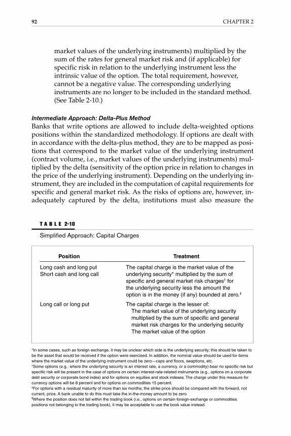
market values of the underlying instruments) multiplied by thesum of the rates for general market risk and (if applicable) forspecific risk in relation to the underlying instrument less theintrinsic value of the option. The total requirement, however,cannot be a negative value. The corresponding underlyinginstruments are no longer to be included in the standard method.(See Table 2-10.)

Intermediate Approach: Delta-Plus MethodBanks that write options are allowed to include delta-weighted optionspositions within the standardized methodology. If options are dealt within accordance with the delta-plus method, they are to be mapped as posi-tions that correspond to the market value of the underlying instrument(contract volume, i.e., market values of the underlying instruments) mul-tiplied by the delta (sensitivity of the option price in relation to changes inthe price of the underlying instrument). Depending on the underlying in-strument, they are included in the computation of capital requirements forspecific and general market risk. As the risks of options are, however, in-adequately captured by the delta, institutions must also measure the

92 CHAPTER 2

T A B L E 2-10

Simplified Approach: Capital Charges

Position Treatment

Long cash and long put The capital charge is the market value of theShort cash and long call underlying security* multiplied by the sum of

specific and general market risk charges† forthe underlying security less the amount theoption is in the money (if any) bounded at zero.‡

Long call or long put The capital charge is the lesser of:The market value of the underlying securitymultiplied by the sum of specific and generalmarket risk charges for the underlying securityThe market value of the option

*In some cases, such as foreign exchange, it may be unclear which side is the underlying security; this should be taken tobe the asset that would be received if the option were exercised. In addition, the nominal value should be used for itemswhere the market value of the underlying instrument could be zero—caps and floors, swaptions, etc.†Some options (e.g., where the underlying security is an interest rate, a currency, or a commodity) bear no specific risk butspecific risk will be present in the case of options on certain interest-rate-related instruments (e.g., options on a corporatedebt security or corporate bond index) and for options on equities and stock indexes. The charge under this measure forcurrency options will be 8 percent and for options on commodities 15 percent.‡For options with a residual maturity of more than six months, the strike price should be compared with the forward, notcurrent, price. A bank unable to do this must take the in-the-money amount to be zero.¶Where the position does not fall within the trading book (i.e., options on certain foreign-exchange or commoditiespositions not belonging to the trading book), it may be acceptable to use the book value instead.


gamma risk (risk resulting from nonlinear relationships between optionprice changes and changes in the underlying instrument) and vega risk(risk resulting from the sensitivity of the option price to fluctuations ofvolatility of the underlying instrument).

• Delta risk. Capital requirements for delta risk on options withinterest-rate instruments, equities, foreign exchange, andcommodities are based on the delta-weighted positions.

In computing the general market risk, delta-weighted options ondebentures or interest rates are allocated to the time bands for interest-rateinstruments and (if applicable) also for computing specific risk. Optionson derivatives are to be mapped twice, like the corresponding derivativesthemselves. Thus, an April purchase of a June call option on a three-monthinterest-rate future—on the basis of its delta equivalent—will be consid-ered as a long position with a maturity of five months and as a short posi-tion with a maturity of two months. The written option will similarly beentered as a long position with a maturity of two months and a short po-sition with a maturity of five months.

Options on equities, foreign exchange, gold, and commodities will alsobe incorporated into the measurement values as delta-weighted positions.

• Gamma risk. For each individual option, a gamma effect, asdefined here, is to be computed:

Gamma effect = 0.5 ⋅ γ ⋅ δ2 (2.10)

where γ designates gamma and δ the change in the underlyingvalue of the option. δ is computed by multiplying the marketvalue of the (notional) underlying value (contract volume, i.e.,amount receivable of the underlying value or nominal value) bythe following factors:

Interest-rate options: risk weight in accordance with Table 2-4[dependent on the maturity of the (notional) underlyinginstrument]Options on equities or stock indexes: 8 percentOptions on foreign exchange or gold: 10 percentOptions on commodities: 20 percent

A net gamma effect is to be computed from the gamma effects for thesame categories of underlying instruments. The individual categories aredefined as follows:

• Interest-rate instruments of the same currency and the same timeband

Market Risk 93


• Equities and stock indexes of the same national market or thesame currency zone

• Foreign currencies of each identical currency pair• Gold• Commodities

Only the negative net gamma effects are to be included in the com-putation of required equity and to be summed as absolute values to arriveat the total capital requirement.

The method of computing the gamma capital requirements pre-sented here takes into account only general market risk. Banks that pos-sess significant positions in options on specific equities or debtinstruments must, however, take specific risks into consideration in com-puting gamma effects.

• Vega risk. For each individual option, a vega effect, as definedhere, is to be computed:

Vega effect = 0.25 ⋅ ν ⋅ volatility (2.11)

where ν designates the value of vega.

For each category of underlying instruments, a net vega effect is tobe computed by addition of all vega effects of long positions (purchasedoptions) and subtraction of all vega effects of short positions (sold op-tions). The total capital requirements for the vega risk subject to a capitalcharge result from the aggregation of the sum of absolute values of netvega effects computed for each category.

The computation of vega effects is to be made based on implicitvolatilities. In the case of illiquid underlying instruments, other methodsmay be used on an exception basis to determine the volatility structure.

Intermediate Approach: Scenario MethodMore sophisticated banks also have the right to base the market risk capi-tal charge for options portfolios and associated hedging positions on sce-nario matrix analysis. This is accomplished by specifying a fixed range ofchanges in the option portfolio’s risk factors and calculating changes inthe value of the option portfolio at various points along this grid. For thepurpose of calculating the capital charge, the bank revalues the optionportfolio using matrices for simultaneous changes in the option’s under-lying rate or price and in the volatility of that rate or price. A different ma-trix is set up for each individual underlying instrument, as previouslydefined. As an alternative, at the discretion of each national authority,banks that are significant traders in options are permitted to base the cal-culation for interest-rate options on a minimum of six sets of time bands.

94 CHAPTER 2


When using this method, no more than three time bands should be com-bined into any one set.

In computing the capital requirements for options and related hedgingpositions using scenario analysis, the potential change in value for all possi-ble combinations of changes in the underlying instrument or rate (dimension1) and volatility (dimension 2), within the framework of a separate standardmatrix, is to be computed for each category of underlying instruments orrates.94 In the case of interest-rate instruments, it is possible to carry out a sep-arate analysis not for the instruments of each time band but to summarize thetime bands into groups. However, a maximum of three time bands maygrouped together, and at least six different groups must be formed. Forforeign-exchange options in the scenario definition, the arbitrage relation-ship between the underlying instruments may be taken into consideration.In such cases, the scenarios can be defined uniformly against the U.S. dollar.

The dimensions of the matrices to be used are defined as follows:

• Change in value of underlying instrument or rate (dimension 1). Thecomputations are to be made within the range for at least sevendifferent changes in value (including a change of 0 percent),where the assumed changes in value are at equally spacedintervals. The ranges are to be defined as follows:Interest-rate options: Plus or minus the change in yield, inaccordance with Table 2-6. Should several time bands beregrouped, the highest of the rates of the regrouped time bandsshall apply for the group.Options on equities and stock indexes: �8 percent.Options on foreign exchange and gold: �10 percent.Options on commodities: �20 percent.Computations on the basis of these value changes take into accountonly general market risk, not specific risk. The requirement forspecific risk is thus to be computed separately, based on the delta-weighted positions (cf. secs. 1.2 and 1.3 of the 1996 amendment).

• Change in volatility (dimension 2). In regard to the variation involatility, computations are to be conducted for at least threepoints: an unchanged volatility as well as relative changes involatility of �25 percent each.

After the computation of the matrix, each cell contains the net gainor loss of options and related hedging positions. The capital requirementcomputed for each category of underlying instrument corresponds in thiscase to the greatest of the losses contained in the matrix.

The scenario analysis is to be made based upon implicit volatilities.In the case of illiquid underlying instruments, other methods may be usedon an exception basis to determine the volatility structure.

Market Risk 95


2.7.7 Criticisms of the Standard Approach

Although the standard approach aims to identify banks with unusual ex-posure, it is still beset by problems, such as duration, diversification, inter-dependencies of market risk and credit risk, and qualitative requirements.

• The duration of some instruments cannot be easily identified.Mortgages, for instance, contain prepayment options that allowthe homeowner to refinance the loan if interest rates fall.Conversely, homeowners will make payments over a longerperiod if interest rates increase. The effective duration ofmortgages thus changes with the level of interest rates and thehistory of prepayments for a mortgage pool. Assigning a durationband to one of these instruments becomes highly questionable.More generally, the risk classification is arbitrary. The capitalcharges of 8 percent are applied uniformly to equities andcurrencies (and gold) without regard for their actual returnvolatilities.

• The standard approach does not account for diversification acrossrisks. Low correlations imply that the risk of a portfolio can bemuch less than the sum of individual component risks. Thisdiversification effect applies across market risks or acrossdifferent types of financial risks. Diversification across marketrisks is the easiest to measure. Historical data are available; theyreveal that correlations across sources of risk generatediversification and lower the total risk. These diversificationbenefits are not recognized by simply aggregating across riskfactors. Similarly, exchange movements are not perfectlycorrelated, nor are movements between interest rates andexchange rates. Assuming perfect correlations across varioustypes of risks overestimates portfolio risk and leads to capitaladequacy requirements that are too high.

• Correlations across different types of risks are more difficult todeal with. Most notably, default risk may be related to interest-rate risk. This is true for most floating-rate instruments (such asadjustable-rate mortgages, where borrowers may default shouldinterest rates increase to insufferable amounts).

• At times, even credit rating agencies have overlooked the effectof market risk on the possibility of default. A prime example isthe Orange County bankruptcy in December 1994. At thattime, S&P’s and Moody’s long-term credit ratings for thecounty were close to the highest possible—AA and Aa1,respectively—in spite of more than $1 billion in unrealizedlosses in the investment pool. The agencies claimed to have

96 CHAPTER 2


conducted a thorough examination of the county’s finances,yet they remained unaware of the impending cash crisis. Thisoccurred because the agencies focused only on credit risk—thatis, the possibility that a borrower could fail to repay. Therating agencies failed to recognize that market risk can lead tocredit risk.

2.8 THE INTERNAL MODEL APPROACH

In April 1995, the Basel Committee presented a major extension of themarket risk models.95 For the first time, it gave banks the option of usingtheir own risk measurement models to determine their capital charge.This decision stemmed from a recognition that many banks have devel-oped sophisticated risk management systems, in many cases far morecomplex than can be dictated by regulators. As for institutions lagging be-hind the times, this proposal provided a further impetus to create soundrisk management systems.

To use this approach, banks have to satisfy various qualitative re-quirements, including regular review by various management levelswithin the bank and by regulators.

To summarize, the general market risk charge on any day t is:

MRCt = max �k − ⋅ �60

i = 1

VaR t − i, VaR t − 1� (2.12)

where k is the multiplication factor determined by the supervisory au-thority, which can be set higher than its minimum of 3 if the supervisor isnot satisfied with the bank’s internal risk model.

To obtain total capital adequacy requirements, banks add their creditrisk charges to their market risk charges applied to trading operations.Upon application, the local supervisory authority can authorize an insti-tution to compute the capital requirements for market risks by means ofrisk aggregation models specific to each institution.

Risk aggregation models are statistical processes used to determinethe potential changes in the value of portfolios on the basis of changes inthe factors that determine such risks. In this connection, value at risk (VaR)is defined as that value which represents the maximum potential changein value of the total position, given a certain confidence level during a pre-determined period of time.

The equity requirements for interest-rate and equity price risks in thetrading book, and for foreign-exchange and commodity risks throughoutan institution, result from the aggregation of VaR-based capital chargesand any applicable additional requirements for specific risks on equityand interest-rate instruments.

1�60

Market Risk 97


2.8.1 Conditions for and Process of Granting Approval

Should an institution desire to apply the model-based approach, it shouldmake application to the local supervisory authority and submit documen-tation demanded by that authority.

The local supervisory authority shall base its decision concerningits consent to use the model-based approach on the results of testingconducted under its aegis together with the banking law auditors. Fur-thermore, the local supervisory authority can base its decision on the re-view results of foreign supervisory authorities, other banking lawauditors aside from those of the applicant, or other independent profes-sional experts.

The approval to use the model-based approach is dependent on cer-tain conditions.

The costs associated with testing the model during the preapprovalphase, as well as any subsequent necessary testing, are to be borne by theinstitution.

The local supervisory authority shall grant approval for the use ofthe model-based approach only if the following conditions have been meton a continual basis:

• The institution possesses a sufficient number of staff who arefamiliar with complex models not only in the area of trading, butalso in risk control, internal auditing, and back-office functions.

• The areas of trading, back office, and risk control possess anadequate electronic data processing (EDP) infrastructure.

• The risk aggregation model, in relation to the specific activities ofthe institution (composition of its trading book and its role withinthe individual markets—market maker, dealer, or end user), isconstructed on a sound concept and is correctly implemented.

• The preciseness of measurement of the risk aggregation model isadequate.

The local supervisory authority can demand that the risk aggrega-tion model first be monitored during a specific time frame and testedunder real-time conditions before it is implemented for the computationof capital requirements for market risks to ensure that the following con-ditions are met:

• The risk factors set as minimum requirements are taken accountof by the risk aggregation model.

• The risk aggregation model corresponds to the set minimumquantitative requirements.

• The set minimum qualitative requirements are complied with.

98 CHAPTER 2


After granting approval for the use of the model-based approach,the local supervisory authority is to be notified whenever:

• Significant modifications are made to the risk aggregation model.• The risk policy is changed.

The local supervisory authority shall decide whether and which fur-ther verification is necessary.

2.8.2 VaR-Based Components and Multiplication Factor

The internal model proposal is based on the following approach:

• The computation of VaR shall be based on a set of uniformquantitative inputs.

• A horizon of 10 trading days, or two calendar weeks, shall beused.

• A 99 percent confidence interval is required.• An observation period based on at least a year of historical data

and updated at least once a quarter shall be used.• Correlations can be recognized in broad categories (such as fixed

income) as well as across categories (e.g., between fixed incomeand currencies). As discussed before, this is an improvement overprevious proposals.

The capital charge shall be set as the higher of the previous day’sVaR or the average VaR over the last 60 business days, times a multiplica-tion factor. The exact value of this factor is to be determined by the localregulators, subject to an absolute floor of 3. This factor is intended to pro-vide additional protection against environments that are much less stablethan historical data would lead one to believe.

A penalty component shall be added to the multiplication factor ifbacktesting reveals that the bank’s internal model incorrectly forecastsrisks. The purpose of this factor is to give incentives to banks to improvethe predictive accuracy of the models and to avoid overly optimistic pro-jections of profits and losses due to model fitting. As the penalty factormay depend on the quality of internal controls at the bank, this system isdesigned to reward internal monitoring, as well as to develop sound riskmanagement systems.

The VaR-based equity requirement on a certain day corresponds tothe greater of the following two amounts:

• The VaR computed within the framework of the model-basedapproach for the portfolio held on the preceding day

Market Risk 99


• The average of the daily VaR values computed using the model-based approach for the preceding 60 trading days multiplied bythe multiplication factor for the specific institution as fixed by thelocal supervisory authority.

The multiplication factor for each specific institution shall be at least3. Its precise size will depend on the following:

• The fulfillment of the qualitative minimum requirements• The preciseness of forecasting by the risk aggregation model,

which is to be tested using so-called backtesting

2.8.3 Requirement for Specific Risks

Institutions that model specific risks neither in the form of residual risksnor in the form of event and default risks shall determine capital require-ments for specific risks in accordance with the standard approach.

Institutions that model specific risks in accordance with the prereq-uisites, but which in doing so limit themselves to capturing residual risks,and do not capture event and default risks at all or only partially, are sub-ject to additional capital requirements for the specific risks of equity andinterest-rate instruments. At the discretion of the institution, these may bedetermined using one of the following two approaches:

• Amount of VaR for equity and interest-rate portfolios• Amount of VaR for the specific risks inherent in the equity and

interest-rate portfolio

To determine the additional requirements, the amount of specificrisk captured by the risk aggregation model for equity or interest-rateportfolio shall, in this case, correspond to one of the following:

• The increase in VaR for the related subportfolio caused by theinclusion of specific risks

• The difference between the VaR for the related portfolio and theVaR, which ensues when all positions are substituted by positionswhose fluctuation in value is determined exclusively throughfluctuations of share market index or the reference interest-ratecurve

• The result of the analytical separation of general market risk fromspecific risk within the framework of a certain model

For the purposes of determining these additional capital require-ments, the general market risk for equities is to be defined by means of asingle risk factor: a representative market index or the first factor or a lin-ear combination of factors for the purposes of an empirical factor model.

100 CHAPTER 2


For interest-rate instruments, the general market risk shall correspond tothe fluctuation of the reference curve per currency based upon an estab-lished liquid market.

The institution must opt for a method for determining the additionalrequirements for specific risks and apply this method on a continual basis.

Should an institution provide the local supervisory authority withevidence that not only residual risks but also event and default risks arefully modeled, it may be dispensed from additional capital requirementsfor specific risks.

2.8.4 Combination of Model-Based and Standard Approaches

Institutions wishing to use internal models must in principle possess arisk aggregation model which, at minimum, covers all risk factor cate-gories (foreign exchange, interest rates, equity prices, and commodityprices) with respect to general market risks.

During the phase when an institution is migrating to the model-based approach, the local regulator can allow it to combine the model-based and standard approaches under the condition that the sameapproach is applied within the same risk factor category, i.e., either themodel-based or standard approach.

If positions in a certain risk factor category (such as commoditiesrisk) are absolute and insignificant when considered relatively, the localregulator may also allow an institution not to integrate these into themodel-based approach, but to deal with them separately in accordancewith the standard approach.

If the model-based and standard approaches are combined, the totalcapital requirement for market risks is arrived at through a simple addi-tion of the capital requirements for each component.

2.8.5 Specification of Market Risk Factors to Be Captured

An important part of a bank’s internal market risk measurement system isthe specification of an appropriate set of market risk factors, i.e., the mar-ket rates and prices that affect the value of the bank’s trading positions.The risk factors contained in a market risk measurement system should besufficient to capture the risks inherent in the bank’s portfolio of on- andoff-balance-sheet trading positions. Although banks will have some dis-cretion in specifying the risk factors for their internal models, the follow-ing guidelines should be fulfilled.

In principle, the risk aggregation model must take into considerationall risk factors that impact the relevant positions of the institution. An ex-

Market Risk 101


ception exists for the specific risks of equity and interest-rate instrumentswhose capital requirements may also be computed in accordance with thestandard approach.

The following minimum requirements apply for the individual riskfactor categories:

• Interest-rate risks. The interest-structure risks in each currency inwhich notable interest-rate-sensitive positions are held are to becaptured. In this respect, the following shall apply:The modeling of the interest maturity structure is to be made inaccordance with a recognized method.The number and distribution of the time bands must be appropriateto the size and structure of operations; there must be six at aminimum.The risk aggregation model must capture spread risks. Theseexist in that changes in value of cash flows with similar maturityand currency but issuers of different rating categories are notfully correlated.

• Foreign-exchange risks. Risk factors for the exchange ratesbetween the domestic currency and each foreign currency inwhich the institution holds a significant exposure are to be takeninto consideration.

• Equity price risks. The risk aggregation model must take intoconsideration a risk factor (e.g., a stock market index) at least foreach national market or single currency zone in which significantpositions are held. Risk factor definitions based on sector orbranch indexes are also possible.

• Commodities risks. Risk factors are to be modeled for each groupof commodities. In addition, the risk aggregation model musttake into consideration risks in the form of so-called convenienceyields—i.e., different developments in spot and forward pricesnot induced by interest rates.

• Risks of option positions. For options, the VaR measure, inaddition to delta risks, must capture at least the following risks:Gamma risks. Risks arising from nonlinear relationships betweenoption price changes and changes in the price of the underlyinginstrument.Vega risks. Risks arising from the sensitivity of option pricesagainst changes in volatility of the underlying instrument.Institutions with large and complex option portfolios must takeappropriate account of volatility risks of option positionsaccording to different maturities.

102 CHAPTER 2


• Specific risks of equity and interest-rate instruments. Specific risksequate those parts of aggregate volatility which relate tooccurrences in connection with the issuer of the individualinstruments and which cannot be explained by general marketrisks. To determine the capital requirements, the followingfurther differentiation is to be made:Specific risks in the form of residual risks. A residual risk representsthat part of the volatility of price fluctuations of equity andinterest-rate instruments which cannot be explained empiricallyby general market factors within the context of a single- ormultiple-factor model.Specific risks in the form of event and default risks. Specific eventrisks correspond to the risk that the price of a certain equity orinterest-rate instrument changes abruptly as a result ofoccurrences in connection with the issuer and to an extent whichcannot be explained as a general rule by the analysis of historicprice fluctuations. In addition to default risk, any abrupt pricefluctuations in connection with shocklike occurrences—such as,for instance, a takeover bid—constitute event risks.

An appropriate modeling of specific risks in the form of residualrisks presupposes that the model satisfies all quantitative and qualitativeminimum requirements, as well as that the following conditions are met:

• The historic change in the portfolio value is explained to a largedegree.

• The model demonstrably captures concentrations; i.e., it issensitive to fluctuations in the composition of the portfolio.

• The model has proven itself to be robust even in periods ofstrained market situations.

A complete capture of specific risks presupposes that residual risks aswell as event and default risks are captured by the risk aggregation model.

2.8.6 Minimum Quantitative Requirements

No specific type of risk aggregation model is prescribed for the determina-tion of capital requirements for market risks. Institutions may determinethe VaR on the basis of variance-covariance models, historical simulations,Monte Carlo simulations, and the like. The risk aggregation model, how-ever, must fulfill the following quantitative minimum requirements:

• Periodicity of computation. The VaR is to be computed daily onthe basis of the prior day’s positions.

Market Risk 103


• Confidence level. The computation of VaR should be effectedusing a one-tailed forecasting interval with a confidence level of99 percent.

• Holding period. In computing VaR, a change in the risk factorscorresponding to a change over a 10-day period is to be used.Also allowed are VaR numbers which are, for instance,determined on the basis of a holding period of 1 day andconverted to a value corresponding to a holding period of 10days by multiplication by 10. Institutions with significant optionpositions must, however, convert in due course to capturing inthe risk aggregation model the nonlinear relationship betweenoption price changes and changes in the price of thecorresponding underlying instrument by means of 10-daychanges in risk factors.

• Historical observation period and updating of data sets. Theobservation period for the forecasting of future changes andvolatilities in risk factors, including the correlation betweenthem which is at the basis of the VaR computation, must amountto one year at least. Should the individual daily observations betaken into consideration with individual weights in thecomputation of volatility and correlations (weighting), theweighted average observation period (weighted lag) must be atleast six months (i.e., the individual values in the weightedaverage must be at least six months old). The data sets must beupdated at least each quarter unless market conditions requireimmediate updating.

• Correlations. The VaR computation may be effected byrecognizing empirical correlations both within the general riskfactor categories (i.e., interest rates, exchange rates, equity prices,and commodity prices, including related volatilities) and betweenthe risk factor categories in case the correlation system of theinstitution is based on sound concepts and correctlyimplemented. The correlations are to be continuously monitoredwith particular care. Above all, the impact on the VaR of abruptchanges in correlations between the risk factor categories are tobe computed and evaluated regularly during stress testing.Should the computation of VaR be effected without consideringempirical correlations between the general risk factor categories,the VaR for the individual risk factor categories is to beaggregated through addition.

Alan Greenspan was very explicit about stress testing, highlightingits importance in the context of liquidity and systemic risk:

104 CHAPTER 2


The use of internal models for risk analysis, and as the basis for regulatorycapital charges has become common so far as market risk is concerned.While the limits of models, and the importance of the assumptions that mustbe made to put them to use, have been reasonably well understood, those is-sues have been brought into sharp focus by the Asian crisis. For example,firms now appreciate more fully the importance of the tails of the probabil-ity distribution of the shocks and of the assumptions about the covariance ofprices charges. The use of stress tests, which address the implications of ex-treme scenarios, has properly increased.96

2.8.7 Minimum Qualitative Requirements

The supervisory authorities are able to assure themselves that banks usingmodels have market risk management systems that are conceptuallysound and that are implemented with integrity. Accordingly, the supervi-sory authorities have specified a number of qualitative criteria that bankshave to meet before they are permitted to use a models-based approach.The extent to which banks meet the qualitative criteria may influence thelevel at which supervisory authorities set the multiplication factor. Onlythose banks whose models are in full compliance with the qualitative cri-teria are eligible for application of the minimum multiplication factor.

2.8.7.1 Integrity of DataThe institution shall demonstrate that it possesses sound, documented, in-ternally tested, and approved procedures which ensure that all transac-tions are captured, valued, and prepared for risk measurement in acomplete, accurate, and timely manner. Manual corrections to data are tobe documented so that the reason and exact content of the correction maybe reconstructed. In particular, the following principles shall apply:

• All transactions are to be confirmed daily with the counterparty.The confirmation of transactions as well as their reconciliation isto be effected by a unit independent of the trading department.Differences are to be investigated at once.

• A procedure must be in force which will ensure theappropriateness, uniformity, consistency, timeliness, andindependence of the data used in the valuation models.

• All positions are to be processed in a manner which ensurescomplete recording in terms of risk.

2.8.7.2 Independent Risk Control DepartmentThe institution must possess a risk control department which has quali-fied employees in sufficient number, is independent of the trading activi-

Market Risk 105


ties, and reports directly to a member of the management team responsi-ble for risk control.

Risk control shall support the following functions in particular:

• Organization and implementation of risk monitoring systems(trading and control systems).

• Close control over daily operations (limits, profit and lossstatement, etc.) including measurement criteria for market risk.

• Daily VaR computations, analyses, controls, and reporting:Preparation of daily reports on the results of the risk aggregationmodel, as well as analyses of the results, including therelationship between VaR and trading limits.Daily reporting to the responsible member of management.

• Completion of regular backtesting.97

• Completion of regular stress testing.• Testing and authorization of risk aggregation models, valuation

models for computing the daily profit and loss statement, andmodels to generate input factors (e.g., yield-curve models).

• Ongoing review and updating of the documentation for the riskmonitoring system (trading and control systems).

2.8.7.3 ManagementThe following provisions shall apply to management for the purposes ofusing the model-based approach:

• The responsible member of management must be informeddirectly on a daily basis, and in an appropriate manner, of theresults of the risk aggregation model, and he or she shall subjectthese to a critical review.

• The responsible member of management who evaluates the dailyreports of the independent risk-monitoring department mustpossess the authority to reduce the positions of individual tradersas well as to reduce the overall risk exposure of the bank.

• The responsible member of management must be informedperiodically of the results of backtesting and stress testing by therisk control department, and he or she must subject these resultsto critical review.

2.8.7.4 Risk Aggregation Model, Daily Risk Management,and System of LimitsThe following principles shall apply for the relationship between the riskaggregation model, daily risk control, and limits:

106 CHAPTER 2


• The risk aggregation model must be closely integrated into dailyrisk control. In particular, its results must be an integral part ofthe planning, monitoring, and management of the market riskprofile of the institution.

• There must exist a clear and permanent relationship between theinternal trading limits and the VaR (as it is used to determinecapital requirements for market risks). The relationship must beknown by both dealers and management.

• The limits are to be reviewed regularly.• The procedures to be followed in case the limits are exceeded,

and any applicable sanctions, must be clearly defined anddocumented.

2.8.7.5 BacktestingAn institution using the model-based approach must possess regular,sound, documented, and internally tested procedures for backtesting. Inprinciple, backtesting serves the purpose of obtaining feedback on thequality and precision of the risk measurement system.

The process of backtesting retrospectively compares the trading in-come during a defined period of time with the dispersion area of tradingincome predicted by the risk aggregation model for that period. The goalof the process is to be able to state, within certain probabilities of error,whether the VaR determined by the risk aggregation model actually cov-ers 99 percent of the trading outcome. For reasons of statistical reliabilityof the assertions, the daily trading profits and the daily VaR are comparedover a longer observation period.

For the purposes of the model-based approach, a standardized back-testing process is required to determine the multiplier specific to the insti-tution. Regardless, institutions should also use backtesting on a lowerlevel than that of the global risk aggregation model—for example, for in-dividual risk factors or product categories—in order to investigate ques-tions regarding risk measurement. In this manner, parameters other thanthose of the standardized backtesting process can be used in backtesting.

Institutions which determine not only requirements for general marketrisks but also those for specific risks by means of a risk aggregation modelmust also possess procedures for backtesting which indicate the adequacy ofmodeling specific risks. In particular, separate backtesting is to be conductedfor subportfolios (equity and interest-bearing portfolios) containing specificrisks, and the results are to be analyzed and reported upon demand to thelocal supervisory authority as well as to the banking law auditors.

Backtesting is to be conducted with consideration given to the fol-lowing standards in order to determine the multiplication factor specificto the institution:

Market Risk 107


• The test must be based on the VaR computed for the daily marketrisk report. The only difference relates to the fact that a holdingperiod of 1 day, not 10 days, is subject to a capital charge.

• The decision whether backtesting should be carried out on thebasis of actual trading results (i.e., inclusive of results of intradaytrading and inclusive of commissions), trading results fromwhich these items have been eliminated, or hypothetical tradingresults determined by revaluation to market of the financialinstruments in the institution’s portfolio on the preceding day isleft, in principle, to each individual institution. The condition isthat the process may be declared to be sound, and the incomefigures used must not systemically distort the test outcome. Inaddition, a uniform process over the time period is to be applied;i.e., the institution is not free to change the backtestingmethodology without consulting the local supervisory authority.

• The sampling method applied is to be based on 250 priorobservations.

The daily VaR reported internally, as well as the trading result on theday of computation, are to be documented in a manner that is irreversibleand that may be inspected at any time by the local supervisory authorityand the banking law auditors.

The institution shall daily compare the trading result with the VaR com-puted for the day before. Cases in which a trading loss exceeds that of the cor-respondingVaRaredesignatedasexceptions.Thereviewanddocumentationof these exceptions (for observations for the 250 preceding trading days) is tobe undertaken at least each quarter. The result of this quarterly review is to bereported to the local supervisory authority and the banking law auditors.

The increase in the multiplication factor specific to the institutioncorresponds to the number of exceptions noted during the observation pe-riod of the preceding 250 trading days (Table 2-11). In the case of the in-crease of the multiplication factor dependent on backtesting, the localsupervisory authority can ignore individual exceptions if the institutiondemonstrates that the exception does not relate to an imprecise (forecast-ing quality) risk aggregation model.

If there are more than four exceptions for the relevant observationperiod before 250 observations are available, the local supervisory author-ity is to be notified immediately. From that day forward, the institutionmust compute VaR with an increased multiplier until the local supervi-sory authority has made a final decision.

If an institution-specific multiplication factor greater than 3 shouldbe set as a result of backtesting, it is expected that the origin of the impre-cise estimates of the risk aggregation model will be investigated and, ifpossible, eliminated. The setting of the multiplier to 4 requires a compul-

108 CHAPTER 2


sory rapid and careful review of the model. The shortcomings are to beeliminated swiftly. Otherwise, the conditions for using the model-basedapproach will be deemed violated.

A reduction of the multiplication factor by the local supervisory au-thority will ensue only if the institution can demonstrate that the error hasbeen remedied and that the revised model presents an appropriate fore-casting quality.

2.8.7.6 Stress TestingAn institution using the model-based approach must apply regular,sound, consistent, documented, and internally tested stress-testing proce-dures. Important goals of stress testing are to ascertain whether the equitycan absorb large potential losses and to derive possible corrective action.

The definition of meaningful stress scenarios is left, in principle, tothe individual institution. The following guidelines, however, shall apply:

• Scenarios which lead to extraordinary losses or which render thecontrol of risks difficult or impossible are to be considered.

• Scenarios with extreme changes in market risk factors and thecorrelation between these (arbitrarily set scenarios or historicscenarios corresponding to periods of significant marketturbulence) are to be applied.

• Scenarios specific to the institution which must be consideredparticularly grave in regard to the specific risk positions are to beapplied.

• The analyses must capture liquidity aspects of marketdisturbances in addition to extreme changes in market riskfactors and their intercorrelation.

Market Risk 109

T A B L E 2-11

Multiplication Factor Specific to the Institution

Number of Exceptions Increase in Multiplication Factor

4 or fewer 0.00

5 0.40

6 0.50

7 0.65

8 0.75

9 0.85

10 or more 1.00


• The risks of all positions are to be included in stress testing,especially option positions.

In addition to actual quantitative stress tests and analyses thereof,lines of responsibility must exist to ensure that the outcome of stress testingwill trigger the necessary measures:

• The results of stress testing must be periodically reviewed by theresponsible member of management and be reflected in thepolicy and limits that are set by management and the internalauthority for direction, supervision, and control.

• If certain weaknesses are uncovered through stress testing, stepsmust be taken immediately to deal with these risks appropriately(e.g., by hedging or by reduction of the risk exposure).

2.8.7.7 Criticisms of the Internal Model ApproachThe internal model approach has been highly welcomed and criticized atthe same time. This part of the accord has been severely criticized by theInternational Swaps and Derivatives Association (ISDA). In particular, themultiplication factor of 3 is viewed as too large. The ISDA showed that afactor of 1 would have provided enough capital to cover periods of globalturmoil, such as the 1987 stock market crash, the 1990 Gulf War, and the1992 European Monetary System (EMS) crisis. An even more serious criti-cism is that the method based on an internal VaR creates a capital require-ment that is generally higher than the standard model prescribed by theBasel Committee. Hence, the current approach provides a negative incen-tive to the development of internal risk models.

2.9 THE PRECOMMITMENT MODEL

The debate on the appropriate risk measurement system took anotherturn when the U.S. Federal Reserve Board proposed a precommitment ap-proach to bank regulation in 1995. Under this third alternative, the bankwould precommit to a maximum trading loss over a designated hori-zon. This loss would become the capital charge for market risk. The su-pervisor would then observe, after, say, a quarterly reporting period,whether trading losses exceeded the limit. If so, the bank would be pe-nalized, which might include a fine, regulatory discipline, or higher fu-ture capital charges. Violations of the limits would also bring publicscrutiny to the bank, which provides a further feedback mechanism forgood management.

The main advantage of this “incentive-compatible” approach is thatthe bank itself chooses its capital requirement. As Kupiec and O’Brienhave shown, this choice is made optimally in response to regulatorypenalties for violations.98 Regulators can then choose the penalty that willinduce appropriate behavior.

110 CHAPTER 2


This proposal was welcomed by the ISDA, which argued that thisapproach explicitly recognizes the links between risk management prac-tices and firm-selected deployment of capital. Critics, in contrast, pointedout that quarterly verification is very slow in comparison to the real-timedaily capital requirements of the Basel proposals. Others worried that dy-namic portfolio adjustments to avoid exceeding the maximum loss couldexacerbate market movements, in the same way that portfolio insurancesupposedly caused the crash of 1987.

2.10 COMPARISON OF APPROACHES

At this point, it is useful to compare the pros and cons of each method. Thefirst, the standard model method, is generally viewed as least adequatebecause of the following factors:

• Portfolio considerations. The model ignores diversification effectsacross sources of risk.

• Arbitrary capital charges. The capital charges are only looselyrelated to the actual volatility of each asset category. This candistort portfolio choices, as banks move away from assets forwhich the capital charge is abnormally high.

• Compliance costs. Given that many banks already runsophisticated risk measurement systems, the standard modelimposes a significant additional reporting burden.

The second method, the internal model, addresses all of these issues.It relies on the self-interest of banks to develop accurate risk managementsystems. Internal VaR systems measure the total portfolio risk of the bank,account for differences in asset volatilities, and impose only small addi-tional costs. In addition, regulatory requirements will automaticallyevolve at the same speed as risk measurement techniques, as new devel-opments will be automatically incorporated into internal VaRs.

Unfortunately, from the viewpoint of regulators, the internal modelstill has some drawbacks:

• Performance verification. Supervisors are supposed to monitorwhether internal VaRs indeed provide good estimates of futureprofits and losses in trading portfolios. As capital charges arebased on VaRs, there may be an incentive to artificially lower theVaR figure to lower capital requirements; thus, verification byregulators is important. The problem is that, even with a well-calibrated model, there will be instances when losses will exceedthe VaR by chance (e.g., 5 percent of the time using a 95 percentconfidence level). Unfortunately, long periods may be needed todistinguish between chance losses and model inaccuracies. Thisissue makes verification difficult.

Market Risk 111


• Endogenity of positions. The banks’ internal VaRs typicallymeasure risk over a short interval, such as a day. Extending thesenumbers to a 10-day trading period ignores the fact that positionswill change, especially in response to losses or unexpectedly highvolatility. Therefore, measures of long-horizon exposure ignoreefficient risk management procedures and controls. Perhaps thisis why the ISDA found that the current approach appeared tooconservative.

Note that these problems do not detract from the usefulness of VaRmodels for corporate risk management. From the viewpoint of regulators,however, the precommitment approach has much to recommend, becauseit automatically accounts for changing positions. In addition, the risk cov-erage level is endogenously chosen by the bank, in response to the penaltyfor failure, which creates fewer distortions in capital markets.

Unfortunately, all models suffer from a performance verificationproblem. The regulator can compare only ex post, or realized, performanceto ex ante estimates of risk or maximum loss. Unless the maximum loss isset extremely high, there always will be instances in which a loss will ex-ceed the limit even with the correct model. The key then for regulators isto separate good intentions and bad luck from reckless behavior.

2.11 REVISION AND MODIFICATION OF THEBASEL ACCORD ON MARKET RISKS

2.11.1 The E.U. Capital Adequacy Directive

The history of capital adequacy requirements in Europe must be put in theperspective of plodding movements toward European economic and po-litical integration. The Single European Act of 1985 committed membercountries to achieving a free market in goods, services, capital, and labor.To this end, the European Union’s Investment Services Directive (ISD),which came into effect on January 1, 1996, swept away restrictions againstnonlocal financial services. Up until then, a securities firm that wanted todo business in another European Union country had to abide by localrules—for instance, having to establish separately capitalized subsidiaries(and expensive offices) in foreign countries. In effect, this raised the cost ofdoing business abroad and made Europe’s internal market less efficientthan it might otherwise have been.99

Under the new regulations, firms based in one E.U. country were au-thorized to carry out business in any other E.U. country. This was ex-pected to lead to the general consolidation of office networks. Forinstance, Deutsche Bank announced that its global investment banking ac-tivities would be centralized in London. Also, the centralization of riskmanagement would provide for better control of financial risks. In addi-

112 CHAPTER 2


tion to efficiency gains, more competition was expected to drive downtransaction costs and increase the liquidity of European financial markets.

To discourage firms from rushing to set up shop in the country with thelowest level of regulations, however, the European Union adopted Europe-wide capital requirements known as the Capital Adequacy Directive (CAD I). The CAD, published in March 1993, laid down minimum levels ofcapital to be adopted for E.U. banks and securities houses by January 1996.

In many ways, the CAD paralleled the Basel guidelines. It extendedthe 1989 Solvency Ratio and Own Funds Directives, which were similar tothe 1988 Basel accord. The 1993 requirements were very similar and insome cases identical to those laid out in the 1993 Basel proposal. Theamendment to incorporate market risks led to the updated version, CADII (April 1997), which allowed all E.U. institutions to run their own VaRmodels for daily calculation.

There were some differences, however. First, the Basel guidelineswere aimed only at banks, not securities houses. Regulation of securitieshouses is concerned mainly with orderly liquidation, while bank regula-tors aim to prevent outright failure. Second, the CAD II guidelines wereput into effect in 1996, whereas the Basel rules became effective in 1998,which left a period during which European firms had to comply with aseparate set of guidelines.

2.11.2 New Capital Adequacy Framework to Replace the 1988 Accord

The market risk approaches remained unchanged.100 Refer back to the dis-cussion earlier in this chapter of the 1996 Amendment to the Capital Ac-cord to Incorporate Market Risks (Section 2.6), which outlines thequantitative approaches in detail.

2.12 REGULATION OF NONBANKS

In many ways, the regulation of nonbank financial intermediaries paral-lels that of banks. Each of these institutions must learn to deal effectivelywith similar sources of financial risk.

Also, there is a tendency for lines of business to become increasinglyblurred. Commercial banks have moved into trading securities and pro-vide some underwriting and insurance functions. The trading portfoliosof banks contain assets, liabilities, and derivatives that are no differentfrom those of securities houses. Therefore, trading portfolios are meas-ured at market values, while traditional banking items are still reported atbook value. With the trend toward securitization, however, more andmore assets (such as bank loans) have become liquid and tradable.

Market Risk 113


2.12.1 Pension Funds

Although pension funds are not subject to capital adequacy requirements,a number of similar restrictions govern defined-benefit plans. The currentU.S. regulatory framework was defined by the Employee Retirement In-come Security Act (ERISA) promulgated in 1974. Under ERISA, companiesare required to make contributions that are sufficient to provide coveragefor pension payments. In effect, the minimum capital is the present valueof future pension liabilities. The obligation to make up for unfunded liabil-ities parallels the obligation to maintain some minimal capital ratio. Also,asterisk weights are replaced by a looser provision of diversification and ofnot taking excessive risks, as defined under the “prudent man” rule.

As in the case of banking regulation, federal guarantees are providedto pensioners. In the United States, the Pension Benefit Guarantee Corpo-ration (PBGC), like the Federal Deposit Insurance Corporation (FDIC),charges an insurance premium and promises to cover defaults by corpo-rations. Other countries have similar systems, although most other coun-tries rely much more heavily on public pay-as-you-go schemes, in whichcontributions from current employees directly fund current retirees. TheUnited States, Britain, and the Netherlands are far more advanced in theirreliance on private pension funds. Public systems in countries afflicted bylarge government deficits can ill afford generous benefits to an increas-ingly aging population. As a result, private pension funds are likely totake on increasing importance all over the world. With those will come theneed for prudential regulation.

2.12.2 Insurance Companies

Regulation of insurance companies is globally less centralized than that ofother financial institutions, whose insurance is regulated at the nationallevel. In the United States, the insurance industry is regulated at the statelevel. As in the case of FDIC protection, insurance contracts are ultimatelycovered by a state guaranty association. State insurance regulators set na-tionwide standards through the National Association of Insurance Com-missioners (NAIC).

In December 1992, the NAIC announced new capital adequacy re-quirements for insurers. As in the case of the early 1988 Basel accord, thenew rules emphasized credit risk. For instance, no capital would beneeded to cover holdings of government bonds and just 0.5 percent formortgages, but 30 percent of the value of equities would have to be cov-ered. This ratio was much higher than the 8 percent ratio required forbanks, which some insurers claimed put them at a competitive disadvan-tage vis-à-vis other financial institutions that were increasingly branchingout into insurance products.

114 CHAPTER 2


In the European Union, insurance regulation parallels that of banks,with capital requirements, portfolio restrictions, and regulatory interven-tion in cases of violation. For life insurance companies, capital must ex-ceed 4 percent of mathematical reserves, computed as the present valuesof future premiums minus future death liabilities. For non-life insurancecompanies, capital must exceed the highest of about 17 percent of premi-ums charged for the current year and about 24 percent of annual settle-ments over the past three years.

2.12.3 Securities Firms

The regulation of securities firms is still evolving. Securities firms hold se-curities on the asset and liability sides (usually called long and short posi-tions) of their balance sheets. Regulators generally agree that someprudent reserve should be available to cover financial risks. There is noagreement, however, as to whether securities firms should hold capital tocover their net positions, consisting of assets minus liabilities, or theirgross positions, consisting of the sum of all long plus short positions.

The United States and Japan use the gross position approach, theUnited Kingdom uses the net position, and the Basel Committee and theEuropean Union consider a variant of both approaches. The EuropeanUnion, for instance, required firms to have equity equal to 2 percent oftheir gross positions plus 8 percent of their net positions as of 1996.

Dimson and Marsh compare the effectiveness of these approachesfor a sample of detailed holdings of British market makers.101 Comparingthe riskiness of the portfolio to various capital requirements, they showthat the net position approach, as required by the United Kingdom, dom-inates the E.U. and U.S. approaches, as it best approximates the actualportfolio risk. The net position approach comes closest to what portfoliotheory would suggest.

Although there are differences in the regulations of banks and secu-rities firms, capital requirements are likely to converge as banks and secu-rities firms increasingly compete in the same markets. Currently, the sameaccounting rules apply to the trading-book activities of banks and thetrading activities of securities firms. In the United States, the 1933 Glass-Steagall Act, which separates the commercial and investment bank func-tions, is slowly being chipped away. The 1933 act is widely viewed asobsolete and overly restrictive, especially in comparison with the univer-sal banking system prevalent in Europe. Cracks in the Glass-Steagall wallstarted to appear in 1989, when commercial banks were allowed to under-write stocks and bonds on a limited basis (although no more than 10 per-cent of their revenues could come from underwriting). Banks have alsobeen expanding into insurance products, such as annuities, although fur-ther expansion is being fiercely resisted by U.S. insurance companies.

Market Risk 115


More recently, VaR has been gaining prominence in the regulation ofsecurities firms. The Securities and Exchange Commission, the Commod-ity Futures Trading Commission, and six major Wall Street securitieshouses have entered an agreement to base capital requirements on VaRmethodology. An authoritative resource for counterparty risk manage-ment, published by the Counterparty Risk Management Policy Group(CRMPG) in June 1999, is improving counterparty risk management prac-tices. CRMPG was formed by a group of 12 parties in the aftermath of the1998 market turmoil to promote better industrywide counterparty marketand credit risk practices. As for the commercial banking system, VaR isbound to become a universally accepted benchmark.102

2.12.4 The Trend Toward Risk-Based Disclosures

In addition to deriving strategic benefits from risk measurement and man-agement, institutions can use their risk management systems to generatethe kinds of reports that regulators are seeking. Disclosure guidelines re-leased by the U.S. Securities and Exchange Commission (SEC) in 1997allow companies to use VaR-type measures to communicate informationabout market risk. While many companies may be interested in measur-ing the aggregate market risk of their underlying exposures and hedge in-struments for internal purposes, current regulations require only thedisclosure of market risk–sensitive instruments (e.g., derivative con-tracts). Disclosure of underlying exposures and other positions is encour-aged, but not required. Whether companies decide to report only therequired disclosures or to also include the encouraged disclosures, thesystems being used for internal risk measurement can be leveraged tomeet regulatory disclosure requirements.

2.12.5 Disclosure Requirements

SEC market risk disclosure requirements affect all companies reportingtheir financial results in the United States.103 These regulations apply to de-rivative commodity instruments, derivative financial instruments, andother financial instruments (investments, loans, structured notes, mort-gage-backed securities, indexed debt instruments, interest-only and princi-pal-only obligations, deposits, and other debt obligations) that are sensitiveto market risk, all of which are collectively called market risk–sensitive instruments.

The SEC requires that companies provide both quantitative andqualitative information about the market risk–sensitive instruments theyare using.104 Currently, the allowed alternatives for the reporting of quan-

116 CHAPTER 2


titative information include tabular summaries of contract fair values;measures of sensitivity to market rate changes; and VaR measures ex-pressing potential loss of earnings, cash flows, or fair values.

The New Basel Capital Accord has integrated disclosure require-ments as an integral part of the entire accord, across all risk factors:

The third pillar, market discipline, will encourage high disclosure standardsand enhance the role of market participants in encouraging banks to holdadequate capital. The Committee proposes to issue later this year [2001]guidance on public disclosure that will strengthen the capital framework.105

2.12.6 Encouraged Disclosures

Apart from setting requirements on market risk–sensitive instruments,the SEC encourages, but does not require, risk disclosures on instruments,positions, and transactions not covered by Item 305 of Regulation S-K andItem 9A of Form 20-F. Such instruments can include physically settledcommodity derivatives, commodity positions, cash flows from antici-pated transactions, and other financial instruments, such as insurancecontracts. The BIS emphasizes disclosure practices and requires that regu-lations on the disclosure of specific, relevant information regarding mar-ket, credit, and operational risk be enforced; thus, the banks become moretransparent.

In general, the reporting of the combined market risk of underlyingbusiness exposures and market risk–sensitive instruments should providea more accurate portrayal of a firm’s total risk profile than reporting formarket risk–sensitive instruments alone.

2.13 MARKET INSTRUMENTS AND CREDIT RISKS

Credit exposure and market risk are interrelated, and the boundaries be-tween credit and market risk increasingly overlap and merge; this is partic-ularly obvious in the case of credit risk derivatives. It can be argued thatcredit risk is a component of market risk, as it reflects the company- or issuer-specific risk. A change in the quality of a company and its ability tofulfill its financial obligations is, in an efficient market, immediately re-flected in the specific risk, either on the equity side through the idiosyncraticrisk or on the fixed-income side through the spread on top of the risk-freeterm structure. This reflects the balance sheet, as all financing instrumentsultimately lead back to the balance sheet of the original underlying com-pany and should therefore reflect the same company-specific risk.

Credit exposures from market-driven transactions such as swaps,forwards, and purchased options are an issue for all participants in the

Market Risk 117


OTC derivatives markets. Credit or market risk can result from fluctua-tions in market rates. (More instrument types are analyzed and decom-posed regarding market, credit, and operational risk in Chapter 3.)

In the case of a swap, the interrelationship of credit and market riskcan be illustrated in a simple example. Party A engages in an interest-rateswap with Party B, paying a five-year fixed rate and receiving a three-month LIBOR. If the five-year rate goes down, A incurs a market loss be-cause it agreed to pay B an above-market interest rate. On the other hand, ifa 10-year rate falls, the swap is in the money for A. However, this mark-to-market (MTM) gain on the swap is now a credit exposure to B—if B defaults,A forsakes the MTM gain on the swap. Therefore, a company has credit ex-posure whenever rates fluctuate in its favor. A company has potential creditexposure from the time a contract is initiated up to final settlement.

For example, simulating a simple equity-index fall would do little touncover the risk of a market-neutral risk arbitrage book. In a real-worldexample, Long Term Capital Management (LTCM) had leveraged credit-spread-tightening positions (i.e., long corporate bond positions were interest-rate hedged with short Treasuries) in August 1998. This portfoliowas supposedly market neutral.106

A stress test for spread widening (i.e., flight-to-safety phenomenon)would have uncovered the potential for extreme losses. Stressed marketsoften give rise to counterparty credit risk issues that may be much moresignificant than pure market impacts. For example, a market-neutral swapportfolio could result in huge credit exposures if interest rates moved sig-nificantly and counterparties defaulted on their contractual obligations.While market rates and creditworthiness are unrelated for small marketmovements, large market movements could precipitate credit events, andvice versa. Note that it is much more straightforward to reduce marketrisk than credit risk. To reduce the market risk in our example, Party A canpurchase a 10-year government bond or futures contract, or enter into anopposite swap transaction with another counterparty. Credit risk presentsa more complex problem. For example, taking an offsetting swap with an-other counterparty to reduce market risk actually increases credit risk (onecounterparty will always end up owing the party the net present value ofthe swap). Solutions to the credit problem are available, however. Party Acould arrange a credit enhancement structure with Party B, such as struc-turing a collateral or MTM agreement (e.g., Party B agrees to post collat-eral or pay the MTM of a swap on a periodic basis, or if a certain thresholdis reached). Furthermore, a credit derivative could be written by a thirdparty to insure the swap contract.

Options have their own credit and market risk profile (Figure 2-8).Only purchasers of options have credit exposure to their counterparts. Ifthe option is in the money and the counterparty defaults, the party is introuble. For example, Party A has potential credit exposure when it buys a

118 CHAPTER 2


put option on the S&P 500 Stock Index to insure an equity portfolio. If theequity market falls and Party A’s counterparty defaults on its obligation tohonor the put option, A would incur a credit loss (for example, if the in-surer of its equity portfolio does not fulfill its obligation). Sellers of op-tions do not have credit exposure. After a party sells an option and collectsthe premium, it is not exposed to its counterparty (for example, the coun-terparty will not owe it anything, but it will potentially owe something tothe counterparty). As a seller of options, a party incurs only market risk(i.e., the risk that market rates will move out of its favor). The projectedcredit exposure of options increases with time, with the peak exposure ex-pected just before final settlement.

The credit risk of swaps and forwards is mostly counterparty risk.Counterparties engaging in swaps and forwards incur credit exposure toeach other. Swaps and forwards are generally initiated at the money. Thatis, at the beginning of a contract, neither counterparty owes the other any-thing. However, as rates change, the MTM value of the contract changes,and one counterparty will always owe another counterparty money (theamount owed will be the MTM value).

Usually, the projected credit exposure of an interest-rate swap has aconcave shape. Projected exposure of a currency swap, however, increaseswith time and peaks just before settlement. A currency swap has a larger,and continually upward sloping, exposure profile due to the foreign-

Market Risk 119

Counterparty

TradingMiddle office /

risk control

Transaction

Settlementaccounting

DealConfirmation

Creditrisk

Marketrisk

Reconciliation

Reporting

Risk exposures

F I G U R E 2-8

Market, Credit, and Operational Risks from a Transaction Perspective.


exchange risk of the principal amount, which is exchanged only at finalsettlement. Projected credit exposure of a forward also slopes continuallyupward, as there is no exchange of payments before settlement.

2.14 SUMMARY

Market risk management has become a relatively mature discipline.Therefore, this chapter focuses on the evolution of the different mod-els and approaches, and on the conditions and assumptions which arelinked to those models and approaches. The groundbreaking works ofMarkowitz and Black and Scholes 50 years ago set the framework in themarket risk area, subsequently enhanced and modified by others. Theseorigins have shaped the profile of the discipline and provided a substan-tial set of specialized parameters and assumptions, typical for a disciplineconsidered to have an integrated framework. The terms time horizon, di-versification, and volatility, just to mention three parameters, have a differ-ent meaning within the market risk framework than in credit risk oroperational risk. The international regulatory body has developed the su-pervisory framework for each risk category independently from the othercategories, and tries to bring the individual components together in thenew capital adequacy framework.

The discussion of different models and their application within theregulatory framework covering market risk–related issues is a central partof this chapter. The Basel Committee on Banking Supervision of the Bankfor International Settlement has moved from a prescriptive approach onsupporting risk with capital to a risk-sensitive framework, and the latestapproach is intended to integrate the market, credit, and operational riskcategories into an integrated risk framework. This chapter focuses on theconceptual approaches regarding the modeling of market risk and the reg-ulatory initiatives on market risk and VaR.

2.15 NOTES

1. Bank for International Settlement (BIS), Basel Committee on BankingSupervision, Amendment to the Capital Accord to Incorporate Market Risks,Basel, Switzerland: Bank for International Settlement, January 1996, sec. I.1.p. 3.

2. Harry M. Markowitz, “Portfolio Selection (1),” Journal of Finance 7 (March1952), 77–91.

3. William Shakespeare, The Merchant of Venice, ca. 1596–1598, Antonio in act 1,scene 1.

4. J. R. Hicks, “A Suggestion for Simplifying the Theory of Money,” Economica(February 1935), 1–19.

5. Ibid., 7.

120 CHAPTER 2


6. James Tobin, “Liquidity Preference as Behavior Towards Risk,” Review ofEconomic Studies 26/1 (February 1958), 65–86.

7. J. R. Hicks, “Liquidity,” Economic Journal 72 (December 1962), 787–802.

8. Ibid.

9. J. Marschak, “Money and the Theory of Assets,” Econometrica 6 (1938),311–325.

10. Ibid., 314.


12. William F. Sharpe, “Capital Asset Prices: A Theory of Market EquilibriumUnder Conditions of Risk,” Journal of Finance 19/3 (September 1964),425–442; John Lintner, “The Valuation of Risk Assets and the Selection ofRisky Investments in Stock Portfolios and Capital Budgets,” Review ofEconomics and Statistics 47/1 (February 1965), 13–37.

13. Johnann von Neumann and Oskar Morgenstern, “Theory of Games andEconomic Behavior,” 3d ed., Princeton, NJ: Princeton University Press, 1967(1st ed., 1944).

14. J. B. Williams, The Theory of Investment Value, Cambridge, MA: HarvardUniversity Press, 1938.

15. J. L. Farrell, “The Dividend Discount Model: A Primer,” Financial AnalystsJournal 41 (November–December 1985), 16–19, 22–25.

16. D. H. Leavens, “Diversification of Investments,” Trusts and Estates 80 (May1945), 469–473.

17. Harry M. Markowitz, “Portfolio Selection (1),” Journal of Finance 7 (March1952), 77–91.

18. A. D. Roy, “Safety First and the Holding of Assets,” Econometrica 20/3 (July1952), 431–449.

19. Harry M. Markowitz, “The Optimization of a Quadratic Function Subject toLinear Constraints,” Naval Research Logistics Quarterly 3 (1956), 111–133;Portfolio Selection—Efficient Diversification of Investments, New York: JohnWiley & Sons, 1959; Mean-Variance Analysis in Portfolio Choice and CapitalMarkets, Oxford, U.K.: Basil Blackwell, 1987.

20. Harry M. Markowitz, Portfolio Selection (2), 2d ed., Oxford, U.K.: BasilBlackwell, 1992, p. 154ff.


22. William F. Sharpe, “Capital Asset Prices, A Theory of Market EquilibriumUnder Conditions of Risk,” Journal of Finance 19/3 (September 1964),425–442.

23. John Lintner, “The Valuation of Risk Assets and the Selection of RiskyInvestments in Stock Portfolios and Capital Budgets,” Review of Economicsand Statistics 47/1 (February 1965), 13–37; “Security Prices, Risk, andMaximal Gains from Diversification,” Journal of Finance 20 (1965), 587–615.

Market Risk 121


24. Jan Mossin, “Equilibrium in a Capital Asset Market,” Econometrica 35/4(October 1966), 768–783.

25. Diana R. Harrington, Modern Portfolio Theory, the Capital Asset Pricing Modeland Arbitrage Pricing Theory: A User’s Guide, 2d ed., Englewood Cliffs, NJ:Prentice-Hall, 1987, p. 35.

26. For a detailed discussion, see Christoph Aukenthaler, “Trust Banking,Theorie und Praxis des Anlagegeschäftes,” PhD thesis, University of Zurich,Haupt, Bern, 1991, 244ff., or Pirmin Hotz, “Das Capital Asset Pricing Modelund die Markteffizienzhypothese unter besonderer Berücksichtigung derempirisch beobachteten ‘Anomalien’ in den amerikanischen und andereninternationalen Aktienmärkten,” PhD thesis, University St. Gall, Victor HotzAG, Baar, 1989, p. 43ff.

27. Eugene Fama, “Efficient Capital Market: A Review of Theory and EmpiricalWork,” Journal of Finance 3 (1970), 383–417.

28. Thomas Vock and Heinz Zimmermann, “Risiken und Renditenschweizerischer Aktien,” Schweizerzische Zeitschrift für Volkwirtschaft undStatistik 4 (1984), 547–576.

29. Eugene Fama, Foundations of Finance, New York: Basic Books, 1976, p. 25ff.30. Stanley J. Kon, “Models of Stock Returns—A Comparison,” Journal of Finance

39 (1984), 147–165.31. Randolph Westerfield, “An Examination of Foreign Exchange Risk and

Fixed and Floating Exchange Rate Regimes,” Journal of InternationalEconomics 7 (1977), 181–200.

32. Walter Wasserfallen and Heinz Zimmermann, “The Behaviour of InterdailyExchange Rates,” Journal of Banking and Finance 9 (1985), 55–72.

33. Heinz Zimmermann, “Zeithorizont, Risiko und Performance, eineÜbersicht,” Finanzmarkt und Portfolio Management 2 (1991), 169.

34. Fischer Black, “Capital Market Equilibrium with Restricted Borrowing,”Journal of Business 7, 444–454.

35. For a detailed analysis see Fischer Black, Michael C. Jensen, and MyronScholes, “The Capital Asset Pricing Model: Some Empirical Tests,” inMichael Jensen, Studies in the Theory of Capital Markets, New York: Praeger,1972.

36. Eugene Fama, “Efficient Capital Market: A Review of Theory and EmpiricalWork,” Journal of Finance 3 (1970), 383–417; Fischer Black, Michael C. Jensen,and Myron Scholes, “The Capital Asset Pricing Model: Some EmpiricalTests,” in Michael Jensen, Studies in the Theory of Capital Markets, New York:Praeger, 1972; Eugene Fama and James MacBeth, “Risk, Return andEquilibrium: Empirical Tests,” Journal of Political Economy 9 (1973), 601–636.

37. Stephen A. Ross, “The Arbitrage Theory of Capital Asset Pricing,” Journal ofEconomic Theory 13 (1976), 341–360.

38. Louis Bachelier, “Theorie de la Speculation,” Annales de l’Ecole NormaleSuperieure 17 (1900), 21–86. English translation by A.J. Boness in Paul H.Cootner (ed.), The Random Character of Stock Market Prices, Cambridge, MA:MIT Press, 1967, pp. 17–78.

122 CHAPTER 2


39. C. Sprenkle, “Warrant Prices as Indicators of Expectations and Preferences,”Yale Economic Essays 1 (1961), 172–231; P. Samuelson, “Rational Theory ofWarrant Pricing,” Industrial Management Review 10 (1965), 15–31.

40. Fischer Black and Myron Scholes, “The Pricing of Options and CorporateLiabilities,” Journal of Political Economy 81 (May–June 1973), 637–654; R. C.Merton, “Theory of Rational Option Pricing,” Bell Journal of Economics andManagement Science 4/1 ( June 1974), 141–183.

41. Ibid., Black and Scholes.

42. Ibid., Merton.

43. Fischer Black, “The Pricing of Commodity Contracts,” Journal of FinancialEconomics 3 (1976), 167–179.

44. M. Asay, “A Note on the Design of Commodity Option Contracts,” Journal ofFinance 2 (1982), 1–8.

45. M. Garman and S. Kohlhagen, “Foreign Currency Option Values,” Journal ofInternational Money and Finance 2 (1983), 231–238.

46. R. Geske, “The Valuation of Compound Options,” Journal of FinancialEconomics 7 (1979), 63–81.

47. Richard Roll, “An Analytic Valuation Formula for Unprotected AmericanCall Options on Stocks with Known Dividends,” Journal of FinancialEconomics 5 (1977), 251–258; R. Geske, “A Note on an Analytical Formula forUnprotected American Call Options on Stocks with Known Dividends,”Journal of Financial Economics 7 (1979), 375–380; R. Whaley, “On the Valuationof American Call Options on Stocks with Known Dividends,” Journal ofFinancial Economics 9 (1981), 207–211.

48. M. Rubinstein, “Pay Now, Choose Later,” Risk (February 1991), 13.

49. S. Gray and R. Whaley, “Valuing S&P 500 Bear Market Warrants with aPeriodic Reset,” Journal of Derivatives 5 (1997), 99–106.

50. B. Goldman, H. Sosin, and M. Gatto, “Path Dependent Options: Buy at theLow, Sell at the High,” Journal of Finance 34 (1979), 1111–1127.

51. M. Rubinstein and E. Reiner, “Breaking Down the Barriers,” Risk (September1991), 31–35.

52. J. Cox, S. Ross, and M. Rubinstein, “Option Pricing: A Simplified Approach,”Journal of Financial Economics 7 (1979), 229–264; R. Rendleman Jr. and B.Bartter, “Two-State Option Pricing,” Journal of Finance 34 (1979), 1093–1110.

53. P. Boyle, J. Evnine, and S. Gibbs, “Numerical Evaluation of MultivariateContingent Claims,” Review of Financial Studies 2 (1989), 241–250.

54. P. Boyle, “A Lattice Framework for Option Pricing with Two StateVariables,” Journal of Financial and Quantitative Analysis 23 (1988), 1–12.

55. E. Schwartz, “The Valuation of Warrants: Implementing a New Approach,”Journal of Financial Economics 4 (1977), 79–93; M. Brennen and E. Schwartz, “TheValuation of American Put Options,” Journal of Finance 32 (1977), 449–462.

56. P. Boyle, “Options: A Monte Carlo Approach,” Journal of Financial Economics4 (1977), 323–338.

Market Risk 123


57. R. Geske and H. Johnson, “The American Put Valued Analytically,” Journal ofFinance 39 (1984), 1511–1524.

58. G. Barone-Adesi and R. Whaley, “Efficient Analytic Approximation ofAmerican Option Values,” Journal of Finance 42 (1987), 301–320.

59. L. MacMillan, “Analytic Approximation for the American Put Option,”Advances in Futures and Options Research 1 (1986), 119–139.

60. R. Merton, “Theory of Rational Option Pricing,” Bell Journal of Economics andManagement Science 4/1 (1973), 141–183.

61. J. Cox and S. Ross, “The Valuation of Options for Alternative StochasticProcesses,” Journal of Financial Economics 3 (1976), 145–166.

62. E. Derman and I. Kani, “Riding on the Smile,” Risk (July 1994), 32–39; D. Dupire, “Pricing with a Smile,” Risk (July 1994), 18–20; M. Rubinstein andE. Reiner, “Implied Binomial Trees,” Journal of Finance 49 (1994), 771–818.

63. R. C. Merton, “Option Pricing when Underlying Stock Returns areDiscontinuous,” Journal of Financial Economics 3 (1976), 125–143.

64. J. Hull and A. White, “The Pricing of Options and Assets with StochasticVolatilities,” Journal of Finance 42 (1987), 281–300.

65. L. Scott, “Option Pricing when the Variance Changes Randomly: TheoryEstimation, and an Application,” Journal of Financial and Quantitative Analysis22 (1987), 419–438; J. Wiggins, “Option Values Under Stochastic Volatility:Theory and Empirical Estimates,” Journal of Financial Economics 19 (1987),351–372.

66. D. Bates, “Jumps and Stochastic Volatility: Exchange Rate Processes Implicitin PHLX Deutschemark Options,” Review of Financial Studies 9 (1996), 69–108.

67. Alan Greenspan, “Measuring Financial Risk in the Twenty-First Century,”remarks before a conference sponsored by the Office of the Comptroller ofthe Currency, Washington, D.C., October 14, 1999.

68. Bank for International Settlement (BIS), Basel Committee on BankingSupervision, International Convergence of Capital Measurement and CapitalStandards, Basel, Switzerland: Bank for International Settlement, July 1988.

69. See U.S. General Accounting Office, Long-Term Capital Management,Regulators Need to Focus Greater Attention on Systemic Risk, Washington, DC:General Accounting Office, October 1999.

70. See the analysis and recommendations in Commodity Futures TradingCommission (CFTC), Hedge Funds, Leverage, and the Lessons of Long-TermCapital Management: Report of the President’s Working Group on FinancialMarkets, Washington, DC: Commodity Futures Trading Commission, April1999, www.cftc.gov/tm/hedgefundreport.html, accessed May 19, 2000.

71. Financial Times, “Greenspan Hits Out at Way Banks Treat Risk” (October 12,1999), 10.

72. The Basel Committee’s members are representatives of the central banks andlocal regulatory organizations of the Group of Ten (G-10) countries:Belgium, Canada, France, Germany, Italy, Japan, the Netherlands, Sweden,the United Kingdom, and the United States, plus Luxembourg and

124 CHAPTER 2


Switzerland. The committee meets four times a year, usually in Basel,Switzerland, under the chairmanship of the Bank for InternationalSettlement, where the permanent secretariat of the committee is located.

73. Bank for International Settlement (BIS), Basel Committee on BankingSupervision, International Convergence of Capital Measurement and CapitalStandards, Basel, Switzerland: Bank for International Settlement, July 1988.

74. Bank for International Settlement (BIS), Basel Committee on BankingSupervision, Prudential Supervision of Banks’ Derivatives Activities, Basel,Switzerland: Bank for International Settlement, December 1994; Amendmentto the Capital Accord of July 1988, Basel, Switzerland: Bank for InternationalSettlement, July 1994; Basel Capital Accord: The Treatment of the Credit RiskAssociated with Certain Off-Balance-Sheet Items, Basel, Switzerland: Bank forInternational Settlement, July 1994.

75. The U.S. banking industry regulators consist of the Federal Reserve Board,the Office of the Comptroller of the Currency, and the Federal DepositInsurance Corporation.

76. The Basel Committee has extended the add-ons on equities, precious metals,and commodities contracts and increased the add-ons in general for longermaturities. See Bank for International Settlement (BIS), Basel Committee onBanking Supervision, Treatment of Potential Exposure for Off-Balance-Sheet Items,Basel, Switzerland: Bank for International Settlement, April 1995. See as wellthe discussion of the Basel Committee’s 1994 and 1995 modifications inSection 2.8. See also the regulations issued in Bank for InternationalSettlement (BIS), Basel Committee on Banking Supervision, Interpretation of theCapital Accord for the Multilateral Netting of Forward Value Foreign ExchangeTransactions, Basel, Switzerland: Bank for International Settlement, April 1996;and Survey of Disclosures About Trading and Derivatives Activities of Banks andSecurities Firms: Joint Report by the Basel Committee on Banking Supervision andthe Technical Committee of the International Organisation of Securities Commission,Basel, Switzerland: Bank for International Settlement, November 1996.

77. Bank for International Settlement (BIS), Basel Committee on BankingSupervision, Amendment to the Capital Accord to Incorporate Market Risks,Basel, Switzerland: Bank for International Settlement, January 1996,modified in September 1997.

78. Ibid.

79. Committee members who are also members of the European Union regardthis definition as being consistent with (albeit less detailed than) thedefinition of the trading book in the EU’s Capital Adequacy Directive.

80. Bank for International Settlement (BIS), Basel Committee on BankingSupervision, Amendment to the Capital Accord to Incorporate Market Risks,Basel, Switzerland: Bank for International Settlement, January 1996,modified September 1997.

81. Ibid., para. II.a.

82. Bank for International Settlement (BIS), Basel Committee on BankingSupervision, The New Basel Capital Accord: Consultative Document, Issued for

Market Risk 125


Comment by 31 May 2001, Basel, Switzerland: Bank for InternationalSettlement, January 2001, part 2I, para. 20.

83. Bank for International Settlement (BIS), Basel Committee on BankingSupervision, Amendment to the Capital Accord to Incorporate Market Risks,Basel, Switzerland: Bank for International Settlement, January 1996,modified September 1997, para. 7.

84. Switzerland Federal Banking Commission, “Guidelines Governing CapitalAdequacy Requirements to Support Market Risks,” EG-FBC Circular No.97/1, October 22, 1997.

85. See comments in Reto R. Gallati, “De-Minimis-Regel diskriminiert,”Schweizer Bank (Zurich), 9 (1998), 41–43.

86. See definition of specific risk in Bank for International Settlement (BIS),Basel Committee on Banking Supervision, Amendment to the Capital Accord toIncorporate Market Risks, Basel, Switzerland: Bank for InternationalSettlement, January 1996, modified September 1997, para. I.b, footnote 5.

87. See Bank for International Settlement (BIS), Basel Committee on BankingSupervision, International Convergence of Capital Measurement and CapitalStandards, Basel, Switzerland: Bank for International Settlement, July 1988.

88. Traded mortgage securities and mortgage derivative products possessunique characteristics because of the risk of prepayment. Accordingly, forthe time being, no common treatment applies to these securities, which aredealt with at national discretion. A security that is the subject of arepurchase or securities-lending agreement will be treated as if it were stillowned by the lender of the security—i.e., it will be treated in the samemanner as other securities positions.

89. This includes the delta-equivalent value of options. The delta equivalent ofthe legs arising out of the treatment of caps and floors can also be offsetagainst each other under the rules laid down in this paragraph.

90. The separate legs of different swaps may also be matched, subject to thesame conditions.

91. Where equities are part of a forward contract, a future, or an option(quantity of equities to be received or to be delivered), any interest rate orforeign currency exposure from the other leg of the contract should bereported.

92. For example, an equity swap, in which a bank receives an amount based onthe change in value of one particular equity or stock index, and pays on adifferent index will be treated as a long position in the former and a shortposition in the latter. Where one of the legs involves receiving or paying afixed or floating interest rate, that exposure should be slotted into theappropriate repricing time band for interest-rate-related instruments. Thestock index should be covered by the equity treatment.

93. Bank for International Settlement (BIS), Basel Committee on BankingSupervision, Amendment to the Capital Accord to Incorporate Market Risks,Basel, Switzerland: Bank for International Settlement, January 1996,modified September 1997, sec. 5.3.1, para. 130.

126 CHAPTER 2


94. Ibid., sec. 5.3.2.b, para. 96.

95. Bank for International Settlement (BIS), Basel Committee on BankingSupervision, Proposal to Issue a Supplement to the Basel Capital Accord to CoverMarket Risks, Basel, Switzerland: Bank for International Settlement, April1995; An Internal Model–Based Approach to Market Risk Capital Requirements,Basel, Switzerland: Bank for International Settlement, 1995.

96. Alan Greenspan, “Risk Management in the Global Financial System—Beforethe Annual Financial Markets Conference of the Federal Reserve Bank ofAtlanta,” Miami Beach, Florida, February 27, 1998.

97. Bank for International Settlement (BIS), Basel Committee on BankingSupervision, Supervisory Framework for the Use of “Backtesting” in Conjunctionwith the Internal Models Approach to Market Risk Capital Requirements, Basel,Switzerland: Bank for International Settlement, January 1996.

98. P. Kupiec and J. O’Brien, “A Pre-Commitment Approach to CapitalRequirements for Market Risk,” FEDS Working Paper no. 95-34,Washington, DC: Federal Reserve Board of Governors, 1995.

99. A typical management response is to cut positions as losses accumulate.This pattern of trading can be compared to portfolio insurance, whichattempts to replicate a put option. Therefore, attempts by management tocontrol losses will create a pattern of payoffs over long horizons that will beasymmetrical, similar to options. The problem is that traditional VaRmeasures are inadequate with highly nonlinear payoffs.

100. Bank for International Settlement (BIS), Basel Committee on BankingSupervision, The New Basel Capital Accord: Consultative Document, Issued forComment by 31 May 2001, Basel, Switzerland: Bank for InternationalSettlement, January 2001, 6ff.; Amendment to the Capital Accord to IncorporateMarket Risks, Basel, Switzerland: Bank for International Settlement, January1996, modified September 1997.

101. E. Dimson and R. Marsh, “Capital Requirements for Securities Firms,”Journal of Finance 50 (1995), 821–851.

102. Misconceptions of models are that they are conceptually built for “normalconditions”. See comments from Tim Shepheard-Walwyn and RobertLitterman, “Building a Coherent Risk Measurement and CapitalOptimization Model for Financial Firms,” paper presented at theConference on Financial Services at the Crossroads: Capital Regulation inthe 21st Century, New York, February 26–27, 1998, FRBNY Economic PolicyReview (October 1998), 173ff. and Section 5.8 of this book, which discussesmisconceptions of models.

103. See Securities and Exchange Commission Item 305 of Regulation S-K andItem 9A of Form 20-F.

104. For a description of the required qualitative market risk disclosures, seeSecurities and Exchange Commission Item 305(b) of Regulation S-K andItem 9A(b) of Form 20-F.

105. Bank for International Settlement (BIS), Basel Committee on BankingSupervision, The New Basel Capital Accord: Consultative Document, Issued for

Market Risk 127


Comment by 31 May 2001, Basel, Switzerland: Bank for InternationalSettlement, January 2001, paras. 74, 655ff.

106. A market-neutral risk arbitrage book would consist of a series of long andshort positions; this hedges out market risk but leaves exposure to firm-specific risk. A trading strategy that eliminates broad market risk (equity,interest rate, foreign exchange, or commodity) leaves only residual risk. Forexample, a hedge fund manager can hedge the market risk of a U.S. stockportfolio by shorting S&P 500 Stock Index futures, leaving only firm-specificresidual risk.

128 CHAPTER 2


C H A P T E R 3

Credit Risk

3.1 BACKGROUND

Over the past decade, a number of the world’s largest banks and re-search and academic institutions have developed sophisticated systemsthat model the credit risk arising from important aspects of their busi-nesses. Such systems have been designed for identifying, quantifying, ag-gregating, and managing credit risk exposures. The output and analysis ofthese systems have become increasingly important in risk management,performance measurement (including performance-oriented compensa-tion), and customer profitability analysis, as well as in forming the basefor decisions in credit portfolio management and for equity-capital alloca-tion by the institution.

These systems and models are used for internal purposes by thosewho manage credit risks, and they also have the potential to be used in thesupervisory oversight of the entire organization. The authorization of themodeling approach to be used in the formal process of setting regulatorycapital requirements for credit risks depends on several conditions. Regu-lators have to be confident that the models are used to actively managerisk, that the models are conceptually sound and empirically validated,and that the procedures for capital requirements are adequate and com-parable across institutions. The major concerns are data integrity andavailability and validation of the conceptual model.

The following paragraphs discuss the different approaches to creditrisk management, including how economic and regulatory conditions andassumptions are congruent. The increase of structured products that havesimultaneous credit risk and market risk components has to be taken intoaccount when designing such models.

129



3.2 DEFINITION

This work uses the definition of credit risk contained in a 1996 report of theBank for International Settlement (BIS):1

Credit risk/exposure: the risk that a counterparty will not settle an obliga-tion for full value, either when due or at any time thereafter. In exchange-for-value systems, the risk is generally defined to include replacement riskand principal risk.

This work also uses a consistent definition of loan:2

A “loan” is a financial asset resulting from the delivery of cash or other as-sets by a lender to a borrower in return for an obligation to repay on a spec-ified date or dates, or on demand, usually with interest.

Loans include the following:

• Consumer installments, overdrafts and credit card loans• Residential mortgages• Nonpersonal loans, such as commercial mortgages, project

finance loans, and loans to businesses, financial institutions,governments, and their agencies

• Direct financing leases• Other financing arrangements that are, in substance, loans

Loan impairment represents deterioration in the credit quality of oneor more loans such that it is probable that the bank will be unable to col-lect, or there is no longer reasonable assurance that the bank will be ableto collect, all amounts due according to the contractual terms of the loanagreements.3

3.3 CURRENT CREDIT RISK REGULATIONS

Current credit risk regulations are based on the 1988 BIS guidelines. Theseminimum requirements have been subsequently enforced and imple-mented by local regulators at the national level by more than 100 nations,and they include minimum standards for capital adequacy for credit risksand the definition of the countable equity capital. Since 1988 the regulationshave been modified five times, primarily during the transitional period of1988 to 1992.4 In 1989 the regulations were materially modified by substan-tially differentiating capital requirements for balance and off-balance posi-tions, and by extending the incorporation of subordinated loans to theequity calculation. Based on the BIS guidelines, the calculation approachwas switched to the indirect capital requirement calculation method in1994. Balance sheet positions are first weighted according to their relativecounterparty risk and then multiplied by the standard capital requirementof 8 percent. The basic problem with this approach is that securitization and

130 CHAPTER 3


other forms of capital arbitrage allow banks to achieve effective capital re-quirements well below the nominal 8 percent Basel standard.

The regulatory risk weights do not reflect certain risks, such as interest-rate and operating risks. More important, they ignore critical differences incredit risk among financial instruments (for example, all commercial creditsincur a 100 percent risk weight), as well as differences across banks in hedg-ing, portfolio diversification, and the quality of risk management systems.These anomalies create opportunities for “regulatory capital arbitrage” thatrender the formal risk-based capital ratios increasingly less meaningful forthe largest, most sophisticated banks. Through securitization and other fi-nancial innovations, many large banks have lowered their risk-based capitalrequirements substantially without reducing materially their overall creditrisk exposures. More recently, the September 1997 Market Risk Amendmentto the Basel Accord created additional arbitrage opportunities by affordingcertain credit risk positions much lower risk-based capital requirementswhen held in the trading account rather than in the banking book.

Despite several substantial modifications, the current framework forcapital requirements does not reflect the fact that market and risk man-agement have evolved over the past 10 years (see Figure 3-1). The BIS haspublished a consultative paper on reform of its 1998 capital accord.5

3.4 DEFICIENCIES OF THE CURRENT REGULATIONS

The fundamental concept of the capital accord is relatively simple—it as-sumes that for all banks, independent of their size, business activity, andlevel of development of risk management, only one standardized ap-proach exists, which contains several defects. The original accord focusedmainly on credit risk; it has since been amended to address market risk.Interest-rate risk in the banking book and other risks, such as operational,liquidity, legal, and reputational risks, are not explicitly addressed:

• The risk weightings for counterparties are not differentiated indetail and thus do not represent the risk in an adequate andsensitive form.

• Correlations between the positions in a credit portfolio are notconsidered. A risk reducing diversification from a portfoliomanagement approach is not rewarded with lower capitalrequirements. An individual credit position of $50 million istreated in the same way as a portfolio of five different credits of$10 million each.

• The current regulations do not consider hedging of credit riskpositions with credit derivatives. Offsetting positions thateconomically net out each have to be supported with capital.

Credit Risk 131


132

Credit risk model approach

Current credit risk regulation

Cap

ital

ade

quac

y re

quir

emen

ts

Lower

Risk management sophistication

Higher

Lower Higher

Simplified (standard) approach

Consideration of:• Current credit risk regulation as set by BIS• Current enhancement through netting /

offsetting agreements as set by BIS

Consideration of:• Individual risk rating and thus risk

weightings• Different duration (time buckets) for

individual securities• Netting / offsetting agreement• Credit derivatives

Consideration of:• Correlation resulting in diversification• Integrated, consistent risk measurement

methodology• Netting / offsetting agreement• Credit derivatives

Development trend

F I G U R E 3-1

Trend of Risk Management Sophistication and Capital Adequacy Regulation.


• Convergence from capital markets to commercial lending driverisk analytics, e.g., credit securitization, credit derivatives, andoption-pricing models.

The following factors challenge credit risk management and must beincluded in the discussion to develop a useful credit risk methodology:

• The current practice does not distinguish between transactionand portfolio approaches. These approaches represent differentlevels in the credit process and must be integrated together.

• Commercial loans are often complex heterogeneous contractswith a number of complicated embedded options and otherstructural elements.

• Measuring risk-adjusted profitability is difficult due to a lack ofgood understanding of “true” operating and economic capital costs.

• Due to limited loan trading, a market view of loan value is hardto come by, making it cumbersome to compare value betweenloans and other traded asset classes.

3.5 DEFICIENCIES OF CURRENT CONCEPTUALAPPROACHES FOR MODELING CREDIT RISK

The existing credit risk models use a conceptual setup similar to that for themeasurement of market risks. Most market risk models have evolved froma mean-variance approach and developed further, as the profit-and-loss(P&L) distribution did not fit the assumptions of the models. For marketrisks, a variety of different approaches are used to calculate P&L distribu-tions: the RiskMetrics approach, historical simulation, and Monte Carlosimulation. Delta-gamma methods have been developed to identify andadjust distributions for the nonlinear component of risk.6 The regulatoryrequirements can be better covered with an insurance or actuarial ap-proach, which uses econometric methods such as autoregressive condi-tional heteroskedasticity (ARCH) and generalized ARCH (GARCH) andscenario analysis and historical databases reaching back a long time to an-alyze and calculate these extreme events.

The existing commercial credit risk models are based on the concept ofcovering losses with adequate pricing and provisions. This is basically a costapproach applied to a portfolio of credit positions, whereas the regulatoryapproach is more of a loss approach implemented to identify and measureindividual extreme events and to calculate the loss from such events.

To calculate the default probability, the ratings for the borrowers’positions are needed. Data availability and data integrity generally dictatethe methods used to estimate expected default frequency (EDF)/transi-tion matrices. At most banks, internal credit ratings are a key variable—or

Credit Risk 133


in some cases the sole criterion—for assigning borrowers to risk segments.This is especially true with large corporate credit customers. Most bankshave stored historical aggregate performance data by broad loan types orlines of business, but not by risk grade. Furthermore, such databases gen-erally go back only a few years, at best.

Since banks typically have comparatively little useful internal de-fault and migration data, they often attempt to estimate EDF/transitionmatrices using historical performance studies published by the ratingagencies, such as Standard & Poor’s, Moody’s or Duff & Phelps. Such his-torical data often reports historical default, loss, and rating migration ex-perience by rating category, covering time spans of 20 or more years.However, in some cases, the geographical and industry composition ofthis published data may not be appropriate to the characteristics of theloan portfolio being modeled. For example, published rating agency datais often dominated by U.S. experience and based on U.S. accounting prac-tices. Using inappropriate transition matrices will result in misleading assessments of credit risk.7 External rating information is sometimes ad-justed based on judgment to incorporate internal information on the bor-rower’s creditability. To use an experience database for credits, a bankmust first develop or assume some economic and econometric relationsbetween the internal rating categories and the grading systems applied bythe rating agencies. Such correspondences are commonly developedusing four basic approaches, either individually or in combination:

• The first approach involves matching historical defaultfrequencies within each internal rating grade to the defaultfrequencies by the agency’s rating category.

• The second approach compares a bank’s own internal grades withthose of the rating agencies for borrowers that are rated by both.Such comparisons may not be possible for major segments of theportfolio (middle-market customers, non-U.S. business firms).

• The third method attempts to expand the population of firms forwhich such comparisons are possible by constructingpseudo–credit agency ratings for firms not formally rated by theagencies. This is accomplished by estimating the relationshipbetween agency ratings and financial and other characteristics offirms using publicly available data for agency-rated firms.

• The fourth approach involves subjective comparison of thebank’s rating criteria for assigning internal grades with the ratingagencies’ published rating criteria.

Unlike the market risk approach, backtesting is not yet seriously ap-plicable. The methodology applied to backtesting market risk value-at-risk (VaR) models is not easily transferable to credit risk models due to the

134 CHAPTER 3


data constraints. The market risk amendment requires a minimum of 250trading days of forecasts and realized losses. A similar standard for creditrisk models would require an impractical number of years of data, giventhe models’ longer time horizons. Given the limited availability of data forout-of-sample testing, backtesting estimates of unexpected credit loss iscertain to be problematic in practice, as previously mentioned. Whereanalyses of ex-ante estimates and ex-post experience are made, banks typ-ically compare the historical time series of estimated credit risk losses tohistorical series of current credit losses captured over some years. How-ever, the comparison of expected and actual credit losses does not addressthe accuracy of the model’s forecasting ability of unexpected losses,against which economic capital is allocated. While such independentwork on backtesting is limited, some literature indicates the difficulty ofensuring that capital requirements generated using credit risk models willprovide an adequately large capital buffer.8

However, the assumption underlying these approaches is that pre-vailing market perceptions of credit spreads (for rate-of-return analysis)are substantially accurate and economically well founded. If this is not so,reliance on such techniques raises questions as to the comparability andconsistency of credit risk models, an issue which may be of particular im-portance to supervisors.9

3.6 CONCEPTUAL APPROACHES FOR MODELING CREDIT RISK

The design of the credit risk management structure and culture variesfrom bank to bank. While some banks have implemented systems andstructures that measure and monitor credit risk exposures throughout theorganization, other institutions have structures that monitor credit risk ex-posures within given business lines or legal entities. In addition, somebanks have separate models for corporate and retail clients.

The internal applications of model output also span a wide range,from the simple to the complex. The trend is increasing, but a few organi-zations still use the output for active credit portfolio management. Thecurrent applications include setting concentration and limit exposures,risk-based pricing, evaluation of the risk-return profile of business lines orportfolio managers using risk-adjusted return on capital (RAROC), andcalculation of economic capital calculation for the different business lines.Institutions also rely on model estimates for setting or validating loan lossreserves, either for direct calculations or for validation purposes.

These models have some factors, conditions, and assumptions incommon which must be analyzed in more detailed. When possible, it isbest to bring all these factors and parameters to their highest common de-nominator.

Credit Risk 135


The most critical factors of the different conceptual approaches to creditrisk modeling are the following:

• Probability density function of credit loss• Expected and unexpected credit loss• Time horizon• Default mode• Conditional versus unconditional models• Approaches to credit risk aggregation• Correlations between credit events.

There are five main factors contributing to the level of credit risk losseswith credit risk models:

• Changes in loss rate given defaults• Rating migrations• Correlations among default and rating transitions• Changes in credit spreads• Changes in exposure levels

3.6.1 Transaction and Portfolio Management

Transaction and portfolio management serve complementary objectives:

• Transaction management pursues value creation.• Portfolio management pursues value preservation.

Transaction management is based on individual transaction opti-mization and added value through the use of appropriate risk andpricing models, methods for structuring loan instruments, and the likefor individual positions. Relationships to other segments and marketsare not included in this view. The portfolio management approachconsiders all factors (such as correlations, volatilities, etc.) for a port-folio in order to optimize and preserve the existing risk-return level ina portfolio.

Depending on the credit risk management setup, different activities(such as securitization, credit derivatives, syndicated loans, etc.) are possi-ble with the given infrastructure and management know-how. Figure 3-2gives an overview of the impact of the loan structure on credit risk man-agement decisions.

Depending on the credit risk management type, the focus is on dif-ferent objectives. At the transaction level, the focus is on:

• Measuring credit risk using risk ratings and default and lossprobability calculations

136 CHAPTER 3


• Developing and using migration models• Integrating risk ratings into the credit process.

The key input elements are risk ratings. Risk-rating methodology isdeveloped with three objectives in mind:

• Measure credit risk (default and loss probability or potential)using good discrimination, separation, and accuracy across thefull spectrum of credit risk.

• Provide management with accurate and meaningful informationfor decision making.

• Produce supportable and accurate information for regulatory andfinancial statement reporting purposes.

3.6.1.1 Primary Approaches to Risk RatingTable 3-1 gives an overview of the primary approaches.

3.6.1.2 Migration ModelsMigration models can help to calibrate the risk rating and the predictedlosses by default frequency and amount of loss. The objectives are asfollows:

• Adjust the internal rating process to external rating systems.• Support provisioning requirements.• Determine the risk cost by rating.• Support risk-based pricing.

Credit Risk 137

"Front end"

"Back end"

Transaction management Portfolio management

Credit structure and embedded optionalities impact is significant on approach to credit risk management

Creditportfolio

Creditderivatives

Securitization(CMO, ABS,

etc.)

Syndicatehold / sell

Underwrite /originate new

loans

F I G U R E 3-2

Impact of Loan Structure on Credit Risk Management Approach.


138 T A B L E 3-1

Overview of Primary Approaches to Risk Rating

Technique Description Disadvantages Advantages Examples

Judgmental approach/ Relationship managers Subjective; ratings affected In-place common, Most bank systemsexpert systems and/or credit officers by fads or politics; historical track record

assign ratings based on vulnerable to relativity may be available; allows financial ratios, opinions and anchoring; no for nonquantitative factors;on management quality, numerical estimates of promotes identification of and other data collected risk term structures risk factors.in due diligence review; except by reference to expert system codifies past experience.rules of successful loan officers.

Discriminant analysis Classifies companies or Oriented to the history; Simple to apply to all Altman’s Z scorefacilities into several often calibrated over an borrowers, allows testing categories based on arbitrary period; usually no of many variables and financial ratios measuring term structure; prone to functional forms.leverage, debt-service overfitting.coverage, volatility; uses historical default data to calibrate model.

Contingent claims Capital owners hold a Oriented to the future; Hard to apply and KMV’s CreditMonitor(options model) default option, which parsimonious; determines probably less reliable for

they exercise when default term structure; private firms; unbundling advantageous; associated measures sensitivity to of volatility of structured with migration model; changing business and securitized products predicts cumulative default conditions. to identify risk factors.probabilities as a functionof market leverage, term, and volatility.


The average loss rate model measures transactional losses by risk rating.The cumulative loss over several periods is calculated on the basis of indi-vidual positions allocated to credit development curves, which are basedon average loss rates based on historical experience. Figure 3-3 shows thedevelopment curves for two positions.

Applying a Markov approach, the model measures rating transitionsthrough various “credit” stages (see Figure 3-4). The true Markov processprobabilities are based on the following assumptions:

Credit Risk 139

1 2 3 4

Doubtful

Time horizon

Cum

ulat

ive

loss

es, %

Substandard

1 Pe

riod

aver

age

loss

rate

4 Pe

riod

aver

age

loss

rate

3 Pe

riod

aver

age

loss

rate

2 Pe

riod

aver

age

loss

rate

45%

10%

F I G U R E 3-3

Average Loss Rate Approach for Measuring Rating Transitions.

Grade 1

Grade 3

Grade 2

Grade 1

Default

Loss %

Grade 3

Grade 2

Grade 1

Default

Loss %

Transitional state

Absorbing state

F I G U R E 3-4

Markov Process for Measuring Rating Transitions.


• The model is independent of its prior grade history.• The model is constant over time.• The probabilities are the same for all credits in a given category

regardless of the specific credit characteristics.• The probabilities are independent of the movements of other credits.

The results from the Markov process have to be mapped againststandard ratings (e.g., from S&P) to review and calibrate the internalprocess to external rating information (see Figure 3-5).

The EDF is an essential input for many analytical methodologies andmodels, including risk-based pricing, RAROC, and quantitative models(e.g., CreditMetrics). EDFs also allow financial institutions to test the align-ment of their own grading systems across different business units andagainst third-party data. (See comments on EDF in Section 3.7.3.2.)

3.6.2 Measuring Transaction Risk–Adjusted Profitability

The current performance measurement approaches use two differentmethodologies: RAROC and net present value (NPV). Performancemeasurement comes in many variations. The statements in Table 3-2

140 CHAPTER 3

Grade 1

Grade 3

Grade 2

Grade 1

Grade n

Grade 3

Grade 2

Grade 1

Grade n

Grade 3

Grade 2

Grade 1

Grade n

Time horizon t1 2 3 4

3+33-

1

2

4+44-

BBB+ toBBB-

A+ to A-

AAA toAA-

BBB- toBB+

BB to BB-

Markov transition matrix — EDFS&P

risk rating

F I G U R E 3-5

Mapping of the Markov Process to External Rating Information.


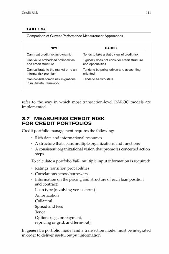
refer to the way in which most transaction-level RAROC models are implemented.

3.7 MEASURING CREDIT RISK FOR CREDIT PORTFOLIOS

Credit portfolio management requires the following:

• Rich data and informational resources• A structure that spans multiple organizations and functions• A consistent organizational vision that promotes concerted action

steps

To calculate a portfolio VaR, multiple input information is required:

• Ratings transition probabilities• Correlations across borrowers• Information on the pricing and structure of each loan position

and contract:Loan type (revolving versus term)AmortizationCollateralSpread and feesTenorOptions (e.g., prepayment,repricing or grid, and term-out)

In general, a portfolio model and a transaction model must be integratedin order to deliver useful output information.

Credit Risk 141

T A B L E 3-2

Comparison of Current Performance Measurement Approaches

NPV RAROC

Can treat credit risk as dynamic Tends to take a static view of credit risk

Can value embedded optionalities Typically does not consider credit structure and credit structure and optionalities

Can calibrate to the market or to an Tends to be policy driven and accounting internal risk premium oriented

Can consider credit risk migrations Tends to be two-statein multistate framework


3.7.1 Economic Capital Allocation

3.7.1.1 Probability Density Function of Credit LossesSophisticated financial organizations use an analytical setup that relates theoverall required economic capital of the institute to its credit activities. The required economic capital is linked to the portfolio’s credit risk with theprobability density function (PDF) of credit losses, a key result from the creditrisk model.10 An important element is the probability that credit losses willexceed a given amount, which is represented by the area under the densityfunction to the right of the given limit (the upper limit covering expectedcredit losses). A portfolio with a higher risk of credit loss is one whose den-sity under the function has a relatively long and fat tail (see Figure 3-6).

The expected credit loss is defined as the total amount of credit lossesthe bank would expect from its credit portfolio over a specific time hori-zon (leftmost vertical line in Figure 3-6). The expected loss is one of thecosts of transacting business that gives rise to credit risk. For marketingand other reasons, financial institutes prefer to express the risk of thecredit portfolio by the unexpected credit loss, i.e., the amount by which theactual losses exceed the expected loss. The unexpected loss is a measure ofthe uncertainty or variability of actual losses versus expected losses. Theestimated economic capital needed to support the institution’s credit port-folio activities is generally referred to as its required economic capital forcredit risk. A cushion of economic capital is required for loss absorption,

142 CHAPTER 3

Allocated economic capital

Expected credit loss

99% confidence level1% loss

Extreme credit losses — tail events

Prob

abili

ty

Covered byadequate pricingand lossprovisions

Covered by loss provisions and/orproprietary capital

Covered by loss provisions and/orproprietary capital quantified usingscenario analysis and controlled withconcentration limits

F I G U R E 3-6

Probability Density Function (PDF) of Credit Losses.


because the actual level of credit losses suffered in any one period couldbe significantly higher than the expected level. The procedure for calcu-lating this amount is similar to the VaR methods used in allocating eco-nomic capital for market risks. The understanding is that economic capitalfor credit risk is determined in such a way that the estimated probabilityof unexpected credit loss exhausting economic capital is less than sometarget insolvency rate.

The capital allocation systems generally assume that it is the role ofreserve funding to cover expected credit losses, while it is the role of eco-nomic capital to cover unexpected credit losses. The required economiccapital represents the additional amount of capital necessary to achievethe target insolvency rate, over and above that needed for coverage of ex-pected losses (the distance between the two lines in Figure 3-6).

3.7.1.2 Measuring Credit LossLoss in a credit portfolio is defined by three variables: the difference be-tween the portfolio’s current value and its future value at the end of a certaintime horizon. Because many functions depend on the time dimension inone way or another, the time horizon is a key input variable for the defini-tion of risk. There are basically two ways of selecting the time horizonover which credit risk is monitored:

• The first approach is the application of a standardized time periodacross all contracts (instruments). Most financial institutionsadopt a one-year time horizon across all asset classes (not onlycredit instruments).

• The second is the liquidation period approach, in which eachcredit contract (instrument) is associated with a unique timeperiod, coinciding with the instrument’s maturity or with thetime needed for liquidation. Some vendor systems allowspecific time periods for asset classes or portfolios (forstructured credit portfolios). The hold-to-maturity approachseems to be applicable if the exposures were intended to be heldto maturity and/or liquid markets for trading these instrumentsare limited.

The factors influencing the fixing of the period are as follows:

• Availability or publication of default information• Availability of borrower information• Internal control rhythms and renewal processes• Capital planning• Account statement preparations; changes to the capital structure

(capital increase or reduction).

Credit Risk 143


3.7.1.3 Default-Mode ParadigmThe default-mode (DM) paradigm states that a credit loss occurs only if aborrower defaults on a repayment obligation within the planning horizon.As long as the default event does not become a fact, no credit loss wouldexist. In the event that the borrower defaults on obligations, the credit lossis calculated as the difference between the bank’s credit exposure (theamount due to the bank at the moment of default) and the present valueof future net recoveries (discounted cash flows from the borrower lessworkout expenses). The current and the future values of the credit are de-fined in the default-mode paradigm based on the underlying two-state(default versus nondefault) notion of the credit loss. The current value istypically calculated as the bank’s credit exposure (e.g., book value). Thefuture value of the loan is uncertain. It would depend on whether the bor-rower defaults during the defined time horizon. In the case of nondefault,the credit’s future value is calculated as the bank’s credit engagement atthe end of the time horizon (adjusted so as to add back any principal pay-ments made over the time horizon).

In the case of a default, the future value of the credit is calculated asthe credit minus loss rate given default (LGD). The higher the recovery ratefollowing default, the lower the LGD. Using a credit risk model, the cur-rent value of the credit instrument is assumed to be known, but the futurevalue is uncertain. Applying a default-mode credit risk model for each in-dividual credit contract (e.g., loan versus commitment versus counter-party risk), the financial institution must define or estimate the jointprobability distribution between all credit contracts with respect to threetypes of random variables:

• The bank’s associated credit exposure• A binary zero/one indicator denoting whether the credit contract

defaults during the defined time horizon• In the event of default, the associated LGD

3.7.1.4 Mark-to-Market ParadigmThe mark-to-market (MTM) paradigm treats all credit contracts under theassumption that a credit loss can arise over time, deteriorating the asset’scredit quality before the end of the planned time horizon. The mark-to-market paradigm treats all credit contracts as instruments of a portfoliobeing marked to market (or, more accurately, marked to model) at the be-ginning and end of the defined time horizon. The credit loss reflects thedifference of the valuation at the beginning and at the end of the time hori-zon. This approach considers changes in the asset’s creditworthiness, re-flecting events that occur before the end of the time horizon. These modelsmust incorporate the probabilities of credit rating migrations (through therating transition matrix), reflecting the changes in creditworthiness.

144 CHAPTER 3


For each credit position in the portfolio, migration paths have to becalculated, using the rating transition matrix and Monte Carlo simulation.For all positions, the simulated migration (including the risk premium as-sociated with the contract’s rating grade at the end of the rating period) isused to mark the position to market (or, more accurately, to model) as ofthe end of the time horizon. For the purpose of estimating the current andfuture values of the credit contracts, two approaches can be used:

• The discounted contractual cash flow (DCCF) approach• The risk-neutral valuation (RNV) approach

3.7.1.5 Discounted Contractual Cash Flow ApproachThe discounted contractual cash flow (DCCF) approach is commonly associ-ated with J. P. Morgan’s CreditMetrics methodology. The current value ofa nondefaulted loan is calculated as the present discounted value of its fu-ture contractual cash flows. For a credit contract with an assigned risk rat-ing (i.e., BBB), the credit spreads used for the calculation of the discountedcash flows of the credit contract equal the market-determined term struc-ture of credit spreads corresponding to similar corporate bonds (maturity,coupon, sinking-fund provision, etc.) with that same rating. The currentvalue is treated as known, because the future value of the credit dependson the (uncertain) end-of-period rating and the market-determined termstructure of credit spreads associated with the specific rating. The futurevalue of the credit is subject to changes in migration (creditworthiness) orin the credit spreads according to the market-determined term structure.In the event of default, the future value of a credit would be given by itsrecovery value, calculated as the credit minus loss rate given default (asimilar approach to that used in the default-mode approach).

The DCCF approach is a practical approach, but it is not completely inline with modern finance theory. For all contracts with the same rating, thesame discount rates are assigned. Thus, for all contracts not defaulted withinthe defined time horizon, the future value does not depend on the expectedloss rate given default, as they are not defaulted. Modern finance theoryholds that the value of an asset (borrower’s asset) depends on the correlationof its return with that of the market. Borrowers in different market segments,exposed to different business cycles and other risk factors, will still be as-signed to the same risk grade according to the DCCF approach.

3.7.1.6 Risk-Neutral Valuation ApproachTo avoid the pitfalls of the discounted contractual cash flow approach,Robert Merton developed a structural approach imposing a model of firmvalue and bankruptcy.11 A company defaults when the value of its under-lying assets falls beneath the level required to serve its debt. The risk-neutral valuation (RNV) approach discounts contingent payments instead

Credit Risk 145


of discounting contractual payments. A credit can be considered as a set ofderivative contracts on the underlying value of the borrower’s assets. If apayment (interest rate, amortization, etc.) is contractually due at date t, thepayment actually received by the lender will be the contractual amountonly if the firm has not defaulted by date t. The lender receives a portion ofthe credit’s face amount equal to the credit minus loss rate given default(an approach similar to that used in the default-mode method) if the bor-rower defaults at date t, and the lender receives nothing at date t if the bor-rower has defaulted prior to date t. The value of the credit equals the sumof the present values of these derivative contracts (each payment obliga-tion at time t is regarded as an option). The difference from the discountrates used for the discounted contractual cash flow approach is that the dis-count rate applied to the contracts’ contingent cash flows is determinedusing a risk-free term structure of interest rates and the risk-neutral pricingmeasure. Similar to the option-adjusted spread approach, the risk-neutralpricing measure can be regarded as an adjustment to the probabilities ofborrower default at each horizon t, which incorporates the market risk pre-mium associated with the borrower’s default risk. The magnitude of theadjustment depends on the expected return and volatility of the bor-rower’s asset value. Returns modeled consistently with the capital assetpricing model (CAPM) can be expressed in terms of the market expectedreturn and the firm’s correlation beta (β) with the market. This approachcombines pricing of the credits with the respective credit losses:

• The expected default frequency and the loss rate given default bythe borrower

• The correlation between the borrower’s risk and the systematic(market) risk

This is consistent with modern finance theory.The interpretation of default is key in understanding the risk-neutral

valuation approach. A credit is considered to be in default once it migratesto a predefined limit. This worst-case scenario is not clearly defined; itvaries according to the institution’s risk appetite and risk capacity, thus af-fecting measures of default, migration, credit loss, and the probabilitydensity function.

3.7.2 Choice of Time Horizon

As mentioned earlier, most institutions use a one-year time horizon tomeasure their credit risk exposures. This has to do more with computa-tional convenience and availability of information rather than with inter-nal process and model optimization. The definition of default used incredit models is not congruent with that applied for legal purposes. Theinstitution may consider a credit to be in default if the credit is classified as

146 CHAPTER 3


falling below an investment-grade rating, if cash flows are past due, if thecredit is placed on a nonaccrual status, if recovery proceedings are initi-ated, and so forth.

The time horizon appears to be an important variable for the assess-ment of capacity of models to meet economic and regulatory needs.

The ability of a default-mode model to assess the effects of poten-tially unfavorable credit events due to the model’s two-state nature (i.e.,default/nondefault) may be particularly sensitive to the defined length ofthe time horizon.

3.7.3 Credit Loss Measurement Definition

3.7.3.1 DM Versus MTM ModelsBoth the default-mode (DM) and mark-to-market (MTM) approaches esti-mate the credit losses from adverse changes in credit quality. The qualityof credit models is primarily influenced by the fit between the model out-put and the model application. The model choice should be made basedon the circumstances of the use and application. An institution that uses aportfolio of liquid credits and exposure to credit spreads (i.e., the hedgetransactions for credit portfolios using credit spreads between differentterm structures) may require a credit loss measurement definition that in-corporates potential shifts in credit spreads and thus opt for the (morecomplicated) MTM model with the multistate nature.

3.7.3.2 DCCF Versus RNV ApproachesIn practice, the difference between the approaches is smaller than in theory,because the credit value is priced as a discounted present value of its futurecash flows in both approaches. The dichotomy is sharper in theory becausethe discount factors are calculated differently. The discounted contractualcash flow (DCCF) approach assumes a nonparametric approach to esti-mating these discount factors. The public debt issuers (issues) are groupedinto rating categories, and the credit spreads on the issuers are then aver-aged within each rating “bucket.” On the other hand, the risk-neutral val-uation (RNV) approach is more complex. In a structural process, eachcredit is simultaneously modeled in an individual framework. This meansthat the modeling of the market risk premium for each credit in the RNVmodel is typically referenced to credit spreads from the debt market.

The empirical evidence of the econometric theory shows that highlystructural estimators make efficient use of available data but are vulnera-ble to model misspecification. Nonparametric estimators make minimaluse of modeling assumptions but underperform where data integrity is aproblem. The two approaches will, in general, assign different creditlosses to any given loan. Under normal market conditions (liquidity andinformation efficiency) and the stable assumptions of the RNV model,

Credit Risk 147


both approaches should deliver reasonable output for a well-diversifiedcredit portfolio.

The probability that a particular credit contract will default during thetime horizon is a critical input. The bank’s credit staff has to assign internalcredit risk ratings for all credit contracts. This is done for most corporatecustomers. The trend is that all customers, corporate or retail, are assignedrisk ratings in order to obtain the overall risk profile of the credit portfolio,including the correlations between the different segments of the portfolio asthey are exposed to different business cycles, macroeconomic factors, etc.

There are basically three approaches (which can be combined) for as-signing a credit rating to a customer or the contract:

• The traditional approach, based on financial, accounting, andother characteristics of the customer. This approach is verysubjective and is based on the reliability and availability ofspecific information.

• Credit-scoring models supplied by commercial vendors, whichalso deliver a database that reflects the best-practice standards inthe market.

• Credit-scoring models developed internally, which reflect thestructure and the processes of the credit department.

External ratings are frequently combined with internal rating cate-gories, which allows combination of the internal credit authorizationprocess and external rating data. The expected default frequency (EDF) canbe interpreted as a credit’s probability of migrating from its current inter-nal rating grade to default within the credit model’s time horizon. The like-lihood of such a migration from its current risk rating category to anothercategory is defined in the transition matrix, as illustrated in Table 3-3.

Given the contract’s actual rating (defined by each row), the proba-bility to migrate to another category (defined by the columns) is definedwithin the intersecting cell of the transition matrix. Thus, in Table 3-3, thelikelihood of a credit contract rated A migrating to BBB within one yearwould be 7.4 percent. The likelihood of a credit contract rated CCC mi-grating to default within one year would be 18.6 percent.

3.7.3.3 Unconditional Versus Conditional ModelsIn a broad sense, all models are conditional, as they process input infor-mation on the credit quality of the borrower and the credit contracts. In anarrower sense, it is possible to distinguish between unconditional andconditional models. The unconditional models process information lim-ited to the borrower and the credit contracts. The transition matrix and thecorrelations are modeled to capture the long-run values of these parame-ters. But such long-run averages may misrepresent the short-term condi-tion, as correlations and default frequency tend to vary systematically

148 CHAPTER 3


with the course of the business cycle. The conditional models process in-formation on the borrower and the credit contracts and, in addition, arelinked to macroeconomic information such as gross domestic product,current levels and trends in domestic and international employment, in-flation rates, indicators specific for particular sectors, etc.

CreditMetrics and CreditRisk are examples of unconditional risk mod-els. They estimate the expected default frequency and correlations betweenhistorical default data and borrower- or contract-specific information, suchas the rating. These models are based on data collected and estimated overmany credit cycles to reflect the averages of these parameters. They shouldpredict reasonable credit loss probabilities based on the transition matrix, ifthe credit portfolio is composed of similar credit contracts. This type ofmodel has drawbacks; if the borrowers are upgraded or downgraded overtime, their expected default rates will be revised downward or upward.Such a portfolio will not have a similar standard deviation over time andwill be more complex to manage relative to given risk levels. The uncondi-tional models are not able to incorporate macroeconomic parameters suchas business cycle effects. The tendency for rating improvement or deteriora-tion is positive during cyclical upturns or downturns, respectively.

The drawbacks of the unconditional models are avoided with the con-ditional models. Examples of conditional credit risk models include McKin-sey and Company’s CreditPortfolioView12 and KMV’s PortfolioManager.

Credit Risk 149

T A B L E 3-3

Sample Credit Rating Transition Matrix: Probability of Migrating to Another Rating Within 1 Year

Rating at Year End, %Initial Rating AAA AA A BBB BB B CCC Default

AAA 87.74 10.93 0.45 0.63 0.12 0.10 0.02 0.02

AA 0.84 88.23 7.47 2.16 1.11 0.13 0.05 0.02

A 0.27 1.59 89.05 7.40 1.48 0.13 0.06 0.03

BBB 1.84 1.89 5.00 84.21 6.51 0.32 0.16 0.07

BB 0.08 2.91 3.29 5.53 74.68 8.05 4.14 1.32

B 0.21 0.36 9.25 8.29 2.31 63.89 10.13 5.58

CCC 0.06 0.25 1.85 2.06 12.34 24.86 39.97 18.60

SOURCE: Greg M. Gupton, Christopher C. Finger, and Mickey Bhatia, CreditMetrics Technical Document, New York: MorganGuaranty Trust Co., April 1997, 76. Copyright © 1997 by J. P. Morgan & Co., Inc., all rights reserved. Reproduced withpermission of RiskMetrics Group, Inc.


Within its conceptual modeling, the transition matrices of CreditPortfo-lioView are related to the state of the economy, as the matrices of the covari-ance matrix are modified to give an increased likelihood of an upgrade (anddecreased likelihood of a downgrade) during an upswing (or downswing)in a credit cycle. KMV’s PortfolioManager links the process of estimatingthe asset values, rates of return, and volatility to current equity prices,which are information-efficient and incorporate all information available inthe market. This approach is comparable to the arbitrage price theory (APT)and the multifactor models. Empirical research has generated empirical ev-idence. The drawbacks of these models are timing and parameterization.They might underestimate losses as the credit cycle enters a downturn andoverestimate losses as the cycle bottoms out.

3.7.4 Risk Aggregation

Within most credit risk approaches, broadly similar conceptual approachesare implemented, modeling individual-level credit risk exposures for dif-ferent type of positions. Most banks measure credit risk at the individualasset level for capital market and corporate instruments (bottom-up ap-proach), while aggregate data is used for quantifying risk for different typesof positions (top-down approach), including product lines such as consumer,credit card, or mortgage portfolios.

• Bottom-up approaches attempt to measure credit risk at theindividual level of each facility based on an explicit evaluation ofthe creditworthiness of the portfolio’s constituent debtors. Eachspecific position in the portfolio is linked with an individual riskrating, typically used as a proxy for the EDF or the probability ofrating migration.13 The data is then aggregated to the portfoliolevel, taking into account diversification effects based on thecorrelation matrix.

• Top-down approaches are used to cope with the sheer number ofexposures. Typically, for retail positions, a top-down empiricalapproach is applied. The information for individual positions isallocated to specific factors and aggregated into buckets, such ascredit scores, age, geographical location, collateralized exposures,and so forth. The credit risk is quantified at the level of thesebuckets. Facilities within each bucket are treated as statisticallyidentical. In the process of estimating the distribution of creditlosses, the model builder would attempt to model both theaggregate default rate and the LGD rate using historical time-seriesdata for that risk segment (bucket) taken as a whole, rather than byarriving at this average through a joint consideration of default andmigration risk factors for each specific facility in the pool.

150 CHAPTER 3


The literature on credit risk models tends to make a distinction be-tween these two approaches, whereas in practice the differences are lessclear-cut. The differences in the implementation arise primarily in the waysthe underlying parameters are estimated using the available data. The dis-tinction between top-down and bottom-up approaches is not always pre-cise. The key consideration is the degree to which a financial institution candistinguish meaningfully between borrower classes (buckets). Frequently,so-called bottom-up models rely on aggregate data to estimate individualborrower parameters. A practical example is the mapping of individual bor-rower ratings (a bottom-up approach) to a transition matrix calculated frompooled data, which is derived from published ratings by rating agencies orfrom internal statistics (an average of aggregate top-down data). The accu-racy of aggregate data and the compatibility to the financial institution’s ac-tual credit portfolio influences the use of aggregate data and potentiallydistorts idiosyncratic loan-specific effects to which the financial institutionis exposed.

3.8 DEVELOPMENT OF NEW APPROACHES TO CREDIT RISK MANAGEMENT

3.8.1 Background

Over the past few years, a revolution has been brewing in the way creditrisk is both measured and managed. In contrast to the accounting-driven,relatively dull, and routine history of credit risk, new technologies andmethodologies have emerged among a new generation of financial engi-neering professionals who are applying their engineering skills andanalysis to this risk topic.

Why is this development happening now? The eight most obviousreasons for this sudden surge in interest are as follows:

• Maturing market risk area. Given the maturity of market riskmodels, the experience gained over the past decades, based ontheoretical and academic research and practical experience whichhas relativized and improved the relevance of market riskmodeling, the market risk area has evolved in a way that freesresources and welcomes new challenges, such as credit andoperational risk.

• Disintermediation of borrowers. As capital markets have expandedand become accessible to small- and middle-market firms,borrowers left behind to raise funds from banks and othertraditional financial institutions are increasingly likely to besmaller and have weaker credit ratings. Capital market growthhas produced a “winner’s curse” effect on the credit portfoliostructure of traditional financial institutions.

Credit Risk 151


• Competitive margin structure. Almost paradoxically, despite adecline in the average quality of loans (due to disintermediation),the respective margin spreads, especially in wholesale loanmarkets, have become very thin—that is, the risk–premiumtrade-off from lending has gotten worse. A number of reasons canbe cited, but an important factor is the enhanced competition forlower-quality borrowers, such as from finance companies, muchof whose lending activity is concentrated at the higher-risk,lower-quality end of the market.

• Structural change in bankruptcies. Although the most recentrecessions hit at different times in different countries, mostbankruptcy statistics showed a significant increase inbankruptcies, compared to the prior economic downsides. To theextent that there has been a permanent or structural increase inbankruptcies worldwide—possibly due to the increase in globalcompetition and sectoral changes, such as the technologysector—accurate credit risk analysis becomes even moreimportant today than in the past.

• Diminishing and volatile values of collaterals. Concurrent with theongoing Asian crisis, banking crises in well-developed countrieshave shown that real estate values and precise asset values arevery hard to predict and to realize through liquidation. Theweaker the rating and the more uncertain collateral values are,the more risky lending is likely to be.

• Exposures from off-balance-sheet derivatives. The growth of creditexposure and counterparty risk, based on the phenomenalgrowth of the derivative markets, has extended the need forcredit analysis beyond the loan book. In many of the largestbanks, the notional (not market) value of the off-balance-sheetexposure to instruments such as over-the-counter (OTC) swapsand forwards exceeds more than 10 times the size of the loanportfolios. The growth in credit risk off the balance sheet was oneof the reasons for the introduction of risk-based capitalrequirements in 1993.14

• Capital requirements. Under the BIS system, banks have to hold acapital requirement based on the marked-to-market current valueof each OTC derivatives contract (so-called current exposure)plus an add-on for potential future exposure.

• Technological advances. Computer infrastructure developmentsand related advances in information technology—such as thedevelopment of historic information databases—have givenbanks and financial organizations the opportunity to test high-powered modeling techniques. In the case of credit risk

152 CHAPTER 3


management, besides being able to analyze loan loss and valuedistribution functions and especially the tails distributions,the infrastructure enables the active management of loanportfolios, based on modern portfolio theory (MPT) modelsand techniques.15

3.8.2 BIS Risk-Based Capital Requirement Framework

Despite the importance of the reasons previously discussed, probably thegreatest incentive and key impetus to the development of enhanced creditrisk models has been dissatisfaction with the BIS and local regulators’ im-position of capital requirements on loans. The current BIS regime has beendescribed as a “one size fits all” policy; virtually all loans to private-sectorcounterparties are subjected to the same 8 percent capital ratio (or capitalreserve requirement), not taking into account the different impacts of thesize of the loan; the maturity of the loan; or, most important, the creditquality (rating) of the borrowing counterparty. Under current capital re-quirement terms, loans to a firm near bankruptcy are treated in the samefashion as loans to a AAA borrower or the government. Further, the cur-rent capital requirement is additive across all loans; there is no allowancefor lower capital requirements because of a greater degree of diversifica-tion in the loan portfolio.

In 1997, the European Community was the first to give certain largebanks the discretion to calculate capital requirements for their tradingbooks—or market risk exposures—using internal models rather than the al-ternative regulatory (standardized) model. Internal models are subject tocertain constraints imposed by regulators and are subjected to backtestingverification.16 They potentially allow the following revisions:

• VaR of each tradable instrument to be more accurately measured(e.g., based on its price volatility, maturity, etc.)

• Correlations among assets (diversification effect) to be taken intoaccount

In the context of market risk, VaR is defined as the predicted worst-case loss at a specific confidence level (e.g., 95 percent) over a certain pe-riod of time (e.g., 10 days). For example, under the BIS market riskregulations, when banks calculate their VaR-based capital requirementsusing their internal models, they are required to measure the worst-caseday as the worst day that happens once every 100 business days. The cur-rent regulative framework is additive and does not consider diversifica-tion in the loan portfolio to allow lower capital requirements.

The critical questions for bankers and regulators developing a newframework are the following:

Credit Risk 153


• Can an internal-model approach be used to measure the VaR orcapital exposure of (nontradable) loans?

• Do internal models provide sufficient flexibility and accuracy tosupport the standardized 8 percent risk-based capital ratio thatimposes the same capital requirement on virtually all private-sector loans?

Internal models require additional enhancements before they can re-place the 8 percent rule, especially because of the nontradability of sometypes of loans compared to marketable instruments, and the lack of deep his-toric databases on loan defaults. However, the new internal models offeradded value to financial organizations, regulators, and risk managers. Specif-ically, internal model approaches potentially offer better insight on how tovalue and manage outstanding loans and credit risk–exposed instrumentssuch as bonds (corporate and emerging market), as well as better methods forestimating default risk probabilities regarding borrowers and derivativecounterparties. Moreover, internal models have the following advantages:

• In many cases they allow a better estimation of the credit risk ofportfolios of loans and credit risk–sensitive instruments.

• They enhance the pricing of new loans, in the context of a bank’sRAROC, and of relatively new instruments in the creditderivatives markets (such as credit options, credit swaps, andcredit forwards). The models provide an alternative opportunityto measure the optimal or economic amount of capital a bankshould hold as part of its capital structure.

Before looking at some of these models and new approaches to creditrisk measurement, a brief analysis of the more traditional approaches willheighten the contrast between the new and traditional approaches tocredit risk measurement.

3.8.3 Traditional Credit Risk Measurement Approaches

3.8.3.1 BackgroundIt is hard to draw a clear line between traditional and new approaches, asmany of the superior concepts of the traditional models are used in thenew models. For the purposes of this historical review, the traditionalcredit models are segregated into three types: expert systems, rating sys-tems, and credit-scoring systems.17

3.8.3.2 Expert SystemsIn an expert system, the credit decision is made by the local or branchcredit officer. Implicitly, this person’s expertise, skill set, subjective judg-

154 CHAPTER 3


ment, and weighting of certain key factors are the most important deter-minants in the decision to grant credit. The potential factors and expertsystems a credit officer could look at are infinite. However, one of the mostcommon expert systems, the “five Cs” of credit, will yield sufficient un-derstanding. The expert analyzes these five key factors, subjectivelyweights them, and reaches a credit decision:

• Capital structure. The equity-to-debt ratio (leverage) is viewed as a good predictor of bankruptcy probability. High leveragesuggests greater probability of bankruptcy than low leverage, as alow level of equity reduces the ability of the business to survivelosses of income.

• Capacity. The ability to repay debts reflects the volatility of theborrower’s earnings. If repayments on debt contracts proves to bea constant stream over time, but earnings are volatile (and thushave a high standard deviation), the probability is high that thefirm’s capacity to repay debt claims is at risk.

• Collateral. In the event of a default, a lender has a claim on thecollateral pledged by the borrower. The greater the proportion ofthis claim and the greater the market value of the underlyingcollateral, the lower the remaining exposure risk of the loan in thecase of a default.

• Cycle/economic conditions. An important factor in determiningcredit risk exposure is the state of the business cycle, especiallyfor cycle-dependent industries. For example, the infrastructuresectors (such as the metal industries, construction, etc.) tend to bemore cycle dependent than nondurable goods sectors, such asfood, retail, and services. Similarly, industries that have exposureto international competitive conditions tend to be cycle sensitive.Taylor, in an analysis of Dun and Bradstreet bankruptcy data byindustry (both means and standard deviations), found some quitedramatic differences in U.S. industry failure rates during thebusiness cycle.18

• Character. This is a measure of the firm’s reputation, itswillingness to repay, and its credit history. In particular, it hasbeen established empirically that the age factor of an organizationis a good proxy for its repayment reputation.

Another factor, not covered by the five Cs, is the interest rate. It is well known from economic theory that the relationship between the interest-rate level and the expected return on a loan (loss probability) ishighly nonlinear.19 At low interest-rate levels, the expected return could in-crease if rates are raised. However, at high interest-rate levels, an increasein rates may lower the return on a loan, as the probability of loss increases.

Credit Risk 155


This negative relationship between high loan rates and expected loan re-turns is due to two effects: (1) adverse selection and (2) risk shifting. Whenloan rates rise beyond some point, good borrowers drop out of the loanmarket, preferring to self-finance their investment projects or to seek equity capital funding (adverse selection). The remaining borrowers, whohave limited liability and limited equity at stake—and thus lower rat-ings—have the incentive to shift into riskier projects (risk shifting). In up-side economies and supporting conditions, they will be able to repay theirdebts to the bank. If economic conditions weaken, they will have limiteddownside loss from a borrower’s perspective.

Although many financial institutions still use expert systems as partof their credit decision process, these systems face two main problems re-garding the decision process:

• Consistency. What are the important common factors to analyzeacross different types of groups of borrowers?

• Subjectivity. What are the optimal weights to apply to the factorschosen?

In principle, the subjective weights applied to the five Cs derived by an ex-pert can vary from borrower to borrower. This makes comparability ofrankings and decisions across the loan portfolio very difficult for an indi-vidual attempting to monitor a personal decision and for other experts ingeneral. As a result, quite different processes and standards can be appliedwithin a financial organization to similar types of borrowers. It can be ar-gued that the supervising committees or multilayered signature authoritiesare key mechanisms in avoiding consistency problems and subjectivity, butit is unclear how effectively they impose common standards in practice.20

3.8.3.3 Rating SystemsOne of the oldest rating systems for loans was developed by the U.S. Of-fice of the Comptroller of the Currency (OCC). The system has been usedin the United States by regulators and bankers to assess the adequacy oftheir loan loss reserves. The OCC rating system allocates an existing loaninto five rating buckets: four low-quality ratings and one high-quality rat-ing. In Table 3-4, the required loss reserve appears next to each category.

Over the years, the financial institutions have extended and en-hanced the OCC-based rating system by developing internal rating sys-tems that more finely subdivide the pass/performing rating category.

The OCC pass grade is divided into six different categories (ratings1 to 6). Ratings 7 to 10 correspond to the OCC’s four low-quality loan rat-ings. These loan-rating systems do not exactly correspond with the bond-rating systems, especially at the lower-quality end of the spectrum (seeSection 2.7.2.4 for a further discussion of bond-rating systems). One rea-son is the different focus of the approaches: loan-rating systems are sup-

156 CHAPTER 3


posed to rate an individual loan (including its covenants and collateralbacking). Bond-rating systems are more oriented toward rating the over-all borrower. This gap of one-to-one mapping between bond and loan rat-ing methodologies raises a flag as to the merits of those newer approachesthat rely on bond data (spreads, transition matrices, etc.) to value andprice loans individually and in a portfolio context.

Given this trend toward finer internal ratings of loans, compared tothe OCC’s regulatory model, the 1998 Federal Reserve System Task ForceReport21 and Mingo22 give some tentative support for using an internalmodel ratings-based approach as an alternative to the OCC model, to cal-culate capital reserves against unexpected losses, and loan loss reservesagainst expected loan losses. For example, using the outstanding dollarvalue of loans in each internal rating class (1 to 10), a bank might calculateits capital requirement against unexpected loan losses as follows:

total class 1 loans ⋅ 0.2%+

Capital requirement = Σ� � � (3.1)+

total class 10 loans ⋅ 100%

The 0.2 percent for rating class 1 is just suggestive of unexpected lossrates and should be based on historic loss probabilities of a loan in class 1moving to class 10 (loss) over the next year.23 However, an important prob-

Credit Risk 157

T A B L E 3-4

Example for Loss Reserves Based on Rating System

Rating Bucket Loss Reserves, %

Low-quality ratings

Other assets especially mentioned (OAEM) 0

Substandard assets 20

Doubtful assets 50

Loss assets 100

High-quality rating

Pass/performing 0

NOTE: From a technical perspective, the 0 percent loss reserves for OAEM and pass loans are lower bounds. In practice,the reserve rates on these categories are determined by the bank in consultation with examiners and auditors, dependingon some type of historical analysis of charge-off rates for the bank.

SOURCE: U.S. Office of the Comptroller of the Currency, EC-159 (rev.), December 10, 1979, www.occ.treas.gov/ftp/release.


lem remains, similar to the current 8 percent risk-based capital ratio of theBIS approach—the diversification in the loan portfolio is not considered.The credit risks of each rating class are simply added up to calculate a totalcapital requirement.

3.8.3.4 Credit-Scoring SystemsCredit-scoring approaches can be found in virtually all types of creditanalysis. The basic concept is generally the same: certain key factors arepreidentified. They determine the loss probability of default and the recov-ery rate (as opposed to repayment), and they are combined or weightedinto a quantitative score schema. The score can be literally interpreted as aloss probability of default. In other scoring systems, the score can be re-garded as a classification system: it allocates a potential or existing bor-rower into either a good group (higher rating) or a bad group (lowerrating), based on a score and a cutoff point. Full reviews of the traditionalapproach to credit scoring, and the various methodologies, can be found inCaouette, Altman, and Narayanan24 and in Saunders.25 See Altman andNarayanan for a good review of the worldwide application of credit-scoring models.26 One simple example of this new credit risk model typeshould cover the key issues supposedly addressed by many of these newermodels. The Altman Z-score model is a classification model for corporateborrowers and can also be used to get a default probability prediction.27

Based on a matched sample by year, size, and sectors of defaulted and sol-vent firms, and applying the linear discriminant analysis, the best-fittingscoring model for commercial loans results in the following equation:

Z = 1.2 ⋅ X1 + 1.4 ⋅ X2 + 3.3 ⋅ X3 + 0.6 ⋅ X4 + 1.0 ⋅ X5 (3.2)

where X1 = working capital/total assets ratioX2 = retained earnings/total assets ratioX3 = earnings before interest and taxes/total assets ratioX4 = market value of equity/book value of total liabilities ratioX5 = sales/total assets ratio

If a corporate borrower’s accounting ratios Xi, weighted by the esti-mated coefficients in the Z function, result in a Z score below a criticalvalue (in Altman’s initial study, 1.81), the borrower would be classified as“insufficient” and the loan would be refused.

A number of issues need to be discussed here. First, the model is lin-ear, whereas the path to bankruptcy can be assumed to be highly nonlin-ear, and the relationship between the Xi values itself is likely to benonlinear. A second issue is that, with the exception of the market value ofequity term in the leverage ratio, the model is essentially based on ac-counting ratios. In most countries, standards require accounting data only

158 CHAPTER 3


at discrete intervals (e.g., quarterly) and are generally based on historic- orbook-value accounting principles. It is also questionable whether suchmodels can capture the momentum of a firm whose condition is rapidlydeteriorating (e.g., as in the Russia crisis of October 1998). As the worldbecomes more complex and competitive, and the decision flow becomesfaster, the predictability of simple Z-score models may worsen. Brazil of-fers a good example. When fitted in the mid-1970s, the Z-score model dida quite good job of predicting default even two or three years prior tobankruptcy.28 However, more recently, even with low inflation and greatereconomic stability, this type of model has performed less well as theBrazilian economy has become more open.29

The recent application of nonlinear methods (such as neural net-works) to credit risk analysis shows potential to improve on the provencredit-scoring models. Rather than assuming there is only a linear and di-rect effect from the Xi variables on the Z credit score (or, in the language ofneural networks, from the input layer to the output layer), neural net-works allow for additional explanatory power via complex correlations orinteractions among the Xi variables (many of which are nonlinear). For ex-ample, the five variables in the Altman Z-score model can be described bysome nonlinearly transformed sum of X1 and X2 as a further explanatoryvariable.30 In neural network terminology, the complex correlationsamong the Xi variables form a “hidden layer” which, when exploited (i.e.,included in the model), can improve the fit and reduce type 1 and type 2errors. (A type 1 error consists of misjudging a bad loan as good; a type 2error consists of misjudging a good loan as bad.)

Yet, neural networks pose many problems for financial economists.How many additional hidden correlations should be included? In thelanguage of neural networks, when should training stop? It is entirelypossible that a large neural network, including large N nonlinear trans-formations of sums of the Xi variables, can reduce type 1 and type 2 errorsof a historic loan database close to zero. However, as is well known, thiscreates the problem of overfitting—a model that well explains in-sampledata may perform quite poorly in predicting out-of-sample data. Moregenerally, the issue is when does one stop adding variables—when the re-maining forecasting error is reduced to 10 percent, 5 percent, or less? Re-ality might prove that what is thought to be a global minimum forecasterror may turn out to be just a local minimum. In general, the issue of eco-nomic meaning is probably the most troubling aspect of financial inter-pretation and use. For example, what is the economic meaning of anexponentially transformed sum of the GARCH-adjusted sales to total as-sets and the credit-spread-adjusted discount factor ratio? The ad hoc eco-nomic nature of these models and their tenuous links to existing financialtheory separate them from some of the newer models that are discussedin the following chapters.

Credit Risk 159


3.8.4 Option Theory, Credit Risk, and the KMV Model

3.8.4.1 BackgroundThe idea of applying option pricing theory to the valuation of risky loansand bonds has been in the literature at least as far back as Merton.31 In re-cent years, Merton’s approach has been extended in many directions. KMVCorporation’s CreditMonitor model, a default prediction model that pro-duces (and updates) default predictions for all major companies and bankswhose equity is publicly traded, is one well-known and widely applied op-tion theory–based loan valuation model.32 This section explains the link be-tween loans and options, then investigates how this link can be used toderive a default prediction model. (Option theory is discussed in more de-tail in Section 2.4.5.)

3.8.4.2 Loans as OptionsFigure 3-7 demonstrates the link between loans and optionality. Assumethat this represents a one-year loan and the amount OB is borrowed on adiscount basis. Technically, option formulas model loans as zero-couponbonds with fixed maturities. Over the year, the borrowing firm will investthe funds in various investments or assets. Assuming that at the end of theyear the market value of the borrowing firm’s assets is OA2 , the borrowerhas an incentive to repay the loan (OB) and keep the residual as profit or re-turn on investment (OA2 − OB). Indeed, for any value of the firm’s assets ex-ceeding OB, the owners of the firm will have an incentive to repay the loan.However, if the market value of the firm’s assets is less than OB (e.g., OA1 inFigure 3-7), the owners have an incentive (or option) to default and to turnover the remaining assets of the firm to the lender (the bank).

160 CHAPTER 3

0 A 21 B AAssets

Payo

ff $

F I G U R E 3-7

Link Between Loans and Optionality.


For market values of assets exceeding OB, the bank will earn a fixed up-side return on the loan; essentially, interest and principal will be repaid in full.For asset values less than OB, the bank suffers increasingly large losses. In theextreme case, the bank’s payoff is zero: principal and interest are a total loss.33

The loan payoff function shown in Figure 3-7—a fixed payoff on theupside and a long-tailed downside risk—looks familiar to an option theo-rist. Comparing this profile with the payoff profile of a short put option ona stock (shown in Figure 3-8) makes the correspondence more obvious. Ifthe price of the stock S exceeds the strike price K, the writer of the optionwill keep the put premium received. If the price of the stock falls below K,the writer will lose successively larger amounts.

Merton noted this formal payoff equivalence; that is, if a bank grantsa loan, its payoff is isomorphic to short a put option on the assets of the bor-rowing firm.34 Moreover, just five variables enter the classic Black-Scholes-Merton model of a put option valuation for stocks (equity capital); thevalue of the default option (or, more generally, the value of a risky loan)will also depend on and reflect on the value of five similar variables.

In general form:

Value of a put option on a stock = f(S,K,r,T,σS) (3.3)

Value of a default option on a risky loan = f(E�,B,r,T,σ�E) (3.4)

where S, K, E, and B are as previously defined (a bar above a variable de-notes that it is not directly observable); r is the short-term interest rate; Eand σE are, respectively, the volatilities of the firm’s equity value and themarket value of its assets; and r is the maturity of the put option or, in thecase of loans, the time horizon (default horizon) for the loan.

Credit Risk 161

K

Stock price S

Payo

ff $

+

-

0

F I G U R E 3-8

Payoff Profile of a Written Put Option on a Stock.


In general, for options on stocks, all five variables on the right-handside of Equation (3.3) are directly observable; however, this is true for onlythree variables on the right-hand side of Equation (3.4). The market valueof a firm’s assets E and the volatility of the market value of a firm’s assetsσE are not directly observable. If E and σE could be directly measured, thevalue of a risky loan, the value of the default option, and the equilibriumspread on a risky loan over the risk-free rate could all be calculated.35

Some analysts have substituted the observed market value of riskydebt on the left-hand side of Equation (3.4) (or, where appropriate, the ob-served interest spread between a firm’s risky bonds and a matched risk-free Treasury rate) and have assumed that the book value of assets equalsthe market value of assets. This allows the implied volatility of assets σE tobe backed out from Equation (3.4).36 However, without additional as-sumptions, it is impossible to input two unobservable values (E and σE),based solely on one equation [Equation (3.4)]. Moreover, the market valueof risky corporate debt is hard to get for all but a few firms.37 Corporatebond price information is generally not easily available to the public, andquoted bond prices are often artificial matrix prices.37

3.8.4.3 KMV CreditMonitor ModelThe innovation of the KMV CreditMonitor model is that it looks at thebank’s lending problem from the viewpoint of the borrowing firm’s eq-uity holders and considers the loan repayment incentive problem (see bib-liography). To solve the two unknown variables, E and σE, the system usesthe following relationships:

• The structural relationship between the market value of a firm’sequity and the market value of its assets.

• The relationship between the volatility of a firm’s assets and thevolatility of a firm’s equity. After values of these variables arederived, an expected default frequency (EDF) measure for theborrower can be calculated.

Figure 3-9 shows the loan repayment issue from the side of the bor-rower (the equity owner of the borrowing firm). Suppose the firm borrowsOB and the end-of-period market value of the firm’s assets is OA2 (whereOA2 > OB). The firm will then repay the loan, and the equity owners willkeep the residual value of the firm’s assets (OA2 − OB). The larger the mar-ket value of the firm’s assets at the end of the loan period, the greater theresidual value of the firm’s assets to the equity holders (borrowers). How-ever, if the firm’s assets fall below OB (e.g., are equal to OA1), the borrowersof the firm will not be able to repay the loan.39 They will be economically in-solvent, will declare bankruptcy, and will turn the firm’s assets over to thebank. Note that the downside risk to the equity owners is truncated no mat-ter how low asset values are, compared to the amount borrowed. Specifi-

162 CHAPTER 3


cally, “limited liability” protects the equity owners against losing more thanOL (the owners’ original stake in the firm). As shown in Figure 3-9, the pay-off to the equity holder of a leveraged firm has a limited downside and along-tailed upside. Being familiar with options, we recognize the similaritybetween the payoff function of an equity owner in a leveraged firm andbuying a call option on a stock. Thus, we can view the market-value posi-tion of equity holders in a borrowing firm E as isomorphic to holding a calloption on the assets of the firm A.

In general terms; equity can be valued as:

E = h(A�,σ�A,r,B,T) (3.5)

In Equation (3.5), the observed market value of a borrowing firm’sequity (price of shares × number of shares) depends on the same five vari-ables as in Equation (3.4), as per the Black-Scholes-Merton model for valu-ing a call option (on the assets of a firm). However, a problem still remains:how to solve two unknowns (A and σA) from one equation (where E, r, B,and T are all observable).

KMV and others in the literature have resolved this problem by not-ing that a second relationship can be exploited: the theoretical relationshipbetween the observable volatility of a firm’s equity value σE� and the un-observable volatility of a firm’s asset value σA. In general terms:

σ�E = g(σA) (3.6)

Credit Risk 163

Val

ue o

f eq

uity

E, $

-L

Value of assets A

Amount OA2

Amount OB

Loss

0

BA1 A2

F I G U R E 3-9

Call Option to Replicate the Equity of a Firm.


With two equations and two unknowns, Equations (3.5) and (3.6) canbe used to derive a solution for A and σA by successive iteration. Explicitfunctional forms for the option-pricing model (OPM) in Equation (3.5) andfor the stock price–asset volatility linkage in Equation (3.6) have to be spec-ified.40 KMV uses an option-pricing Black-Scholes-Merton-type model thatallows for dividends. B, the default exercise point, is taken as the value ofall short-term liabilities (one year and under), plus half the book value ofoutstanding long-term debt. While the KMV model uses a framework sim-ilar to that of Black-Scholes-Merton, the actual model implemented, whichKMV calls the Vasicek-Kealhofer model, makes a number of changes in orderto produce usable results. These modifications include defining five classesof liabilities, reflecting cash payouts such as dividends, handling convert-ible debt, assuming the default point is an absorbing barrier, and relying onan empirical distribution to convert distance to default into a default prob-ability. The precise strike price or default boundary has varied under dif-ferent generations of the model. There is a question as to whether netshort-term liabilities should be used instead of total short-term liabilities.41

The maturity variable t can also be altered according to the default horizonof the analyst; it is most commonly set equal to one year. A slightly differ-ent OPM was used by Ronn and Verma to solve a very similar problem, es-timating the default risk of U.S. banks.42

After they have been calculated, the A and σA values can be em-ployed, along with assumptions about the values of B and T, to generate atheoretically based EDF score for any given borrower.

The idea is shown in Figure 3-10. Suppose that the values backed outof Equations (3.5) and (3.6) for any given borrower are, respectively, A =

164 CHAPTER 3

t = 0

A = $100 M

t = 1

Default region

Time t

B = $80 M

Standarddeviation Aσ+

Aσ-Standarddeviation

F I G U R E 3-10

Theoretical EDF and Default Loss Region


$100 million and σA = $10 million, where σA is the annual standard devia-tion of the asset value. The value of B is $80 million. In practice, the usercan set the default boundary or exercise price B equal to any proportion oftotal debt outstanding that is of interest. Suppose we want to calculate theEDF for a one-year horizon. Given the values of A, σA, B, and r, and with requal to one year, what is the theoretical probability of a borrowing firm’sfailure at the one-year horizon? As can be seen in Figure 3-10, the EDF isthe cross-hatched area of the distribution of asset values below B. Thisarea represents the probability that the current value of the firm’s assets,$100 million, will drop below $80 million at the one-year time horizon.

If it is assumed that future asset values are normally distributedaround the firm’s current asset value, we can measure the t = 0 (or today’s)distance from default at the one-year horizon as follows:

Distance from default = �A

σ−

A

B� =�

$100$M10

−M$80 M�

= 2 standard deviations (3.7)

For the firm to enter the default region (the shaded area), asset valueswould have to drop by $20 million, or 2 standard deviations, during thenext year. If asset values are normally distributed, we know that there is a95 percent probability that asset values will vary between plus and minus2σ from their mean value. Thus, there is a 2.5 percent probability that assetvalues will increase by more than 2σ over the next year, and a 2.5 percentprobability that they will fall by more than 2σ. In other words, there is anEDF of 2.5 percent. We have shown no growth in expected or mean assetvalues over the one-year period in Figure 3-10, but this can easily be in-corporated. For example, if we project that the value of the firm’s assetswill grow 10 percent over the next year, then the relevant EDF would belower because asset values would have to drop by 3σ, which is below thefirm’s expected asset growth path, for the firm to default at year-end. Thedistance from default is:43

�A(1 +

σg

A

) − B� =�

$110$M10

−M$80 M� = 3 standard deviations (3.8)

The normal distribution assumption of asset values around somemean level is critical in calculating joint default transition probabilities inJ. P. Morgan’s CreditMetrics (see Section 3.8.5.3), yet there is an importantissue as to whether it is theoretically or empirically reasonable to makethis assumption. With this in mind, rather than producing theoreticalEDFs, the KMV approach generates an empirical EDF along the follow-ing lines. Suppose that we have a large historic database of firm defaults

Credit Risk 165


and no defaults (repayments), and we calculate that the firm we are ana-lyzing has a theoretical distance from default of 2σ. We then ask the em-pirical questions:

• What percentage of the borrowers in the database actuallydefaulted within the one-year time horizon when their assetvalues placed them a distance of 2σ away from default at thebeginning of the year?

• What is the percentage of the total population of borrowers thatwere 2σ away from default at the beginning of the year?

This produces an empirical EDF:

Empirical EDF =

Number of borrowers that defaulted within a year with asset values of 2σfrom B at the beginning of the year

Total population of borrowers with asset values of 2σ from B at the beginning of the year

(3.9)

Assume that, based on a global database, it was estimated that 5 per-cent of all possible firms defaulted. As a result, this empirically based EDFcan differ quite significantly from the theoretically based EDF. From a pro-prietary perspective, KMV’s advantage comes from building up a largeglobal database of firms (and firm defaults) that can produce such empir-ically based EDF scores.

The EDFs have a tendency to rise before the credit quality deteriora-tion is reflected in the agency ratings. This greater sensitivity of EDFscores, compared to both accounting-based and rating-based systems,comes from the direct link between EDF scores and stock market prices.As new information about a borrower is generated, its stock price andstock price volatility will react, as will its implied asset value A and stan-dard deviation of asset value σA.44 Changes in A and σA generate changesin EDFs. For actively traded firms, it would be possible (in theory) to up-date an EDF every few minutes. In actuality, KMV can update EDF scoresfrequently for some 20,000 firms globally.

Because an EDF score reflects information signals transmitted fromequity markets, it might be argued that the model is likely to work best inhighly efficient equity market conditions and might not work well inmany emerging markets. This argument ignores the fact that many thinlytraded stocks are those of relatively closely held companies. Thus, majortrades by insiders, such as sales of large blocks of shares (and thus majormovements in a firm’s stock price), may carry powerful signals about thefuture prospects of a borrowing firm.

166 CHAPTER 3


Overall, the option-pricing approach to bankruptcy prediction has anumber of strengths. It can be applied to any public company. Further, be-cause it is based on stock market data rather than historic book value ac-counting data, it is forward-looking. In addition, it has a strong theoreticalframework, because it is a structural model based on the modern theory ofcorporate finance and options, in which equity is viewed as a call option onthe assets of a firm. However, the strengths can be offset by four weaknesses:

• Construction of theoretical EDFs is difficult without theassumption of normality of asset returns.

• It does not differentiate between different types of long-termbonds according to their seniority, collateral, covenants, orconvertibility.

• The private firms’ EDFs can be estimated only by using somecomparability analysis based on accounting data and otherobservable characteristics of the borrower and thus are subject tothe same criticisms regarding subjectivity and consistency as arethe expert systems.

• It is static in that the Merton model assumes that oncemanagement puts a debt structure in place, it leaves this structureunchanged even if the value of a firm’s assets has increased ordecreased substantially. As a result, the Merton model cannotcapture the financial behavior of those firms that seek to maintaina constant or target leverage ratio (debt to equity) across time.45

3.8.4.4 Structural and Intensity-Based ModelsAn additional potential problem with KMV-type models, and the Black-Scholes-Merton structural model approach on which they are based, is theirimplications for the calculation of the default probability and credit spreadsas the time to default, or the maturity of debt, shrinks. Under normal Black-Scholes-Merton continuous time diffusion processes for asset values, theprobability that a firm’s asset value A will fall below its debt boundary B(Figure 3-10) declines substantially as the default horizon T approacheszero. Indeed, the implication of structural models is that the credit spread atthe very short end of the risky debt market should be zero.46

In general, however, observable short-term credit spreads arenonzero. It could be argued that this is due to liquidity and transactioncost effects, but there is a conflicting opinion that the structural models ofthe Black-Scholes-Merton and KMV types—and especially the underlyingassumptions of these models regarding the diffusion of asset values overtime (see Figure 3-10)—underestimate the probability of default overshort horizons.47 Recent research efforts have focused on resolving thisissue by modifying the basic assumptions of the Black-Scholes-Mertonmodel. The work by Zhou48 attempts to address underestimation of short-

Credit Risk 167


horizon risk by allowing for jumps in the asset value A of the firm. Relatedwork on intensity-based models by Jarrow and Turnbull49 and by Duffie andSingleton50 presents an alternative approach to resolving the short-termhorizon problem. Intensity-based models apply fixed or variable hazardfunctions to default risk. Essentially, rather than assuming a structuralmodel of default (as in the Black-Scholes-Merton approach), in which afirm defaults when asset values fall below debt values, the intensity-basedmodel is a reduced-form model; default follows a Poisson distribution, and default arises contingent on the arrival of some hazard.51 Duffie andLando52 have sought to integrate the intensity based approach into thestructural Black-Scholes-Merton approach. Assume that asset values inthe context of the structural model are noisy in that they cannot be ade-quately observed by outsiders. In this context, accounting information re-leases may partially resolve this information gap and lead to jumps inasset values as investors revise their expectations based on partial infor-mation. Thus, imperfect information and noisiness in observed asset val-ues may potentially be integrated into the OPM (structural) frameworkand resolve the underestimation of default risk at the short-term horizon.Work by Leland,53 by Anderson, Sunderesan, and Tychon,54 and by Mella-Barral and Perraudin55 extends the classic Black-Scholes-Merton model byallowing for debt renegotiations (i.e., renegotiations of the debt boundaryvalue), and thus a “dynamic” B.56 Similarly, Leland57 builds in agencycosts as a friction to the traditional Black-Scholes-Merton model, andAcharya and Carpenter58 model callable defaultable bonds under condi-tions of stochastic interest rates and endogenous bankruptcy.

3.8.5 J. P. Morgan’s CreditMetrics and Other VaR Approaches

3.8.5.1 BackgroundSince 1993, when the Bank for International Settlement (BIS) announcedits intention to introduce a capital requirement for market risk (see Section2.5.4), great efforts have been made in developing and testing methodolo-gies of value at risk (VaR). In 1995, the BIS amended its market risk pro-posal and agreed to allow certain banks to use their own internal models,rather than the standardized model approach, to calculate their marketrisk exposures. Since 1997, in the European Community and later in theUnited States, the largest banks (subject to local regulatory approval) havebeen allowed to use their internal models to calculate VaR exposures andthe capital requirements for their trading books.59

The following sections review some general VaR concepts and sub-sequently discuss its potential extension to nontradable loans and its sub-stitution or enhancement as a model for the 8 percent risk-based capitalratio currently applied when calculating the capital requirement for loans

168 CHAPTER 3


in the banking book. The focus is on CreditMetrics, developed by J. P.Morgan in conjunction with several other sponsors, including KMV.

3.8.5.2 Conceptual VaR ApproachEssentially, VaR models seek to measure the maximum loss of value on agiven asset or liability over a given time period at a given confidence level(e.g., 95 percent, 97.5 percent, 99 percent, etc.).

This book defines VaR as the predicted worst-case loss at a specificconfidence level over a certain period of time.

An example of a tradable instrument such as a corporate bond willsuffice to describe the basic concept of VaR methodology (see Figure 3-11).Assume that the market price P of a corporate bond today is $80, and theestimated daily standard deviation of the value σ is $10. Because the trad-ing book is managed over a relatively short horizon (usually with a one-day time horizon), a trader or risk manager may ask: “What is the po-tential loss tomorrow expressed in dollars at a 95 percent confidencelevel?” Assume that the trader is concerned with the potential loss on abad day that occurs, on average, once in every 100 days, and that dailyasset values (and thus returns) are normally distributed around the cur-rent bond value of $80. Statistically speaking, the one bad day has a 1 percent probability of occurring tomorrow. The area under a normal dis-tribution function carries information about probabilities. Roughly 68 percent of return observations must lie between +1 and −1 standard devi-ation from the mean; 95 percent of observations lie between +2 and −2standard deviations from the mean; and 98 percent of observations lie be-tween +2.33 and −2.33 standard deviations from the mean. With respect tothe latter, and in terms of dollars, there is a 1 percent chance that the valueof the bond will increase to a value of $80 + 2.33σ tomorrow, and a 1 per-cent chance that it will fall to a value of $80 − 2.33σ. Because σ is assumedto be $10, there is a 1 percent chance that the value of the bond will fall to$56.70 or below; alternatively, there is a 99 percent probability that thebond holder will lose less than $80 − $56.70 = $23.30 in value; that is, $23.30can be viewed as the VaR on the bond at the 99 percent confidence level.Note that, by implication, there is a 1 percent chance of losing $23.30 ormore tomorrow. As, by assumption, asset returns are normally distrib-uted, the 1 bad day in every 100 can lead to the loss being placed any-where in the shaded region below $56.70 in Figure 3-11. In reality, losseson nonleveraged financial instruments are truncated at −100 percent ofvalue, and the normal curve is at best an approximation to the log-normal.

The key input variables for the VaR calculation of a tradable instru-ment are its current market value P and the volatility or standard devia-tion of that market value σ. Given an assumed risk horizon (number ofdays, weeks, etc.) and a required confidence level (e.g., 99 percent), theVaR can be directly calculated.

Credit Risk 169


Application of this standardized methodology to nontradable loanscreates direct problems:

• The current market value of a loan P is not directly observable, asmost loans are not traded.

• As P is not observable, no time series is available to calculate σ,the volatility of P.

At best, the assumption of a normal distribution for returns on sometradable assets is a rough approximation, and the assumed approximationbecomes critical when applied to the possible distribution of values forloans. Specifically, loans have both severely truncated upside returns andlong downside risks (see Figure 3-12). As a result, even if we can and domeasure P and σ, we still need to take into account the asymmetry of re-turns on making a loan.

3.8.5.3 CreditMetricsCreditMetrics was introduced in 1997 by J. P. Morgan and its cosponsors(Bank of America, KMV, Union Bank of Switzerland, and others) as a VaRframework to apply to the valuation and risk of nontradable assets such asloans and privately placed bonds.60 RiskMetrics seeks to answer the ques-tion: “If tomorrow is a bad day, how much will I lose on tradable assets

170 CHAPTER 3

0 (current) 1 day(tomorrow)

Time t

2.33σ = $ 23.30

P = $ 80.00

P = $ 56.70

F I G U R E 3-11

VaR Exposure for a Traded Instrument for a Specific Time Horizon.


such as stocks, bonds, and equities?” CreditMetrics asks: “If next year is abad year, how much will I lose on my loans and loan portfolio?”61

As mentioned earlier, loans are not publicly traded, thus neither P(the loan’s market value) nor σ (the volatility of the loan value over thespecified horizon) can be observed directly. However, using the followinginformation, it is possible to calculate a hypothetical P and σ for any non-traded loan or bond, and, thus, a VaR figure for individual loans and theloan portfolio.62

• Available data on a borrower’s credit rating• The probability that the rating will change over the next year (the

rating transition matrix)• Recovery rates on defaulted loans (empirical data)• Credit spreads and yields in the bond or loan market (market data)

The first step is the calculation of the VaR on a loan using a simpleexample; the second step is consideration of technical issues arising fromthe calculation. Consider, as the example, a five-year fixed-rate loan of$100 million at 6 percent annual interest.63 The borrower is rated BBB.

Rating MigrationBased on historical data on publicly traded bonds and loans collected byStandard & Poor’s, Moody’s, KMV, or other bond or loan analysts, the

Credit Risk 171

F I G U R E 3-12

Nonnormal Distributed Returns and Impact on VaR Calculation. (Source: J. P. Mor-gan, CreditMetrics Technical Document, New York: J. P. Morgan, April 2, 1997, 7,chart 1.1. Copyright © 1997 by J. P. Morgan & Co., Inc., all rights reserved. Re-produced with permission of RiskMetrics Group, Inc.)


probability that a BBB borrower will stay at BBB over the next year is esti-mated at 86.93 percent.64 There is also some probability that the borrowerwill be upgraded (e.g., to A) or will be downgraded (e.g., to CCC or evento default, D). Indeed, eight transitions are possible for the borrower dur-ing the next year. Seven involve upgrades, downgrades, and no ratingchange, and one involves default.

ValuationThe effect of rating upgrades and downgrades is to reflect the requiredcredit risk spreads or premiums (based on the changed ratings) on theloan’s remaining cash flows and, thus, on the implied market (or present)value of the loan. If a loan is downgraded, the required credit spread pre-mium should increase, so that the outstanding present value of the loan tothe financial organization should decrease. The contractual loan rate in theexample is assumed fixed at 6 percent. A credit rating upgrade has the op-posite effect. Technically, because we are revaluing the five-year, $100 mil-lion, 6 percent loan at the end of the first year, after a credit event hasoccurred during that year, then (measured in millions of dollars):65

P = 6 + + + + �(1 +

1r0

4

6+ s4)4� (3.10)

where ri are the risk-free rates (so called forward zero rates) on zero-coupon T-bonds expected to exist one year into the future, and the one-yearforward zero rates are calculated from the current treasury yield curve.Further, s is the annual credit spread on zero-coupon loans of the particu-lar rating class of one-year, two-year, three-year, and four-year maturities(the latter are derived from observed spreads in the corporate bond mar-ket over treasuries). In the example, the first year’s coupon or interest pay-ment of $6 million is undiscounted and can be regarded as accruedinterest earned on a bond or a loan.

Assume that during the first year, the borrower gets upgraded fromBBB to A. The present or market value of the loan to the financial organi-zation at the end of the one-year risk horizon (in millions) is then:66

P = 6 + + + + = $108.66 (3.11)

At the end of the first year, if the loan borrower is upgraded fromBBB to A, the $100 million (book value) loan has a market value to the fi-nancial organization of $108.66 million. (This is the value the financial or-ganization would theoretically be able to obtain at the year-1 horizon if itsold the loan to another financial organization at the fair market price.)Table 3-5 shows the value of the loan if other credit events occur. Note that

106�(1.0532)4

6�(1.0493)3

6�(1.0432)2

6�1.0372

6��(1 + r3 + s3)3

6��(1 + r2 + s2)2

6��1 + r1 + s1

172 CHAPTER 3


the loan has a maximum market value of $109.37 million (if the borroweris upgraded from BBB to AAA) and an estimated minimum value of$51.13 million if the borrower defaults. The latter is the estimated recoveryvalue of the loan, or one minus the loss given default (LGD) if the bor-rower declares bankruptcy.67

The probability distribution of loan values is shown in Figure 3-13.The value of the loan has a relatively fixed upside and a long downside(i.e., a negative skew). The value of the loan is not symmetrically (or nor-mally) distributed.

The maps are based on the rating transitions (nonnormal), whereasthe returns of the underlying assets (loans) are assumed to be normallydistributed. The VaR calculation in CreditMetrics has normally and non-normally distributed components. In order to see how accurate the as-sumption of normal distribution is, we can now calculate two VaRmeasures, based on the normal and the actual distribution of loan values,respectively.

Calculation of VaRTable 3-6 demonstrates the calculation of the VaR, based on two ap-proaches, for both the 5 and 1 percent worst-case scenarios around themean or expected (rather than original) loan value. Step 1 in determiningVaR is to calculate the expected mean of the loan’s value (or its expectedvalue) at year 1. This is calculated as the sum of each possible loan valueat the end of the year times its transition probability over this one-year pe-

Credit Risk 173

T A B L E 3-5

Value of the Loan at the End of Year 1, Under Different Ratings (Including First-Year Coupon)

Year-End Rating Value, Millions Transition Probability, %

AAA $109.37 0.02

AA 109.19 0.33

A 108.66 5.95

BBB 107.55 86.93

BB 102.02 5.30

B 98.10 1.17

CCC 83.64 0.12

Default 51.13 0.18

SOURCE: J. P. Morgan, CreditMetrics Technical Document, New York: J. P. Morgan, April 2, 1997, 11. Copyright © 1997 by J. P. Morgan & Co., Inc., all rights reserved. Reproduced with permission of RiskMetrics Group, Inc.


riod. The mean value of the loan is $107.09 (also see Figure 3-14). How-ever, the financial organization is interested in knowing the unexpectedlosses or volatility in the loan’s value. Specifically, if next year is a badyear, how much can the organization lose at a certain probability level? Abad year could be defined as occurring once every 20 years (the 5 percentconfidence level) or once every 100 years (the 1 percent confidence level).This definition is similar to market risk VaR, except that for credit risk, therisk horizon is one year rather than one day.

Assuming that loan values are normally distributed, the variance ofloan value (in millions) around its mean is $8.94 (squared), and its standarddeviation, or volatility, is the square root of the variance, equal to $2.99.Thus, the VaR on a 5 percent confidence level for the loan is 1.65 × $2.99 =$4.93 million. The VaR on a 1 percent confidence level is 2.33 × $2.99 = $6.97million. However, this likely underestimates the actual or true VaR of theloan, because, as shown in Figure 3-14, the distribution of the loan’s valueis clearly not normal. In particular, it demonstrates a negative skew or along-tailed downside risk.

Applying the current distribution of loan values and probabilities inTable 3-6 results in a 6.77 percent probability that the loan value will fallbelow $102.02, implying an approximate VaR on a 5 percent confidencelevel of $5.07 million ($107.09 − $102.02 = $5.07 million), and a 1.47 percentprobability that the loan value will fall below $98.10, implying an approxi-

174 CHAPTER 3

F I G U R E 3-13

Distribution of Loan Values on Five-Year BBB Loan at the End of Year 1. (Source:J. P. Morgan, CreditMetrics Technical Document, New York: J. P. Morgan, April 2,1997, 11, chart 1.2. Copyright © 1997 by J. P. Morgan & Co., Inc., all rights re-served. Reproduced with permission of RiskMetrics Group, Inc.)


mate VaR on a 1 percent confidence level of $8.99 million ($107.09 − $98.10 =$8.99). These current VaR measures could be made less approximate by ap-plying a linear interpolation to get at the 5 and 1 percent confidence levels.For example, because the 1.47 percentile equals $98.10 and the 0.3 percentileequals $83.64, using linear interpolation, the 1.00 percentile equals approxi-mately $92.29. This suggests an actual 1 percent VaR of $107.09 − $92.29 =$14.80.68

3.8.5.4 Capital Adequacy RequirementsThe critical test for a credit model is to compare these VaR figures with the8 percent risk-based capital requirement against loans that is currentlymandated by the BIS and the Federal Reserve. For a $100 million face

Credit Risk 175

T A B L E 3-6

VaR Calculations for the BBB Loan (Benchmark Is Mean Value of Loan)

New Loan ProbabilityValue Plus Probability Difference of Weighted

Year-End Coupon, Weighted Value from DifferenceRating Probability Millions Value, $ Mean, $ Squared

AAA 0.02 $109.37 0.02 2.28 0.0010

AA 0.33 109.19 0.36 2.10 0.0146

A 5.95 108.66 6.47 1.57 0.1474

BBB 86.93 107.55 93.49 0.46 0.1853

BB 5.30 102.02 5.41 (5.06) 1.3592

B 1.17 98.10 1.15 (8.99) 0.9446

CCC 0.12 83.64 1.10 (23.45) 0.6598

Default 0.18 51.13 0.09 (55.96) 5.6358

$107.09 = 8.94 =mean value variance of

value

σ = standard deviation = $2.99Assuming normal distribution:

5 percent VaR = 1.65σ = $4.931 percent VaR = 2.33σ = $6.97

Assuming actual distribution:*5 percent VaR 95 percent of actual distribution = $107.09 − $102.02 = $5.071 percent VaR 99 percent of actual distribution = $107.09 − $98.10 = $8.99

*5% VaR approximated by 6.77% VaR (i.e., 5.3% + 1.17% + 0.12% + 0.18%) and 1% VaR approximated by 1.47% VaR(i.e., 1.17% + 0.12% + 0.18%).

SOURCE: J. P. Morgan, CreditMetrics Technical Document, New York: J. P. Morgan, April 2, 1997, 28. Copyright © 1997 by J. P. Morgan & Co., Inc., all rights reserved. Reproduced with permission of RiskMetrics Group, Inc.


(book) value BBB loan to a private-sector borrower, the capital require-ment would be $8 million. (Note the contrast to the two VaR measures de-veloped previously.) Using the 1 percent VaR based on the normaldistribution, the capital requirement against unexpected losses on the loanwould be $6.97 million (i.e., less than the BIS requirement). Using the 1percent VaR based on the interpolated value from the actual distribution,the capital requirement would be $14.80 million (an amount much greaterthan the BIS capital requirement).69 Implementing the CreditMetrics ap-proach, every loan is likely to have a different VaR and thus a different im-plied or economic capital requirement. This contrasts with the current BISregulations, in which all loans of different ratings (AAA to CCC) and dif-ferent maturities are subject to the same 8 percent capital requirement.Moreover, the question of a stress-test multiplier for an internally basedcapital requirement would also need to be addressed. In particular, esti-mated losses at the 99 percent confidence level have a distribution whichmight exceed the boundaries in extreme events. In extreme events (such asa catastrophic year), the loss will exceed the 99 percent measure calculatedby a significant margin. Under the BIS approach to support market risk,this extreme loss (or stress-test issue) is addressed by requiring banks tomultiply their estimated VaRs by a factor ranging between 3 and 4.70

Applying such a multiplication factor in the credit risk context tolow-quality loans would raise capital requirements considerably. Theprocess to derive the appropriate size of such a multiplication factor, given

176 CHAPTER 3

Value of loan

Prob

abili

ty

$51.13 m$107.09 m

= mean $109.37 m

F I G U R E 3-14

Actual Distribution of Loan Values on Five-Year BBB Loan at the End of Year 1.


the problems of stress testing credit risk models, remains a critical issuefor the success of credit risk models in the capital requirement context.

3.8.5.5 Technical Challenges and Solution ApproachesRating MigrationA number of questions arise in applying the bond-rating transitions as-sumed in Table 3-6 to calculate the transition probabilities of ratings mov-ing to different rating categories (or to default) over the one-year horizon:

• First, the way defaults and transitions occur and the transitionprobabilities are calculated is mapped in CreditMetrics with anaverage one-year transition period over past data (e.g., 20years).71 Specifically, the transition probabilities are assumed tofollow a stable Markov process,72 which assumes that theprobability that a bond or loan will transition to any particularlevel during this period is independent of (not correlated with)any outcome in the past period. However, there is empiricalevidence that rating transitions are autocorrelated over time.For example, a bond or loan that was downgraded in theprevious period has a higher probability of being downgradedin the current period (compared to a borrower or a loan thatwas not downgraded).73 This suggests that the ratingstransitions can be described better with a second or higherMarkov over time.

• Second, the transition matrix stability is assumed to be stable. Theuse of a single transition matrix assumes that transitions do notdiffer across borrower types (a detailed segregation of industrialfirms versus banks, or Europe versus the United States) or acrosstime (e.g., peaks versus troughs in the business cycle). There isconsiderable empirical evidence to assume that importantindustry factors, such as country factors or business cycle factors,impact rating transitions. For example, when analyzing a loan toa German industrial company, it is required to apply a ratingtransition matrix built around data for that specific country andindustry. CreditPortfolioView, analyzed later in this chapter, canbe regarded as a direct attempt to manage the issue of cyclicalimpact on the bond or loan transition matrix.74

• The third issue relates to the portfolio effect of bonds used incalculating the transition matrix. Altman and Kishore found anoticeable empirical impact of bond “aging” on the probabilitiescalculated in the transition matrix.75 Indeed, a substantial impacthas been found, depending on whether the bond sample used tocalculate transitions is based on new bonds or on all bondsoutstanding in a rating class during a specific time frame.

Credit Risk 177


• The fourth issue relates to the methodology of applying bondtransition matrices to value loans. As collateral, covenants, andother features make loans behave differently from bonds,applying bond transition matrices may result in an inherentvaluation bias. This demands the internal development, by thebanks, of loan-rating transitions based on historic loan databases,as a crucial step to improve the methodological accuracy of VaRmeasures of loan risk.76

ValuationIn the VaR calculation, as shown earlier, the amount recoverable on de-fault (assumed to be $51.13 per $100 in this example), the forward zero in-terest rates ri , and the credit spreads si are all assumed to be nonstochastic.Making any or all of them stochastic generally will increase any VaRmeasure and thus capital requirement. In particular, loan recovery rateshave substantial variability, and the credit spread has empirically differentsizes, where the credit spread variability is expected to vary over some rat-ing class at a given moment in time (e.g., AAA and A+ bonds or loans arelikely to have different credit spreads).77 More generally, credit spreadsand interest rates are likely to vary over time with the credit cycle andshifts, rotation, and convexity in the term structure, rather than being de-terministic.

Another topic to mention is recovery rates. If the standard deviationof recovery rates is $25 to $45, around a mean value of $51.13 per $100 ofloans, it can be shown that the VaR (assuming the 99 percent confidencelevel) will increase to 2.33 × $3.13 million = $7.38 million, or a VaR-basedcapital requirement of 7.38 percent of the face value of the BBB loan.78 Onereason for assuming that interest rates are nonstochastic or deterministicis to separate market risk from credit risk.79 But this remains highly con-troversial, especially to those who feel that their measurement should beintegrated rather than separated and that credit risk is positively corre-lated with the interest-rate cycle.80

Mark-to-Market Model versus Default ModelBy allowing for the effects of credit-rating transitions (and hence, spreadchanges) on loan values, as well as default, CreditMetrics is viewed as amark-to-market (MTM) model. Other models, such as CreditRisk+, attrib-ute spread risk as part of market risk and concentrate on calculation of ex-pected and unexpected loss rather than on expected and unexpectedchanges in value as in CreditMetrics. This alternative approach is oftencalled the default model or default mode (DM). (See Section 3.7.1.3.)

It is useful to compare the effects of the MTM model versus the DMmodel by calculating the expected and, more important, the unexpectedlosses for the same example.

178 CHAPTER 3


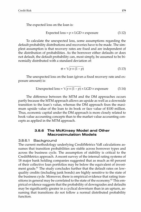
The expected loss on the loan is:

Expected loss = p × LGD × exposure (3.12)

To calculate the unexpected loss, some assumptions regarding thedefault probability distributions and recoveries have to be made. The sim-plest assumption is that recovery rates are fixed and are independent ofthe distribution of probabilities. As the borrower either defaults or doesnot default, the default probability can, most simply, be assumed to be bi-nomially distributed with a standard deviation of:

σ = �p × (1�− p)� (3.13)

The unexpected loss on the loan (given a fixed recovery rate and ex-posure amount) is:

Unexpected loss = �p × (1�− p)� × LGD × exposure (3.14)

The difference between the MTM and the DM approaches occurspartly because the MTM approach allows an upside as well as a downsidetransition to the loan’s value, whereas the DM approach fixes the maxi-mum upside value of the loan to its book or face value of $100 million.Thus, economic capital under the DM approach is more closely related tobook value accounting concepts than to the market value accounting con-cepts as applied in the MTM approach.

3.8.6 The McKinsey Model and OtherMacrosimulation Models

3.8.6.1 BackgroundThe current methodology underlying CreditMetrics VaR calculations as-sumes that transition probabilities are stable across borrower types andacross the business cycle. The assumption of stability is critical to theCreditMetrics approach. A recent survey of the internal rating systems of18 major bank holding companies suggested that as much as 60 percentof their collective loan portfolios may be below the equivalent of invest-ment grade.81 The study concludes further that the default rates on low-quality credits (including junk bonds) are highly sensitive to the state ofthe business cycle. Moreover, there is empirical evidence that rating tran-sitions in general may be correlated to the state of the economy.82 This em-pirical evidence suggests that the probability of downgrades and defaultsmay be significantly greater in a cyclical downturn than in an upturn, as-suming that transitions do not follow a normal distributed probabilityfunction.

Credit Risk 179


3.8.6.2 Incorporating Cyclical FactorsThere are at least two approaches to how to incorporate cyclical factors:

• The past sample period is segregated into recession years andnonrecession years (a recession matrix and a nonrecession matrix)to yield two separate VaR calculations to calculate two separatehistoric transition matrices.

• The Relationship between transition probabilities andmacrofactors is modeled directly, and in a secondary step, amodel is fitted to simulate the evolution of transition probabilitiesover time by shocking the model with macroevents.

McKinsey’s CreditPortfolioView is based on the second approach.

3.8.6.3 The Macrosimulation Multifactor ApproachOne way to build in business cycle effects and to take a forward-lookingview of VaR is to model macroeffects, both systematic and unsystematic,on the probability of default and associated rating transitions. Themacrosimulation approach should be viewed as complementary to Cred-itMetrics, which overcomes some of the biases resulting from assumingstatic or stationary transition probabilities period to period.83

The essential concept is represented in the transition matrix for agiven country, as shown in Figure 3-15. Note especially the cell of the ma-trix in the bottom right-hand corner, pCD.

180 CHAPTER 3

AAAAA

Beginningof period

C

AAA AA C D

End of period

pCD

F I G U R E 3-15

Historic (Unconditional) Transition Matrix.


Each cell in the transition matrix shows the probability that a partic-ular counterparty, rated at a given grade at the beginning of the period,will move to another rating by the end of the period. In Figure 3-15, pCD

shows the estimated probability that a C-rated borrower (in this examplea speculative-grade borrower) will default over the next year—that is, itwill transition from a C rating to a D rating.

In general, it can be expected that this probability moves signifi-cantly during the business cycle and is higher in recessions than in expan-sions. Because the probabilities in each row of the transition matrix mustsum up to 1, an increase in pCD must be compensated for by a decrease inother probabilities—for example, those involving upgrades of initially C-rated debt, where pCB and pCA represent the probabilities of the C-ratedborrower’s moving to, respectively, a B grade and an A grade during thenext year. The probability density in the transition matrix moves increas-ingly in a southeast direction as a recession proceeds.84

With this in mind, let pCD vary at time t along with a set of factors in-dexed by variable y. For convenience, the subscripts C and D will bedropped. However, there is an implicit probability that a C-rated bor-rower will default over the next one-year period. In general terms:85

pt = f(yt) (3.15)

where f < 0

That is, there is an inverse correlation between the state of the econ-omy and the default probability. The macroindicator, variable y, can beviewed as being driven by a set of i systematic macroeconomic variablesat time t (Xit) as well as by unsystematic random shocks, structuralchanges to the economic system such as innovations, new industries andtechnology, and the like. In general:

Yt = g(Xit, Vt) (3.16)

where i = 1, . . . , nVt ∼ N(0, σ)

In turn, macroeconomic variables Xit, such as gross domestic product(GDP) growth, unemployment, and so on, can themselves be consideredto be explained by their past histories (e.g., lagged GDP growth) as well asto be sensitive to shocks themselves, εit.86 Thus:

Xit = h(Xit − 1, Xit − 2 , . . . , εit) (3.17)

Different macromodel specifications can be applied in the context ofEquations (3.16) and (3.17) to improve model fit, and different models canbe used to explain transitions for different countries and industries.

Credit Risk 181


Substituting Equation (3.17) into Equation (3.16), and Equation (3.16)into Equation (3.15), the probability that a speculative grade-C loan willtransition to grade D during the next year will be determined by:

pt = f(Xit − j;Vt, εit) (3.18)

Equation (3.18) models the determinants of this transition probabilityas a function of lagged macrovariables, a general economic shock factor orinnovation Vt, and shock factors or innovations for each of the i macrovari-ables εit. Because the Xit − j are predetermined, the key variables driving pt

will be the innovations or shocks Vt and εit. Using a structured Monte Carlosimulation approach (see Monte Carlo Simulation in Section 5.4.3.5), val-ues for Vt and εit can be generated for periods in the future that occur withthe same probability as that observed from history.87 We can use the simu-lated V and ε values, along with the fitted macromodel, to simulate sce-nario values for pCD in periods t, t + 1, t + 2, . . . , t + n, and on into the future.

Suppose that, based on current macroconditions, the simulatedvalue for pCD, labeled p*, is 0.35, and the number in the historic (uncondi-tional) transition matrix is 0.30 (where the asterisk indicates the simulatedvalue of the transition probability). Because the unconditional transitionvalue of 0.30 is less than the value estimated conditional on the macroeco-nomic state (0.35), we are likely to underestimate the VaR of loans and aloan portfolio, especially at the low-quality end. Defining the ratio rt:

rt = = �00

.

.33

50

� = 1.16 (3.19)

Based on the simulated macromodel, the probability of a C-rated bor-rower’s defaulting over the next year is 16 percent higher than the averageunconditional historical transition relationship implies. We can also calcu-late this ratio for subsequent periods t + 1, t + 2, and so on. For example,suppose that, based on simulated innovations and macrofactor relation-ships, the simulation predicts p*t + 1 to be 0.38. The ratio relevant for thenext year, rt + 1, is then:

rt + 1 = �pp*

t

t

+

+

1

1� = �

00

.

.33

80

� = 1.267 (3.20)

The unconditional transition matrix will underestimate the predicted riskof default on low-grade loans in this period.

These calculated ratios can be used to adjust the elements in the pro-jected t, t + 1, . . . , t + n transition matrices. In McKinsey’s CreditPortfo-lioView, the unconditional value of pCD is adjusted by the ratio of theconditional value of pCD to its unconditional value. Consider the transition

pt*�pt

182 CHAPTER 3


matrix for period t; then rt × 0.30 = 0.35 (which is the same as pt*), thus re-placing 0.30 with 0.35 in the transition matrix pCD, as shown in Figure 3-16.This also means that all the other elements in the transition matrix have tobe adjusted (e.g., pCA, pCB, and so on). A number of procedures can be usedto do this, including linear and nonlinear regressions of each element orcell in the transition matrix on the ratio rt.88 The rows of the transition ma-trix must sum up to 1.89

For the next period (t + 1), the transition matrix would have to besimilarly adjusted by multiplying the unconditional value of p by rt + 1, or0.30 × 1.267 = 0.38. This is shown in Figure 3-17.

Thus, there would be different transition matrices for each year intothe future (t, t + 1, . . . , t + n), reflecting the simulated effect of the macro-economic shocks on transition probabilities. This type of approach, alongwith CreditMetrics, could be used to calculate a cyclically sensitive VaRfor 1 year, 2 years, . . . , n years.90

Specifically, the simulated transition matrix M would replace the his-torically based unconditional (stable Markov) transition matrix, and,given any current rating for the loan (say C), the distribution of loan val-ues based on the macroadjusted transition probabilities in the C row of thematrix Mt could be used to calculate VaR at the one-year horizon, in a fash-ion similar to that used by CreditMetrics in Section 3.8.5.3.

Credit Risk 183

AAAAA

Mt =

C

AAA AAEnd of period

C D

0.35

F I G U R E 3-16

Conditional Transition Matrix Mt.


We could also calculate VaR estimates using longer horizons. Sup-pose we are interested in transitions over the next two years (t and t + 1).Multiplying the two matrices,

Mt′t + 1 = Mt ⋅ Mt + 1 (3.21)

produces a new matrix, Mt′t + 1. The final column of this new matrix willgive the simulated (cumulative) probabilities of default on differentlyrated loans over the next two years.

The macrosimulation approach described until now considered justone simulation of values for p*, from one set of shocks Vt and εit. Thisprocess has to be repeated over and over again—for example, taking10,000 random draws to generate 10,000 estimates of pt* and 10,000 possi-ble transition matrices.

As shown in Figure 3-18, hypothetical simulated values can be plot-ted. The mean simulated value of p* is 0.30, but the extreme value (99thpercentile, or worst-case value) is 0.55. Calculating capital requirementswhen considering unexpected declines in loan values (the latter figure forpt*), and the transition matrix associated with this value, might be consid-ered most relevant for the capital requirement calculation.

184 CHAPTER 3

AAAAA

Mt+1 =

C

AAA AAEnd of period

C D

0.38

F I G U R E 3-17

Conditional Transition Matrix Mt + 1.


3.8.7 KPMG’s Loan Analysis System and Other Risk-Neutral Valuation Approaches

3.8.7.1 BackgroundThe application of risk-neutral probabilities to value risky assets has beenin the finance literature at least as far back as Arrow (1953)91 and has beensubsequently enhanced by Harrison and Kreps (1979),92 Harrison andPliska (1981),93 and Kreps (1982).94 Traditionally, valuing risky assets bydiscounting cash flows is done on an asset by a risk-adjusted discountrate. To do this, the probability distribution for all cash flows and the risk-return preferences of investors have to be known or estimated. The latterare especially difficult to incorporate into the calculation. Suppose that allassets are assumed to trade in a market in which all investors are willingto accept, from any risky asset, the same expected return as that promisedby the risk-free asset. Such a theoretical market can be described as be-having in a risk-neutral fashion. In a financial market in which investorsbehave in a risk-neutral manner, the prices of all assets can be determinedby simply discounting the expected future cash flows on the asset by therisk-free rate.95

The equilibrium relationship, where the expected return on an assetequals the risk-free rate, can be applied to back out an implied risk-neutralprobability of default, also called the equivalent martingale measure. This forward-looking estimate of the default risk of a security can be compared

Credit Risk 185

Prob

abili

ty, %

pt

Expected (mean)value

99th percentile(maximum) value

0 0.1 0.2 0.3 0.4 0.5 0.6

F I G U R E 3-18

Probability Distribution of Simulated Values.


with historical estimated measures of transition probabilities. As long as anasset is risky, the forward-looking risk-neutral probability will not equal itshistorical measure (the realized value of the transition probability).96

3.8.7.2 Deriving Risk-Neutral ProbabilitiesThe following paragraphs discuss two ways of deriving forward-lookingdefault probability measures based on the risk-neutral valuation ap-proach. After that is a discussion of the relationship between the risk-neutral measure of default and its historical measure. The last discussionfocuses on the potential use of the risk-neutral concept in pricing loansand in calculating the market value of a loan and its VaR.

3.8.7.3 Deriving Risk-Neutral Measures from Spreads on Zero-Coupon BondsOne methodology for deriving risk-neutral probabilities from spreads be-tween risky bonds (ratings less than AAA; e.g., corporate bonds) and Trea-suries has been used at Goldman Sachs and was described by Littermanand Iben.97

Consider the two zero-coupon bond yield curves shown in Figure3-19. The annualized discount yield on one-year zero-coupon Treasuriesis assumed to be 10 percent, and the annualized discount yield on one-year grade-B zero-coupon corporates is 15.8 percent. The methodologyassumes that the zero-yield curves either exist or can be fitted. As noted

186 CHAPTER 3

1 2 3 4 Time horizon

Yie

ld

18 %

11 %

15 %

10 %

Zero-coupon corporate bonds (B rating)

Zero-coupon Treasury bonds

F I G U R E 3-19

Comparison of the Zero-Coupon Treasury Bond Curve and the Zero-CouponGrade-B Corporate Bond Curve.


previously, in equilibrium, under risk-neutral valuation, the expected re-turn on the risky bond must equal the risk-free return (the return on therisk-free Treasury bond), or:

p1 × (1 + k1) = 1 + i1 (3.22)

where p1 = implied risk-neutral probability of repayment in year 11 + k1 = expected return on risky one-year corporate bond1 + i1 = risk-free return on one-year Treasury bond

We assume that if the risky bond defaults, the loss given default (LGD)equals 1, and the holder of the bond receives nothing (for simplicity).

From Equation (3.22), we can derive the implied risk-neutral proba-bility of repayment p:

p1 = �11

++

ki 1

1� = �

11.1

.158� = 0.95 (3.23)

Thus, the risk-neutral probability of default p*1 is:

p*1 = 1 − p1 = 1 − 0.95 = 0.05 (3.24)

We can also back out the risk-neutral probability of default in theyear 2, . . . , year n by exploiting the forward rates embedded in the zerocurves in Figure 3-19. For example, p*2, the risk-neutral probability of de-fault in year 2 (essentially, the forward marginal probability that the B-rated corporate borrower will default between year 1 and year 2), can bederived in a two-step process. The first step is to derive the one-year ex-pected forward rates on corporates and Treasuries from the existing zerocurves. The second step is to back out the implied risk-neutral probabil-ity of default from the forward rates. By applying this approach, the en-tire term structure of forward-looking risk-neutral probabilities can bederived.

3.8.7.4 Deriving the Risk-Neutral Probability Measure from Stock PricesUsing bond prices and yield spreads, the preceding approach extractsthe risk-neutral probability of default forecast for a particular borrower(e.g., rate B). This involves placing the borrower into a particular ratingbucket. Thus, this implies a matched yield curve for that rating class andutilizes relationships between zero-coupon bond prices and yields forrisky versus risk-free debt. An alternative approach is to exploit the typeof option-pricing models discussed in Section 2.4.5, along with stockprices and the volatility of stock prices. A risk-neutral probability fore-

Credit Risk 187


cast for a particular borrower can also be backed out of an option-pricingmodel.98 Indeed, from a Merton-type model, where equity is viewed as acall option on the value of the firm’s assets, the probability that the valueof a firm’s assets at the time of debt maturity (e.g., T = 1) will be greaterthan the face value of the firm’s debt is N1(k). The risk-neutral probabil-ity of default is then:

p*t = 1 − N1(k) (3.25)

N1(k) is the area under the normal distribution relating to a variable k,which, in turn, depends on the value of the firm’s assets, the volatility ofthe firm’s assets, leverage, time to maturity, and the risk-free rate. As withthe KMV approach, neither the market value nor the volatility of thefirm’s assets is directly observable. These values have to be iterated fromobservable stock prices and the volatility of stock prices. Delianedis andGeske99 have shown that using the risk-neutral probabilities derived froma standard Merton model100 as a first step and the risk-neutral probabili-ties derived from an enhanced Merton-type model101 as a second step al-lows for multiple classes of debt, demonstrating the ability of thesemeasures to predict actual rating transitions and defaults. In other words,the risk-neutral measure has the potential to predict changes in the histor-ical measure.102

3.8.7.5 The Relationship Between the Historical and the Risk-Neutral MeasuresFollowing Ginzberg et al.103 and Belkin et al.,104 the relationship betweenthe risk-neutral measure and the historical measure of default probabilitycan be best viewed in terms of a risk premium.105 That is, the spread Φ be-tween the returns on a one-year risk-free asset (such as a corporate bond)will reflect the risk-neutral probability of default p*1 and some loss givendefault (LGD):

Φ1 = p*1 × LGD (3.26)

Alternatively, we can view the spread as compensating investors forboth an expected loss ε1 and an unexpected loss u1 on the risky bond:

Φ1 = ε1 + u1 (3.27)

The expected loss ε1 can, in turn, be set equal to the average or his-torical probability of default of this type of borrower by multiplying thehistoric transition probability t1 times the LGD:106

ε1 = t1 × LGD (3.28)

188 CHAPTER 3


The unexpected loss component u1 can be viewed as being equal to theunexpected default probability of default times the LGD.107

Substituting Equation (3.28) into Equation (3.27) and incorporatingEquation (3.26) results in:

p*1 × LGD = (t1 × LGD) + u1 (3.29)

Given some fixed LGD, the difference between p* (the risk-neutralprobability of default) and t1 (the historical probability of default) is a riskpremium that reflects the unexpected default probability. For example, ifΦ = 1 percent, LGD = 40 percent, and t1 = 1 percent, then:

Φ1 = p*1 × LGD = (t1 × LGD) + u1 (3.30)

Φ1 = p*1 × 0.40 = (0.01 × 0.40) + u1 = 0.01 (3.31)

In the next step we solve for values of both p*1 and u1. From Equations(3.30) and (3.31), the risk-neutral probability of default p*1 = 2.5 percent,which is higher than the historical default probability of t1 = 1 percent, andthe unexpected loss or risk premium u1 = 0.60 percent.

Ginzberg et al.108 offer an approach to how actual U.S. credit spreadscan be segregated into an expected loss and a risk premium component.For example, an average (par) spread of 20.01 basis points on one-yearAAA corporates over one-year Treasuries can be broken down into an ex-pected loss component t1 × LGD of 0.01 basis points and a risk premiumu1 of 20 basis points. An 1188.97 basis-point spread on one-year CCCbonds over Treasuries can be broken down into an expected loss compo-nent of 918.97 basis points and an unexpected loss component of 270basis points.

3.8.7.6 Risk-Neutral Probabilities Applied to Credit Risk ValuationRisk-neutral probabilities offer substantial potential value for a credit offi-cer in pricing decisions and in making market valuations of loans. For ex-ample, risk-neutral probabilities can be used in setting the required spreador risk premium on a loan. Following Ginzberg et al.,109 assume a credit of-ficer wants to find the fixed spread W on a one-year loan that will yield $1of expected NPV from each $1 lent. The loan would be a break-even proj-ect in an NPV sense. The credit officer knows that:

• r = one-year risk-free rate = 4 percent• p*1 = risk-neutral probability of default = 6.5 percent• LGD = 33.434 percent

Credit Risk 189


To solve for s:

E(NPV) = (1 − p*1)(1 + r + s) + p*1(1 − LGD)1 + r

= (0.935)(1.04 + s) + 0.65(0.66566)1.04

(3.32)

The value of the loan spread s that solves Equation (3.32) is 2.602 per-cent. However, a major problem with this approach is seen in extendingthis type of analysis beyond the one-year horizon. The default or no-default scenario, under which risk-neutral probabilities are derived, fitsthe one-year loan case but not the multiyear loan case. For multiyearloans, a richer universe of possibilities exists. These include borrower mi-gration upgrades and downgrades, which may trigger some loan repric-ing clauses, which may in turn affect the value of the loan and theborrower’s option to prepay a loan early.

Ginzberg et al.110 and KPMG’s Loan Analysis System111 have at-tempted to extend the valuation framework in Equation (3.32) to multi-period loans with a variety of options. These options include loan spreadrepricing as nondefault transitions in credit quality occur and building inpenalty fees for borrowers who prepay early.

Figure 3-20, from Aguis et al.,112 describes, in a simplified fashion, thepotential transitions of the credit rating of a B-rated borrower over a four-year loan period. Similarities with bond valuation models, especially lat-tice or “tree” diagrams for bond valuation (binominal model), are obvious.Given transition probabilities, the original grade-B borrower can migrateup or down over the loan’s life to different ratings, and may even defaultand migrate to D (an absorbing state). Along with these migrations, a pric-ing grid that reflects the bank’s current policy on spread repricing for bor-rowers of different quality can be built. This methodology has the potentialto generate additional information regarding whether the credit model hasa good or bad repricing grid in an expected NPV sense—basically, whetherE(NPV) ≠ 1.

When valuing a loan in this framework, valuation takes place recur-sively (from right to left in Figure 3-20), as it does when valuing bondsunder binomial or multinomial models. For example, if the E(NPV) of theloan in its final year is too high (too rich), and given some prepayment fee,the model supports prepayment of the loan to take place at the end of pe-riod 3. Working backward through the tree from right to left, the totalE(NPV) of the four-year loan can be calculated. Moreover, the credit offi-cer can make different assumptions about spreads (the pricing grid) andprepayment fees to determine the loan’s value. Other parameters of a

190 CHAPTER 3


loan’s structure, such as caps, and amortization schedules, can be built in,and a VaR can be calculated.113

The risk-neutral valuation framework supports the calculation forboth default prediction and loan valuation. Compared to historic transi-tion probabilities, the risk-neutral model gives the advantage of a forward-looking prediction of default. The risk-neutral prediction willgenerally exceed the history-based transition prediction over some hori-zon because, conceptually, it contains a risk premium reflecting the unex-pected probability of default. Moreover, the risk-neutral frameworkconsiders only two credit states: default and nondefault; it does not recog-nize several rating buckets.

KPMG suggested a valuation approach that is potentially consistentwith the risk-neutral model under no arbitrage.114 Over its life, a loan canmigrate to states other than default/nondefault. The valuation model issimilar in spirit to a multinomial tree model for bond valuation, with thedifference that transition probabilities replace interest-rate movementprobabilities. This model has some flexibility, as credit spreads can vary,fees can be charged on prepayments, and other special provisions can be

Credit Risk 191

Grade x

Grade 3

Grade 2

Grade 1

Grade n

Grade 3

Grade 2

Grade 1

Grade n

Grade 3

Grade 2

Grade 1

Grade n

Time horizon t1 2 3 4

. . .

AA to A

AAA toAA

Default

EDFs for multiperiod loan migrations Risk grade

F I G U R E 3-20

Multiperiod Loan Transitions Over Many Periods. [Source: Scott D. Aguais andAnthony M. Santomero, “Incorporating New Fixed Income Approaches into Com-mercial Loan Valuation,” Journal of Lending and Credit Risk Management 80/6(February 1998), 58–65, fig. 2, http://fic.wharton.upenn.edu/fic/papers/98.html.Reproduced with permission of the authors.]


built into the valuation process. A question arises as to the link betweenthe model and the existence of an underlying portfolio of replicating as-sets. In particular, the exact details of the construction of a replicating no-arbitrage portfolio for a multiperiod nontradable loan are still open.

3.8.8 The CSFB CreditRisk+ Model

3.8.8.1 BackgroundOnly quite recently have ideas and concepts from the insurance industryfound their way into the new approaches for credit risk measurement andmanagement. The following sections discuss two applications of insur-ance ideas, one from life insurance and one from property insurance. Alt-man115 and others have developed mortality tables for loans and bondsusing ideas (and models) similar to those that insurance actuaries usewhen they set premiums for life insurance policies. Credit Suisse FinancialProducts, a former subsidiary of Credit Suisse First Boston (CSFB), devel-oped a model similar to the one used by household insurance vendors forassessing the risk of policy losses in setting premiums.

3.8.8.2 Migration of Mortality Approach for Credit Risk MeasurementThe concept is quite simple: based on a portfolio of loans or bonds andtheir historic default experience, develop a table that can be applied in apredictive sense for one-year or marginal mortality rates (MMRs) and formultiyear or cumulative mortality rates (CMRs). Combining such calcu-lations with LGDs allows us to create estimates of expected losses.116

To calculate the MMRs of a B-rated bond or loan defaulting in eachyear of its life, the analyst will pick a sample of years—say, 1971 through1998—and, for each individual year, will analyze:

MMR1 =Total value of grade-B bonds defaulting in year 1 of issueTotal value of a B-rated bond outstanding in year 1 of issue

MMR2 =Total value of B-rated bond defaulting in year 2 of issueTotal value of a B-rated bond outstanding in year 2 of issue (adjusted for defaults, calls, sinking fund redemptions, and maturities in the prior year) (3.33)

And so on for MMR3, . . . , MMRn.When the MMR for a specific individual year has been calculated,

the credit officer calculates a weighted average of all MMRs, which be-comes the figure entered into the mortality table. The weights used should

192 CHAPTER 3


reflect the relative issue sizes in different years, thus biasing the resultstoward the years with larger issues. The average MMR in year 1 for a par-ticular rating bucket (M�M�R�) would be calculated as:

M�M�R�1 = �1998

i = 1971

MMR1i ⋅ wi

� wi = 1 (3.34)

To calculate a CMR—the probability that a loan or bond will defaultover a period longer than a year (e.g., 2 years)—it is first necessary to spec-ify the relationship between MMRs and survival rates (SRs):

MMRi = 1 − SRi

SRi = 1 − MMRi (3.35)

Consequently,

CMRN = 1 − �N

i = 1SRi (3.36)

where ∏ is the geometric sum or product [SR1 × SR2 × . . . SRN] and N de-notes the number of years over which the cumulative mortality rate iscalculated.

3.8.8.3 Mortality Rates and TablesTable 3-7 shows MMRs and CMRs for syndicated loans and bonds over afive-year horizon, as computed by Altman and Suggitt.117 Looking at thetable in more detail, we can see that for the higher-grade buckets the mor-tality rates are quite comparable, but this is not the case for the lowest-quality-rating buckets. For example, low-quality loans have substantiallyhigher MMRs in the first three years of life than do similarly rated bonds.The critical question is whether high-yield loans and bonds have sub-stantially different default profiles, or is this a statistical result due to arelatively small sample size? In particular, although not described, eachof the MMR estimates has an implied standard error and confidence in-terval. It can be shown that with an increasing number of loans or bondsin the observation sample (i.e., as n gets bigger), the standard error on amortality rate will fall (i.e., the degree of confidence level applied to cal-culate the MMR estimate of expected out-of-sample losses increases). Asa loan or bond either dies or survives in any period, the standard error Tof an MMR is:118

Credit Risk 193


194

TA

BL

E3- 7

Com

paris

on o

f Syn

dica

ted

Ban

k Lo

an V

ersu

s C

orpo

rate

Bon

d M

orta

lity

Rat

es, B

ased

on

Orig

inal

Issu

ance

Prin

cipa

l Am

ount

s (1

991

–19

96)

Year

s af

ter I

ssue

12

34

5

Rat

ing

Ban

kB

on

dB

ank

Bo

nd

Ban

kB

on

dB

ank

Bo

nd

Ban

kB

on

d

AA

A Mar

gina

l0.

00%

0.00

%0.

00%

0.00

%0.

00%

0.00

%0.

00%

0.00

%0.

00%

0.00

%C

umul

ativ

e0.

000.

000.

000.

000.

000.

000.

000.

000.

000.

00A

a Mar

gina

l0.

000.

000.

000.

000.

000.

000.

000.

000.

000.

00C

umul

ativ

e0.

000.

000.

000.

000.

000.

000.

000.

000.

000.

00A

Mar

gina

l0.

000.

000.

120.

000.

000.

000.

000.

000.

000.

05C

umul

ativ

e0.

000.

000.

120.

000.

120.

000.

120.

000.

120.

05B

aa Mar

gina

l0.

040.

000.

000.

000.

000.

000.

000.

540.

000.

00C

umul

ativ

e0.

040.

000.

040.

000.

040.

000.

040.

540.

040.

54B

a Mar

gina

l0.

170.

000.

600.

380.

602.

300.

971.

804.

890.

00C

umul

ativ

e0.

170.

000.

770.

381.

362.

672.

324.

427.

104.

42B

Mar

gina

l2.

300.

811.

861.

972.

594.

991.

791.

761.

860.

00C

umul

ativ

e2.

300.

814.

112.

766.

607.

618.

279.

249.

979.

24C

aa Mar

gina

l15

.24

2.65

7.44

3.09

13.0

34.

550.

0021

.72

0.00

0.00

Cum

ulat

ive

15.2

42.

6521

.55

5.66

31.7

79.

9531

.77

29.5

131

.77

29.5

1

SO

UR

CE:

E.I

.Altm

an a

nd H

.J.S

uggi

tt, “

Def

ault

Rat

es in

the

Syn

dica

ted

Loan

Mar

ket:

A M

orta

lity

Ana

lysi

s,”W

orki

ng P

aper

S-9

7-39

, Ne w

Yor

k U

nive

rsity

Sal

omon

Cen

ter,

New

Yor

k, D

ecem

ber

1997

.R

epro

duce

d w

ith p

erm

issi

on o

f NY

U S

alom

on C

ente

r .


σ = (3.37)

and rearranging:

N = (3.38)

As can be derived from Equations (3.37) and (3.38), there is an in-verse relationship between sample size N and the standard error σ of amortality rate estimate.

Assume that MMR1 = 0.01 is a mortality rate estimate, and extremeactuarial standards of confidence in the stability of the estimate for pricingand prediction out of sample have to be applied. Extreme actuarial stan-dards might require σ to be one-tenth the size of the mortality rate esti-mate (or σ = 0.001). Plugging these values into Equation (3.38) results in:

N = �(0.0

(01.)0⋅0(10).2

99)� = 9900 (3.39)

This results in 10,000 loan observations per rating bucket required toobtain this type of confidence in the estimate. With, say, 10 rating classes, aportfolio of some 100,000 loans would have to be analyzed and calculated.Very few banks have the resources to build information systems of this type.To get to the requisite large size, a nationwide effort among the banks them-selves may be required. The end result of such a cooperative effort might bea national loan mortality table per country that could be used for the calcu-lation of the banks’ loan loss reserves, based on expected losses, similar tothe national life mortality tables applied in pricing life insurance.119

3.8.9 CSFB’s CreditRisk+ Approach

This section analyzes two insurance-based approaches to credit risk analysis.Mortality analysis offers an actuarial approach to predicting default rates,which is considered an alternative to some of the traditional accounting-based models for measuring expected losses and loan loss reserves. Theadded value of mortality rates very much depends on the size of the sampleof loans or bonds from which they are calculated. CreditRisk+, an alternativeto CreditMetrics, calculates capital requirements based on actuarial ap-proaches found in property insurance concepts. The major advantage is therather minimal data input required (e.g., no data on credit spreads are re-quired). Its major limitation is that it is not a full VaR model because it fo-cuses on loss rates rather than loan value changes. It is a default-mode (DM)model rather than a mark-to-market (MTM) model.

MMRi ⋅ (1 − MMRi)��

σ2

MMRi ⋅ (1 − MMRi)��

N

Credit Risk 195


The approach developed by CSFB stands in direct contrast to Credit-Metrics in its objectives and its theoretical framework:

• CreditMetrics seeks to estimate the full VaR of a loan or loanportfolio by viewing rating upgrades and downgrades and theassociated effects of spread changes in the discount rate as part ofthe credit’s VaR exposure. In contrast, CreditRisk+ considersspread risk as part of market risk rather than credit risk. As aresult, in any period, only two states of the credit world areconsidered, default and nondefault. The focus is on measuringexpected and unexpected losses rather than expected value andunexpected changes in value (or VaR) as under CreditMetrics. Asmentioned, CreditMetrics is an MTM model, whereas CreditRisk+

is a DM-based model.• The second major conceptual difference is that in CreditMetrics,

the default probability in any year is modeled based on a discreteassumption (as are the upgrade/downgrade probabilities). InCreditRisk+, default is modeled as a continuous variable with aprobability distribution. An analogy from home insurance isrelevant. When a whole portfolio of home loans is insured, there isa small probability that all houses will burn down simultaneously.In general, the probability that each house will burn down can beconsidered as an independent event. Similarly, many types ofloans, such as mortgages and small business loans, can beanalyzed in a similar way, with respect to their default risk. In theCreditRisk+ model, each individual loan is assumed to have asmall default probability, and each loan’s default probability isindependent of the default on other loans.120 This assumption ofindependent occurrence makes the default probability distributionof a loan portfolio resemble a Poisson distribution.

Figure 3-21 presents the difference in assumptions regarding defaultprobability distribution in CreditRisk+ and CreditMetrics.

The two degrees of uncertainty, the default frequency and the lossseverity, produce a distribution of losses for each exposure band. Sum-ming (or, more exactly, aggregating) these losses across exposure bandsproduces a distribution of losses for the loan portfolio (Figure 3-22). Al-though not labeled by CSFB as such, we shall call the model in Figure 3-23Model 1. The computed loss function, assuming a Poisson distribution forindividual default rates and the bucketing of losses, is displayed in Figure3-23. The loss function is quite symmetric and is close to the normal dis-tribution, which it increasingly approximates as the number of loans inthe portfolio increases. However, as discussed by CSFB, default and lossrates tend to have fatter tails than is implied by Figure 3-23.121 Specifically,the Poisson distribution implies that the mean default rate of a portfolio ofloans should equal its variance, that is:

196 CHAPTER 3


σ2 = mean (3.40)

σ = �mean� (3.41)

Using figures on default rates from Carty and Lieberman,122 CSFB showsthat, in general, Equation (3.41) does not hold, especially for lower-qualitycredit. For B-rated bonds, Carty and Lieberman found that the mean de-fault rate was 7.27 percent, its square root was 2.69 percent, and its σ was

Credit Risk 197

Time horizon

Def

ault

rate

Def

ault

rate

Possible paths of default rate

Credit Risk Plus

BBB loan

o

Time horizon

Possible paths of default rate

BBB loan

CreditMetrics

AAA

. . .

BBB

. . .

Default

o

F I G U R E 3-21

Comparison of the CreditRisk+ and CreditMetrics Models.


5.1 percent, or almost twice as large as the square root of the mean (seeFigure 3-23). This answers the question of what extra degree of uncer-tainty might explain the higher variance (fatter tails) in observed loss dis-tributions. The additional uncertainty modeled by CSFB is that the meandefault rate itself can vary over time or over the business cycle. For exam-ple, in economic expansions, the mean default rate will be low; in eco-

198 CHAPTER 3

Default loss

Prob

abili

ty

Frequency of defaults Severity of loss

Distribution of default losses

F I G U R E 3-22

Influencing Factors on Distribution of Losses.

Loss

Prob

abili

ty

Model 1

Actual loss distribution

F I G U R E 3-23

Distribution of Credit Losses with Default Rate Uncertainty and Severity Uncertainty.


nomic contractions, it may rise substantially. In their extended model(henceforth called Model 2), there are three types of uncertainty:

• The uncertainty of the default rate around any given meandefault rate

• The uncertainty about the loss severity• The uncertainty about the mean default rate itself, modeled as a

gamma distribution by CSFP123

Appropriately implemented, a loss distribution can be calculatedalong with expected losses and unexpected losses that exhibit observ-able fatter tails. The latter can then be used to calculate the capital re-quirement, as shown in Figure 3-24. Note that this economic capitalmeasure is comparable with the VaR measured under CreditMetrics, be-cause CreditMetrics allows for rating upgrades and downgrades that af-fect a loan’s value. By contrast, there are no nondefault migrations in theCSFB model. Thus, the CSFB capital calculation is closer to a loss-of-earnings or book-value capital measure than a full market value of eco-nomic capital measure. Nevertheless, its great advantage lies in itsparsimonious requirement of data. The key data inputs are mean lossrates and loss severities, for various loss buckets in the loan portfolio,both of which are potentially amenable to collection, either internally orexternally. A simple discrete example of the CSFB Model 1 will illustratethe minimal data input that is required.

Credit Risk 199

Loss

Prob

abili

ty

Economic capital

Unexpected loss at 99th percentile level

Expected loss

Uncovered losses

F I G U R E 3-24

Capital Requirement Based on the CSFB CreditRisk+ Model.


3.8.10 Summary and Comparison of New Internal Model Approaches

3.8.10.1 BackgroundThe previous sections describe key features of some of the more prominentnew quantitative models of credit risk measurement that are publicly avail-able. At first glance, these approaches appear to be very different and likelyto generate substantially different loan loss exposures and VaR measures.The following sections summarize and compare four of these new modelsand highlight key differences and similarities among them.

3.8.10.2 Model ComparisonSix key dimensions are used to compare the different approaches amongthe four models: (1) CreditMetrics, (2) CreditPortfolioView, (3) Cred-itRisk+, and (4) KMV. Analytically and empirically, these models are not asdifferent as they may first appear. Indeed, similar arguments have beenmade by Gordy,124 Koyluoglu and Hickman,125 and Crouhy and Mark,126

using different model anatomies. Table 3-8 displays the six key dimen-sions for comparing the models.

200 CHAPTER 3

T A B L E 3-8

Comparison of Different Approaches

Model

Dimensions CreditPortfolio-for CreditMetrics View CreditRisk+

Comparison (J. P. Morgan) (McKinsey) (CSFP) KMV

Definition of MTM MTM or DM DM MTM or DMrisk

Risk drivers Asset values Macrofactors Expected Asset valuesdefault rates

Volatility of Constant Cyclical Variable Variablecredit events

Correlations of Multivariate Factor loadings Conditional Multivariatecredit events normal asset correlation of independence normal asset

returns residual risk assumption or returnscorrelation with expected default rate

Recovery Random Random Constant with Constant or rates buckets random

Numerical Simulation or Simulation Closed-form Closed-form approach analytic (one- (one-period solution solution

period VaR) VaR)


3.8.10.3 Definition of Risk in the Different ModelsAs described in the previous sections, we distinguish between models thatcalculate VaR based on the change in the market value of loans usingmark-to-market (MTM) models, and models that focus on predicting de-fault losses using default-mode (DM) models.127 The MTM models allowfor credit upgrades and downgrades, and therefore spread changes, aswell as defaults in calculating loan value losses and gains. Contrarily, theDM models consider only two states of the credit world: default and non-default. The key difference between the MTM and DM approaches is theinclusion of spread risk in MTM models. Not surprisingly, if models in-corporate different input, they are likely to produce different results.CreditMetrics is an MTM model, whereas CreditRisk+ and KMV are DMmodels. CreditPortfolioView can be implemented as an MTM or a DMmodel.

3.8.10.4 Risk DriversCreditMetrics and KMV have their analytic foundations in a Merton-typemodel; a firm’s asset values and the volatility of asset values are the keydrivers and input variables of default risk. In CreditPortfolioView, the riskdrivers are macrofactors (such as inflation, credit spread, etc.); in Credit-Risk+, the risk drivers are the mean level of default risk and its volatility. Ifexpressed in terms of multifactor models, all four models can be viewed ashaving similar roots.128 Specifically, the variability of a firm’s asset returnsin CreditMetrics (as well as in KMV) is modeled as being directly linked tothe variability in a firm’s stock returns. In calculating correlations amongfirms’ asset returns, the stocks of individual firms are determined by a setof systematic risk factors (industry factors, country factors, etc.) and un-systematic risk factors. The systematic risk factors, along with correlationsamong systematic risk factors (and their weighted sensitivity, similar tothe multifactor/arbitrage pricing theory of model portfolio theory), deter-mine the asset returns of individual firms and the default correlationsamong firms.

The risk drivers in CreditPortfolioView have methodological foun-dations similar to those of CreditMetrics and KMV. In particular, a set oflocal systematic market macrofactors and unsystematic macroshocksdrives default risk and the correlations of default risks among borrowersin the same local market. The key risk driver in CreditRisk+ is the variablemean default rate in the economy. This mean default rate can be linked sys-tematically to the state of the macroeconomy—when the macroeconomydeteriorates, the mean default rate is likely to rise, as are default losses.Improvement in economic conditions has the opposite effect.

Risk drivers and correlations in all four models can be correlated toa certain extent to macrofactors describing the evolution of economywideconditions.

Credit Risk 201


3.8.10.5 Volatility of Credit EventsA key difference in the methodology among the models is in the modelingof the one-year default probability or the probability of default distribu-tion function. In CreditMetrics, the default probability (as well as up-grades and downgrades) is modeled as a fixed or discrete value based onhistoric data. In KMV, expected default frequencies (EDFs) are linked tothe variability of the firm’s stock returns, and will vary as new informa-tion is impounded in stock prices. Variations in stock prices and thevolatility of stock prices determine the KMV’s EDF scores. In CreditPort-folioView, the default probability is a logistic function of a set of macro-factors and normally distributed shocks. As the macroeconomy evolves,the default probability and the cells, or probabilities, in the rest of the tran-sition matrix will evolve as well. In CreditRisk+, the default probability ofeach loan is assumed to be variable, following a Poisson distributionaround some mean default rate. The mean default rate is modeled as avariable with a gamma distribution. This produces a distribution of lossesthat may have fatter tails than those produced by either CreditMetrics orCreditPortfolioView.

3.8.10.6 Correlation of Credit EventsThe similarity of the determinants of credit risk correlations has been dis-cussed in the context of risk drivers. Specifically, the correlation structurein all four models can be attributed to systematic sensitivities of loans tokey factors. The correlations among borrowers are discussed in Section3.9.6, where the application of the new models and modern portfolio the-ory to support credit portfolio decisions is discussed.

3.8.10.7 Recovery RatesThe loss distribution and VaR calculations depend not only on the defaultprobability but also on the loss severity or loss given default (LGD). Em-pirical evidence suggests that default severities and recovery rates arequite volatile over time. More precisely, building in a volatile recovery rateis likely to increase the VaR or unexpected loss rate.

CreditMetrics, in the context of its VaR calculations, allows for re-coveries to be variable. In the current model version, which recognizes askew in the tail of the loan value loss distribution function, recovery ratesare assumed to follow a beta distribution, and the VaR of loans is calcu-lated via a Monte Carlo simulation. In KMV’s simplest model, recoveryrates are considered constant over time. In more recent extended versionsof the model, recovery rates are allowed to follow a beta distribution aswell. In CreditPortfolioView, recovery rates are also estimated via a MonteCarlo simulation approach. By contrast, under CreditRisk+, loss severitiesare clustered and allocated into subportfolios, and the loss severity in anysubportfolio is considered constant over time.

202 CHAPTER 3


3.8.10.8 Numerical ApproachThe estimation approach of VaRs, or unexpected losses, differs acrossmodels. A VaR, at both the individual loan level and the loan portfoliolevel, can be calculated analytically under CreditMetrics. This approachbecomes increasingly intractable as the number of loans in the portfolioincreases. As a result, for large loan portfolios, Monte Carlo simulationtechniques are applied to generate an approximate aggregate distributionof portfolio loan values, and thus a VaR. Similarly, CreditPortfolioViewuses repeated Monte Carlo simulations to generate macroshocks and thedistribution of losses (or loan values) of a loan portfolio. CreditRisk+,based on its convenient distributional assumptions (the Poisson distribu-tion for individual loans and the gamma distribution for the mean defaultrate, along with the fixed recovery assumption for loan losses in each sub-portfolio of loans), allows an analytic or closed-form solution to be gener-ated for the probability density function of losses. KMV allows an analyticsolution to the loss function.

The development of internal models for credit risk measurementand capital requirements is at an early stage. In some sense, its presentlevel of development can be compared to that of market risk in 1994, whenRiskMetrics first appeared and was followed by alternative methodolo-gies such as historic simulation and Monte Carlo simulation. The creditrisk models publicly available to date have exhibited quite different ap-proaches across a number of important dimensions. Harmonizing thesemodels across just a few key dimensions, however, can result in quitecomparable unexpected loss calculations. This suggests that over time,with theoretical and model development, a consensus model or approachmay eventually emerge. To some extent, this has already happened in themarket risk modeling area, supported by regulatory incentives.

3.8.11 Comparison of Major Credit Risk ModelsA variety of credit models exists, which are mainly portfolio approaches.The different conceptual approaches of the most current applications aresummarized in the following list:

• KMVConceptual model. Expected default frequency based on marketvalue of assets. Borrower defaults when available resources havebeen depleted below a critical level. EDFs are linked to thevariability of the firm’s stock returns, which will vary as newinformation is impounded in stock prices. Variations in stock pricesand the volatility of stock prices determine the KMV stock scores.Modeling of concentration. A multifactor stock return model isapplied, from which correlations are calculated. The modelreflects the correlation among the systemic risk factors affecting

Credit Risk 203


each firm’s asset correlation, their individual defaultprobabilities, and their appropriate weights. The approach toestimate correlations is similar to that used in CreditMetrics.However, KMV typically finds that correlations lie in the range of0.002 to 0.15, which is relatively low.

• CreditMetricsConceptual model. Simulation-based portfolio approach, in whichchanges in debt values are modeled based on changes in rating,and the market value of each position is a derived function of itsrating. Simulations of credit migrations are time consuming.Modeling of concentration. Concentration risk is modeled bysector allocation, and borrower correlation is derived from sectorcorrelations. Asset returns are simulated and mapped tosimulated credit migrations. Recovery rates are random variables.

• CreditRisk+

Conceptual model. Insurance or actuarial type for modeling low-probability, high-impact events. Default probability of each loanis assumed to be a random, conditionally independent variable,following a Poisson distribution around some mean default rate.The mean default rate is modeled as a variable with a gammadistribution. The default probability on each sector is different.Modeling of concentration. Each position is allocated to sectorsthat represent countries and industries. Sectors are conditionallyassumed to be independent, and one individual sector can beused for modeling the specific risk of positions.

• CreditPortfolioViewConceptual model. A conditioned transition matrix is calculated,simulating the evolution of transition probabilities over time bygenerating macroshocks to the model. The simulated transitionmatrix replaces the historically based unconditional (stableMarkov) transition matrix. Given any current rating for the loan,the distribution of loan values, based on the macroadjustedtransition probabilities in the row for a specific rating of thematrix, could be used to calculate VaR at the one-year horizon, ina fashion similar to that used in CreditMetrics. A cyclicallysensitive VaR for 1, 2, . . . , n years can be calculated.Modeling of concentration. Directly models the relationship betweentransition probabilities and macrofactors; in a secondary step, amodel is fitted to simulate the evolution of transition probabilitiesover time by shocking the model with macroevents. Each position isallocated to sectors that represent countries and industries. Sectorsare not conditionally assumed to be independent.

204 CHAPTER 3


Depending on the conceptual approach of the model, the input pa-rameters are different, as is the way some of the key elements of credit riskare handled. Correlations that are inferred from equity indexes (such asthe CreditMetrics model) require a three-step process for the computationof the credit correlation coefficient (Figure 3-25):

• CreditMetrics provides the correlation coefficients describing thecomovements of various industry–country equity indexes.

• The user has to define (input) how much of the variance in anindividual borrower’s credit indicator is derived from the variouscountry–industry indexes.

• The model then computes the borrower’s credit correlationcoefficients.

Volatility values are critical information for the portfolio approach,as they are the basis for the correlation calculation, a key component of theportfolio approach. To measure portfolio VaR, one starts with the loan-

Credit Risk 205

Currentvaluation

BBB

BB

BBB

A

5%

88%

5%

1%

Transition rates Forward values

D

AAA

AA

0.6%

0.1%

0.2%

0.1%

99.8

100.07

100.1

92

99.1

70

100.1

100.1

Expectedvalue 100.0

Standardvaluation

1.04

Volatility depends on position pricing andinstrument structure as well as transition

Output

C

B

F I G U R E 3-25

Three-Step Process for Calculation of Credit Correlation Coefficients.


specific volatility, which reflects price (historical and future) and the struc-ture of the loan. The volatility depends on the issue of price and structureas well as the transitions. The forward valuation depends on:

• Loan price and loan structure• Collateral• Spread and fees• Amortization• Tenor• Options (e.g., prepayment, repricing or grid, term-out, and market

conditions)The portfolio distribution can be produced by simulation, using ran-

dom draws of the loans’ xi values. In a second step, the end-of-period rat-ings are derived. In a third step, the loans are priced, based on the ratingsand other input parameters. In a fourth step, the loans are summed up toget the portfolio value by using the values and the correlation from therandom draws. This procedure is repeated many times to derive a stabledistribution of the portfolio with the loans’ xi values (see Figure 3-26).

Instead of estimating the loans’ xi values, the distribution of commonand specific factors can be estimated by using random draws of the fac-tors. In a first step, random draws of the factors are taken. In a second step,the random draws of the factors are used to calculate the xi values. In athird step, the loans are priced, based on the ratings and other input pa-rameters. In a fourth step, the loans are summed up to get the portfoliovalue by using the values and the correlation from the random draws.This procedure is repeated many times to derive a stable distribution ofthe portfolio with the loans’ xi values (see Figure 3-27).

206 CHAPTER 3

AAA AA A BBB BB B CCC DLoan x 106.1 106.1 106.1 106.07 105.7 105.1 98.0 70Loan x 106.0 106.05 106.05 106.0 105.95 104.40 100.9 72

211.70

1. Draw xi

2

2

1

1

2. Derive end-of-period ratings

3. Price loan based on rating

4. Sum to getportfolio value

105.70

5. Repeat

x

x

BBBBBBCCC A AAD AAA

F I G U R E 3-26

Computation of Portfolio Distribution Through Simulation Process.


3.9 MODERN PORTFOLIO THEORY AND ITSAPPLICATION TO LOAN PORTFOLIOS

3.9.1 Background

Default risk and credit risk exposure are commonly viewed on a single-borrower basis. Much of the banking theory literature views the personnelat banks and similar institutions as credit specialists who, over time,through monitoring and the development of long-term relationships withcustomers, gain a comparative advantage in lending to a specific bor-rower or group of borrowers. (The current BIS risk-based capital ratio islinearly additive across individual loans.) This advantage, developed bygranting (and holding to maturity) loans to a select subset of long-termborrowers, can be viewed as inefficient from a risk–return perspective. In-stead, loans publicly traded, or “swappable” with other financial organi-zations, could be considered as being similar to commodity-type assetssuch as equities, which are freely traded at low transaction costs and withhigh liquidity in public securities markets. By separating the credit-grant-ing decision from the credit portfolio decision, a financial organizationmay be able to generate a better risk–return trade-off, and offset whatKMV and others have called the paradox of credit.

Figure 3-28 illustrates the paradox of credit by applying the efficientfrontier approach to loans. Portfolio A is a relatively concentrated loan

Credit Risk 207

BBBBBBCCC A AAD AAA

AAA AA A BBB BB B CCC DLoan x 106.1 106.1 106.1 106.07 105.7 105.1 98.0 70Loan x 106.0 106.05 106.05 106.0 105.95 104.40 100.9 72

211.70

1. Draw x i

3. Derive end-of-period ratings

4. Price loan based on rating

5. Sum to get portfoliovalue

105.70

6. Repeat

F ( Y

)

Y

F ( Z

)

Z

2. Insert to form x si

Zy1x

Zy1x

22

11

2

1

⋅ρ+⋅ρ-=

⋅ρ+⋅ρ-=

F I G U R E 3-27

Distribution of Common and Specific Factors Through Random Drawing.


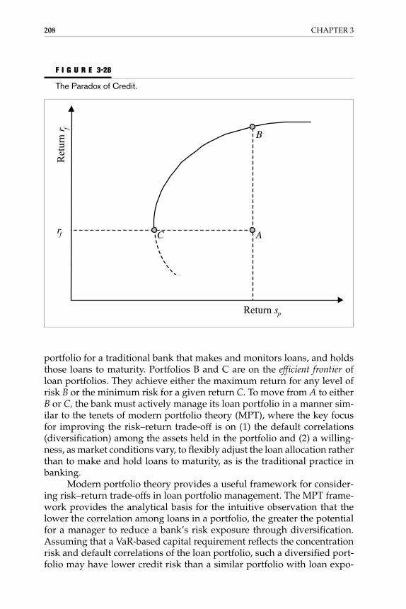
portfolio for a traditional bank that makes and monitors loans, and holdsthose loans to maturity. Portfolios B and C are on the efficient frontier ofloan portfolios. They achieve either the maximum return for any level ofrisk B or the minimum risk for a given return C. To move from A to eitherB or C, the bank must actively manage its loan portfolio in a manner sim-ilar to the tenets of modern portfolio theory (MPT), where the key focusfor improving the risk–return trade-off is on (1) the default correlations(diversification) among the assets held in the portfolio and (2) a willing-ness, as market conditions vary, to flexibly adjust the loan allocation ratherthan to make and hold loans to maturity, as is the traditional practice inbanking.

Modern portfolio theory provides a useful framework for consider-ing risk–return trade-offs in loan portfolio management. The MPT frame-work provides the analytical basis for the intuitive observation that thelower the correlation among loans in a portfolio, the greater the potentialfor a manager to reduce a bank’s risk exposure through diversification.Assuming that a VaR-based capital requirement reflects the concentrationrisk and default correlations of the loan portfolio, such a diversified port-folio may have lower credit risk than a similar portfolio with loan expo-

208 CHAPTER 3

Ret

urn

r f

Return sp

C A

B

rf

F I G U R E 3-28

The Paradox of Credit.


sures that are considered independently additive (as is the case with thecurrent BIS 8 percent capital ratio).

There are a number of problems in directly applying MPT to loansand loan portfolios (and many bonds), including the following:

• The nonnormality of loan returns• The unobservability of market-based loan returns (and, thus,

correlations) as a result of the fact that most loans are nontraded

These issues and other related problems are discussed in Section 3.8.10.2,which analyzes approaches suggested by KMV, CreditMetrics, and othermodels. Specific attention is given to how these new approaches calculatereturns, risk, and correlations of loans and loan portfolios.

3.9.2 Application to Nontraded Bonds and Credits

Modern portfolio theory has been around for almost 50 years and is nowa common portfolio management tool, used by most money managers. Ithas also been applied with some success to publicly traded junk bondswhen their returns have tended to be more equitylike (price driven) thanbondlike (yield driven) and when historical returns have been available.129

With respect to most loans and bonds, however, there are problems withnonnormal returns, unobservable returns, and unobservable correlations.

The following sections discuss various approaches to applying MPTtechniques to loan portfolios. Most of the new credit models are not full-fledged MPT models (returns are often not modeled), but their impor-tance is in the link they show between both default correlations andportfolio diversification and loan portfolio risk.

The consensus of the literature and the industry appears to be thatdefault correlations are relatively low on average, and gains through loanportfolio diversification are potentially high. The current 8 percent BISrisk-based capital ratio ignores correlations among loans in setting capitalrequirements, and it may be an inadequate reflection of capital require-ments. In particular, MPT-based models are more precise in suggestingthat loan portfolios in which individual loan default risks are highly cor-related should have higher capital requirements than loan portfolios ofsimilar size in which default risk correlations are relatively low. In con-trast, the current BIS regulations specify that the same capital requirementis to be imposed for equally sized portfolios of private-sector loans, inde-pendent of their country, industry, or borrower composition.

3.9.3 Nonnormal Returns

Loans and bonds tend to have relatively fixed upside returns and long-tailed downside risks. Thus, returns on these assets tend to show a strong

Credit Risk 209


negative skew and, in some cases, kurtosis (fat-tailedness) as well. MPT isbuilt around a model in which only two moments—the mean and the vari-ance—are required to describe the distribution of returns. To the extent thatthe third (skew) and fourth (kurtosis) moments of returns substantially de-scribe the distribution of asset returns, the straightforward application ofMPT models based on the simple two-moment approach becomes difficultto justify. It can be argued that as the number of loans in a portfolio getsbigger, the distribution of returns tends to become more normal.

3.9.4 Unobservable Returns

An additional issue relates to the fact that most loans and corporatebonds are nontraded or are traded as OTC products at irregular intervalswith infrequent historical price or volume data. The estimation of meanreturns µ� and the variance of returns σi

2 using historic time series thus be-comes challenging.

3.9.5 Unobservable Correlations

Similarly, if price and return data are unavailable, or the estimates are un-reliable given the previously mentioned issues, calculating the covarianceσij or correlation ρij among asset returns also becomes difficult. The corre-lations are a key building block in MPT-type analysis.130

3.9.6 Modeling Risk–Return Trade-Off of Loans and Loan Portfolios

3.9.6.1 BackgroundThe following discussion focuses on a number of ways to apply MPT-typetechniques to a loan portfolio. It distinguishes between models that seekto calculate the full risk–return trade-off for a portfolio of loans (such asKMV’s Portfolio Manager) and models that concentrate mostly on the riskdimension (such as CreditMetrics) and the VaR of the loan portfolio.

3.9.6.2 KMV’s Portfolio ManagerKMV’s Portfolio Manager can be considered a full-fledged modern port-folio theory optimization approach, because all three key variables—re-turns, risks, and correlations—are calculated. However, it can also be usedto analyze risk effects alone, as discussed later. Next is a discussion of howthe three key variables that enter into any MPT model can be calculated.

Loan ReturnsIn the absence of return histories on traded loans, the expected return onthe ith loan Rit over any given time horizon can be expressed as:

210 CHAPTER 3


Rit = [spreadi + feesj] − [expected lossi] (3.42)

Or:

Rit = [spreadi + feesj] − [EDFi ⋅ LGDi] (3.43)

The first component of returns is the spread of the loan rate over abenchmark rate (such as LIBOR), plus any fees directly allocated to theloan and expected over a given period (e.g., a year). Expected losses on theloan are subsequently deducted because they can be viewed as part of thenormal cost of doing banking business. In the context of a KMV-typemodel, where the expected default frequency (EDF) is estimated fromstock returns (the CreditMonitor model), then, for any given borrower, ex-pected losses will equal EDFj × LGDj, where LGDi is the loss given defaultfor the ith borrower (usually estimated from the bank’s internal database).

Loan RisksIn the absence of historical return data on loans, a loan’s risk σLGD can beapproximated by the unexpected loss rate on the loan UL i —essentially,the variability of the loss rate around its expected value EDFi × LGD.There are several approaches in which the unexpected loss can be calcu-lated, depending on the assumptions made about the number of credit-rating transitions, the variability of LGD, and the correlation of LGDswith EDFs. For example, in the simplest case, we can assume a DM modelin which the borrower either defaults or doesn’t default, so that defaultsare binomially distributed and LGD is fixed and constant across all bor-rowers. Then:

σi = ULi = �(EDFi)� ⋅ (1 −�EDFi)� ⋅ LGD (3.44)

where �(EDFi)�⋅ (1 −�EDFi)� reflects the variability of a default-rate fre-quency that is binominally distributed. A slightly more sophisticated DMversion would allow LGD to be variable, but factors affecting EDFs are as-sumed to be different from those affecting LGDs, and LGDs are assumedto be independent across borrowers. In this case:

σi = �(EDFi)� ⋅ (1 −�EDFi)�⋅ LGD� i2 + ED�Fi ⋅ LG�Di

2� (3.45)

where σi is the standard deviation of borrower i’s LGD.131 If we want to de-velop σi measures, allowing for a full MTM model with credit upgradesand downgrades as well as default, then σi might be calculated similarlyto CreditMetrics, as discussed later. Indeed, in recent versions of itsmodel, KMV produces a rating transition matrix based on EDFs and al-lows a full MTM calculation of σi to be made.132

Credit Risk 211


Loan CorrelationsOne important assumption in a KMV-type approach is that default corre-lations are likely to be low. To see why, consider the context of the two-state DM version of a KMV-type model. A default correlation wouldreflect the joint probability of two firms X and Y—say, Ericsson andNokia—having their asset values fall simultaneously below their debt val-ues over the same horizon (e.g., one year). In the context of Figure 3-29, theEricsson asset value would have to fall below its debt value BY, and theNokia asset value would have to fall below its debt value BX. The joint areaof default is shaded, and the joint probability distribution of asset valuesis represented by the isocircles. The isocircles are similar to those used ingeography charts to describe hills. The inner circle is the top of the hill rep-resenting high probability, and the outer circles are the bottom of the hill(low probability). The joint probability that asset values will fall in theshaded region is comparably low and will depend, in part, on the asset

212 CHAPTER 3

Both indefault

Futu

re v

alue

of Y

Cor

p.

Future value of X Corp.B

Future value ofborrower'sbusiness jointdistribution

x

By

F I G U R E 3-29

Joint Default Probabilities. [Source: Harry M. Markowitz, Portfolio Selection (2), 2ded., Oxford, United Kingdom: Basil Blackwell, 1992, figure 4, and KMV, Credit-Monitor Overview, San Francisco: KMV Corporation, 1993; Portfolio Managementof Default Risk, San Francisco: KMV Corporation, November 15, 1993, rev. May 31,2001, 10. Reproduced with permission of Blackwell Publishing and KMV LLC.]


correlations between the two borrowers. In the context of the simple bino-mial model, for Nokia N and Ericsson E, respectively:

ρNE = �σN

σN

⋅E

σE� (3.46)

ρNE = (3.47)

The numerator of Equation (3.47), σNE, is the covariance between theasset values of the two firms, N and E. It reflects the difference betweenwhen the two asset values are jointly distributed (JDFNE) and when theyare independent (EDFN ⋅ EDFE). The denominator, σN ⋅ σE, reflects the stan-dard deviation of default rates under the binomial distribution for eachfirm. Rather than seeking to directly estimate correlations using Equation(3.47), KMV uses a multifactor stock-return model from which correla-tions are calculated. The model reflects the correlation among the system-atic risk factors affecting each firm and their appropriate weights. KMV’sapproach to estimate correlations is discussed under CreditMetrics. How-ever, KMV typically finds that correlations lie in the range of 0.002 to 0.15,and are thus relatively low. After the estimation, the three inputs (returns,risks, and correlations) can be used in a number of ways. One potentialuse would be to calculate a risk–return efficient frontier for the loan port-folio, as discussed previously.

A second application is to measure the risk contribution of expand-ing lending to any given borrower. As discussed earlier, the risk (in a MPTportfolio sense) of any individual loan will depend on the risk of the indi-vidual loan on a stand-alone basis and its correlation with the risks ofother loans. For example, a loan might be thought to be risky whenviewed individually, but because its returns are negatively correlated withother loans, it may be quite valuable in a portfolio context by contributingto diversification and thus lowering portfolio risk.

The effects of granting additional loans to a particular borrower alsodepend crucially on assumptions made about the balance-sheet constraintof the financial organization. For example, if investable or loanable fundsare viewed as fixed, then expanding the proportion of assets lent to anyborrower i (i.e., increasing X) means reducing the proportion invested inall other loans (assets) as the overall amount of funds is constrained. How-ever, if the funds constraint is viewed as nonbinding, then the amount lentto borrower i can be expanded without affecting the amount lent to otherborrowers. In the KMV-type marginal risk contribution calculation, afunding constraint is assumed to be binding:

Xi + Xj + ⋅⋅⋅ + Xn = 1 (3.48)

JDFNE − (EDFN ⋅ EDFE)��(EDFN�)(1 − E�DFN)� ⋅ �(EDFE�)(1 − E�DFE)�

Credit Risk 213


By comparison, in CreditMetrics, the marginal risk contributions are cal-culated assuming no funding constraint. For example, a financial organi-zation can make a loan to a tenth borrower without reducing the loansoutstanding to the nine other borrowers.

Assuming a binding funding constraint, the marginal risk contribu-tion (MRC) for the ith loan can be calculated as follows:

ULp = ��N

i = 1

Xi2 ⋅ ULi

2 + �N

i = 1�

N

i = 1

XiXjULiULjρij�1/2

(3.49)i ≠ 1

And

�N

i = 1

Xi = 1 (3.50)

The marginal risk contribution can also be viewed as a measure ofthe economic capital needed by the bank in order to grant a new loan tothe ith borrower, because it reflects the sensitivity of portfolio risk (specif-ically, portfolio standard deviation) to a marginal percentage change inthe weight of the asset. Note that the sum of MRCs is equal to ULp; conse-quently, the required capital for each loan is just its MRC scaled by thecapital multiple (the ratio of capital to ULp).133

3.9.6.3 CreditMetricsIn contrast to KMV, CreditMetrics can be viewed more as a loan portfoliorisk-minimizing model than a full-fledged MPT risk–return model. Re-turns on loans are not explicitly modeled. Thus, the discussion focuses onthe measurement of the VaR for a loan portfolio. As with individual loans,two approaches to measuring VaR are considered:

• Loans are assumed to have normally distributed asset values.• The actual distribution exhibits a long-tailed downside or

negative skew.

The normal distribution approach is discussed; this approach producesa direct analytic solution to VaR calculations using conventional MPTtechniques.

Portfolio VaR Under the Normal Distribution ModelIn the normal distribution model, a two-loan case provides a useful bench-mark. A two-loan case is readily generalizable to the N-loan case; that is,the risk of a portfolio of N loans can be shown to depend on the risk ofeach pair of loans in the portfolio.

To calculate the VaR of a portfolio of two loans, we need to estimate:

214 CHAPTER 3


• The joint migration probabilities for each loan (assumed to be the$100-million face value BBB loan discussed, and an A-rated loanof $100 million face value)

• The joint payoffs or values of the loans for each possible one-yearjoint migration probability

Joint Migration ProbabilitiesTable 3-9 shows the one-year individual and joint migration probabilitiesfor the BBB and A loans. Given the eight possible credit states for the BBBborrower and the eight possible credit states for the A borrower over thenext year (the one-year horizon), there are 64 joint migration probabilities.The joint migration probabilities are not simply the additive product ofthe two individual migration probabilities. These can be recalculated bylooking at the independent probabilities that the BBB loan will remainBBB (0.8693) and the A loan will remain A (0.9105) over the next year. Thejoint probability, assuming the correlation between the two migrationprobabilities is zero, would be 0.8693 ⋅ 0.9105 = 0.7915 or 79.15 percent. Thejoint probability in Table 3-9 is slightly higher, at 79.69 percent, because theassumed correlation between the rating classes of the two borrowers is 0.3.

Adjusting the migration table to reflect correlations is a two-stepprocess. First, a model is required to explain migration transitions. Credit-Metrics applies a Merton-type model to link asset value or return volatil-

Credit Risk 215

T A B L E 3-9

Joint Migration Probabilities with 0.30 Asset Correlation

Obligor 1 (BBB) Obligor 2 (A)

AAA AA A BBB BB B CCC Default0.09 2.27 91.05 5.52 0.74 0.26 0.01 0.06

AAA 0.02 0.00 0.00 0.02 0.00 0.00 0.00 0.00 0.00

AA 0.33 0.00 0.04 0.29 0.00 0.00 0.00 0.00 0.00

A 5.95 0.02 0.39 5.44 0.08 0.01 0.00 0.00 0.00

BBB 86.93 0.07 1.81 79.69 4.55 0.57 0.19 0.01 0.04

BB 5.30 0.00 0.02 4.47 0.64 0.11 0.04 0.00 0.01

B 1.17 0.00 0.00 0.92 0.18 0.04 0.02 0.00 0.00

CCC 0.12 0.00 0.00 0.09 0.02 0.00 0.00 0.00 0.00

Default 0.18 0.00 0.00 0.13 0.04 0.01 0.00 0.00 0.00

SOURCE: J. P. Morgan, CreditMetrics Technical Document, New York: J. P. Morgan, April 2, 1997, 38. Copyright © 1997 by J.P. Morgan & Co., Inc., all rights reserved. Reproduced with permission of RiskMetrics Group, Inc.


ity to discrete rating migrations for individual borrowers. Second, a modelis needed to calculate the correlations among the asset value volatilities ofindividual borrowers. Similar to KMV, asset values of borrowers are un-observable, as are correlations among those asset values. The correlationsamong the individual borrowers are therefore estimated from multifactormodels driving borrowers’ stock returns.

Linking Asset Volatilities and Rating TransitionsTo see the link between asset volatilities and rating transitions, considerFigure 3-30, which links standardized normal asset return changes (meas-ured in standard deviations) of a BB-rated borrower to rating transitions.134

If the unobservable (standardized) changes in asset values of thefirm are assumed to be normally distributed, we can calculate how manystandard deviations asset values would have to have to move the firmfrom BB into default. For example, the historic one-year default probabil-ity of this type of BB borrower is 1.06 percent. Using the standardized nor-mal distribution tables, asset values would have to fall by 2.3 σ for the firmto default. Also, there is a 1 percent probability that the BB firm will moveto a C rating over the year. Asset values would have to fall by at least 2.04σto change the BB borrower’s rating to C or below. There is a 2.06 percentprobability (1.06% + 1.00%) that the BB-rated borrower will be down-graded to C or below (such as D). The full range of possibilities is graphedin Figure 3-30. Similar figures could be constructed for a BBB borrower, an

216 CHAPTER 3

Class

F I G U R E 3-30

Link Between Asset Value Volatility σ and Rating Transitions for a BB-Rated Bor-rower. (Source: Modified from J. P. Morgan, CreditMetrics Technical Document,New York: J. P. Morgan, April 2, 1997, 87, 88, tables 8.4 and 8.5, chart 8.2. Copy-right © 1997 by J. P. Morgan & Co., Inc., all rights reserved. Reproduced with per-mission of RiskMetrics Group, Inc.)

AAA AA A BBB BB B CCC Default

Transition 0.03 0.14 0.67 7.73 80.53 8.84 1.00 1.06probability, %

Asset 3.43 2.93 2.39 1.37 −1.23 −2.04 −2.30volatility σ

Class


A borrower, and so on. The links between asset volatility and ratingchanges for an A borrower are shown in Table 3-10.

From Figure 3-30, we can see that a BB-rated borrower will remainBB as long as the standardized normal asset returns of the borrowing firmfluctuate between −1.23 σ and +1.37 σ. The A borrower’s rating will re-main unchanged as long as the asset returns of the firm vary between−1.51 σ and +1.98 σ. Assume that the correlation p between those twofirms’ asset returns is 0.2 (to be calculated in more detail later).

The joint probability Pr that both borrowers will remain simultane-ously in the same rating class during the next year can be found by inte-grating the bivariate normal density function as follows:

Pr(−1.23 < BB < 1.37, −1.51 < 1.98) = �1.37

−1.23�1.98

−1.51f(ζ1ζ2; ρ) ⋅ ζ1ζ2 = 0.7365 (3.51)

where ζ1 and ζ2 are random, and ρ = 0.20.

In Equation (3.51), the correlation coefficient ρi is assumed to beequal to 0.2. As described next, these correlations, in general, are calcu-lated in CreditMetrics based on multifactor models of stock returns for theindividual borrower.135

Joint Loan ValuesIn addition to 64 joint migration probabilities (in this generic example), wecan calculate 64 joint loan values in the two-loan case, as shown earlier(Table 3-9). The market value for each loan in each credit state is calculatedand discussed under Joint Migration Probabilities. Individual loan valuesare then added to get a portfolio loan value, as shown in Table 3-11. Thus, if

Credit Risk 217

T A B L E 3-10

Link Between Asset Value Volatility σ and Rating Transitions for an A-Rated Borrower

Class


Transition 0.09 2.27 91.05 5.52 0.74 0.26 0.01 0.06probability, %

Asset 3.12 1.98 −1.51 −2.30 −2.72 −3.19 −3.24volatility σ

SOURCE: J. P. Morgan, CreditMetrics Technical Document, New York: J. P. Morgan, April 2, 1997, 87, table 8.4. Copyright ©1997 by J. P. Morgan & Co., Inc., all rights reserved. Reproduced with permission of RiskMetrics Group, Inc.


218

T A B L E 3-11

Loan Portfolio Value: All 64 Possible Year-End Values for a Two-Loan Portfolio

Obligor 1 (BBB) Obligor 2 (A)


106.59 106.49 106.30 105.64 103.15 101.39 88.71 51.13

AAA 109.37 215.96 215.86 215.67 215.01 212.52 210.76 198.08 160.50

AA 109.19 215.78 215.68 215.49 214.83 212.34 210.58 197.90 160.32

A 108.66 215.25 215.15 214.96 214.30 211.81 210.05 197.37 159.79

BBB 107.55 214.14 214.04 213.85 213.19 210.70 208.94 196.26 158.68

BB 102.02 208.61 208.51 208.33 207.66 205.17 203.41 190.73 153.15

B 98.10 204.69 204.59 204.40 203.74 210.25 199.49 186.81 149.23

CCC 83.64 190.23 190.13 189.94 189.28 186.79 185.03 172.35 134.77

Default 51.13 157.72 157.62 157.43 156.77 154.28 152.52 139.84 102.26

SOURCE: J. P. Morgan, CreditMetrics—Technical Document, New York: J. P. Morgan, April 2, 1997, 12. Copyright © 1997 by J. P. Morgan & Co., Inc., all rights reserved. Reproduced with permission ofRiskMetrics Group, Inc.


both loans get upgraded to AAA over the year, the market value of the loanportfolio at the one-year horizon becomes $215.96 million. By comparison,if both loans default, the value of the loan portfolio becomes $102.26 million.

With 64 possible joint probabilities and 64 possible loan values, themean value of the portfolio and its variance are as computed in Equations(3.52) and (3.53):

Mean = p1 ⋅ V1 + p2 ⋅ V2 + ⋅⋅⋅ + p64 ⋅ V64 = $213.63 million (3.52)

Variance = p1 ⋅ (V1 − mean)2

+ p2 ⋅ (V2 − mean)2 + ⋅⋅⋅

+ p64 ⋅ (V64 − mean)2

= $11.22 million (3.53)

Taking the square root of the solution to Equation (3.53), the σ of theloan portfolio value is $3.35 million and the VaR at the 99 percent confidencelevel under the normal distribution assumption is 2.33 ⋅ $3.35 = $7.81 million.

Comparing this result of $7.81 million for a face-value credit portfo-lio of $200 million with the 99 percent VaR-based capital requirement of$6.97 million (for the single BBB loan of $100 million face value as derivedearlier, we can see that although the credit portfolio has doubled in facevalue, a VaR-based capital requirement (based on the 99th percentile ofthe loan portfolio’s value distribution) has increased by only $0.84 million($7.81 million − $6.97 million). The reason for this low increase in VaR isportfolio diversification. A correlation of .3 between the default risks of thetwo loans is built into the joint transition probability matrix in Table 3-11.

Portfolio VaR Using the Actual DistributionThe capital requirement under the normal distribution is likely to under-estimate the true VaR at the 99 percent level because of the skewness in theactual distribution of loan values. Using Table 3-9 in conjunction withTable 3-11, the 99 percent (worst-case scenario) loan value for the portfoliois $204.40 million.136 The unexpected change in value of the portfolio fromits mean value is $213.63 million − $204.40 million = $9.23 million. This ishigher than the capital requirement under the normal distribution dis-cussed previously ($9.23 million versus $7.81 million); however, the con-tribution of portfolio diversification is clear. In particular, the regulatorycapital requirement of $9.23 million for the combined $200-million face-value portfolio can be favorably compared to the $8.99 million for the in-dividual BBB loan of $100 million face value.

Credit Risk 219


Parametric Approach with Many Large LoansThe normal distribution approach can be enhanced in two ways:

• The first way is to keep expanding the loan joint transitionmatrix, directly or analytically computing the mean and standarddeviation of the portfolio. However, this rapidly becomescomputationally difficult. For example, in a five-loan portfolio,there are 81 possible joint transition probabilities, or over 32,000joint transitions.

• The second way is to manipulate the equation for the variance ofa loan portfolio. It can be shown that the risk of a portfolio of Nloans depends on the risk of each pairwise combination of loansin the portfolio as well as the risk of each individual loan. Toconsistently estimate the risk of a portfolio of N loans, only therisks of subportfolios containing two assets need to be calculated.

CreditMetrics uses Monte Carlo simulation to compute the distribu-tion of loan values in the large sample case in which loan values are notnormally distributed. Consider the portfolio of loans in Table 3-12 and thecorrelations among those loans (borrowers) in Table 3-13. For each loan,20,000 (or more) different underlying borrower asset values are simulated,based on the original rating of the underlying loan, the joint transitionprobabilities, and the historical correlations among the loans.137 The loan(or borrower) can either stay in its original rating class or migrate to an-other rating class. Each loan is then revalued after each simulation and rat-ing transition. Adding across the simulated values for the 20 loansproduces 20,000 different values for the loan portfolio as a whole. Basedon the 99 percent worst-case scenario, a VaR for the loan portfolio can becalculated as the value of the loan portfolio that has the 200th worst valueout of 20,000 possible loan portfolio values.

In conjunction with the mean loan portfolio value, a capital require-ment can be derived. The CreditMetrics portfolio approach can also beapplied to calculation of the marginal risk contribution for individualloans. Unlike the KMV approach, funds are considered as being flexiblyadjustable to accommodate an expanded loan supply, and marginal-means loans are either granted or not granted to a borrower, rather thanmaking an incremental amount of new loans to an existing borrower.

Table 3-14 demonstrates the stand-alone and marginal risk contribu-tions of 20 loans in a hypothetical loan portfolio based on a standard devi-ation measure of risk σ. The stand-alone columns reflect the dollar andpercentage risk of each loan, viewed individually. The stand-alone per-centage risk for the CCC-rated asset (number 7) is 22.67 percent, and theB-rated asset (number 15) is 18.72 percent. The marginal risk contributioncolumns in Table 3-14 reflect the risk of adding each loan to a portfoliocontaining the remaining 19 loans (the standard deviation risk of a 20-loan

220 CHAPTER 3


portfolio minus the standard deviation risk of a 19-loan portfolio). Inter-estingly, Table 3-14, on a stand-alone basis, Asset 7 (CCC) is riskier thanAsset 15 (B), but when risk is measured in a portfolio context (by its mar-ginal risk contribution), Asset 15 is riskier. The reason can be seen from thecorrelation matrix in Table 3-13, where the B-rated loan (Asset 15) has a“high” correlation level of 0.45 with Assets 11, 12, 13, and 14. By compari-son, the highest correlations of the CCC-rated loan (Asset 7) are with As-sets 5, 6, 8, 9, and 10, at the 0.35 level.

One policy implication is immediate and is shown in Figure 3-31,where the total risk (in a portfolio context) of a loan is broken down into two

Credit Risk 221

T A B L E 3-12

Example Portfolio

Credit asset Rating Principal amount, $ Maturity, years Market value, $

1 AAA 7,000,000 3 7,821,049

2 AA 1,000,000 4 1,177,268

3 A 1,000,000 3 1,120,831

4 BBB 1,000,000 4 1,189,432

5 BB 1,000,000 3 1,154,641

6 B 1,000,000 4 1,263,523

7 CCC 1,000,000 2 1,127,628

8 A 10,000,000 8 14,229,071

9 BB 5,000,000 2 5,386,603

10 A 3,000,000 2 3,181,246

11 A 1,000,000 4 1,181,246

12 A 2,000,000 5 2,483,322

13 B 600,000 3 705,409

14 B 1,000,000 2 1,087,841

15 B 3,000,000 2 3,263,523

16 B 2,000,000 4 2,527,046

17 BBB 1,000,000 6 1,315,720

18 BBB 8,000,000 5 10,020,611

19 BBB 1,000,000 3 1,118,178

20 AA 5,000,000 5 6,181,784

SOURCE: J. P. Morgan, CreditMetrics—Technical Document, New York: J. P. Morgan, April 2, 1997, 121. Copyright © 1997by J. P. Morgan & Co., Inc., all rights reserved. Reproduced with permission of RiskMetrics Group, Inc.


T A B L E 3-13

Asset Correlations for Example Portfolio

1 2 3 4 5 6 7 8 9 10 11 12 13 14 15 16 17 18 19 20

1 1 0.45 0.45 0.45 0.15 0.15 0.15 0.15 0.15 0.15 0.1 0.1 0.1 0.1 0.1 0.1 0.1 0.1 0.1 0.1

2 0.45 1 0.45 0.45 0.15 0.15 0.15 0.15 0.15 0.15 0.1 0.1 0.1 0.1 0.1 0.1 0.1 0.1 0.1 0.1

3 0.45 0.45 1 0.45 0.15 0.15 0.15 0.15 0.15 0.15 0.1 0.1 0.1 0.1 0.1 0.1 0.1 0.10 .1 0.1

4 0.45 0.45 0.45 1 0.15 0.15 0.15 0.15 0.15 0.15 0.1 0.1 0.1 0.1 0.1 0.1 0.1 0.1 0.1 0.1

5 0.15 0.15 0.15 0.15 1 0.35 0.35 0.35 0.35 0.35 0.2 0.2 0.2 0.2 0.2 0.15 0.15 0.15 0.1 0.1

6 0.15 0.15 0.15 0.15 0.35 1 0.35 0.35 0.35 0.35 0.2 0.2 0.2 0.2 0.2 0.15 0.15 0.15 0.1 0.1

7 0.15 0.15 0.15 0.15 0.35 0.35 1 0.35 0.35 0.35 0.2 0.2 0.2 0.2 0.2 0.15 0.15 0.15 0.1 0.1

8 0.15 0.15 0.15 0.15 0.35 0.35 0.35 1 0.35 0.35 0.2 0.2 0.2 0.2 0.2 0.15 0.15 0.15 0.1 0.1

9 0.15 0.15 0.15 0.15 0.35 0.35 0.35 0.35 1 0.35 0.2 0.2 0.2 0.2 0.2 0.15 0.15 0.15 0.1 0.1

10 0.15 0.15 0.15 0.15 0.35 0.35 0.35 0.35 0.35 1 0.2 0.2 0.2 0.2 0.2 0.15 0.15 0.15 0.1 0.1

11 0.1 0.1 0.1 0.1 0.2 0.2 0.2 0.2 0.2 0.2 1 0.45 0.45 0.45 0.45 0.2 0.2 0.2 0.1 0.1

12 0.1 0.1 0.1 0.1 0.2 0.2 0.2 0.2 0.2 0.2 0.45 1 0.45 0.45 0.45 0.2 0.2 0.2 0.1 0.1

13 0.1 0.1 0.1 0.1 0.2 0.2 0.2 0.2 0.2 0.2 0.45 0.45 1 0.45 0.45 0.2 0.2 0.2 0.1 0.1

14 0.1 0.1 0.1 0.1 0.2 0.2 0.2 0.2 0.2 0.2 0.45 0.45 0.45 1 0.45 0.2 0.2 0.2 0.1 0.1

15 0.1 0.1 0.1 0.1 0.2 0.2 0.2 0.2 0.2 0.2 0.45 0.45 0.45 0.45 1 0.2 0.2 0.2 0.1 0.1

16 0.1 0.1 0.1 0.1 0.15 0.15 0.15 0.15 0.15 0.15 0.2 0.2 0.2 0.2 0.2 1 0.55 0.55 0.25 0.2

17 0.1 0.1 0.1 0.1 0.15 0.15 0.15 0.15 0.15 0.15 0.2 0.2 0.2 0.2 0.2 0.55 1 0.55 0.25 0.2

18 0.1 0.1 0.1 0.1 0.15 0.15 0.15 0.15 0.15 0.15 0.2 0.2 0.2 0.2 0.2 0.55 0.55 1 0.25 0.2

19 0.1 0.1 0.1 0.1 0.1 0.1 0.1 0.1 0.1 0.1 0.1 0.1 0.1 0.1 0.1 0.25 0.25 0.25 1 0.6

20 0.1 0.1 0.1 0.1 0.1 0.1 0.1 0.1 0.1 0.1 0.1 0.1 0.1 0.1 0.1 0.25 0.25 0.25 0.65 1

SOURCE: J. P. Morgan, CreditMetrics—Technical Document, New York: J. P. Morgan, April 2, 1997, 122. Copyright © 1997 by J. P. Morgan & Co., Inc., all rights reserved. Reproduced with permission of RiskMetrics Group, Inc.


components: (1) its percentage marginal standard deviation (vertical axis)and (2) the dollar amount of credit exposure (horizontal axis). We then have:

Total risk of a loan = marginal standard deviation, % × credit exposure, $ (3.54)

For the 13-rated loan the standard deviation results in a risk of:

$270,000 = 8.27% × $3,263,523

Credit Risk 223

T A B L E 3-14

Standard Deviation of Value Change

Stand-alone Marginal

Asset Credit rating Absolute, $ Percent Absolute, $ Percent

1 AAA 4,905 0.06 239 0.00

2 AA 2,007 0.17 114 0.01

3 A 17,523 1.56 693 0.06

4 BBB 40,043 3.37 2,934 0.25

5 BB 99,607 8.63 16,046 1.39

6 B 162,251 12.84 37,664 2.98

7 CCC 255,680 22.67 73,079 6.48

8 A 197,152 1.39 35,104 0.25

9 BB 380,141 7.06 105,949 1.97

10 A 63,207 1,99 5,068 0.16

11 A 15,360 1.30 1,232 0.10

12 A 43,085 1.73 4,531 0.18

13 B 107,314 15.21 25,684 3.64

14 B 167,511 15.40 44,827 4.12

15 B 610,900 18.72 270,000 8.27

16 B 322,720 12.77 89,190 3.53

17 BBB 28,051 2.13 2,775 0.21

18 BBB 306,892 3.06 69,624 0.69

19 BBB 1,837 0.16 120 0.01

20 AA 9,916 0.16 389 0.01

SOURCE: J. P. Morgan, CreditMetrics—Technical Document, New York: J. P. Morgan, April 2, 1997, 130. Copyright © 1997by J. P. Morgan & Co., Inc., all rights reserved. Reproduced with permission of RiskMetrics Group, Inc.


Also plotted in Figure 3-32 is an equal risk isoquant of $70,000. Sup-pose managers wish to impose a total credit risk exposure limit of $70,000on each loan measured in a portfolio context. Then Asset 15 (the 13-ratedloan) and Assets 16 and 9 are obvious outliers. One possible alternativewould be for the financial institution to sell Asset 15 to another institution,or to swap it for another B-rated asset that has a lower correlation with theother loans (assets) in the institution’s portfolio. In doing so, its expectedreturns may remain (approximately) unchanged, but its loan portfolio riskis likely to decrease due to an increased benefit from diversification.

3.9.6.4 Alternative Portfolio ApproachesCreditPortfolioView and CreditRisk† can only be considered partial MPTmodels, similar to CreditMetrics, because the returns on loans and theloan portfolio are not explicitly modeled.

The role of diversification in CreditPortfolioView is obvious in thecontext of the macroshock factors (or unsystematic risk factors) U and V(see Section 3.8.6.3), which drive the probability of borrower default overtime. As portfolio diversification increases (e.g., across countries in theCreditPortfolioView model), the relative importance of unsystematic riskto systematic risk will shrink, and the exposure of a loan portfolio to shocks

224 CHAPTER 3

0

1

2

3

4

5

6

7

8

9

0 2 4 6 8 10 12 14 16

Credit exposure, $M

Mar

gina

l sta

ndar

d de

viat

ion,

%

Asset 15

Asset 7

Asset 16

Asset 9Asset 18

F I G U R E 3-31

Credit Limits and Loan Selection in the CreditMetrics Framework. (Source: Modi-fied from J. P. Morgan, CreditMetrics Technical Document, New York: J. P. Morgan,April 2, 1997, 131. Copyright © 1997 by J. P. Morgan & Co., Inc., all rights re-served. Reproduced with permission of RiskMetrics Group, Inc.)


will shrink. In the context of the Monte Carlo simulations of the model, the99 percent worst-case loss for an internationally well diversified portfoliois likely to be less pronounced (other things being equal) than that for aconcentrated one-country or industry-specialized loan portfolio.

In CreditRisk†, two model cases have to be distinguished. In Model 1(see Section 3.8.9), two sources of uncertainty can be identified: the fre-quency described by the Poisson distribution of the number of defaults(around a constant mean default rate), and the severity of losses (variableacross loan exposure bands). Because the Poisson distribution implies thateach loan has a small probability of default and that this probability is inde-pendent across loans, the correlation of default rates is, by definition, zero.

In Model 2, however, where the mean default rate itself is variableover time (described with a gamma distribution), correlations are inducedamong the loans in the portfolio because they show varying systematiclinkages to the mean default rate movements. As discussed in Section3.8.10, the movement in the mean default rate can be modeled in terms offactor sensitivities to different independent sectors (which could be coun-tries or industries). For example, a company’s default probability may besensitive to both a U.S. factor and a UK factor. Given this trait, the defaultcorrelations in CreditRisk† are shown to be equal to:

ρAB = (mAmB)1/2 �N

k = 1

θAkθBk ��mσk

k��

2

(3.55)

where ρAB = default correlation between borrowers A and BmA = mean default rate for Type-A borrowermB = mean default rate for Type B borrowerθA = allocation of borrower A’s default rate volatility across N

sectorsθB = allocation of borrower B’s default rate volatility across N

sectors(σk/mk)2 = proportional default rate volatility in sector k

Table 3-15 demonstrates an example of Equation (3.55) where each ofthe two borrowers is sensitive to one economywide sector only (θAk = θBk = 1),and σk/mk = 0.7 is set at an empirically reasonable level. As can be seen fromTable 3-15, as the credit quality of the borrowers declines (i.e., mA and mB getlarger), correlations increase. Nevertheless, even in the case in which indi-vidual mean default rates are high (mA = 10 percent and mB = 7 percent), thecorrelation among the borrowers is still quite small (in this case, 4.1 percent).

Another issue to discuss is correlations derived from intensity-basedmodels. The correlations among default rates reflect the effect of events ininducing simultaneous jumps in the default intensities of obligors. Thecauses of defaults themselves are not modeled explicitly. However, what

Credit Risk 225


are modeled are various approaches to default-arrival intensity that focuson correlated times to default. This allows the model to answer questionssuch as the worst week, month, year, and so on, out of the past N years, interms of loan portfolio risk. The worst period is derived when correlateddefault intensities were highest (defaults arrived at the same time). Withjoint credit events, some of the default intensity of each obligor is tied tosuch an event with some probability.138

3.9.7 Differences in Credit versus Market Risk Models

In analyzing the applicability of regulatory requirements to the credit riskissue, it appears that qualitative standards will play a similarly importantrole in the assessment of the accuracy of credit risk models and the creditprocess (such as management oversight). However, the application ofquantitative standards to credit risk models is likely to be more difficultthan for market risks for the following reasons:

• Data limitation and data integrity appear to be major hurdles in thedesign and implementation of credit risk models. Most creditinstruments are not marked to market. The statistical evidence forcredit risk models does not derive from a statistical analysis ofprices; the comprehensive historical basis is not comparable tothat for market risks. The scarcity of the data required formodeling credit risk also stems from the infrequent nature ofdefault events and the longer-term time horizons used inmeasuring credit risk. The parameterization of credit risk models

226 CHAPTER 3

T A B L E 3-15

Relationship Between Mean Default Rates and Default Correlations

mA 0.5% 5% 10%

mB 1% 2% 7%

θAk 1 1 1

θBk 1 1 1

σk /mk 70% 70% 70%

ρAB 0.35% 1.55% 4.1%

SOURCE: Credit Suisse First Boston, CreditRisk+, technical document,London/New York, October 1997. Reproduced with permission of Credit SuisseFirst Boston (Europe) Ltd.


requires a more in-depth understanding of the model’s sensitivityto structural assumptions and parameter estimates, requiring theuse of simplifying assumptions, parameters, and proxy data.

• Validation and verification of credit risk models are alsofundamentally more difficult than the backtesting procedureused for market risk models. Based on the frequency of the dataavailable, market risk models typically employ a horizon of a fewdays, whereas credit risk models generally rely on a time frame ofone year or more. Longer holding periods, combined with thehigher target loss quantiles used in credit risk models, presentdesign problems in assessing the accuracy of the models. Aquantitative standard for the validation of the accuracy of modelssimilar to that presented in the Market Risk Amendment wouldrequire an impractical number of years of data, spanningmultiple credit cycles.

• The segment of an institution’s banking book concerned withcredit risk exposures and the length of the time horizon of suchproducts are much greater than those of the trading books.Hence, errors in measuring credit risk are more likely to affect theassessment of the bank’s overall soundness. It appears morelikely that losses can accumulate over time unnoticed in thebanking book, as it is not marked to market on a regular basis.

3.10 BACKTESTING AND STRESS TESTINGCREDIT RISK MODELS

3.10.1 Background

A critical issue for financial organizations and regulators is the validationand predictive accuracy of internal models. In the context of market mod-els, this issue has led to numerous efforts to backtest models to ascertaintheir predictive accuracy. Under the current BIS market risk–based capitalrequirements, a financial organization must validate the accuracy of its in-ternal market models through backtesting over a minimum of 250 pastdays if they are used for capital requirement calculations. If the predictedVaR errors for those 250 days are outside a given confidence level (i.e., riskis underestimated on too many days), penalties are imposed by regulatorsto create incentives for bankers to improve the models.139

It can be argued, however, that backtesting over a 250-day time hori-zon is not enough, given the high standard-deviation errors that are likelyto be involved if the period is not representative. To reduce errors of thistype, suggestions have been made to increase the number of historicaldaily observations over which a backtest of a model is conducted. For ex-ample, a horizon of at least 1000 past daily observations is commonly be-

Credit Risk 227


lieved to be adequate to ensure that the period chosen is representative interms of testing the predictive accuracy of any given model. However,even for traded financial assets such as currencies, a period of 1000 pastdays requires going back in time more than four years and may involvecovering a wide and unrepresentative range of foreign-exchange regimes,as such a horizon may include structural changes.

The key measure of the usefulness of internal credit risk models is theirpredictive ability. Tests of predictive ability, such as backtesting, are difficultfor credit risk models because of the lack of the following requirements:

• Sufficiently long time-series data. Given a large and representative(in a default risk sense) loan portfolio, it is possible to stress-testcredit risk models by using cross-sectional subportfolio samplingtechniques that provide predictive information on average lossrates and unexpected loss rates.

• Comparability of conditioning variables from model to model. Thepredictive accuracy, in a cross-sectional sense, of different modelscan be used to select different models. In the future, wider-paneldata sets, and time series of loan loss experience, are likely to bedeveloped by financial institutions and consortiums of banks(e.g., the British Bankers’ Association). The credit risk models areused at the beginning of such an exercise, and it is important tonote that, to be really useful, these loan portfolio experience datasets should include not only loss experience but also theconditioning variables that the different models require (e.g.,recoveries, loan size, ratings, and interest rates).

3.10.2 Credit Risk Models and Backtesting

To appropriately backtest or stress-test market risk models, 250 observa-tions are required. But it is unlikely that a bank would be able to provideanywhere near that many past observations. With annual observations(which are the most likely to be available), a bank might be able to provideonly a fraction of the required historical observations, severely limitingthe institution to a capacity to perform only time-series backtesting simi-lar to that which is currently available for market risk models.140

3.10.3 Stress Testing Based on Time-Series Versus Cross-Sectional Approaches

Recent studies from Granger and Huang141 (at a theoretical level), andCarey142 and Lopez and Saidenberg143 (at a simulation and empirical level),provide evidence that stress tests similar to those conducted across time formarket risk models can be conducted using cross-sectional or panel data for

228 CHAPTER 3


credit risk models. In particular, suppose that in any given year a bank hasa sample of N loans in its portfolio, where N is sufficiently large. By repeatedsubsampling of the total loan portfolio, it is possible to generate a cross-sec-tional distribution of expected losses, unexpected losses, and the full proba-bility density function of losses. By comparing cross-sectional subportfolioloss distributions with the actual full-portfolio loss distribution, it is possi-ble to estimate the predictive accuracy of a credit risk model. If the model isa good predictor—and thus the backtesting results should support thisstatement—the mean average loss rate and the mean 99th percentile lossrate from a high number of randomly drawn subportfolios of the total loanportfolio (e.g., 10,000) should be statistically close to the actual average and99th percentile loss rates of the full loan portfolio experienced in that year.144

A number of statistical problems arise with cross-sectional stresstesting, but these are similar to those that arise with time-series stress test-ing (or backtesting):

• The first problem, and perhaps the most critical, is ensuring therepresentative nature of any given year or subperiod selected todetermine statistical moments such as the mean (expected) lossrate and the 99 percent unexpected loss rate. Structural changesin the market can make past data invalid for the prediction offuture losses. The emergence of new credit instruments, changesin the fiscal behavior of the government, and legal or regulatorychanges regarding debt and equity treatment, tax law, and soforth can impact the way a model reflects systematic versusunsystematic risk factors. This suggests that some type ofscreening test needs to be conducted on various recession yearsbefore a given year’s loss experience is chosen as a benchmark fortesting predictive accuracy among credit risk models and forcalculating capital requirements.145

• The second problem is the effect of outliers on simulated lossdistributions. A few extreme outliers can seriously affect themean, variance, skew, and kurtosis of an estimated distribution,as well as the correlations among the loans implied in theportfolio. In a market risk model context, it can be shown thatonly 5 outliers out of 1000 observations, in terms of foreigncurrency exchange rates, can have a major impact on estimatedcorrelations among key currencies.146 When applying this issue tocredit risk, the danger is that a few major defaults in any givenyear could seriously bias the predictive power of any cross-sectional test of a given model.

• The third problem is that the number of loans in the portfolio hasto be large; therefore, the data sample has to be very large. It willbe big enough only in the case of a nationwide database.

Credit Risk 229


T A B L E 3-16

Loss Rate Distribution When Monte Carlo Draws Are from Good Versus Bad Years

Portfolio Assets Rated Years

Loss Distribution Percentile

< BBB, % Used Mean 95 97.5 99 99.5 99.9 99.95

0 Good: 0.09 0.53 0.74 1.40 1.46 1.98 2.141986–1989

0 Bad: 0.15 0.87 1.26 1.45 1.59 2.22 2.281990–1992

0 Very bad: 0.16 0.91 1.40 1.54 1.67 2.28 2.36

100 Good: 1.73 4.18 4.63 5.11 5.43 5.91 6.051986–1989

100 Bad: 2.53 5.59 6.31 7.19 7.82 8.95 9.331990–1992

100 Very bad: 3.76 6.68 7.30 8.04 8.55 9.72 10.191991

For example, Carey’s sample is based on 30,000 privately placedbonds held by a dozen life insurance companies from 1986 to 1992, a pe-riod during which more than 300 credit-related events (defaults, debt re-structurings, and so on) occurred for the issuers of the bonds.147 Thesubsamples chosen varied in size; for example, portfolios of $0.5 to $15 bil-lion, containing no more than 3 percent of the bonds of any one issuer.Table 3-16 shows simulated loss rates from 50,000 subsample portfoliosdrawn from the 30,000-bond population. Subportfolios were limited to $1billion in size.

Table 3-16 compares Monte Carlo estimates of portfolio loss rates atthe mean and at various percentiles of the credit loss rate distribution,when Monte Carlo draws are limited to the good years, 1986 to 1989; thebad years, 1990 to 1992; and the worst year, 1991. All drawn portfoliosare $1 billion in size. The two panels, each with three rows, report resultswhen all simulated portfolio assets are investment grade and below investment grade (rated <BBB), respectively. An exposure-to-one-borrower limit of 3 percent of the portfolio size was enforced in buildingsimulated portfolios. The results in each row are based on 50,000 simu-lated portfolios.

230 CHAPTER 3

SOURCE: Mark Carey, “Credit Risk in Private Debt Portfolios,” Journal of Finance (August 1998), 1363–1387. Reproduced withpermission of Blackwell Publishing.

Simulated Portfolio Loss Rate, %


The loss rates vary by year. In 1991, which was the trough of the lastU.S. recession, 50,000 simulated portfolios containing <BBB bonds pro-duced a mean 99 percent loss rate of 8.04 percent, which is quite close tothe BIS 8 percent risk-based capital requirement. However, note that in rel-atively good years (e.g., 1986 to 1989), the 99 percent loss rate was muchlower: 5.11 percent.

3.11 PRODUCTS WITH INHERENT CREDIT RISKS

3.11.1 Credit Lines

3.11.1.1 DescriptionCredit lines originate when a bank extends credit to a borrower with aspecified maximum amount and a stated maturity. The borrower thendraws and repays funds through the facility in accordance with its re-quirements. Lines of credit are useful for short-term financing of workingcapital or seasonal borrowings. A commitment fee is usually charged onthe unused portion. These loans are often unsecured but may be collater-alized by accounts receivable, securities, or inventory. The contractualprofile depends on the risks involved and the experience of the bank withthe specific client. Firms engaged in manufacturing, distribution, retail-ing, and the service sector often use lines of credit to finance short-termworking-capital needs.

3.11.1.2 Inherent Risk TypesAs with all credit, the primary risk is that the borrower will default and beunable to repay the principal amount amortization and interest outstand-ing at any point in time. Lines-of-credit facilities are exposed to an elementof contingent principal risk in that the bank generally has a contractualcommitment to lend additional funds on demand. Depending on the con-tractual profile, market risk through interest-rate fluctuations might affectthe profitability of a credit line. Variable-interest payments from the bor-rower to the bank will change over time, depending on actual interestrates and the reset dates.

3.11.1.3 Quantification of Credit RisksThe bank’s exposure on a line-of-credit facility consists of the followingcomponents:

• Outstanding principal amount (less amortization paid)• Accrued interest outstanding• Credit equivalent exposure from the remaining commitment to

lend additional funds on demand (which can be quantified as theremaining amount of the maximal credit level multiplied by theprobability of drawdown by the borrower)

Credit Risk 231


The next step is to assess the borrower’s total exposure. The bank hasto determine the likelihood that the borrower will default. To collateralizethe borrower’s credit, the bank has to value the net realizable assets. Allthese factors are used to quantify the overall credit exposure and serve asa basis to calculate the provisioning.

3.11.1.4 Exposure to Market RisksThe bank has a market risk if the interest payments from the borrower tothe bank are based on variable rates. The bank is thus exposed to changesin the level and the term structure of interest rates.

3.11.2 Secured Loans

3.11.2.1 DescriptionThe less creditworthy a potential borrower is, the more likely it becomesthat a bank will request some form of collateral in order to minimize itsloss exposure. Securititization is regarded as characteristic of any type ofcredit, rather than a credit category of its own. Banks analyze their loanportfolios by reviewing the proportion of secured (collateralized) creditsto the entire portfolio balance.

Loan security is usually not an activity performed expressly to gen-erate business activity and profit. Maintenance, administration, and liq-uidation of collaterals are in fact often expensive, time consuming, andtherefore unprofitable for the foreclosing institute. In many cases, thebank lacks the expertise to seize assets which have to be liquidated. It ismore useful to sell the security. Considerations such as insurance, legal liability, and the cost of maintenance can be critical when decidingwhether to repossess collateral.

Most credit security is formulated in some kind of fixed or floatingclaim over specified assets or a mortgage interest in property. Table 3-17describes some common forms of credit security.

3.11.2.2 Inherent Risk TypesAs with all loans, the lender is exposed to borrower default. It is the pri-mary risk associated with loans—the risk that the borrower will be unableto meet the obligation to repay the principal and interest outstanding atany point in time. Banks collateralize loans to reduce their exposure to lossdue to borrower default.

Liquidation of collaterals is usually not a profitable business for abank. Rising interest rates increase the risk of default, as the outstandinginterest might be higher than the financing power of the borrower. De-creasing market values of property increase the collateralized part of theloans and increase the risk that the bank will have higher loss exposures incase of borrower default.

232 CHAPTER 3


3.11.2.3 Quantification of Credit RisksThe quantification of credit risks can be considered the outcome of theprocess of assessing the risk exposure to a bank’s secured lending. Thefirst step is to classify the loans within the bank’s credit analysis system.The bank will establish a limit up to which a secured loan can be granted.If the risk of default is determined to be substantial because of deteriora-tion in the borrower’s financial condition, poor payment history, de-creased asset values, and the like, the bank must take action and preparefor liquidation of the collateral as the ultimate step.

Often the term net realizable value is used for the liquidation value.The net realizable value consists of the following components:

• The current market value of the collateral• A provision for all costs of administration and maintenance from the

time the bank takes possession of the collateral until the time of sale

Credit Risk 233

T A B L E 3-17

Common Forms of Credit Security

Loan Security Comments

Lien A lien is a right to retain someone’s property until a debt duefrom the borrower has been repaid (the borrower and ownerneed not be identical). Banks require that liens used as securitybe in writing and refer specifically to the property under lien.Depending on local regulations and location of the property, thelien has to be officially approved by a notary and recorded inpublic records in order to be enforceable.

Mortgage A mortgage is a lien on real property. The mortgage does notaffect the rights of ownership, as they do not pass to the bank.

Assignment An assignment is a transfer by a borrower of the right to receivea benefit from a third-party debtor. Usually the transfer is moneyor securities to be assigned as receivables to the bank assecurity for the loan.

Hypothecation Hypothecation is a form of direct security involving only indirectlegal title. This approach is chosen when it is not practical for thebank to take actual physical possession of either the goods orrelated title documents. The bank has a claim over items which itneither controls nor owns.

Guarantee A guarantee is a common form of indirect security involving theacceptance by a third party of responsibility for the debts ordefaults of the borrower.

Pledge A pledge is a direct security based on an express agreement thatgives a bank possession but not ownership of specific goods ortitle documents.


• A reserve provision for potential decline in market value from thetime the bank takes possession of the collateral until the time ofsale

• A provision for insurance premiums• A provision for selling costs• Claims by other creditors (lenders) whose security interest in the

collateral are ranked higher than the bank’s ranking• Revenues to be generated prior to disposing of the collateral

The realization of the net realizable value is generally a subjective andcomplex process—particularly the liquidation of collaterals where no liq-uid market exists (real estate in specific geographic areas, used manufac-turing equipment, etc.).

The calculation of capital adequacy for credit risks uses different riskweightings. Specifically, loans that are fully collateralized by governmentsecurities or guaranteed by the government have a 0 percent weighting.Loans to private persons for purchase of a residence fully secured by amortgage will have a weighting of 50 percent or more.

3.11.2.4 Exposure to Market RisksRising interest rates increase the risk of default, as the outstanding interestmight be higher than the financing power of the borrower. Specifically, forloan contracts with a floating interest rate, increasing interest rates will berolled over to the borrower at the reset dates. Contracts with a fixed inter-est rate might be foreclosed, which exposes the borrower to a reinvest-ment risk at a higher interest-rate level. Decreasing market values ofproperty increase the collateralized part of the loans and increase the riskthat the bank will have higher loss exposures in case of borrower default.

3.11.3 Money Market Instruments

3.11.3.1 DescriptionThe traditional classification of securities separates the money market in-struments and the capital market instruments. The money market includesshort-term, marketable, liquid, low-risk debt securities. Money market in-struments are sometimes called cash equivalents because of their safety andliquidity. They are usually highly marketable and trade in large denomina-tions; therefore, they are beyond the reach of individual investors. Table 3-18 lists instruments commonly used as money market instruments. Theyhave different profiles (legal structure, secured/unsecured, etc.) and thedegree of their activity in the market differs, but there are also considerablesimilarities in their applications.

A bank using money market instruments for both borrowing andlending would pursue some or all of the following objectives:

234 CHAPTER 3


235

T A B L E 3-18

Common Forms of Money Market Securities

Money Market Instrument Comments

Interbank placement The interbank placement market is extremely liquid and active. It enables banks and other financial institutions toraise short-term funding or to place excess funds. Placements on a call basis are possible, from one day (overnight)to up to five years.

The interbank placement market developed from the eurocurrency market. This market originally developed following theplacement of U.S. dollars outside the United States; it first became the eurobond market, based on these eurodollars.Subsequently, it moved into shorter maturities in the eurocurrency market, including currencies such as sterling, euros,and Swiss francs. It now represents an international money market outside clear national boundaries, covering allfinancial centers worldwide, 24 hours a day. The interbank placement market is a global market not linked to a specifictime zone. For international banks and institutions, it is possible to raise and place funds whenever required and toglobally manage money market portfolios on a location-by-location basis. The portfolio can be transferred to the nextlocation for ongoing management of the positions currently in the portfolio.

Eurocurrency in the London market is usually linked to the LIBOR; the participants quote the rate at which they arewilling to accept (borrow) or place (lend) funds. The spread between the bid and the ask reflects the liquidity of themarket and the credit quality of the counterparty.

Major banks have also begun to develop instruments with similar characteristics for foreign issuers, in differentcurrencies. Large multinational firms offer these instruments to finance their short debts.148

Banker’s acceptance Similar to letters of credit, banker’s acceptances are securities that are written when a bank places itself between theborrower and the investor and accepts responsibility for paying the loan. This shields the investor from the risk ofdefault. A banker’s acceptance is often preceded by a written promise from the lending bank that it will make the loan.The lending bank does not actually accept the banker’s acceptance until the borrower takes down the loan. Later, ifthe lending bank wants to withdraw the money it has invested in the loan before the loan expires, the bank can sell thebanker’s acceptance to another investor. Banker’s acceptances may be resold to any number of other investors beforethe loan is repaid. There is an active secondary market in these debts. Any investor who buys a banker’s acceptancecan collect the loan on the date it is scheduled to be repaid.

Banker’s acceptances are among the oldest money market securities. They are typically used to expedite foreigntrade by financing accounts receivable between buyers and sellers from different countries. Large international bankscreate banker’s acceptances for the interest rates on loans, with a provision depending on the creditworthiness.


236

T A B L E 3-18

Common Forms of Money Market Securities (Continued )

Money Market Instrument Comments

Certificates of deposits Certificates of deposit (CDs) are an important source of medium-term funds. They are negotiable instruments issuedby banks for deposits placed with them for a fixed period of time. CDs can be traded in an active secondary market.This liquidity gives CDs an advantage through a rate of interest which is slightly lower than that of an equivalent-timedeposit in the interbank market. CDs can have fixed interest rates or floating and variable rates. Rates are normallypriced as a spread over LIBOR.

Repo agreements Sale and repurchase agreements are short-term loans secured by collateral in the form of securities. A repoagreement consists of the sale of the underlying securities for immediate cash settlement with a simultaneousagreement to repurchase the underlying securities at a higher price at a later date. The price difference between thespot and future price represents an interest charge for the use of cash received or lent during the time horizon of thecontract. The counterparty to a repo transaction engages in a reserve repo, which is the purchase of the securitiesagainst cash settlement and simultaneous agreement to sell them at a higher price in the future.

This is a particularly common interbank mechanism for transferring short-term funds from banks with excess funds tothose with short-term requirements.

For lenders of funds, it is important to reduce risk by ensuring that the securities purchased are received and heldthroughout the life of the transaction (usually through a depository). The borrower cannot use the same securities foranother transaction. In addition, the borrower and lender have to agree on the initial price and must monitorsubsequent price movements. In the event of falling market prices, the lender will require additional collateral to coverthe initial transaction amount. In the event of increased market prices, the borrower will recall excess collateral. Thecollateral deposited is kept in balance with the initial transaction amount, as any unbalance hurts profitability andincreases risk for either the borrower or the lender.

Commercial paper Commercial paper consists of unsecured promissory notes with a fixed maturity. These notes are backed only by thecredit rating of the issuing corporation and are therefore normally issued only by banks and other businesses withhigh credit ratings. Commercial paper is usually issued in bearer form and on a discounted basis. Commercial paperissuers typically maintain open lines of bank credit sufficient to pay back all of their outstanding commercial paper atmaturity. They issue commercial paper only because that type of credit is quicker and easier to obtain than bankloans. The credit ratings of most commercial paper issuers are so high that the so-called prime (that is, highest-qualitycredit rating) commercial paper interest rate is essentially a riskless rate of interest, matching the yields on negotiableCDs and banker’s acceptances.


• Generating arbitrage profits between the money markets andother related business activities (e.g., futures, swaps, and foreignexchange)

• Generating profits from dealing in money market instrumentsand from taking positions in interest-rate positions

• Generating profits from market making (dealing) from thebid–ask spread of interest-rate positions

• Optimizing the use of capital by gearing the balance sheet to therequired level

Money market activities fund other business activities, manage liq-uidity, and define interest rates on leading transactions. These activitiesare centrally undertaken in the treasury department. Many banks gener-ate more profit from nonoperative treasury activities by utilizing themoney markets to generate profits from arbitrage between the marketsand other products, by taking a view on future developments (specula-tion), or by dealing as a market maker in specific positions. Each of thesemeans of participation in the money market generates risk exposure forthe bank.

3.11.3.2 Inherent Risk TypesThe money markets are highly liquid, and the credit risk of the counter-parties is considered low. Apart from credit and market risk, settlementrisk can be substantial and critical, as the volume of money market activi-ties is high. The settlement of these transactions is therefore critical. But asthe range of participants in the money market business is known, and su-pervision of the counterparties is required by regulation, the remainingcounterparty exposures are reduced to a shorter time horizon than in thecapital market.

3.11.3.3 Quantification of Credit RisksThe primary risk is the risk of borrower default. As most of the players inthe money markets are banks, the effect of such a default would be a sig-nificant change in the bank’s liquidity management as a result of the with-drawal of a large portion of the bank’s deposit base or funding sources. Asubstantial default would affect the banking system through a ripple ef-fect of defaults because of the substantial interbank deposit activity.

Listing authorized institutions with which the funds may be placedand limiting the amount of deposits or bank assets which may be placedwith specific institutions reduces the counterparty risk. Approval for acounterparty to become an authorized institution is usually regulated.One key consideration is the institution’s credit rating, as determined in-ternally or externally.

Credit Risk 237


3.11.3.4 Exposure to Market RisksMoney markets are highly liquid, as they serve to transfer funds from in-stitutions that have excess funds to institutions that need additionalfunds. As this market acts globally, 24 hours a day, money market interestrates reflect all information in the market. Changes in expectations re-garding inflation have an immediate impact, and interest rates change al-most simultaneously with the revelation of new information. The steadyflow of information continuously changes the shape and level of interestrates, and therefore the pricing and valuation of money market positions,hedges, and arbitrage strategies as well.

3.11.4 Futures Contracts

3.11.4.1 DescriptionThe futures contract calls for delivery of an asset or its cash value at a spec-ified delivery or maturity date for an agreed-upon price, called the futuresprice, to be paid at contract maturity. The long position is held by the in-vestor who commits to purchasing the commodity on the delivery date.The counterparty who takes the short position commits to delivering thecommodity at contract maturity. The terms and conditions of a futurescontract are standardized depending on the future’s exchange. Quantity,grade, or type of commodity, currency, or financial instrument at a speci-fied future date and a specified price are set and regulated by the terms ofthe futures exchange where the future’s instrument is traded. The termsinclude the details of the contract type, settlement, and margin require-ment. Most of the basic principles are valid for the different futures ex-changes and contract types.

Financial futures include stock indexes, currencies, interest-rate in-struments, commodity indexes, and so forth. Futures contracts are basedon specific financial instruments—for example, the futures contract onU.S. Treasury obligations is based on the standard contract amount of$100,000 used by the Chicago Board of Trade (CBOT). An investor whosells such a contract to hedge a portfolio has an obligation to sell the Trea-sury obligation (i.e., deliver cash) at a future date at a price agreed on atthe time of the contract trade. Other futures contracts, such as currency fu-tures, are based on a specific amount of one currency valued against an-other currency at a predetermined date in the future at a price agreed onat the time of the contract. For example, London International FinancialFutures Exchange (LIFFE) is based on standardized contracts in sterlingagainst dollars in increments of £25,000 each. Like currency futures con-tracts, forward contracts are made in advance of delivery, but they differfrom futures in several respects:

• A forward contract is a private agreement between two parties; itis not created and traded on a standardized exchange.

238 CHAPTER 3


• A futures contract can be closed out without delivery, while theforward contract requires delivery and can not be resold, sincethere is no secondary market.

• Futures have margins, requiring daily realization of profits andlosses. Forward contracts realize profits and losses at delivery only.

A futures contract requires a deposit of an initial margin at the clear-inghouse that handles the two sides of the transaction. For any transaction,two contracts are written: one between the buyer and the clearinghouse,and one between the seller and the clearinghouse. At the end of each trad-ing day, the positions are compared to the market value, and as priceschange, the proceeds accrue to the trader’s margin account immediately.This daily settling is called marking to market. If an investor accrues sus-tained losses from daily marking to market, the margin account may fallbelow a critical value, called the maintenance or variation margin. Once thevalue of the margin account falls below this value, the investor receives amargin call to transfer new funds into the account, or the broker will closeout enough of the position to meet the required margin for that position.This procedure safeguards the position of the clearinghouse. Marking tomarket is the major means of limiting risk. Initial margins may be less than1 percent of the face value of the contract and may have no significant im-pact on the accounting. But the daily marking to market ensures that theprofits and losses from futures are calculated and booked daily. Throughthis procedure, all contracts are standardized in terms of the other party, aswell as in terms of size and delivery date. To cancel a position, the investorsimply has to reverse the trades by selling contracts previously bought.This creates a highly liquid market in standardized instruments.

A futures contract obliges the long position to purchase the asset at thefutures price. In contrast, the call option conveys the right to purchase theasset at the exercise rate. The purchase will be made only if it yields at profit.

Futures can be used for different purposes:

• Hedging. Buying or selling a future can be used to hedge theunderlying position. Within a very short time a hedge can bebuilt up to lengthen or shorten the duration of a portfolio, so thedownside of an equity portfolio can be protected by selling acorresponding equity futures index, and so forth.

• Position generation. Exposures to markets, segments, and soforth can be built up with a fraction of the face value of thefutures contract. Instead of buying the underlying instruments,only the initial margin is required to generate the equivalentexposure. It is an efficient way to generate exposure if directexposure through buying the underlying instrument is notdesired for any reason.

Credit Risk 239


• Arbitrage trading. Options can be traded by buying and sellingfutures that appear to be over- or underpriced compared tosimilar products or markets issued by different counterparties,using different valuation models to generate an arbitrage position.

• Asset–option and option–option trading. Options can be traded bybuying and selling options to combine these options with eachother or in combination with underlying instruments to producestructured products with risk–reward profiles different fromthose of the underlying instrument or the individual option.

• Speculation. Speculation can be regarded as a special case oftrading with open futures positions. The speculator expects thatthe actual future movements of the underlying instrument or theindividual option will differ from the expected movements(expected parameters) inherent in the current futures price. Thedifference between the cash and futures prices is known as thebasis. Speculators take direct open positions (i.e., selling futureswithout the underlying instrument and expecting the instrumentprice to decrease).

3.11.4.2 Inherent Risk TypesCredit risk is limited to margin amounts, or marking to market. Paymentsdue to or from the broker, or to the clearinghouse, do not include the over-all amount of the underlying instruments. The futures contract has a sym-metrical risk–reward profile for both counterparties.

Market risks have an important influence on the overall risk expo-sure of futures, as most of the input variables (currencies, interest rates,equity prices, etc.) are market risk factors.

3.11.4.3 Quantification of Credit RisksThe credit risk of futures contracts can be categorized as follows:

• Credit risk arising from managing margin accounts.• Credit risk when a counterparty is unable to deliver the contract

(or its cash equivalent) or to meet the required margin call. Insuch cases, the futures contract can not be covered at currentmarket rates, and a loss is incurred, which should not normallyexceed the margin amount.

The risk involved with exchange-traded futures lies with the clear-inghouse after all transactions have been registered and the credit risk isnot with the original counterparties of the futures transaction. The great-est source of counterparty risk is brokers that are not members of a clear-inghouse. Some financial institutions impose limits on the volume offutures business that can be undertaken with brokers that are not mem-

240 CHAPTER 3


bers of a clearinghouse. These limits reduce the risk by number and valueof outstanding transactions with any particular broker. But the overall ex-posure for a futures broker is not as great as for the client, as the broker cancall for margin from the customer in order to mitigate the credit risk.

Before the counterparties enter into contracts with one another, theyusually agree on standard terms and conditions, to which both partiesagree. They also agree to rules on how disputes are to be settled.

3.11.4.4 Exposure to Market RisksMarket risks have a substantial influence on valuation and on risk exposure.Input variables such as the volatility of the underlying instrument, interestrates, and equity price are required for the valuation of options. Any changein these variables directly influences the valuation and thus exposes theseproducts to market risks with a higher leverage than the underlying instru-ment, as the option represents the right to sell or buy the principal amountof the underlying instrument for the price of the option, which is substan-tially less. The clearinghouse is not directly affected by market risk factors,as it passes the proceeds from the daily marking to market as an intermedi-ary directly from one margin account to another, and thus carries no marketrisk. The customer carries the market risk in the form of the margin account.The customer can close out a contract by entering into a reverse transaction,thus limiting losses to the amount in the margin account.

3.11.5 Options

In general, an option gives to the buyer the right, but not the obligation, tobuy or sell a good at a specific quantity at a specific price (strike price) onor before a specific date in the future (maturity date). Many different typesof option contracts exist in the financial world. The two major types ofcontracts traded on organized options exchanges are calls and puts. Thecontracts are available for a wide variety of underlying instruments:

• Equities• Interest-rate-sensitive products• Currencies• Commodities• Other derivatives, such as futures, and so forth

Some options trade on over-the-counter (OTC) markets. The OTCmarket offers an advantage in that that the terms of the option contract(exercise price, maturity date, committed underlying instrument) can betailored to the needs of the traders or clients. Option contracts traded onan exchange are for defined underlying instruments with standardizedparameters.

Credit Risk 241


3.11.5.1 DescriptionThe option-pricing approach is a valuation technique that relies on esti-mating the value of the embedded option. Option premiums fluctuate sorapidly, as a function of price movements in the underlying instruments,that computerized models are necessary to properly value them. The mostfamous valuation model was developed by Black and Scholes; it is cur-rently the foundation of models developed and used worldwide. Al-though the models are complex, their logic can be understood intuitively.The intrinsic value is the value of an option that is immediately exercised.A rational investor would never exercise a call when the underlying assetprice is below the exercise price. When the option is not worth exercising,it is out of the money or at the money. The intrinsic value cannot be negative,as the buyer of a call has the right but not the obligation to exercise. Theoption has a time value, even if the intrinsic value is zero. The time valuereflects the probability that the option will move into the money andtherefore acquire an intrinsic value. The time value is an increasing func-tion of the time to expiration. The likelihood of this happening decreasesas the option’s remaining time to maturity decreases. The influence ofeach of the input variables on a call option can be described as follows:

• Exercise price. The higher the exercise price, the lower thepremium for the option on the same asset that has an identicalexpiration date.

• Interest rate. Options reduce the opportunity or financing costfor claiming an asset. Thus, as interest rates rise, thischaracteristic becomes more valuable, thereby raising the price ofthe option—or, in a sense, the present value of the asset to bepurchased at expiration is reduced.

• Volatility. The more volatile the asset, the larger the expectedgain on the option; hence, the larger its premium.

• Time to expiration. The value of an option is an increasingfunction of the time to expiration. The leveraging advantagementioned earlier increases with time. The opportunity for theunderlying instrument price to exceed the exercise price increasesover time. Time compounds both the interest rate and volatilityeffects.

All determinants of the option premium, except the underlying assetvolatility, can be measured precisely. The underlying asset volatility isusually estimated with the implicit volatility.

Options can be used for different purposes:

• Hedging. Buying an option can be used to hedge the underlyingposition. Options are potentially attractive, as they serve ashedges to equalize adverse movement in prices. Written options

242 CHAPTER 3


can also be used for hedging, particularly when the writer has theunderlying position (covered call).

• Arbitrage trading. Options can be traded by buying and sellingoptions that appear to be over- or underpriced compared tosimilar products issued by different counterparties, usingdifferent valuation models, to generate an arbitrage position.

• Asset–option and option–option trading. Options can be traded bybuying and selling options to combine these options with eachother or in combination with underlying instruments to producestructured products with risk–reward profiles different fromthose of the underlying instrument or the individual option.

• Speculation. Speculation can be regarded as a special case oftrading with open option positions. The speculator expects thatthe actual future movements of the underlying instrument or theindividual option will differ from the expected movements(expected parameters) inherent in the current option price. Thespeculators take direct open positions (i.e., selling a call withoutthe underlying instrument and expecting the instrument price todecrease) or with structured combinations of options (i.e., sellinga strangle).

3.11.5.2 Inherent Risk TypesCredit risk is limited to the valuation of an option and does not include theoverall amount of the underlying instruments. A traded option purchasedat the exchange has a credit risk limited to the price paid to the broker or theexchange. A written option (short selling) has a credit risk limited to the op-tion premium to be received. But as written options are settled long beforethe option is exercised, the credit risk from the settlement of the premiumrarely arises. The credit risk exposure from exchange-traded options is con-sidered to be less than the exposure from OTC options, because settlementprocedures and standardized parameters support efficiency in settlement.

Market risks have an important influence on the overall risk expo-sure of options, as most of the input variables (currencies, interest rates,equity prices, volatility coefficient, etc.) are market risk factors.

3.11.5.3 Quantification of Credit RisksThe quantification of credit risks from options can be treated similarly tothat from other off-balance-sheet exposures. The bank’s credit risk on apurchased exchange-traded option is limited to the price of the option andnot to the overall value of the contract (principal value of the underlyinginstruments). The credit exposure can be measured by the margin de-posits placed with brokers or exchanges. The credit exposure of short callsis limited to the price due from the counterparty. The credit risk exposure

Credit Risk 243


from exchange-traded options is considered to be less (almost risk free)than the exposure from OTC options purchased directly from counterpar-ties, because settlement procedures and standardized parameters supportefficiency in settlement.

Credit risk exposure is generally captured on a counterparty basis.Banks usually apply two methods for the quantification of credit

risks:

• Some banks apply a percentage on the principal amount of theunderlying instruments to estimate a credit equivalent for theseexposures. This method does not take into account the currentmarket exposure of the option reflecting the changes in the inputvariables; and

• Most banks calculate the credit risk equivalent using the actualmarket value of the option plus a safety margin for likely futurechanges over the remaining time to expiration of the option. Thetwo most important input variables for the option valuationmarket price and volatility are modified by adding a safetymargin. The quantification of credit risk would be the revaluatedoption price based on the modified input parameters. Thisapproach corresponds to scenario-analysis as required bydifferent regulations (or regulators).

3.11.5.4 Exposure to Market RisksMarket risks have a substantial influence on valuation and on risk expo-sure. Input variables such as the volatility of the underlying instrument,interest rates, and equity price are required for the valuation of options.Any change in these variables directly influences the valuation and thusexposes these products to market risks with a higher leverage than the un-derlying instrument, as the option represents the right to sell or buy theprincipal amount of the underlying instrument for the price of the option,which is substantially less.

3.11.6 Forward Rate Agreements

3.11.6.1 DescriptionForward rate agreements (FRAs) are private contracts between two par-ties (usually written by banks), which guarantee a client the borrowing orlending interest rate at a future time. On the expiration date of the FRA,the bank pays or receives the difference between the agreed interest rateand the interest rate prevailing in the marketplace at the time. An FRA is acontract for difference—the amount settled is the difference between themarket interest rate at the settlement date and the interest rate fixed in theFRA contract. The FRA is disconnected from the actual lending or bor-

244 CHAPTER 3


rowing. The bank simply pays or receives the interest-rate difference atmaturity but does not lend to or borrow from the client.

The effect of an FRA is to lock a fixed interest rate as an expense toone counterparty and as income to the other. No payment is required ifmarket rates on the settlement date equal the forward rates as fixed on thecontract date. To the extent that market rates diverge from the forwardrate, one party has to compensate the other for the difference. The notionalamount (principal) does not change hands. Forwards are like tailor-madefutures to suit an investor’s exact requirements, but they are mainly OTCproducts rather than exchange traded.

Forward rate agreements can be used for different purposes:

• As FRAs can be tailored to the client’s needs, they can be used ashedges. An investor who expects a large amount at a specific datein the future, and a significant reduction in interest rates in thenear future, may enter into a forward rate agreement to receive afixed rate of interest in the future, which will become increasinglyprofitable to the extent that the interest rate decreases asexpected. The investor is compensated by the profit from the FRAfor the lower interest rate at which the expected amount can beinvested in the future.

• FRAs can be used as trading instruments. A financial institutionwhich expects a significant decrease in interest rates may engagein a FRA by receiving a fixed rate of interest, which will increasein value to the extent that the expected reduction in the marketrate actually occurs.

3.11.6.2 Inherent Risk TypesThe FRA is exposed to market and credit risks.

3.11.6.3 Quantification of Credit RisksThe term credit risk means an investor’s exposure to a counterparty unable tofulfill obligations. The credit risk on an FRAis limited to the amount of the set-tlement payment and not the notional amount plus interest. The credit risk iscalculated as the replacement value of the FRA (i.e., the current market valueof the FRA). The replacement value is defined as the movement in interest ratessince the contract date. Depending on the direction (up or down) of marketinterest rates relative to the contractual interest rates, an actual loss or profitcan be generated. Credit risk must therefore be calculated in relation to futureinterest-rate volatility (i.e., implicit volatility), which can only be estimated.Using historical interest-rate fluctuations and option-pricing models (incor-porating parameters such as time to maturity and the particular interest ratesubject to the FRA contract), it is possible to calculate a range for the implicitvolatility, within which interest-rate movements are expected to remain.

Credit Risk 245


3.11.6.4 Exposure to Market RisksAs FRAs are based on interest rates, market risks have a substantial influ-ence on the valuation and the risk exposure. For the time period betweenthe settlement date and maturity, interest rates are locked in. After thistime period, the amount is again exposed to movements in interest rates.

3.11.7 Asset-Backed Securities

3.11.7.1 DescriptionAsset-backed securities (ABSs) are a relatively new category of mar-ketable securities that are collateralized by financial assets like accountsreceivable (most commonly), mortgages, leases, or installment loan con-tracts. Asset-backed financing involves a process called securitization. Se-curitization is a disintermediation process in which the credit fromcommercial or investment banks and other lenders is replaced by mar-ketable debt securities that can be issued at a lower cost. Securitization in-volves the formation of a pool of financial assets so that debt securities canbe sold to external investors to finance the pool.

Securitization generates structured and complex instruments, whichare not easy to price. But investors continue to demand all kinds of exoticforms of securities. Creative security design often calls for bundling basicand derivatives securities into one composite security. A convertible is abundled security of preferred stock with options. Quite often, the creationof an attractive security requires the unbundling of an asset for pricing onthe investor side. For example, a mortgage pass-through security is un-bundled into two classes. Class 1 receives only principal payments fromthe mortgage pool, whereas Class 2 receives only interest payments. Otherfinancial instruments have to be unbundled in a similar manner to assessan appropriate price.

Asset-backed securities can take the following forms:

• Repurchase agreements (repos). These are money market securitiesthat date back to the 1950s. Repos are the oldest asset-backedsecurity. (See the discussion of repo instruments in Section 3.11.3.)

• Mortgage-backed securities. A security is either an ownershipclaim in a pool of mortgages or an obligation that is secured bysuch a pool. These claims represent the securitization of mortgageloans. Mortgage lenders originate loans and then sell packages ofthese loans in the secondary market. The claims are sold for thecash inflows from the mortgages as those loans are paid off. Themortgage originator continues to service the loan, collectingprincipal and interest payments, and passes the payments alongto the purchaser of the mortgage. Mortgage pass-through securities(MPTSs) are certificates backed by a pool of insured mortgages.

246 CHAPTER 3


They were first sold in 1970 by the Government NationalMortgage Association (GNMA), called Ginnie Mae. MPTs arepopular in spite of their prepayment uncertainty because MPTSissuers get to remove the mortgage assets and all associatedliabilities from their balance sheets. Mortgage-backed bonds (MBBs)are debt securities that have their credit enhanced by beingovercollateralized and by the purchase of credit insurance. Inovercollateralization, the MBB issuer takes a residual riskposition in the pool.

• Collateralized mortgage obligations (CMOs). Issued by the FederalHome Loan Mortgage Corporation (FHLMC), called Freddie Mac,these are multiclass debt securities used to finance a pool ofinsured mortgages. CMO investors own bonds that arecollateralized by a pool of mortgages or by a portfolio ofmortgage-backed securities. The bonds are serviced with the cashflows from these mortgages; however, rather than using thestraight pass-through arrangement, the CMO substitutes asequential distribution process that creates a series of bonds withvarying maturities to appeal to a wider range of investors.149 Thedisadvantages of CMOs are that the issuer must retain the lowestclass of CMO until the entire pool is liquidated, and the issuermust show the pool’s assets and liabilities on its balance sheet.

• Student loans. First pooled and sold in 1973 by the Student LoanMarketing Association (SLMA), called Sallie Mae. The SLMAsponsors pass-throughs backed by loans originated under theGuaranteed Student Loan Program and by other loans grantedunder various U.S. federal programs for higher education.

These securities were supported by U.S. federal government agen-cies that insure the pools of financial assets against default. The profitabil-ity and liquidity of these government-subsidized financing plans set thestage for the private securitization programs, such as the following:

• Trade-credit-receivable-backed bonds. These are pools of trade-credit receivables, first issued by American Express in 1982.

• Certificates amortizing revolving debts (CARDs). These are pools ofcredit card receivables, first issued by Salomon Brothers in 1986.

Securitization usually involves the creation of new debt securities.As a result, the default risk, traditionally borne by equity investors, mustbe assumed by some other method. Credit enhancement is typically ac-complished via the following procedures:

• The assets to be financed are placed in a trust as collateral with athird party, usually a depository bank.

Credit Risk 247


• The next step is to provide for AAA- or at least AA-grade ratingfor the collateral from major credit-rating agencies such asMoody’s or Standard & Poor’s. If the proper credit enhancementarrangements can not be made, investors’ risk aversion will keepthem from buying the new debtlike securities. Several methods ofobtaining a high credit rating for securitized assets exist, such asguarantees, overcollateralization, purchase of insurance from aninsurance company, and diversification by geography or industry.

Typical benefits obtained from securitization are as follows:

• Funds flow more efficiently from investors to borrowers as thebundled financial assets gain liquidity. Assets may be illiquidindividually (such as mortgages), but when repackaged andsecuritized they become liquid financial securities. Liquidity isone of the primary goals of securitization.

• Prepayment risks borne by the seller of the financial assets aretransferred to the investor.

• Diversification opportunities are increased for the seller and theinvestor.

• The seller of the financial assets can avoid the interest rate riskand default risk associated with carrying assets in the books.

• Lower-cost financing for inventories of financial assets may beavailable.

3.11.7.2 Inherent Risk TypesAs with all credit, the primary risk is that the borrowers will default andbe unable to repay the principal and the interest outstanding. Thus, therating and the corresponding term structure of interest rates (qualityspread) reflect the credit risk.

As ABSs are based on interest rates, market risks have a substantialinfluence on the valuation and the risk exposure.

3.11.7.3 Quantification of Credit RisksCredit risk exposure can be measured by the rating difference of the col-lateralized assets before and after the credit enhancement, which results ina quality spread in favor of the new debt securities. This risk is carried bythe trust, which involves the collateralized assets on one side of the bal-ance sheet and the equity capital, in the form of the securities, on the otherside. The bank usually carries only the counterparty risk for the transac-tion if ABSs are bought from or sold to investors.

3.11.7.4 Exposure to Market RisksAs ABSs are based on interest rates, market risks have a substantial influ-ence on the valuation and the risk exposure.

248 CHAPTER 3


Most asset-backed securities are liquid, because the investmentbanking firm that securitizes the assets agrees to maintain a liquid sec-ondary market in the securities.

3.11.8 Interest-Rate Swaps

3.11.8.1 DescriptionWhile there are numerous types of interest-rate swaps (IRSs), the mostcommon is the plain-vanilla or generic swap that involves two parties(called counterparties) swapping fixed payments for floating-rate pay-ments. For example, assume that one party has issued a floating-rate se-curity that makes payments determined by a floating index. Floating-rateliabilities are risky because the borrower bears the risk of rising interestrates, which could prove unfortunate. It is possible that the firm or gov-ernment that has issued a floating-rate security might prefer to makefixed-rate payments, while other parties in the market might have the op-posite position, wherein they are required to make fixed payments butwould prefer floating-rate payments. This might be the case if the partyheld assets that had floating-rate coupons. If it had floating-rate liabilitiesand floating-rate assets, the interest rate payments it makes would tend tomove up and down with the interest-rate payments it receives. Changes inthe level or structure of the term structure of interest rates would not affectthe overall difference of interest rates to be paid and received.

The interest-rate benchmarks that are commonly used for the floatingrate in an interest rate swap are those on various money market instru-ments: Treasury bills, the London interbank offered rate (LIBOR), commer-cial paper, banker’s acceptances, certificates of deposit, and the prime rate.

Market participants can use an interest-rate swap to alter the cash-flow character of assets or liabilities from a fixed-rate basis to a floating-rate basis, or vice versa. The only cash flows that are exchanged betweenthe parties are the interest payments, not the notional principal amount.

In most cases, an intermediary is needed, which is the function of theswap dealer, a firm that arranges swaps between other firms. In order tounderstand the swap activity, it is important to determine the variousroles of the bank in this process. The different roles determine the risk ex-posures and the required control procedures as well as the accountingtreatment. The bank can enter into a swap transaction for three reasons:

• For trading purposes• As an intermediary• For hedging purposes

A bank may act as trader and use swap transactions for trading orspeculative purposes. Having a view on the future development of inter-est rates (or currency), the bank would not seek to enter an offsetting swapbut would be exposed by a one-sided deal, depending on its view. For ex-

Credit Risk 249


ample, a bank expecting interest rates to decrease might enter into a swappaying a floating rate and receiving a fixed rate. This strategy is similar tolending in the money market for a contractual term at a fixed rate and bor-rowing the proceeds for shorter periods at variables rates.

Acting as an intermediary, the bank will arrange and administer theswap transaction. A counterparty seeking a swap will approach the bank,which will identify another counterparty with opposite interest-rate re-quirements. In most cases, the counterparties are unaware of each other,and the bank will exchange the interest payments and take a spread on theinterest rate as compensation for its role as intermediary. The bank can actas principal or as an agent. If the bank acts as principal, the counterpartiesenter into a contract with the bank, and both parties rely on the bank,rather than on each other, for performance under the deal. Should oneparty default, the bank as principal is still obligated to the other party. Thebank as intermediary substitutes its credit for the credit of the two coun-terparties, and in doing so, accepts the credit risks from both counterpar-ties. The bank’s exposure is not the full (notional) amount but is limited tothe interest-rate cash flow to be paid by the defaulting party.

Using swap transactions to hedge existing or future transactions(with a forward swap) of assets and liabilities, the bank is exposed, for ex-ample, to the offset of variable-rate assets and fixed-rate liabilities. A de-crease in interest rates would have a significant impact on hedgedpositions and profitability. In this example, the bank has two alternatives:it might enter a swap and convert the variable-rate assets into fixed-rateassets, or convert the fixed-rate liabilities into variable-rate obligations. Inboth cases the bank has the assurance that the overall earnings situationremains stable regardless of the direction in which interest rates move.

Smaller banks and individual portfolio managers tend to managetheir portfolios on a deal-by-deal basis. Larger banks use portfolio hedg-ing, in which all cash flows from all swap deals are aggregated. Becausenot all deals can be perfectly matched (in terms of principal, reset dates,etc.), the remaining exposure has to be hedged or not, based on known fu-ture cash flows or by reducing exposures that have different swap resetdates or maturity dates.

3.11.8.2 Inherent Risk TypesA swap is exposed to market, credit, and operational risks. The opera-tional risk is primarily a settlement risk. Counterparty risk is part of thecredit risk and is the main credit exposure. Like other off-balance-sheet in-struments, the amount at risk is the cash flows (interest rates) to be ex-changed and not the notional amount. Therefore, exposure is measuredafter determining an appropriate credit equivalent amount.

The amount at risk is exposed and is a function of the followingfactors:

250 CHAPTER 3


• Counterparty risk. This presents the biggest part of the riskexposure.

• Operational risk. In particular, settlement risks.• Type of swap contract. Swaps are generally riskier for a fixed maturity

due to the added risk of exchange- or interest-rate movements.• Term to maturity of swap contract. The longer the term to

maturity, the more cash flows are outstanding and are exposed tointerest-rate and currency movements over longer time horizons.

• Payment mismatch. Especially in a swap portfolio, swaps resultin one party making payments prior to receiving payments—forexample, one party makes semiannual payments (fixed rate) butreceives quarterly payments (floating rate).

3.11.8.3 Quantification of Credit RisksThe quantification of credit risk is a function of the net present value of theswap and the counterparty ratings. Bank accountants and swap dealersuse the net present value approach to determine the value of the swap.The replacement costs in terms of interest and currency rates for the fixedand variable cash flows are used to measure the present value. A swap,under which the bank receives 6 percent and pays LIBOR, where the re-placement cost of the fixed leg is currently 4.5 percent, results in a profitupon valuation equal to the monetary effect of the 1.5 percent fixed-inter-est-rate differential over the term of the swap (with future cash flows dis-counted). If the bank paid 5.5 percent on the fixed leg (instead of thecurrent market rate of 4.5 percent) this would result in a loss upon valua-tion of 1 percent discounted over the term of the swap. The matchedtransactions leave the bank a profit of 0.5 percent per annum on the na-tional amount of the swap (the bank is receiving 6 percent and paying 5.5percent on the offsetting legs of the two swaps). The NPV for a matched-swap deal will therefore generally be equal to the current value of thebank’s spread on the cash flows being exchanged over the life of the deal.

This amount at risk can be used for the determination of the coun-terparty risk.

3.11.8.4 Exposure to Market RisksThe amount of interest-rate payments exchanged is based on the predeter-mined principal, which is called the notional principal amount. But as thecounterparties agree to exchange periodic interest payments, the notionalamount is not transferred. The swap position can be regarded as a series offorward or futures contracts, or a series of cash flows resulting from buyingand selling cash market instruments. In both cases, the cash flows are ex-posed to interest- and currency-rate movements over the time horizon. Table3-19 shows the risk–return profile in the case of interest-rate movements.

Credit Risk 251


The long futures positions gain if interest rates decline and lose if in-terest rates rise. This is similar to the risk–return profile for a floating-ratepayer. The risk–return profile for a fixed-rate payer is similar to that of theshort futures position: a gain if interest rates increase and a loss if interestrates decrease.

3.12 PROPOSAL FOR A MODERN CAPITALACCORD FOR CREDIT RISK

A portfolio approach to credit risk management is the most important al-ternative approach to the current standardized capital rules. Portfoliocredit risk modeling shares the advantages of portfolio market risk mod-eling, which have already been recognized by the leading regulatory bod-ies. These include:

• Ability to take an integrated view of credit risk across a financialinstitution. This makes possible the comparison of the relativerisk of a 1-year $10-million loan, a 10-year $1-million bond, and a10-year partly collateralized swap with a $10-million positivemark-to-market value.

• Ability to assess concentration and diversification. By taking aportfolio approach, a credit risk model recognizes the risks ofconcentrated exposures (to a single counterparty or to a group ofhighly correlated counterparties) and the benefits ofdiversification.

• Ability to take a dynamic view of credit risk. In contrast to thefixed standard capital rules, the model approach is based onactual default and recovery rates.

There has been dynamic development in the markets in recent years,which must be reflected in the regulations in order to support manage-

252 CHAPTER 3

T A B L E 3-19

Risk–Return Profile for Counterparties to an Interest-Rate Swap

Interest-rate movement

Counterparty Decrease Increase

Floating-rate payer Gain Loss

Fixed-rate payer Loss Gain


ment dynamically in a business sense, instead of relying on the fixed stan-dard capital rules:

• Lenders should focus on risk-adjusted performancemeasurement.

• Risk-adjusted capital allocation across different business activitiesis needed.

• Risk transfer by means of securitization is needed.

3.12.1 Institute of International Finance

In a 1998 discussion paper, the Institute of International Finance (IIF)proposed abandoning the rigid and inflexible system of 100 percent cap-ital requirements for the private sector and introducing a more differenti-ated system for risk assessment, based on the credit quality of theborrower.150

The IIF also suggested introducing complex credit models, whichcould be developed and enhanced depending on the complexity of the in-struments and the quality of the models used for modeling the risks. Sim-ilar to the model-based approach, the incentive for the implementation ofcomplex credit risk management systems is risk-adequate valuation re-sulting in lower capital requirements for those risks.

The IIF uses the following premises, whereas the BIS, as the regula-tory body, has to define the terms and assumptions in detail:

• Capital adequacy requirements based on the probabilitydistribution of credit loss of the credit portfolio

• Consistent methodology for all counterparty ratings for all creditexposures

• Estimates of probability distribution regarding potential losses ofthe credit portfolios

• Estimates of correlations between the probability distributions ofcredit positions within a credit portfolio

• Estimates of the expected credit losses based on the ratings andthe related statistical loss distributions as well as the loss severityin the case of credit defaults

• Estimates of the unexpected credit losses for the entire portfolio(e.g., with the VaR approach)

• Description of the data sources and documentation of the modelapproach assumptions

• Stress-testing procedures to quantify extreme credit losses overthe statistical confidence levels

Credit Risk 253


3.12.2 International Swaps and Derivatives Association

The International Swaps and Derivatives Association (ISDA) proposed athree-stage approach, which, like the IIF approach, is based on the in-centive that a risk-adequate approach is directly related to lower capitalrequirements.151

The first stage is the current practice, with the possibility of offsettingrisks by hedging positions in credit derivatives. The second stage is similarto the standard approach for supporting market risk; it is a simplifiedmodel that considers the counterparty rating and the term to maturity ofthe credit risk positions, and it includes several offsetting and netting pos-sibilities. The third stage considers credit portfolio risk models. These mod-els consider the correlations between credit positions and thus allow theuse of the diversification effect of a risk-adequate, but complex and ex-pensive, approach to the capital adequacy calculation for credit risks. Thisapproach requires an enormous amount of input data, such as loss proba-bility distributions, recovery rates, and credit spreads.

The discussion papers of the IIF and the ISDA are valuable contribu-tions to the discussion of the next generation of credit risk regulations. Theproposal of the ISDA to maintain the existing regulations in a slightly ex-tended version could be misunderstood in view of the existing problemsand weaknesses of the current regulations. A standardized approach thatcould be used by all institutions and would reflect the credit risk in a moreaccurate way would lead to more adequate capital requirements. Thiswould be the basis for a concept similar to the capital accord supportingmarket risks, which requires that the lead regulators be able to approve in-ternally used models (partially in use already). As in the market risk regu-lations, stringent quantitative and qualitative assumptions would have tobe fulfilled before regulators could grant approval. Stress tests would becritical in reviewing the model quality, as backtesting is difficult withcredit models.

3.12.3 Basel Committee on Banking Supervision and the New Capital Accord

The original accord focused mainly on credit risk. It has since beenamended to address market risk. Interest-rate risk in the banking bookand other risks, such as operational, liquidity, legal, and reputationalrisks, are not explicitly addressed. Implicitly, however, the present regula-tions take such risks into account by setting a minimum ratio that has anacknowledged buffer to cover unquantified risks.

The current risk weighting of assets results, at best, in a crude meas-ure of economic risk, primarily because degrees of credit risk exposure are

254 CHAPTER 3


not sufficiently calibrated as to adequately differentiate between borrow-ers’ differing default risks.

Another related and increasing problem with the existing accord isthe ability of banks to arbitrage their regulatory capital requirement andexploit divergences between true economic risk and risk measured underthe accord. Regulatory capital arbitrage can occur in several ways—for ex-ample, through some forms of securitization—and this can lead to a shiftin banks’ portfolio concentrations to lower-quality assets.

In 1999, the Basel Committee on Banking Supervision decided to in-troduce a new capital adequacy framework152 to replace the initial accordfrom 1988.153 The new accord is designed to improve the way regulatorycapital requirements reflect underlying risks. This new capital frameworkconsists of three pillars:

• Minimum capital requirements• A supervisory review process• Effective use of market discipline

With regard to minimum regulatory capital requirements, the BIS isbuilding on the foundation of the current regulations, which will serve asa standardized approach for capital requirements at the majority of banks.In doing so, the paper proposes to clarify and broaden the scope of appli-cation of the current accord. With regard to risk weights to be applied toexposures to sovereigns, the BIS proposes replacing the existing rigid ap-proach with a system that allows using external credit assessments for de-termining risk weights. It is intended that such an approach will alsoapply (either directly or indirectly and to varying degrees) to the riskweighting of exposures to banks, securities firms, and corporations. Theresult will be to reduce risk weights for high-quality corporate credits, andto introduce a risk weight higher than 100 percent for certain low-qualityexposures. A new risk-weighting scheme to address asset securitizationand the application of a 20 percent credit conversion factor for certaintypes of short-term commitments are also proposed.

For some sophisticated banks, the BIS believes that an internal rat-ings-based approach could form the basis for setting capital charges, sub-ject to supervisory approval and adherence to quantitative and qualitativeguidelines. The BIS believes that this will be an important step in the effortto align capital charges and underlying risk more closely.

The BIS wants to incorporate the model approach (similar to the cap-ital adequacy regulation supporting market risks) in the credit portfoliorisk modeling to be used for regulatory capital calculation.

At some of the more sophisticated banks that make use of internalratings, credit risk models based on these ratings (and other factors) havealso been developed. Such models are designed to capture the risk from

Credit Risk 255


the portfolio as a whole—an important element not found in approachesbased solely on external credit assessments or internal ratings. The BISsupports the fact that these models are already in use in some banks’ riskmanagement systems, and it recognizes their use by some supervisors intheir appraisals. However, the paper recognizes that due to a number ofdifficulties, including data availability and model validation, credit riskmodels are not yet at the stage where they can play an explicit part in set-ting regulatory capital requirements. The BIS will verify how this couldbecome possible after further development and testing, and it intends tomonitor progress on these issues closely.154

The recent development of credit risk mitigation techniques such ascredit derivatives has also enabled banks to substantially improve theirrisk management systems. The current accord does not incorporate thedevelopment of specific forms of credit risk mitigation by placing restric-tions on both the types of hedges acceptable for achieving capital reduc-tion and the amount of capital relief. The current solution leaves open thetreatment of imperfect credit risk protection (such as maturity mis-matches, asset mismatches, or potential future exposure on hedges), re-sulting in the development of different national policies. The new accordcommittee proposes a more consistent and economic approach to creditrisk mitigation techniques, covering credit derivatives, collateral, guaran-tees, and on-balance-sheet netting (see Annex 2 of the new capital accord).

The BIS recognizes that maturity of a claim is a factor in determiningthe overall credit risk it presents to the bank. The paper is somewhat un-clear on this point, as it clearly says that the paper at present is not pro-posing to take maturity of claims into account for capital adequacypurposes, except in a very limited case. Nonetheless, it claims as well todistinguish more precisely among the credit quality of exposures, and italso will consider ways to factor maturity more explicitly into the assess-ment of credit risk.155

The BIS will also consider what changes may be needed to the marketrisk component of the regulations to enhance consistency of treatment be-tween the banking and the trading books and to ensure adequate capitalcoverage for trading-book items, and it will consider ways to follow up onrecommendations contained in earlier documents. For credit risk, thepaper states that the objective of a more comprehensive treatment of risk,with capital charges that are more sensitive to risk, can be met in varyingways depending on the time frame under consideration (time to maturity)and on the technical abilities of banks and supervisors (models). The paperproposes three approaches for setting minimum capital requirements:

• A modified version of the existing approach• The use of banks’ internal ratings• The use of portfolio credit risk models

256 CHAPTER 3


The existing regulations specify explicit capital charges only forcredit and market risks in the trading book (Figure 3-32). Other risks, in-cluding interest-rate risk in the banking book and operational risk, arealso an important feature of banking. The committee therefore proposes todevelop a capital charge for interest-rate risk in the banking book forbanks whose interest-rate risk is significantly above average. The commit-tee also proposes to develop capital charges for other risks, principallyoperational risk.156

The new operational risk regulations include the results of an infor-mal survey that highlight the growing realization of the significance ofrisks other than credit and market risks, such as operational risk, whichhave been at the heart of some important banking problems in recentyears. A capital charge based on a measure of business activities (such asrevenues, costs, total assets, or, at a later stage, internal measurement sys-tems) or a differentiated charge for businesses with high operational risk,based on measures commonly used to value those business lines, is calcu-lated to support operational risks. Particular regard will need to be paid tothe potential for capital arbitrage, to any disincentives to better risk con-trol that might thereby be created, and to the capital impact for particular

Credit Risk 257

Credit risks

Market risks

Credit risks

Market risks

Operationalrisks

New

Equal

Decrease

1988–1996 2003

F I G U R E 3-32

New Structure of Capital Requirements, Broken Down by Risk Categories.


types of banks. Qualitative factors such as the integrity of the controlsprocess and internal measures of operational risk should be considered.

The BIS has recognized the significance of interest-rate risk withinsome banking books, depending on a bank’s risk profile and market con-ditions. Accordingly, the BIS proposes to develop a capital charge for in-terest-rate risk in the banking book for banks whose interest-rate risks aresignificantly above average (outliers). The BIS recognizes that some na-tional discretion would be necessary regarding the definition of outliersand the methodology used to calculate interest-rate risk in the bankingbook. At the same time, the BIS intends to examine developments inmethodologies as set out in its 1993 paper on the measurement of expo-sure to interest-rate risk to identify those banks which are outliers.157 TheBIS will consider alternative methodologies for capital charges, includingallowing for national discretion and basing such charges on internal meas-urement systems that are subject to supervisory review, and it will seekcomments from the industry.

For the measurement of credit risk, two principal options are beingproposed in the new accord. The first is the standardized approach; thesecond is the internal ratings-based (IRB) approach. There are two vari-ants of the IRB approach, foundation and advanced. Use of the IRB ap-proach will be subject to approval by the supervisory body, based on thestandards established by the committee.

3.12.3.1 Standardized Approach for Measuring Credit RiskThe standardized approach is conceptually the same as the present accord,but is more risk sensitive.158 The bank allocates a risk weight to each of its as-sets and off-balance-sheet positions and produces a sum of risk-weightedasset values. A risk weight of 100 percent means that an exposure is includedin the calculation of risk-weighted assets at its full value, which translates intoa capital charge equal to 8 percent of that value. Similarly, a risk weight of 20percent results in a capital charge of 1.6 percent (i.e., one-fifth of 8 percent).

Individual risk weights currently depend on the broad category ofborrower (i.e., sovereign, bank, or corporate). Under the new accord, therisk weights are to be refined by reference to a rating provided by an ex-ternal credit assessment institution (such as a rating agency) that meetsstrict standards. For example, for corporate lending, the existing accordprovides only one risk-weight category of 100 percent, but the new accordwill provide four categories (20, 50, 100, and 150 percent).

3.12.3.2 IRB Approach for Measuring Credit RiskUnder the internal ratings-based (IRB) approach, banks will be allowed touse their internal estimates of borrower creditworthiness to assess creditrisk in their portfolios, subject to strict methodological and disclosure stan-

258 CHAPTER 3


dards.159 Distinct analytical frameworks will be provided for different typesof loan exposures, such as corporate and retail lending, whose loss charac-teristics are different. Under the IRB approach, a bank estimates each bor-rower’s creditworthiness, and the results are translated into estimates ofpotential future losses, which form the basis of minimum capital require-ments. The framework allows for both a foundation method and more ad-vanced methodologies for corporate, sovereign, and bank exposures. In thefoundation methodology, banks estimate the probability of default associ-ated with each borrower, and the supervisory authority supplies the otherinputs. In the advanced approach, a bank with a sufficiently developed in-ternal capital allocation process will be allowed to supply other necessaryinputs as well. Under both the foundation and advanced IRB approaches,the range of risk weights will be far more diverse than those in the stan-dardized approach, resulting in greater risk sensitivity.

Banks will be required to categorize banking-book exposures into sixbroad classes of assets, as shown in Figure 3-33. The internal rating sys-tems must meet the following criteria:

• Must have been in use at least three years (except equity andproject finance categories)

• Must be two-dimensional systems• Must incorporate minimum annual ratings reviewed by an

independent credit risk control unit• Must incorporate an effect process for updating and reflecting

changes in a borrower’s financial condition within 90 days; 30days for borrowers with weak credit

Credit Risk 259

Cor

pora

te

Ban

k

Sove

reig

n

Ret

ail

Proj

ect f

inan

ce

Equ

ity

Regulatory guidelines

Well developed Less developed

F I G U R E 3-33

Banking Book Categories for Internal Ratings-Based Approach.


Probability of DefaultUnder the foundation and advanced IRB approaches, the probability ofdefault (PD) defined by bank must comply with the following regulatoryrestrictions:160

• Must be consistent with the regulatory definition of default• Must use a one-year time horizon• Must be forward looking• Must have a minimum default probability of 3 basis points• Must be based on at least five years of data• Must collect internal data and consider mapping to external data

and statistical default models• May use pooled data, but must demonstrate that the internal

rating systems and criteria of other banks are comparable to own

Retail ExposuresThe calculation of retail exposures is similar in most respects to that forcorporate exposures, with some important exceptions. The bank is ex-pected to segment its retail exposures on the basis of the following fourtechniques:

• Product type• Borrower risk (e.g., credit score)• Delinquency status (minimum of two categories for borrowers in

arrears)• Vintage (maximum one-year buckets).

Additional segmentation techniques may be employed (e.g., borrowertype and demographics, loan size, maturity, loan to value).

There are two options for assessing the risk components:

• Separately assess PD and loss given default (LGD)• Assess a single expected loss (PD × LGD).

The retail-exposure approach has no equivalent in the foundationapproach.

3.12.3.3 Advanced IRB ApproachOnly a small number of banks are expected to qualify due to rigorous eli-gibility requirements. The banks must agree to an aggressive rollout plan.Once a financial organization opts for the advanced IRB approach for onerisk element, it must adopt its own estimates for other risk factors in a rea-sonably short period of time for all significant business units and exposureclasses. During this period there will be no capital relief granted for intra-

260 CHAPTER 3


group transactions between the IRB bank and a business unit that uses thestandardized approach for business lines and exposure classes (this re-striction is intended to minimize “cherry picking”). For the first two yearsafter implementation of the advanced IRB approach, the financial organi-zation must calculate foundation and advanced approaches in parallel.

During the first two years following the date of implementation, thebenefit of the advanced IRB approach is limited by a floor set equal to 90 per-cent of the capital requirements resulting from the foundation IRB approach.

The advanced IRB approach requires full compliance with all foun-dation requirements (internal ratings system and PDs).161 In addition, thefollowing requirements have to be met:

• Loss given default (LGD) grades must provide meaningfuldifferentiation of loss rates.

• LGD and exposure at default (EAD) must be supported by atleast seven years of historical data and preferably a full businesscycle.

• The financial organization must provide evidence that it has arobust system for validating LGDs.

• Analysis of realized versus projected LGDs must be conducted atleast annually.

• An independent unit must conduct stress testing of processes forevaluating estimates of PD, LGD, and EAD on at least a six-month basis.

• The Basel Committee is considering maturity as an explicit riskdriver, particularly with regard to the treatment of maturitymismatches resulting from the use of certain credit riskmitigation techniques and instruments.

• All material aspects of the rating, PD, EAD, and LGD estimationprocess should be approved by the board of directors,management committee, and senior management.

• Internal audits must include an annual review of the internalratings system.

• Internal ratings should be incorporated into the internalmanagement reporting process.

• Management must ensure that the rating process, criteria, andoutcome are comprehensively documented.

• Documentation of risk factor methodologies must:Provide a detailed outline of the theory, assumptions, andmathematical and empirical basis of the assignment of PDestimates to grades or individual obligors, and list the datasources used to estimate the model.

Credit Risk 261


Establish a rigorous statistical process for validating the selectionof explanatory variables.Indicate the circumstances under which the model does not workeffectively.

3.12.3.4 Validation and Stress TestingThe Basel Committee emphasizes validation and stress testing throughregulatory requirements.162 Banks must have in place a robust system tovalidate the accuracy and consistency of rating systems, processes, and in-ternal estimates of risk factors. Historical data time frames used for as-sessing the degree of respective data correlation should be as long aspossible, and should ideally cover a complete business cycle. Banks musthave in place sound stress-testing processes for use in the assessment ofcapital adequacy. Testing must include identification of future changes ineconomic conditions, or possible events that could unfavorably impact abank’s default estimations and therefore its overall level of capital ade-quacy. Stress testing must be performed on at least a six-month basis. Theoutput of testing should be periodically reported to senior management.

3.12.3.5 CollateralThe new accord contains many new components and definitions regard-ing collateral:

• The new accord provides for a broader definition of collateral.• The new accord allows for recognition of cash, a defined range of

debt securities, certain equity securities, units in mutual funds,and gold.

• Simple and comprehensive approaches to creating collateraltransactions are proposed:The simple approach generally uses the current substitutionapproach.The comprehensive approach focuses on the cash value ofcollateral (conservative estimate).

• Banks are required to account for changes in the value of theirexposures and in the value of collateral received.

• Accounting is to be accomplished through the use of “haircuts”to reflect exposure volatility, the volatility of the collateralreceived, and any currency volatility.

• Banks may choose to use either standard supervisory haircuts orthose based on their own estimates of collateral volatility, subjectto minimum requirements.

• The floor is set at 0 for very low risk transactions and 0.15 for allother collateralized transactions.

262 CHAPTER 3


3.12.3.6 Credit Risk Mitigation and SecuritizationThe new framework introduces more risk-sensitive approaches to thetreatment of collateral, guarantees, credit derivatives, netting, and securi-tization, under both the standardized approach and the IRB approach:163

• The mitigation must be direct, explicit, irrevocable, andunconditional.

• The proposed “substitution ceiling” approach for guarantees andcredit derivatives is included under the advanced IRBmethodology;164

• “Notching” is not permitted to extend beyond the higher of theborrower or guarantor grades, thereby preventing any treatmentthat is more favorable than full substitution.165

• Guarantees and credit derivatives recognized as giving protectionreceive a risk weight w of 0.15. Where the guarantor is asovereign, a central bank, or a bank, w will be 0.166

• Guarantees that contain embedded options under which theguarantor may or may not be obligated to perform will beexcluded from consideration.

3.12.3.7 Asset SecuritizationThe committee is increasingly concerned by the employment of securitiza-tion structures by some banks with the intention of avoiding maintenanceof capital commensurate with their risk exposures.167 Specifically, an insti-tution must comply with the definition of a “clean break,” and provide dis-closure when the issuing bank removes securitized assets from its balancesheet. The new accord contains severe penalties for implicit recourse:

• Loss of favorable capital treatment for all assets associated withthe structure

• Potential loss of favorable capital treatment for all securitized assets

The disclosure requirement of the new accord requires that banksdisclose qualitiative items and quantitative data in order to obtain capitalrelief through the securitization process, as described in paragraphs 659and 660 of the Pillar III section. These disclosures are required from banksin their statutory accounts, whether they act as originators or sponsors orthird parties, and from issuers [special-purpose vehicles (SPVs)] in theiroffering circulars.168

3.12.3.8 Granularity Adjustment to CapitalThe granularity adjustment is an addition or subtraction to the baselinelevel of risk-weighted assets described earlier in this document. IRB base-line risk weights are calibrated assuming a bank with exposures of “typi-

Credit Risk 263


cal” granularity. The purpose of the granularity adjustment is to recognizethat a bank with exposures characterized by coarse granularity, implyinga large residual of undiversified idiosyncratic risk (i.e., single-borrowerrisk concentrations), should require additional capital. Similarly, a bankwith exposures characterized by finer-than-average granularity shoulddemand a smaller-than-average capital requirement. Adjustments are in-corporated into the IRB approach in the form of an addition or subtractionto the baseline level of risk-weighted assets, and are applied across allnonretail exposures under the IRB approach.169

To be incorporated by means of a standard supervisory capital ad-justment, the bank has to take into account industry, geographic, or otherforms of credit risk concentration. There should be a meaningful distribu-tion of exposure across grades, with no excessive concentrations in anyparticular grade. Specifically, the committee is proposing that no more than30 percent of the gross exposure should fall in any single borrower grade.

Based on the distribution of its exposures and LGD estimates within(and across) its internal grades, a bank would calculate an adjustment torisk-weighted assets to reflect the degree of granularity relative to a stan-dard reference portfolio. Should a bank’s portfolio reflect a greater degreeof granularity than the reference portfolio, a reduction of risk-weightedassets will be realized by the bank.

Conversely, upward adjustments to risk-weighted assets would berequired for bank portfolios reflecting lesser degrees of granularity thanthe reference portfolio.

3.12.3.9 Credit DerivativesThe treatment of credit risk mitigation techniques, and in particular creditderivatives, is a contentious and highly technical area of the Basel Com-mittee’s proposals. Banks involved in trading these instruments have ex-pressed concern that, unless the proposals are amended, Basel’s planscould stunt the growth of the young credit derivatives market. If banks getpreferential treatment for credit guarantees as opposed to credit deriva-tives, they may well be tempted to recharacterize derivatives as guaran-tees. This, too, could lead to market fragmentation and a rise in the cost ofcredit to the market.

The committee believes that the most effective way forward wouldbe to treat this residual risk under the proposed framework’s second pil-lar (the supervisory review process), rather than by using the w factorunder the first pillar (minimum capital requirements) as proposed in theoriginal approach. The committee believes that this approach will allowfor a fairly simple, practical, and risk-sensitive framework for credit riskmanagement techniques.170

Another justification from Basel for the treatment of credit deriva-tives is the legal risk of these instruments. The market has adopted the 1999

264 CHAPTER 3


ISDA credit derivatives standard documentation. This has not proven fool-proof, but it nonetheless represents a standardized agreement, as opposedto the generally bilateral nature of traditional bank guarantees. Anotherfactor that may be worrying the regulators with regard to credit derivativesis the double-default factor. This refers to the fact that in credit derivative ne-gotiations, the trader intuitively considers the correlation between theseller of protection and the underlying company it is selling protectionagainst (the reference entity). The Basel Committee has not justified thisomission by arguing that there is no correlation model that can explain it—in other words, it does not have a reliable way of explaining and measur-ing the correlation. Some financial institutions suggest that a goodintermediate approach would be to divide the double-default issue intotransactions where there is a very high risk and those where the risk is low,and set appropriate regulatory rules. Future developments, including anempirical correlation based on models with adequate historical default cor-relation data, should not be excluded by Basel.

The treatment of credit derivatives on the trading book is anotherimportant issue. If a bank sells protection on an entity in its trading book,and at the same time it buys protection against the same entity for itself, itwould only obtain an 80 percent offset on regulatory capital. Some creditderivatives traders fear that this could lead to distortions in pricing to ab-sorb this extra capital charge, which in turn might distort credit risk mod-els that are based on market spreads.

3.13 SUMMARY

Credit risk has a long history; it evolved from an accounting foundationinto a discipline of its own. The perception of balance-sheet-based debts,issued in many different forms (bonds, notes, subordinated, guaranteed,etc.) has changed substantially over the past decades, through majorstructural changes in the financial markets, such as the Brady bond crisisand the Russian default of September 1998, causing major impacts in themarket and raising questions about the way credit risks are measured andmanaged. Credit derivatives are one example of how credit risk hasevolved from a perceived loss area into a business line which generatesboth profits and credit instruments that can be traded on a daily basis.

Over the past decade, a number of the world’s largest banks have de-veloped sophisticated systems in an attempt to model the credit risk aris-ing from important aspects of their business lines. Such models areintended to aid financial institutions in quantifying, aggregating, andmanaging risk across geographical and product lines. The outputs of thesemodels also play increasingly important roles in banks’ risk managementand performance measurement processes, including performance-basedcompensation, customer profitability analysis, risk-based pricing and, to a

Credit Risk 265


lesser (but growing) degree, active portfolio management and capitalstructure decisions. Credit risk modeling has resulted in better internalrisk management, and will be used in the supervisory oversight of bank-ing organizations. However, before a portfolio modeling approach is ap-proved for use in the formal process of setting regulatory capitalrequirements for credit risk, regulators want to be confident not only thatmodels are being used to actively manage risk, but also that they are con-ceptually sound, are empirically validated, and produce capital require-ments that are comparable across institutions. At this time, significanthurdles, principally concerning data availability and model validation,have to be cleared before an organization is entitled to use a credit modelfor calculating the capital requirements for credit risk. The new capital ac-cord contains a new approach for looking at credit risk from a risk-sensi-tive standpoint, moving away from a formal and normative approach. Itallows the banks to choose from alternative approaches, depending on thecomplexity of the credit portfolios, the credit instruments, and the capac-ity and complexity of credit risk management.

Models have already been incorporated into the determination ofcapital requirements for market risk. However, credit risk models are nota simple extension of their market risk counterparts for two key reasons:

• Data limitations. Banks and researchers alike report that datalimitations are a key impediment to the design andimplementation of credit risk models. Most credit instruments arenot marked to market, and the predictive nature of a credit riskmodel does not derive from a statistical projection of future pricesbased on a comprehensive record of historical prices. The scarcityof the data required to estimate credit risk models also stemsfrom the infrequent nature of default events and the longer timehorizons used in measuring credit risk. Hence, in specifyingmodel parameters, credit risk models require the use ofsimplifying assumptions and proxy data. The relative size of thebanking book—and the potential repercussions on bank solvencyif modeled credit risk estimates are inaccurate—underscore theneed for a better understanding of a model’s sensitivity tostructural assumptions and parameter estimates.

• Model validation. The validation of credit risk models isfundamentally more difficult than the backtesting of market riskmodels. Whereas market risk models typically employ a horizonof a few days, credit risk models generally rely on a time frame ofone year or more. The longer holding period, coupled with thehigher confidence intervals used in credit risk models, presentsproblems to model builders in assessing the accuracy of theirmodels. By the same token, a quantitative validation standard

266 CHAPTER 3


similar to that in the Market Risk Amendment would require animpractical number of years of data, spanning multiple creditcycles.

This chapter analyzes the evolution of the credit risk models; the dif-ferent approaches; the parameters, assumptions, and conditions whichcharacterize them; and their similarities to market risk models. Core sec-tions of this chapter link the credit risk models and the new capital frame-work. Modern portfolio theory is well established in market risk and is inthe process of finding its way into credit risk. This chapter analyzes thecompatibility of market risk–driven parameters and assumptions in thecredit risk environment. A detailed section about the market risk compo-nent of credit risk instruments highlights the increasing overlap of themarket and credit risk areas.

3.14 NOTES

1. Bank for International Settlement (BIS), Basel Committee on BankingSupervision, Settlement Risk in Foreign Exchange Transactions: Report Preparedby the Committee on Payment and Settlement Systems of the Central Banks of theGroup of Ten Countries, Basel, Switzerland: Bank for International Settlement,March 1996.

2. Bank for International Settlement (BIS), Basel Committee on BankingSupervision, Sound Practices for Loan Accounting and Disclosure, Basel,Switzerland: Bank for International Settlement, July 1999.

3. It is recognized that accounting guidance sometimes indicates that one orthe other of these two impairment tests (“it is probable that the bank will beunable to collect” and “there is no longer reasonable assurance that thebank will collect”) should be used. For instance, the probability test isprescribed by IAS 39 and by the U.S. Financial Accounting Standards Board(FASB) Statements of Financial Accounting Standards 5 and 114, while a testof reasonable assurance is used in the Canadian Institute of CharteredAccountants (CICA) Handbook Section 3025.03, and in guidance issued bythe British Bankers’ Association. An insignificant delay or insignificantshortfall in amounts of payments does not necessarily constituteimpairment if, during such a period of delay, the lender can reasonablyexpect to collect all amounts due.

4. The fifth amendment from the Basel Committee on Banking Supervisionwas Bank for International Settlement (BIS), Basel Committee on BankingSupervision, Amendment to the Capital Accord to Incorporate Market Risks,Basel, Switzerland: Bank for International Settlement, January 1996,modified September 1997.

5. Bank for International Settlement (BIS), Basel Committee on BankingSupervision, A New Capital Adequacy Framework: Consultative Paper by theBasel Committee on Banking Supervision, Issued for Comment by 31 March 2000,Basel, Switzerland: Bank for International Settlement, June 1999.

Credit Risk 267


6. Christoph Rouvinez, “Mastering Delta Gamma,” Risk, (February 1997);Mastering Delta Gamma, Zurich: Credit Suisse, 1999. For a detaileddiscussion, see Gerold Studer, “Maximum Loss for Measurement of MarketRisk,” Ph.D. thesis, Swiss Federal Institute of Technology, Zurich, 1997.

7. For a detailed discussion, see P. Nickell, W. Perraudin, and S. Varotto,“Stability of Rating Transitions,” paper presented at the Bank of EnglandConference on Credit Risk Modeling and Regulatory Implications, London,September 21–22, 1998. This study examines Moody’s ratings history over a27-year period, indicating the influence of shifts in geographical andindustrial composition of the data set on published average transitionmatrices, and it develops an ordered probit technique for derivingtransition matrices that are appropriate to the characteristics of the creditexposures in the portfolio (e.g., industry and domicile of obligor, and stageof business cycle).

8. Pamela Nickell, William Perraudin, and Simone Varotto, “Ratings versusEquity-Based Credit Risk Modelling: An Empirical Analysis,” WorkingPaper Series (132), Bank of England, London, 2001. This empirical studyimplemented and evaluated representative examples of two of the maintypes of credit risk models (ratings based and equity price based) andassessed their performance on an out-of-sample basis using large portfoliosof eurobonds. Both models failed to provide an adequately large capitalbuffer across the 10-year sample period; the portfolios experienced“exceptions” at several times the rate predicted by VaR calculations basedon the models’ output.

9. For example, see J. A. Lopez and M. R. Saidenberg, “Evaluating Credit RiskModels,” paper presented at the Bank of England Conference on Credit RiskModeling and Regulatory Implications, September 21–22 1998. It is reportedthat a few survey participants relied on such alternative methods forbacktesting. These included: (1) comparing loan pricing implied by the modelwith market pricing; (2) attempting to check the consistency of the maindrivers of modeling output (internal ratings and recovery rates) throughcomparison with external benchmarks such as Moody’s and S&P; and (3)backtesting on virtual portfolios, given the scarcity of data on credit events.

10. Bank for International Settlement (BIS), Basel Committee on BankingSupervision, Credit Risk Modelling: Current Practices and Applications, Basel,Switzerland: Bank for International Settlement, April 1999, 13.

11. R. C. Merton, “On the Pricing of Corporate Debt: The Risk Structure ofInterest Rates,” Journal of Finance 29 (June 1974), 449–470.

12. Thomas C. Wilson, “Credit Portfolio Risk (I),” Risk (October 1997); “CreditPortfolio Risk (II),” Risk (November 1997). McKinsey and Company,CreditPortfolio View Approach Documentation and User’s Documentation,Zurich: McKinsey and Company, 1998.

13. In practice each facility of a debtor is analyzed, to consider additionalfeatures such as guarantees, options, etc. in the rating process. Forsimplification, the assumption that ratings are associated with borrowers is usually made.

268 CHAPTER 3


14. Bank for International Settlement (BIS), Basel Committee on BankingSupervision, Prudential Supervision of Banks’ Derivatives Activities, December1994; Risk Management Guidelines for Derivatives, July 1994; Amendment to theCapital Accord of July 1988, July 1994; Basel Capital Accord: The Treatment of theCredit Risk Associated with Certain Off-Balance-Sheet Items, July 1994, Basel,Switzerland: Bank for International Settlement.

15. Technology and the increased liquidity in the secondary market for loans(along with the development of credit derivatives, though most are OTC)have helped to move the lending paradigm away from a buy-and-holdstrategy to one in which credit risks are actively managed in a portfolioframework. See A. Kuritzkes, “Transforming Portfolio Management,”Banking Strategies (July/August 1998).

16. For a discussion, see J. A. Lopez and M. R. Saidenberg, “Evaluating CreditRisk Models,” paper presented at the Bank of England Conference on CreditRisk Modeling and Regulatory Implications, September 21–22, 1998; or RetoR. Gallati, “De-Minimis-Regel diskriminiert,” Schweizer Bank 9 (Zurich,1998), 41–43.

17. For a more complete discussion of these models, see J. B. Caouette, E. J.Altman, and P. Narayanan, Managing Credit Risk: The Next Great FinancialChallenge, New York: John Wiley & Sons, 1998.

18. J. D. Taylor, “Cross-Industry Differences in Business Failure Rates:Implications for Portfolio Management,” Commercial Lending Review(January 1998), 36–46.

19. J. Stiglitz and A. Weiss, “Credit Rationing in Markets with ImperfectInformation,” American Economic Review (June 1981), 393–410.

20. W. Treacy and M. Carey, “Internal Credit Risk Rating Systems at LargeU.S. Banks,” Federal Reserve Bulletin (November 1998). They argue thatcredit review organizations and processes are further enhancedmechanisms through which common standards can be enforced acrosscredit officers.

21. Federal Reserve Systems Task Force on Internal Credit Risk Models, CreditModels at Major U.S. Banking Institutions: Current State of the Art andImplications for Assessments of Capital Adequacy, Washington, DC: U.S.Government Printing Office, May 1998.

22. J. J. Mingo, “Policy Implications of the Federal Reserve Study of Credit RiskModels at Major Banking Institutions,” paper presented at the Bank ofEngland Conference on Credit Risk Modeling and Regulatory Implications,London, September 21–22, 1998.

23. To calculate the estimated loan loss reserve against expected losses, asimilar approach would be used, except that expected loss rates wouldreplace unexpected loss rates.

24. J. B. Caouette, E. J. Altman, and P. Narayanan, Managing Credit Risk: TheNext Great Financial Challenge, New York: John Wiley & Sons, 1998.

25. A. Saunders, Financial Institutions Management: A Modern Perspective, 2d ed.,Burr Ridge, IL: Irwin/McGraw-Hill, 1997.

Credit Risk 269


26. E. I. Altman and P. Narayanan, “An International Survey of Business FailureClassification Models,” Financial Markets, Instruments and Institutions 6/2(1997).

27. E. I. Altman, “Financial Ratios, Discriminant Analysis and the Prediction ofCorporate Bankruptcy,” Journal of Finance (September 1968), 589–609.

28. E. I. Altman, T. K. N. Baidya, and L. M. R. Dias, “Assessing PotentialFinancial Problems for Firms in Brazil,” Working Paper 125, New YorkUniversity Salomon Center, September 1977.

29. A. S. Sanvicente and F. L. C. Bader, “Filing for Financial Reorganization inBrazil: Event Prediction with Accounting and Financial variables and theInformation Content of the Filing Announcement,” working paper, SãoPaulo University, Brazil, March 1996.

30. P. K. Coates and L. F. Fant, “Recognizing Financial Distress Patterns Using aNeural Network Tool,” Financial Management (Summer 1993), 142–155.

31. R. Merton, “On the Pricing of Corporate Debt: The Risk Structure of InterestRates,” Journal of Finance 29 (June 1974), 449–470.

32. EDF and CreditMonitor® are trademarks of KMV LLC.

33. In fact, if there are direct and indirect costs of bankruptcy (e.g., legal costs,inventory, maintenance costs, etc.), the lender’s loss on a loan may exceedprincipal and interest. This makes the payoff profile in Figure 3-7 even moresimilar to that shown in Figure 3-8, where the loan may have a negativedollar payoff.

34. R. Merton, “On the Pricing of Corporate Debt: The Risk Structure of InterestRates,” Journal of Finance 29 (June 1974), 449–470.

35. Ibid.

36. For a detailed analysis, see G. Gorton and A. Santomero, “Market Disciplineand Bank Subordinated Debt,” Journal of Money, Credit and Banking(February 1990), 117–128 and M. J. Flannery and S. Sorescu, “Evidence ofBank Market Discipline in Subordinated Debenture Yields: 1983–1991,”Journal of Finance (September 1996), 1347–1377.

37. Most corporate bonds are traded over the counter, not publicly. Priceinformation is extremely difficult to get because most trades are interdealer(bank to bank).

38. See R. A. Jarrow and D. R. van Deventer, “Practical Usage of Credit RiskModels in Loan Portfolio and Counterparty Exposure Management,” TheKamakura Corporation, March 15, 1999, for testing a Merton-type modelusing bond quotes (spreads) for one company. They find considerableinstability in implied default probabilities. This may, in part, be due to theuse of bond quotes rather than transaction prices. See also A. Saunders, A. Srinivasan, and I. Walter, “Price Formation in the OTC Corporate BondMarkets: A Field Study of the Inter-Dealer Market,” Working Paper No. 98-89, New York University, Department of Finance, 1998 for a discussion ofprice formation in OTC corporate bond markets.

270 CHAPTER 3


39. For example, if the company’s assets are liquidated at current market valuesand the resulting funds are used to meet borrowing obligations.

40. R. A. Jarrow and S. M. Turnbull, “The Intersection of Market and CreditRisk,” paper presented at the Bank of England Conference on Credit RiskModeling and Regulatory Implications, London, September 21–22, 1998; G. Delianedis and R. Geske, “Credit Risk and Risk-Neutral DefaultProbabilities: Information About Rating Migrations and Defaults,” paperpresented at the Bank of England Conference on Credit Risk Modeling andRegulatory Implications, London, September 21–22, 1998.

41. KMV does not make distinctions in the liability structure with regard toseniority, collateral, covenants, or other parameters which distinguish theloans. Convertible debt and preferred stock are also as long-term liabilities,not breaking out the loan and equity components. However, users can inputwhatever value of B they feel is appropriate under a specific scenario.

42. E. Ronn and A. Verma, “Pricing Risk-Adjusted Deposit Insurance: AnOption-Based Model,” Journal of Finance (September 1986), 871–896.

43. The distance from default is 3 standard deviations. KMV Credit Monitorassumes a constant asset growth rate for all borrowers in the same marketsegment, which is the expected growth rate of the market as a whole. Therationale for this assumption is that in an efficient market, differences ingrowth rates between the market and individual firms are fully discounted(i.e., arbitraged away) and incorporated in the stock prices of the borrower.Thus, in equilibrium there should be no difference between asset growth ofindividual firms and the market. The only other adjustment to this constantacross-the-board rate is for firm-specific payouts such as dividends or interestpayments (keep in mind that the KMV Credit Monitor applies a Black-Scholes-Merton option model with dividends). The adjusted number is thenapplied to the implied current asset value in the distance-to-default formula.

44. Another reason for the better predictability of KMV scores over the shorthorizon is the approach to calibrating the model over time. Standard &Poor’s and Moody’s calibrate their rating to default experience over thepast 20-plus years. Their probabilities therefore reflect a cycle average view.By comparison, KMV’s EDFs reflect strong cyclicality over the businesscycle. Some studies have shown that EDFs do not offer any advantage fortime horizons over two years; see R. Miller, “Refining Ratings,” Risk(August 1998).

45. R. A. Jarrow and D. R. van Deventer, “Practical Usage of Credit Risk Modelsin Loan Portfolio and Counterparty Exposure Management,” TheKamakura Corporation, March 15, 1999.

46. H. Leland, “Corporate Debt Value, Bond Covenants and Optimal CapitalStructure,” Journal of Finance (September 1994), 1213–1252.

47. E. P. Jones, S. P. Mason, and E. Rosenfeld, “Contingent Claims Analysis ofCorporate Capital Structures: An Empirical Investigation,” Journal of Finance(July 1984), 611–625.

Credit Risk 271


48. C. Zhou, “A Jump Diffusion Approach to Modeling Credit Risk and ValuingDefaultable Securities,” working paper, Washington, DC: Federal ReserveBoard of Governors, 1997.

49. R. A. Jarrow and S. M. Turnbull, “The Intersection of Market and CreditRisk,” paper presented at the Bank of England Conference on Credit RiskModeling and Regulatory Implications, London, September 21–22, 1998.

50. D. Duffie and K. Singleton, “Simulating Correlated Defaults,” paperpresented at the Bank of England Conference on Credit Risk Modeling andRegulatory Implications, London, September 21–22, 1998.

51. For a review of intensity-based models, see G. Duffee, “Estimating the Priceof Default Risk,” Review of Financial Studies (Spring 1999), 197–226.

52. D. Duffie and D. Lando, “Term Structures of Credit Spreads withIncomplete Accounting Information,” working paper, Stanford UniversityGraduate School of Business, 1997.

53. H. Leland, “Corporate Debt Value, Bond Covenants and Optimal CapitalStructure,” Journal of Finance (September 1994), 1213–1252.

54. R. Anderson, S. Sunderesan, and P. Tychon, “Strategic Analysis ofContingent Claims,” European Economic Review (1996), 871–881.

55. P. Mella-Barral and W. Perraudin, “Strategic Debt Service,” Journal of Finance(June 1997), 531–556.

56. For example, the boundary will become stochastic if there is liquidation costto asset values. This gives borrowers power to renegotiate. In Merton’s(1974) original model, there are no costs to liquidation; i.e., assets areliquidated and paid out costlessly. See also Francis A. Longstaff and E.Schwartz, “A Simple Approach to Valuing Risky Fixed and Floating RateDebt,” Journal of Finance (July 1995), 789–819.

57. H. Leland, “Agency Costs, Risk Management and Capital Structure,”Journal of Finance (July 1998), 1213–1242.

58. V. V. Acharya and J. N. Carpenter, “Callable Defaultable Bonds: Valuation,Hedging and Optimal Exercise Boundaries,” working paper, New YorkUniversity Department of Finance, New York, March 15, 1999.

59. The current capital requirements for supporting market risk contain ageneral market risk component and a specific risk component. For example,with respect to corporate bonds that are held in the trading book, aninternal model calculation of specific risk would include methodologiessuch as spread risk, downgrade risk, and concentration risk. Each of these isrelated to credit risk. The 1998 BIS market risk capital requirement containsa credit risk component.

60. J. P. Morgan, CreditMetrics—Technical Document, New York: J. P. Morgan,April 2, 1997. In 1998, the group that developed the RiskMetrics andCreditMetrics products was split off into a separate company calledRiskMetrics Group.

61. For a discussion of the one-year time horizon, see the report from theFederal Reserve System Task Force on Internal Credit Risk Models, Credit

272 CHAPTER 3


Models at Major U.S. Banking Institutions: Current State of the Art andImplications for Assessments of Capital Adequacy, Washington, DC: U.S.Government Printing Office, May 1998. For example, if the existence ofautocorrelation or trend over the time toward default is suspected, a longerobservation period (such as two years or more) might be appropriate.

62. As is discussed later, to calculate the VaR of a loan portfolio, defaultcorrelations among counterparties have to be estimated.

63. This example is based on the example used in J. P. Morgan, CreditMetrics—Technical Document, New York: J. P. Morgan, April 2, 1997, 9.

64. As is shown later, the choice of transition matrix has a substantial impact onthe VaR calculations. Moreover, the choice to apply bond transitions tovalue loans raises the empirical question of how closely related bonds andloans are.

65. Technically, from a valuation perspective, the credit event is assumed tooccur at the very end of the first year. The current version of CreditMetricsis being expanded to allow the credit event window to be as short as threemonths or as long as five years.

66. In this example, the discount rates reflect the appropriate zero-coupon ratesplus credit spreads si on A-rated loans (bonds). If the borrower’s ratingwere unchanged at BBB, the discount rates would be higher, because thecredit spreads would reflect the default risk of a BBB borrower.

67. Recent empirical studies have shown that this LGD may be too high forbank loans. A Citibank study of 831 defaulted corporate loans and 89 asset-based loans for 1970 to 1993 found recovery rates of 79 percent (or,equivalently, LGD equal to 21 percent). Similarly, high recovery rates werefound in a Fitch Investor Service report in October 1997 (82 percent) and aMoody’s Investor Service Report in June 1998 (87 percent). For a detailedanalysis of this issue, see E. Asarnow, “Managing Bank Loan Portfolios forTotal Return,” paper presented at the Conference on a New MarketEquilibrium for the Credit Business, Frankfurt, Germany, March 11, 1999.

68. The calculation in Table 3-6 shows the risks of a loan that have been calculatedfrom the perspective of its mean or expected forward value ($107.09). Using analternative perspective, by looking at the distribution of changes in valuearound the value of the loan if the ratings continued to be BBB over the wholeloan period, the forward value is $107.55. Applying this BBB benchmark value,the mean and the variance of the value changes are, respectively, −$0.46 and$3.13. The VaR at the 1 percent confidence level under the normal distributionassumption is then (2.33) × ($3.13) + (−$0.46) = −$7.75.

69. In 99 years out of 100, the capital requirements based on a VaR at a 1percent confidence level would allow the bank to survive unexpected creditlosses on loans. Note that under the specific risk component for market risk(which measures spread risk, downgrade risk, and concentration risk fortradable instruments such as corporate bonds), the VaR at a 1 percentconfidence level has to be multiplied by a multiplication factor between 3and 4 (subject to approval by the local regulator), and the sensitivity periodis 10 days instead of one year.

Credit Risk 273


70. Boudoukh and Whitelaw have demonstrated in simulation exercises that,for some financial assets, the multiplication factor can cover extreme lossessuch as the mean in the tail beyond the 99th percentile. However, they alsofound that the 3-to-4 multiplication factor badly underestimated extremelosses if there are runs of bad periods, as might be expected in a major long-term economic contraction. For the detailed analysis, see J. Boudoukh, M.Richardson, and R. Whitelaw, “Expect the Worst,” Risk (September 1995),101–105.

71. Using the simple approach to calculating a transition matrix, based on datafor 1997 and 1998. In 1997, 5.0 percent of bonds rated BBB weredowngraded to B. In 1998, 5.6 percent of bonds rated BBB weredowngraded to B. The average transition probability of being downgradedfrom BBB to B is therefore 5.3 percent. See the transition matrix in Table 3-6.See the empirical results in P. Nickell, W. Perraudin, and S. Varotto,“Stability of Rating Transitions,” paper presented at the Bank of EnglandConference on Credit Risk Modeling and Regulatory Implications, London,September 21–22, 1998, for an analysis of the assumption of one-yeartransition matrices.

72. E. I. Altman and D. L. Kao, “The Implications of Corporate Bond RatingsDrift,” Financial Analysts Journal (May–June 1992), 64–75.

73. P. Nickell, W. Perraudin, and S. Varotto, “Stability of Rating Transitions,”paper presented at the Bank of England Conference on Credit RiskModeling and Regulatory Implications, London, September 21–22, 1998.

74. RiskMetrics is developing modifications to its CreditMetrics software toallow cyclicality to be incorporated in the transition matrix.

75. E. I. Altman and V. M. Kishore, “Defaults and Returns on High-Yield Bonds:Analysis Through 1997,” working paper, New York University SalomonCenter, January 1998.

76. An alternative approach would be to apply KMV’s rating transition matrix,which is calculated around KMV’s EDF scores. The correlation betweenKMV’s transitions and the transitions of the ratings agencies is low.

77. L. V. Carty and D. Lieberman, Corporate Bond Defaults and Default Rates1938–1995, New York: Global Credit Research, Moody’s Investors Service,January 1996.

78. J. P. Morgan, CreditMetrics—Technical Document, New York: J. P. Morgan,April 2, 1997, 30, note 2.

79. The assumption of nonstochastic interest rates is also consistent with R. C.Merton, “On the Pricing of Corporate Debt: The Risk Structure of InterestRates,” Journal of Finance 29 (June 1974), 449–470. Shimko, Tejima, and vanDeventer have extended the Merton model to include stochastic interestrates; see D. Shimko, N. Tejima, and D. R. van Deventer, “The Pricing ofRisky Debt When Interest Rates Are Stochastic,” Journal of Fixed Income(September 1993), 58–66.

80. See also M. Crouhy and R. Mark, “A Comparative Analysis of CurrentCredit Risk Models,” paper presented at the Bank of England Conference on

274 CHAPTER 3


Credit Risk Modeling and Regulatory Implications, London, September21–22, 1998.

81. W. Treacy and M. Carey, “Internal Credit Risk Rating Systems at Large U.S.Banks,” Federal Reserve Bulletin (November 1998).

82. P. Nickell, W. Perraudin, and S. Varotto, “Stability of Rating Transitions,”paper presented at the Bank of England Conference on Credit RiskModeling and Regulatory Implications, London, September 21–22, 1998,and Thomas C. Wilson, Credit Risk Modeling: A New Approach, New York:McKinsey Inc., 1997; “Credit Portfolio Risk (I),” Risk (October 1997); “CreditPortfolio Risk (II),” Risk (November 1997).

83. The unexpected loss rate could also be simulated using this type ofbinominal model for a two-state world of default versus no default, ratherthan a full VaR model.

84. In fact, all the probabilities in the final column of the transition matrix inFigure 3-15 will move cyclically and can be modeled in a way similar to pCD.

85. In Thomas C. Wilson, Credit Risk Modeling: A New Approach, New York:McKinsey Inc., 1997, and “Portfolio Credit Risk (Parts I and II),” Risk(September and October, 1997), Equation (3.15) is modeled as a logisticfunction of the form pt = 1/(1 + e−yt). This constrains p to lie between 0 and 1.

86. In Thomas C. Wilson, Credit Risk Modeling: A New Approach, New York:McKinsey Inc., 1997, the macrovariables are modeled as levels of variables(rather than changes in levels), and the X variables are related to theirlagged values by a second-order autoregressive process.

87. The variances and covariances of V and εit are technically calculated fromthe fitted model (the I matrix). The I matrix is then decomposed using theCholesky decomposition I = AA′, where A and A′ are symmetric matricesand A′ is the transpose of A. Shocks can be simulated by multiplying thematrix A′ by a random number generator: Z ~ N (0,1).

88. Thomas C. Wilson, Credit Risk Modeling: A New Approach, New York:McKinsey Inc., 1997; “Credit Portfolio Risk (I),” Risk (October 1997); “CreditPortfolio Risk (II),” Risk (November 1997).

89. The precise procedure for the calculation is described in McKinsey andCompany, CreditPortfolio View Approach Documentation and User’sDocumentation, Zurich: McKinsey and Company, 1998, 80–94. Basically, itinvolves the use of a shift operator (defined as the systematic risk sensitivityparameter) along with the imposition of the constraint that the shiftedvalues in each row of the migration matrix sum to 1.

90. Alternatively, using a default model, and a default p/no-default 1 − p setup,unexpected loss rates can be derived for different stages of the businesscycle.

91. K. Arrow, “Le Role des valeurs boursieres pour la repartition de la meilleuredes risques,” Econometrie Colloque Internationaux du CNRS 11 (1953), 41–47.

92. J. M. Harrison and D. Kreps, “Martingales and Arbitrage in Multi-PeriodSecurity Markets,” Journal of Economic Theory (1979), 381–408.

Credit Risk 275


93. J. M. Harrison and S. R. Pliska, “Martingales and Stochastic Integrals,”Stochastic Processes and Their Applications (August 1981), 215–260.

94. D. Kreps, “Multiperiod Securities and the Efficient Allocation of Risk: AComment on the Black-Scholes Option Pricing Model,” in J.J. McCall, ed.,The Economics of Uncertainty and Information, Chicago: University of ChicagoPress, 1982.

95. For pricing of derivative assets, when the underlying asset is activelytraded, the risk-neutral price is the correct one, irrespective of investorpreferences. This is because, with an existing underlying asset, thederivative can be perfectly hedged to create a riskless portfolio. Assuming aportfolio is riskless, the portfolio’s expected return equals to the risk-freerate.

96. R. K. Sundaram, “Equivalent Martingale Measures and Risk-NeutralPricing: An Expository Note,” Journal of Derivatives (Fall 1997), 85–98.

97. R. Litterman and Thomas Iben, “Corporate Bond Valuation and the TermStructure of Credit Spreads,” Journal of Portfolio Management (Spring 1991),52–64.

98. For a detailed discussion, see G. Delianedis and R. Geske, “Credit Risk andRisk-Neutral Default Probabilities: Information About Rating Migrationsand Defaults,” paper presented at the Bank of England Conference onCredit Risk Modeling and Regulatory Implications, London, September21–22, 1998.

99. Ibid.

100. R. C. Merton, “On the Pricing of Corporate Debt: The Risk Structure ofInterest Rates,” Journal of Finance 29 (June 1974), 449–470.

101. R. Geske, “The Valuation of Corporation Liabilities as Compound Options,”Journal of Financial and Quantitative Analysis (November 1977), 541–552.

102. The Merton (1974) model assumes that all long-term debt is of equalseniority and is unsecured.

103. A. Ginzberg, K. Maloney, and R. Wilner, “Risk Rating Migration andValuation of Floating Rate Debt,” working paper, Citicorp, March 1994.

104. B. Belkin, L. R. Forest, S. D. Aguais, and S. J. Suchower, Credit Risk Premiumsin Commercial Lending (1) and Credit Risk Premiums in Commercial Lending (2),New York: KPMG, August 1998; B. Belkin, S. J. Suchower, and L. R. Forest,“The Effect of Systematic Credit Risk on Loan Portfolio Value at Risk andLoan Pricing,” CreditMetrics Monitor (1998), 17–88; B. Belkin, S. J. Suchower,D. H. Wagner, and L. R. Forest, “Measures of Credit Risk and Loan Value inLAS,” KPMG, Risk Strategy Practice, New York: KPMG, 1998.

105. This relationship has been described by A. Ginzberg, K. Maloney, and R.Wilner, “Risk Rating Migration and Valuation of Floating Rate Debt,”Working Paper, Citicorp, March 1994, and by M. Crouhy and R. Mark, “AComparative Analysis of Current Credit Risk Models,” paper presented atthe Bank of England Conference on Credit Risk Modeling and RegulatoryImplications, London, September 21–22, 1998.

276 CHAPTER 3


106. For example, the historic probability of a B-rated borrower transitioninginto default during the next year and thus moving from B to D in a singleyear.

107. Unlike CreditMetrics, in which the VaR measure (or unexpected loss invalue) is loan specific, these unexpected losses are specific to a ratingbucket. CreditMetrics allows for upgrade and downgrade effects on loanvalue, whereas the simple risk-neutral approach assumes either default orno default (binary decision).

108. A. Ginzberg, K. Maloney, and R. Wilner, “Risk Rating Migration andValuation of Floating Rate Debt,” working paper, Citicorp, March 1994.

109. Ibid.

110. Ibid.

111. KPMG Peat Marwick, Loan Analysis System, New York: KPMG FinancialConsulting Services, 1998.

112. See S.D. Aguais, L. Forest, S. Krishnamoorthy, and T. Mueller, “CreatingValue from Both Loan Structure and Price,” Commercial Lending Review(Winter 1997), 1–10.

113. As discussed in B. Belkin, S. J. Suchower, and L. R. Forest, “The Effect ofSystematic Credit Risk on Loan Portfolio Value at Risk and Loan Pricing,”CreditMetrics Monitor (1998), 17–88, the LAS model can also be used tocalculate VaR measures. For example, a simple VaR figure can be calculatedby using the LAS model to value the loan at the one-year (credit-event)horizon. Alternatively, model spread volatility can be introduced byallowing the transitions themselves to be variable (KPMG calls this Z risk).

114. KPMG Peat Marwick, Loan Analysis System, New York: KPMG FinancialConsulting Services, 1998.

115. E. I. Altman, “Measuring Corporate Bond Mortality and Performance,”Journal of Finance (September 1989), 909–922.

116. The combination of the volatility of annual MMRs with LGDs allows one toproduce unexpected loss calculations as well. See E. I. Altman and A.Saunders, “Credit Risk Measurement: Developments over the Last TwentyYears,” Journal of Banking and Finance (December 1997), 1721–1742 fordetails.

117. For details, see E. I. Altman and H. J. Suggitt, “Default Rates in theSyndicated Loan Market: A Mortality Analysis,” Working Paper S-97-39,New York University Salomon Center, New York, December 1997.

118. A mortality rate is binomially distributed. For further discussion, see P. M.McAllister and J. J. Mingo, “Commercial Loan Risk Management, CreditScoring and Pricing: The Need for a New Shared Database,” Journal ofCommercial Lending (May 1994), 6–20.

119. Most of the studies published show mortality tables that have beencalculated on total samples of around 4000 bonds and loans; see E. I.Altman, “Measuring Corporate Bond Mortality and Performance,” Journalof Finance (September 1989), 909–922, and E. I. Altman and H. J. Suggitt,

Credit Risk 277


“Default Rates in the Syndicated Loan Market: A Mortality Analysis,”Working Paper S-97-39, New York University Salomon Center, New York,December 1997. However, the Central Bank of Argentina has recently builttransition matrices and mortality tables based on over 5 million loanobservations. This loan data is available on the Central Bank’s Web site(www.bcra.gov.ar/english/e_inferior.htm).

120. This is strictly true for only the simplest of the models in CreditRisk. A moresophisticated version ties loan default probabilities to the systematicallyvarying mean default rate of the economy or sector of interest.

121. Credit Suisse First Boston, Credit Risk+, technical document, London/NewYork, October 1997.

122. L. V. Carty and D. Lieberman, Corporate Bond Defaults and Default Rates1938–1995, New York: Global Credit Research, Moody’s Investors Service,January 1996.

123. Credit Suisse First Boston, CreditRisk+, technical document, London/NewYork, October 1997.

124. Michael B. Gordy, “A Comparative Anatomy of Credit Risk Models,” paperpresented at the Bank of England Conference on Credit Risk Modeling andRegulatory Implications, London, September 21–22, 1998.

125. H. U. Koyluoglu and A. Hickman, A Generalized Framework for Credit RiskPortfolio Models, New York: Oliver, Wyman and Co., September 14, 1998.

126. M. Crouhy and R. Mark, “A Comparative Analysis of Current Credit RiskModels,” paper presented at the Bank of England Conference on Credit RiskModeling and Regulatory Implications, London, September 21–22, 1998.

127. For a detailed discussion of the MTM and DM approaches, see Bank forInternational Settlement (BIS), Basel Committee on Banking Supervision,Credit Risk Modelling: Current Practices and Applications, Basel, Switzerland:Bank for International Settlement, April 1999, 17, 22.

128. For a discussion of multifactor models, see Reto R. Gallati, “EmpiricalApplication of APT Multifactor-Models to the Swiss Equity Market,” BasicReport, Zurich: Credit Suisse Investment Research, September 1993, and M. J. Gruber, Modern Portfolio Theory and Investment Analysis, 5th ed., NewYork: John Wiley & Sons, 1998.

129. For a discussion, see E. I. Altman and A. Saunders, “Credit RiskMeasurement: Developments over the Last Twenty Years,” Journal ofBanking and Finance (December 1997), 1721–1742.

130. Reto R. Gallati, “Empirical Application of APT Multifactor-Models to theSwiss Equity Market,” basic report, Zurich: Credit Suisse InvestmentResearch, September 1993

131. S. Kealhofer, “Managing Default Risk in Derivative Portfolios,” in DerivativeCredit Risk: Advances in Measurement and Management, London: RenaissanceRisk Publications, 1995.

132. The EDFs of the KMV model vary from 0 to 20%. By allocating EDFs into scoreranges or categories, a transition matrix can be generated based on EDF scores.

278 CHAPTER 3


133. In recent documentation, KMV has applied a multiple of 10; thus, capital =ULp ⋅ 10.

134. A standardized return is a current return divided by its estimated standarddeviation after subtracting the mean return. A standardized normaldistribution has a mean of zero and a standard deviation of unity, (x − µi)/σi

→ N(0,1)

135. It can be argued that correlations should be measured between loans, notborrowers. For example, a low-quality borrower with a highly secured loan(e.g., collateralized, guarantees, etc.) would find the loan rated more highlythan the borrower as a whole.

136. The calculation has been done by backward calculation of the probabilitiesof the worst outcome: the worst loan outcome, then the second-worst, andso forth.

137. Technically, the correlation matrix Σ among the loans is decomposed usingthe Cholesky factorization process, which finds two matrices A and A′ (itstranspose) such that I = AA′. Asset return scenarios y are generated bymultiplying the matrix A′ (which contains memory relating to historicalcorrelation relationships) by a random number vector z; i.e., y = A′z.

138. D. Duffie and K. Singleton, “Simulating Correlated Defaults,” paperpresented at the Bank of England Conference on Credit Risk Modeling andRegulatory Implications, London, September 21–22, 1998 provides adiscussion of various algorithms to estimate default correlation intensitiesand an extensive review of the intensity-modeling-based research.

139. The current regulations for the BIS internal model for market risk requirethat the bank’s internal VaR be multiplied by a factor of 3 to 4, subject toapproval of the local regulator. Intuitively, this multiplier can be regarded asa stress-test multiplier accommodating outliers in the 99 percent tail of thedistribution. If, in backtesting a model, regulators or auditors find that themodel underestimated VaR on fewer than 4 out of the past 250 days, theVaR multiplier remains at its minimum value of 3. If 4 to 9 days ofunderestimated risk are found, the multiplier is increased to a range of 3.4to 3.85. If more than 10 daily errors are found, the multiplication factor forthe internal VaR is set at 4. The multiplier is subject to other qualitativerestrictions, which influence the multiplier granted by the regulator.

140. This assumption is still optimistic. Not even the rating agencies havecurrent default histories going back that far. Most financial organizationscan provide perhaps two or three years’ usable data for the loans they grant.

141. C. W. J. Granger and L. L. Huang, “Evaluation of Panel Data Models: SomeSuggestions from Time-Series,” Discussion Paper 97-10, University ofCalifornia, Department of Economics, San Diego, 1997.

142. Mark Carey, “Credit Risk in Private Debt Portfolios,” Journal of Finance(August 1998), 1363–1387.

143. J. A. Lopez and M. R. Saidenberg, “Evaluating Credit Risk Models,” paperpresented at the Bank of England Conference on Credit Risk Modeling andRegulatory Implications, London, September 21–22, 1998.

Credit Risk 279


144. For details, see ibid.

145. The analogy with backtesting market risk models using time-series data islinked to how representative the past period is (i.e., the last 250 days underthe BIS rules).

146. G. Stahl, “Confidence Intervals for Different Capital Definitions in a CreditRisk Model,” paper presented at Center for Economic Policy Research(CEPR) Conference, London, September 20, 1998.

147. Mark Carey, “Credit Risk in Private Debt Portfolios,” Journal of Finance(August 1998), 1363–1387.

148. Reto R. Gallati, “Switzerland Money Markets,” in Nick Battley, ed., TheEuropean Bond Markets: An Overview and Analysis for Issuers and Investors, 6thed., Cambridge, MA: McGraw-Hill, 1997, 1373.

149. Paul Vienna, An Investor’s Guide to CMOs, New York: Salomon Brothers,1986 and Gregory J. Parseghian, “Collateralized Mortgage Obligations,” inFrank Fabozzi, ed., The Handbook of Fixed-Income Securities, 3d ed.,Homewood, IL: McGraw-Hill, 1991.

150. Institute of International Finance (IIF), Recommendations for Revising theRegulatory Capital Rules for Credit Risk: Report of the Working Group on CapitalAdequacy, Washington, DC: Institute of International Finance, 1998.

151. International Swaps and Derivatives Association (ISDA), Credit Risk andRegulatory Capital, New York/London: International Swaps and DerivativesAssociation, March 1998.

152. Bank for International Settlement (BIS), Basel Committee on BankingSupervision, A New Capital Adequacy Framework: Consultative Paper Issued bythe Basel Committee on Banking Supervision for Comment by 31 March 2000,Basel, Switzerland: Bank for International Settlement, June 1999.

153. See Bank for International Settlement (BIS), Basel Committee on BankingSupervision, International Convergence of Capital Measurement and CapitalStandards, Basel, Switzerland: Bank for International Settlement, July 1988.

154. Bank for International Settlement (BIS), Basel Committee on BankingSupervision, Credit Risk Modelling: Current Practices and Applications, Basel,Switzerland: Bank for International Settlement, April 1999.

155. Bank for International Settlement (BIS), Basel Committee on BankingSupervision, A New Capital Adequacy Framework: Consultative Paper Issued bythe Basel Committee on Banking Supervision for Comment by 31 March 2000,Basel, Switzerland: Bank for International Settlement, June 1999, 14, para.28ff.

156. Bank for International Settlement (BIS), Basel Committee on BankingSupervision, Operational Risk, Consultative Document: Supporting Document tothe New Basel Capital Accord, Issued for Comment by 31 May 2001, Basel,Switzerland: Bank for International Settlement, January 2001.

157. Bank for International Settlement (BIS), Basel Committee on BankingSupervision, Measurement of Banks’ Exposure to Interest Rate Risk, Basel,Switzerland: Bank for International Settlement, April 1993.

280 CHAPTER 3


158. Bank for International Settlement (BIS), Basel Committee on BankingSupervision, A New Capital Adequacy Framework: Consultative Paper Issued bythe Basel Committee on Banking Supervision for Comment by 31 March 2000,Basel, Switzerland: Bank for International Settlement, June 1999, para. 21ff;The Standardized Approach to Credit Risk, Consultative Document: SupportingDocument to the New Basel Capital Accord, Issued for Comment by 31 May 2001,Basel, Switzerland: Bank for International Settlement, January 2001.

159. Bank for International Settlement (BIS), Basel Committee on BankingSupervision, A New Capital Adequacy Framework: Consultative Paper Issued bythe Basel Committee on Banking Supervision for Comment by 31 March 2000,Basle, Switzerland: Bank for International Settlement, June 1999, para.150ff.; The Internal Ratings-Based Approach, Consultative Document: SupportingDocument to the New Basel Capital Accord, Issued for Comment by 31 May 2001,Basel, Switzerland: Bank for International Settlement, January 2001.

160. Bank for International Settlement (BIS), Basel Committee on BankingSupervision, The Internal Ratings-Based Approach, Consultative Document:Supporting Document to the New Basel Capital Accord, Issued for Comment by 31May 2001, Basel, Switzerland: Bank for International Settlement, January2001, para. 24ff.

161. Ibid., para. 33ff.

162. Ibid., paras. 52ff and 392ff.

163. Bank for International Settlement (BIS), Basel Committee on BankingSupervision, A New Capital Adequacy Framework: Consultative Paper Issued bythe Basel Committee on Banking Supervision for Comment by 31 March 2000,Basel, Switzerland: Bank for International Settlement, June 1999, paras. 61ff.,181, and 653ff.

164. Ibid., para. 404.

165. Ibid.





170. Bank for International Settlement (BIS), Basel Committee on BankingSupervision, “Update on Work on the New Basel Capital Accord,” BaselCommittee Newsletter 2 (September 2001).

Credit Risk 281


C H A P T E R 4

Operational Risk

4.1 BACKGROUND

Operational risk is not a new risk. In fact, it is the first risk a bank mustmanage, even before it makes its first loan or executes its first trade. How-ever, the idea that operational risk management is a discipline with itsown management structure, tools, and processes, much like credit or mar-ket risk, is new and has evolved over the last five years.

In 1998, the Basel Committee on Banking Supervision published aconsultative paper related to operational risk.1 Operational risk is an ac-cepted part of sound risk management practice in modern financialmarkets. According to the BIS paper, the most important types of opera-tional risk involve breakdowns in internal controls and corporate gover-nance. Such breakdowns can lead to substantial financial losses througherror, fraud, or failure to perform obligations in a timely manner, or cancause the interests and existence of the bank to be compromised in someother way. This may include dealers, lending officers, or other staffmembers exceeding their authority or conducting business in an uneth-ical or risky manner. Other aspects of operational risk include the majorfailure of information technology systems, or events such as fires orother disasters.

Most financial institutions assign primary responsibility for manag-ing operational risk to the business line head. Those banks that are de-veloping measurement systems for operational risk are also oftenattempting to build incentive structures and processes for sound opera-tional risk management practice by business managers. These incentivestructures can take the form of allocating capital for operational risk, in-

283



cluding operational risk measurement in the performance evaluationprocess, or requiring business line management to present operationalloss details and resultant corrective action directly to the bank’s highestlevels of management.

Such a framework for managing operational risk is only in its earlystages of development. Awareness of operational risk as a separate riskcategory is present and enforced by most auditors, as they include opera-tional risk statements in their annual audit reports. Only a few sophisti-cated banks currently measure and report this risk on a regular basis,although many track operational performance indicators, analyze loss ex-periences, and monitor audit and supervisory ratings.

Significant conceptual issues and data needs have been identifiedthat should be addressed to develop general measures of operational risk.Unlike market and perhaps credit risk, operational risk factors are largelyinternal to the bank, and a clear mathematical or statistical link betweenindividual risk factors and the likelihood and size of operational loss(earnings volatility) does not yet exist. Experience with large losses is in-frequent, and many banks lack a time series of historical data on their ownoperational losses and the causes of these losses. While the industry is farfrom converging on a set of standard models, such as are increasinglyavailable for market and credit risk measurement, the banks that have de-veloped or are developing models rely on a surprisingly similar set of riskfactors. Those factors include internal audit ratings or control self-assess-ments; operational indicators such as volume, turnover, or rate of errors;loss experience; and income volatility.

One potential benefit of a formal approach to operational risk is thatit becomes possible to develop incentives for business managers to adoptsound risk management practices through capital allocation charges, per-formance reviews, or other mechanisms. Many banks are also workingtoward some form of capital allocation as a business cost in order to createa risk pricing methodology.

Financial institutions are convinced that operational risk manage-ment programs protect and enhance shareholder value. Operational riskmanagement as a distinct internal function with its own process, struc-ture, tools, and measures is emerging, consisting of a set of integratedprocesses, tools, and mitigation strategies. This new trend is bringing aformal process and increased transparency to one of the oldest forms ofrisk. The key considerations are as follows:

• The creation of operational risk management programs has beendriven by a combination of management commitment, need foran understanding of enterprisewide risks, a perceived increase inexposure to operational risk and risk events, and regulatoryinterest.

284 CHAPTER 4


• There is consensus on the core definition of operational risk: the risk of direct or indirect loss resulting from inadequate orfailed internal processes, people, and systems or from externalevents.

• Methodologies are evolving to quantify operational risk capital.While progress is being made, there is no consensus on approach,and methodologies are not yet used as a basis for decisionmaking.

Lacking any guidance from the regulatory side, each firm may havedeveloped its own understanding of operational risk management. Still,five stages of development of an operational risk management frameworkcan be differentiated, which may help companies starting a program pri-oritize their efforts:

1. Senior management commitment. Senior management is commit-ted to the vision that a new approach has merit.

2. Perceived increase in operational risk. Due to growing servicebusinesses and diffusion of market and credit risks, operationalrisk receives increased attention from different interestedgroups, such as investors, regulators, clients, etc.

3. Reaction to major loss events. Losses have occurred internally orto others and forced senior managers to take action.

4. Focus on enterprisewide risk management. After the developmentof processes for market and credit risk management, operationalrisk is the next logical step.

5. Regulatory attention. The industry responds and moves aheadof expectations.

4.2 INCREASING FOCUS ON OPERATIONAL RISK

The operational form of risk is one of the most significant dimensions con-fronted by all businesses, financial and nonfinancial institutions alike.Historically, at least within the financial services industry, the morewidely understood financial risks, such as market and credit risk, havetaken precedence at both senior management and board levels. Invest-ment decisions have focused on enhancing management’s ability to iden-tify, measure, monitor, and control traditional financial risks, withincreasing emphasis on capabilities to deliver information on a real-timebasis. More recently, however, operational risk has become increasinglyprominent on the agenda of regulators, investors, and management.



4.2.1 Drivers of Operational Risk Management

Highly publicized organizational failures that have caught much media at-tention have increased the realization by management and regulators thatmany of the most severe operational losses could happen again almostanywhere. This prominence is fueled by a number of linked and equallyimportant factors:

• Continuing changes in the regulation of the financial servicessector have increased the focus on the prudential aspects ofoperational risk, including capital sufficiency and operational,control, and management effectiveness. Of particular interest isthe introduction of personal accountability by management andboards of directors in more and more jurisdictions.

• Competitive pressures resulting from the smaller profit marginsin traditional financial risk management products have increasedthe drive to innovate with ever more complex, nonstandardproducts or delivery mechanisms in less time. Each innovation, inits unique way, stretches to the limit the boundaries of existingbusiness processes, which have largely been designed for highvolume and relatively straightforward products and services.This continually changing product development and deliveryprocess continues to undermine the capability of an organizationto design and build a stable management infrastructure. Whatmust be guarded against is a purely reactive, piecemeal evolutionof not only the technology and supporting processes but, perhapsmore important, the skill base of those charged with theresponsibility of managing the new business model.

• Consolidation among financial service providers has createdlarger and more closely aligned institutions. These institutionsare more complex as well as interconnected through internal andexternal organizations and substantial transactions. Accordingly,the frequency and complexity of operational problems will likelyincrease within institutions and on a concurrent basis withexternal organizations.

• Increasing use of technology in both the distribution and processingof transactions has increased the speed with which operationalproblems manifest themselves. To the extent that organizations usemanual processes and “workarounds” that are neither efficient norscalable, the probability of operational risks is further increased.Improved technology may mitigate this risk to some extent but,where mismanaged, can only serve to emphasize the impact ofinadequacies. Technology, though on the whole an aid to greaterefficiency and effectiveness, has also increased the capacity ofoperations, thus magnifying the effect of operational breakdown.

286 CHAPTER 4


Shareholders increasingly expect compensation for investments andthe risks associated with investment decisions. Management is now beingasked to justify the nature and extent of capital invested in the businessand to make appropriate disclosures of risk management and capital allo-cation processes in annual financial statements. The pressure to measureand disclose risk in capital terms will continue to increase as shareholdersophistication increases.

In a marketplace as ever changing and unpredictable as global fi-nancial services, the real challenge is to generate a management momen-tum equal in its dynamics to that of the environment so that processes andtechnology infrastructure can be consistently designed and redesigned tomeet the needs of existing business. Figure 4-1 highlights the drivers ofoperational risk.

There are numerous examples of the complexity and risks associatedwith doing business in the 1990s, not least of which is the Barings collapse.


Clarity of roles

Reportingrequirements

Identifiablestandards

Motivating andmanaging change

Risk awareness

Real-timemanagement

Risk-adjustedperformance

measures

Cost efficiencies

Regulatoryrequirements

BIS capitaladequacy

requirements

Market eventsand impact

Stakeholderexpectations

Competition

Managementpressure

External pressureInfluencing factors

Increasing sophistication ofawareness and approaches

Education

Control andsupervisory

culture

Identification andassessment of

operational risks

Efficiencyimprovements

in businessprocesses

Reallocation ofresources

Reorganization ofstructures Optimization of

businessopportunities

Allocation ofcapital

Measurement ofperformance

F I G U R E 4-1

Drivers of Operational Risk.


(See the case study on Barings in Chapter 6.) This, and a few others, areclassic examples of operational failures where the ultimate price was paidby the shareholders and the institutions. Although many control failuresand procedural breakdowns contribute to a collapse on this scale, it high-lights the role that management can play in limiting the impact of opera-tional failure. In the case of Barings, it is acknowledged in the finalanalysis that management, with limited resources available, had not se-lected the appropriate business segment on which to focus attention. Ac-cumulations of competencies, supernormal profits, and unexpected lossesare indicators of potential operating abnormalities. Management must si-multaneously encourage good performance and continually question thevalidity of that performance.

4.2.2 Operational Risk and Shareholder Value

Operational risk management initiatives protect and enhance shareholdervalue. The evidence is qualitative rather than quantitative. The primarybenefit received from an operational risk management program is the pro-tection of shareholder value, encompassing internal awareness of opera-tional risk, protection of reputation, and decreased levels of operationallosses.

An effective operational risk management framework can add valueby improving competitive advantage and reducing the level of losses fromlarge events that can imperil financial condition and from smaller, morefrequent incidents.

Risk-adjusted measures such as economic value added (EVA) andshareholder value added (SVA) are one way to measure the benefit fromimproved operational risk management.

EVA = net result − (risk capital × required interest rates) (4.1)

EVA is the numerator of RAROC. It measures the absolute value ofan investment generated in excess of the target profitability. A businessunit with a positive EVA adds to the value of an institution.

SVA = �T

t = 1

NPV (EVAt) (4.2)

SVA measures the added value of an investment to the shareholder.An investment should be carried out if SVA is positive.

The quantification of operational risk allows us to express the loss(or potential loss), which reduces the net result. Thus, it is easy to figureout the added value of operational risk prevention in the context of EVAand SVA measures.

288 CHAPTER 4


4.3 DEFINITION OF OPERATIONAL RISK

A common definition for operational risk is emerging. The debate on howto define operational risk has at times overshadowed the debate on how tomanage it. How can institutions be expected to manage operational risk ifthey cannot define it? Many banks have their own internal definition ofoperational risk, and the great majority of them are satisfied with that def-inition.

In reviewing those definitions, analyzing common classifications,and eliminating linguistic, cultural, and organizational differences, it be-comes obvious that there is a common core operational risk definition,specifically:

Operational risk is the risk of direct or indirect loss resulting from inade-quate or failed internal processes, people, and systems or from externalevents.2

This definition is a comprehensive, positive, and forward-lookingstatement that can be adapted by firms to reflect their own circumstances.An important distinction of the BIS definition is that it focuses on thesources of losses. But at an industry level this does express the core oper-ational risk factors of most firms (and can facilitate exchange of informa-tion). It should also be understood that this definition is not intended toinclude defaults or changes to financial markets that are otherwise cov-ered in the scope of market and credit risks.

The key distinction of the BIS definition is that it focuses on the im-pact of operational losses. This is a fundamental difference in the concep-tual approach to creating a definition.

According to the BIS consultative paper, there is at present noagreed-upon universal definition of operational risk. A common defini-tion of operational risk is any risk not categorized as market or credit risk.Other institutions have defined it as the risk of loss arising from varioustypes of human or technical error. Still others associate operational riskwith settlement or payment risk and business interruption, administra-tive, and legal risks. Several types of events (settlement, collateral, andnetting risks) are seen by some institutions as not necessarily classifiableas operational risk and may contain elements of more than one type ofrisk. The institutions participating in the study all see some form of linkbetween credit, market, and operational risk. In particular, an operationalproblem with a business transaction (for example, a settlement failure)could create market or credit risk. While most banks view technology riskas a type of operational risk, some view it as a separate risk category withits own discrete risk factors.

The majority of banks associate operational risk with all businesslines, including infrastructure, although the mix of risks and their relativemagnitude may vary considerably across businesses. Operational risk is



tracked in business lines with high volume, high turnover (transac-tions/time), a high degree of structural change, and/or complex supportsystems. Operational risk is viewed as having a high potential impact onbusiness lines with those characteristics, especially if the businesses alsohave low margins, as occurs in certain transaction-processing and pay-ment system activities.

Operational risk for any institution arises from the influence and in-teraction of internal and external events on the people, processes, andtechnology applied to the business processes within that institution.Given that institutions are generally unique in the way they combine peo-ple, processes, and technology, it is difficult if not impossible to create asingle generic definition for what constitutes operational risk.

Traditional definitions of operational risk are skewed and focusedprimarily on the negative aspects of risk, including the potential that, forone reason or another, business processes will be disrupted, resulting in adirect or indirect financial loss. Loss-incurring events may be driven byfactors such as inadequate or failed information systems, inadequate orfailed processes or controls, human error or fraud, or even unforeseeablenatural catastrophes. Direct loss refers to losses on current earnings. Indi-rect loss refers to loss of potential earnings—for example, due to opera-tional impediments to expanding the business or customer attritionresulting from reputation problems. This type of definition is backwardlooking, and historic information is of limited use to prevent future lossesor to foretell threats to the existence of the organization.

Less traditional and potentially more strategic definitions of opera-tional risk incorporate the positive view of risk (see Figure 4-2). Ratherthan viewing risk only as financial loss from market/credit risk expo-sures, operational risk includes consideration of the failure of operationalprocesses or strategic investment decisions to optimize returns or finan-cial gains. This definition introduces the concept of opportunity cost.

From a theoretical and academic standpoint, it is desirable to clarifydiscussions about operational risk and to identify and differentiate opera-tional risk from all of the themes and categories discussed in previouschapters. This enables us to allocate and differentiate all risk definitionswithin a holistic framework and avoid the overlapping of well-definedrisks. However, it is too big an undertaking for the purpose of this book,and we will restrict the identification and differentiation of operationalrisks to market and credit risks. Other risks, such as settlement, liquidity,and strategic risks, are summarized under “others” (see Table 4-1).

Analyzing recent losses, we are tempted to allocate negative devel-opments to causes and impacts. Causes could be the undesirable devia-tion from an expected outcome, and impacts would be the risk, as itusually results in a loss that can be expressed in a value term. Many defi-nitions do not explore this differentiation. Other definitions do not make a

290 CHAPTER 4


distinction and mix both dimensions, which makes identification and dif-ferentiation difficult. This is especially true for operational risk, as theprocess of building up loss databases requires a formal structure to cate-gorize the losses. Quantitative analyses based on mixed definitions makeless sense.

The analyses of losses, e.g., in the cases of Barings, Sumitomo, orMetallgesellschaft, tend to define losses as market risks. In the context ofthe cause-impact relationship, the definition of operational risk becomesmeaningful, as the fundamental principles of internal control, segregationof dues, due diligence, etc. had been severely neglected in these cases.

For the purpose of this book, we will use the approach highlighted inTable 4-1. The definition of operational risk distinguishes between directand indirect impacts from operational risk causes. The impact might bemanifested in a market risk, resulting in a loss or profit. The matrix isbased on the assumption that it is possible to identify the causes of opera-tional risks, such as unexpected losses from internal errors; false assess-ment of situations, strategies, and external events; and so on. Sloppyoversight of counterparty risks can result in credit risk losses that couldhave been prevented by an appropriate internal control system and man-agement culture. The direct impacts will immediately hit the P&L state-ment and the balance sheet at the moment of their occurrence, and the


Thr

eat

Opp

ortu

nitie

s

Tactical/operational

Instrumental Strategic

F I G U R E 4-2

Definition of Operational Risk as an Opportunity Instead of a Threat.


T A B L E 4-1

Definition Matrix for Identifying and Measuring Risk Based on Impact and Cause

Impact

IndirectAppearance

of OperationalRisk in Form of

Loss from Loss from Loss of Market Change in Change in Loss of Value (Including

Cause Credit-worthiness Market Value Other Losses Extra Costs Revenues Reputational Risk)

Unsafe or erroneous counterparty information

Unsafe or erroneous information regarding market development

Errors in areas such as:• Human resources• Processes• Systems• External events

Others, such as false assessment regarding:• Liquidity• Staging`• Strategy

SOURCE: Modified from Hans Geiger and Jean-Marc Piaz, “Identifikation und Bewertung von operationellen Risiken,” in Henner Schierenbeck (ed.), Handbuch Bank-Controlling, 3d ed., Wiesbaden,Germany: Gabler Verlag, 2000.

Operational Losses in Form of

Direct Appearance of Operational Risk

292


indirect losses will result indirectly in discounted values of future ex-pected cash flows. One example is the higher refinancing rates paidthrough the treasury department because the bank’s counterparty risk isconsidered high. This decreases the bank’s profit through higher costs,and, because of the low rating, the bank’s market valuation is lower thanit would be with a higher credit rating (higher discount rate includinghigher credit spread).

How does the matrix impact the definitions? It helps to distinguishbetween the causes and impacts and among the relationships between thedifferent risk categories, creating an allocation of risk. The following ex-amples will clarify the matrix:

• A constrained definition of credit risk in the form of a negativechange in creditworthiness resulting in potential credit loss—andthus requiring a higher risk premium—which is based on unsafeor erroneous information on counterparties (first entry in firstrow of matrix). According to the preceding definition, this type ofoperationally caused unexpected credit loss would not be a creditrisk subject to capital support.

• A day trader taking market risks by holding outdated positionsdue to failing processes and infrastructure. An outdated systemthat is reporting T+2 information through a batch process isinadequate.

The definition of operational risk by the Bank of International Settle-ment is subject to controversy. (See the preceding discussions.) The BIS de-fines operational risk as “the risk of direct or indirect loss resulting frominadequate or failed internal processes, people, and systems or from exter-nal events.” While this definition includes legal risk, strategic and reputa-tional risk are explicitly not included for the purpose of minimumregulation. We consider reputational risk as an integral part of the opera-tional risk definition to be consistent with the BIS definition as an integrat-ing framework. For the purpose of an international and regulatory bindingdefinition, in this book we use the BIS definition of operational risk. We as-sume that the BIS (given all the feedback from the industry) will modify thedefinition and add reputational risk as a component of the definition.

4.4 REGULATORY UNDERSTANDING OF OPERATIONAL RISK DEFINITION

A first step in understanding the regulatory approach to operational riskis to read the relevant supplement of the consultation document for the re-vised Capital Accord issued by the Basel Committee of the Bank for Inter-national Settlement in January 2001.3 Most remarkable is how muchguidance the Committee is asking for from industry practitioners. Several



times during the course of the document, the BIS requests feedback on avariety of topics. Some issues involved are very basic. For example, thediscipline of operational risk management is so new that the BIS has onlyrecently settled on a “final” definition of operational risk4 (see Figure 4-3).This definition includes legal risk but not strategic or reputational risks.However, while the BIS may have heroically settled on a definition, the in-dustry is still arguing over exactly what it means and how it relates totheir attempts to put operational risk management on firm ground. Whilethis definition has eliminated some sources of uncertainty (for example, itdoes not include the risks arising from botched business or strategic deci-sions, which were implied in earlier discussions), others remain. For ex-ample, the BIS specifically excludes reputational risk. Reputational risk isone of the key hazards for financial services companies, for which a goodname is often a key intellectual property asset. Damage to that good name

294 CHAPTER 4

SystemsInfrastructure

External events

Human factorsInternal processes

Unexpectedlosses

Expectedlosses

Potentiallosses

Nearmisses

Direct andindirectlosses

F I G U R E 4-3

Definition of Operational Risk Based on the BIS Approach.


is one of the most difficult risks to overcome: you usually can’t pay a fineor take a charge (no matter how painful) that will quickly reduce the riskto your firm’s reputation. So quantifying and capitalizing reputationalrisk is no easy matter—and does not sit easily with attempts to quantifyand capitalize many other forms of operational risk, such as systems fail-ures or payment errors. That in turn has led to suggestions that reputa-tional risk should not in fact be considered operational risk. While the BIShas settled on a definition of operational risk, the industry is still arguingover exactly what it means.

Part of the answer is that operational risk measurement is not thesame thing as operational risk management. Quantifying those operationalrisks that lend themselves to quantification and neglecting the rest doesnot constitute best practice in operational risk management. As we willlater discuss, and as the BIS consultation document acknowledges, there isa pronounced need for greater discussion (and management) of the quali-tative aspects of operational risk.

So far, however, the banking industry has largely focused its effortson coming up with measurement techniques that will allow it to take ad-vantage of the “evolutionary” capital regime proposed by the Basel Com-mittee on banking risks. But the best measurement techniques and capitalmodels in the world will not reduce operational risks unless they are usedin coordination with inherently solid management processes. While thesetechniques may assist firms in reducing their capital charges, allowingthem to deploy their hard currency elsewhere, they remain exposed torisks that can harm (if not destroy) their reputations, or severely impairtheir liquidity and ability to meet financial commitments.

Most risks to financial firms can be divided into expected losses(covered by reserve provisions), unexpected losses (covered by regulatoryand economic capital), and catastrophic losses that must simply be pre-vented by internal controls or transferred using insurance or alternativerisk transfer (ART) instruments. The problem in devising rules for the cap-italization of operational risk is that as yet it is quite unclear what propor-tion and type of operational risks fall into each category—and theboundaries keep moving as the industry changes.

To take a classic example, the management of Barings Bank was re-portedly warned of the dangers of putting Nick Leeson in charge of bothtrading and settlement at a remote outpost with little additional oversight.They clearly felt that the operational risk involved was minor—but wereproved dramatically wrong when it came to light in 1995 that Leeson hadbuilt up, and systematically concealed, a huge loss-making position. Theoperational risk was catastrophic. The most effective control over that riskwould have been a change in organizational structure, not capitalization.Today, a number of firms offer “rogue trader” insurance, which could beviewed as a form of capitalization against operational risk. However, it is



unlikely that they would agree to provide cover to companies with inter-nal controls as botched as those of Barings. So operational risk manage-ment, in this case, is about internal controls, not about quantification andcapitalization. (For details, see the analysis of Barings in Chapter 6.)

More generally, it is important to consider quantification and capi-talization of operational risk as just two of many tools in the establishmentof a viable program. The reality is that all financial organizations need toconsider at least rudimentary approaches to operational risk capital, evenwhere these do not lead to regulatory benefits; while operational risks areperhaps less tangible than market or credit risks, they have been responsi-ble for some of the biggest losses in history. (See the discussion of casestudies in Chapter 6.)

4.5 ENFORCEMENT OF OPERATIONAL RISKMANAGEMENT

The operational risk function is responsible for the development offirmwide operational risk policies, frameworks, and methodologies cre-ated to advise the business units. In this emerging model, the most com-mon responsibilities for this new function are:

• Determining operational risk policies and definition• Developing and deploying common tools• Establishing indicators• Assessing benefits of programs• Analyzing linkages to credit and market risk• Consolidating cross-enterprise information

In addition, operational risk managers focus on cross-enterprise op-erational risk management initiatives such as developing economic capi-tal methodologies and building loss databases. They can also be chargedwith the management of the firm’s portfolio of operational risks. Depend-ing on the relationship with the business units, they may consult or par-ticipate in operational risk management projects with business units.There are a variety of stand-alone tools that companies are using to man-age operational risk.

Operational risk management is developing a comprehensive set oftools for the identification and assessment of operational risk. Individualfirms use a wide variety of techniques grouped around five topics: riskand self-assessment, risk mapping, risk indicators, escalation triggers, andloss event databases. The tool currently most valued and used is self-as-sessment (or risk assessment). However, the tool that most financial insti-tutions are investigating, and that is next in line for development, is theinternal loss database.

296 CHAPTER 4


Methodologies to quantify operational risk capital are improving,but firms are not satisfied with the results so far. The majority of the fi-nancial institutions are in the process of developing a measure of eco-nomic capital for operational risk. However, the gap between what mostfirms want to achieve and what they are able to achieve remains large. Thefocus of current research and development efforts is the structural ap-proach and the behavioral incentives that are created. As a consequence,operational risk capital measures are not yet used to drive economic deci-sion making.

A healthy range of approaches are being applied along a continuumbetween top-down and more risk-based bottom-up approaches. Thesemethodologies often rely on actual data, can quantify the level of exposureto each type of risk at the business line level, and react to changes in thecontrol environment and actual operational risk results. Since no singleapproach is satisfactory, most firms currently use multiple methodologiesto obtain a result. Overall, there is little movement toward risk-based andbottom-up methodologies (see Figure 4-4). To move forward, the industrywill need to overcome three major obstacles: data, measurement, andmanagement acceptance.

A framework for operational risk is emerging that consists of a set ofintegrated processes, tools, and mitigation strategies. Some key compo-nents contribute the most to the operational risk framework and reflectthe company’s culture, including the style of decision making, the level offormal processes, and the attributes of the core business:


Aggregative models(generally applied to broad lines

of business, top-downtechniques)

Structural models

Operational riskMarket risk Credit risk

Top-down approaches

• Historically charge off volatility

Bottom-up approaches

5. Parameter specification/estimation

6. PDF computation• Monte Carlo simulation• Mean/variance approximation

• Historical simulation7. Capital allocation policy

1. Definition of credit loss• Default mode (DM)• Mark-to-market (MTM)

2. Internal credit ratings3. Valuation of loans4. Treatment of credit-

related optionality

F I G U R E 4-4

Credit Risk: Bottom-Up Versus Top-Down Approaches.


• Strategy. Risk management starts with the overall strategies and objectives of the institution and the subsequent goals forindividual business units, products, or managers. This isfollowed by identification of associated inherent risks instrategies and objectives. Both negative events (e.g., a major lossthat would have a significant impact on earnings) andopportunities (e.g., new products that depend on takingoperational risk) are considered. As a result, a firm can set its risktolerance—specifically, what risks the company understands, willtake, and will manage versus those that should be transferred toothers or eliminated. It is the basis for decision making and areference point for the organization.

• Risk policies. Risk strategy is complemented by operational riskmanagement policies, which are a formal communication to theorganization as a whole on the approach to, and importance of,operational risk management. Policies typically include adefinition of operational risk, the organization approach andrelated roles and responsibilities, key principles for management,and a high-level discussion of information and relatedtechnology.

• Risk management process. This sets out the overall procedures foroperational risk management:Controls. Definition of internal controls, or selection of alternatemitigation strategy, such as insurance, for identified risks.Assessment. Programs to ensure that controls and policies arebeing followed and to determine the level of risk severity. Thesemay include process flows, self-assessment programs, and auditprograms.Measurement. A combination of financial and nonfinancialmeasures, risk indicators, escalation triggers, and economic capitalto determine current risk levels and progress toward goals.Reporting. Information for management to increase awarenessand prioritize resources.

• Risk mitigation. These are specific controls or programs designedto reduce the exposure, frequency, severity, or impact of an eventor to eliminate (or transfer) an element of operational risk.Examples include business continuity planning, IT security,compliance reviews, project management, and merger integrationand insurance. A variety of techniques are used to control ormitigate operational risk. As discussed later, internal controls andthe internal audit process are seen as the primary means ofcontrolling operational risk. Financial institutions have a varietyof other possibilities. A few banks have established some form of

298 CHAPTER 4


operational risk limits, usually based on their measures ofoperational risk, or other exception-reporting mechanisms tohighlight potential problems. Some banks surveyed citedinsurance as an important mitigator for some forms ofoperational risk. It is a standard accounting procedure toestablish a provision for operational losses similar to traditionalloan loss reserves now routinely maintained. Several banks arealso exploring the use of reinsurance, in some cases from captivesubsidiaries, to cover operational losses.

• Operations management. This refers to the day-to-day processes,such as front- and back-office functions, technology, performanceimprovement, management reporting, and people management.Every process has a component of operational risk managementembedded in it.

• Culture. There is always a balance between formal policies andculture or the values of the people in the organization. Inoperational risk, cultural aspects such as communication, the toneat the top, clear ownership of each objective, training,performance measurement, and knowledge sharing all help setthe expectations for sound decision making.

In addition, the integration with market and credit risk in an enter-prisewide risk management framework is noted, as well as alignmentwith the needs of the stakeholders, e.g., customers, employees, suppliers,regulators, and shareholders.

4.6 EVOLUTION OF OPERATIONAL RISK INITIATIVES

The evolution of operational risk management practices varies in a num-ber of ways depending on the company culture and operational risk eventhistory. Although the surveyed companies had different experiences, aftersynthesizing the results we can see that there are five stages in the evolu-tion of operational risk management (see Table 4-2). This should be help-ful to companies developing operational risk initiatives.

Stage 1: traditional approach. Operational risks have always existedand are traditionally managed by focusing primarily on self-controland internal controls. This is the responsibility of individualmanagers and specialist functions, with periodic objective reviewby internal auditors. Usually, there is not a formal operational riskmanagement framework such as is discussed in this book.Stage 2: awareness. The second stage in the evolution begins withthe commitment of senior management to make the organization



T A B L E 4-2

Stages of Operational Risk

Traditional approachAwareness

MonitoringQuantification

Integration

Stage 1 Stage 2 Stage 3 Stage 4 Stage 5

Internal control

Reliance on internalaudit

Individual mitigationprograms—self-control

Reliance on quality ofpeople and culture

Operational riskmanager

Governance structure

Definition policy

Process maps/self-assessment

Early indicators

Begin collection of eventdata and establishmentof value proposition

Top-down economiccapital models

Clear vision and goalsfor operational riskmanagement

Comprehensiveindicators

Escalation triggers

Early indicators

Begin collection of eventdata and establishmentof value proposition

Top-down economiccapital models

Comprehensive lossdatabase

Set quantitative goals forimprovement

Predict analysis andleading indicators

Risk-based economicmodels

Active operationalcommittee

Full, linked set of tools

Cross-functional riskanalysis

Correlation betweenindicators and losses

Insurance linked with riskanalysis and capital

Risk-adjusted returnslinked to compensation

Trend of Development Stages

300


more proactive in its understanding of operational risk and theappointment of someone to be responsible for operational risk. Togain awareness, there must be a common understanding andassessment of operational risk. This assessment begins with theformulation of an operational risk policy based on the businessstrategy, a definition of operational risk, and development ofcommon tools. The tools in this stage usually include self-assessment and risk process mapping. In addition, early indicatorsof operational risk levels and collection of loss events are beginningto be developed. These provide a common framework for riskidentification, definition of controls, and prioritization of issues andmitigation programs. However, the most important factor in thisdevelopment stage is gaining senior management commitment andownership buy-in of operational risk at the business unit level.

Stage 3: monitoring. Once all of the operational risks are identified,the need to understand the implications of these risks to thebusiness becomes pronounced. The focus becomes tracking thecurrent level of operational risk and the effectiveness of themanagement functions. Risk indicators (both quantitative andqualitative) and escalation criteria (which are goals or limits) areestablished to monitor and report performance. Measures areconsolidated into an operational risk scorecard along with otherrelevant issues for senior management. More banks have someform of monitoring system for operational risk than have formaloperational risk measures. Most financial institutions monitoroperational performance measures such as volume, turnover,settlement failures, delays, and errors. Some banks monitoroperational losses directly, with an analysis of each occurrence anda description of the nature and causes of the loss provided to seniormanagers or the board of directors. A consistent approach tomonitoring the operational performance measures and analyzingthem has not yet been agreed on because the various businessmodels are too different. Only a few banks have yet reached thisstage with their current information systems for capturing andreporting operational risks.

Stage 4: quantification. With a better understanding of the currentsituation, the need changes to focus on quantifying the relativerisks and predicting what will happen. More analytic tools, basedon actual data, are required to determine the financial impact ofoperational risk on the organization and provide data to conductempirical analysis on causes and mitigants. The loss eventdatabase, initiated in stage 2, now contains sufficient informationacross businesses and risk types to provide insight into causes and



more predictive models. There may be a significant investment indeveloping earnings and capital models, and establishment of anew committee to evaluate the results.

Stage 5: integration. Recognizing the value of lessons learned byeach business unit (earnings volatility) and the complementarynature of the individual tools, management focuses on integratingand implementing processes and solutions. Balancing business andcorporate values, qualitative versus quantitative analysis, anddifferent levels of management needs, risk quantification is nowfully integrated into the economic capital processes and linked tocompensation. Quantification is also applied to make bettercost/earnings decisions on investments and insurance programs.However, this integration goes beyond processes and tools. In mostleading companies, operational risk management is being linked tothe strategic planning process and quality initiative. When thislinkage is established, the relationship between operational riskmanagement and shareholder value is more directly understood.

4.7 MEASUREMENT OF OPERATIONAL RISK

Most banks considering measuring operational risk are at a very earlystage, with only a few having formal measurement systems and severalothers actively considering how to measure operational risk. The existingmethodologies are relatively simple and experimental, although a fewbanks seem to have made considerable progress in developing more ad-vanced techniques for allocating capital with regard to operational risk.The experimental quality of existing operational risk measures reflectsseveral issues. The risk factors usually identified by banks are typicallymeasures of internal performance, such as internal audit ratings, volume,turnover, error rates, and income volatility, rather than external factorssuch as market price movements or a change in a borrower’s condition.Uncertainty about which factors are important is due to the absence of adirect relationship between the risk factors usually identified and the sizeand frequency of losses. This contrasts with market risk, where changes inprices have an easily computed impact on the value of the bank’s tradingportfolio, and perhaps with credit risk, where changes in the borrower’scredit quality are often associated with changes in the interest rate spreadof the borrower’s obligations over a risk-free rate. To date, there is little re-search correlating those operational risk factors with operational losses.

Capturing operational loss experience also raises measurementquestions. A few banks noted that the costs of investigating and correctingthe problems underlying a loss event were significant, and in many casesexceeded the direct costs of the operational losses. Several banks sug-

302 CHAPTER 4


gested creating two broad categories of operational losses. Frequent,smaller operational losses such as those caused by occasional human er-rors are viewed as common in many businesses. Major operational risklosses were seen to have low probabilities but a large impact perhaps ex-ceeding those of market or credit risks. Banks varied widely in their will-ingness to discuss their operational loss experience, with only a handfulacknowledging the larger losses.

Measuring operational risk requires estimating both the probabilityof an operational loss event and the potential size of the loss. Most ap-proaches described in the interviews rely to some extent on risk factorsthat provide some indication of the likelihood of an operational loss eventoccurring. The risk factors are generally quantitative but may be qualita-tive and subjective assessments translated into scores (such as an audit as-sessment). The set of risk factors often used includes variables thatmeasure risk in each business unit, such as grades from qualitative assess-ments including internal audit ratings; generic operational data such asvolume, turnover, and complexity; and data on quality of operations suchas error rate or measures of business riskiness such as revenue volatility.Banks incorporating risk factors into their measurement approach can usethem to identify businesses with higher operational risk.

Ideally, the risk factors could be related to historical loss experienceto create a comprehensive measurement methodology. Some institutionshave started collecting data on their historical loss experience. Since fewfirms experience many large operational losses in any case, estimating ahistorical loss distribution requires data from many firms, especially if thelow-probability, large-cost events are to be captured. Another issue thatarises is whether data from several banks or firms comes from the samedistribution. Some institutions have started building up proprietary data-bases of external loss experiences. Banks may choose different analyticalor judgmental techniques to arrive at an overall operational risk level forthe firm. Banks appear to be taking an interest in how some insurancerisks are measured as possible models for operational risk measures.

4.8 CORE ELEMENTS OF AN OPERATIONALRISK MANAGEMENT PROCESS

As with market risk and credit risk, institutions are continually designing,constructing, and improving operational risk management processes.Many approaches currently exist, and every consulting company claims toown the best practice standards. However, consulting organizations con-sistently assign operational risk responsibility to the management of theoperational business units of a financial institution. In general, businessunits have been left to their own devices to build the appropriate infra-structure to manage their operations and the resultant risk. The challenge



is the extent to which an organization builds centralized operational riskmanagement processes to support this.

In order to create a consensus, it is most useful to consider the essen-tial components of any effective risk management framework. A processhas to be established and maintained to enable management and theboard of directors to systematically:

• Identify operational risks• Measure the extent of the identified operational risks• Monitor the nature and extent of operational risk• Control, within acceptable parameters, the operational risk

exposure of the organization

The essential elements of that framework should include:

• The establishment of consistent standards for the identification ofoperational risk, including the development of definitions andterminology, from which the consolidated operational riskexposure can be generated.

• The establishment of reporting infrastructure to support theindependent monitoring and control of operational risk. Effectiveorganizational risk management requires independence betweenthe management of operational risk, resident within the operationalunits, and oversight over the control of operational risk.

• The development of consistent measurement methodology toallow for consolidated analysis of the extent of operational risk.Furthermore, from this measurement base, decisions can beformulated on alternative risk transfer solutions, capitalmanagement and control, and the implementation of risk-adjusted performance measures.

4.9 ALTERNATIVE OPERATIONAL RISKMANAGEMENT APPROACHES

There seem to be two distinct operational risk management approachesbeing adopted across the financial services sector—a top-down and a bot-tom-up framework. However, even within these commonly used termsthere is a range of interpretations. Some organizations understand bottom-up and top-down as the process through which the risks of the organizationare identified, while others use the terms to describe the nature of the meas-urement process that supports the operational risk management framework.

The conceptual differences between the approaches can best be char-acterized by the way risk is identified, measured, and aggregated withinthe organization:

304 CHAPTER 4


• Top-down approaches focus primarily on the view of risk withinthe organization generated from the top of the organization. Riskis identified, measured, and aggregated according to apreexisting structure decided on and agreed on by topmanagement. As a result, a top-down approach tends to focus onknown or identifiable operational risk loss events. The impactand likelihood of operational risks are generally determined byreference to a combination of known external events and internalviews on relative exposures.

• Bottom-up approaches focus primarily on the origins of riskwithin the organization. Rather than focusing on views of riskafter the fact, bottom-up approaches focus on originating factors(either internally or externally generated) to determine thelikelihood and impact of operational risk. Organizations aregenerally managed through a combination of people, processes,and technologies that either implicitly or explicitly manage risk.Bottom-up approaches focus on the interaction between internaland external events and the people, processes, and technologiesdeployed throughout the organization. These points ofinteraction provide the basis for identifying and determining thelikelihood and impact of operational risk.

The BIS approaches to operational risk can be compared with thebottom-up and top-down approaches: the basic approach is a top-downapproach, and the internal approach is a bottom-up approach, whereasthe standardized approach is a top-down framework with bottom-up con-stituents.5

4.9.1 Top-Down Approaches

The unique aspects of a top-down approach to operational risk are gener-ally found in the identification, measurement, and monitoring of opera-tional risk (see Figure 4-5).

4.9.1.1 Risk IdentificationRisk identification in a top-down approach is driven by management be-lief that the organization is exposed to either direct or indirect loss. Theseloss events are normally aggregated into risk categories that are consistentwith the organization’s definition of risk (see Figure 4-5). For example,losses associated with the failure of technology would ordinarily be ag-gregated as technology risk.

The process of risk identification is ordinarily undertaken on either acentralized or decentralized basis through a combination of a prepopu-lated database of loss events, fed from either internal or external sources,



and traditional risk discovery techniques such as risk workshops and con-trol and risk self-assessment in the form of checklist, questionnaire, or pre-populated automated tools.6 Quite often organizations claim to haveimplemented a bottom-up approach because the identification and meas-urement of risk are undertaken on a decentralized basis, i.e., within theoperational units. However, although the risks are identified from the bot-tom up, that identification and the resultant estimates of the likelihood ofoccurrence and impact are based on separation and aggregation of riskrather than origins of risk. In essence this would make these top-down ap-proaches.

One key feature of top-down approaches is that they are most fre-quently established at a central point within the organization, such as therisk management team. As a result, risks can be readily aggregated to fa-cilitate central analysis. This aggregation can then be used to support themeasurement, management, monitoring, and control of operational risk.

4.9.1.2 Quantitative Risk MeasurementA variety of approaches are used to support the top-down measurementof operational risk. These approaches generally fall within two broad cat-

306 CHAPTER 4

Unknown security/product

Late delivery

Wrong delivery

Reconciliation error

Compliance error

Communication failure

Late confirmation

Settlement error

Counterparty error

Misplaced deal

Unconfirmed deal

Duplicated deal

Unauthorized deal

Wrong price

Limit control breakdown

Documentation error

Orderrouting

Tradeexecution

Tradeconfirmation

Settlement andreconciliation Accounting

Σ errors Σ errors Σ errors Σ errors Σ errors

F I G U R E 4-5

Top-Down Risk Identification and Aggregation.


egories: quantitative measurement using mathematical approaches toquantify the level of risk, and qualitative measurement using more sub-jective assessment of risk (see Figure 4-6).

Operational risk in the context of quantitative risk measurement isthe volatility of earnings that can be measured in the course of carrying onbusiness, excluding the financial risks from market and credit risk.

Business risk in the context of quantitative risk measurement is therisk of operational earnings volatility due to changes in the earnings mix,margin, and volume volatility, and the level of variable and fixed costs.

Event risk in the context of quantitative risk measurement is the riskof financial loss due to operational processes and activities. Event riskssuch as earthquakes and terror attacks require special precautions. Theseinclude the costs of contingency plans for postdisaster recovery, systemsecurity, safeguarding of assets, and adherence to regulatory and legal re-quirements to maintain a minimum level of protection against event risks.

Business risk and market risk are two key types of risk that can affecta company’s ability to achieve earnings or cash flow targets. While the rel-ative magnitude of business risk and market risk varies across differentorganizations, the concept is the same for all with different exposures todifferent risks.

Business risk is defined as “the uncertainty of future financial resultsrelated to business decisions that organizations make and to the businessenvironment in which organizations operate.” For example, business riskcan arise from strategy and investment decisions, marketing strategies,


Operational risk

Event risk

Business risk

Low

Impa

ctH

igh

LowFrequency

High

Event risk

Businessrisk

Operationalrisk

F I G U R E 4-6

Relationship of Frequency Versus Impact and Business Versus Event Risk.


product development choices, competitive differentiation strategies, pric-ing decisions, and sales volume uncertainty. These are the decisions thatcontain inherent long-term conceptual risks that the management andshareholders of organizations are expected to take in order to generate prof-its and to be compensated for the risks taken. However, market risk refers tothe uncertainty of future financial results arising from market rate changes(equities, fixed income, foreign exchange rates, etc.). Market risk can affectand expose an organization’s business in a variety of ways. For example,operating margins can be eroded because of rising commodity prices or be-cause of depreciating currencies for countries in which a company has for-eign sales and thus cash flows in foreign currencies (direct market riskimpact). Also, changes in market rates due to price competitiveness can po-tentially force an organization to adjust the prices of its products or services.In turn, this can affect sales volumes or competitive position depending onthe positioning, market share, and market exposures of the company and itscompetitors (indirect impact of market risk on business profits).

Three of the more common top-down quantitative approaches focuson earnings volatility, the capital asset pricing model, and parametricmethods for quantifying risk. Each of these methods is outlined in moredetail in the following sections.

4.9.1.3 Earnings Volatility ApproachesEarnings volatility approaches are based on the assumption that volatilityin earnings, business cash flows, asset values, interest, or commercial mar-gins reflects the risk of the firm. Accordingly, if the volatility can be attrib-uted to operational events rather than financial risks (market and creditrisk), then this can be used to represent the operational risk of the firm. In-stitutions applying the earnings volatility approach will generally con-sider earnings volatility from a strategic and an event-driven basis.

When applying the earnings volatility approach, an institutionneeds to consider the source of information to support the estimate ofearnings volatility and any other events to which the institution is ex-posed. In addition, earnings volatility may arise from nonoperationalsources, and therefore these sources need to be excluded to ensure thatonly volatility from operational risk is being modeled. Before quantifyingthe operational risk, the data required to model the loss events and thevolatility of income has to be run through a series of steps, as explained inthe following sections.

Obtain Earnings SeriesOne possible source of earnings volatility can be discovered through theanalysis of historical earnings. If the institution is prepared to accept theassumption that the historical earnings stream is an appropriate proxy forfuture earnings, this can form the input basis of the measurement process.

308 CHAPTER 4


Accounting earnings are generally an easy source for historical earn-ings. This approach may be enhanced through budget data or other earn-ing forecasts to extend the loss prediction into the future. The length oftime over which the time series should be collected will vary from institu-tion to institution, but should be long enough to support statistical evi-dence. A key element in collecting data is to ensure general consistency inthe nature of the raw data. In some instances it will be impossible to gen-erate consistently formed earnings streams, e.g., as a result of restructur-ing, takeover or merger, or significant changes in activities or divestments,etc. Additional attention is required to determine whether volatility inearnings streams is a result of changes in accounting policies.

Eliminate Volatility from Market and Credit RiskA certain portion of the historical earnings volatility can be contributed tomarket and credit risk. An organization with an effective funds transferpricing mechanism to account for earnings will be able to provide a rea-sonable proxy to separately identify volatility in earnings associated withnontraded market risk, whether related to interest or exchange rates.

The degree to which volatility in earnings contributes to credit riskcan be difficult to assess, although there are generally clearly identifiableelements of earnings associated with the credit loss and provisioningprocess under existing accounting and regulative rules such as U.S. gen-erally accepted accounting principles (GAAP) or international account-ing standards (IAS). However, the impact from changes in the creditspread will not be identified separately from other impacts, such as mar-ket risks. Most accounting earnings series are set up on the basis of his-torical cost, and therefore any volatility associated with credit marginchanges will be absorbed (and thus averaged) in the overall earningsvolatility.

Careful analysis of the earnings series is required to avoid double-counting volatility arising from credit and market risk when combiningmarket value at risk, credit value at risk, and net interest earnings at risk.

Eliminate Funding of Shareholder EquityThe cost of shareholder equity should be excluded from the accountingearnings series so that the mean of the series is appropriately calculatedbased on the underlying business and not the financing structure of theunderlying organization.

Calculate Mean and Standard DeviationThe mean and standard deviation of the earnings series can be used as astarting point for the calculation of capital required to withstand thevolatility of earnings as a result of operational risks. The critical assump-tion to be defined at this point is what is the appropriate confidence level



on which to base the understanding of volatility from mean earnings. Thefirst approach may be to select a confidence level consistent with the cur-rent credit rating of the organization.

Identify and Model Fat Tail EventsIn the analysis of the earnings series, it is highly probable that the struc-tural changes in earnings will impact the series generated from changes inmarket-related factors or from one-off events such as major operationalfailure changes in accounting rules, tax regulations, etc. Careful consider-ation needs to be given to whether these impacts should be separatelyidentified or modeled.

Historical earning time series will generally involve losses associ-ated with operational and process problems, but will not necessarily re-flect all events that the organization may be potentially exposed to. As aresult, separate consideration will need to be given to nonrelated one-offevents that could occur. This can be taken into account through the esti-mation of the likelihood of impact and frequency determined during therisk identification and measurement process using filtering techniques(see Figure 4-7). Alternatively, external loss databases can be used to sup-port the estimation of potential impacts and frequencies.

310 CHAPTER 4

Freq

uenc

y/lik

elih

ood

of lo

ss

Impact/magnitude of loss

Expected loss Unexpected loss Catastrophic loss

MeanStandard

deviation(s)99% (or higher)

F I G U R E 4-7

Distribution and Modeling of Fat Tails.


Combine the Impact of Separately Identifiable Loss Events and Volatility of IncomeThe outcomes of the two approaches need to be integrated to provide anestimate of the total measure of operational risk. There are a number ofways this integration can be undertaken, ranging from simple additivestatistical techniques to the use of historical or Monte Carlo simulation.

4.9.1.4 Capital Asset Pricing Model ApproachesSeveral approaches based on financial market theories can be applied tothe measurement of operational risk, such as the capital asset pricingmodel (CAPM). The CAPM claims that an investor should receive excessreturns in compensation for any risk that is correlated to the risk in the re-turn from the market as a whole. However, the investor should not receiveexcess returns for other risks. Risks that are correlated with return fromthe market are referred to as systematic. The remaining risks are referred toas nonsystematic or endogenous. The structure underlying the CAPM for anorganization can be expressed as follows:

rfirm = rrisk free + βfirm ⋅ [rmarket − rrisk free] (4.3)

The CAPM assumes that the risk of an individual position is wellrepresented by its beta (β) coefficient. In statistical terms, the beta coeffi-cient is defined as the covariance of the return of an individual positionagainst the market portfolio return (or another benchmark) divided by thevariance of the market’s return. Companies with a beta of 1 tend to behavein direct proportion to the market; companies with a beta of less than 1move in relative terms less than the market and, conversely, those with abeta of more than 1 move faster than the market.

The capital required by an organization is a function of the requiredreturn of the organization:

equity at risk = (4.4)

Equity is the equivalent amount of capital that is required to gener-ate the required earnings given the risk-adjusted rate as determined underthe CAPM. In order to convert the required rate of return into a numericfigure, the CAPM concept is applied to the market value of the firm,which drives the calculation of beta.

There are limitations in using the CAPM to measure equity require-ments for operational risk:

• The beta concept is assumed to be fully leveraged in that is it isderived from market observations of returns from firms that use

required earnings��

rfirm



a combination of debt and equity to fund their financial needs.Leverage can be defined as being composed of financial leverage(the extent to which the institution relies on debt to generaterevenue) and operating leverage (the extent to which theinstitution relies on fixed costs in the generation of revenue). Inorder to obtain a true measure of the capital requirements foroperational risk, the effects of financial and operational leverageneed to be separately identified.

• The beta concept is based on historical time series, and anychange, such as in organizational structure, market structure, taxlaws, etc., will only be adequately reflected in the beta measureafter a certain amount of time has passed.

Applying the Approach in PracticeMeasurement of the stock market beta is relatively transparent for listedcompanies, but becomes less transparent for unlisted companies. In prac-tice this is overcome through a proxy process that assumes there arelisted companies that can be considered peers for unlisted companieswith similar country exposures, industry position, size, and organiza-tional processes.

CAPM-based approaches can be difficult to apply without detailedknowledge of profit/loss accounting practices, tax considerations, etc.The calculation of operating leverage is difficult, as the organization has tomaintain a consistent split between fixed and variable costs over time.There is no unique industry standard for the treatment of costs across in-dustries and between the different national accounting structures.

4.9.1.5 Parametric MeasurementParametric measurement has gained ready acceptance in the quantifica-tion of financial risk. Not surprisingly, concepts such as parametric valueat risk (VaR) and similar simulation-based techniques are being frequentlyimplemented to support the measurement of operational risk. Generally,these methods are similar to those being used for the modeling of one-offevents in both the earnings volatility and CAPM measurement ap-proaches.

Parametric approaches primarily focus on the ex post facto analysisof historical loss data to support the calculation of a loss distribution. Theloss probability distribution can be either broken down into specific lossevents or categories of risk or figured for the firm as a whole given the ag-gregation of all potential loss events. The loss probability distribution canbe applied to the measurement of expected losses (forecasting), using themean of the distribution, or of unexpected losses, using the standard de-viation of the distribution.

312 CHAPTER 4


Applying the Approach in PracticeApplying the parametric approach in practice has proven difficult due tothe lack of historical loss data within most organizations. Collecting datahas proven to be quite imperfect, requiring the application of extensivedata collection techniques. In some instances, the absence of internal datahas been addressed through the application of external loss databases.These loss databases provide proxy loss probability distributions that canbe applied to support internal information sources.

While the parametric approach is a valid measurement alternativefor most operational losses that have well-defined distributional charac-teristics, there are some loss events that create a statistical challenge. Theselosses, characterized by low frequency and high impact, require the intro-duction of alternative statistical methodologies, such as extreme valuetheory, to complete the full measurement framework. Based on historicalexperience, it is generally these events that are the most difficult to capturestatistically and that lead to large numerical operational loss.

4.9.1.6 Qualitative Risk MeasurementAs a result of the difficulties experienced in the quantitative measurementof operational risk, and given the fact that there has always been opera-tional risk across and within organizations, there are a multitude of quali-tative risk measurement approaches that have been employed. Theseapproaches, while fundamental to support the management of opera-tional risk, generally provide judgmental or relative rather than absolutemeasures of operational risk.

When applied in a top-down approach, qualitative measures tend tofocus on the assessment of risk within the organization. Using techniquesoutlined in the preceding risk identification sections, organizations gener-ally define a series of indicators that provide the basis for assessingwhether the impressions of risk change over time. These indicators areoften characterized according to what they indicate.

4.9.1.7 Key Performance Indicators (KPIs)KPIs are simply tracked events that raise red flags if they go outside an es-tablished range. As the name suggests, KPIs are ordinarily associated withthe monitoring of operational efficiency. Examples of KPIs include failedtrades, customer complaints, staff turnover, transaction turnover, systemsdowntime, and transaction throughput.7

4.9.1.8 Key Control Indicators (KCIs)KCIs are indicators that demonstrate the effectiveness of controls: for ex-ample, the number of items outstanding on a nostro reconciliation, thenumber of outstanding confirmations or unconfirmed trades, the numberof fraudulent checks, etc.8



4.9.1.9 Key Risk Indicators (KRIs)KRIs build on the concepts of KPIs and KCIs to construct leading indica-tors. By combining performance indicators and control indicators, such asstaff turnover and transaction volume, an indicator can be created that al-lows insight about the stress that core processes will be facing. Rather thanbeing considered new indicators, KRIs are a different means to combinetraditional measures.9

Qualitative risk measures are generally built into the risk monitoringand control process in a manner consistent with the identification of risk.

4.9.2 Bottom-Up Approaches

Bottom-up approaches are characterized by the identification, measure-ment, and management of the causes of operational risk within the organ-ization, rather than focusing on losses that are symptoms (outcomes) ofoperational failure.

4.9.2.1 Risk IdentificationBottom-up approaches focus primarily on the identification of the poten-tial sources or causes of loss within the organization. These are generallydriven by the interaction and reaction of the employees, processes, andtechnology of the institution combining both internal and externalevents. The sources of operational risk are generally not the result of asimple linear cause-and-effect relationship. Operational risks are viewed,rather, as a result of an entangled web of both internal and external influ-encing factors.

The process perspective is critical in the identification of risk becauseof the tendency for risks and losses to be transferred from one part of aprocess downstream. For example, if a reconciliation/after-trade compli-ance check is not performed in a timely manner, an investment decisionmight be based on unreconciled and thus (potentially) misleading infor-mation.

It follows that the basis for identifying operational risk in a bottom-up environment is to break the organization down into its coreprocesses—those that are aligned with the achievement of the organiza-tion’s strategic objectives and responsibilities (see Figure 4-8). Each coreprocess can generally be broken down into a series of subprocesses. Whilethis may appear to be a sisyphean task for a large and complex organiza-tion, it would probably not be necessary to extract all of the processes ofthe organization. It is likely that the majority of the organization’s opera-tional risks will result from a few critical processes and a relatively smallnumber of possible loss events.

For each of the critical processes and subprocesses, an analysis isperformed to determine the risk exposures, or potential risk exposures,

314 CHAPTER 4


and the potential downside events that could result in the inability of theorganization to meet its strategic objectives (and thus in losses). These riskexposures or potential weak processes have an inherent causal structurethat needs to be identified and monitored to provide the appropriate in-puts for the measurement and reporting of potential operational risk ex-posures.

For most loss-generating events there is usually a chain and a hierar-chy of events that influence either the size or occurrence of a given event.These combinations/sequences are normally described as “and/or”events. Through the analysis of the hierarchies of events, a tree of causescan be constructed.


Natura

l disa

ster

Order

rout

ing

erro

r

Power

shor

tage

Unkno

wn se

curit

y/pr

oduc

t

New p

rodu

ct

New co

unter

party

Frau

d

Wro

ng d

elive

ry

Uncon

firm

ed d

eal

Count

erpa

rty er

ror

Duplic

ated

deal

Inad

equa

te ca

sh fl

ow

Misp

laced

dea

l

Regulatory capitalrequirements

Limit controlbreakdown

Unsupportable dealCounterparty

Settlement error

Counterpartyexposure

Market exposure

Unauthorized deal

Breakdown of regulatoryrequired supervision

Compensationrequest

Late confirmation

Late delivery

Communication failure

Infrastructurebreakdown

Short exposure

F I G U R E 4-8

Bottom-Up Risk Identification and Aggregation.


4.9.2.2 Quantitative Risk MeasurementThere is a range of flexibility in the methodologies for modeling opera-tional risk from the bottom up. These methodologies differ significantly.Therefore, the following sections cover the two main alternatives.

Agent-Based SimulationOne alternative is to measure the impact of operational risk through theapplication of complexity and simulation theory. The analysis of complex-ity is an interdisciplinary science that attempts to uncover the underlyingprinciples governing complex systems and the emergent properties theyexhibit. Such systems are composed of numerous simultaneous and var-ied interacting components.

In complex systems, sophisticated and unpredictable propertiesarise from an interacting group of agents. Examples of such emergentproperties include how the system organizes itself, how it finds a balancebetween order and disorder, and how agents evolve new behaviors in re-sponse to change. Examples of emergent properties in business applica-tions include the volatility of security prices, the speed with which supplychains can reconfigure themselves in response to changing market re-quirements, and the dominance of one technological alternative over an-other, such as a technological advantage.

Using the simulation capabilities afforded by computers, visionarybiologists, mathematicians, physicists, and computer scientists have ob-served the emergent properties of complex adaptive systems in action.Models of artificial systems can be developed that run many different sce-narios, and the resulting emergent properties can be analyzed without anyrisk to the system.

Agent-based modeling techniques can be used to study complexadaptive systems such as manufacturing plants, corporations, industries,markets, and sectors of the economy. In agent-based modeling, systemsare modeled as clusters of autonomous decision-making entities calledagents. These agents individually assess their situation and make deci-sions based on a set of rules. At the simplest level, an agent-based modelconsists of a cluster of agents and connections between these agents.Agents may execute various behaviors such as selling, buying, storing, re-porting, etc. Compared to traditional modeling techniques, this distrib-uted decision-making process does not result in a system of fixedequations that can be solved mathematically. However, by includingrepetitive, competitive interactions between agents using simulation tech-niques, it allows for a much more realistic estimation and presentation ofa system because it emulates the manner in which the real world operates.

Applying an agent-based simulation approach requires the combina-tion of a comprehensive understanding of the processes and operationalcharacteristics of an organization and a detailed understanding of modeling

316 CHAPTER 4


techniques using complexity theory. The first step in applying an agent-based simulation to support the measurement of operational risk is the con-struction of a model of the business processes. This model is similar inprinciple to a traditional process decomposition of the organization. Eachprocess within a business entity covers the interaction of people, technol-ogy, and generally observable events. The observed business process can bedescribed by schematic figures or equations, and individual behaviors canbe mapped by sets of if-then rules. The business model is translated into acomputational description for the simulation environment.

A simulation environment is used to run multiple simulations ofboth the qualitative and quantitative dimensions of the model to deter-mine loss probability distributions. Running the simulation enables cali-bration of the model with existing data and operational knowledge bycomparing backtesting data with the realized data. Once it becomes ap-parent that the model is operating on a basis consistent with reality, it canbe applied to support traditional techniques such as value at risk andstress testing to obtain robust risk measures.

Causal ModelingModels that can be used in a bottom-up approach build from the causaltree as discussed earlier. These models range in practice from true internalcausal models to hybrid models that combine external and internal dataand simulation techniques to determine loss probability distributions. Theloss probability distributions from either modeling approach can be usedto generate estimates of expected and unexpected losses, which are tradi-tional measures of risk.

Causal modeling uses the concept of conditional independence togenerate joint probability distributions for all loss events. These distribu-tions are used as a basis for calculating ranges of potential loss. Actualdata is used to drive the generation of probability distributions. The ab-sence of accurate and relevant historical data is one of the potential prob-lems with the implementation of causal modeling. However, this can beovercome by combining internal data with external loss databases.

The events in a loss probability distribution have two attributes: fre-quency and impact. A bottom-up approach allows for the generation ofseparate distributions of both frequency and impact. From a risk manage-ment point of view, this allows for the separate analysis of the applicationsof controls and alternative risk transfer, and provides a financial incentiveto assign personnel to reduce either the frequency or impact of loss (seeFigures 4-9 and 4-10).

Data for frequency distributions can come from a variety of sources,including insurance data, external databases, management informationsystems, loss event analysis reports from expert groups, etc. The most ob-vious approach in developing a frequency distribution is to maintain a



register of time-stamped loss events. A distribution can be fitted to thisraw data and can serve as the basis for modeling probability. In the ab-sence of actual data, a simulation tool could be used in combination witha subjective estimation of the parameters of that distribution, such as timehorizon, standard deviation, confidence interval, distribution profile, etc.

The empirical data for generating and fitting impact distributionscan come from a variety of sources depending on the nature of the events

318 CHAPTER 4

Prob

abili

ty

Time periods between loss events

Equalprobability

Shortest Mean Longest

F I G U R E 4-9

Distribution of Operational Risk Events Under Equal Probability Assumption.

Unequalprobability

Lowest Mean Highest

Prob

abili

ty

Impact of loss events

F I G U R E 4-10

Distribution of Operational Risk Events Under Unequal Probability Assumption.


identified in the causal analysis. However, if there is insufficient historicaldata or statistical evidence from the existing historical data to support thegeneration of an appropriate probability distribution, simulation modelscan again be used to drive the generation of a distribution.

Combining the outcome of the separate estimation of frequency andimpact in another simulation will provide a distribution of loss events.From the loss distribution, the expected loss (mean of the loss distribu-tion) and the unexpected loss (the standard deviation of the loss distribu-tion) can be calculated. The core limitation of using simulation in this wayis the use of fixed conditional probabilities to create the causal tree. In acausal model, the conditional probabilities are not stationary, and applica-tion of a bayesian approach can be updated continuously.

4.9.2.3 Qualitative Risk MeasurementBottom-up qualitative measures generally incorporate indicators that arefound in the top-down approach. The critical difference is the extent oflinkage with the causes of loss rather than the overall impressions of theindicators of the loss itself. This important difference is given from thebasis of risk identification undertaken.

In a bottom-up approach, it is possible to focus on indicators that aremeaningful for effective risk management and control, because the ap-proach is driven from within the organization through the interaction ofpeople, processes, and technologies with internal and external events. Ingeneral, these indicators will be largely consistent with those used on adaily basis by operational line management.

Organizations have realized that tracking too many KPIs can be-come overwhelming and confusing and, thus, ineffective. An efficient or-ganization will need to decide and focus on which indicators are trackedcontinuously and which are sufficiently static to be tracked on a less dy-namic basis.

4.9.3 Top-Down Versus Bottom-Up Approaches

Whether one approach or the other is more appropriate depends on thecircumstances of each organization and that organization’s view on thebalance between the drivers for establishing operational risk managementframeworks. There is no right answer to whether a top-down or bottom-up approach to operational risk is best. The discussion is ongoing as to thefeasibility, accuracy, and value of quantifying operational risk. The softand variable nature of many operational risk elements supports the skep-tics’ argument that it is just not possible to accurately quantify operationalrisk and that therefore there is little value to be derived from even at-tempting to do so. And, it is true that the range of factors underlying andinfluencing operational losses is so diverse that it makes finding a com-



mon basis on which to provide a measurement framework challenging.The fact remains that the ultimate organizational goal of measuring per-formance of the entire organization, on the basis of a fully risk-adjusted re-turn on capital, will never be achieved without including a reasonablevalue for operational risk.

It may never be possible to model, and thereby quantify, all possibleevents of operational risk. The only data that will ever be available to usein modeling will be based on the frequencies and impacts of failure sce-narios that occurred at some time in the past. Similarly, all VaR-based sim-ulation is inherently flawed owing to the fact that what happens in thefuture is not necessarily related to the past. However, all simulation-basedrisk quantification models, including the assumed and proven market andcredit risk modeling approaches, will be limited by these general assump-tions. Despite these inherent limitations, there will always be value andbenefit in risk management if there is a consistent basis for measurementsuch that management, the board of directors, and the shareholders havea clear understanding of their risk position and a reporting process thatenables them to rank risks.

It should be clearly recognized that there are certain categories of op-erational risk events at the extreme ends of the risk spectrum for which itcan be argued that modeling is irrelevant. For example, why try to modelthe likes of a major reputational failure scenario for the purpose of capitalallocation, or a major loss such as in the Barings case, when it is moreprobable that should such an extreme event actually occur, it would wipeout the organization’s capital base anyway? What is certain is that it willnever be possible to get to the quantification end game without first de-veloping the framework.

It is becoming increasingly obvious in the financial services sectorthat one or the other approach is not necessarily sufficient and that, al-though a specific method of capital allocation is useful, existing methodsmay not only be inaccurate but may be counterproductive and misleadingfor comprehensive operational risk management. Taking a purely top-down approach can limit an organization’s ability to understand the prac-tical risk drivers and may therefore restrict the management andmitigation function. Taking a purely bottom-up approach may result in agranular, low-level focus that might not contribute to achieving strategicobjectives. More than likely the answer is to combine the two approaches.

4.9.4 The Emerging Operational Risk Discussion

Over the past months and years, the banking industry has entered into in-tensive discussion over capital requirements for operational risk. It seemsthat some institutions have come to initial conclusions in their strategicthinking about operational risk; what it means to their organization; and

320 CHAPTER 4


how they could go about quantifying it in a way that suits their strategicobjectives, culture, and processes. Diverse approaches have evolved overa short period of time and/or have been adopted from other disciplines.Some approaches have resulted in top-down orientations and the atten-dant risk of overemphasis on capital management as opposed to risk man-agement. Other organizations have done the reverse by starting with anuclear look at business processes at the lowest operational level to dis-cover where their operational risks might lie, then subsequently integrat-ing and aggregating these risks into a quantification process.

To a certain extent, the pace of this evolution has been supported byan insatiable industry desire to understand and develop risk managementconcepts, terminology, and tools. In today’s margin squeezing environ-ments, where any potential marketing angle or competitive advantage iszealously guarded, operational risk management is perceived as anotherway to better allocate and use economic capital. The need for informationand the problematic process associated with setting up an operational riskframework requires industry responses. Formal and informal discussionsin academia and the financial services have increased and intensified and,to a certain degree, there is a need to intellectually stress-test them. Thesedevelopments, together with structured research, have been responsiblefor some of the standard terminology that evolves in tandem with distinctmethodology approaches to risk management.

4.10 CAPITAL ISSUES FROM THE REGULATORY PERSPECTIVE

Operational risk and regulatory capital have existed in separate spheresfor some time. However, most formal papers that have been issued by reg-ulatory bodies have merely committed to the intent to a capital adequacystructure for operational risk as a separate risk class. The Basel Commit-tee, although not a supervisory body, has been providing the industrywith regulatory best-practice guidelines and standards since 1975. It hasbeen paving the way for an additional risk class to be implemented intothe supervisory framework. For example, Principle 13 of the 1997 Baselcore principles for effective banking supervision says:

Banking supervisors must be satisfied that banks have in place a compre-hensive risk management process (including appropriate board and seniormanagement oversight) to identify, measure, monitor and control all othermaterial risks and, where appropriate, to hold capital against these risks.10

Local regulators will be the ones to adopt and implement the BaselCommittee’s outline and be responsible for the day-to-day monitoringand enforcement of any regulatory capital charge. There is currently atremendous amount of attention from local authorities on the industry



discussion papers. Some local regulators will undoubtedly be more activethan others. For example:

• In the United States, representatives of the Federal Reserve arecochairing the risk management subgroup of the BaselCommittee. The topic of operational risk management is raised invirtually all U.S. bank examinations today, but the Fed and theOffice of the Comptroller of the Currency (OCC) viewoperational risk from different sets of risk classes.

• In the United Kingdom, the Financial Services Authority (FSA) isa relatively new body and is undergoing incremental change interms of its scope and powers. The FSA has been keen to immerseitself in the undercurrent of activity regarding operational riskevolution and has tried to draw from all spheres of expertise onthe topic.11

• In Germany, the national regulator is following developmentsclosely, but some representatives have expressed concerns overenforcement powers and the fact that there has not been adequatetime for best practices to emerge.

• In Japan, regulators have already begun to implement a box-scoring approach to bank risk profiling. Meanwhile a 25 percentassessment of expense is already made on securities firms. From arisk management incentive standpoint, such an approach is lessthan optimal.12

• In Australia, the Australian Prudential Regulatory Authority(APRA) expects to follow the lead provided by overseasregulators, after careful local analysis, with discussion papers andpolicy statements in relation to operational risk capital.

• In Switzerland, the national regulator actively participates in theworking committee of the Basel Committee and will adopt andenforce the recommendations rigorously, given the involvementof the Union Bank of Switzerland (UBS) in the LTCM debacle.13

Meanwhile, regulators in most countries agree that progress bybanks is required. Some regulators already require an operational riskmanagement function for domestic banks, e.g., the Saudi Arabian Mone-tary Authority (SAMA).

Following is a summary of comments reflecting the current regula-tory discussions:

• There is a consensus that, because of its unique characteristics, aseparate treatment of operational risk is appropriate.

• No common view exists regarding additional capital foroperational risk. Critics of this approach suggest that a bank

322 CHAPTER 4


demonstrating sound risk controls and systems might succeed inmaking a case for no additional capital. This would be enforcedby local regulators and monitored and reported by auditors.

• Regarding additional capital requirements (beyond 8 percent),apparently few if any institutions are willing to commit to thenotion that the industry is currently undercapitalized. Someinstitutions have noted that it may not be possible to resolve the“8 percent debate” until a common approach to credit risk capitalis settled on.

• Practitioners express that the market risk guidelines have actuallyfreed up capital for some institutions, and thus it should bepossible to let overall capital percentages float above or below 8percent.

• Recently, opinions were voiced favoring integration of the marketand credit risk multiplier in one measure, given the difficulties ofsegregating market and credit risks in some cases and thepotential to arbitrarily switch between regulatory regimesdepending on what is deemed better for the bank.

• Any approach should support Pillar II regarding supervisoryobjectives. The value of risk assessments, the use of riskindicators, and control process assessments have all beendiscussed. However, one consistent concern is that many self-assessment approaches are too granular to use in support ofmodeling, especially given the fact the uniformity of such agranular approach applied across various organizations withdifferent technologies, strategic objectives, etc. is not enforceable.

• There are thousands of registered banks worldwide, each with itsown organizational structures, core competencies, andspecializations. And there is a wide variety of influences on anyparticular institution. Regulators, consultants, vendors, and thebanks themselves have to operate in markets around the worldwhere there is a huge range of sophistication relating to theidiosyncracies just listed.

There has not yet been a worldwide operational risk initiatives sur-vey that adequately captures and reflects the relative progress of a widespectrum of banks relating to operational risk management efforts. Onlyapproximately 3 to 5 percent of the worldwide banking population is ac-tively investing time and money in developing an operational risk frame-work. If we were to look at the aggregate asset or balance sheet sizerepresented by these groups, the percentage would definitely be muchhigher. But if we examine the size and activity of the banks that have failedor have sustained embarrassment or reputational damage, we see that op-



erational risks at smaller institutions—e.g., the Banco Ambrosiano fi-asco—cannot be ignored.14

4.11 CAPITAL ADEQUACY ISSUES FROM AN INDUSTRY PERSPECTIVE

The British Bankers’ Association (BBA) set up an operational risk advisorypanel in 1998, comprising a diverse group of banks believed to have an ac-tive interest in operational risk management. One of the panel’s primaryobjectives was to assist the BBA in lobbying regulators about the type offrameworks that might work best for the industry as a whole, rather thanhaving a methodology imposed on the industry that contradicted indus-try practice.

Later in 1998, the BBA panel, the International Swap and DerivativesAssociation (ISDA), and Robert Morris Associates (a U.S.-based industrybody with a membership of over 3000 financial institutions) surveyed thefinancial services industry. The results of the survey, which were unveiledin early November 1999, have helped to crystallize the industry consensuson operational risk capital.15

The BBA lists several factors that it believes underlie the Basel pro-posals. These include:

• A recommendation to provide incentives for sound operationalrisk management.

• A recommendation to capture within the capital frameworkbusinesses that are, in regulatory capital terms, almost entirelyrisk free, e.g., custody and fund management.

• A perceived need for a balancing charge to redress an anticipateddrop in regulatory capital held for credit risk. This line ofthinking is also expressed in the argument that operational risk isimplicit in current regulatory capital levels.

There are probably at least five perspectives emerging in the finan-cial services community today about what an individual organization canaccomplish with operational risk management, and how to accomplishthese goals by applying objectives related to capital risk management andoperational risk. These range in focus from risk management analyticsand risk measurement, to control group focus, to business line manage-ment teams, to firmwide multidisciplinary operational risk managementfunctions.

• Risk measurement. This dimension is perceived as a key objectivedriven by the recent urgings of banking regulators. Owing to thebreathless pursuit of analytical precision, the first perspective hasfocused entirely on risk measurement, including finding a

324 CHAPTER 4


number or a series of numbers to represent the range of possibleoutcomes and demonstrating how this can be used to reducepotential losses or exploit opportunities in the market. Thisprimary focus on modeling is based on the belief that a number iscritical for emphasis, attention, and focus of purpose. Thegreatest challenge for these people will be in proving not onlythat they have achieved analytic precision, but also that thesemeasures may be used to improve behavior and lower thedownside or increase profits.

• Internal controls. The second perspective represents the oppositeend of the spectrum—those who have practiced operational riskmanagement in the form of one or more control disciplines (e.g.,internal auditing, control, compliance, etc.), whose focus has beenon maintaining tight controls or corporate risk managementstructures. It is tempting, and in some cases conceivable, that amove to the emerging discipline of operational risk managementis a small leap from their current role(s).

• Business management. Business managers have managed theirbusinesses based on several measures, such as KPIs, managementaccounting information, etc. They allocated the investable capitalbased on all this information. For this group, the move to trackand analyze operational risk indicators is certainly not foreign,and may only require a slight refocusing supported by additionalfirmwide information available to them.

• Insurance risk management. This dimension is becoming morevisible in the operational risk management discussion, asevidenced by the desire among firms for more effective operationalrisk hedges versus less relevant traditional insurance coverage.

• Multidisciplinary operational risk management. This emergingfunction is perceived as the most effective operational riskmanagement program, which will incorporate the most effectivefeatures of all four previously mentioned schools of thought: (1) using quantitative and qualitative risk measurement tools for estimating the dimensions of the operational risk exposures;(2) applying the most effective risk management and risk controltools; (3) monitoring risk drivers and indicators, similar to theearly warning indicators, through the use of managementinformation systems (MIS) tools with the objective of creating a comprehensive operational risk management program; (4) applying well-known risk finance and insurance tools asoperational risk hedges. Taken together, information from all ofthese efforts contributes to what we have begun to refer to as afirm’s operational risk profile.



These practical risk management perspectives contrast with the reg-ulatory objectives, known as the three pillars, which include minimumcapital requirements, supervisory review, and effective use of market dis-cipline. Regulators are seeking a strong but competitive banking system.The defining issues are when and how risk capital will be viewed along-side these objectives. A significant amount of banks note attempts to allo-cate economic capital to operational risk, but reportedly nearly all aredissatisfied with both their own methodology and the behavioral incen-tives created. Few if any use measures of operational risk capital to drivebusiness decision making or behavior. There is widespread concern thatany regulatory initiative in this area may retard or misdirect what havebeen very positive initial industry efforts to date.

Overall, the industry response to the proposal has been negative anda constant series of concerns has been articulated:

• Definition. It is difficult to conceive of how to develop a riskmeasure without a clearly defined risk boundary. No positiveindustry standard currently exists.

• No additional capital. The banking industry does not believe thatregulatory capital to support operational risks in excess of currentlevels is justifiable. In the context of the opening Basel proposals,it is difficult to see how there would not be an additional chargefor the majority of banks.

• Duplication. How will overlap between the various riskassessment processes (market risk, credit risk, operational risk,and supervisory review) be managed, and will the level at whichcurrent variable factors are set (market risk multiplier, target/trigger) be adjusted as a result? This would require modifying theexisting credit and market risk regulations, meaning anotherlengthy process.

• Level playing field. This issue is a substantial concern for allbanks. At an international level, there is concern that anyregulatory capital charge for operational risk identified may wellnot be applied consistently—or at all—in some otherjurisdictions. At a national level, this is more an issue of ensuringconsistency of assessment and a positive bias toward betteroperational risk management.

• Behavioral incentives. The issue of developing positive behavioralincentives is based on the development of a risk-sensitiveassessment methodology. All the available options haveconsiderable flaws. There is a real concern that perverse behaviorwill be encouraged if the regulatory hurdles are blunt and high.Banks are much more likely to concentrate on arbitrage oravoidance.

326 CHAPTER 4


• Changing business environment. In parallel with the developmentof risk management practice, the business of banking is itselfundergoing a period of considerable change because of newbusinesses, products/services, organizational models,competitors, e-commerce, etc. This again supports the argumentfor a flexible methodological approach.

• Developing efforts. There is concern that the enforcedimplementation of a prescriptive methodology will retard ormisdirect industry development efforts. There is also concern thatthe short-term regulatory need to develop an assessmentmethodology might obscure the pace of development. As aconsequence, any methodological solution should, from theoutset, be characterized as interim and open to replacement orchange as industry practice progresses. Equally, there is acommon opinion among many industry practitioners that amisaligned interim standard may do just as much damage eventhough it may be temporary.

4.11.1 Measurement Techniques and Progress in the Industry Today

The term measurement in the operational risk context can encompass ahuge variety of concepts, tools, and information bases. It is virtually cer-tain that the approaches might differ wildly. This could be one of the prob-lems that regulators face even if they do stipulate a particular method, asthe interpretation and application may give rise to many variations on thesame theme. Perhaps the supervisors and the local regulators should ac-tually rely on this happening.

The following sections summarize some of the more mainstreammethodologies and provide an overview of what supervisors have beenconsidering most recently.

4.11.1.1 Practitioner Measurement MethodologiesRisk indicator or factor-based models are methodologies that originatefrom risk indicator or loss information. These tend to give rise to bottom-up approaches due to the granularity and nature of the source of informa-tion.

Advantages• Usually, information is readily available.• If constructed properly, it is transparent to the management of the

business line.• Business line management tends to accept the outcomes.



Disadvantages• Collection, filtering, and aggregation of consistent data across the

firm is challenging.• Capturing interdependencies or overlaps between areas is

difficult (and sometimes impossible).• Internal experience is required.• Forecasting general trends is possible, but not particular

predictive forecasts on a detailed level.

4.11.1.2 Economic Pricing ModelsThese models incorporate forecasting based on financial data and applica-tion of modeling. Probably the best known in operational risk circles is thecapital asset pricing model (CAPM), which is based on the assumptionthat operational risk is responsible for an institution’s stock price beta. Itassumes that operational risk is the differential between credit and marketrisk and the security’s market value.

Advantages• Usually, information is readily available.• If constructed properly, it is transparent to the management of the

business line.• Business line management tends to accept the outcomes.

Disadvantages• Collection, filtering, and aggregation of consistent data across the

firm is challenging.• Capturing interdependencies or overlaps between areas is

difficult (and sometimes impossible).• Internal experience is required.• Forecasting general trends is possible, but not particular

predictive forecasts on a detailed level.

4.11.1.3 Risk or Loss Scenario–Based ModelsThese models attempt to summarize possible operational risk/loss out-comes for a variety of scenarios that are often mapped into a matrix ofprobabilities such as frequency and severity of outcome. Scenario modelsare reliant on the vision, breadth of knowledge, and experience of the per-son(s) conducting the modeling.

Advantages• Experience and expectation of business line management is

included in the process, and is well accepted.• Conceptual, intuitive, and easy to understand and implement.

328 CHAPTER 4


• Can help to accentuate areas for improvement in business strategy.• Supports identifying and building a robust firmwide disaster

recovery plan.• Supports management in the development of a structured crisis

management approach.

Disadvantages• Often based on personal experience or expertise and thus

subjective. (Individual perception has a high influence onscenario development.)

• It is difficult to implement an entire portfolio of scenarios that are really a representation of the institution’s operational riskexposure.

4.11.1.4 Statistical/Actuarial ModelsThese are one of the more common modeling bases in banks today, al-though approaches differ. Commonly, the source information will be anoperational risk event and loss data, which can also be a mix of data inter-nal and external to the institution. Frequency and severity distributionsare assembled based on the data and then simulated via a technique suchas Monte Carlo to arrive at a range of possible loss outcomes. Figures areproduced for a stipulated time horizon and range of confidence levels.

Advantages• Forward-looking; ensures that users are aware of its predictive

limitations.• By definition, based on empirical data and thus more defensible

than subjective scenarios. (See remarks regarding risk- or loss-based scenarios in Sec. 4.11.1.3.)

Disadvantages• It is difficult and time intensive to ensure accurate and timely

data collection and filtering processes given the depth ofinformation required to calculate a firm’s operational risk capital.

• In purely quantitative approaches, there is no qualitativeassessment.

• Without a motivational incentive element built into themethodology, it is difficult to get buy-in from the business line.

4.11.1.5 Hybrid ModelsIn the end, an optimal modeling approach has not yet been identified. Eachhas its advantages and disadvantages. At Bankers Trust, the operational



RAROC framework and modeling process developed from 1992 to 1998has been a combination, or hybrid, of several of the approaches outlined inthe preceding sections, attempting to represent the best features of each.

Some important lessons were learned about operational risk model-ing and capital adequacy in the process. For instance, from design throughimplementation we found ourselves having to battle the tendency of busi-ness line representatives to reduce their capital allocations as a prime ob-jective, in contrast to, and at the expense of, more primary risk mitigationobjectives. But through a combination of model approaches, including astatistical/actuarial and scenario-based measurement approach blendedwith risk factor and issues-based methods, we were able to make fargreater headway toward satisfying the risk measurement objective andthe objective of providing incentives for productive risk management be-havior.

4.11.2 Regulatory Framework for Operational RiskOverview Under the New Capital Accord

In the 1998 accord, the Basel Committee made an implicit assumption that“all other risks” were included under the capital buffer related to creditrisk.16

In its new recommendations, the committee proposes rather moreaccurate and complicated methods for calculating capital charges forcredit risks, and has for the first time attempted to deal with operationalrisk as an entity in its own right.17

It is important to note that it is presently unclear whether all of thenational bank supervisors who implemented the original 1988 capital ac-cord will require all of their regulated institutions to meet the proposedBIS standards.

The mission for the banks that do eventually fall under the purviewof the Basel guidelines is to quantify operational risk in order to set asidecapital to cover future losses. The expectation is that around 20 percent ofall bank capital will be allocated to operational risk, but individual banksmay hold more or less than this proportion based on the sophistication oftheir operational risk management. In the spirit of the preceding discus-sion, the discretionary element of regulation means that capital discountswill only be given to banks that can demonstrate their ability to measure,control, and manage operational risks.

The Basel Committee is recommending an “evolutionary approach”to the quantification of operational risk capital. In essence, it specifiesthree approaches, based on the supposition that the appropriate capitalcharge for a typical bank will diminish as the bank takes progressive stepsto address operational risk. This essentially allows banks to make increas-ingly large discounts to their regulatory capital as they make demonstra-

330 CHAPTER 4


ble progress toward a well-managed and properly controlled operatingenvironment. Given that banks today vary widely in their preparedness,different banks will start at different points on the scale.

Work on operational risk is in a developmental stage, but three differ-ent approaches have been identified (in order of increasing sophistication:basic indicator, standardized, and internal measurement; see Figure 4-11).

1. The basic indicator approach utilizes one indicator of opera-tional risk for a bank’s total activity.

2. The standardized approach specifies different indicators for dif-ferent business lines.

3. The internal measurement approach requires banks to utilizetheir internal loss data when estimating required capital.

Based on work to date, the committee expects operational risk toconstitute on average approximately 20 percent of the overall capital re-quirements under the new framework. It will be important to collect suf-ficient loss data in the coming months to establish the accurate calibrationof the operational risk charge as a basis for allowing the more advancedapproaches.


Basicindicatorapproach

Cap

ital r

equi

rem

ent

Low

Hig

h

LowRisk sensitivity

High

Standardapproach

Internalmeasurement

approach

Trend

"Act

ive"

bank

s"P

assi

ve"

bank

s

F I G U R E 4-11

Operational Risk Approaches and Industry Trend.


4.11.2.1 Basic Indicator ApproachThe basic indicator approach (BIA),18 also known as the single indicatorapproach, is designed for less sophisticated (and usually smaller) banks.This method allocates risk capital based on a single indicator of opera-tional risk, the default being gross revenue. It is unclear whether grossrevenue is a relevant indicator for operational risk. The single indicatorapproach is considered the easiest to implement, because it specifies a sin-gle number across the organization based on a well-known quantity. Inorder to satisfy this approach, banks will not have to do anything! How-ever, all other things being equal, the BIA will likely result in higher capi-tal charges than the other two approaches, and the hope is that banks willtry to reduce these by moving up the evolutionary ladder—that is, bydemonstrably improving their management of operational risk.

• Within each business line/risk type combination, a supervisorprovides the exposure indicator (EI), which is the proxy for thesize (or amount of risk) of each business line’s operational riskexposure to each risk type.

• A single risk indicator (e.g., gross income) is used as a proxy forthe institution’s overall operational risk exposure.

C = α ⋅ gross income (4.5)

where α is fixed at 30 percent of gross income.

4.11.2.2 Standardized ApproachThe standardized approach19 is the one the Basel Committee recommendsthat larger and more global banks use for the time being. It is also the ap-proach that middle-tier banks should target in order to reduce their capitalcharges. While the single indicator approach is a crude, across-the-boardmeasure, the standardized approach is based on information gatheredfrom individual business units. It is suggested in the consultative paperthat this approach best reflects the actual level of risk within a complicatedorganization with a variety of business activities, but does not require in-voking complex and still controversial mathematical models.

The standardized approach is inevitably more complicated than thesingle indicator approach. The basic principle is that banks will have tomap their own business units into a standard set of business units definedby the regulator. Each of these standard units is associated with a particu-lar financial indicator—for example, the amount of assets under manage-ment for an asset management business—and the associated capitalcharge is defined by the level of these indicators:

• Bank activities are divided into standardized business units andbusiness lines.

332 CHAPTER 4


• A supervisor specifies an exposure indicator (EI) for eachrespective business line/risk type combination.

• Banks provide indicator data (e.g., gross revenue).• There is an opportunity to migrate (on a business line basis)

toward increasingly more sophisticated approaches.

C = � βi ⋅ EIi (4.6)

and

βi = (4.7)

where i = business lineβ = capital factor (see Table 4-3)

EI = exposure indicatorMRC = minimum regulatory capital

This approach makes progress toward reflecting the makeup of anindividual institution’s business, making it a better measure than the one-size-fits-all approach based on gross revenue. Banks considering this ap-proach will have good reason to start thinking about their business lines’

[20% current total MRC, $] ⋅ [business line weighting, %]�� financial indicator for the business line from bank sample, $


T A B L E 4-3

Capital Factors for Individual Business Lines

CapitalBusiness Unit Business Line(s) Indicator Factor

Investment banking Corporate finance Gross income β1

Trading and sales Gross income (or VaR) β2

Banking Retail banking Annual average assets β3

Commercial banking Annual average assets β4

Payment and settlement Annual settlement β5

throughput

Other Retail brokerage Gross income β6

Asset management Total funds under β7

management

SOURCE: Bank for International Settlement (BIS), Basel Committee on Banking Supervision, The New Basel CapitalAccord, Consultative Document, Issued for Comment by 31 May 2001, Basel, Switzerland: Bank for InternationalSettlement, January 2001, para. 26.


operational risks and how they might be best managed, but will not haveto go through the laborious and complicated exercise of collecting andevaluating internal loss data required under the third and most sophisti-cated approach.

The problem with the first and second methods is that they assumeoperational risk is linear and directly related to the size of the institutionor business line. The concern about the third method is that it posits afixed relationship between expected and unexpected losses that most ex-perts in the field simply do not believe exists.

For the purposes of consistent and structured measurement of lossevents, Basel breaks down operational risk loss experiences into the fol-lowing loss types:20

• Write-downs. Direct reduction in value of assets due to theft,fraud, unauthorized activity, or market and credit losses resultingfrom operational events

• Loss of recourse. Payments or disbursements made to incorrectparties and not recovered

• Restitution. Restitution paid to clients in the form of principaland/or interest, or the cost of any other form of compensationpaid to clients

• Legal liability. Judgments, settlements, and other legal costs• Regulatory and compliance. Fines, or the direct cost of any other

penalties, such as license revocations• Loss of or damage to assets. Direct reduction in the value of

physical assets, including certificates, due to some kind ofaccident (e.g., neglect, fire, earthquake)

The standard approach has not yet demonstrated how existing busi-ness fields (e.g., private banking) can be mapped into the preexisting busi-ness unit schema from the BIS. Business fields such as agency business,custody, etc. do not fit into the existing schema. The BIS wants to createadditional business units.

4.11.2.3 Internal Measurement ApproachThe internal measurement approach (IMA)21 is reserved for banks withthe most sophisticated risk management controls and programs in place.This approach breaks down the idea of indicators still further by intro-ducing the concept of risk types. A bank needs to provide an exposure in-dicator for each risk type (tied to individual business units) based oninternal loss data and the probability of a loss event occurring. This allowsbanks to align the capital charge for operational risk more closely with theactual economic risks of their business, in a way that reflects both theirtrack record and their current operating environment.

334 CHAPTER 4


No more than a handful of banks would qualify for this approachtoday, largely because of the lack of appropriate data. The Basel Commit-tee recognizes that banks will move toward this approach as they start col-lecting internal loss data, and that this will be a step-by-step process.Among the tasks that need to be undertaken are the establishment of in-dustry standards for loss data and the collection of a critical mass of lossdata by pooling internal loss information from a number of institutions:

• The same business lines as in the standardized approach• Based on internal data, banks’ measurements of parameters and

calculation of expected capital requirement:

C = �i�

j[γi,j ⋅ EIi,j ⋅ PEi,j ⋅ LGEi,j] (4.8)

where γ = conversion (translation) factor for the calculation of the capitalrequirements based on the expected lossEI = exposure indicator (risk indicator), which is an estimate for the riskexposure per business linePE = probability of loss event, an estimate for the frequency of a lossLGE = loss given event, an estimate for the effective loss impacti = index for the corresponding business linej = index for the corresponding risk factor

4.11.3 Operational Risk Standards

The accord is quite demanding in regard to the operational risk standardsthat have to be applied. These qualifying criteria cover such areas as effec-tive risk measurement and control, measurement, and validation.22

Regarding operational risk standards, the standardized approach re-quires:23

• Independent risk control and audit functions• Effective use of risk reporting systems• Appropriate documentation of risk management systems• Independent operational risk management and control processes

covering design, implementation, and review of operational riskmeasurement methodology

• Periodic reviews by internal auditors• Development of specific, documented criteria for mapping current

business lines and activities into the standardized framework

The internal measurement approach (IMA) requires regarding oper-ational risk standards,24 accuracy of loss data, and confidence in the re-



sults of calculations using that data (including PE and LGE), which mustbe established through “user tests”:

• Banks not fully integrating IMA methodology into their day-to-day activities and major business decisions will not qualify forthis approach.

• Appropriate historical loss experiences must be identified that arerepresentative of current and future business activities.

• Periodic verification processes for estimating parameter inputs toregulatory capital charge must be performed and validated.

• Supervisory review and validation must be performed.

It can be assumed that the vast majority of regulated financial or-ganizations will be most interested in the standardized approach—eitheraspiring to it, in the case of smaller organizations, or ensuring compliancewith it, in the case of medium-sized and larger institutions. The standard-ized approach is in any case a natural precursor to the internal measure-ment approach, so even banks with more aggressive goals will find ituseful to initially work through the requirements of the standardized ap-proach.

Assuming that an acceptable form of the standardized approach iseventually implemented, where does that leave the banks? It is likelythat many will fall into the first tier in the beginning and will be hit withthe highest capital charges. It is also possible that many moderately so-phisticated banks will be able to move quite quickly into the second tieronce they have demonstrated they have the proper controls in place. Inorder to qualify for this stage, the banks will have to demonstrate the es-tablishment of an operational risk management and control process, anda strategy for mapping an individual bank’s business lines into the stan-dardized formula. The BIS suggests the adoption of numerous qualita-tive items in a bank’s quest to manage its operational risks. These itemsinclude:

• The establishment of a risk reporting system• The establishment of an independent operational risk

management and control process (which usually involves either a risk management, internal audit, or financial operations function)

• The identification of those historical loss events that are appropriate for an individual institution and its business units (which involves the use of an external lossdatabase)

The business line controversy is not covered in this book. For details,refer to the committee’s publications covering this issue.

336 CHAPTER 4


4.11.4 Possible Role of Bank Supervisors

The discussion about the possible role of bank supervisors reflects the rela-tively early stage of the development of operational risk measurement andmonitoring. Most banks agree that the process is not sufficiently developedto enable bank supervisors to mandate guidelines specifying particularmeasurement methodologies or quantitative limits on risk. Preference wasexpressed at this stage for supervisors to focus on qualitative improvementin operational risk management. At this stage, bank supervisors should be-come increasingly aware of the existence and importance of operationalrisk. As standards do not yet exist, financial institutions are skeptical aboutbest-practices standards, given the perceived institution-specific nature ofoperational risk.

4.12 SUMMARY AND CONCLUSION

While the debate over operational risk has only just begun, the prospect ofspecific capital charges for operational risk looks inevitable. The scale andcomplexity of the underlying industry risks, and the systemic effect oflosses incurred to date, are too large for regulators to ignore. Moreover,market and credit risk capital guidelines would be incomplete in the ab-sence of an operational risk element.

However, no single approach to operational risk capital allocationhas yet been adopted and implemented by a critical mass of institutions.This makes the supervisory task of devising such a method challenging, tosay the least. And the challenges (in academia and in practice) are not lim-ited to determining the formulae that underlie capital models; they alsoinvolve the quality and consistency of operational risk data in individualinstitutions and across the industry.

A key consideration will be whether the methodologies selected byregulators encourage operational risk mitigation on both institutional andindustrywide levels. A badly designed set of capital regulations wouldspawn operational risk measurement functions within financial institu-tions, but would not promote effective risk mitigation and managementfunctions.

Managing operational risk is becoming an important feature ofsound risk management practice in modern financial markets. The mostimportant types of operational risk involve breakdowns in internal con-trols and corporate governance. As recent cases in the market show, suchbreakdowns can lead to financial losses through error, fraud, or failure toperform in a timely manner or can cause the interests of the bank to becompromised in some other way (for example, dealers, lending officers, orother staff exceeding their authority or conducting business in an unethi-cal or risky manner). Other aspects of operational risk include major fail-



ure of information technology systems or inability to report in a timelymanner to investors, regulators, and clients.

The regulatory incentive takes the form of capital allocation for op-erational risk. In contrast, the management incentive consists of incorpo-rating operational risk measurement into the performance evaluationprocess or requiring business line managers to present operational lossdetails and resultant corrective action directly to the bank’s highest levelsof management. While most banks have some framework for managingoperational risk, many banks indicate that they are only in the early stagesof developing an operational risk measurement and monitoring frame-work. Few banks currently measure and report this risk on a regular basis,although many track operational performance indicators, analyze loss ex-periences, and monitor audit and supervisory ratings. While the industryis far from converging on a set of standard models, such as are increas-ingly available for market and credit risk measurement, many banks havedeveloped or are developing models relying on a surprisingly similar setof risk factors. Those factors include internal audit ratings or internal con-trol self-assessments; operational indicators such as volume, turnover, orrate of errors; loss experience; and income volatility.

This chapter focuses on the origins of operational risk, the potentialdevelopment path for operational risk models and approaches, and theregulatory framework from the Bank for International Settlement, as out-lined in the latest version of the New Basel Capital Accord, which willforce banks to measure operational risk with one of three alternativemeasurement approaches and to support operational risk with capital.

Core elements discussed in this chapter are the alternative method-ologies for measuring operational risk and the framework for measuringand supporting operational risk from a regulatory standpoint.

4.13 NOTES

1. Bank for International Settlement (BIS), Basel Committee on BankingSupervision, Operational Risk Management, Basel, Switzerland: Bank forInternational Settlement, September 1998.

2. British Bankers’ Association, “Operational Risk Management Study,”London: British Bankers’ Association, December 1999.

3. Bank for International Settlement (BIS), Basel Committee on BankingSupervision, Operational Risk, Consultative Document: Supporting Document tothe New Basel Capital Accord, Issued for Comment by 31 May 2001, Basel,Switzerland: Bank for International Settlement, January 2001.

4. See also British Bankers’ Association, Operational Risk: The Next Frontier,London: British Bankers’ Association, December 1999. This study is basedon a series of interviews with 55 global financial institutions located inNorth America, Europe, and Asia, and includes a discussion of operationalrisk, management structures, senior management reporting, operational

338 CHAPTER 4


risk capital, insurance strategies, and tools. An executive summary andtable of contents are available at the British Bankers’ Association Web site(www.bba.org.uk/html/1154.html). The report concludes with anobservation of seven major trends, including an industrywide acceptance ofoperational risk management as a core competency.

5. Bank for International Settlement (BIS), Basel Committee on BankingSupervision, Operational Risk, Consultative Document: Supporting Document tothe New Basel Capital Accord, Issued for Comment by 31 May 2001, Basel,Switzerland: Bank for International Settlement, January 2001, para. 21ff.

6. Reto R. Gallati, Methodology for Operational Risk, Zurich: KPMG, July 1998.7. Andrew Smith, Operational Risk Management—Further Analytical Tools,

London: KPMG, January 1997.8. KPMG Peat Marwick, “Operational Risk, Control Benchmarking

Questionnaire,” KPMG, March 1997.9. Ibid.

10. Bank for International Settlement (BIS), Basel Committee on BankingSupervision, Core Principles for Effective Banking Supervision, Basel,Switzerland: Bank for International Settlement, September 1997, para. 13.

11. See the FSA Web site (www.fsa.gov.uk) for additional information.12. See the Bank of Japan Web site (http://www.boj.or.jp/en/ronbun/

fwp0003.html), “Challenges and Possible Solutions in EnhancingOperational Risk Measurement.”

13. For a statement regarding the future revision of the Capital AdequacyDirective framework and operational risk, see the Swiss Federal BankingCommission Web site (www.ebk.admin.ch/d/aktuell/neu1-01.pdf).

14. For further details on Banco Ambrosiano and the Vatican Bank, seewww.ex.ac.uk/~Rdavies/arian/scandal.classic.html.

15. For further details, see the BBA Web site (www.bba.org.uk), “BBAOperational Risk Database Association” and “BBA/ISDA/RMAOperational Risk Research.”

16. Bank for International Settlement (BIS), Basel Committee on BankingSupervision, Amendment to the Basel Capital Accord of July 1988, Basel,Switzerland: Bank for International Settlement, April 1998.

17. Bank for International Settlement (BIS), Basel Committee on BankingSupervision, Operational Risk, Consultative Document: Supporting Document tothe New Basel Capital Accord, Issued for Comment by 31 May 2001, Basel,Switzerland: Bank for International Settlement, January 2001, para. 15ff.

18. Ibid., para. 22f.19. Ibid., para. 24ff.20. Ibid., annex 4.21. Ibid., para. 31ff.22. Ibid., para. 51ff.23. Ibid., para. 43f.24. Ibid., para. 44ff.



C H A P T E R 5

Building Blocks for Integration of Risk Categories

5.1 BACKGROUND

The integration of market, credit, and operational risk into a holistic riskmanagement framework depends on the compatibility of the assump-tions, conditions, and parameters of the individual risk categories. As allindividual risk categories have, to a large extent, evolved naturally, the as-sumptions, conditions, and parameters linked with the risk categories aredifferent. Any attempt to integrate the individual risk categories must in-volve verifying the compatibility of the different assumptions, models,and approaches. Currently, the biggest supporters of an integrated ap-proach are the regulators.

The New Basel Capital Accord1 attempts to unify the three risk cate-gories with the purpose of supporting the risk of a financial organizationwith capital, based on models for market, credit, and operational risk. It isnot an attempt to unify the models. Nevertheless, we will use the regula-tory framework as a benchmark for comparing the different risks. The de-velopment of an integrated approach has not yet emerged, but, as withany complex development, it is just a question of time until the differentrisk dimensions are linked in a more coherent manner.

The discussion in this chapter deals with the basics of risk categoryintegration; in Chapter 6 we will explore more integrated methodologies.Figure 5-1 highlights the typical development of a risk managementpractice. The future development will definitely depend largely on theagreed-upon and standardized definition and assumptions underlyingthe individual risk models. Today’s “integrated risk management solu-tions” are really individual risk dimensions (such as market risk) deployed

341



across a company rather than a holistic risk framework. To better under-stand the possibilities of integrated risk management, and the conflicts be-tween different approaches from different risk dimensions, this chapterpresents different assumptions, models, and approaches and examineshow, if, and to what extent the three risk dimensions can be integrated.

The New Basel Capital Accord is used as a benchmarking frame-work in this chapter, while the individual approaches to calculating andsupporting risk with capital (such as VaR for market risk) are analyzed inother chapters (e.g., Chapter 2 on market risk).

5.2 THE NEW BASEL CAPITAL ACCORD

5.2.1 Background

The New Basel Capital Accord2 contains for the first time an integratedapproach, attempting to bring together market, credit, and operationalrisk in order to calculate the overall risk exposure of a bank and to derivethe required (regulatory) capital to support the bank’s specific risk profile.Therefore, the Accord is explained in some detail in this chapter as well asin Chapters 2, 3, and 4.

More than a decade has passed since the Basel Committee on Bank-ing Supervision introduced its 1988 capital accord. The New Basel CapitalAccord has emerged over the past years, evolving from the 1988 CapitalAccord:

342 CHAPTER 5

Initial stagesFormalized

stagesQuantification

stagesHolistic riskmanagement

Development stages of risk management practice

Mat

urit

y le

vel

Low

High

F I G U R E 5-1

Development Stages of Risk Management.


• July 1988 Current accord published• End of 1992 Deadline for implementation• June 1999 First consultative package on the new accord• January 2001 Second consultative package• Late May 2002 Deadline for comments• End of 2002 Publication of the new accord3

• 2005 Implementation of the New Basel CapitalAccord

The new framework intends to provide approaches that are morecomprehensive and more sensitive to risks than the 1988 accord, whilemaintaining the overall level of regulatory capital (see Table 5-1). Capitalrequirements reflect the underlying risks banks will allow in order tomanage their businesses more efficiently.

The new framework’s focus is primarily on internationally activebanks. However, its underlying principles are intended to be suitable for ap-plication to banks of varying levels of complexity, sophistication, and size.

The new framework is less prescriptive than the original accord. Atits simplest level, the new framework is somewhat more complex than theold one, but it offers a range of approaches to enable banks to use morerisk-sensitive analytical methodologies (see Table 5-2). These inevitablyrequire more detail in their application and thus a thicker rule book.

5.2.2 Existing Framework

The 1988 Accord focused on the total amount of bank capital, which isvital for reducing the risk of bank insolvency and the potential cost to de-positors of a bank’s failure. Building on this, the intent of the new frame-work is to improve the safety and soundness of the financial system by


T A B L E 5-1

Rationale for a New Accord: Need for More Flexibility and Risk Sensitivity

Existing Accord Proposed New Accord

Focus on a single risk measure More emphasis on banks’ own internalmethodologies, supervisory review, andmarket discipline

One size fits all Flexibility, menu of approaches, incentivesfor better risk management

Broad structure More risk sensitivity


placing more emphasis on a bank’s own internal control and manage-ment, the supervisory review process, and market discipline.

The 1988 Accord essentially provided only one option for measuringthe appropriate capital. However, the best way to measure, manage, andmitigate risks differs from bank to bank. An amendment was introducedin 1996 that focused on trading risks and allowed some banks for the firsttime to use their own systems to measure their market risks.4

The new framework provides a spectrum of approaches with differ-ent levels of complexity, from simple to advanced methodologies, for themeasurement of both credit risk and operational risk in determining capi-tal levels. It provides a flexible framework in which financial organiza-tions, subject to supervisory review, will adopt approaches that best fittheir business strategies, level of sophistication, and risk profile. Theframework also deliberately provides embedded rewards for stronger andmore sophisticated risk measurement.

The 1988 accord requires internationally active banks in the G-10countries to hold capital equal to at least 8 percent of a group of assets

344 CHAPTER 5

T A B L E 5-2

Key Issues for Banks and Supervisors

Key Issues and Challenges Key Issues and Challenges for Supervisors for Banks

Reliability of banks’ internal ratingssystems

Validation of risk factors through thebusiness cycle

Historical data and changes in products/risk exposures

Assessment of business practices andexaminer resources

Treatment of small business loans andproject finance and equity exposures

Calibration capital across the 6exposure types

Diversification benefits and proposedgranularity adjustment

Rewarding use of internal rating–based(IRB) approach while leaving capital inthe banking system unchanged

Data collection and consistency

• Establishing consistent ratingsacross business lines

• Linking ratings and defaultprobabilities

• Collecting sufficient data over thebusiness cycle

Risk factor validation and adjustmentsfor point in business cycle

Disclosure requirements

• Collection for dissemination in atimely manner

• Comparability across institutions

Requirement for rapid rollout ofadvanced IRB once started

90% floor on advanced IRB providesadequate incentive?

Assessment of economic capital andcapital allocation


measured in different ways according to their level of risk. The definitionof capital is set (broadly) in two tiers. Tier 1 is shareholders’ equity and re-tained earnings, and Tier 2 is additional internal and external resourcesavailable to the bank. The bank also has to hold at least half of its mea-sured capital in Tier 1 form.

A portfolio approach is applied to the measurement of risk, with as-sets classified into four categories or “buckets” (0 percent, 20 percent, 50percent, and 100 percent) according to the debtor category. This meansthat some assets (essentially bank holdings of government assets such asTreasury bills and bonds) have no capital requirement, while claims onbanks have a 20 percent weight, which translates into a capital charge of1.6 percent of the value of the claim. However, virtually all claims on thenonbank private sector receive the standard 8 percent capital requirement.

There is also a scale of charges for off-balance-sheet exposures throughguarantees, commitments, forward claims, etc. This is the only complex sec-tion of the 1988 accord and requires a two-step approach whereby banksconvert their off-balance-sheet positions into a credit equivalent amountthrough a scale of conversion factors, which are then weighted according tothe counterparty’s risk weighting.

The 1988 accord has been supplemented a number of times, withmost changes relating to the treatment of off-balance-sheet activities. Asignificant amendment was enacted in 1996, when the Committee intro-duced a measure whereby trading positions in bonds, equities, foreign ex-changes, and commodities were removed from the credit risk frameworkand given explicit capital charges related to the bank’s open position ineach instrument.

5.2.3 Impact of the 1988 Accord

The two principal purposes of the accord were to ensure an adequate levelof capital in the international banking system and to create a “more levelplaying field” in competitive terms so that banks could no longer buildbusiness volume without adequate capital backing. These two objectiveshave been achieved. The merits of the accord were widely recognized, andduring the 1990s the accord became an accepted world standard, withwell over 100 countries applying the Basel framework to their bankingsystems. However, there also have been some less positive features. Theregulatory capital requirement has been in conflict with increasingly so-phisticated internal measures of economic capital. The simple bucket ap-proach with a flat 8 percent charge for claims on the private sector hasgiven banks an incentive to move high-quality assets off the balance sheet,thus reducing the average quality of bank loan portfolios. In addition, the1988 Accord does not sufficiently recognize credit risk mitigation tech-niques, such as collateral and guarantees. These are the principal reasons



why the Basel Committee decided to propose a more risk-sensitive frame-work in June 1999.

5.2.4 The June 1999 Proposal

The initial consultative proposal had a strong conceptual content and wasdeliberately rather vague on some details in order to solicit comment at arelatively early stage of the Basel Committee’s thought process.5 It con-tained three fundamental innovations, each designed to introduce greaterrisk sensitivity into the accord. One was to supplement the current quan-titative standard with two additional pillars dealing with supervisory re-view and market discipline. These were intended to reduce the stress onthe quantitative Pillar I by providing a more balanced approach to the cap-ital assessment process. The second innovation was that banks with ad-vanced risk management capabilities would be permitted to use their owninternal systems for evaluating credit risk, known as internal ratings, in-stead of standardized risk weights for each class of assets. The third prin-cipal innovation was to allow banks to use the gradings provided byapproved external credit assessment institutions (in most cases privaterating agencies) to classify their sovereign claims into five risk bucketsand their claims on corporations and banks into three risk buckets. In ad-dition, there were a number of other proposals to refine the risk weight-ings and introduce a capital charge for other risks. The basic definition ofcapital stayed the same.

The comments on the June 1999 paper were numerous and reflectedthe important impact the 1988 accord has had. Nearly all those who com-mented welcomed the intention to refine the Accord and supported thethree-pillar approach, but there were many comments on the details of theproposal. In particular, a widely expressed comment from banks was thatthe threshold for the use of the IRB approach should not be set so high asto prevent well-managed banks from using their internal ratings. Inten-sive work has taken place in the 18 months since June 1999. Much of thishas been leveraged off work undertaken in parallel with industry repre-sentatives, whose cooperation has been greatly appreciated by the BaselCommittee and its Secretariat.

As the U.S. energy markets discovered recently, the law of unin-tended consequences is the only certainty in any big regulatory upheaval.But some things seem pretty certain (see Table 5-3).

The New Basel Capital Accord tries to achieve the following objectives:

• Use three mutually reinforcing pillars to more closely alignregulatory capital with economic capital

• Encourage integration of risk assessment into the managementprocess

346 CHAPTER 5


• Achieve greater credit risk sensitivity• Create flexibility in selecting approaches to setting regulatory

capital• Establish dynamic risk measurement methods for setting

regulatory capital• Reward institutions that adopt more sophisticated risk

assessment techniques in order to assess the risks moreadequately

• Apply an explicit capital charge for operational and all otherrisks, and thus reduce the need for a capital “cushion” (reserves)

• Maintain competitive equity between banks and nonbanks andacross instrument types and national jurisdictions

The New Basel Capital Accord has still failed to address the follow-ing issues:


T A B L E 5-3

Meaning of the New Accord

Basel II will mean: A much greater variance in capital requirements between banks with different kinds of businesses, from retail tocorporate

A more complex regulatory regime, with banks and nationaljurisdictions likely to vary much more in the regulatorycapital rules they follow and the quality of their enforcement

A convergence (if incomplete) between economic capital(true cost of risk) and regulatory capital, and theintroduction into bank regulations of many sophisticated riskconcepts that will be the building blocks of future regulatorychanges

Because Basel II will: Allow qualifying banks to use internal ratings and economiccapital concepts to measure regulatory capital for credit risk

Set a specific charge for operational risk and allowqualifying banks to choose between more or lesssophisticated ways of measuring this

Oblige banks to release risk information to analysts thatmight affect bank share prices and credit ratings

Basel II will not: Alter the way banks set aside capital for market risk, orchange the kinds of capital that count as regulatory capital

Allow banks to use internal portfolio models for either creditor operational risk—yet

Alter the total amount of capital that the banking industrysets aside, providing the regulators get their sums right


• The great degree to which the final figure for regulatory capitalwill diverge from that implied by economic capital calculations

• Definition and mechanics of the proposed charge for operationalrisk

• Treatment of retail portfolios• Treatment of credit derivatives• Proposed maturity factors for loan portfolios• Lack of incentives to progress from basic to sophisticated risk

estimation

Basel has indicated that it expects aggregate levels of regulatory capitalto remain broadly steady; however, individual banks may well find them-selves holding more or less regulatory capital than under the 1988 accord.

5.2.5 Potential Modifications to the Committee’s Proposals

The Basel Committee has set as a standard that its next consultative papermust reflect the best possible effort to construct a revised accord thatmeets its objectives. Accordingly, the committee now plans to undertakean additional review aimed at assessing the overall impact of a new ac-cord on banks and the banking system before releasing the next consulta-tive paper. The committee’s work during this quality assurance phase willfocus on three issues:6

1. Balancing the need for a risk-sensitive accord with the need tomake it sufficiently clear and flexible so that banks can apply iteffectively

2. Ensuring that the accord leads to appropriate treatment of creditto small- and medium-sized enterprises, which are importantfor economic growth and job creation

3. Finalizing calibration of the minimum capital requirements tobring about a level of capital that, on average, is approximatelyequal to the requirements of the present Basel Accord, whileproviding some incentive to those banks using the more risk-sensitive internal ratings–based system

The Committee is undertaking a comprehensive quantitative impactstudy simultaneously during the next consultation period and believesthat performing the impact assessment will help make the consultationperiod more constructive. On October 1, 2002, the Basel Committee onBanking Supervision launched a comprehensive field test for banks of itsproposals for revising the 1988 capital accord. The field test, referred to asthe third Quantitative Impact Survey or QIS3, is focused on the proposedminimum capital requirements under Pillar I of the New Basel Capital Ac-

348 CHAPTER 5


cord. Banking organizations participating in the QIS3 were to submit com-pleted questionnaires to their national supervisors by December 20, 2002.7

Undertaking this additional review means that the committee’s next con-sultative paper will not be issued in early 2002, as previously indicated.Instead, the committee will first seek to specify a complete version of itsproposals in draft form, including those areas subject to modifications,such as asset securitization and specialized lending. Once a draft versionof a fully specified proposal has been completed, the committee will un-dertake a comprehensive impact assessment of the draft proposal.

After incorporating the results of its comprehensive impact assess-ment, the committee will release these proposals to be reviewed during aformal consultation period. All interested parties will be invited to providecomment on this consultative paper. The committee intends to finalize theNew accord following the completion of the formal consultation period.The Basel Committee has previously announced its intention to finalize theNew accord in 2002 and for member countries to implement the New ac-cord in 2005. The committee does not believe that its additional reviewprocess will be a lengthy one, and therefore is not at this time announcinga revised schedule for completion or implementation of the New accord.

In terms of potential modifications to the committee’s proposals, it isimportant to note several of the potential changes that have already been de-scribed in working papers, press releases, and the results of the quantitativeimpact studies issued over the last few months.8 These include the following:

• Modifications related to the coverage of expected losses,including the use of excess general provisions, specificprovisions, and margin income (under certain circumstances) to offset IRB capital requirements

• Modifications to the proposed treatment of operational risk,including the introduction of the advanced measurementapproach (AMA) and the reduction in the proposed target ofoperational risk capital as a percentage of current minimumcapital requirements from 20 percent to 12 percent (with a furtherreduction potentially available under the AMA approach)

• Modifications to the credit risk mitigation framework such thatresidual risks will be assessed through Pillar II and the w factorwill be eliminated from Pillar I of the framework

• Further specification of proposals relating to equity positionsheld outside the trading book, specialized lending exposures, andsecuritizations

In addition to these developments, the quantitative impact exerciseseeks to assess the impact of other possible modifications to the commit-tee’s proposals, including:



• A modified risk weight curve for all corporate, sovereign, andinterbank portfolios. The effects of this modified risk weightcurve would also flow through to other portfolio treatments thatare defined relative to the corporate IRB risk weights, includingaspects of the securitization, equity, and specialized lendingproposals.

• Greater recognition of physical collateral and receivables.• Modified risk weight curves for both residential mortgage

exposures and other retail exposures.

In April 2001, the Basel Committee on Banking Supervision initiateda Quantitative Impact Study (QIS2) involving a range of banks across theG-10 and beyond.9 The objective of the study was to gather the data nec-essary to allow the committee to gauge the impact of the proposals forcapital requirements set out in the January 2001 second consultative paper(CP2). An earlier, more limited study (QIS1) had been carried out in 2000to inform the CP2 calibration.10

On average, the QIS2 results indicate that the CP2 proposals forcredit risk would create an increase in capital requirements for all groupsunder both the standardized and IRB foundation approaches. Indeed, thefoundation approach would generate higher capital requirements than thestandardized approach, counter to the committee’s desired incentives.Across the G-10, Group 1 banks’ minimum capital requirements under thestandardized approach would be 6 percent higher on average. Under theIRB foundation approach, minimum requirements would be 14 percenthigher. Requirements seem likely to be lower under the IRB advanced ap-proach, with an average change of −5 percent. For G-10 Group 2 banks,which would be more likely to use the standardized approach, the averageincrease in capital would be 1 percent. Results for Group 1 EU banks aresimilar, with increases of 6 percent and 10 percent under the standardizedand IRB foundation approaches, respectively, but with a smaller change of−1 percent under the IRB advanced approach. For banks outside the G-10and EU, the increase under the standardized approach was 5 percent onaverage.

These results do not include any charge for operational risk. As re-ported in a June 25, 2001 press release (available at www.bis.org/press/p010625.htm), the committee has concluded that its original target pro-portion of regulatory capital related to operational risk (i.e., 20 percent)will be reduced because this reflects too large an allocation of regulatorycapital to this risk. For purposes of this exercise, and to illustrate the po-tential impact of the operational risk capital charge, Table 5-4 reflects anoperational risk charge of 12 percent of current minimum regulatory cap-ital for the standardized approach and 10 percent for the IRB approaches.

350 CHAPTER 5


The committee has assumed that for the standardized approach on creditrisk the standardized charge for operational risk will apply (i.e., 12 per-cent). For the IRB approaches, the figure of 10 percent has been used onlyas a working assumption for the purpose of this exercise. For further in-formation, see also the Basel Committee’s working paper on the regula-tory treatment of operational risk at www.bis.org/publ/bcbs_wp8.htm.

The quantitative impact study for operational risk has delivered noclear direction regarding capital support for operational risk.11 The studydemonstrates the effort needed regarding data quality, standardization ofunits, formats (currencies, units, etc.), consistency checks, and so on.

Based on the results of the QIS2 exercise for operational risk, a newimpact study regarding operational risks is required. The focus of thecommittee is on how any future QIS exercises might be improved to makethem less burdensome both for the participating banks and in workingwith the submitted data and to enhance the value of the information re-ceived through the exercise. In this regard, the Committee is still open forfeedback from the banking industry and other interested parties on theprocess of collecting this data and on the actual data collected, with thehope of identifying improvements that could be made in structuring anyfuture rounds of QIS data requests on operational risk.

In considering the issues raised dealing with data and process prob-lems regarding operational risk, it is important to note that the focus ofany future QIS exercises for operational risk has not yet been determined.Nor has the scope of data to be requested—which might, for instance, in-clude internal capital allocation information, exposure indicators, and/orloss event information—been decided on.


T A B L E 5-4

Percentage Change in Capital Requirements Under the Second Consultative Proposal

Standardized IRB Foundation IRB Advanced

Credit Overall Credit Overall Credit Overall

G-10 Group 1 6% 18% 14% 24% −5% 5%

G-10 Group 2 1% 13%

EU Group 1 6% 18% 10% 20% −1% 9%

EU Group 2 −1% 11%

Other (non-G-10, 5% 17%non-EU)


5.3 STRUCTURE OF THE NEW ACCORD AND IMPACT ON RISK MANAGEMENT

The three pillars of the new accord are:

• Pillar I. Minimum capital requirement (capital adequacy formarket, credit, operational risk) due to increasing risk sensitivityand flexibility through updated standardized and new IRBapproaches.

• Pillar II. Supervisory review process consisting of encouragingbanks to develop and use better risk management techniques tomonitor and manage risks; to review risk assessment and thelevel of integration into management reporting, decision makingand processes; and to create a mechanism for regulators torequire greater capital.

• Pillar III. Market discipline created by reinforcing capitalregulation and other supervisory efforts to ensure safety andsoundness.

These three mutually reinforcing pillars together should contributeto the safety and soundness of the financial system. The Committeestresses the need for rigorous application of all three pillars.

5.3.1 Pillar I: Minimum Capital Requirement

The Pillar I12 establishes minimum capital requirements. The new frame-work maintains both the current definition of capital and the minimum re-quirement of 8 percent of capital to risk-weighted assets. To ensure thatrisks within the entire banking group are considered, the revised accordwill be extended on a consolidated basis to holding companies of bankinggroups. (The Accord contains a discussion of the treatment of holdingsand related issues.)

The committee’s goal remains the same as detailed in the June 1999paper: namely, to neither raise nor lower the aggregate regulatory capital,inclusive of operational risk, for internationally active banks using thestandardized approach. With regard to the IRB approach, the committee’sultimate goal is to ensure that the regulatory capital requirement is suffi-cient to address underlying risks and contains incentives for banks to mi-grate from the standardized approach to the IRB approach. The committeeinvites the industry’s cooperation in conducting the extensive testing anddialogue needed to attain these goals.

The capital adequacy is measured as follows:

= capital ratio (minimum 8%) (5.1)Total capital (unchanged)��Market + credit + operational risk

352 CHAPTER 5


Table 5-5 shows the menu to chose from regarding the different ap-proaches within the different risk categories.

The enhancement within the new accord focuses on improvementsin the measurement of risks, i.e., the calculation of the denominator of thecapital ratio. The credit risk measurement methods are more elaboratethan those in the current accord. The new framework proposes for the firsttime a measure for operational risk, while the market risk measure re-mains unchanged.

5.3.2 Pillar II: Supervisory Review Process

Pillar II13 focuses on the supervisory process to be implemented on a na-tional level. The supervisory review process requires supervisors to en-sure that each bank has sound internal processes in place to assess theadequacy of its capital based on a thorough evaluation of its risks. Banksmust have a process for assessing overall capital adequacy based on:

• Board and senior management oversight• Sound capital assessment• Comprehensive assessment of risks• Monitoring and reporting• Internal control review

The New Accord demands that local regulators (supervisors) reviewand evaluate a bank’s assessments and strategies, that the bank operateabove minimum regulatory capital ratios, and that supervisors interveneat an early stage.


T A B L E 5-5

Menu of Alternative Approaches for the Different Risk Categories

Market Risk Credit Risk Operational Risk

Choice of approaches tomeasure market risk(unchanged):

• Standardizedapproach

• Internal modelsapproach

Choice of approaches tomeasure credit risk:

• Standardizedapproach (a modifiedversion of the existingapproach)

• Foundation IRBapproach

• Advanced IRBapproach

Choice of approaches tomeasure operational risk:

• Basic indicatorapproach

• Standardizedapproach

• Internal measurementapproach


The new framework stresses the importance of bank managementdeveloping an internal capital assessment process and setting targets forcapital that are commensurate with the bank’s particular risk profile andcontrol environment. Supervisors would be responsible for evaluatinghow well banks are assessing their capital adequacy needs relative to theirrisks. This internal process would then be subject to supervisory reviewand intervention where appropriate. The implementation of these propos-als will in many cases require a much more detailed dialogue between su-pervisors and banks. This in turn has implications for the training andexpertise of bank supervisors, an area in which the committee and theBIS’s Financial Stability Institute will be providing assistance.

This pillar is not a focus area of this book. For further information onPillar II, refer to the BIS literature and literature from the industry.

5.3.3 Pillar III: Market Discipline and GeneralDisclosure Requirements

Pillar III of the new framework14 aims to bolster market discipline throughenhanced disclosure by banks. Effective disclosure is essential to ensurethat market participants can better understand banks’ risk profiles and theadequacy of their capital positions. The new framework sets out disclo-sure requirements and recommendations in several areas, including theways a bank calculates its capital adequacy and assesses its risks. The coreset of disclosure recommendations applies to all banks, with more de-tailed requirements for supervisory recognition of internal methodologiesfor credit risk, credit risk mitigation techniques, and asset securitization:

• Banks should have a formal disclosure policy, approved by theboard of directors, that describes the bank’s objective andstrategy for disclosure of public information about its financialcondition and performance.

• Increasingly detailed disclosure requirements will apply forsupervisory recognition of internal methodologies for credit risk,credit risk mitigation techniques, and asset securitization.

• Disclosures will include both core (qualitative and quantitative)and supplemental components. Additionally, banks will berequired to implement a process for assessing theappropriateness of disclosure, including frequency. Theverification process has to be performed at least annually.

• Disclosure should take place on a semiannual basis at a minimum.Quarterly disclosure will be expected for internationally activebanks with certain exposures subject to rapid time decay.

The acceptance of IRB approaches is dependent on minimum disclo-sure requirements (see Table 5-6).

354 CHAPTER 5


Recommended supplementary disclosures include further detail regarding the form of credit risk exposures (e.g., loans, commitments,guarantees, tradable securities, counterparty risk in derivatives) and in-formation about the mitigation of credit risk (securitization, credit deriva-tives, etc.) (see Table 5-7).

Market discipline is one of the focus areas at the heart of Basel II.It’s new, it’s trendy, and it should even be cheap. Banks accept that theywill be expected to disclose more about their credit and operational risksand how they manage them, but they are not satisfied with the level ofdetail and the disclosure templates put forward in the regulators’ pro-posals. The rationale behind the disclosure proposals is that, since banksare almost invariably ahead of the regulators when it comes to innova-tion, the best way to regulate a bank’s capital adequacy is to leave it tothe market itself. This does not mean taking an entirely laissez-faire ap-proach to regulation, but allowing competitors, customers, and counter-parties to make informed decisions about whether or not to trade with aparticular bank based on its known exposures and the level of capital itholds to cover them. The regulator’s function becomes one of makingsure that the information is relevant, sufficient, and comparable. The actual content and extent of the information to be disclosed is hotly de-bated between players in the industry, regulators, credit agencies, ac-counting policy-setting bodies, etc. Disclosing information according tothe New Accord guidelines is viewed as disclosing proprietary and con-fidential information to the public, overloading the shareholders withinformation, etc. The industry expects that the regulators will modifythe concept substantially without removing the innovative third pillar ofthe proposal.


T A B L E 5-6

Core Quantitative and Qualitative Disclosures for IRB Approaches

Core Quantitative Disclosures Core Qualitative Disclosures

Overall risk breakdown of portfolio

Geographic breakdown/concentration ofcredit exposures

Broad on/off-balance sheet breakdown

Sector breakdown of credit exposures(e.g., by industry)

Maturity profile of book

Information on problem loans andprovisioning

Structure, management, andorganizational credit risk managementfunction

Strategies, objectives, and practices inmanaging/controlling credit risk

Information on techniques and methodsfor managing past due and impairedassets


This pillar is not a focus area of this book. For further information,refer to the BIS literature and literature from the industry.

5.4 VALUE AT RISK AND REGULATORY CAPITAL REQUIREMENT

5.4.1 Background

The following discussion of VaR will help readers understand the benefitsand pitfalls of VaR, which is used as a universal measurement in an inte-grated framework. Identifying and measuring the risks associated withinstruments and participants in the financial markets has become the pri-mary focus of intense study by academics, regulators, and financial insti-

356 CHAPTER 5

T A B L E 5-7

Supplementary Disclosures in the New Accord

Location in Subject Type Supporting Document

Scope of application Strong recommendations Pillar III

Capital Strong recommendations Pillar III

Credit risk (general) Strong recommendations Pillar III

Credit risk (standardized Requirements and strong Pillar IIIapproach) recommendations

Credit risk mitigation Requirements and strong Pillar IIItechniques recommendations

Credit risk (IRB approaches) Requirements Pillar III

Market risk Strong recommendations Pillar III

Operational risk Strong recommendations Pillar IIIand (in future) requirements

Interest rate risk in the Strong recommendations Pillar IIIbanking book

Capital adequacy Strong recommendations Pillar III

Asset securitization Requirements Asset securitization

ECAI recognition Requirements Standardized approach

Supervisory transparency Strong recommendations Standardized approach and Pillar II

SOURCE: Bank for International Settlement (BIS), Basel Committee on Banking Supervision, The New Basel Capital Accord,Consultative Document, Issued for Comment by 31 May 2001, Basel, Switzerland: Bank for International Settlement, January 2001,para. 633 ff.


tutions. Certain risks (such as default or counterparty risks) have figuredat the top of most banks’ concerns for a long time, and associatedprocesses and infrastructures have been reviewed by auditors for a longtime as well. Other risks, such as market risk, have been brought into theforeground by academic studies on portfolio optimization, derivativespricing, and financial scandals, as well as by recent regulatory require-ments to support market risks with capital. The reason for the shift in at-tention lies in the significant changes that the financial markets haveundergone over the last two decades. Historically, risk was viewed from anominal perspective, excluding the nature of risk and reduced risk infor-mation on pure financial numbers based on net present valuation.

5.4.2 Historical Development of VaR

Financial institutions developed VaR as a general measure of economic lossthat could equate risk across product positions and aggregate risk on a port-folio basis.An important stimulus and condition for the development of VaRwas the move toward marking to market, both for underlying instrumentsand derivatives. Prior to that, the focus was on net interest income includingnet present values, where the common risk measure was the repricing gap.Along with technological breakthroughs in data processing, the develop-ments in risk management have gone hand in hand with changes in man-agement practices, including a movement away from risk managementbased on accrual accounting and toward risk management based on themarking to market of positions. Increased liquidity and pricing availability,along with a new focus on trading, required and led to the frequent revalua-tion of positions and the concept of marking to market. As investments be-came more liquid, the need of management to frequently and accuratelyreport investment gains and losses has led more and more firms to managedaily earnings from a mark-to-market perspective. The switch from accrualaccounting to marking to market often results in higher swings in reportedgains and losses, thereby increasing the need for managers to emphasize thevolatility of the underlying markets. The markets have not become morevolatile, but the focus on risks through marking to market has highlightedthe volatility of earnings. Given the move to frequently revalue positions,managers and clients have become more concerned with estimating the po-tential impact of changes in market conditions on the value of their positions.

• Instrument complexity. As trading has increased and structuredfixed-income products have evolved from pure coupon-carryinginstrument, duration analysis has taken over. But duration’sinadequacies led to the adoption of VaR.

• Securitization and securities lending and borrowing. Acrossmarkets, traded securities have replaced many illiquid



instruments. Foreign stocks (using American DepositoryReceipts, or ADRs) and loans and mortgages (using CMOs) havebeen securitized to permit disintermediation and trading. Globalsecurities markets have expanded, and both exchange-traded andover-the-counter (OTC) derivatives have become majorcomponents of the markets, including securities lending andborrowing.

• Performance. Significant efforts have been made to developmethods and systems to measure financial performance. Indicesfor equities, fixed-income securities, commodities, and foreignexchanges have become commonplace and are used extensivelyto monitor returns within and/or across asset classes as well asto allocate funds. The somewhat one-sided focus on returns,however, has led to incomplete performance analysis. Returnmeasurement gives no indication of the cost in terms of risk(volatility of returns). Studies by Markowitz and others on theefficient frontier clarify the relation of risk and return, anddemonstrate that higher returns can only be obtained at theexpense of higher risks. While this trade-off is well known, therisk component of the performance analysis has not yet receivedbroad attention. Investors and trading managers are searchingfor common standards to measure market risks and to betterestimate the risk–return profiles of individual assets or assetclasses. Notwithstanding external constraints from regulatoryagencies, the managers of financial firms have also beensearching for ways to measure market risks, given thepotentially damaging effect of miscalculated risks on companyearnings. The Association for Investment Management andResearch (AIMR) and Global Investment Performance Standard(GIPS) have established standard criteria for how to measureperformance, including the risk component as input factor forrisk-adjusted performance presentation.15 As a result, banks,investment firms, and corporations are now in the process ofincorporating measures of market risk into their managementapproaches.

Over the last few years, there have been significant developments inconceptualizing a common framework for measuring market risk. A widevariety of approaches to measure return have been developed, but littlehas been done to standardize the measurement of risk. Over the last twodecades, many market participants, academics, and regulatory bodieshave developed concepts for measuring risks, mainly market risks, usinga nominal view of risk. Over the last years, two approaches have evolvedas a means to measure market risk: VaR and scenario analysis.

358 CHAPTER 5


5.4.3 VaR and Modern Financial Management

There are two steps to VaR measurement. First, all positions must bemarked to market (valuation). Second, the future variability of the marketvalue (volatility) must be estimated. Figure 5-2 illustrates this point.

5.4.3.1 ValuationFrequently traded positions are valued at their current prices or rates asquoted in liquid secondary markets. To value transactions for which, inthe absence of a liquid secondary market, no market value exists, the po-sition is mapped into equivalent positions or decomposed into parts forwhich secondary market prices exist. The most basic such component is a


Traded securities

Nontradedsecurities(accrual

positions)

Accounting

Traded securities(market price)

Equivalentpositions(accrual

positions)

Valuation

Balance sheet / NAV Balance sheet / NAV

Risk measurement forposition / portfolio:

• VaR• Specific risk• Tracking error etc.

Risk forecast

Market risk

Market data feed

Estimatedvolatilities,

correlations, andscenarios

Decomposition /aggregation

Mapping

Assets Returns Risk1st derivative of assets 2nd derivative of assets

F I G U R E 5-2

Steps for VaR Measurement, from Account (Records of Positions) Overvaluation to RiskMeasurement.


single cash flow with a given maturity and currency of the payor. Mosttransactions can be described as a combination of such cash flows andthus can be valued approximately as the sum of the market values of theircomponent cash flows. Nonmarketable items, however, have embeddedoptions that cannot be valued in this simple manner. To value them, ex-pected volatilities and correlations of the prices and rates that affect theirvalue are required, and an appropriate options pricing model is also re-quired. For some valuations, volatilities and correlations are required.

5.4.3.2 Risk EstimationRisk estimation is based on the change in values as a consequence of ex-pected changes in prices and rates. The potential changes in prices are de-fined by either specific scenarios or a set of volatility and correlationestimates. If the value of a position depends on a single rate factor, thenthe potential change in value is a function of the factors in the scenarios orvolatility of that rate. If the value of a position depends on multiple fac-tors, then the potential change in its value is a function of the combinationof factors in each scenario, or of each volatility, and of each correlation be-tween all pairs of factors. Generating equivalent positions on an aggregatebasis facilitates the simulation. As will be shown later, the simulation canbe done algebraically using statistics and matrix algebra or exhaustivelyby computing estimated value changes for many combinations of factorchanges. Forecasts of volatilities and correlations play a central role in theVaR approach.

5.4.3.3 Additional Approaches to Risk EstimationDifferent approaches to the VaR calculation are currently being used, andmost practitioners have selected an approach based on their specificneeds, the types of positions they hold, their willingness to trade accuracyfor speed (or vice versa), and other considerations. The models used todaydiffer on two fronts:

1. How changes in the values of financial instruments are esti-mated as a result of market movements

2. How potential market movements are estimated

What creates the variety of models currently employed is the factthat the choices made on the basis of these two parameters can be mixedand matched in different ways.

5.4.3.4 Estimating Changes in ValueThere are basically two approaches to estimating how the value of a port-folio changes as a result of market movements: analytical methods andsimulation methods.

360 CHAPTER 5


Analytical MethodsThe analytical sensitivity approach is based on the following equation:

Estimated value change = f (position sensitivity, estimated rate/price change) (5.2)

where the position sensitivity factor determines the relationship betweenthe value of the instrument and the underlying rate or price (factor), andthe accuracy of the risk approximation with the parameter of the estima-tion, such as probability. In its simplest form, the analytical sensitivity ap-proach looks like this:

Estimated value change = position sensitivity ⋅ estimated rate change (5.3)

The value change of a fixed-income instrument can be estimated byusing the instrument’s duration. This linear approximation simplifies theconvex price-yield relationship of a bond, and it is extensively used be-cause the duration often accounts for the most significant part of the riskprofile of a fixed-income instrument. Similar simplifications can be madefor options using the option’s delta for the estimated change in value. Theanalytical approach to account for nonlinear relationships between marketvalue and rate changes (e.g., options) can be extended with the delta-gamma approach. The more refined version of the analytical approachlooks like this:

Estimated value change = (position sensitivity1 ⋅ estimated rate change)+ 1⁄2 (position sensitivity2) ⋅ (estimated rate change)2

+ . . . (5.4)

In the case of an option, the first-order position sensitivity is thedelta, while the second-order term is the gamma. The analytical approachrequires that positions be summarized in some fashion so that the esti-mated rate changes can be applied. This process of aggregating positionsis called mapping.

The advantages of analytical models are that they are computation-ally efficient and they enable users to estimate risk in a timely fashion.

Simulation MethodsThe second type of approaches, typically referred to as full valuation mod-els, rely on revaluing a position or a portfolio of instruments under differ-ent scenarios. How these scenarios are generated depends on theapplication of the models, from basic historical simulation to distributions



of returns generated from a set of volatility and correlation estimates.Some models include user-defined scenarios that are based on major mar-ket events and aimed at estimating risk in crisis conditions. This process isoften referred to as stress testing. Full valuation models enable the user tofocus on the entire distribution of returns instead of a single VaR becausethey typically provide a richer set of risk measures. Their main drawbackis the fact that the full valuation of large portfolios under a significantnumber of scenarios is computationally intensive and time consuming.

5.4.3.5 Estimating Market MovementsThe second discriminant between VaR approaches is how market move-ments are estimated. There is much more variety here, and the followingis not an exhaustive discussion of current practice.

Parametric MethodThe parametric method uses historical time series analysis to derive esti-mates of volatilities and correlations on a large set of financial instruments.The parametric method, also called the variance-covariance method, assumesthat the probability distribution of past returns can be modeled to providereasonable forecasts of future returns over different time horizons. Whilethe parametric approach assumes conditional normality of returns, the es-timation process for the “normal” variance-covariance approach has to berefined to incorporate the empirically proven fact that most return distri-butions show kurtosis and leptokurtosis. These volatility and correlationestimates can be used as inputs in analytical VaR models and full valuationmodels.

Historical SimulationThe historical simulation approach, which is generally used for the fullvaluation model, makes no explicit assumptions about the probability dis-tribution of asset returns. In historical simulation, portfolios are valuedunder a number of different historical time windows that are user defined.These lookback periods typically range from six months to two years.

Monte Carlo SimulationWhile historical simulation approaches quantify risk by replicating onespecific historical path of market evolution, stochastic simulation ap-proaches attempt to generate many more paths of market returns. Thesestochastic returns are generated using a defined stochastic process (for ex-ample, they assume that the equity markets follow a random walk) andstatistical parameters that drive the process (for example, the mean µ andstandard deviation σ of the random variable).

The following parameters and assumptions add refinements to theVaR results generated by the approaches just listed:

362 CHAPTER 5


• Implied volatilities. Looking forward, market returns areexamined to give an indication of future potential returndistributions. Implied volatility is extracted from a specific optionpricing model to generate the market’s forecast of futurevolatility. Implied volatilities are often used for the review andexamination of historical volatility to refine the risk analysis.Implied volatilities are not only used to drive global VaR modelsas if all observable options prices on all instruments that composea portfolio are analytically available. Unfortunately, the universeof consistently priced and available options prices is not largeenough. Generally, only exchange-traded options are reliablesources of prices.

• User-defined scenarios. Most risk management models add user-defined rate and price movements to the standard VaRcalculation. Some scenarios are subjectively chosen, while othersare based on parameters derived from past crisis events. The latter is referred to as stress testing and is an integral part of a well-designed risk management process and required byregulation. Selecting the appropriate VaR methodology is notstraightforward. Weighing the advantages and disadvantages ofvarious methodologies will always be important. Cost-benefittrade-offs are different for each user, depending on his or herstrategy and position in the markets, the number and types ofinstruments traded, and the technology available. Differentchoices can be made even at different levels of an organization,depending on the objectives. While trading desks of an institutionmay require precise risk estimation involving simulation onspecific trading positions or portfolios, senior management mayopt for an analytical approach that is cost efficient and timely andthat gives an overview with adequate precision. It is important forsenior management to know whether the risk-adjusted institutionis risking $10 million or $50 million, but it is irrelevant for them tomake the distinction between $10 million and $11 million. Thisdegree of accuracy at the senior management level is not onlyirrelevant, but also may be unachievable operationally or mayrequire a cost that is not consistent with shareholder value.

5.4.4 Definition of VaR

VaR is defined as the predicted worst-case loss at a specific confidencelevel (e.g., 95 percent) over a certain period of time (e.g., 10 days). The ele-gance of the VaR solution is that it works on multiple levels, from the position-specific micro level to the portfolio-based macro level using in-struments or organizational entities as portfolio positions. VaR has be-



come a common language for communication about aggregate risk taking,both within and outside of an organization (e.g., with analysts, regulators,rating agencies, and shareholders).

The application of VaR analysis and reporting has extended from po-sition/portfolio VaR, to nonfinancial organizations, to expanded applica-tion of the VaR methodology, such as earnings at risk (EaR), earnings pershare at risk (EPSaR), and cash flow at risk (CFaR). Statistical models ofrisk measurement, such as VaR, allow an objective, independent assess-ment of how much risk is actually being taken in a specific situation. Re-sults are reported in various levels of detail by business unit and in theaggregate. These measures take into account the corporate environment ofan institution, such as accrual vs. mark-to-market accounting or hedge ac-counting for qualifying transactions. Furthermore, the focus is now on thelonger-term impact of risk on cash flows and earnings (quarterly or evenannually) in the budgeting and planning process.

There are three major methodologies for calculating VaR, each withunique characteristics. Parametric VaR is simple and quick to calculate,but is inaccurate for nonlinear positions. The two simulation methodolo-gies, historical and Monte Carlo, capture nonlinear risks and give a fulldistribution of potential outcomes, but require more computationalpower. Before calculating VaR, three parameters must be specified: (1)confidence level, (2) forecast horizon, and (3) base currency. The squareroot of time scaling of VaR may be applied to roughly extrapolate VaR tohorizons longer than 1 day, such as 10 days or 1 month. Square root of timescaling assumes a random diffusion process with no autocorrelation,trending, or mean reversion.

5.4.4.1 VaR, Relative VaR, Marginal VaR, and Incremental VaRAssuming 95 percent confidence and a 1-day horizon, a VaR of $1 millionmeans that, on average, only on 1 day in 20 would an institution expect tolose more than $1 million due to market movements. This definition ofVaR uses a 5 percent risk level (95 percent confidence). On average, lossesexceeding the VaR amount would occur 5 percent of the time, or losses lessthan the VaR amount of $1 million would occur 95 percent of the time.Within a company, uncertainty in future earnings and cash flow is causednot only by uncertainty in an institution’s underlying activity (e.g., salesvolumes), but also by a number of other risks, including market risk. Mar-ket risk can arise from a number of factors, including foreign exchange ex-posures, interest rate exposures, commodity price–sensitive revenues orexpenses, pension liabilities, and stock option plans. To address the insti-tution’s need to quantify the impact of market risk factors on earnings andcash flow, additional coefficients for volatility have been defined:

364 CHAPTER 5


• Earnings at risk (EaR). The maximum shortfall of earnings, relativeto a specified target, that could be expected based on the impact ofmarket risk factors on a specified set of exposures for a prespecifiedtime horizon and confidence level. Generally, earnings are reportedon a per share of equity basis. Therefore, many companies prefer touse an earnings per share at risk (EPSaR) measure.

• Cash flow at risk (CFaR). The maximum shortfall of net cashgenerated, relative to a specified target, that could be expectedbased on the impact of market risk factors on a specified set ofexposures for a specified time horizon and confidence level.

To better understand and interpret VaR, it is important to keep inmind that VaR is a flexible risk measurement in different dimensions:

• VaR can be defined for various horizons and confidence levels.• VaR can be expressed as a percentage of market value or in

absolute currency terms.

Apart from the normal VaR, there are three related VaR measures:

1. Relative VaR. The relative VaR coefficient expresses the risk ofunderperformance relative to a predefined benchmark, such asan index, a portfolio, or another position. Relative VaR is alsocommonly expressed as a percentage of present value.

2. Marginal VaR. The marginal VaR coefficient expresses how theremoval of an entire specific position changes the risk of a portfo-lio. Marginal VaR can be computed for both absolute VaR and rel-ative VaR. Marginal VaR is useful for identifying which positionor risk category factor is the largest contributor to portfolio risk.

3. Incremental VaR. Marginal VaR measures the difference in port-folio risk caused by removing an entire position, whereas incre-mental VaR measures the impact of gradual small changes inposition weighting. The overall sum of all incremental VaR addsup to the total diversified portfolio VaR. Therefore, incrementalVaR may be used to calculate percentage contribution to risk.One of the most useful applications of incremental VaR is in re-porting the rank contribution to risk-hedging opportunities. In-cremental VaR is also useful for identifying positions for gradualrisk reduction using partial hedges.

5.5 CONCEPTUAL OVERVIEW OF RISK METHODOLOGIES

Market risk models are designed to measure potential losses due to ad-verse changes in the value of financial instruments. There are several ap-



proaches to forecasting market risk, and no single method is best for everysituation. Over the last years, VaR models have been developed and im-plemented throughout the financial sector and by nonfinancial institu-tions as well. Having roots in modern portfolio theory, VaR modelsforecast risk by analyzing historical patterns of market variables. Overtime, three main methods have evolved and become established: para-metric analysis, historical simulation, and Monte Carlo simulation. To un-derstand the strengths and weaknesses of the different methods, it isimportant to discuss the nature and impact of linear and nonlinear instru-ments. A financial instrument is regarded as nonlinear if its price (andthus its value) changes disproportionately relative to the price changes inthe underlying asset. The risk of nonlinear instruments (e.g., options andstructured products) is more complex to estimate than the risk of linear in-struments (e.g., traditional stocks, bonds, swaps, forwards, and futures).To account for the discontinuous payoff of nonlinear instruments such asoptions, risk simulations should use full valuation formulas (e.g., Black-Scholes) rather than derived first-order sensitivities (e.g., delta). Table 5-8describes the three main methodologies for calculating VaR.

Monte Carlo and historical simulations are mechanically somewhatsimilar, as they both revalue instruments given changes in market rates(scenarios). The difference lies in how the scenarios are defined. MonteCarlo simulation generates random hypothetical scenarios using a ran-dom generator, while historical simulation estimates parameters from ac-tual past market movements as scenarios. From a practical perspective,the important impact of the methodology choice is that a portfolio/posi-tion with significant nonlinear exposures, and a simulation approach(Monte Carlo or historical) with full position revaluation, will estimate theloss distribution conceptually with more accuracy than a parametric ap-proximation for estimating VaR. Table 5-8 summarizes the advantagesand disadvantages of each methodology. All three approaches for estimat-ing VaR have something to offer and can be used together to provide amore robust estimate of VaR.

5.6 LIMITATIONS OF VAR

The choice of a methodology has some far-reaching impacts. The model’suser should not view models as black boxes that produce magic numbers.It’s important to realize that all three methodologies for measuring VaRare limited by a fundamental assumption that future risk can be predictedfrom the historical distribution of returns. The parametric approach as-sumes normally distributed returns, which implies that parametric VaR isonly meant to describe losses on a “normal” day. Other types of days, suchas crises (fat-tail events), which happen rarely but have a serious impact,do not exist within the “normal” view. While Monte Carlo simulation of-

366 CHAPTER 5


TA

BL

E5-8

Sum

mar

y of

Adv

anta

ges

and

Dis

adva

ntag

es o

f Alte

rnat

ive

Met

hodo

logi

es o

f Cal

cula

ting

VaR

Met

ho

do

log

yA

dva

nta

ges

Dis

adva

nta

ges

Par

amet

ric/

varia

nce-

cova

rianc

eap

proa

ch

Mon

te C

arlo

sim

ulat

ion

His

toric

alsi

mul

atio

n

Fast

and

sim

ple

calc

ulat

ion.

No

need

for

exte

nsiv

e hi

stor

ical

dat

a (o

nly

vola

tility

and

corr

elat

ion

mat

rix a

re r

equi

red)

.

Est

imat

es V

aR w

ith a

n eq

uatio

n th

at s

peci

fies

para

met

ers

such

as v

olat

ility

, cor

rela

tion,

del

ta, a

nd g

amm

a.

Acc

urat

e* fo

r al

l ins

trum

ents

.

Pro

vide

s a

full

dist

ribut

ion

of p

oten

tial p

ortfo

lio v

alue

s (n

ot ju

st a

spec

ific

perc

entil

e).

Per

mits

use

of v

ario

us d

istr

ibut

iona

l ass

umpt

ions

(no

rmal

, T-

dist

ribut

ion,

nor

mal

mix

ture

, etc

.), a

nd th

eref

ore

has

pote

ntia

l to

addr

ess

the

issu

e of

fat t

ails

(fo

rmal

ly k

now

n as

lept

okur

tosi

s).

No

need

for

exte

nsiv

e hi

stor

ical

dat

a.

No

assu

mpt

ion

on li

near

ity, d

istr

ibut

ion,

cor

rela

tion,

and

vola

tiliti

es r

equi

red.

Acc

urat

e* fo

r al

l ins

trum

ents

.

Pro

vide

s a

full

dist

ribut

ion

of p

oten

tial p

ortfo

lio v

alue

s (n

ot ju

st a

spec

ific

perc

entil

e).

No

need

to m

ake

dist

ribut

iona

l ass

umpt

ions

(al

thou

gh p

ara-

met

er fi

tting

may

be

perf

orm

ed o

n th

e re

sulti

ng d

istr

ibut

ion)

.

Fast

er th

an M

onte

Car

lo s

imul

atio

n be

caus

e fe

wer

sce

nar io

sar

e us

ed.

Est

imat

es V

aR b

y re

gene

ratin

g hi

stor

y;re

quire

s ac

tual

his

tor ic

alra

tes

and

reva

lues

pos

ition

s fo

r ea

ch c

hang

e in

the

mar

ket.

Less

acc

urat

e fo

r no

nlin

ear

port

folio

s, o

r fo

r sk

ewed

dis

trib

utio

ns.

Acc

urat

e fo

r tr

aditi

onal

ass

ets

and

linea

r de

rivat

ives

;les

sac

cura

te fo

r no

nlin

ear

deriv

ativ

es.

His

toric

al c

orre

latio

n an

d vo

latil

ities

can

be

mis

lead

ing

unde

rsp

ecifi

c m

arke

t con

ditio

ns.

Cas

h flo

w m

appi

ng r

equi

red.

Com

puta

tiona

lly in

tens

ive

and

time

cons

umin

g (in

volv

esre

valu

ing

the

port

folio

und

er e

ach

scen

ario

).

Qua

ntifi

es fa

t-ta

iled

risk

only

if m

arke

t sce

nario

s ar

e ge

ner a

ted

from

the

appr

opria

te d

istr

ibut

ions

.

App

ropr

iate

for

all t

ypes

of i

nstr

umen

ts, l

inea

r an

d no

nlin

ear .

Req

uire

s a

sign

ifica

nt a

mou

nt o

f dai

ly r

ate

hist

ory

(not

e , h

owev

er,

that

sam

plin

g fa

r ba

ck m

ay b

e a

prob

lem

whe

n da

ta is

irre

leva

ntto

cur

rent

con

ditio

ns, e

.g.,

curr

enci

es th

at h

ave

alre

ady

deva

lued

).

Diff

icul

t to

scal

e fa

r in

to th

e fu

ture

(lo

ng h

oriz

ons)

.

Coa

rse

at h

igh

conf

iden

ce le

vels

(e.

g., 9

9% a

nd b

eyon

d)

Som

ewha

t com

puta

tiona

lly in

tens

ive

and

time

cons

umin

g(in

volv

es r

e-va

luin

g th

e po

rtfo

lio u

nder

eac

h sc

enar

io, a

lthou

ghfa

r fe

wer

sce

nario

s ar

e re

quire

d th

an fo

r M

onte

Car

lo)

Inco

rpor

ates

tail

risk

only

if h

isto

rical

dat

a se

t inc

lude

s ta

il ev

ents

.

Pric

ing

mod

els

requ

ired,

incr

easi

ng c

ompl

exity

.

*If u

sed

with

com

plet

e pr

icin

g al

gorit

hm.

367


fers a way to address the fat-tail problem by allowing a variety of distri-butional assumptions, volatility and correlation forecasts are still based onstatistical fitting of historical returns. While historical simulation performsno statistical fitting, it implicitly assumes that the exact distribution of pastreturns forecasts future returns distributions. This means that all three ap-proaches are vulnerable to structural changes or sudden changes in mar-ket behavior. Stress testing is required to explore potential regime shifts tobest complement VaR and to review the accuracy of the VaR assumptions.

5.6.1 Parameters for VaR Analysis

Before calculating VaR, we need to specify three parameters: confidencelevel, forecast horizon, and base currency.

5.6.1.1 Confidence LevelThe first step is to determine a confidence level or probability of loss asso-ciated with VaR measurement. Confidence levels generally range between90 and 99 percent. Generally, a 95 percent confidence level as a baseline iscommon in the market. Instead of fixing only a single parameter, some in-stitutions use several confidence levels (e.g., 95 percent and 99 percent)and forecast periods (e.g., one day, one week, and one year). It can be ar-gued that using implied volatilities links risk prediction to market expecta-tions as opposed to past market movements, and thus is forward looking.For a portfolio view of risk, however, historical correlations of market re-turns must still be applied, as it is generally impossible to get such infor-mation from option prices, especially for OTC-traded instruments.

Determining Confidence LevelsIn choosing confidence levels for market risk, the institution should con-sider worst-case loss amounts that are large enough to be substantial, butthat occur frequently enough to be observable. For example, with a 95 per-cent confidence level, potential losses should exceed VaR about once amonth on average (or once in 20 trading days), giving this risk statistic avisceral meaning. Using a higher level of confidence, such as 99.9 percent,is generally regarded as more conservative. But one might also reason thata higher confidence level might mistakenly lead to a false sense of secu-rity. A 99.9 percent VaR will not be understood as thoroughly or taken asseriously by risk takers and managers because losses will rarely exceedthat level, as a loss of that magnitude is expected to occur about once infour years. Due to fat-tailed market return distributions, a high confidencelevel VaR is difficult to model and verify statistically. VaR models tend tolose accuracy beyond the 95 percent mark and even more beyond 99 per-cent. When using VaR for measuring credit risk and capital, however, a 99percent or higher confidence level VaR should be applied because of the

368 CHAPTER 5


likelihood of low-probability, event-driven risks (i.e., tail risk). Beyond acertain confidence level, rigorous stress testing becomes more importantthan statistical analysis.

5.6.1.2 Forecast HorizonGenerally, active financial institutions (e.g., investment banks, hedgefunds) consistently use a one-day forecast horizon for their VaR analysisof all market risk–driven positions. For banks, it simply doesn’t makesense to project market risks much further because trading positions canchange dynamically from one day to the next. On the other hand, invest-ment managers often use a one-month forecast horizon, while corpora-tions may apply quarterly or even annual projections of risk for theirfinancial positions.

Applying Longer Horizon for Illiquid AssetsInstead of applying a single horizon, some institutions apply differentforecast horizons across asset classes to account for liquidity risk. It can beargued that the unwind period for an illiquid emerging market asset ismuch longer than for a government bond, and therefore a longer horizon(e.g., one week) for emerging markets should be used. However, a bettersolution is to treat market risk and liquidity risk as separate issues. Li-quidity risk is currently a hot research topic, and new quantitativemethodologies are being developed.15

Simply using a longer time horizon for illiquid assets is not adequate,and confuses liquidity risk with market risk in an overly simply mannerthat is not appropriate in relation to the complexity of this topic. A standardhorizon for VaR across asset classes facilitates the risk communicationprocess and allows comparison for market risk across asset classes.

5.6.1.3 Confidence Level Scaling FactorsUsing a parametric approach, standard deviations can be used to estimatelower-tail probabilities of loss. Lower-tail probability of loss refers to thechance of loss exceeding a prespecified amount. Because returns tend tocluster around the mean, larger standard deviation movements have alower probability of occurring. To arrive at the tail probability of loss lev-els and implied VaR confidence levels, standard deviations (confidencelevel scaling factors) are used. Figure 5-3 shows three confidence levelscaling factors and their associated levels of tail probability of loss.

Assuming normality, one confidence level can be easily converted toa two-standard confidence level. For example, a 95 percent confidencelevel VaR is translated to the BIS standard of 99 percent confidence levelthrough a simple multiplication, as shown in Table 5-9.

The confidence level transformation is based on the critical assump-tion of a normal distribution. As will be discussed later, the assumption of



normal distribution is not supported by empirical evidence over time anddepends as well on the asset class the distribution is calculated for. Regu-lators are increasingly discouraging this simple conversion, as the as-sumption of normally distributed P&Ls is often an oversimplification,especially when portfolios contain nonlinear positions.

5.6.1.4 Base CurrencyThe base currency for calculating VaR is typically the currency of the eq-uity capital and reporting currency of a company. For example, Goldman,Sachs & Co. would use U.S. dollars to calculate and report its worldwiderisks, while the Credit Suisse Group would use Swiss francs.

370 CHAPTER 5

0 1 2 3– 1 4– 2– 3– 4

0.1

0.2

0.3

0.4

0

1.28 (90% confidence level)1.65 (95% confidence level)

2.33 (99% confidence level)

Unexpected event at99th percentile level

F I G U R E 5-3

Confidence Level Scaling Factors.

T A B L E 5-9

Confidence Level Transformation from RiskMetrics Approach to BIS Standard

Confidence LevelVaR Methodology Confidence Level Scaling Factor

BIS VaR 99% 2.33

RiskMetrics VaR 95% 1.65

Converting RiskMetrics to BIS 95% to 99% RiskMetrics VaR × 2.33/1.65


5.6.1.5 Time Scaling of VolatilityRisk increases with time: the longer a position is held, the greater the poten-tial for loss. But, unlike expected returns, volatility does not increase linearlywith time. Long-horizon forecasting is complicated due to mean reversionof market returns, autocorrelation, trending, and the interrelationship ofmany macroeconomic factors. Autocorrelation refers to correlation betweensuccessive days’ returns; mean reversion is the tendency for time series torevert to a long-term average (this is observed especially for interest rates).VaR estimates have to be time scaled (for example, when converting a dailyVaR to a 10-day-horizon regulatory VaR standard). A commonly appliedmethod is square root of time scaling, which (approximately) extrapolatesone-day volatilities as well as one-day VaR to longer horizons. This methodassumes that daily price changes are independent of each other and thatthere is no mean reversion, trending, or auto-correlation in the markets. Toscale volatility, time the number of trading days as opposed to actual days (5trading days per week, 21 days per month). For example:

Weekly volatility = 1-day VaR ⋅ �5�= 1-day VaR ⋅ 2.24

Monthly VaR = 1-day VaR ⋅ �21�(5.5)

= 1-day VaR ⋅ 4.58

The simplified time-scaling approach can be useful for convertingone-day management VaR figures to 10-day figures, for example for BISregulatory VaR standards. However, regulators are not supportive of thisapproach, which has prompted some institutions to adopt more accuratemethodologies.

5.6.1.6 Time Horizon and Credit RiskMuch of the academic analysis and industry rating data is expressed on anannual basis. This is a convention rather than an empirically supportedfact. It is important to note that there is nothing about the credit riskmethodology that supports a one-year horizon per se. Indeed, it is difficultto support the argument than any one particular risk horizon is best. Illi-quidity, credit relationships, credit deterioration, and common lack ofcredit hedging instruments can all lead to prolonged risk-mitigating ac-tions. The choice of risk horizon raises two practical questions:

1. Should credit risk be calculated for only one risk horizon or forlonger or shorter periods?

2. Is there any empirical evidence that any one particular horizonis best?



Should there be one horizon or many? The choice of time horizon forrisk measurement and risk management is not clear because there is no ex-plicit theory to guide us. Many different security types bear credit risk.One of the common arguments in favor of multiple credit risk horizons isthat they allow us to calculate risk at horizons tailored to each credit secu-rity type. For instance, it may be that interest rate swaps are more liquidthan loans. The managers for each security type (e.g., loans versus swaps)may wish to see their security type calculated at their own risk horizon.However, the risk estimates for these different subportfolios cannot be ag-gregated if there is a mismatch in time horizons. Additionally, the periodicdisclosure statements required for all listed companies (generally quar-terly) and annual fiscal and business reporting disclose credit informationon a quarterly/annual basis, unlike market prices for listed companies,which are listed daily.

What is a good risk horizon? Almost any risk measurement systemis better at stating relative risk than absolute risk. Since relative risk mea-surements will likely drive investment decisions, the choice of risk hori-zon is not likely to make an appreciable difference. The key element of anyrisk measurement system is the resulting risk-mitigating actions of the un-derlying positions, as any given risk horizon is likely to lead to the samequalitative decisions. Although these actions may differ among institu-tions, the risk horizon is not likely to be significantly less than one quarterfor a bank with loans, commitments, financial letters of credit, etc. On theother hand, the natural turnover due to ongoing maturity and reinvest-ment of positions provides appreciable room for risk-mitigating actioneven for highly illiquid instruments. Thus, using as a convention a one-year risk horizon—not unlike the convention for annualized interestrates—is common, at least for reporting purposes. Even if risk-mitigatingactions are performed daily, recalculating risk at a longer horizon can stillprovide guidance on changes in relative risk.

Two credit risk modeling parameters must reflect the different riskhorizons:

1. The transition from one risk horizon to another must be re-flected in the formulas used to reevaluate all parameters influ-enced by or linked to alternating risk horizons.

2. The likelihood of credit quality migration, as shown in the tran-sition matrix, must incorporate the new risk horizon in order toreevaluate the transition matrix for the new risk horizon, includ-ing all linked parameters.

One way of doing the latter is simply to multiply the short-horizontransition matrices to obtain the transition matrix for a longer horizon. Forexample, a two-year transition matrix could be obtained by multiplyingthe one-year transition matrix by itself. However, this methodology unfor-

372 CHAPTER 5


tunately ignores the impact of autocorrelation on the credit quality changesover multiple time horizons. A nonzero autocorrelation would indicatethat successive credit quality movements from one rating bucket to anotherare not statistically independent between adjoining periods. The impact ofautocorrelation is relevant for market risk calculations as well. For in-stance, some markets tend to exhibit mean reversion (that is, a tendency forprices to return to some stable long-term level). Autocorrelation preventsus from directly translating daily volatilities to monthly or yearly volatili-ties in a simple way. Regrettably, the issue of time period interdependen-cies can also arise for credit quality migrations.17 The issues surroundingtransition matrices are discussed in more detail in Sections 3.5 to 3.8.

5.6.2 Different Approaches to Measuring VaR

5.6.2.1 Delta-Normal MethodCalculating VaR for a single position is relatively simple. However, ques-tions arise as VaR must be measured for large portfolios with complex po-sitions that evolve over time. The portfolio return can be written as:

Rp,t + 1 = �N

i = 1

wi,t ⋅ Ri,t + 1 (5.6)

where the weights wi,t are indexed by time to emphasize the dynamic na-ture of trading positions.

The delta-normal approach assumes that all asset returns are nor-mally distributed. As the portfolio is a combination of the assumed nor-mal distributed positions, the portfolio return is a linear combination ofnormal variables and thus also normally distributed. Using matrix nota-tions, the variance of a portfolio can be written as:

V(Rp,t + 1) = wt1 ⋅ �

N

i = 1

wi,t ⋅ Ri,t + 1 (5.7)

Written in this form, risk is generated by a combination of linear ex-posures to the factors that are assumed to be normally distributed and bythe forecast of the covariance matrix �t + 1. This approach supposes a localapproximation to price movements. The covariance can be generated bytwo methods. First, it can be measured solely based on historical data. Thealternative approach is to apply risk measures from options to the mea-surement of the covariance matrix, or a combination of both methods.

The advantages of the delta-normal method are that:

• It can be applied to a large number of assets and is simple toimplement.



• The assumption of normal distributed asset returns is true for alarge number of frequently traded positions in a liquid market.

The criticisms of the delta-normal method are that:

• The option-implied measures of risk are superior to historicaldata, but are not available for every asset position.

• This approach accounts inadequately for event risk. The normaldistribution based on historical data does not representinfrequent and extreme events by the structure of the probabilitydistribution per se. This is a general and structural shortcomingof all methods relying on historical data.

• Fat tail distribution is a common problem in the measurement ofthe distribution of returns on most financial assets. As VaR attemptsto measure the behavior of the portfolio return on the left tail, fattails are particularly worrisome. In a model based on normaldistributed returns but with fat tails in the position or portfolioreturn distribution, the normal approximation underestimates theproportion of outliers and thus the true value of risk.

The delta-normal approach reflects nonlinear exposures inade-quately. Option positions are represented by their deltas to the underlyingasset. With an at-the-money call, ∆ = 0.5 and a long position in the optionis replaced by a 50 percent position in the underlying asset. Unfortunately,however, changes in the values of option positions depend on changes inunderlying spot rates but also on the level of the spot rates. At-the-moneyoptions display high convexity, which generates unstable deltas. The lin-ear approximation to nonlinear positions is valid for only a very narrowrange of underlying spot prices.

5.6.2.2 Delta Versus Full ValuationThe assumption of normal distribution is particularly convenient becauseof the invariance property of normal distributed variables; thus portfoliosof normal distributed variables are themselves normally distributed. Asmentioned earlier, because portfolios are linear combinations of specificpositions, the delta-normal approach is fundamentally linear.

Because utilizing the Black-Scholes formula can be computationallyintensive, particularly when there is a large number of scenarios and se-curities, it is often desirable to use a simple approximation of the formula.The simplest such approximation is to estimate changes in the optionvalue via a linear mode, which is commonly known as the delta approxima-tion. In this case, the initial value V0 and a price change from P0 to P1 re-sults in:

V1 = V0 + δ(P1 − P0) (5.8)

374 CHAPTER 5


where

δ = V(P,S,τ)|P0 (5.9)

The potential loss in value V is thus defined as:

∆V = β0 ⋅ ∆S (5.10)

where β0 is the portfolio sensitivity to change in pricesV0 is the current position∆S is the potential change in prices

The normality assumption allows the calculation of the portfolio betaas the (weighted) average of the individual betas. A fundamental advan-tage of this approach is that it requires the measurement of the portfolioonly once at the current position V0, which is directly linked to the currentprices S0. The delta-normal approach applies to portfolios that are exposedto many different risk factors, such as equity, interest and fx factors, as thecomputation is simple and straightforward. However, the delta-normal ap-proach does not fit well with a portfolio with options because:

• The portfolio delta can change very fast (given high gammaparameters).

• The portfolio delta may be asymmetric for up and down moves.• The worst loss may not be reflected for two extreme realizations

of the spot rate of the underlying asset.

The latter problem is clarified by this example: a portfolio consists ofa call and a put on the same underlying asset. The worst payoff possible(the sum of the premiums) will be realized if the underlying spot rate doesnot move. It is not enough to measure the portfolio at the two extremes.All intermediate values must be verified and measured as well.

The full valuation approach, in contrast to the delta-normal valua-tion, requires the computation of the values of the portfolio for differentlevels of prices:

∆V = V(S1) − V(S0) (5.11)

Although this approach is theoretically more correct, it has the draw-back of being quite computationally demanding. It requires marking tomarket the complete portfolio over a large number of realizations (prices)of underlying random variables (equity prices, interest rates, etc.). Fullvaluation must be performed to measure the risk option trading books ex-posed to a limited and well-known number of risk factors.

∂�∂R



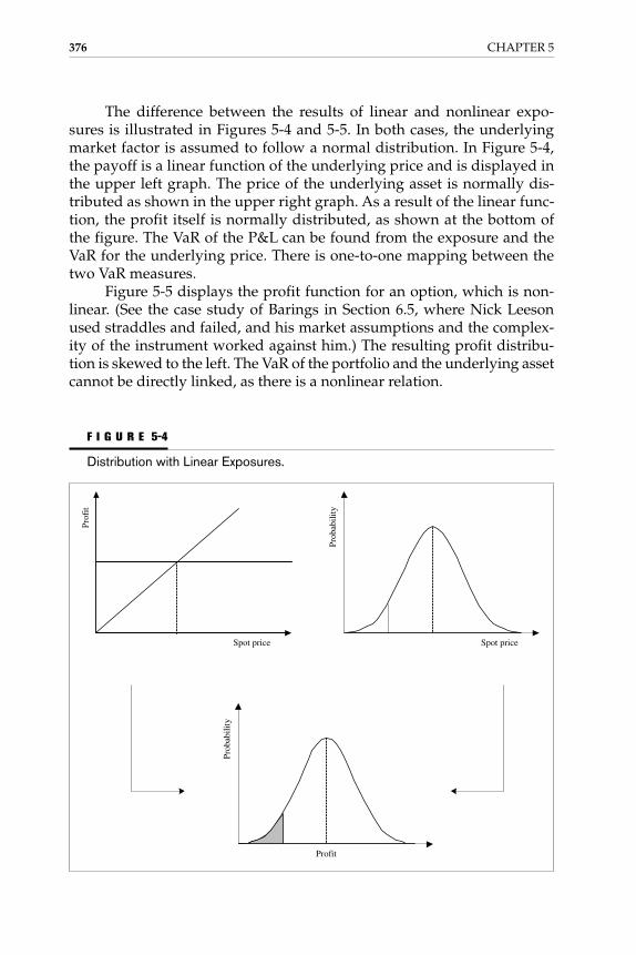
The difference between the results of linear and nonlinear expo-sures is illustrated in Figures 5-4 and 5-5. In both cases, the underlyingmarket factor is assumed to follow a normal distribution. In Figure 5-4,the payoff is a linear function of the underlying price and is displayed inthe upper left graph. The price of the underlying asset is normally dis-tributed as shown in the upper right graph. As a result of the linear func-tion, the profit itself is normally distributed, as shown at the bottom ofthe figure. The VaR of the P&L can be found from the exposure and theVaR for the underlying price. There is one-to-one mapping between thetwo VaR measures.

Figure 5-5 displays the profit function for an option, which is non-linear. (See the case study of Barings in Section 6.5, where Nick Leesonused straddles and failed, and his market assumptions and the complex-ity of the instrument worked against him.) The resulting profit distribu-tion is skewed to the left. The VaR of the portfolio and the underlying assetcannot be directly linked, as there is a nonlinear relation.

376 CHAPTER 5

Spot price Spot price

Profit

Prof

it

Prob

abili

ty

Prob

abili

ty

F I G U R E 5-4

Distribution with Linear Exposures.


5.6.2.3 Delta-Gamma MethodThe main drawback of the delta-normal method is that all risk parametersexcept the delta coefficient are lost. The elegance of the standardized ap-plication on different risk factors and among large portfolios is that it isgiven a simplification that strips away all nonlinear components. The Tay-lor expansion contains gamma and theta risks, which can be added to cap-ture the nonlinear risk components (the expansion can also include vegarisk to reflect exposures in volatility changes; however, this has beendropped in this example for simplicity).

V1 = V0 + δ(P1 − P0) + Γ(P1 − P0)2 (5.12)

and

V1 = V0 + δ(P1 − P0) + Γ(P1 − P0)2 − θt (5.13)1�2

1�2


Spot price Spot price

Profit

Prof

it

Prob

abili

ty

Prob

abili

ty

F I G U R E 5-5

Distribution with Nonlinear Exposures.


where t is the length of the forecast horizon and δ, Γ, and θ are net valuesfor the total portfolio including options, which are all written on the sameunderlying instrument18 and are defined by:

Γ = V(P,S,τ)|P0 (5.14)

θ = V(P,S,τ)|τ0 (5.15)

Figure 5-6 shows the delta, delta and gamma, and full valuation foran option. As can be seen, the delta-gamma-theta approximation almostperfectly duplicates the full valuation case.

Using a delta-normal approach, VaR is written as:

VaR1 = |δ|(ασS) (5.16)

where α is a function of the selected confidence level.

∂�∂τ

∂2

�∂R2

378 CHAPTER 5

0.08

0.07

0.06

0.05

0.04

0.03

0.02

0.01

0

– 0.01

0.5 0.6 0.7 0.8 0.9 1.0 1.1 1.2 1.3

Full valuation

Delta-gamma approach

Delta-normal approach

F I G U R E 5-6

Delta-Gamma-Theta Approximation versus Full and Delta Approximation.


Using higher-order terms, VaR can be written as:

VaR1 = |δ|(ασS) − Γ(ασS)2 − |θ| |Sdσ| (5.17)

A negative Γ represents a net short position in options, which resultsin an add-on for the second term; otherwise the second term will decreasethe total VaR. The third term θ represents an add-on to VaR due to expo-sures in changes in the time to maturity. Given a net long position with anegative θ, dσ leads to a positive change (increase) in time at the α confi-dence level; otherwise, for a net short position with a positive θ, dσ leadsto a decreasing volatility at the α confidence level.

Moving away from linearity, the calculation of the distribution ofchanges in the portfolio value V becomes complex and cannot be directlylinked to the VaR of the underlying position or portfolio.

The delta-gamma approach can be applied to many sources of risk.One approach to finding the portfolio VaR is the simulation of the move-ments in the market prices dS. Using a simulation technique, a large real-ization can be derived from the distribution

dS ≈ N(0,Σ) (5.18)

where Σ represents the covariance matrix of changes in prices.The delta-gamma approach is unfortunately not very practical be-

cause, as it requires many sources of risk, the required amount of data in-creases geometrically. For example, for a portfolio with N = 100, 100estimates are required of δ, 5050 estimates for the covariance matrix Σ, andan additional 5050 estimates for the matrix Γ, including the second deriv-atives of each position within the portfolio with respect to each source ofrisk. Thus, for such a portfolio, a full Monte Carlo simulation approachprovides a more efficient and effective VaR measurement.

5.6.2.4 Comparison of Delta Versus Full ValuationEach of the discussed methods is best adapted to a different application:

• The delta-normal approach fits best with large portfolios whereoptionality is not a dominant component.

• The delta-gamma approach fits best with portfolios with limitedexposures to risk factors and with a dominant optionalitycomponent, as it provides superior precision with reasonablecomputational requirements.

• The full valuation or Monte Carlo simulation approaches fit bestwith portfolios with substantial components of optionality andexposures to several risk factors.

1�2



The discussion of the linear/nonlinear component has direct impli-cations for the selection of the time horizon. With linear approaches, VaRcan be easily adjusted to other periods by simply scaling a square root oftime factor. These time horizon adjustments are based on the assumptionthat the position is constant and that all (daily) returns are independentand identically distributed. These time horizon adjustments are not appli-cable for positions with substantial components of optionality. As deriva-tive instruments can be replicated by dynamically changing positions inthe underlying assets, the risk of the derivative instruments can be dra-matically different from the scaled measure of daily risk. Thus, time hori-zon adjustments of daily volatility to longer time horizons using thesquare root of the time scaling factor are valid only when positions areconstant and when optionality in the portfolio is negligible. The full valu-ation or Monte Carlo simulation approach must be applied for portfoliosor positions with substantial optionality components over the requiredtime horizon, instead of scaling a daily VaR measure.

5.6.3 Historical Simulation Method

The historical simulation method can be viewed as a straightforward im-plementation of the full valuation method. By going back in time—say, for250 days—and applying current weights to a time series of historical assetreturns, the history of a hypothetical portfolio using the current position isgenerated.

Rp,τ = �N

i = 1

wi,t ⋅ Ri,τ τ = 1, . . . , t (5.19)

The weights wt are kept at their current values, not the historical val-ues. The full valuation requires a set of complete prices, such as yieldcurves. Hypothetical future prices for scenario τ are derived from apply-ing historical price movements to the current level of prices:

P*i,τ = P*i,0 + ∆Pi,τ i = 1, . . . , N (5.20)

A new portfolio value P*p,τ is calculated from the full set of hypotheticalprices, including nonlinear optionality components. In order to capturevega risks, the set of prices used can incorporate implied volatility measuresto accommodate the option’s price change relative to changes in volatility.This generates the hypothetical return corresponding to observation τ:

Rp,τ = (5.21)P*p,τ − Pp,0�

Pp,0

380 CHAPTER 5


VaR is then calculated from the entire distribution of hypothetical re-turns. This method is relatively straightforward to implement if historicaldata has been collected over a certain time period. The choice of the lengthof the sample period reflects the trade-off between longer and shortersample sizes. Longer time periods increase the accuracy of the estimates;in contrast, the estimate based on a shorter time frame might be irrelevantdue to missing important changes in the underlying data caused by short-term structural changes.

This method considers the selection of time horizon for measuringVaR as the returns are calculated simply over intervals that correspond tothe length of the VaR time horizon. For example, to calculate a monthlyVaR, historical monthly portfolio returns are calculated over the last fiveyears.

Being based on actual prices, this method is independent regardingnonlinearities and nonnormal distribution and thus captures gamma,vega risk, and correlations. The full valuation is based in its simplestform on historical data. The approach does not depend on assumptionsand conditions about valuation models or the underlying stochasticstructure of the instruments. It considers fat tails and is not prone tomodel risk.

However, the historical simulation method is subject to a number ofcriticisms. The most critical assumption of the historical simulationmethod is that the past foretells the future. Another issue is that risk con-tains significant and predictable time variation. The historical simulationapproach tends to overestimate the meaningfulness of historical data forthe future and to miss situations with temporarily elevated volatilities orstructural changes.

The quality of VaR measures calculated with the historical simula-tion method is linked to the length of the historical period, with the sameadvantages and disadvantages discussed earlier. Another debated issue isthe moving average estimation of variances. The historical simulationmethod allocates the same weight to all observations over the length of thetime horizon. As the observation period can include data from structuralchanges, and short-term elevated volatilities, the measure of risk canchange significantly after an old observation is excluded from the timewindow.

The last critical issue relates to large portfolios with complex instru-ments, which require extensive databases and computational power. Asimplification used in practice is the bucketing approach, where cashflows are allocated into time bands, such as interest rate payoffs, divi-dends, etc. This increases the speed of computation and is accepted andadopted by the regulators. If the bucketing approach is used with toomany simplifications, the benefits of full valuation can be lost due to low-ered accuracy and precision of the VaR information received.



5.6.4 Stress Testing

Stress testing is completely different from historical or Monte Carlo simu-lation. Stress tests, sometimes called scenario analyses, are designed to esti-mate potential economic losses in abnormal markets to examine the effecton key financial variables on the portfolio. Historical analysis of marketsshows that returns have fat tails, where extreme market moves (i.e., be-yond 99 percent confidence) occur far more frequently than a normal dis-tribution would suggest. Although risk management as a practice hasimproved considerably, events such as natural disasters, wars, and politi-cal coups still lie beyond statistical forecasting. For instance, a scenariowhere the yield curve moves up by 100 basis points over a month, orwhere a currency is suddently devalued by 20 percent, can be specified.

Regular stress testing is increasingly viewed as indispensable by riskmanagers and regulators. Stress tests should enhance transparency by ex-ploring a range of potential low-probability events when VaR bands aredramatically exceeded. Stress testing combined with VaR gives a morecomprehensive picture of risk. Such scenarios are well known within thetraditional asset liability management (ALM) approach.

The usefulness of such an approach depends on whether such sce-narios adequately represent typical market moves. Stress testing shouldanswer two central questions:

1. How much is the loss if a stress scenario occurs, e.g., if the U.S.equity market crashes by 20 percent?

2. What event or risk factor could cause an institution to lose morethan a predefined threshold amount, e.g., $1 million?

The first issue is commonly covered by a top-down approach forstress testing. Senior management or regulators want to be informedabout how much the firm may lose in a major equity market crash. Thesecond issue is usually raised in a bottom-up environment, such as at thebook or business level. After scenarios are collected from individual risktakers, their potential losses can be measured and aggregated over the dif-ferent exposures of the risk takers. For example, a stress scenario of de-preciation of Euros vs. U.S. dollars might be ruled unimportant due togenerally offsetting sensitivities (or nonmaterial reported sensitivities),while a scenario of widening credit spreads (e.g., lower ratings) could be identified as relevant. This approach could therefore be viewed as abottom-up search for relevant stress scenarios.

5.6.4.1 How to Use Stress TestsThe key issue with stress tests is how to create and use them. To be mean-ingful, stress tests should tie back into the decision-making process. Corporate-level stress test results should be discussed in a regular forum

382 CHAPTER 5


by risk monitors, senior management, and risk takers. Just as for VaR lim-its, companies should have a set of stress loss limits categorized by risktype and risk-taking unit.

Stress testing should be performed at multiple levels of the micro,macro, and strategic risk pyramid at different frequencies. At a seniormanagement level, stress results should guide the firm’s appetite for ag-gregate risk taking and influence the internal capital allocation process. Atthe book level, stress tests may trigger discussions on how best to unwindor hedge a position.

5.6.4.2 Development of Stress Test ParametersThe goal of stress testing is to uncover potential concentration risks andmake them more transparent. Good stress tests should therefore:

• Be relevant to current exposures. A concentrated portfolio withlarge risks may incur substantial losses from relatively smallmovements in certain risk factors.

• Consider changes in all relevant risk factors. Stress scenarios shouldconsider all potential changes in a complete set of risk factors. Astress scenario in isolation does not reflect reality, as risk factorsdon’t move in isolation (especially when they are extreme).

• Examine potential structural changes. A key question indeveloping a stress scenario is whether current risk parameterswill hold or break down under extreme conditions. It is key toknow if observed correlations hold or increase, or to what extenta structural change (i.e., decoupling of risk factors) could occur.For example, during large equity shocks (e.g., the 1987 crash andthe 1997 and 1998 sell-offs), a flight to safety often results in areversal of the normally highly positive correlation betweenstocks and government bonds: as stocks plummet, bonds risebecause investors move into safer and more liquid assets. In themarket turmoil of September 1998, LTCM experienced thisproblem when credit spreads widened and interest rates fell dueto a flight to safety.

• Consider market illiquidity. Stressed markets are oftencharacterized by material loss of liquidity. Liquidity can beviewed from two perspectives: the ability to trade positionswithout moving the prices and the ability to fund positions. Forexample, Brazilian bond traders reported that bid-ask spreadswere so wide during the October 1997 liquidity crisis that it wasunclear whether the local yield curve was upward or downwardsloping. As prices in the marketplace cease to exist, it becomesimpossible to mark positions to market. The threat of liquidityrisk motivated the recapitalization of LTCM by a consortium of



14 commercial and investment banks in September 1998. In astatement to the U.S. House of Representatives, Federal ReserveChairman Alan Greenspan stated that “the consequences of afire sale triggered by cross-default clauses, should LTCM fail onsome of its obligations, risked a severe drying up of marketliquidity.19

• Consider the interplay of market and credit risk. Stressed marketsoften give rise to counterparty exposures that may be much moresignificant than pure market impacts. While market rates andcreditworthiness are unrelated for small market moves, largemarket movements could precipitate credit events, and viceversa. A market-neutral risk arbitrage book would consist of aseries of long and short positions, which hedges out market riskbut is exposed to firm-specific risk. A trading strategy thateliminates broad market risk (equity, interest rates, foreignexchanges, or commodities) leaves only residual risk. Forexample, a hedge fund manager can hedge the market risk of aU.S. stock portfolio by shorting S&P 500 Index futures, leavingonly firm-specific residual risk.

5.6.4.3 Forecasting Time FrameThe forecast time horizon for the stress scenario should reflect the institu-tion’s typical holding period. Banks, brokers, and hedge funds tend tolook at one-day to one-week worst-case forecasts, while longer-term in-vestors, such as mutual and pension funds, may view a one-month tothree-month time frame as adequate. Corporations may use up to an an-nual horizon for strategic scenario analysis.

Steps for Stress TestingThere are three basic steps for stress testing:

1. Generate scenarios. The most challenging aspect of stress testingis generating credible worst-case forecasts that are relevant toportfolio positions. Scenarios should address both the magni-tude of movement of individual market variables and the inter-relationship of variables (i.e., correlation or causality).

2. Revaluate the portfolio/positions. Revaluing a portfolio or posi-tion involves marking to market all financial instruments undernew worst-case market rates. Stress test results are generallychanges in present value, not VaR.

3. Aggregate results. The results have to be aggregated to show ex-pected levels of mark-to-market losses or gains for each stressscenario and in which entity the losses or gains are concentrated.

384 CHAPTER 5


Creating Stress ScenariosThere are a variety of approaches to generating stress tests, such as:

• The predictive scenario generation, in which a subset of stressedrisk factors is used with historical volatilities or correlations topredict the moves of all other market variables.

• A natural approach, in which scenarios are based on historicalperiods with extreme market conditions (see Table 5-10). Someinfamous events include the 1987 U.S. stock market crash, theExchange Rate Mechanism (ERM) crisis, the Fed rate hike in 1994,the 1995 Tequila crisis, the 1997 Asian crisis, the volatile marketsin 1998, and the 1999 Brazil devaluation. In this approach, data iscaptured from relevant historical stress periods and a portfolio isvalued with historical simulation to measure potential losses.RiskMetrics research has assembled a representative globalmodel portfolio consisting of 60 percent equities and 40 percentfixed-income instruments to identify pertinent time periods forhistorical stress tests. Both one-day and five-day portfolio returnswere used to identify extreme loss periods.

How does the severity of loss depend on global volatility? Figure5-7 shows the volatility of the Nasdaq index for a period that includes threeof the historical scenario dates. Obvious patterns can be seen during thetime of the Gulf War, the Asian crisis, and the TMT crisis in March/April2000.


T A B L E 5-10

Major Loss Events of the Past 20 Years

One-Day Five-DayDate Return (%) Date Return (%)

Black Monday 10/19/87 −2.20 10/20/87 −5.9

Gulf War 8/3/90 −0.90 8/27/98 −3.8

Mexican peso fallout* 1/23/95 −1.00 1/23/95 −2.7

Asian crisis 10/27/97 −1.90 8/7/90 −3.6

Russian currency devaluations 8/27/98 −3.80 10/27/97 −2.6

SOURCE: RiskMetrics Group, Risk Management: A Practical Guide, New York: RiskMetrics Group, 1999, p. 28, reproductionwith permission of RiskMetrics Group, Inc.

*The Mexican peso was actually devalued at the end of 1994. On January 23, 1995, the peso lost 6 percent and severalEastern European markets incurred losses of around 5 to 10 percent.


5.6.4.4 Evolution of Shocks from VolatilityThe severity of portfolio losses appears to be related to the level of volatil-ity in the world. For example, the Mexican peso fallout, which occurredduring a period of relative market calm when the RiskMetrics VolatilityIndex (RMVI) was at an average level of approximately 100, only resultedin a one-day return of −1 percent, while the Asian crisis and Russian de-valuation, which occurred while the RMVI was significantly above 100,resulted in more severe portfolio losses of 1.9 percent and 3.8 percent (seeFigure 5-8). This suggests that it make no sense to run the same staticstress tests in all market regimes—more volatile markets require more se-vere stress tests. To make stress scenarios more responsive to market con-ditions, the RMVI can be used as a dynamic scaling factor for stressscenarios. The RMVI is a benchmark portfolio that measures globalvolatility and is composed of equity, fixed income, and foreign exchangemarkets in 28 countries, as well as three major commodity markets. Ob-serving the daily returns of these 87 markets, RiskMetrics calculates a totalvolatility across all countries and asset classes and compares it to a histor-ical average. For more information, see Christopher Finger, RMG VolatilityIndex: Technical Document, New York: RiskMetrics Group, 1998.

386 CHAPTER 5

–15%

–10%

–5%

0%

5%

10%

15%

8/1/

1989

Nas

daq

inde

x re

turn

s

11/1

/198

92/

1/19

905/

1/19

908/

1/19

9011

/1/1

990

2/1/

1991

5/1/

1991

8/1/

1991

11/1

/199

12/

1/19

925/

1/19

928/

1/19

9211

/1/1

992

2/1/

1993

5/1/

1993

8/1/

1993

11/1

/199

32/

1/19

945/

1/19

948/

1/19

9411

/1/1

994

2/1/

1995

5/1/

1995

8/1/

1995

11/1

/199

52/

1/19

965/

1/19

968/

1/19

9611

/1/1

996

2/1/

1997

5/1/

1997

8/1/

1997

11/1

/199

72/

1/19

985/

1/19

988/

1/19

9811

/1/1

998

2/1/

1999

5/1/

1999

8/1/

1999

11/1

/199

92/

1/20

005/

1/20

008/

1/20

0011

/1/2

000

2/1/

2001

5/1/

2001

8/1/

2001

F I G U R E 5-7

Nasdaq Index Returns from July 1989 to July 2001. Data source: Bloomberg Professional.


5.6.4.5 Applying Shocks to Market Factors or CorrelationsA second approach to generating stress tests is to apply large shocks to ei-ther market factors or volatilities and correlations. This method can pro-vide a good measure of the sensitivity to risk factors and can therefore beuseful in identifying trouble spots in a portfolio.

It is straightforward to alter a market rate (e.g., to lower the S&P 500by 10 percent) or many market rates (e.g., to lower all points on the U.S.government yield curve by 50 basis points), but the real challenge is to de-termine which market rates to shock and by how much. In general, thesedecisions will be based on historical moves, intuition, and the characteris-tics of the portfolio itself.

5.6.4.6 Applying Shocks to Volatilities and CorrelationsVaR estimates can be stressed by applying shocks to volatilities or correla-tions. While volatilities can be adjusted up and down like market rates,special care must be taken with correlation matrices because nonsensicalcorrelation structures can often be created from the interrelationship be-tween factors. These correlation structures can, in turn, result in nonsensi-cal (imaginary) VaRs.


Mexican pesocrisis Asian crisis Russian

devaluations

F I G U R E 5-8

Riskmetrics RMVI Methodology Applied to the Mexican Peso and U.S. Dollar fromDecember 1995 to March 1999. (Source: RiskMetrics Group, Risk Management:A Practical Guide, New York: RiskMetrics Group, 1999, 28. Copyright © 1999 byRiskMetrics Group, all rights reserved. Reproduction with permission of RiskMet-rics Group, LLC.)


For example, consider a three-party government. If party A and partyB always vote on opposite sides of every issue (correlation of −1), it is im-possible for party C to be positively correlated with both A and B. RiskMet-rics has published a methodology to adjust correlations in a mathematicallyconsistent fashion. The general idea is to mix an average correlation terminto a prespecified group of assets and then to adjust all diagonal terms.This methodology is implemented in CreditManager, where it can be usedto change the average correlation among industries and countries.

5.6.4.7 Anticipatory ScenariosIn generating an anticipatory scenario, a risk manager must determine theevent of interest (e.g., flight to quality within Asian markets, stock marketcrash), the severity of the event (e.g., from once a year to once a decade),and the effects of such an event on the global market. For the third deter-mination, it is essential to move all market rates in a consistent fashion.For example, in a flight to quality, not only will government-corporatespreads widen, but equity prices will fall.

The next step in the stress test is to revalue the portfolio under thisscenario and to analyze sensitivities and summarize the results.

5.6.4.8 Applying Portfolio-Specific Stress TestsAnother stress testing approach searches for stress scenarios by analyzingthe vulnerabilities of the specific portfolio in question. One way to discernthe vulnerabilities is by conducting a historical or Monte Carlo simulationon a portfolio and searching for all scenarios that could cause a loss ex-ceeding a defined threshold amount. Instead of specifying the scenarioand calculating potential losses, as in the three approaches described pre-viously, we specify what constitutes a severe loss and search for scenarios.

5.6.5 Summary of Stress Tests

Most models make assumptions that don’t hold up in abnormal markets.Stress tests are therefore essential for a comprehensive risk picture andshould be an integral component of risk analysis and communication.

As with VaR analysis, stress testing must be done at different levels ofthe organization. The organizational hierarchy for stress testing is evenmore important than for VaR reporting. At the desk level, traders are inter-ested in stressing individual positions and specific risk factors. On a corpo-rate level, senior management is concerned about macro stress scenariosthat could pose a threat to firmwide operations. The process of generatingand discussing stress scenarios is a collective exercise in risk analysis.Stress tests are an opportunity to consider scenarios that most view as un-likely, but that are possible. Make stress tests workable, realistic, andtimely. Rather than stress-testing everything, focus on relevant position-

388 CHAPTER 5


specific stresses. It is important for stress tests to tie into the decision-making process: stress test results should guide corporate risk appetite de-cisions, impact limits, and be a judgmental factor in capital allocation.

Stress testing can be viewed from two perspectives: what would bethe potential losses if certain events occurred, or what stress events couldlead to losses of a certain magnitude? There are four major approaches forgenerating stress scenarios. The first uses historical scenarios and the sec-ond shocks market rates to examine portfolio sensitivities and concentra-tions. The third approach considers hypothetical future scenarios basedon current market conditions. The fourth approach searches for stress sce-narios by analyzing portfolio vulnerabilities.

5.7 PORTFOLIO RISK

As discussed earlier, portfolio risk is not new to the investment industry.Traders and merchants realized early that diversification reduces the riskof loss. In 1959, Harry Markowitz developed an analytical framework forportfolio analysis and looking at return and risk. The concept of portfoliorisk is not new. In order to gain better insight, the following sections focuson the concept of VaR in the portfolio context. VaR is applied systemati-cally to many sources of risk in the investment industry. We will mainlyapply a delta-normal approach, as this approach is a direct extension oftraditional portfolio risk analysis and is based on variances and covari-ances, well known from Markowitz and others.

VaR measures portfolio risk and, through decomposition in incre-mental VaR components, enables identification of the asset contributingthe most to the overall portfolio risk. A drawback of the linear VaR mod-els (based on the delta-normal approach) is that the size of the covariancematrix increases geometrically with the number of assets. Alternative ap-proaches to reduce the size of the covariance matrix involve using diago-nal and factor models.

5.7.1 Portfolio VaR

A portfolio p can be characterized by positions on a certain number of riskfactors. Once the structure of the decomposition is defined, the portfolioreturn is a linear combination of the returns on underlying assets, wherethe weights wi are given by the relative dollar amounts invested at the be-ginning of the period. Therefore, the VaR of a portfolio can be recon-structed from a combination of the risks of underlying securities.

The portfolio’s return from t to t + 1 is defined as:

rp,t + 1 = �N

i = 1

wi,t ⋅ ri,t + 1 (5.22)



where the weights wi,t are measured at the beginning of the observationperiod and sum to unity of 1 (100 percent). In matrix notation, the sameportfolio return can be defined as:

rp = [w1, w2, . . . , wN]� � = w′r (5.23)

where w′ represents the transposed vector (i.e., horizontal) of weights andr is the vertical vector containing individual asset returns (r1, r2, . . . , rN).

The expected value E(X) or the mean can be estimated as the weightedsum of all possible values, each weighted by its probability of occurence:

E(X) = �N

i − 1

pi ⋅ xi (5.24)

By extension of Equation (5.24), the portfolio’s expected return is de-fined as:

E(rp) = µp = �N

i − 1

wi ⋅ µi

and the portfolio’s variance is:

σ2p = �

N

i = 1

w12σ1

2 + �N

i = 1�

N

j = 1

wiwjσij

= �N

i = 1

w12σ1

2 + 2 �N

i = 1�

N

j < 1

wiwjσij (5.25)

The variance includes the risk of the individual positions and all thecross-products, reflected in N(N − 1)/2 different covariances.

With an increasing number of assets, it becomes difficult to generateand manage all the different covariances on an equation basis. In matrixnotation, the variance is written as:

σ2p = [w1, w2, . . . , wN]� � � � (5.26)

Defining cov as the covariance matrix, the portfolio variance can bewritten more compactly as:

w1

w2

wN

σ1,N

�

σN,N

. . .

. . .

σ1,3

σN,1

σ1,2

σN,1

σ1,1

�

σN,1

r1

r2

�

rN

390 CHAPTER 5


σ2p = w′ cov w (5.27)

Using a normal distribution, the VaR measure is then ασp times theinitial investment. Lower portfolio risk can be achieved through low cor-relations or a large number of assets. To see the effect of N, assume that allassets have the same risk, that all correlations are the same, and that equalweight is put on each asset. Figure 5-9 shows how portfolio risk decreaseswith the number of assets.

Start with the risk of one security, which is assumed to be 12 percent.When p is equal to 0, the risk of a 10-asset portfolio drops to 3.8 percent; in-creasing N to 100 drops the risk even further to 1.2 percent. Risk tends asymptotically to 0. More generally, portfolio risk is:

σp = σ + �1 −�ρ (5.28)

So, when p = 0.5, risk decreases rapidly from 12 percent to 8.9 per-cent as N goes to 10, but then converges much more slowly toward itsminimum value of 8.5 percent. Correlations are essential in loweringportfolio risk.

1�N

1�N


0

2

4

6

8

10

12

1 10 100 1000

Correlation = 0.5

Correlation = 0.0

Number of securities in portfolio

Ris

k (%

)

F I G U R E 5-9

Number of Securities in Portfolio and Impact on Correlation (Diversification).


Covariances can be estimated from sample data as:

σ̂ij = �T

t = 1

(xt,i − µ̂i)(xt,j − µ̂i) (5.29)

The covariance is a measure of the extent to which two variablesmove linearly together. If two variables are independent, their covarianceis equal to 0. A positive covariance means that the two variables tend tomove in the same direction; a negative covariance means that they tend tomove in opposite directions.

The magnitude of covariance, however, depends on the variances ofthe individual components and is not easily interpreted. The correlationcoefficient is a more convenient, scale-free measure of linear dependence:

ρ12 = (5.30)

The correlation coefficient ρ always lies between −1 and +1. When ρis equal to unity, the two variables are said to be perfectly correlated.When ρ is 0, the variables are uncorrelated.

Correlations help to diversify portfolio risk. With two assets, the di-versified portfolio variance is:

σ2p = w1

2σ 12 + w2

2σ22 + 2w1w2σ1ρ1,2σ2 (5.31)

The portfolio risk must be lower than individual risk. When the corre-lation is exactly unity, Equation (5.31) reduces the variance of the portfolio tothe weighted variance of the underlying positions, since the portfolio weightssum to unity. Generally, the undiversified VaR is the sum of individual VaRmeasures. Diversification into perfectly correlated assets does not pay.

So far, nothing has been said about the distribution of the portfolio re-turn. Ultimately, we would like to translate the portfolio variance into a VaRmeasure. To do so, we need to know the distribution of the portfolio return.In the delta-normal model, all individual security returns are assumed to benormally distributed. This is particularly convenient since the portfolio, alinear combination of normal random variables, is then also normally dis-tributed. At a given confidence level, the portfolio VaR is value at risk = ασp.

5.7.2 Incremental VaR

An important aspect of calculating VaR is to understand which asset, orcombination of assets, contributes most to risk. Armed with this informa-tion, users can alter positions to modify their VaR most efficiently.

σ1,2�σ1σ2

1�T − 1

392 CHAPTER 5


For this purpose, individual VaRs are not sufficient. Volatility meas-ures the uncertainty in the return of an asset taken in isolation. When thisasset belongs to a portfolio, however, what matters is the contribution toportfolio risk.

Suppose now that an existing portfolio is made up of N-1 securities,numbered as j = 1, . . . ,N-1. A new portfolio is obtained by adding one se-curity, called i. The marginal contribution to risk from security i is mea-sured by differentiating Equation (5.25) with respect to wi.

= 2wiσi2 + 2 �

N

j = 1,j ≠ i

wjσi, j

= 2 cov �ri, wiri + �N

j ≠ i

wjrj� = 2 cov (ri, rj) (5.32)

We note that ∂σ2p/∂wi = 2σp∂σp/∂wi. The sensitivity of the relative

change in portfolio volatility to a change in the weight is then:

= = βi (5.33)

Therefore, β measures the contribution of one security to total port-folio risk. This is also called the systematic risk of security i vis-à-vis port-folio p. Using matrix notation, β is:

β = (5.34)

Beta risk is the basis for the capital asset pricing model (CAPM), de-veloped by Sharpe (1964). According to the CAPM, well-diversified in-vestors want to be compensated for the systematic risk of securities only.In other words, the risk premium on all assets should depend on beta only.Whether this is an appropriate description of capital markets has been thesubject of much of finance research over the last 20 years. Even though thisproposition is much debated, the fact remains that systematic risk is a use-ful statistical measure of portfolio risk.

The measure of β is particularly useful for decomposing a portfolio’sVaR into sources of risk. We can expand the portfolio variance into:

σ2p = w1�w1σ1

2 + �N

j = 1, j ≠ 1

wiσ1,j�+ w2�w2σ2

2 + �N

j = 1, j ≠ 2

wiσ2,j�+ ⋅⋅⋅ (5.35)

cov w�w′ cov w

cov (ri, rj)��

σ2p

∂σp�σp∂wi

∂σ2p

�∂wi



This is also:

σ 2p = w1 cov (r1, rp) + w2 cov (r2, rp) + ⋅⋅⋅

= w1(β1σ 2p) + w2(β2σ 2

p) + ⋅⋅⋅

= σ 2p��

N

i = 1

wiβi� (5.36)

which shows that the portfolio variance can be decomposed into a sum ofcomponents each due to asset i. Using a similar decomposition, VaR is then:

VaR = VaR ��N

i = 1

wiβi� = VaR1 + VaR2 + ⋅⋅⋅ (5.37)

Here we have decomposed the total VaR into incremental measures.This provides vital information, as risk should be viewed in relation to thetotal portfolio and not in isolation.

5.7.3 Alternative Covariance Matrix Approaches

So far, we have shown that correlations are essential driving forces behindportfolio risk. When the number of assets is large, however, the measure-ment of the covariance matrix becomes increasingly difficult. With 10 as-sets, for instance, we need to estimate 10 × 11/2 = 55 different variance andcovariance terms. With 100 assets, this number climbs to 5500. The num-ber of correlations increases geometrically with the number of assets. Forlarge portfolios, this causes real problems: the portfolio VaR may not bepositive, and correlations may be imprecisely estimated.

The following sections discuss the extent to which such problemscan affect VaR measures and propose some solutions. For many users,however, such problems may not be relevant because they have no controlover the measurement of inputs. Until such users encounter zero VaRmeasures, these sections can be safely skipped.

5.7.3.1 Zero VaR MeasuresThe VaR measure derives from the portfolio variance, expressed as:

σ 2p = w′ cov w (5.38)

In order to generate statistically useful measures, the cov has to bepositive definite. This is not always the case. The status of the cov can beverified under two conditions:

394 CHAPTER 5


1. The number of historical observations T must be greater thanthe number of assets N.

2. The return time series cannot be linearly correlated.

The first condition states that if a portfolio consists of 100 assets,there must be at least 100 historical observations to ensure that whateverportfolio is selected, the portfolio variance will be positive. The secondcondition rules out cases where an asset can be replicated exactly througha linear combination of other assets.

An example of a non-positive-definite matrix is obtained when twoassets are identical (thus ρ = 1). In this situation, a portfolio consisting of$1 on the first asset and −$1 on the second will have exactly zero risk.

In practice, this problem is more likely to occur with a large numberof assets that are highly correlated (such as currencies fixed to each other,zero coupon bonds, or ADRs and the original foreign stock). In addition,positions must be precisely matched with assets to yield zero risk. This ismost likely to occur if the weights have been optimized on the basis of thecovariance matrix itself. Such optimization is particularly dangerous be-cause it can create positions that are very large, yet that apparently offseteach other with little total risk.

If users notice that VaR measures appear abnormally low in relationto positions, they should check whether small changes in correlations leadto large changes in their VaRs.

5.7.3.2 Diagonal ModelA related problem is that as the number of assets increases, it is more likelythat some correlations will be erroneously measured. Some models canhelp to simplify this process by providing a simpler structure for the co-variance matrix. One such model is the diagonal model, originally pro-posed by Sharpe in the context of stock portfolios. This model is oftenreferred to as the CAPM, which is not correct. The diagonal (one-factor)model is only a simplification of the covariance matrix and says nothingabout the nature of expected returns, whose description through the rela-tionship to the market factor is the essence of the CAPM.

The assumption is that the common movement in all assets is due toone common factor only, the market. Formally, the model is:

ri = αi + βirm + εi E(εi) = 0 E(εirm) = 0

E(εi,εj) = 0 E(ε i2) = σ 2

ε,i

(5.39)

The return on asset i is driven by the market return R and an idio-syncratic term εi, which is not correlated with the market or across assets.As a result, the variance can be broken down as:



σ i2 = βi

2σ 2m + σ 2

ε,i (5.40)

The covariance between two assets is:

σ i2 = βiβjσ 2

m (5.41)

which is solely due to the common factor. The full covariance matrix is:

Cov = � �[β1 . . . βN]σ 2m� � (5.42)

Written in matrix notation, the covariance matrix is:

Cov = ββ′σ 2m + Dε (5.43)

As the matrix D is diagonal, the number of parameters is reducedfrom N × (N + 1)/2 to 2N + 1(N for the betas, N in D and one for 0 − m).With 100 assets, for instance, the number is reduced from 5500 to 201, aconsiderable improvement regarding equation complexity and calcula-tion time. Furthermore, the variance of large, well-diversified portfolios issimplified even further, reflecting only exposure to the common factor.The variance of the portfolio is:

VaR(rp) = VaR(w′r) = w′ cov w = (w′ββ′w)σ 2m + w′Dεw (5.44)

The second term consists of

�N

i = 1

wi2σ 2

ε,i

But this term becomes very small as the number of securities in the port-folio increases. For instance, if all the residual variances are identical andhave equal weights, this second term is

��N

i = 1

(1/N)2�σ2ε,i

which converges to 0 as N increases. Therefore, the variance of the portfo-lio converges to:

VaR(rp) → (w′ββ′w)σ2m (5.45)

which depends on one factor only. This approximation is particularly use-ful when assessing the VaR of a portfolio consisting of many stocks. It has

0�

σ2ε,N

. . .

. . .

σ2ε,i

�

0

β1

�

βN

396 CHAPTER 5


been adopted by the Basel Committee to reflect the market risk of well-diversified portfolios.

The actual correlations are all positive, as are those under the diago-nal model. Although the diagonal model matrix resembles the original co-variance matrix, the approximation is not perfect. The diagonal modelmeasures risk in relation to the market, and thus the correlation is drivenby exposure to the market and is different (usually lower) than the true cor-relation. This is because the market is the only source of common variation.Whether this model produces acceptable approximations depends on thepurpose at hand. Despite the drawback of limitation in the explanatorypower of the model given only one source of common variation, there is noquestion that the diagonal model provides a considerable simplification.

5.7.3.3 Factor ModelsIf a one-factor model is not sufficient, better precision and more statisticalstability can be obtained with multiple-factor models. Equation (5.46) canbe generalized to K factors:

ri = αi + βi ,1ri + . . . + βi,krk + εi (5.46)

where r1, . . . , rk are factors independent of each other. In the previousthree-stock example, the covariance matrix model can be improved with asecond factor, such as the performance of the transportation industry, thatwould pick up the higher correlation between two stocks. With multiplefactors, the covariance matrix acquires a richer structure:

Cov = β1β′1σ 21 + . . . + βkβ′kσk

2 + Dε (5.47)

The total number of parameters is (K + N × K + N), which may still beconsiderably less than for the full model. With 100 assets and five factors,for instance, the number is reduced from 5500 to 605, which is no minordecrease.

Factor models are also important because they can help us decide onthe number of VaR building blocks for each market. Consider, for instance,a government bond market that displays a continuum of maturities rang-ing from one day to 30 years. The question is, how many VaR buildingblocks do we need to represent this market adequately?

To illustrate, consider an equity market—say, the Swiss equity mar-ket—and calculate the principal components for the returns of the securitiesof the Swiss Mark Index (SMI). The next step is to regress in an orthogonalspace the principal components against the factors, which can best explainthe principal components (variation of returns). The principal componentsare by construction orthogonal. The factors contain multicolinearity, and,through an additional condition during the Lagrange optimization—intro-duction of unit vectors with components summing to 1—a series of vectors



can be estimated that provide the best explanation of diagonal terms (thecommon factors, e.g., the market) and are orthogonal to each other. The re-sults are presented in Table 5-11. Principal component 1 can be best explainedby the Euro Currency Swiss Franc 1 Month factor, explaining 42.28 percent ofthe principal component. With an R2 of 15.03, the second principle compo-nent was acceptably explained by the EFFAS Switzerland Government BondIndex, but the result was already considerably weaker, as reflected in the cor-responding statistics. The following factors do not fully help us understandthe return variation. However, the overall impact of such a multifactor modelis to help us understand more than we would using solely a diagonal model,as it breaks down the common factor into several multiple factors.

Table 5-12 illustrates the relationship between the principal compo-nents and the factors. The factor loadings of the factors to the principal com-

398 CHAPTER 5

T A B L E 5-11

Principal Component and Factor Combination

Principalcomponent Factor Name R2 C(p) F Value

1 ECSWF1M Euro Currency Swiss Franc 1 Month 0.4228 1117.36 104.73

2 DEFSWAL EFFAS Switzerland Government 0.1503 47.383 26.69

3 ECWGM7D Euro Currency German Mark 7 Days 0.0353 −23.544 5.23

4 SAPCOMP Standard & Poor’s 500 Composite 0.0443 −10.774 6.63

5 ECWGM3M Euro Currency German Mark 3 Months 0.06 3.5143 9.13

6 BDBRYLD EFFAS Germany Benchmark Bond 0.0382 −37.938 5.67

7 DEFJPG5 EFFAS Japan Government over 5 Years 0.0598 −14.104 9.1

8 FTSE100 FTSE100 Index 0.0479 48.0762 7.19

9 DEFUSG5 EFFAS U.S. Government over 5 Years 0.0362 −27.495 5.73

10 DEFBDAL EFFAS Germany Government 0.0758 4.0806 11.72

SOURCE: Reto R. Gallati, “Empirical Application of APT Multifactor-Models to the Swiss Equity Market,” Basic Report, Zurich: CreditSuisse Investment Research, September 1993.


399

T A B L E 5-12

Correlation of Principal Components to Factors from 08/08/1988 to 03/31/1993

PRIN1 PRIN2 PRIN3 PRIN4 PRIN5 PRIN6 PRIN7 PRIN8 PRIN9 PRIN10

ECSWF1M -0.60 0.11 0.09 0.06 0.01 −0.12 0.03 0.01 0.08 0.07

DEFSWAL 0.02 0.35 −0.16 0.02 −0.12 −0.05 −0.04 −0.09 0.24 0.09

ECWGM7D −0.01 0.01 -0.13 0.08 0.07 −0.08 0.12 −0.02 0.01 0.03

SAPCOMP 0.02 −0.01 0.06 -0.21 0.07 −0.07 −0.03 −0.10 −0.02 −0.09

ECWGM3M −0.02 −0.06 0.14 0.07 -0.14 0.05 0.02 0.08 −0.04 0.05

BDBRYLD 0.00 −0.04 0.01 0.10 −0.05 -0.12 −0.03 0.05 −0.10 −0.01

DEFJPG5 −0.01 0.04 0.02 0.09 0.01 −0.09 0.21 0.04 −0.03 −0.01

FTSE100 0.04 0.15 0.03 0.12 0.02 0.12 0.06 -0.19 0.05 −0.04

DEFUSG5 −0.02 −0.01 0.04 0.05 −0.08 0.08 0.14 −0.09 -0.18 −0.05

DEFBDAL 0.00 −0.01 −0.03 0.02 0.06 −0.05 0.06 −0.01 0.05 -0.24

SOURCE: Reto R. Gallati, “Empirical Application of APT Multifactor-Models to the Swiss Equity Market,” Basic Report, Zurich: Credit Suisse Investment Research, September 1993.


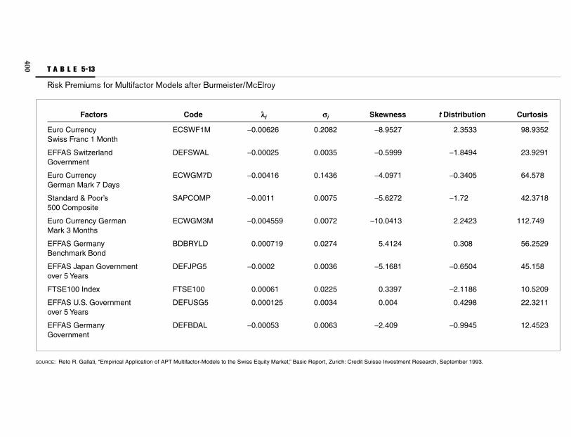
T A B L E 5-13

Risk Premiums for Multifactor Models after Burmeister/McElroy

Factors Code lj sj Skewness t Distribution Curtosis

Euro Currency ECSWF1M −0.00626 0.2082 −8.9527 2.3533 98.9352Swiss Franc 1 Month

EFFAS Switzerland DEFSWAL −0.00025 0.0035 −0.5999 −1.8494 23.9291Government

Euro Currency ECWGM7D −0.00416 0.1436 −4.0971 −0.3405 64.578German Mark 7 Days

Standard & Poor’s SAPCOMP −0.0011 0.0075 −5.6272 −1.72 42.3718500 Composite

Euro Currency German ECWGM3M −0.004559 0.0072 −10.0413 2.2423 112.749Mark 3 Months

EFFAS Germany BDBRYLD 0.000719 0.0274 5.4124 0.308 56.2529Benchmark Bond

EFFAS Japan Government DEFJPG5 −0.0002 0.0036 −5.1681 −0.6504 45.158over 5 Years

FTSE100 Index FTSE100 0.00061 0.0225 0.3397 −2.1186 10.5209

EFFAS U.S. Government DEFUSG5 0.000125 0.0034 0.004 0.4298 22.3211over 5 Years

EFFAS Germany DEFBDAL −0.00053 0.0063 −2.409 −0.9945 12.4523Government


400


401

T A B L E 5-14

Correlations of SMI Securities on Excess Returns

CSH UBS RUKP WI ZUR ALU CIG CIGN ROG NES NESN SR HOL

CSH 1.00

UBS 0.72 1.00

RUKP 0.56 0.59 1.00

WI 0.55 0.59 0.72 1.00

ZUR 0.55 0.63 0.74 0.82 1.00

ALU 0.52 0.53 0.48 0.53 0.49 1.00

CIG 0.45 0.52 0.59 0.62 0.64 0.63 1.00

CIGN 0.43 0.46 0.40 0.40 0.41 0.61 0.69 1.00

ROG 0.54 0.59 0.56 0.57 0.58 0.58 0.70 0.67 1.00

NES 0.43 0.45 0.55 0.55 0.57 0.47 0.62 0.35 0.57 1.00

NESN 0.31 0.34 0.06 0.14 0.12 0.31 0.12 0.48 0.36 0.05 1.00

SR 0.36 0.50 0.37 0.44 0.41 0.40 0.50 0.43 0.51 0.38 0.30 1.00

HOL 0.45 0.47 0.44 0.42 0.43 0.53 0.51 0.49 0.52 0.38 0.28 0.45 1.00



T A B L E 5-15

Factor Loadings According to Multifactor Calculations for SMI, Compiled 02/14/1992

SMI TS SMI Security ECSWF1M DEFSWAL ECWGM3M FTSE100 R2 R2 Adjusted

ALU Alusuisse-Lonza BS −1.85 0.63 −0.70 0.98 28.4% 26.9%

CIG Ciba-Geigy BS −1.97 0.46 −0.67 1.40 31.6% 30.2%

CIGN Ciba-Geigy RS −1.86 0.39 −0.83 1.01 29.0% 27.4%

CSH CSHolding BS −1.92 0.54 −0.58 0.73 34.4% 33.0%

HOL Holderbank BS −1.97 0.27 0.12 0.58 35.3% 33.9%

NES Nestlé BS −2.04 0.12 −0.31 0.72 36.9% 38.6%

NESN Nestlé RS −1.67 −0.0099 −0.68 0.71 26.8% 25.2%

ROG Roche DRC −1.97 0.42 −0.49 0.57 35.6% 34.2%

RUKP Schweizer Rück PC −2.00 0.54 −0.09 0.26 32.5% 31.1%

UBS UBS BS −1.96 0.48 −0.78 0.80 37.4% 36.1%

SR Swissair BS −1.82 0.42 0.68 1.48 28.7% 27.1%

WI Winterthur BS −1.96 0.74 0.12 0.45 33.2% 31.8%

ZUR Zurich BS −1.94 0.73 −0.36 0.31 33.5% 32.1%


402


ponents are highlighted with bold numbers. In this context, the sign is notrelevant, but the absolute correlation is important. The factor sensitivity re-flects the sign with a positive or a negative factor sensitivity (factor-beta βi).

Table 5-13 shows the risk premiums associated with this specific mul-tifactor model. The available test lambdas confirm the selection of five in-dices according to the risk premium from the two-stage least-squaresprocedure. On a basis of the results, the selected risk factors represent so-called priced factors, that is, factors that are rewarded with a risk premiumbecause they significantly influence the return on Swiss equities at the cor-responding level. From the test statistics of the principal component analy-sis, the risk premium, and other analysis, we can conclude that the followingfour factors are of sufficient significance for use in a multifactor APT model:

1. Euro Currency Swiss Franc 1 Month2. EFFAS Switzerland Government3. Euro Currency German Mark 3 Months4. FTSE100 Index

Table 5-14 displays the correlations between the securities, high-lighting the fact that for a small market like the Swiss equity market, thecorrelations between the securities can be small, offering good diversifica-tion but requiring different approaches in the return and risk evaluation,as the companies in the different sectors are exposed to different industryfactors and different company-specific factors.

Table 5-15 provides a summary of the results and contains the betasof the securities to the defined factors as analyzed and evaluated in theprevious statistical procedures.

This decomposition shows that the risk of an equity portfolio can beusefully summarized by its exposures to a limited number of factors. Dif-ferent types of models exist, such as models that keep the factors constantand allow tracking the same factors over time. Other models estimate thefactors on a regular basis and provide insight into the different factors asthey change over time and keep the overall explanatory power high.

5.8 PITFALLS IN THE APPLICATION AND INTERPRETATION OF VAR

Although VaR provides a line of defense against financial risks, it is nopanacea. Users must understand the limitations of VaR measures.

5.8.1 Event and Stability Risks

The main drawback of models based on historical data is that they assumethat the recent past is a good projection of future randomness. Even if the

403 CHAPTER 5


data has been perfectly fitted, there is no guarantee that the future will nothide nasty surprises that did not occur in the past.

Surprises can take two forms: either one-time events (such as a de-valuation or default) or structural changes (such as going from fixed tofloating exchange rates). Situations where historical patterns changeabruptly cause havoc with models based on historical data.

Stability risk can be addressed by stress testing (discussed in Section5.6.4), which aims at addressing the effect of drastic changes on portfoliorisk. To some extent, structural changes can also be captured by modelsthat allow risk to change through time or by volatility forecasts containedin options. An example of structural change is the 1994 devaluation of theMexican peso, which is further detailed in the following text.

In December 1994, the emerging market turned sour as Mexico de-valued the peso by 40 percent. The devaluation was widely viewed as hav-ing been bungled by the government, and led to a collapsing Mexican stockmarket. Investors who had poured money into the developing economiesof Latin America and Asia faced large losses as the Mexican devaluationled to a widespread decrease in emerging markets all over the world.

Figure 5-10 plots the peso-dollar exchange rate, which was fixedaround 3.45 pesos for most of 1994 and then jumped to 5.64 by mid-December. Figure 5-11 shows the distribution of the peso-dollar exchangerates for the same time frame. Apparently, the devaluation was widelyunanticipated, even with a ballooning current account deficit running at10 percent of Mexico’s GDP and a currency widely overvalued accordingto purchasing power parity.

This episode indicates that, especially when price controls are left inplace for long periods, VaR models based on historical data cannot cap-ture potential losses. These models must be augmented by an analysis ofeconomic fundamentals and stress testing. Interestingly, shortly after the

404 CHAPTER 5

0

1

2

3

4

5

6

7

8

9

1/4/

1993

3/4/

1993

5/4/

1993

7/4/

1993

9/4/

1993

11/4

/199

3

1/4/

1994

3/4/

1994

5/4/

1994

7/4/

1994

9/4/

1994

11/4

/199

4

1/4/

1995

3/4/

1995

5/4/

1995

7/4/

1995

9/4/

1995

11/4

/199

5

1/4/

1996

3/4/

1996

5/4/

1996

7/4/

1996

9/4/

1996

11/4

/199

6

Mex

ican

pes

o / U

.S. $

-20%

-15%

-10%

-5%

0%

5%

10%

15%

20%

25%

1/4/

1993

4/4/

1993

7/4/

1993

10/4

/199

3

1/4/

1994

4/4/

1994

7/4/

1994

10/4

/199

4

1/4/

1995

4/4/

1995

7/4/

1995

10/4

/199

5

1/4/

1996

4/4/

1996

7/4/

1996

10/4

/199

6

Dai

lyre

turn

s(l

n)

F I G U R E 5-10

Mexican Peso–U.S. Dollar Exchange Rate from 1993 to 1996. (Data source:Bloomberg Professional.)


devaluation, the Mexican government authorized the creation of currencyfutures on the peso. It was argued that the existence of forward-lookingprices for the peso would have provided market participants, as well asthe central bank, with an indication of market pressures. In any event, thisdisaster was not blamed on derivatives.

5.8.2 Transition Risk

Whenever there is a major change, a potential exists for errors. This ap-plies, for instance, to organizational changes, expansion into new marketsor products, implementation of a new system, or new regulations. Sinceexisting controls deal with existing risks, they may be less effective duringa transition.

Transition risk is difficult to deal with because it cannot be explicitlymodeled. The only safeguard is increased vigilance in times of transition.

5.8.3 Changing Holdings

A similar problem of instability occurs when trying to extrapolate dailyrisk to a longer horizon, which is of special concern to bank regulators.As we have seen in Secs. 3.6.2 and 3.7.5.2, the typical adjustment is by asquare root of time factor, assuming constant positions. However, theadjustment ignores the fact that the trading position might very wellchange over time in response to changing market conditions. There is nosimple way to assess the impact on the portfolio VaR, but it is likely thatprudent risk management systems will decrease risk relative to conven-tional VaR measures. For instance, the enforcement of loss limits willgradually decrease exposure as losses accumulate. This dynamic trading


–10%

0%

10%

20%

30%

40%

50%

60%

70%

80%

–0.200 –0.150 –0.100 –0.050 - 0.050 0.100 0.150 0.200

Normal distribution Current distribution

–10%

0%

10%

20%

30%

40%

50%

60%

70%

80%

–0.200 –0.150 –0.100 –0.050 - 0.050 0.100 0.150 0.200

Normal distribution Current distribution

F I G U R E 5-11

Distribution of Mexican Peso–U.S. Dollar Exchange Rates from 1993 to 1996, In-cluding (left) and Excluding (right) the Week Before and After the Devaluation.(Data source: Bloomberg Professional.)


pattern is similar to purchasing an option that has limited downside po-tential. It is also possible, however, as Barings has demonstrated, thattraders who lose money increase their bets in the hope of recouping theirlosses.

5.8.4 Problem Positions

Problem positions are in a category similar to transition. All the analyticalmethods underlying VaR assume that some data is available to measurerisks. However, for some securities, such as infrequently traded emerg-ing market stocks, private placements, or exotic currencies, meaningfulmarket-clearing prices may not exist.

Without adequate price information, risk cannot be assessed fromhistorical data (not to mention implied data). Yet, a position in these assetswill create the potential for losses that is difficult to quantify. In the ab-sence of good data, educated stress testing appears to be the only methodto assess risks.

5.8.5 Model Risks

Most risk management systems use past history as a guide to future risks.However, extrapolating from past data can be hazardous. This is why it isessential to beware of the pitfalls of model risks.

5.8.5.1 Functional Form RiskThis is the purest form of model risk. Valuation errors can arise if the spe-cific functional form selected for valuing a security is incorrect. The Black-Scholes model, for instance, relies on a rather restrictive set of assumptions(geometric Brownian motion, constant interest rates, and volatility). Forconventional stock options, departures from these assumptions generallyhave few consequences. However, there are situations where the model isinappropriate, such as for short-term interest rate options.

Model risk also becomes more dangerous as the instrument becomesmore complicated. Pricing CMOs requires heavy investments in the de-velopment of models, which may prove inaccurate under some marketconditions.

5.8.5.2 Parametric RiskAlso known as estimation risk, parameter risk stems from imprecision inthe measurement of parameters. Even in a perfectly stable environment,we do not observe the true expected returns and volatilities. Thus, somerandom errors are bound to happen just because of sampling variation.

As shown in the previous chapters, the effect of estimating risk couldbe formally assessed by replacing the sample estimates with values that

406 CHAPTER 5


are statistically equivalent. An alternative method consists of samplingover different intervals. If the risk measures appear to be sensitive to aparticular sample period, then estimation risk may be considerable.

Estimation risk increases with the number of estimated parameters.The more parameters that are estimated, the greater the chance that errorswill interact with each other and create a misleading picture of risk. Errorsin correlations are particularly dangerous when they are associated withlarge arbitrage positions. Parsimony breeds robustness.

The problem of estimation risk is often ignored in VaR analyses.Users should realize the fundamental trade-off between using more data,which leads to more precise estimates, and focusing on more recent data,which may be safer if risk changes over time.

Unfortunately, data may not be available for very long periods. Forinstance, only very limited histories are available for emerging markets orexotic currencies. This is all the more reason to remember that VaR num-bers are just estimates.

5.8.5.3 Data Mining RiskThis is among the most insidious forms of risk. It occurs when searchingvarious models and reporting only the one that gives positive results. Thisis particularly a problem with nonlinear models (such as neural networkor chaos models), which involve searching not only over parameter valuesbut also over different functional forms.

Data mining also consists of analyzing the data until some signifi-cant relationship is found. For instance, consider an investment managerwho tries to find calendar anomalies in stock returns. The manager triesto see whether stock returns systematically differ across months, weeks,days, and so on. So many different comparisons can be tried that, in 1case out of 20, we would expect to find significant results at the usual 5percent level. Of course, the results are significant only because of thesearch process, which discards nonsignificant models. Data mining riskmanifests itself in overly optimistic simulation results based on historicaldata. Often, results break down outside the sample period because theyare fallacious.

Data mining risks can be best addressed by running paper portfo-lios, where an objective observer records the decisions and checks how theinvestment process performs using actual data.

5.8.5.4 Survivorship RiskSurvivorship is an issue when an investment process only considers se-ries, markets, stocks, bonds, or contracts that are still in existence. Theproblem is that assets that have fared badly are not observed. Analysesbased on current data, therefore, tend to project an overly optimisticimage or display certain characteristics.



Survivorship effects are related to the “peso problem” in the foreignexchange market. Before the devaluation of 1982, the Mexican peso wasselling at a large discount in the forward market (the forward price of thepeso was well below the price for current delivery). This discount ration-ally anticipated a possible devaluation of the peso. An observer analyzingthe discount before 1982 would have concluded that the market was inef-ficient. The failure, however, was not that of the market, but rather of theobserver, who chose a sample period in which the data did not reflect anyprobability of a devaluation.

More generally, unusual events that have a low probability of occur-rence but that may have severe effects on prices, such as wars or national-izations, are not likely to be well represented in samples, and may betotally omitted from survivorship series. Unfortunately, these unusualevents are very difficult to capture with conventional risk models.

5.8.6 Strategic Risks

As explained in Chapter 1, VaR can help to measure and control financialrisk. However, it is impotent in the face of strategic risks that pose a chal-lenge to corporations. Strategic risks are those resulting from fundamentalshifts in the economy or political environment. One such example is thestory of Bankers Trust, which before 1994 was widely admired as a leaderin risk management, but became a victim of the backlash against deriva-tives. (See analysis of case studies in Section 6.1.) The derivatives markethas been subject to political and regulatory risks, which are part of themenagerie of strategic risks affecting corporations either at the firm or theindustry level.

Political risks arise from actions taken by policy makers that signifi-cantly affect the way an organization runs its business. These policies mayimpose limitations on the use of derivatives, thus negatively affecting theprofitability of many firms involved in that market. It is perhaps in re-sponse to these threats that the private sector has come up with initiativesto address the issue of measuring market risks.

Regulatory risks are the result of changes in regulations or interpreta-tion of existing regulations that can negatively affect a firm. For instance, asa result of the Bankers Trust case, the Commodities and Futures TradingCommission (CFTC) and the Securities and Exchange Commission (SEC)have extended their jurisdiction over market participants by declaringswaps to be “futures contracts” and “securities,” respectively. This has al-lowed the CFTC to classify Bankers Trust as a commodity trading advisorsubject to specific statutes. Another example is recent guidelines by federalbank regulators prohibiting the sale of certain types of structured notes tomoney market mutual funds, small savings institutions, and communitybanks.

408 CHAPTER 5


5.8.7 Time Aggregation

If return is seen as the first derivative (momentum) of an asset, risk can beconsidered as a derivative of return and thus the second derivative (mo-mentum) of the asset. It is important to understand what role time plays inthis calculation.

Computing VaR first requires defining the period of time duringwhich unfavorable outcomes can be measured. This period may be hours,days, or weeks. The time horizon is different depending on the purpose ofthe information. For an investment manager, it may correspond to the reg-ular monthly or quarterly reporting period. For a trader, the horizonshould be sufficiently long to catch traders taking positions in excess oftheir limits. Regulators are now leaning toward enforcing a horizon of twoweeks, which is viewed as the period necessary to force bank compliance.

To compare risk across horizons, we need a translation method, aproblem known in econometrics as time aggregation. Suppose we observedaily data, from which we obtain a VaR measure. Using higher-frequencydata is generally more efficient because it uses more information. The in-vestment horizon, however, may still be three months. The distributionfor daily data must now be transformed into a distribution over a quar-terly horizon. If returns are uncorrelated over time (or behave like a ran-dom walk), this transformation is straightforward.

Rt,2 = ln � �= ln � � + ln � �= Rt − 1 + Rt (5.48)

The problem of time aggregation can be traced to the problem offinding the expected return and variance of a sum of random variables.From Equation (5.48), the two-period return (from t − 2 to t) Rt,2 is equal toRt − 1 + Rt, where the subscript 2 indicates that the time interval is two peri-ods. Following a Brownian motion, we know that:

E(X1 + X2) = E(X2) (5.49)

and

σx1 + x2 = σx1 + σx2 + 2σx1, x2 (5.50)

Expressed formally, a variable z (X1 − Xn) follows a Wiener process ifit has the following two properties. First, the change ∆z during a small pe-riod of time ∆t is:

Pt − 1�Pt − 2

Pt�Pt − 1

Pt�Pt − 2



∆z = ε�∆t� (5.51)

where ε is a random drawing from a standardized normal distributionN(0,1). Second, the values of ∆z for any two different short intervals oftime ∆t are independent.

It follows from the first property that ∆z itself has a normal distribu-tion with:

Mean of ∆z = 0

Standard deviation of ∆z = �∆t� (5.52)

Variance of ∆z = ∆t

The second property implies that z follows a Markow process. Con-sider the increase in the value of z (distance between two observations)during a relatively long period of time T. This can be denoted by z(T) − z(0)and can be regarded as the sum of the increases in z in N small time inter-vals of length ∆t, where:

N = (5.53)

It follows that:

z(T) − z(0) = �N

i = 1

εi �∆t� (5.54)

where εi (i = 1,2, . . . ,N) are random drawing from N(0,1). From the secondproperty of the Wiener processes, the εi values are independent of eachother. It follows from Equation (5.54) that z(T) − z(0) is normally distrib-uted with:

Mean of [z(T) − z(0)] = 0

Standard deviation of [z(T) − z(0)] = N∆t = T (5.55)

Variance of [z(T) − z(0)] = �T�

This is consistent with the discussion earlier in this section in regardto time aggregation of the expected return and variance of a sum of ran-dom variables.

The key assumption has to be verified to allow a straightforward ap-plication of time aggregation: to aggregate over time, we assume that re-turns are uncorrelated over any successive time intervals, following aBrownian motion. This assumption is consistent with efficient markets,

T�∆t

410 CHAPTER 5


where the current price includes all relevant information about a particu-lar asset at any time. If so, all price changes must be due to news that, bydefinition, cannot be anticipated and therefore must be uncorrelated overtime: prices follow a random walk. The cross-product term σx1,x2 must thenbe 0. In addition, we could reasonably assume that returns are identicallydistributed over time, which means that E(Rt − 1) = E(Rt) = E(R) and thatσ(Rt − 1) = σ(Rt) = σ(R).

Based on these two assumptions, the expected return over a two-period horizon is E(Rt,2) = E(Rt − 1) + E(Rt) = 2E(R). The variance is σ(R1,2) =σ(Rt − 1) + σ(Rt) = 2σ(R). The expected return over two days is twice the ex-pected return over one day; likewise for the variance. Both the expectedreturn and the variance increase linearly with time. However, volatility, incontrast, grows with the square root of time. In summary, to go from daily,monthly, or quarterly data to annual data, we can write:

µ = µannualT (5.56)

σ = σannual �T� (5.57)

where T is the number of periods over the time horizon, usually in frac-tions relative to one year (e.g., 1⁄12 for monthly data or 1⁄252 for daily data ifthe number of trading days in a year is 252). Therefore, adjustments ofvolatility for different horizons can be based on a square root of time fac-tor when positions are constant over time.

As an example, let us go back to the German mark–U.S. dollar ratedata that we wish to convert to annual parameters. The mean of changes is−0.21% per month × 12 = −2.6% per annum. The risk is 3.51% per month ×√12 = 12.2% per annum.

Table 5-16 compares the risk and average return for a number of fi-nancial series measured in percent per annum over the period from 1973to 1994. Stocks are typically the most volatile of the lot (15 percent). Nextcome exchange rates against the dollar (12 percent) and U.S. bonds (9 per-


T A B L E 5-16

Risk and Return, 1973 to 1994 (Percent per Annum)

German French Canadian Yen–Mark–U.S. Franc– Dollar–U.S. U.S. U.S. U.S.

Volatility Dollar German Mark Dollar Dollar Stocks Bonds

Volatility 12.2 4.9 4.5 11.1 15.4 8.7

Average −2.6 3.6 17 −4.4 11.1 8.6


cent). Some currencies, however, are relatively more stable. Such is thecase for the French franc versus the German mark, which have been fixedto each other since March 1979.

Keep in mind that since the volatility grows with the square root oftime and the mean with time, the mean will dominate the volatility overlong horizons. Over short horizons, such as a day, volatility dominates.This provides a rationale for focusing on measures of VaR based onvolatility only and ignoring expected returns. It also provides a rationalefor analyzing the appropriateness of time horizon assumptions betweendifferent risk models. Whereas market risk information is readily avail-able in different frequencies and formats, credit risk information is diffi-cult to receive on a broad basis. This means that any data quality issue orlow data frequency will lead to return information that contains errors. Er-rors will be maximized by any transformation through multiplicationwith the square root of time to adjust volatility from short to long timehorizons.

To illustrate this point, consider an investment in U.S. stocks that, ac-cording to Table 5-16, returns an average of 11.1 percent per annum with arisk of 15.4 percent. Table 5-17 compares the risks and average returns ofholding a position over successively shorter intervals, using Equations(5.56) and (5.57). Going from annual to daily and even hourly data, themean shrinks much faster than the volatility. Based on a 252-trading-dayyear, the daily expected return is 0.04 percent—very small compared tothe volatility of 0.97 percent.

Table 5-17 can be used to infer the probability of a loss over a givenmeasurement interval. For annual data, this is the probability that the re-

412 CHAPTER 5

T A B L E 5-17

Risk and Return over Various Horizons Based on Average Volatility for S&P 500 Index from July 1989 to July 2001

Years Mean Risk Ratio ProbabilityHorizon T m s m/s of Loss (%) Scales

Annual 1.0000 11.1000 15.8481 0.7004 24.18 1

Quarterly 0.2500 2.7750 7.920 0.3502 36.31 4

Monthly 0.0833 0.9250 4.5750 0.2022 41.99 12

Weekly 0.0019 0.2135 2.1977 0.0971 46.13 52

Daily 0.0040 0.0440 0.9083 0.0441 48.24 252

Hourly 0.0005 0.0052 0.3424 0.0151 49.40 8.5

DATA SOURCE: Bloomberg Professional.


turn, distributed N(µ = 11.1%, σ2 = 15.4%2), falls below 0. Transforming to astandard normal variable, this is the probability that ε = (R − 0.111)/0.154falls below 0, which is the area to the left of the standard normal variable −0.111/0.154 = −0.7208. From normal tables, we find that the area to the leftof 0.7208 is 23.6 percent. Thus, the probability of losing money over a year is23.6 percent, as shown in the last column of Table 5-17. In contrast, the prob-ability of losing money over one day is 48.2 percent, which is much higher!

This observation is sometimes interpreted as support for the con-ventional wisdom that stocks are less risky in the long run than over ashort horizon. Unfortunately, this is not necessarily correct, since the dol-lar amount of the loss also increases with time.20 The statistical tools nec-essary to compute VaR are discussed in the next section.

5.8.8 Predicting Volatility and Correlations

The volatility of financial markets and instruments can be observed and isto a certain extent predictable, which has substantial impact on risk man-agement. Increasing volatility will lead to higher VaR. However, the obser-vation and estimation of volatility do not follow a linear projection fromthe past into the future. Reviewing some historical time series regardingthe stability of risk, it becomes obvious that the risk profile changes overtime. For exchange rates this is intuitively obvious, as regime changes im-pact the risk profile. For example, return patterns changed dramaticallyafter President Richard Nixon ended the 1944 Bretton-Woods agreementon August 15, 1971, declaring that the U.S. government no longer sup-ported the gold-dollar exchange rate at $35 per fine ounce. On March 16,1973, the exchange rates of the industrialized countries became free-floating. Bond yields were also more volatile and had a different risk pro-file in the early 1980s, as the creation of Brady bonds was a driving factorto eliminate systemic and counterparty risk. These examples demonstratestructural changes to risk. As a consequence, investors have to review theirportfolios to reduce their exposures to those assets whose volatility is pre-dicted to increase. Also, forecasted volatility means that assets directly de-pendent on volatility, such as derivatives, will change in value in apredictable fashion. Additionally, in a rational market, equilibrium priceswill be affected by changes in volatility. A better understanding of the riskprofiles, and thus the volatilities, enables participants in the market to bet-ter predict changes in volatility, diversification, exposures, and hedges, andthus to better control financial market risks.

Figure 5-12 shows return and volatility data over several years anddifferent time series. Several periods are of particular interest: the Asiancrisis, starting in July 1997; the Russian crisis in September/October 1998;and the technology, media, and telecommunications (TMT) sectors crisisin April 2000. 1998 was particularly tumultuous—the Russian crisis was



linked to LTCM hedge fund speculation on the narrowing of bond spreadsin Russia, which increased volatility dramatically. April 2000 was anotherinteresting period, as the TMT sectors abruptly downturned after almost10 years of uninterrupted growth. The following sections discuss tech-niques of estimating and forecasting variation in risk and correlations.

5.8.9 Modeling Time-Varying Risk

5.8.9.1 Risk Around Mean and Fat Tail EventsTo illustrate our point, we will use the S&P 500, the FTSE, and the Nasdaqto analyze the risk profiles and changes over time. In Figure 5-12 the S&P500 index returns are displayed from July 1989 to July 2001. The periodfrom 1990 to 1996 was fairly typical, with mostly narrow trading rangesand some wide swings. The years 1994 to 1996 were characterized by asteady upside in the equity markets with narrow volatilities, following theunexpected increase in lending rates by the Federal Reserve in February1994. The result was increased volatilities and a bad year for the fixed in-come market with steady inflows to the equity market. The averagevolatility from 1994 to 1996 was 9.5 percent (using a 252-trading day ad-

414 CHAPTER 5

-6%

-4%

-2%

0%

2%

4%

6%

8%

7/25

/89

7/25

/90

7/25

/91

7/25

/92

7/25

/93

7/25

/94

7/25

/95

7/25

/96

7/25

/97

7/25

/98

7/25

/99

7/25

/00

7/25

/01

S&P

500

in

dex

daily

ret

urn

Russian crisis TMT bubble

F I G U R E 5-12

S&P 500 Index Returns from July 1989 to July 2001. (Data source: BloombergProfessional.)


justment). Volatility was not constant over time. More important is thatthe time variation in risk could explain the fact that the empirical distri-bution of return does not fit a normal distribution. The empirical distribu-tion is better explained by a leptokurtotic distribution than a normaldistribution, as we will see later.

The fat tails are of particular interest because the deviation of the em-pirical profile from the normal distribution profile causes issues with riskmodeling, hedging, etc. (see Figure 5-13). Two obvious alternative hy-potheses can explain fat tails:

1. The first explanation is that the true distribution is stationaryand the empirical return distribution contains fat tails. In thiscase a normal distribution approximation is inappropriate.

2. The alternative view is that the distribution does change overtime. Consequently, in times of increased volatilities in the mar-kets, a stationary model could measure large observations asoutliers, whereas they are really drawn from a distribution withtemporarily greater dispersion.

In reality, both explanations carry some truth. This is why forecast-ing volatility is particularly critical for risk management. In the followingsection, we will focus on traditional approaches based on parametric timeseries modeling.21

5.8.9.2 Moving AveragesA very simple but widely employed method is to use a moving window offixed length to estimate volatility. For instance, a typical length is 20 trad-ing days (about a calendar month) or 60 trading days (about a calendarquarter).


-0.010

-

0.010

0.020

0.030

0.040

0.050

0.060

0.070

0.080

-0.150 -0.100 -0.050 - 0.050 0.100 0.150

Normal distribution Current distribution Normal distribution Current distribution Normal distribution Current distribution

-0.010

-

0.010

0.020

0.030

0.040

0.050

0.060

0.070

0.080

0.090

0.100

-0.080 -0.060 -0.040 -0.020 - 0.020 0.040 0.060 -0.020

-

0.020

0.040

0.060

0.080

0.100

0.120

0.140

-0.100 -0.080 -0.060 -0.040 -0.020 - 0.020 0.040 0.060 0.080

F I G U R E 5-13

Distribution of the Nasdaq Index Returns for 2000, 1999, and 1998 (left to right). (Datasource: Bloomberg Professional.)


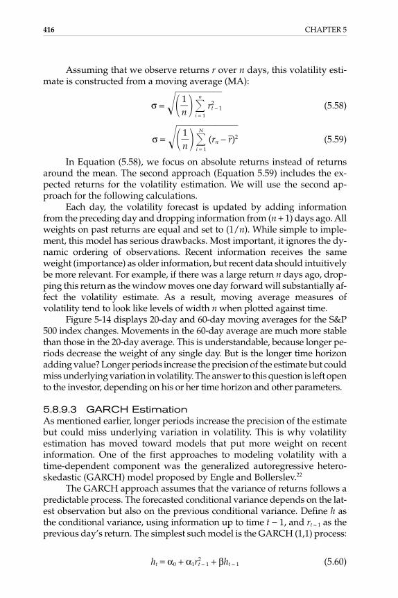
Assuming that we observe returns r over n days, this volatility esti-mate is constructed from a moving average (MA):

σ = �� n

i = 1

r2t − 1 (5.58)

σ = �� N

i = 1

(rn − r�)2 (5.59)

In Equation (5.58), we focus on absolute returns instead of returnsaround the mean. The second approach (Equation 5.59) includes the ex-pected returns for the volatility estimation. We will use the second ap-proach for the following calculations.

Each day, the volatility forecast is updated by adding informationfrom the preceding day and dropping information from (n + 1) days ago. Allweights on past returns are equal and set to (1/n). While simple to imple-ment, this model has serious drawbacks. Most important, it ignores the dy-namic ordering of observations. Recent information receives the sameweight (importance) as older information, but recent data should intuitivelybe more relevant. For example, if there was a large return n days ago, drop-ping this return as the window moves one day forward will substantially af-fect the volatility estimate. As a result, moving average measures ofvolatility tend to look like levels of width n when plotted against time.

Figure 5-14 displays 20-day and 60-day moving averages for the S&P500 index changes. Movements in the 60-day average are much more stablethan those in the 20-day average. This is understandable, because longer pe-riods decrease the weight of any single day. But is the longer time horizonadding value? Longer periods increase the precision of the estimate but couldmiss underlying variation in volatility. The answer to this question is left opento the investor, depending on his or her time horizon and other parameters.

5.8.9.3 GARCH EstimationAs mentioned earlier, longer periods increase the precision of the estimatebut could miss underlying variation in volatility. This is why volatility estimation has moved toward models that put more weight on recent information. One of the first approaches to modeling volatility with atime-dependent component was the generalized autoregressive hetero-skedastic (GARCH) model proposed by Engle and Bollerslev.22

The GARCH approach assumes that the variance of returns follows apredictable process. The forecasted conditional variance depends on the lat-est observation but also on the previous conditional variance. Define h asthe conditional variance, using information up to time t − 1, and rt − 1 as theprevious day’s return. The simplest such model is the GARCH (1,1) process:

ht = α0 + α1r2t − 1 + βht − 1 (5.60)

1�n

1�n

416 CHAPTER 5


The average unconditional variance is found by setting

E[r2t − 1] = ht = ht − 1 = h (5.61)

Solving for h, we find:

h = (5.62)

For this model to be stationary, the sum of parameters α1 + β must beless than unity. This sum is also called the persistence, for reasons that willbecome clear later on. This specification provides a parsimonious model,with few parameters, that seems to fit the data quite well.23

GARCH models have become a mainstay of time series analyses offinancial markets, which systematically display volatility clustering. Liter-ally hundreds of papers have applied GARCH models to stock returndata,24 to interest rate data,25 and to foreign exchange data.26 Econometri-cians have also created many variants of the GARCH model, most ofwhich provide marginal improvement on the original GARCH model. Acomprehensive review of the GARCH literature has been generated by

α0��1 − α1 − β


0%

10%

20%

30%

40%

50%

60%

70%

80%

90%

9/2/

1996

12/2

/199

6

3/2/

1997

6/2/

1997

9/2/

1997

12/2

/199

7

3/2/

1998

6/2/

1998

9/2/

1998

12/2

/199

8

3/2/

1999

6/2/

1999

9/2/

1999

12/2

/199

9

3/2/

2000

6/2/

2000

9/2/

2000

12/2

/200

0

3/2/

2001

6/2/

2001

Vol

atil

ity

Volatility MA(20) Volatility MA(60)

F I G U R E 5-14

Moving Average (MA) Volatility Forecasts for Mexican Peso–U.S. Dollar Foreign Exchange. (Data source: Bloomberg Professional.)


Bollerslev, Chou, and Kroner.27 The drawback of GARCH models is theirnonlinearity. The parameters mentioned earlier must be estimated regu-larly by maximization of the likelihood function, which involves a numer-ical optimization. Typically, researchers assume that the scaled residual

εt =

has a normal distribution.The GARCH approach provides other interesting features. The re-

turns r can be serially uncorrelated but are not independent as they arenonlinearly related through second moments. This class of models is alsorelated to chaos theory. Recent work has revealed that many financialprices display chaotic properties. Often, the nonlinearities behind chaostheory can be traced to the time variation in variances. The GARCH mod-els can explain some of the reported chaotic behavior of financial markets.

Figure 5-15 shows the GARCH forecast of volatility for the S&P 500index changes. It shows increased volatility from fall 1996 on. Afterward,volatility spikes upward during the Asian crisis in summer 1997, the Rus-

rt��ht�

418 CHAPTER 5

0.00%

0.50%

1.00%

1.50%

2.00%

2.50%

3.00%

3.50%

9/6/

1989

3/6/

1990

9/6/

1990

3/6/

1991

9/6/

1991

3/6/

1992

9/6/

1992

3/6/

1993

9/6/

1993

3/6/

1994

9/6/

1994

3/6/

1995

9/6/

1995

3/6/

1996

9/6/

1996

3/6/

1997

9/6/

1997

3/6/

1998

9/6/

1998

3/6/

1999

9/6/

1999

3/6/

2000

9/6/

2000

3/6/

2001

1 SD GARCH volatility forcast

F I G U R E 5-15

GARCH Volatility Forecast for the S&P 500 Index. (Data source: Bloomberg Professional.)


sian crisis in September/October 1998, and the TMT meltdown in April2000 and the months following. A simple Autoregressive Integrated Mov-ing Average (ARIMA) test run on the S&P index (Figure 5-16) shows thatthe assumption of stable volatility is closer to an acceptable level (p value≥ 0.05) in the years until 1996. After 1996, the p values show clearly unac-ceptable low levels.

The practical application of this information is illustrated in Figure5-17, which shows daily returns along with conditional 95 percent confi-dence bands. This model appears to adequately capture variation in risk.Most of the returns fall within the 95 percent band. The few outside thebands correspond to the remaining 5 percent of occurrences.

5.8.9.4 Long-Horizon ForecastsThe GARCH approach can also be used to compute volatility over varioustime horizons. We assume that the volatility is estimated based on dailyinformation. To compute a monthly volatility, we first decompose themultiperiod (geometric) return into daily returns as in Equation (5.63):


Plot of standardized residuals

1990 1992 1994 1996 1998 2000

-8

-4

0

2

4

6

ACF plot of residualsACF

0.0 0.02 0.04 0.06 0.08 0.10 0.12 0.14-1.0

0.0

0.5

1.0

PACF plot of residualsPACF

0.0 0.02 0.04 0.06 0.08 0.10 0.12 0.14

-0.04

0.0

0.04

P values of Ljung-box chi-squared statistics

Lag

p value

0.02 0.03 0.04 0.05 0.06

0.0

0.02

0.04

F I G U R E 5-16

ARIMA Test for S&P 500 Index. (Data source: Bloomberg Professional.)


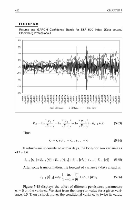
Rt,2 = ln � � = ln � � + ln � � = Rt − 1 + Rt (5.63)

Thus:

rt,T = rt + rt + 1 + rt + 2 + . . . + rT (5.64)

If returns are uncorrelated across days, the long-horizon variance asof t − 1 is:

Et − 1 [rt,T] = Et − 1 [r t2] + Et − 1 [r 2

t + 1] + Et − 1 [r 2t + 2] + . . . + Et − 1 [r 2

T] (5.65)

After some transformation, the forecast of variance τ days ahead is:

Et − 1 [r2t + τ] = α0 + (α1 + β)τ ht (5.66)

Figure 5-18 displays the effect of different persistence parameters α1 + β on the variance. We start from the long-run value for a given vari-ance, 0.5. Then a shock moves the conditional variance to twice its value,

1 − (α1 + β)τ

��1 − (α1 + β)

Pt − 1�Pt − 2

Pt�Pt − 1

Pt�Pt − 2

420 CHAPTER 5

–8%

–6%

–4%

–2%

0%

2%

4%

6%

8%

1/20

/199

34/

20/1

993

7/20

/199

310

/20/

1993

1/20

/199

44/

20/1

994

7/20

/199

410

/20/

1994

1/20

/199

54/

20/1

995

7/20

/199

510

/20/

1995

1/20

/199

64/

20/1

996

7/20

/199

610

/20/

1996

1/20

/199

74/

20/1

997

7/20

/199

710

/20/

1997

1/20

/199

84/

20/1

998

7/20

/199

810

/20/

1998

1/20

/199

94/

20/1

999

7/20

/199

910

/20/

1999

1/20

/200

04/

20/2

000

7/20

/200

010

/20/

2000

1/20

/200

14/

20/2

001

7/20

/200

1

S&P 500 Index 2 SD band –2 SD band

F I G U R E 5-17

Returns and GARCH Confidence Bands for S&P 500 Index. (Data source:Bloomberg Professional.)


1.0. High persistence means that the shock will decay slowly. For instance,with a persistence of 0.986, the conditional variance is still 0.90 after 20days. With a persistence of 0.8, the variance drops very close to its long-run value only after 20 days. The dots on each line represent the averagedaily variance over the following 25 days. High persistence implies thatthe average variance will remain high.

The parabolic shape of the behaving persistence parameters looksvery similar to the cone of forecasted volatilities using the VaR estimatesas calculated with the RiskMetrics approach (see Figure 5-19).

5.8.10 The RiskMetrics Approach

RiskMetrics takes a pragmatic approach to modeling risk.28 Variance fore-casts are modeled using an exponential weighting schema. Formally, theforecast for time t is a weighted average of the previous forecast, usingweight λ (Equation 5.67), and of the latest squared innovation, usingweight (1 − λ) (Equation 5.68):


0 5 10 15 20 25

0.5

1.0 1.00

0.986

0.95

0.900.80

Persistence parameters

Average variancesInitial shock

Forecasting n days ahead

Variance

F I G U R E 5-18

Persistence Parameters on the Variance.


σ = �T

t = 1

(rt − r�)2 (5.67)

σ = (1 − λ)�T

t = 1

λt− 1 (rt − r�)2 (5.68)

In comparing the two estimators (equal and exponential), the ex-ponentially weighted moving average model depends on the parameter0 < λ < 1.

The λ parameter is called the decay factor, and must be less than unity.It determines the relative weights that are applied to the observations (re-turns) and the effective amount of data used in estimating volatility. Thismodel can be viewed as a special case of the GARCH process, where α0 isset to 0 and α1 and β sum to unity. The model therefore allows for persis-tence. As shown in Figure 5-20, it appears to produce results that are veryclose to those achieved with the GARCH model.

1�T

422 CHAPTER 5

1/94 5/94 9/94 1/95

F I G U R E 5-19

S&P 500 Returns and VaR Estimates (1.65σ) (Source: J. P. Morgan, RiskMetricsTechnical Document,” 4th ed., New York: J. P. Morgan, December 1996, chart 5.4.Copyright © 1966 by Morgan Guaranty Trust Company, all rights reserved. Re-production with permission of RiskMetrics Group, LLC.)


A particularly interesting feature of the exponentially weighted esti-mator is that it can be written in a recursive form, which, in turn, will beused as a basis for making volatility forecasts. In order to derive the re-cursive form, it is assumed that an infinite amount of data is available. Forexample, assuming that the sample mean is zero, we can derive the periodt + 1 variance forecast, given data available at time t (one day earlier) as:

σ21,t + 1|t = λσ2

1,t − 1|t + (1 − λ) r 21, t (5.69)

The one-day RiskMetrics volatility forecast is given by:

σ1,t + 1|t = �λσ21,t − 1�|t + (1�− λ) r2

1�,t� (5.70)

The subscript t + 1|t is read “the time t + 1 forecast given informationup to and including time t.” The subscript t − 1 1|t is read in a similar fash-ion. This notation underscores the fact that RiskMetrics is treating thevariance (volatility) as time dependent. The fact that this period’s varianceforecast depends on last period’s variance is consistent with the observedautocorrelation in squared returns. The volatility is given by:


a exp(t)

F I G U R E 5-20

Mean Reversion for the Variance (Source: J. P. Morgan, RiskMetrics TechnicalDocument,” 4th ed., New York: J. P. Morgan, December 1996, chart 5.9. Copy-right © 1996 by Morgan Guaranty Trust Company, all rights reserved. Reproduc-tion with permission of RiskMetrics Group, LLC.)


σ21,t + 1|t = (1 − λ) �

�

i = 0

λir21,t − 1

= (1 − λ)(r21,t + λr2

1,t − 1 + λ2r21,t − 2 + . . .)

= (1 − λ)r21,t + λ(1 − λ)(r2

1,t − 1 + λr21,t − 1 + λ2r2

1,t − 2 + λ2r21,t − 3)

= λσ21,t − 1|t + (1 − λ)r2

1,t (5.71)

The exponential approach is particularly easy to implement becauseit relies on one parameter only and thus is more robust than other modelsto estimation error. In addition, as was the case for the GARCH model, theestimator is recursive; the forecast is based on the previous forecast andthe latest innovation. The whole history is summarized by one number, ht − 1. This is in contrast to the moving average, for example, where the lastn returns must be used to construct the forecast.

The only parameter in this model is the decay factor λ. In theory, thiscould be found by maximizing the likelihood function, but in practice, thiswould be a daunting task to perform every day for all the time series in theRiskMetrics database. In the original technical document, the analysis hasbeen performed on a basic set of core data based on 450 time series. An op-timization has other shortcomings. The decay factor may vary across se-ries and over time, thus decreasing consistency over different periods. Inaddition, different values of λ create incompatibilities for the covarianceterms and may lead to coefficients of correlation greater than unity, as wewill see later. In the original document, RiskMetrics uses only one decayfactor for all series, which is set at 0.94 for daily data. However, RiskMet-rics currently computes stress testing and VaR based on approximately500,000 time series from the DataMetrics platform and allows users to de-fine any combination of decay factors, lookback periods, and time hori-zons, which reflects the underlying data better than the original simplifiedframework. This document also outlines how risk is computed at differentlevels of aggregation (from subposition through the entire portfolio) anddiscusses the various methodologies used (Monte Carlo simulations, his-torical simulations, etc.).29

RiskMetrics also provides risk forecasts over monthly horizons, de-fined as 25 trading days. In theory, the exponential model should be usedto extrapolate volatility over the next day, then the next, and so on untilthe 25th day, as was done previously for the GARCH model (see Figure 5-21). The persistence parameter for the exponential model is unity. There-fore, it is based on the assumption that there is no mean reversion and themonthly volatility should be the same as the daily volatility. In practice,the estimator is identical to the exponentially weighted estimator at the

424 CHAPTER 5


beginning of this section, except that it defines innovations as the 25-dayvariance. After experimenting with the data, J. P. Morgan chose λ = 0.97 asthe optimal decay factor. Therefore, the daily and monthly specificationsare inconsistent with each other. However, they are both easy to use, theyapproximate the behavior of actual data quite well, and they are robust tomisspecifications.

5.8.11 Modeling Correlations

Correlation is of unquestionable importance for portfolio risk—even moreso than individual variances. To illustrate the estimation of correlation, wepick two series: the S&P 500 index and the FTSE 100 index.

Over the period from 1996 to 1998, the average daily correlation co-efficient [MA(60)] was 0.333. However, we should expect some variationin the correlation coefficient because this time period covers the Asian cri-sis and the Russian/LTCM crisis. The average correlation was 0.162 in1995, 0.249 in 1996, 0.305 in 1997, and 0.331 in 1998. As in the case of vari-ance estimation, various methods can be used to capture time variation incorrelation: moving average, GARCH, and exponential.


0.0%

0.5%

1.0%

1.5%

2.0%

2.5%

3.0%

3.5%

1/93

7/93

1/94

7/94

1/95

7/95

1/96

7/96

1/97

7/97

1/98

7/98

1/99

7/99

1/00

7/00

1/01

7/01

Exponential weighted MA(60)

F I G U R E 5-21

Exponential Volatility Forecast for FTSE Index. (Data source: Bloomberg Professional.)


5.8.11.1 Moving AveragesThe first method is based on moving averages (MAs), using a fixed win-dow of length n. Figure 5-22 presents estimates based on an MA(20) andMA(60). Correlations for the MA(20) start around 0.4 and move between0.65 and −0.1 until March 1998, when correlation hits a low of −0.45, mov-ing back to 0.7. The correlation falls from 0.76 at the end of January 1999 to−0.34 by April 21, 1999. As can be seen in the figure, the MA(60) followswith some lag and averaging of the swings. These estimates are subject tothe same criticisms as before. Moving averages place the same weight onall observations within the moving window and ignore the fact that morerecent observations may contain more relevant information than olderones. In addition, dropping observations from the window sometimes hassevere effects on the measured correlation.

5.8.11.2 Exponential AveragesIn theory, GARCH estimation could be extended to a multivariate frame-work. The problem is that the number of parameters to estimate increasesexponentially with the number of series. With two series, for instance, weneed to estimate nine terms, or three α1, α0, and β parameters for each of

426 CHAPTER 5

-0.6

-0.4

-0.2

0.0

0.2

0.4

0.6

0.8

1.0

7/15

/199

6

10/1

5/19

96

1/15

/199

7

4/15

/199

7

7/15

/199

7

10/1

5/19

97

1/15

/199

8

4/15

/199

8

7/15

/199

8

10/1

5/19

98

1/15

/199

9

4/15

/199

9

7/15

/199

9

10/1

5/19

99

1/15

/200

0

4/15

/200

0

7/15

/200

0

10/1

5/20

00

1/15

/200

1

4/15

/200

1

7/15

/200

1

Cor

rela

tion

SPX

/UK

X

MA(20) MA(60)

F I G U R E 5-22

Moving Average–Based Correlation Between the S&P 500 Index and the FTSE100 Index. (Data source: Bloomberg Professional.)


the three covariance terms. For larger samples of securities, this numberquickly becomes unmanageable.

The RiskMetrics approach is convincing in its simplicity. Covari-ances are estimated, much like variances, using an exponential weightingscheme:

h12,t = λh12,t − 1 + (1 − λ)r1,t − 1r2,t − 1 (5.72)

As before, the decay factor λ is arbitrarily set at 0.94 for daily dataand 0.97 for monthly data. The conditional correlation is then:

ρ12,t = (5.73)

Figure 5-23 displays the time variation in the correlation between theS&P 500 index and the FTSE 100 index. The pattern of movements in cor-relations does not seem too different from the MA model, plotting some-where between the MA(20) and MA(60).

h12,t��h1,th2,t�


-1

-0.8

-0.6

-0.4

-0.2

0

0.2

0.4

0.6

0.8

1

7/15

/199

6

10/1

5/19

96

1/15

/199

7

4/15

/199

7

7/15

/199

7

10/1

5/19

97

1/15

/199

8

4/15

/199

8

7/15

/199

8

10/1

5/19

98

1/15

/199

9

4/15

/199

9

7/15

/199

9

10/1

5/19

99

1/15

/200

0

4/15

/200

0

7/15

/200

0

10/1

5/20

00

1/15

/200

1

4/15

/200

1

Cor

rela

tion

SP

X/U

KX

Exponential weighted

F I G U R E 5-23

Exponential-Weighted Correlation Between the S&P 500 Index and the FTSE 100Index. (Data source: Bloomberg Professional.)


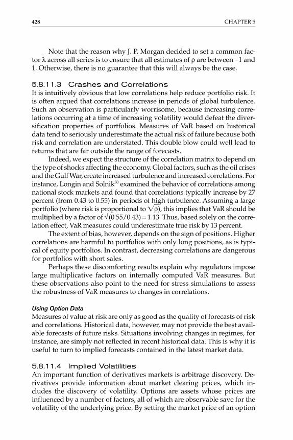
Note that the reason why J. P. Morgan decided to set a common fac-tor λ across all series is to ensure that all estimates of ρ are between −1 and1. Otherwise, there is no guarantee that this will always be the case.

5.8.11.3 Crashes and CorrelationsIt is intuitively obvious that low correlations help reduce portfolio risk. Itis often argued that correlations increase in periods of global turbulence.Such an observation is particularly worrisome, because increasing corre-lations occurring at a time of increasing volatility would defeat the diver-sification properties of portfolios. Measures of VaR based on historicaldata tend to seriously underestimate the actual risk of failure because bothrisk and correlation are understated. This double blow could well lead toreturns that are far outside the range of forecasts.

Indeed, we expect the structure of the correlation matrix to depend onthe type of shocks affecting the economy. Global factors, such as the oil crisesand the Gulf War, create increased turbulence and increased correlations. Forinstance, Longin and Solnik30 examined the behavior of correlations amongnational stock markets and found that correlations typically increase by 27percent (from 0.43 to 0.55) in periods of high turbulence. Assuming a largeportfolio (where risk is proportional to �ρ�), this implies that VaR should bemultiplied by a factor of √(0.55/0.43) = 1.13. Thus, based solely on the corre-lation effect, VaR measures could underestimate true risk by 13 percent.

The extent of bias, however, depends on the sign of positions. Highercorrelations are harmful to portfolios with only long positions, as is typi-cal of equity portfolios. In contrast, decreasing correlations are dangerousfor portfolios with short sales.

Perhaps these discomforting results explain why regulators imposelarge multiplicative factors on internally computed VaR measures. Butthese observations also point to the need for stress simulations to assessthe robustness of VaR measures to changes in correlations.

Using Option DataMeasures of value at risk are only as good as the quality of forecasts of riskand correlations. Historical data, however, may not provide the best avail-able forecasts of future risks. Situations involving changes in regimes, forinstance, are simply not reflected in recent historical data. This is why it isuseful to turn to implied forecasts contained in the latest market data.

5.8.11.4 Implied VolatilitiesAn important function of derivatives markets is arbitrage discovery. De-rivatives provide information about market clearing prices, which in-cludes the discovery of volatility. Options are assets whose prices areinfluenced by a number of factors, all of which are observable save for thevolatility of the underlying price. By setting the market price of an option

428 CHAPTER 5


equal to its model value, one can recover an implied volatility.31 Similarly,implied correlations also can be derived from triplets of options, using, forinstance, the Margrabe pricing model.32

Correlations are also implicit in so-called quanto options, which alsoinvolve two random input variables. For instance, a quantity-adjusted op-tion would be an option struck on a foreign stock index where the foreigncurrency payoff is translated into dollars at a fixed rate. The valuation for-mula for such an option also involves the correlation between two sourcesof risk. Thus, options can potentially reveal a wealth of information aboutfuture risks and correlations.

If options markets are efficient, the implied volatility should providethe market’s best estimate of future volatility. However, options tradingmeans taking volatility bets. Expressing a view on volatility has become sopervasive in the options markets that prices are often quoted in terms ofbid-ask volatility. As options reflect the market consensus about futurevolatility, there are sound reasons to believe that options-based forecastsshould be superior to historical estimates.

The empirical evidence indeed points to the superiority of optionsdata. An intuitive way to demonstrate the usefulness of options data is toanalyze the Russian crisis in September to October 1998. Figure 5-24 com-


0%

5%

10%

15%

20%

25%

30%

35%

40%

45%

7/15

/199

6

10/1

5/19

96

1/15

/199

7

4/15

/199

7

7/15

/199

7

10/1

5/19

97

1/15

/199

8

4/15

/199

8

7/15

/199

8

10/1

5/19

98

1/15

/199

9

4/15

/199

9

7/15

/199

9

10/1

5/19

99

1/15

/200

0

4/15

/200

0

7/15

/200

0

10/1

5/20

00

1/15

/200

1

4/15

/200

1

7/15

/200

1

Implied volatility

F I G U R E 5-24

Implied Volatility Forecasts for S&P Index Returns. (Data source: Bloomberg Professional.)


pares volatility forecasts during 1992, including those implied from S&P500 index options and a moving average with a window of 60 days. It is in-tuitively obvious that the implied volatility immediately picks up the be-havior of the market and reflects the expected volatility to justify currentmarket conditions. As options traders rationally anticipated greater turbu-lence, the implied volatility was much more useful than time series models.

5.8.11.5 ConclusionsThe empirical evidence shows that options contain a wealth of informationabout price risk that is generally superior to time-series models. This find-ing is particularly useful in times of stress, when the market has access tocurrent information that is simply not reflected in historical approaches.The drawback of option-implied parameters is that the volume and rangeof traded options is not sufficiently wide to cover the volatility of all essen-tial financial prices. As more and more options contracts and exchanges arespringing up all over the world, traded options data is more readily avail-able. Historical data provides a backward-looking alternative.

The options-based credit model detailed in Section 5.8.11.4 high-lights the advantages of an options-based approach:

• Using implied volatilities, the options-based model is forwardlooking and can be applied in a similar context as the marketrisk–based options model regarding time horizon.

• The options model does not necessarily require a mean variancenormal distribution. Nonlinearity of the underlying asset iscaptured with an options-based approach for market and creditrisk. Operational risk issues can be approached and covered in asimilar manner, based on the evaluation of the implied volatilityrequired to calculate the operational risk premium for thehistorical operational losses as captured through a historicaloperational risk database.

5.9 LIQUIDITY RISK

The approaches for market risk management under normal conditions tra-ditionally have focused on the distribution of portfolio value changes re-sulting from moves in the midprice. Under this assumption, market risk isreally in a “pure” form: risk in an idealized market with no “friction” in ob-taining a fair price. However, many markets possess an additional liquid-ity component that arises from a trader not realizing the midprice whenliquidating a position, but rather the midprice minus the bid-ask spread.

We argue that liquidity risk associated with the uncertainty of thespread, particularly for thinly traded or emerging market securities underadverse market conditions, is an important part of overall risk and therefore

430 CHAPTER 5


an important component and a critical assumption of modeling. The currentregulative conceptual approach to measuring market risk does not considerliquidity risk explicitly. Approaches have been developed for modeling li-quidity risk that can be easily and seamlessly integrated into standard VaRmodels.33 The BIS is inadvertently monitoring liquidity risk, but by notmodeling it explicitly and therefore capitalizing against it. Therefore, bankswill be experiencing surprisingly many violations of capital requirements,particularly if their portfolios are concentrated in emerging markets. Thecrash in October 1998 has shown the impact of inadequate liquidity in Rus-sian bonds and the supposed adequacy of quantitative models.

Portfolios are usually marked to market at the middle of the bid-offerspread, and many hedge funds used models that incorporated this assump-tion. In late August, there was only one realistic value for the portfolio: thebid price. Amid such massive sell-offs, only the first seller obtains a reason-able price for its security; the rest lose a fortune by having to pay a liquiditypremium if they want a sale. . . . Models should be revised to include bid-offer behavior.34

The turmoil in the capital markets in October 1998 led experts andlaymen alike to cast liquidity risk in the role of the culprit. Inexperiencedand sophisticated players alike were caught by surprise when marketsdried up. Unsurprisingly, the first to go were the emerging markets inAsia, and, more recently, in Russia. Then the crisis spilled over into theU.S. corporate debt market, which was indeed much more surprising. Oneof the most famous victims of the 1998 liquidity crisis was Long Term Cap-ital Management (LTCM). Spreads appeared to widen out of the blue; butthis could have been predicted. More generally, it is a well-acknowledgedfact that the standard VaR concept used for measuring both market andcredit risk for tradable securities lacks a rigorous treatment of liquidityrisk. At best, the risk for large illiquid positions is adjusted upward in anad hoc fashion by utilizing a longer time horizon in the calculation of VaRthat at best is a subjective estimate of the likely liquidation time of the po-sition. But this holding period adjustment is usually carried out using thesquare root of time scaling of the variances and covariances rather than arecalculation of variances and covariances for the longer time horizon.35

The combination of the recent rapid expansion of emerging markettrading activities and the recurring turbulence in those markets haspushed liquidity risk to the forefront of market risk management research.New work in asset pricing has demonstrated how liquidity as a drivingfactor in risk measurement plays a key role in security valuation and opti-mal portfolio choice by effectively imposing endogenous borrowing andshort-selling constraints, as argued by Longstaff.36

Liquidity also plays a major role in transaction costs, as trades of largeilliquid positions typically execute at a price away from the midprice.



BARRA’s Market Impact Model and other such models quantify the marketimpact cost, defined as the cost of immediate execution, for establishing andliquidating large positions. Jarrow and Subramanian consider the effect oftrade size and execution lag on the liquidation value of the portfolio,37 pro-posing a liquidity-adjusted VaR measure that incorporates a liquidity dis-count, volatility of the liquidity discount, and volatility of the time horizonto liquidation. Although this concept is attractive, there is no available dataor procedure to measure the model parameters such as mean and variancesfor quantity discounts or execution lags for trading large blocks.

Illiquidity can arise from different sources. Conceptually we have todistinguish between risk caused by uncertainty in asset returns and riskdue to liquidity constraints. The breakdown of liquidity risk allows a dis-tinction between exogenous liquidity risk, which is not under control ofthe market participant (market maker or trader), and endogenous liquid-ity risk, which is the under control of the trader and usually the result ofsudden unloading of large positions that the market is unable to absorb ef-ficiently. Conceptually, the current models (which do not distinguish be-tween uncertainty from asset returns or due to liquidity) ignore valuableinformation contained in the distribution of bid-ask spreads.

Traditional market risk management (under normal conditions) usu-ally deals exclusively with the distribution of portfolio value changes viathe distribution of asset/trading returns. These asset/trading returns arebased on the midprice, and thus the market risk is really in a “pure”form—risk in an idealized market with no friction in obtaining the fairprice. However, many markets possess an additional liquidity componentthat arises from traders not realizing the midprice when liquidating a po-sition quickly or when the market is moving against them; instead, theyrealize the midprice minus some spread. Marking to market thereforeyields an underestimation of the true risk in such markets, because the re-alized value on liquidation can deviate significantly from the market mid-price. We argue that the deviation of this liquidation price from themidprice, also referred to as the market impact or liquidation cost, and thevolatility of this cost, are important components to model in order to cap-ture the true level of overall risk. We conceptually split uncertainty in market value of an asset, i.e., its overall market risk, into two parts: (1) uncertainty that arises from asset returns, which can be thought of as apure market risk component, and (2) uncertainty due to liquidity risk.

Conventional VaR approaches, such as J. P. Morgan’s RiskMetrics,focus on capturing risk due to uncertainty in asset returns but ignore uncer-tainty due to liquidity risk. The liquidity risk component is concerned withthe uncertainty of liquidation costs. Conceptually, we can express theseideas as a market/liquidity risk plane that considers the joint impact of thetwo types of risk. Most markets and trading situations fall into regions 1 and3; we observe that market risk and liquidity risk components are correlated

432 CHAPTER 5


in most cases. For instance, FX derivative products in emerging marketshave high market and liquidity risks and therefore fall into region 1. Thespot markets for most G-7 currencies, on the other hand, will fall into region3 due to the relatively low market and liquidity risks involved. Most normaltrading activity occurs in these two regions and is subject to exogenous li-quidity risk, which refers to liquidity fluctuations driven by factors beyondindividual traders’ control. We distinguish this from endogenous liquidityrisk, which refers to liquidity fluctuations driven by individual actions, suchas an attempt to unwind a very large position. A trader holding a very largeposition in an otherwise stable market, for example, may find him- or her-self in region 4. The risk plane (market/liquidity risk) is of course a simpli-fication of a more complex relationship between markets and position sizes,involving both exogenous and endogenous components of liquidity risk. Inparticular, creating movement along the liquidity axis can be done by mov-ing either across established or emerging markets (i.e., increasing exoge-nous illiquidity) or within a market by simply increasing one’s position size(i.e., increasing endogenous illiquidity).

Exogenous illiquidity is the result of market characteristics; it is com-mon to all market players and unaffected by the actions of any one partic-ipant (although it can be affected by the joint action of all or almost allmarket participants, as happened in several markets in the summer of1998). The market for liquid securities, such as G-7 currencies, is typicallycharacterized by heavy trading volumes, stable and small bid-askspreads, and stable and high levels of quote depth. Liquidity costs may benegligible for such positions when marking to market provides a properliquidation value. In contrast, markets in emerging currencies or thinlytraded junk bonds are illiquid and are characterized by high volatilities ofspread, quote depth, and trading volume. Endogenous illiquidity, in con-trast, is specific to one’s position in the market and varies across marketparticipants, and the exposure of any one participant is affected by his orher actions. Endogenous illiquidity is mainly driven by the size of the po-sition: the larger the size, the greater the endogenous illiquidity. A goodway to understand the implications of position size is to consider thequote depth, which is the relationship between the liquidation price andthe total position size held. Quote depth is defined as the volume of sharesavailable at the market maker’s quoted price (bid or ask). Market impactmodels such as one developed by BARRA quantify this relationship be-tween the transaction price and trade size. If the market order to buy orsell is smaller than the volume available in the market at the quote, thenthe order transacts at the quote. In this case the market impact cost, de-fined as the cost of immediate execution, will be half of the bid-ask spread.In our framework, such a position only possesses exogenous liquidity riskand no endogenous risk. If the size of the order exceeds the quote depth,the cost of market impact will be higher than the half-spread. The differ-



ence between the total market impact and half-spread is called the incre-mental market cost, and constitutes the endogenous liquidity component inour framework. Endogenous liquidity risk can be particularly importantin situations where normally fungible market positions cease to be fungi-ble; a good example would be when the cheapest-to-deliver bond of a fu-tures contract switches. The cheapest-to-deliver bond is a bond that hasthe same profile as the bonds used in the futures contract. Once the cheapest-to-deliver bond changes in profile, for example because durationis getting shorter because maturity is getting closer, this specific cheapest-to-deliver bond is no longer a fungible position. Later, when the bond ispaid back, it disappears from the market. But the futures contract is still inthe market. The bonds in the futures contract have to be “switched” fromtime to time to reflect the correct profile in the contract.

Quantitative methods for modeling endogenous liquidity risk haverecently been proposed by Jarrow and Subramanian,38 Chriss and Alm-gren,39 Bertsimas and Lo,40 and Campbell et al.41 Jarrow and Subramanian,for example, consider optimal liquidation of an investment portfolio overa fixed horizon. They characterize the costs and benefits of block sale ver-sus slow liquidation and propose a liquidity adjustment to the standardVaR measure. The adjustment, however, requires knowledge of the rela-tionship between the trade size and both the quantity discount and the ex-ecution lag. Clearly, there is no readily available data source forquantifying those relationships, which forces one to rely on subjective es-timates. In this work we approach the liquidity risk problem from theother side, focusing on methods for quantifying exogenous rather than en-dogenous liquidity risk. The purpose is to consider two key facts in theliquidity discussion. First, fluctuations in exogenous liquidity risk areoften large and important, as is clear from our empirical examples, andthey are relevant for all market players, whether large or small. Second, insharp contrast to the situation for endogenous liquidity risk, the dataneeded to quantify exogenous liquidity risk is widely available. This is be-cause exogenous liquidity risk is characterized by the volatility of the ob-served spread with no reference to the relationship of the realized spreadto trade size. The upshot is that we can incorporate liquidity risk into VaRcalculations in a simple and straightforward way.

Traditional VaR measures are obtained from the distribution of port-folio returns computed at the bid-ask average prices. This implies that thepositions can be liquidated at bid-ask prices. This approach conceptuallyunderestimates risk by neglecting the practical fact that liquidation doesnot occur at the bid-ask average price, but rather at the bid-ask average lesshalf the spread. Thus the spread may fluctuate widely. Use of a simplemeasure of exogenous liquidity risk, computed using the distribution ofobserved bid-ask spreads, results in much more appropriate risk result,particularly in emerging market securities. What is the impact for the reg-

434 CHAPTER 5


ulatory capitalization of a trading operation? BIS regulations stipulatemonitoring of only the number of VaR violations, not of the way that VaRis computed. Neglecting liquidity risk will lead to underestimation of over-all risk, undercapitalization, and too many violations. The BIS regulation,whether intentionally or not, monitors liquidity risk quite appropriately inrelation to the qualitative aspects of the regulation. Performance evaluationshould also be based on returns adjusted for risk—including liquidity risk.Some financial institutions do this, and due to higher margins many finan-cial institutions have seen growth in their emerging market trading activ-ity. A risk-adjusted view of performance in those markets should accountnot only for market risk but also for liquidity risk. Otherwise, performancewill not be assessed correctly and dealer compensation for liquidity riskwill be distorted as it is not under the control of the dealer.

5.10 SUMMARY

The integration of the different risk categories depends on the compatibil-ity of approaches, methodologies, and parameters. Credit risk in the formof specific risks is integrated with market risk in the form of company-specific spread adjustments on top of the generic treasury yield curves, re-flecting the company-specific (credit) risk. As discussed in this chapter,the integration of credit and market risk models is more challenging. Thisis partly due to the fact that the BIS adds values together, ignoring the factthat the underlying valuation models have different roots, assumptions,and parameters. The frequency of the credit events (up- or downgrades)and subsequently the price adjustment follows a different rhythm thanmarket risk valuation, where daily pricing allows a daily frequency. Thistopic is discussed in Secs. 3.6 to 3.8. For some time, VaR was a favoritemeasurement approach for everybody and anything. However, more andmore, the practical relevance outweighs the fanciness of valuation. Thedifferent valuation methodologies, including the advantages and thedrawbacks, are discussed to highlight which areas they fit best. Stress test-ing and limitations of VaR are discussed in detail, emphasizing the impor-tant fact that the interpretation of VaR data becomes meaningless unlessthe relevance of the valuation models, parameters, and assumptions is re-examined on a regular basis. The relevance includes stability of distribu-tions and volatilities including correlations and time-varying risk.Liquidity risk is discussed in detail, as it affects market, credit, and opera-tional risks simultaneously. Market prices react with widening spreads,credit risk reacts with higher specific risks, and operational risk is affectedto exposed transaction settlements.

This chapter presents a critical review of many aspects of the previ-ous chapters. It is important to note that technology has helped to inte-grate market, credit, and operational risk via higher processing capacities,



networks and shared information, and the increased rapidity with whichcompanies can close their books and P&L statements. Relevant informa-tion for credit risk valuation is disclosed more frequently, which is re-flected in more frequent adjustments of credit risk valuations. Systemicrisk is becoming more important. Despite the gap between market andcredit risk categories, unusual market and credit behavior can trigger sys-temic risk in a significant way given technology and information net-works that spread information in real time. One historical example ofsystemic risk is the Russian crisis of 1998.

5.11 NOTES

1. Bank for International Settlement (BIS), Basel Committee on BankingSupervision, The New Basel Capital Accord: Consultative Document, Issued forComment by 31 May 2001, Basel, Switzerland: Bank for InternationalSettlement, January 2001.

2. Ibid.

3. The committee will release a complete and fully specified proposal for anadditional round of consultation in early 2002 and will finalize the newaccord during 2003. The Basel Committee envisions an implementation dateof 2005 for the new accord. See Bank for International Settlement (BIS),Basel Committee on Banking Supervision, “Update on the New BaselCapital Accord,” press release, Basel, Switzerland: Bank for InternationalSettlement, June 25, 2001.

4. Bank for International Settlement (BIS), Basel Committee on BankingSupervision, Amendment to the Capital Accord to Incorporate Market Risks,Basel, Switzerland: Bank for International Settlement, January 1996,modified September 1997.

5. Bank for International Settlement (BIS), Basel Committee on BankingSupervision, A New Capital Adequacy Framework, Basel, Switzerland: Bankfor International Settlement, June 1999.

6. Bank for International Settlement (BIS), Basel Committee on BankingSupervision, “Progress Towards Completion of the New Basel CapitalAccord,” press release, Basel, Switzerland: Bank for InternationalSettlement, December 13, 2001.

7. Bank for International Settlement (BIS), Basel Committee on BankingSupervision, “Quantitative Impact Survey of New Basel Capital Accord,”press release, Basel, Switzerland: Bank for International Settlement, October1, 2002.

8. Bank for International Settlement (BIS), Basel Committee on BankingSupervision, “Update on the New Basel Capital Accord,” press release,Basel, Switzerland: Bank for International Settlement, June 25, 2001;“Update on the New Basel Capital Accord, Issue 2,” press release, Basel,Switzerland: Bank for International Settlement, September 21, 2001; Resultsof the Second Quantitative Impact Study, Basel, Switzerland: Bank for

436 CHAPTER 5


International Settlement, November 5, 2001; Potential Modifications to theCommittee’s Proposals, Basel, Switzerland: Bank for International Settlement,November 5, 2001; The Quantitative Impact Study for Operational Risk:Overview of Individual Loss Data and Lessons Learned, Basel, Switzerland: Bankfor International Settlement, January 2002.

9. Bank for International Settlement (BIS), Basel Committee on BankingSupervision, Results of the Second Quantitative Impact Study, Basel,Switzerland: Bank for International Settlement, November 5, 2001.

10. Bank for International Settlement (BIS), Basel Committee on BankingSupervision, The Quantitative Impact Study for Operational Risk: Overview ofIndividual Loss Data and Lessons Learned, Basel, Switzerland: Bank forInternational Settlement, January 2002.

11. Ibid.

12. Bank for International Settlement (BIS), Basel Committee on BankingSupervision, The New Basel Capital Accord: Consultative Document, Issued forComment by 31 May 2001, Basel, Switzerland: Bank for InternationalSettlement, January 2001, para. 19ff.

13. Ibid., para. 586 ff.

14. Ibid., para. 633 ff.

15. The latest approved version, dated May 20, 2001, is officially titled “AIMR-PPS Standards, the U.S. and Canadian Version of GIPS.” For details, seewww.aimr.org/pdf/gips.pdf andwww.aimr.com/standards/pps/pps.html#new.

16. See Anil Bangia, Francis X. Diebold, Til Schuermann, and John D.Stroughair, Modeling Liquidity Risk, with Implications for Traditional MarketRisk Measurement and Management, University of Pennsylvania, FinancialInstitutions Center, The Wharton School, June, 1999.

17. See for instance E. I. Altman and D. L. Kao, “Examining and ModelingCorporate Bond Rating Drift,” working paper, New York UniversitySalomon Center, New York, 1991. These researchers find that there ispositive autocorrelation in S&P downgrades, so a downgrade implies ahigher likelihood of a downgrade in the following period. Looking at theS&P rating data, the study finds that an upgrade tends to lead to a “quiet”period. However, this finding applies in particular to the S&P ratingmethodology. Other credit rating systems are not necessarily subject to thisproblem in the same way given different assumptions and approaches.

18. Bank for International Settlement (BIS), Basel Committee on BankingSupervision, Amendment to the Capital Accord to Incorporate Market Risks,Basel, Switzerland: Bank for International Settlement, January 1996,modified September 1997, para. B4.h.

19. See www.bog.frb.fed.us/BoardDocs/Testimony/1998/19981001.html.

20. For an analysis of this “fallacy,” see R. Merton and P. Samuelson, “Fallacy ofthe Log-Normal Approximation to Portfolio Decision-Making over ManyPeriods,” Journal of Financial Economics 1 (1974), 67–94; or W. Harlow, “Asset



Allocation in a Downside Risk Framework,” Financial Analysts Journal 47(September 1991), 28–40.

21. Other approaches exist, however. See for instance J. Boudoukh, M.Richardson, and R. Whitelaw, “Expect the Worst,” Risk (September 1995),101–105, which describes multivariate density estimation as anonparametric model that appears to be quite flexible. Also, risk estimatorsdo not necessarily have to rely solely on daily closing prices. Parkinson hasshown that using the information in the extreme values (daily high andlow) leads to an estimator that is twice as efficient as the usual volatility. Fordetails see M. Parkinson, “The Extreme Value Method for Estimating theVariance of the Rate of Return,” Journal of Business 53 (1980), 61–65.

22. For details, see R. Engle, “Auto-regressive Conditional Heteroskedasticitywith Estimates of the Variance of United Kingdom Inflation,” Econometrica50 (1982), 987–1007; and T. Bollerslev, “Generalized Auto-regressiveConditional Heteroskedasticity,” Journal of Econometrics 31 (1986), 307–327.

23. For an analysis of the theoretical rationale behind the success of GARCHmodels, see D. Nelson, “ARCH Models as Diffusion Approximations,”Journal of Econometrics 45 (1990), 7–38.

24. K. French, W. Schwert, and R. Stambaugh, “Expected Stock Returns andVolatility,” Journal of Financial Economics 19 (1987), 3–29.

25. R. Engle, D. Lilien, and R. Robins, “Estimating Time-Varying Risk Premia inthe Term Structure: The ARCH-M Model,” Econometrica 55 (1987), 391–407.

26. D. Hsieh, “The Statistical Properties of Daily Foreign Exchange Rates:1974–983,” Journal of International Economics 24 (1988), 129–145; A.Giovannini and R. Jorion, “The Time-Variation of Risk and Return in theForeign Exchange and Stock Markets,” Journal of Finance 44 (1989), 307–325.

27. T. Bollerslev, R. Chou, and K. Kroner, “ARCH Modelling in Finance: AReview of the Theory and Empirical Evidence,” Journal of Econometrics 52(1992), 5–59.

28. For more details on the methodology, see J. P. Morgan, RiskMetrics TechnicalDocument, 4th ed., New York: J. P. Morgan, December 17, 1996, p. 78.

29. The methods for incorporating this data are fully discussed in Jorge Minaand Jerry Yi Xiao, Return to RiskMetrics: The Evolution of a Standard, NewYork: RiskMetrics Group, 2001.

30. Francis Longin and Bruno Solnik, “Is the Correlation in International EquityReturns Constant: 1960–1990?” Journal of International Money and Finance 14(1995), 3–26.

31. One potential objection to the use of option volatilities is that the Black-Scholes model is, strictly speaking, inconsistent with stochastic volatilities.However, recent research on the effect of stochastic volatilities has shownthat the Black-Scholes model performs well for short-term at-the-moneyoptions. For further details, see S. Heston, “A Closed-Form Solution forOptions with Stochastic Volatility with Applications to Bond and CurrencyOptions,” Review of Financial Studies 6 (1993), 327–343; J. Duan, “TheGARCH Option Pricing Model,” Mathematical Finance 5 (1995), 13–32; D.

438 CHAPTER 5


Duffie and D. Lando, “Term Structures of Credit Spreads with IncompleteAccounting Information,” working paper, Stanford University GraduateSchool of Business, 1997; and D. Bates, “Testing Option Pricing Models,”Working Paper NBER-5129, Cambridge, MA: National Bureau of EconomicResearch, 1995.

32. W. Margrabe, “The Value of an Option to Exchange One Asset for Another,”Journal of Finance 33 (1978), 177–186.

33. Anil Bangia, Francis X. Diebold, Til Schuermann, and John D. Stroughair,Modeling Liquidity Risk, with Implications for Traditional Market RiskMeasurement and Management, University of Pennsylvania, FinancialInstitutions Center, The Wharton School, June 1999.

34. Nicholas Dunbar, “Meriwether’s Meltdown,” Risk (October 1998), 32–36.

35. For a discussion on the appropriateness of the time-scaling of variances, seeF. X. Diebold, A. Hickman, A. Inoue, and T. Schuermann, “Scale Models,”Risk 11 (January 1998), 104–107.

36. Francis A. Longstaff, “Optimal Portfolio Choice and Valuation of IlliquidSecurities,” manuscript, UCLA, Department of Finance, Los Angeles, 1998.

37. R. A. Jarrow and A. Subramanian, “Mopping up Liquidity,” Risk 10(December 1997), 170–173.

38. Ibid.

39. N. Chriss and R. Almgren, “Optimal Liquidation,” manuscript, Universityof Chicago, Department of Mathematics, Goldman Sachs & Co., andCourant Institute of Mathematical Sciences, 1998.

40. D. Bertsimas and A. W. Lo, “Optimal Control of Execution Costs,” Journal ofFinancial Markets 1 (1998), 1–50.

41. J. Y. Campbell, A. W. Lo, and A. C. MacKinlay, The Econometrics of FinancialMarkets, Princeton, NJ: Princeton University Press, 1997.



C H A P T E R 6

Case Studies

6.1 STRUCTURE OF STUDIES

At present, there are standard industry-accepted definitions for market,credit, and systemic risk, but no such definition for operational risk. (TheBIS definition of operational risk is not accepted throughout the industry.)For these case studies, therefore, we use the definitions and frameworkfrom Chapter 5 and verify case by case the extent to which the structure ofthis approach can be applied.

The first section of each case study describes the causal events andcontributory factors leading to losses at a given financial institution. Thefollowing section outlines the effect of the causal events and contributoryfactors in order to clearly separate the causes, symptoms, and main andside effects. The final section allocates the different findings to the riskareas being affected. This section is key and will highlight to which areasthe losses have to be allocated and why management and/or regulatorycontrols failed.

6.2 OVERVIEW OF CASES

The list of crises, near collapses, and effective collapses involving financialinstitutions is endless. However, some cases catch the attention of the regulators, and especially the media, and thus drive developments andtrigger the implementation of new regulations. This in turn forces the in-dustry to develop new approaches and new processes. Table 6-1 providesan overview of recent incidents in the market. Other cases, such as thelosses and consequent shutdown of the London-based Griffin Trading

441



442

T A B L E 6-1

Overview of Recent Incidents in Financial Institutions

Institution Date Cause Effect

Banco Ambrosiano 1982 Money laundering; fraud; conspiracy leading to Loss of $1.4 billionmultiple murders; complex networking of criminal elements including P2 members, Vatican officials, and high-ranking politicians in many countries.3

Bankers Trust October 27, 1994 Material misrepresentations and omissions to $195 million damage; bankruptcy as client; lawsuits filed by Procter & Gamble and clients moved business to other banks;Gibson Greetings.4 takeover in 1999 through Deutsche Bank

Barings February 23, 1995 Unauthorized trading; failure of controls; lack of Loss of $1.328 billion; bankruptcyunderstanding of the business, particularly in (takeover)futures; carelessness in the internal auditdepartment.

BCCI 1991 Weak credit analysis process; missing or Collapse; $500 billion in estimatedincomplete loan documentation; concealment damage to taxpayersand fraud across the institution; money laundering.5

Bre-X November 5, 1997 Deliberate stock manipulation through false Loss of $120 millionclaims of gold discovery.6

Credit Lyonnais 1994 Inadequate supervision and deregulation Loss of accumulated $24.22 billion;supported fraud; loan mismanagement; collapse without governmental supportmoney laundering; fraud; complex networking of politicians, bankers, and new owners.7

Daiwa July 1995 Unauthorized trading of U.S. bonds and Loss of $1.1 billionaccumulated losses over 12 years.8


443

Drexel Burnham Lambert February 9, 1990 Growth and profit were tied to the junk bond market $1.3 billion global settlement case;Drexel had created and that crashed. The company $200 million criminal fine; $400 millionwas highly leveraged with substantial unsecured civil restitution fund with SEC; bankruptcyshort-term borrowing at holding company. Drexel did not and could not obtain committed bank lines of credit to support the unsecured borrowing positions.

Jardine Fleming July 1995 Lax controls; fraud; insider trading; selective Compensation of $19.3 million to client deal allocations to client account.9 with impacted performance from

selective deal allocation; $2.2 million missing from client account

Kidder Peabody April 1994 Phony profits; superiors did not understand Loss of $350 milliontrades; no questions asked because profits were being produced; inadequate supervision;promotion of superstar culture; employmentreferences not checked; payment of bogus bonuses.10

LTCM September 1998 Growth and profit were tied to leverage and large Loss of $3.5 billion;exposures to illiquid emerging market exposures. investment ofThe company was highly leveraged with substantial additional $1 millionunsecured short-term borrowing at holding company. by syndicate ofNo questions were asked because profits were being borrowers to avoidproduced. Inadequate supervision; promotion of crash and systemicsuperstar culture (including Nobel Prize winners). crisis; retirement ofLTCM did not and could not sell illiquid positions to chairman of UBSsupport the unsecured borrowing positions as the market went down and investors sold shares of LTCM.


444

Institution Date Cause Effect

Metallgesellschaft December 1993 Hedge strategies for oil prices; incorrect economic Loss of $1.5 billionassumptions. Liquidation of positions failed, strategies led to fraud.

Morgan Grenfell September 2, 1996 Inadequate supervision; promotion of superstar Loss of $260 millionculture; no questioning of profits and instruments used.11

Nasdaq May 1994 Between 1989 and 1994, several brokers kept Payment by clients of a spread kept atspread above unnaturally high levels and unnaturally high levelsgenerated excessive profits for themselves and their institutions. Article in Journal of Financedisclosed excess profits from spread and initiated SEC investigation.12

NatWest 1996 Rogue trading; fraud.13 Loss of £90.3 million

Orange County, California December 1994 Illegal use of state funds; losses from bond trading; Loss of $164 million; bankruptcyfalse and misleading financial statements; fraud.14

Sumitomo June 13, 1995 Copper trading errors; failure to segregate duties; Loss of $2.6 billionno questions asked because profits were produced;inadequate supervision; promotion of superstar culture.

T A B L E 6-1

Overview of Recent Incidents in Financial Institutions (Continued )


company1 and of Cendant,2 or fraud charges against Martin Frankel, arenot analyzed. The cases of Metallgesellschaft, Sumitomo, LTCM, and Bar-ings have been selected for detailed analysis.

6.3 METALLGESELLSCHAFT

6.3.1 Background

Starting in 1991, Metallgesellschaft began offering fixed-price contractswith terms of up to 10 years to supply heating oil and gasoline to inde-pendent wholesalers and retailers.15 Firm-fixed contracts supplied the enduser with a fixed volume per month for a fixed price over a 5- or 10-yearperiod. The contracts were based on the average price of futures maturingover the next 12 months plus a fixed premium of $3 to $5 per barrel.16 Thesame price was offered for the 5- and 10-year contracts, without regard forthe time value of credit. Participating firms could also exit the contract ifthe spot price rose above the contract price. The two parties would thensplit the difference in the prices. Later, Metallgesellschaft began writing ina mandatory exit if the spot price was higher than the contract price, sothat Metallgesellschaft could reduce its exposure to rising oil prices.

In 1993, Metallgesellschaft began offering firm-flexible contracts.These contracts were set at a higher price than the firm-fixed contracts.Under these contracts, a firm could exit and receive the entire differencebetween the spot price and the contract price multiplied by the remainingbarrels in the contract. Metallgesellschaft negotiated most of its contractsin the summer of 1993.17

Metallgesellschaft sought to offset the exposure resulting from its de-livery commitments by buying a combination of short-dated oil swaps andfutures contracts as part of a strategy known as a stack-and-roll hedge. Astack-and-roll hedge involves repeatedly buying a bundle, or stack, of short-dated futures or forward contracts to hedge a longer-term exposure. Eachstack is rolled over just before expiration by selling the existing contractswhile buying another stack of contracts for a more distant delivery date;thus the term stack-and-roll. Metallgesellschaft implemented its hedgingstrategy by maintaining long positions in a wide variety of contract months,which it shifted between contracts for different oil products (crude oil, gaso-line, and heating oil) in a manner intended to minimize the costs of rollingover its positions. Metallgesellschaft used short-dated contracts because thefutures markets for most commodities have relatively little liquidity beyondthe first few contract dates. The gains and losses on each side of the forwardand futures transactions should have offset each other.

By September 1993, Metallgesellschaft had committed to sell for-ward the equivalent of over 150 million barrels of oil for delivery at fixedprices, with most contracts containing 10-year terms. Energy prices were

Case Studies 445


relatively low by recent historical standards during this period and werecontinuing to fall. As long as oil prices kept falling, or at least did not riseappreciably, Metallgesellschaft stood to make a handsome profit from thismarketing arrangement. But a significant increase in energy prices couldhave exposed the firm to massive losses unless it hedged its exposure.

In December 1993, it was revealed that Refining and Marketing, Inc.,a subsidiary of the German conglomerate Metallgesellschaft AG, had ex-perienced losses of approximately $1.5 billion in connection with imple-menting a hedging strategy in the petroleum futures market.18 In 1992, thesubsidiary had begun a new strategy to sell petroleum to independent re-tailers, on a monthly basis, at fixed prices above the prevailing marketprice for periods of up to 5 and even 10 years. To lock in the profits andprotect against the risk of rising prices, Metallgesellschaft employed agreat many short-term derivative contracts such as swaps and futures oncrude oil, heating oil, and gasoline on several exchanges and markets in anattempt to hedge its forward positions with retailers. This led to a timing(maturity) mismatch between the short-term hedges and the long-term li-ability and also resulted in overhedging (see Table 6-2). While the strategyprotected against large price fluctuations, it ignored other risks, includingbasis risk, dealing risk, liquidity risk, and credit risk. The strategy reliedon the prevailing condition of normal backwardation, where the spotprice is greater than the futures price. However, due to a sudden largedrop in oil prices in the fall of 1993 (due to OPEC’s problems sticking to itsquotas), the market condition changed into one of contango, where the fu-tures price is greater than the spot price. This had the effect of significantlyincreasing the costs of Metallgesellschaft’s hedging strategy, finally result-ing in a loss of $1.5 billion.

Although the petroleum market during that time period was deviat-ing from its historical norm, Metallgesellschaft’s problem was with cashflow. Metallgesellschaft entered agreements to supply a defined total vol-ume of heating oil and gasoline to companies over a 5- to 10-year periodfor a fixed rate. The fixed rate was calculated as a simple 12-month aver-age of the futures prices plus a set premium and did not take into accountcontract maturity.19 Metallgesellschaft’s customers were obligated to ac-cept monthly delivery of a specified amount of oil or gas for the fixed rate.This arrangement provided customers with an effective means to reduceexposure to oil price volatility risk. In addition, customers were given theoption of exiting the contract if the nearest month futures price listed onthe New York Mercantile Exchange (NYMEX) was greater than the fixedprice defined in the contract. When this option was exercised, Metallge-sellschaft made a cash payment to the company for half the difference be-tween the futures price and the fixed price. A company might choose toexercise this option in the event of financial difficulties or if it did not needthe product.

446 CHAPTER 6


447

T A B L E 6-2

Cash Flow Deficit Created by a Maturity-Mismatched Hedge

Supply Contracts Futures Stack Net Position

Size ofDeliveries, Stack,

Near Month Next Month Millions Net Millions Monthly Net AccumulatedFutures Price, Futures Price, of Receipts, of Settlement, Cash Flow, Net Cash

Month $/Barrel $/Barrel Barrels $ Million Barrels $ Million $ Million Flow, $ Million

March 20.16 20.30 — — 154.00 — — —

April 20.22 20.42 1.28 1.00 152.70 (12.30) (11.30) (11.30)

May 19.51 19.83 1.28 1.90 151.40 (139.00) (137.10) (148.40)

June 18.68 18.90 1.28 3.10 150.20 (189.30) (186.20) (334.60)

July 17.67 17.92 1.28 4.30 148.90 (184.70) (180.40) (515.00)

August 17.86 18.30 1.28 4.00 147.60 (8.90) (4.90) (519.90)

September 16.86 17.24 1.28 5.30 146.30 212.50 (207.20) (727.10)

October 18.27 18.38 1.28 3.50 145.00 150.70 154.20 (572.90)

November 16.76 17.06 1.28 5.40 143.70 234.90 (229.50) (802.40)

December 14.41 14.80 1.28 8.50 142.50 380.90 (372.40) (1174.80)

SOURCE: Antonio S. Mello and John E. Parsons, “Maturity Structure of a Hedge Matters: Lessons from the Metallgesellschaft Debacle,” Journal of Applied Finance, 8/1 (1995), 106–120. Reproduced withpermission of The Financial Management Association International.


6.3.2 Cause

In the fall of 1993, Metallgesellschaft went long on approximately 55 mil-lion barrels of gasoline and heating oil futures. At that time, the averagetrading volume for unleaded gas was only between 15,000 and 30,000 bar-rels. By December of that year, Metallgesellschaft had long positions in en-ergy derivatives equivalent to 185 million barrels of oil. As oil prices fell,Metallgesellschaft was forced to pay the difference, and, by the end of De-cember 1993, losses were just over $1 billion. In addition to the directlosses, rolling over the contracts cost the firm a total of $88 million in Oc-tober and November alone.

Problems arose because Metallgesellschaft’s volume was too high toact as an effective hedge. The company owned so many futures that it hadtrouble liquidating them. Also, contango caused Metallgesellschaft to per-petually roll into higher futures prices even as the spot prices were falling.In addition, because futures get marked to market each day so that as theprice falls, the futures value drops, margin calls were initiated. As thesecontracts matured, Metallgesellschaft was forced to make large paymentsto its counterparties, putting further pressure on its cash flows. At thesame time, most offsetting gains on its forward delivery commitmentswere deferred. Had oil prices risen, the accompanying gain in the value ofMetallgesellschaft’s hedge would have produced positive cash flows thatwould have offset losses stemming from its commitments to deliver oil atbelow-market prices. As it happened, however, oil prices fell even furtherin late 1993 (see Figure 6-1).

6.3.2.1 Hedging StrategyThe hedging strategies used by Metallgesellschaft were very misleading,going from a less appropriate method to final speculative hedging.20

• Short forward. In 1991, Metallgesellschaft wrote forwardcontracts of up to 10 years. This strategy was based on ArthurBenson’s unproven theory that these contracts were profitablebecause they guaranteed a price over the cash oil price. Therewas no certainty that in such a market this situation couldcontinue. Metallgesellschaft’s 10-year forward contracts seemedlike an action taken by a risk minimizer; however, given 10 years’worth of uncertain market price movement, it would beextremely risky to fix future cash flows for such a long time andignore the importance of the real value of future cash flows. IfMetallgesellschaft expected future cash flows to fund its futureoperations, the shrinking value of these cash flows would proveinsufficient.

• Forward with option. Of immediate interest was the sell-backoption included in the forward contracts. If we assume the short

448 CHAPTER 6


forward strategy to be a risk minimizer, then the sell-back optioncast some doubt on it. The sell-back occurred month by monthbased on the scenario that the front-month NYMEX futurescontract price was greater than the fixed price at whichMetallgesellschaft was selling its oil products. Metallgesellschaftdid not hedge its entire future products price, and, after cancelingthose forward obligations, it had to pay 50 percent of thedifference in cash. There is no benefit from such a cash outflowgiven that Metallgesellschaft never received cash inflow from thecounterparties and that it would never benefit after canceling the forward contracts. In a price swing market, this positioncould create continuing and enormous cash obligations forMetallgesellschaft. The option items moved Metallgesellschaftfrom a simple hedger to a market maker, a position thatconflicted with its fundamental role.

• Futures and swaps. Metallgesellschaft used another strategy tohedge the risk of upward price movements: it entered into hugepositions in the futures market for each month, then stacked androlled over these contracts every month. Thus, contrary to thecharacteristics of its large forward, Metallgesellschaft entered

Case Studies 449

10

12

14

16

18

20

22

1/93

2/93

3/93

4/93

5/93

6/93

7/93

8/93

9/93

10/9

3

11/9

3

12/9

3

1/94

2/94

3/94

4/94

5/94

6/94

7/94

8/94

9/94

10/9

4

11/9

4

12/9

4

WT

I cu

shio

n ($

/bar

rel)

$/barrel

F I G U R E 6-1

Oil Prices Between January 1993 and December 1994. (Data source: BloombergProfessional.)


another market, which was marking to market daily, rolling overall 10-year contracts together every month, with constant risk ofmargin call and cash requirement due to basis risk in a contangomarket. As Metallgesellschaft built large positions in the futuresmarket, it had to respond to the obligation from the market priceswing and short-term cash responsibility and to the 10-year long-term responsibility, while the theoretical gain from the short 10-year forward would not materialize at that time.

The credit risk created thus far led to Metallgesellschaft’s final liqui-dation and loss of $1.5 billion. The notional gain from the short forwarddid not make up for the loss in futures, and these notional gains could dis-appear given such a long cycle in the financial market. It is very hard tounderstand how such a double hedging strategy was allowed.

6.3.2.2 EffectMoreover, declines in spot and near-term oil futures and forward pricessignificantly exceeded declines in long-term forward prices. As a result,realized losses from the hedge appeared to exceed any potential offsettinggains accruing to Metallgesellschaft’s long-term forward commitments. Itwas both contango and margin calls that created a major cash crunch forMetallgesellschaft.

German accounting methods made Metallgesellschaft show the fu-tures losses but did not allow the company to show the not yet realizedgains from the forward contracts. This caused panic, and Metallge-sellschaft’s credit rating plummeted. In response to these developments,NYMEX raised its margin requirements for the firm.21 This action, whichwas intended to protect the exchange in case of a default, further exacer-bated Metallgesellschaft’s funding problems. Rumors of the firm’s finan-cial difficulties led many of its OTC counterparties to begin terminatingtheir contracts. Others began demanding that it post collateral to securecontract performance. In December 1993, Benson entered into put posi-tions just as the price of crude oil bottomed out.22

By the fourth quarter of 1993, Metallgesellschaft’s U.S. divisionneeded $1 billion in additional funding and received it even though itscredit was faltering. After dismissing the firm’s executive chairman, Dr.Heinz Schimmelbusch, Metallgesellschaft’s new chairman (turnaroundspecialist Dr. Kajo Neukirchen) began liquidating the hedge and enteringinto negotiations to cancel long-term contracts with the company’s cus-tomers. NYMEX withdrew its hedging exemption once Metallgesellschaftannounced the end of its hedging program. The loss of the hedging ex-emption forced Metallgesellschaft to reduce its positions in energy futuresstill further. Metallgesellschaft’s board of supervisors was forced to nego-tiate a $1.9 billion rescue package with the firm’s 120 creditor banks.

450 CHAPTER 6


Metallgesellschaft’s strategy of paying a floating volatile price in ex-change for a fixed price meant the company needed an effective means tomanage the price risk. If Metallgesellschaft were to deliver on the contract bypurchasing oil on the spot market, the company would be exposed to losseswhen oil prices increased. Table 6-3 shows that when the spot oil price in-creased, Metallgesellschaft would incur losses on the delivery of the contract.

To manage the risk of increasing prices, Metallgesellschaft pur-chased short-term futures contracts for gas and oil on the NYMEX. Nor-mally the markets for oil and gas commodities were in backwardation,which means that the futures prices were less than the current spot prices.By purchasing forward contracts in a backwardation market equal to theamount to be delivered, Metallgesellschaft was able to increase profitswhen the spot price decreased or to decrease losses when the spot price in-creased (see Table 6-4).

The historical backwardation term structure of the oil and gas fu-tures markets also presented an opportunity for Metallgesellschaft to earna profit by hedging. As maturity approaches, the futures and spot priceswill normally converge. If the futures price increases as the two prices con-verge, then the value of the futures contract also increases. A long positionestablished a few months before maturity could then be closed out themonth prior to maturity by selling a short position, which generates a netprofit. Taking a new long position in a futures contract maturing in a fewmonths, called a rollover, extends the hedge. Additional leverage, and thusprofit, can be achieved by entering into more contracts.23

Case Studies 451

T A B L E 6-3

Three Scenarios for the Amount of Profit Generated per Barrel of Oil on a Six-Month Contract Supplied by Purchasing Oil on the Spot Market

Stable Spot Price Declining Spot Price Increasing Spot Price

Date Spot Profit Spot Profit Spot Profit

4/1/01 32.50 0.3331 32.50 0.3331 32.50 0.3331

5/1/01 32.50 0.3331 32.18 0.6581 32.83 0.0081

6/1/01 32.50 0.3331 31.85 0.9799 33.15 −0.3201

7/1/01 32.50 0.3331 31.53 1.2984 33.48 −0.6517

8/1/01 32.50 0.3331 31.22 1.6138 33.82 −0.9865

9/1/01 32.50 0.3331 30.91 1.9260 34.16 −1.3247

Delivery profit $2.00 $6.81 $(2.94)per barrel

The assumption is made that prices increase or decrease by 1 percent per month. Formula: Profit = spot price − fixed price.


452

T A B L E 6-4

In a Normal Backwardation Market, Futures Contracts Purchased One Month Before Physical Delivery Increase Profit or Decrease Loss per Barrel.


Futures 1 Futures 1 Futures 1Month Month MonthBefore Before Before

Date Spot Delivery Profit Spot Delivery Profit Spot Delivery Profit

4/1/01 32.50 32.18 0.66 32.50 32.18 0.66 32.50 32.18 0.66

5/1/01 32.50 32.18 0.66 32.18 31.85 0.98 32.83 32.50 0.34

6/1/01 32.50 32.18 0.66 31.85 31.93 1.30 33.15 32.82 0.01

7/1/01 32.50 32.18 0.66 31.53 31.22 1.61 33.48 33.15 −0.32

8/1/01 32.50 32.18 0.66 31.22 30.91 1.93 33.82 33.48 −0.65

9/1/01 32.50 32.18 0.66 30.91 30.60 2.24 34.16 33.82 −0.98

Delivery profit $3.95 $8.71 $(0.94)per barrel

The assumption is made that the futures contract price with a one-month expiration is 1 percent less than the eventual spot price. Formula: Profit = futures price − fixed price.


The strategy of taking a position in several futures contracts withidentical maturities, holding, and then taking an offsetting position beforematurity is called a stack hedge strategy. A stack hedge is created when aposition in futures contracts for a specific maturity is established, but thenan offsetting position is taken shortly before maturity. A profit or loss isearned if the futures price increases or decreases.24

As long as the spot prices for oil and gas remain relatively stable orincrease over the one-month holding period of the stack hedge contractsand the market is in backwardation, then a profit is earned using this strat-egy. However, if the spot price drops significantly, then losses will be in-curred. In the event the spot price drops to less than the futures prices, themarket is said to be contango. Entering a long-position stack hedge in acontango market can generate a profit only if spot and futures prices di-verge or if spot prices increase while the basis spread does not decrease byan equal amount (i.e., if futures prices increase). Table 6-5 shows the re-sults of holding a long position in futures contracts during a contango andbackwardation where the spot price remains stable but the futures priceconverges. We will assume that if the spot price decreases during back-wardation or increases during contango, the futures price remains stableso that the two converge and zero net profit is earned.

The benefits of using a long-position stack hedge when the spotprice remains relatively stable or increases can be seen in Table 6-6. Aslong as the market stays in backwardation, a profit can be earned almostregardless of the direction in which the spot price moves.

Case Studies 453

T A B L E 6-5

Results of Holding a Long Position in Futures Contracts During a Contango and Backwardation

Date Rollover Profit (Loss)

Futures Contract Buy Sell Contango Backwardation

5/01 3/1/01 4/1/01 −0.20 0.20

6/01 4/1/01 5/1/01 −0.20 0.20

7/01 5/1/01 6/1/01 −0.20 0.20

8/01 6/1/01 7/1/01 −0.20 0.20

9/01 7/1/01 8/1/01 −0.20 0.20

Rollover profit per contract $(1.00) $1.00

The assumption is made that the price of the oil futures contract either increases (backwardation) or decreases (contango)by $0.20 per barrel during the one-month holding period of the contract. The calculation is based on rollover of only onecontract.


The term basis refers to the difference between the spot price of anitem and its futures price. Metallgesellschaft’s stack-and-roll hedgingstrategy exposed it to basis risk—the risk that the price behavior of itsstack of short-dated oil contracts might diverge from that of its long-termforward commitments. Because the forward price equals the spot priceplus the cost of carry minus the convenience yield, if the convenienceyield is high enough to offset the cost of carry, then the forward price islower than the spot price. This is known as backwardation. A stack-and-roll strategy appeared to offer a means of avoiding carrying costs becauseshort-dated futures markets for oil products have historically tended toexhibit backwardation. In markets that exhibit persistent backwardation,a strategy of rolling over a stack of expiring contracts every month cangenerate profits. However, a long-dated exposure hedged with a stack ofshort-dated instruments leaves exposure to curve or contango risk. Buyersof futures and forward contracts should pay a premium for deferred de-livery. This premium is known as contango. With contango, the hedgecannot be rolled without a net loss.

In 1993, short-term energy futures exhibited a pattern of contangorather than backwardation for most of the year. Once near-dated energyfutures and forward markets began to exhibit contango, Metallge-sellschaft was forced to pay a premium to roll over each stack of short-term contracts as they expired. This, however, was only a minor additionto Metallgesellschaft’s dilemma.25

Metallgesellschaft’s financial difficulties were not attributable solelyto its use of derivatives; the company had accumulated a heavy debt loadin previous years. Metallgesellschaft reported losses of DM 1.8 billion onits operations for the fiscal year ending September 30, 1993, in addition to

454 CHAPTER 6

T A B L E 6-6

Summary of Total Profit Expected Under Each of the Three Scenarios in a Backwardation Market Using 1 and 10 Rollover Contracts

BackwardationSpot Price

Market Stable Declining Increasing

1 rollover contract Delivery profit $3.95 $8.71 $(0.94)

Rollover profit $1.00 — $1.00

Total profit $4.95 $8.71 $0.06

10 rollover contracts Delivery profit $3.95 $8.71 $(0.94)

Rollover profit $10.00 — $10.00

Total profit $13.95 $8.71 $9.06

The assumption is made that when the spot price decreases, the futures price remains relatively stable.


the DM 1.5 billion loss auditors attributed to its hedging program duringthe same time frame. The parent firm already had accumulated a cashflow deficit of DM 5.65 billion between 1988 and 1993, which had been fi-nanced largely by bank loans. Because of the potential funding risk, Met-allgesellschaft should have mitigated the impact by requiring periodiccash settlements from its customers on the forwards. This would have lim-ited the risk of customer default as well as reduced the potential of a cashdrain. Also, the firm should have arranged for expanded credit lines to becollateralized by the net value of its forward contracts.26

Metallgesellschaft had been using the historical backwardation ofthe oil market to earn rollover profits, but at the end of 1993 the situationchanged to one of contango. The catalyst for this situation was the OPECcartel, which instituted production quotas that kept spot prices high.Without the production quotas, OPEC countries would have increased oilproduction, causing spot prices to drop.27

Since the contracts Metallgesellschaft had entered into to supply oilwere at a fixed rate, the value of these contracts had increased. However, theunexpected move to a contango market caused losses in Metallgesell-schaft’s long futures. Table 6-7 details three scenarios showing what couldhave happened to the futures contracts that Metallgesellschaft held to ma-turity to meet delivery requirements during the contango market. Underthe declining spot price scenario, which most closely matches what actuallyoccurred, Metallgesellschaft would earn only $4.91 per barrel in a contangomarket rather than $8.71 per barrel in a backwardation market (Table 6-6).

Although Metallgesellschaft lost money on each long futures con-tract purchased in the contango market, the losses on the contracts held tomaturity were offset by the increase in the fixed-floating spread. Themajor problem Metallgesellschaft faced in the contango market resultedfrom losses on the stacked hedge. Since the stacked hedge was long oil fu-tures, Metallgesellschaft lost money each time a rollover was made. Table6-8 shows how the rollover losses could have affected the total profitearned by Metallgesellschaft. The losses were exacerbated by the large po-sitions that Metallgesellschaft had in the market, totaling approximately160 million barrels of oil. In all, Metallgesellschaft lost about $1.5 billiondue to the stack hedge and its rollover.

Metallgesellschaft had obviously not anticipated the spot price de-crease and the switch to the contango market. It seems that the company’smanagement, led by Arthur Benson, was either speculating that spotprices would not decrease or did not fully understand the company’s de-rivative position. When the spot price fell, it created the need for largeamounts of cash to cover the margin calls on the long futures positions.Metallgesellschaft could have easily managed the risk of falling prices bypurchasing put options—a move that was not made until December 1993.The spot decrease also had the positive effect of increasing the value of thefixed-rate contracts by an amount equal to the losses in the long futures.

Case Studies 455


456

T A B L E 6-7

In a Contango Market Using Futures Contracts Purchased One Month in Advance of Physical Asset Delivery, Oil Costs More than If Purchased on the Spot Market


Futures 1 Futures 1 Futures 1Month Month MonthBefore Before Before

Date Spot Delivery Profit Spot Delivery Profit Spot Delivery Profit

4/1/01 32.50 32.83 0.01 32.50 32.83 0.01 32.50 32.83 0.01

5/1/01 32.50 32.83 0.01 32.18 32.50 0.34 32.83 33.15 −0.32

6/1/01 32.50 32.83 0.01 31.85 32.17 0.66 33.15 33.48 −0.65

7/1/01 32.50 32.83 0.01 31.53 31.85 0.98 33.48 33.82 −0.99

8/1/01 32.50 32.83 0.01 31.22 31.53 1.30 33.82 34.16 −1.32

9/1/01 32.50 32.83 0.01 30.91 31.22 1.62 34.16 34.50 −1.67

Delivery profit per barrel $0.05 $4.91 $(4.94)

The assumption is made that futures contract price one-month expiration is 1 percent greater than the eventual spot price. Formula: Profit = Futures price − Fixed price.


However, the daily margin calls required Metallgesellschaft to ask formore than $1.8 billion in loans from its German parent company duringthe fourth quarter of 1993 to cover the large number of long futures.28

Although Metallgesellschaft was having a cash flow crisis due to try-ing to cover the margin calls, a larger public relations crisis resulted fromGerman accounting requirements. Under the U.S. accounting system for ahedge fund, Metallgesellschaft could have netted out the losses in long fu-tures with the gains in fixed-rate contracts and actually shown a profit.29

However, using the German rules, Metallgesellschaft could not realize thegains on the fixed-rate forwards. Thus huge losses had to be reported,which caused counterparties to lose confidence.

In conclusion, it seems that management was directly responsible forthe financial catastrophe at Metallgesellschaft. If managers had not takensuch a large position in long futures, or if they had at least used put op-tions as a hedge for their position, then the magnitude of the cash flowproblem could have been reduced. The overall strategy was sound, and,had a little more effort been made by management to analyze worst-casescenarios, the situation could have turned out differently.

6.3.3 Risk Areas Affected

6.3.3.1 Market RiskThe accepted wisdom is that the flaw in Metallgesellschaft’s strategy wasthe mismatch between the short-term hedge and the long-term liability.Merton Miller, a Nobel Prize winner from the University of Chicago, and

Case Studies 457

T A B L E 6-8

Summary of Total Profit Expected Under Each of the Three Scenarios in a Contango Market Using 1 and 10 Rollover Contracts

Spot Price

ContangoMarket Stable Declining Increasing

1 rollover contract Delivery profit $0.05 $4.91 $(4.94)

Rollover profit $(1.00) $(1.00) —

Total profit $(0.95) $3.91 $(4.94)

10 rollover contracts Delivery profit $0.05 $4.91 $(4.94)

Rollover profit $(10.00) $(10.00) —

Total profit $(9.95) $(5.09) $(4.94)

The assumption is made that when the spot price increases in a contango market, the futures price remains relatively stable.


Christopher Culp, a consultant, argue that the accepted wisdom is wrong.The so-called stacked hedge used by Metallgesellschaft would have pro-tected the company fully against fluctuations in oil prices. However, re-gardless of inputs into simulation models and the soundness of the strategy,there were several risks the company’s management did not address:

• Basis risk. Metallgesellschaft had entered into stacked futurespositions in the front-month contracts, which were rolled over atthe expiration of each contract (see Table 6-9). The companybecame exposed to the basis risk because the market moved fromthe state of normal backwardation to contango. In the contangomarket, the spot price decreased more than the futures prices. Thiscreated rollover losses that were unrecoverable, and, as long as themarket stayed in contango, Metallgesellschaft continued to lose onthe rollover. This shift in the market to contango mode did notmake the hedge bad, it just magnified the cash flow problems.

458 CHAPTER 6

T A B L E 6-9

Valuation of Contracts, Unhedged and Hedged with a Running Stack

Inputs to simulation model

Duration of contract 10 years

Total delivery obligation 150 million barrels

Monthly delivery 1.25 million barrels

Fixed contract delivery price $20/barrel

Cost of delivery $2/barrel

Initial spot price of oil $17/barrel

Annual interest rate 7%

Annual convenience yield less cost of storage 7%

Cost of external financing

$1 million/month 0 basis points

$10 million/month 0.2 basis points

$50 million/month 2.2 basis points

Results

Present value of contract $63.6 million

Cost of financing, unhedged $4.4 million

Net value of contract, unhedged $59.2 million

Cost of financing, rolling stack $28.5 million

Net value of contract, rolling stack $35.1 million


• Dealing risk. Metallgesellschaft had such a huge position in themarket that it would have taken 10 days to liquidate. Theposition was the equivalent of the entire oil output of Kuwaitover a period of 85 days. Such a huge position exposedMetallgesellschaft to dealing risk. The company could not get out of its position immediately if things went bad. The trading volume in the heating oil and unleaded gasoline pitsusually averaged from 15,000 to 30,000 contracts per day;Metallgesellschaft’s reported position was 55,000 contracts. Toliquidate this position without influencing the market pricewould take Metallgesellschaft anywhere from 20 to 55 days. Therisk was so large that it became a systemic risk.

• Liquidity risk. Metallgesellschaft failed to take into account thehuge cash flow problem that would result almost immediatelyfrom its strategy. The problem was that the maturity structures of the derivatives were mismatched with the initial forwardcontracts. Thus, in the event of daily oil price variations, thefutures positions would have to be settled due to the mark-to-market feature of this derivative instrument. Meanwhile, the unrealized gains from the forward positions would nottranslate into cash flow in the near term, as they would only be realized when the contracts expired. Thus, when oil pricesdecreased because OPEC had problems holding to its quota,Metallgesellschaft was unable to meet margin calls withoutassistance from its creditors. Even though the cash flows wouldhave balanced out over the life of the hedge, the timing of thecash flows became a very serious problem for Metallgesellschaft.Another complicating issue at the time was the short-termliquidity crisis of the parent company, which had experiencedseveral down years and was forced to sell off assets to meetliquidity needs. Employment had decreased by some 30 percent,to 43,000 employees, and the company was planning on forgoingthe next dividend. The subsidiaries were informed that theycould not expect to be easily financed by the parent company.Thus Metallgesellschaft chose a particularly poor time to run intofunding problems, as its parent could not be of assistance.

6.3.3.2 Credit RiskThe futures and swap positions Metallgesellschaft entered into introducedsignificant credit risk for the company. The majority of the credit risk wascounterparty/settlement risk. If Metallgesellschaft had been subject to bank-ing law, a substantial fraction of capital would have been blocked in regula-torycapital.Theextraordinaryriskconcentrationmighthavebecomeobviousand public before the blow-up through banking law auditors and business re-ports, which require disclosure of the major risks and concentrations.

Case Studies 459


6.3.3.3 Operational RiskThe company was subject to major operational risk, of which the fraud el-ement is not covered in this analysis: accounting standards contributedsubstantially to the crisis. Another factor that compounded the problem(and made it possible to “hide” the losses) was the difference between theaccounting standards in Germany and the United States. Operating fromGermany and processing all accounting transactions and losses accordingto German accounting standards became a structural operational risk. TheGerman standard required that Metallgesellschaft report its current losseswithout recognizing the gains on its fixed-rate forwards until they wereeffectively realized. Thus the company was exposed to a temporary paperloss, which would affect its credit risk, prompting its creditors to requireadditional margins well above the standard. The banks’ panic preventedMetallgesellschaft from rolling over its positions until the long-term de-livery contracts expired, which would have left the company with a profitrather than a loss. According to U.S. accounting standards, Metallge-sellschaft would have been showing a profit on its strategy, but the lack offoresight to address this issue through a subsidiary or other means left thecompany vulnerable to a change in market conditions.

6.3.3.4 Systemic RiskSee comments in Section 6.3.3.1 regarding the size of dealing risk leadingto systemic risk.

6.3.3.5 Additivity of Risk Management FrameworkIn this case the BIS framework failed, as Metallgesellschaft is not subject tobanking regulation. Internal risk management failed, as positions were re-ported to management very late in the crisis and hedging activity becamemore and more speculative. Unless information about rogue trading isknown, any regulatory framework will be useless. The management frame-work failed to recognize the mismatch between the maturity of the originaloil contracts and the instruments used to hedge adverse price movements(model risk); to recognize the liquidity impact from the potential cash flowsabsorbed to cover the margin calls; to recognize the positions in the ac-counting system; and to supervise employees, given the lack of dual control.

The crisis was triggered by incorrect maturity and cash flow as-sumptions contained in the investment strategy (model risk) and subse-quently not reported as additional operational risk factors contributing tothe crisis. It is interesting that market participants knew about the sub-stantial positions and the behavior of Arthur Benson, but top managementwas not aware of these facts.

Stress testing would have been especially helpful in such a situation,as it would have indicated the substantial potential losses of Metallge-sellschaft leading to funding problems.

460 CHAPTER 6


Had Metallgesellschaft been subject to the BIS and local Germanbanking regulations—apart from management actions—the capital re-quirements would have been substantially higher. Metallgesellschaftcould not have entered the exposures without the capital required by reg-ulations. Stress testing would have indicated that variations in oil priceswould break confidence levels and would have shown capital to be inad-equate in relation to the risk exposures.

6.4 SUMITOMO

6.4.1 Background

Yasuo Hamanaka was a rogue trader with Sumitomo responsible for the riskmanagement of the company’s copper portfolio. Sumitomo, with global as-sets of $50 billion, maintained a dominant role in copper trading with about8 percent of the world’s supplies of the metal, excluding what is held in theformer Eastern Bloc nations and China. The company, which had been inbusiness since the seventeenth century, bought 800,000 tons of copper a year,selling it to affiliates and to the booming market in Southeast Asia. Most ofthat trading was done by Hamanaka, known as Mr. Five Percent because heand his team controlled at least that share of the world copper market.

Nonetheless, the copper market was relatively small, and this pro-vided Hamanaka with an opportunity to exercise his strategy of capitaliz-ing on copper spot price increases in an effort to corner the market. Thestrategy failed to minimize its risk against downside risks of falling copperprices. In June 1996, exposure of Hamanaka’s illegal transactions sent theprice of copper plummeting, resulting in a loss of $2.6 billion. Following theplummeting prices, Sumitomo was able to unwind some of the positions,placing the company in a losing position. Hamanaka was fired and subse-quently jailed for his actions in trying to manipulate the price of copper.

6.4.2 Cause

The strategy implemented by Yasuo Hamanaka was quite simple. Heworked with brokerage firms such as Merrill Lynch, J. P. Morgan, and Chaseto acquire funds to support his transactions. The funds were used to securea dominant position in copper futures with the purchase of warrants.Hamanaka would buy up physical copper, store it in London Metal Ex-change (LME) warehouses, and watch demand drive up the price. His in-tention was to push up the price of copper and corner the market byacquiring all the deliverable copper in LME warehouses. Since Hamanakaincreased his huge long position, it would have been extremely vulnerableto short sales. Peter Hollands, president of Bloomsbury Minerals Econom-ics Ltd. in London, says that was probably the strategy that left Sumitomo

Case Studies 461


so vulnerable and so determined to buy physical copper to boost world cop-per prices.

Hamanaka was convinced he could drive prices up at will using hishuge physical position and sold over-the-counter put options to get cash onthe premiums. Put options give their holders the right to sell copper at a pre-determined price. Thus, as long as prices were on the upswing, Hamanakacould keep the premiums that the holders paid on the put options. But whencopper prices started tumbling, the put holders exercised their puts andHamanaka had to pay the difference between the strike price and the spotprice of copper. His biggest exposure was in a falling spot price.30

Given an unusual degree of autonomy within the Sumitomo organi-zation, Hamanaka’s intention was to drive up the price of copper to corner the market by acquiring all the deliverable copper in LME ware-houses. Implementing the strategy was made easier as he was given theability to grant power of attorney to brokerage firms to consummatetransactions on behalf of Sumitomo without appropriate approval. Thelack of oversight apparently allowed Hamanaka to keep two sets of trad-ing books, one reportedly showing big profits for Sumitomo in the buyingand selling of copper and copper futures and options and the other a se-cret account that recorded a dismal tale of billion-dollar losses.

Hamanaka’s double-dealing began to unravel in December 1995,when the U.S. Commodity Futures Trading Commission and Britain’s Se-curities and Investments Board, which oversee commodity markets inNew York City and London, asked Sumitomo to cooperate in an investi-gation of suspected price manipulation. Sumitomo later started an in-house investigation of its own. According to CEO Tomiichi Akiyama, inearly May 1996 a company auditor uncovered an unauthorized Apriltransaction, the funds for which had passed through an unnamed foreignbank. The trade, which was described as “small in value,” led toHamanaka’s office door on the third floor of Sumitomo’s headquartersnear the Imperial Palace. On May 9, Hamanaka was abruptly reassignedto the post of assistant to the general manager of the Non-Ferrous MetalsDivision, in what Sumitomo characterized at the time as a promotion.Within days, traders around the world began to realize something waswrong at Sumitomo. In mid-May, a phalanx of commodities firms un-loaded their copper holdings in anticipation that Sumitomo would do thesame. Prices dropped 15 percent in four days (see Figure 6-2), leaving theinternational market in an uproar.

6.4.2.1 Intervention by the Commodity Futures Trading CommissionYasuo Hamanaka’s strategy to corner the copper market was most notablenot because of his use of derivatives but because his plan included outrightfraud and illegal trading practices. Because Sumitomo’s positions in the

462 CHAPTER 6


various copper markets artificially manipulated prices and were not re-lated to a “legitimate commercial purpose,” Sumitomo was in violation ofseveral sections of the Commodity Exchange Act (CEA).31 Ultimately, Sum-itomo entered into a settlement agreement with the Commodities and Fu-tures Trading Commission (CFTC), agreeing to pay $150 million in fines.32

Because the futures market can be manipulated to the detriment ofproducers or consumers of commodities, Congress expressly prohibitsmanipulative activity in Sections 6(a), 6(d), and 9(a)(2) of the CEA.33 Whilethe statutes do not define words like manipulation, corner, or squeeze, thecourts have designed a commonsense approach to interpretation. InCargill Inc., v. Hardin,34 the court enumerated the following elements thatindicate manipulation: (1) the market participant had the ability to influ-ence market prices; (2) the market participant specifically intended to in-fluence market prices; (3) artificial prices existed; and (4) the marketparticipant created an artificial price.35 Essentially, when intentional con-duct has been engaged in, and that conduct has resulted in a price thatdoes not reflect the basic forces of supply and demand, the courts will pre-sume that manipulation has taken place.36

Hamanaka needed a method to generate profits, presumably to off-set large losses accumulated as a result of trading in the cash markets.37 In

Case Studies 463

1500

1700

1900

2100

2300

2500

2700

2900

3100

1/96

2/96

3/96

4/96

5/96

6/96

7/96

8/96

9/96

10/9

6

11/9

6

12/9

6

LME Copper price (LMCADY) $/metric ton

$/m

etri

c to

n co

pper

F I G U R E 6-2

LME Copper Prices in 1996. (Data source: Bloomberg Professional.)


analyzing the market actions of Sumitomo, the CFTC concluded that as aresult of the company’s huge physical inventory and its correspondingdominating long futures position, Sumitomo had “expressly [created] ar-tificially high absolute prices and distorted premium of nearby prices overfuture prices.”38 Furthermore, “Sumitomo deliberately exploited its mar-ket dominance [in the futures and physical markets] in order to profitwhen market prices became artificially high, as Sumitomo had foreseenand planned.” Because these positions were not related to Sumitomo’s le-gitimate commercial needs, the resulting price impacts were necessarilyartificial and thus in violation of the CEA.39

6.4.3 Effect

The effect of the Sumitomo case is typical for disasters triggered by opera-tional risk, with the consequence that the deficiencies in information sys-tems or internal controls will result in unexpected loss. The risk is associatedwith human error, system failures, and inadequate procedures and controls.

The prevention of an event such as the Sumitomo debacle should in-clude proper internal control measures as well as better portfolio diversifi-cation to protect against downside risk. Controls must be in place to preventsuch occurrences within an organization. Segregation of duties is vital toproper management of transactions and prevention of fraudulent activitieswithin an organization. Sumitomo should have had a control procedure lim-iting the ability of copper traders to grant power of attorney to brokeragefirms. Such an action on behalf of a company should have appropriate priorapproval by senior management. Transactions with a brokerage firm ex-ceeding a certain limit should have multiple approvals by senior manage-ment. Senior managers should not allow cash transactions by a traderwithout appropriate approval from management within the trader’s depart-ment. Implementing these preventive measures could have prevented someof the transactions that led to huge losses and subsequent civil proceedings.


6.4.4.1 Market RiskPut options allow producers the right to sell copper at a set price. As longas the prices were on the upswing, Hamanaka made money and produc-ers lost only the premium on the put options. But when copper pricesstarted tumbling in mid-May and again in June, producers exercised theirputs, and Sumitomo swallowed even more losses. This compoundedSumitomo’s inability to thwart short sellers due to the company’s owndesperate sale of long positions, which also drove down prices.

Hamanaka underestimated gamma risk. Gamma measures the para-bolic curvature of delta sensitivity. The gamma effect means that position

464 CHAPTER 6


deltas move as the asset price moves, and predictions of revaluation profitand loss based on position deltas are therefore not accurate, except for smallmoves. Gamma measures the response of an option’s delta to changes inrates (gamma = change in delta / change in underlying asset).

6.4.4.2 Credit RiskSumitomo dealt with over-the-counter forwards and swaps, where thereis a lot of room for subjectivity. Hamanaka was able to sell large quantitiesof over-the-counter options cheaply, and also financed his positionsthrough large credit lines and prepayment swaps with major banks.

Credit risk in the form of counterparty risk was substantially under-estimated, as the concentration in copper trading with a few counterpar-ties was not appropriately recognized and reported to management.

6.4.4.3 Operational RiskSumitomo suffered serious control and supervision problems:

• Lack of management supervision. Hamanaka was given limitlessfreedom in handling the copper trade, creating brokerageaccounts and bank accounts, executing loan documents, andauthorizing cash payments. There was virtually no check on hisfunctional activity. Hamanaka granted power of attorney overSumitomo trading accounts to brokers. These brokerage firmswith power of attorney were doing transactions on margin,which leveraged the position of Sumitomo even higher. It is quiteobvious that upper management didn’t have the knowledge baseto understand these complex transactions.

• Lack of risk management. There was no risk management cultureat Sumitomo, and even if it had existed, there were a lot of looseends. Brokerage firms with power of attorney were doing highlyleveraged transactions in Sumitomo’s name, while Sumitomothought it was trading cash and futures with the brokeragecompany.

• Failure to control the market. Hamanaka tried to control themarket by buying up physical copper, storing it in LMEwarehouses, and watching demand drive up the price. It’sbelieved that Hamanaka held off huge short sells by purchasingthe other side of those short positions.

6.4.4.4 Systemic RiskDue to fear of facing the market, Hamanaka apparently could not bringhimself to accept the fact that even the most successful market manipula-tor must experience an occasional downward market swing. Rather thansell some of his copper at a loss, he chose to play double or nothing, try-

Case Studies 465


ing to repeat his initial success by driving prices ever higher, leading todisaster.

6.4.4.5 Additivity of Risk Management FrameworkIn this case, the BIS framework and internal risk management frameworkfailed, as the positions were unknown to management and undetected bythe accounting system until the last minute. Unless information aboutrogue trading is known, any regulatory framework will be useless. Themanagement framework failed to recognize the substantial concentrationrisk in trading copper with a few counterparties, especially concentratedin copper instruments; to recognize the positions in the accounting sys-tem; and to supervise employees, given the lack of dual control.

Most of the contributing factors are operational risk factors. It is in-teresting that market participants knew about the substantial positionsand the behavior of Yasuo Hamanaka, but Sumitomo’s management wasnot aware of these facts. As a consequence, apart from management ac-tions, the capital requirements would have been substantially higher.

6.5 LTCM

6.5.1 Background

Founded in early 1994, Long Term Capital Management, L.P. (LTCM) is alimited partnership based in Connecticut that operates Long Term CapitalPortfolio, L.P., a partnership based in the Cayman Islands. LTCM operatesa hedge fund that uses a variety of trading strategies to generate profit, butit initially focused on convergence or relative-value trading. Convergencetrading is done by taking offsetting positions in two related securities inhopes of a favorable move in the direction of the price gap. A hedge fund isnot defined by statutes, but rather is considered a pooled investment vehi-cle that is privately organized, administered by professional investmentmanagers, and not widely available to the public. Investors in a hedge fundtypically number fewer than 100 institutions and wealthy individuals.Since money is not raised via public offerings, hedge funds avoid the reg-istration and reporting requirements of the federal securities laws. How-ever, hedge funds that trade on organized futures exchanges and that haveU.S. investors are required to register with the CFTC as CPOs.40

Hedge funds usually focus on one of three general types of investmentstrategies: (1) taking advantage of global macroeconomic developments; (2) capitalizing on event-driven opportunities including bankruptcies, reor-ganizations, and mergers; and (3) relative-value trading. LTCM’s invest-ment strategy was focused mainly on relative-value trading of fixed-incomesecurities. Here LTCM used sophisticated mathematical models to locatebonds that were closely related to one another but that had a price differ-ence. By taking both a short and a long position in overpriced and under-

466 CHAPTER 6


priced securities, respectively, LTCM would earn a profit as market forcesmoved to eliminate the arbitrage opportunity. For example, a difference inyields between two U.S. Treasuries with the same maturity and coupon ratebut different issuance dates represents an opportunity to profit since marketforces should drive the yields to converge.

The relative value strategy worked well for LTCM in 1995 and 1996,with a return on equity of 43 percent and 41 percent, respectively. By 1997,other firms had started copying LTCM’s strategy, resulting in fewer op-portunities for LTCM to profit from arbitrage in top-quality securities. Inan effort to continue generating spectacular returns, LTCM began takingspeculative positions in equities and trading extensively in emerging mar-ket debt. At one point, Russian debt may have accounted for as much as 8percent of the total fund value.

At the end of 1998, there were approximately 3000 hedge funds inexistence.41 However, LTCM was unique because of its degree of leverageand scale of activities. Leverage has two different components:

1. Balance sheet leverage. Ratio of assets to net worth.2. Economic leverage. Due to its use of repurchase agreements,

short sells, and derivative contracts, LTCM saw its capital ac-count mushroom to $7 billion (almost equal to that of MerrillLynch) by the summer of 1996. The fund struggled throughout1997, managing to record a gain of only 17 percent.

At the end of 1997, the partners decided to return $2.7 billion to theoriginal investors. The original investors got back $1.82 for every $1 investedin the fund, while still retaining their original $1 investment in the fund.

In the beginning of 1998, the fund had capital of about $4.7 billionand LTCM’s leverage reached 28 to 1, or roughly $125 billion. The fundhad derivative positions in excess of $1250 billion of notional value. ByJuly, LTCM had mostly uncorrelated (under normal conditions) positionsin a wide variety of markets: Danish mortgages, U.S. Treasury bonds, Rus-sian bonds, U.S. stocks, mortgage bonds, Latin American bonds, U.K.bonds, and U.S. swaps.

LTCM wanted the volatility of the fund to be roughly 20 percent onan annualized basis. Before April 1998, the fund’s volatility consistentlymeasured 11.5 percent, which was below average. Even after the fund re-turned its original capital in 1997, its volatility still fell well below 20 per-cent. With capital of $4.7 billion, a monthly value at risk (VaR) of 5 percent,corresponding to a volatility of 20 percent, is $448 million. In other words,the fund was expected to lose in excess of $448 million in 1 month out of20 at its target volatility.

On August 17, Russia defaulted on debt and Russian interest ratessurged to 200 percent. On August 21, 1998, the Dow fell 280 points bynoon and U.S. swap spreads oscillated wildly over a range of 20 points.

Case Studies 467


(Volatility is around 1 point on a normal day.) They ended 9 points higher,at 76, up from 48 in April. Mortgage spreads and high-yield bondsclimbed. LTCM’s models considered it a once-in-a-lifetime occurrence anda practical impossibility. On that day, LTCM lost $553 million (15 percentof its capital) when it wasn’t supposed to lose more than $35 million onany single day, per the models. This loss was more than 10 times the targetdaily fund volatility. LTCM had started the year with $4.67 billion; sud-denly, it was down to $2.9 billion. LTCM’s leverage stood at an untenable55 times its now shrunken equity (in addition to the massive leverage inderivative bets, such as “equity vol” and swap spreads). Yet the leveragecould not be reduced.

One dollar invested in the partnership in March 1994 grew to morethan $4 by the end of 1997, but within the first six months of 1998 it dwin-dled to only 50 cents. More important, the fund was running out of capi-tal. Meeting under the auspices of the Federal Reserve Bank of New Yorkon September 23, the heads of 14 leading banks and investment houses de-cided to invest $3.65 billion in the fund and obtain a 90 percent stake inLTCM. This was the equivalent of prepackaged bankruptcy.

6.5.2 Cause

The event trigger for the LTCM crisis was model risk. The contributingfactors included taking on excessive risks and a general flaw in strategy.The following assumptions and conditions about instruments and modelswere applied:

• Risk models relying on portfolio return distribution forecasting. This isbased on the assumption that the past repeats itself in the future.Crisis periods are exceptions where the past is meaninglessbecause volatility increases dramatically and instruments becomehighly correlated. This is what happened in August 1998.

• Leverage application. In theory, market risk does not increase withincrease in volume, provided the liquidity of the traded securitiesis known and the trader does not become the market maker.

• Relative-value trading. LTCM spotted arbitrage situations, bet thatspreads would narrow and converge (securities that divergedfrom their historic relationships would eventually converge to theoriginal relationship), and hedged risks. In other words, LTCMwould buy huge amounts of six-month-old, 30-year Treasurybonds, and sell equally huge amounts of the just issued but moreexpensive 30-year Treasury bonds, aiming to profit from theexpected convergence in the yields of the two bonds.

The work of Merton and Scholes is grounded in the assumption thatthere is enough competition in markets that investors can take prices as

468 CHAPTER 6


given and simply react to them. Yet, in 1998, the prices at which LTCMcould trade depended on what the market thought LTCM would or coulddo. Traditional risk measures, which assume that one can trade out of po-sitions without affecting prices, thus become much less useful. LTCM’sshort-term risk measures took some of these effects into account, but theextent to which prices depended on its positions and actions took thefund’s managers by surprise. The problem became critical after the impactof the market events of August 1998:

• LTCM’s risk management models relied too heavily on the bell-shaped normal distribution curve, assuming that bad drawsoccur randomly. A large loss today does not foretell a large losstomorrow. Unfortunately, in August 1998, risk models indicatedthat certain events had an infinitesimal probability of happeningeven though, in reality, they were occurring several times a week.

• LTCM’s signature trade, known as equity volatility, comesstraight from the Black-Scholes model. It is based on theassumption that the volatility of stocks over time is consistent.Sometimes the market might be more volatile, but it alwaysreverts to form. This theory was guided by the law of largenumbers, assuring a normal distribution of quiet trading daysand market crashes.

Assuming a swap spread divergence effect, LTCM was bettingthat the spread between swap rates and liquid treasury bonds wouldnarrow.

For each movement of 5 basis points (BPs), LTCM could make or lose$2.8 million. The expected volatility of the trade over a one-year period in-volves five such jumps, meaning that, according to its models, LTCM’syearly exposure was no more than $14 million.

The Commodity Futures Trading Commission (CFTC) estimates that70 percent of all hedge funds have a balance sheet leverage ratio of lessthan 2 to 1, whereas LTCM, in its year-end 1997 financial statements sub-mitted to the CFTC, showed it had approximately $130 billion in assets onequity capital of $4.8 billion or a ratio of 28 to 1. Approximately 80 percentof LTCM’s balance sheet assets were in G-7 nation government bonds. Inaddition, LTCM had over $1.4 trillion in economic, or off-balance-sheet,leverage, of which $500 billion was in futures exchange contracts and $750billion was in OTC derivatives.42

Although very high compared to the industry average, LTCM’sleverage was comparable to the leverage of investment banks at the be-ginning of 1998. The difference was in LTCM’s exposure to certain marketrisks, which was much greater than for other typical trading portfolios(see Table 6-10), and a global diversification plan that used the same trad-ing strategy in each market.

Case Studies 469


In addition to government bonds, LTCM also participated in follow-ing markets:

• Mortgage-backed securities, corporate bonds, emerging marketbonds, and equity markets

• Futures positions, primarily concentrated in interest rate andequity indexes on major futures exchanges worldwide

• OTC derivatives contracts with over 75 counterparties thatincluded swap, forward, and options contracts

By the end of August 1998, LTCM reportedly had more than 60,000trades on its books.43 The circumstances that created the LTCM disaster re-sulted from the combination of internal and external factors. Governmentregulatory agencies have known for some time that the unregulated activ-ities of hedge funds could significantly affect financial markets because oftheir capacity to leverage. However, research by the Federal ReserveBoard indicated that banks had adequate procedures in place to managethe credit risk presented by hedge funds. In the case of LTCM, good na-tional economic conditions and the reputation of the management teamenticed banks to provide the company with favorable credit arrange-ments, including no initial margin requirements, that did not adhere tostated policies. This favorable credit treatment allowed LTCM to achieve ahigh leverage ratio. In addition, LTCM returned $2.7 billion in capital to itsinvestors at the end of 1997 without significantly reducing its positions inthe markets, thus pushing the leverage ratio even higher.

470 CHAPTER 6

T A B L E 6-10

Leverage Comparison of LTCM Versus Other Large Investment Banks

Total Notional Value ofBalance Sheet OTC and Exchange-

Institution Leverage Ratio Traded Derivatives

LTCM 28 to 1 $1400 billion

Goldman Sachs Group, L.P. 34 to 1 $3410 billion

Lehman Brothers Holdings, Inc. 28 to 1 $2398 billion

Merrill Lynch & Co., Inc. 30 to 1 $3470 billion

Morgan Stanley Dean Witter & Co. 22 to 1 $2860 billion

SOURCE: Commodity Futures Trading Commission (CFTC), “Hedge Funds, Leverage, and the Lessons of Long-TermCapital Management: Report of the President’s Working Group on Financial Markets, Washington, DC: CommodityFutures Trading Commission, April 1999, www.cftc.gov/tm/hedgefundreport.htm.


In July 1998, LTCM noticed a flaw in its relative-value trading model.Salomon had decided to lower its risk profile by disbanding its bond arbi-trage unit. Salomon was selling some of the same positions held by LTCM,which caused a divergence of certain markets that were expected to con-verge. By the end of the month, LTCM had lost 15 percent of its capital.

International markets were wary because of the turmoil in theeconomies of Asian countries that had begun in June 1997, causing yieldson long-term government bonds in industrial countries to fall. However,most market participants also reasoned that the problems in Asia wouldlessen worldwide inflationary pressures because of expected weakeningin the amount of exports to industrial countries. Thus, the industrial coun-tries largely avoided the negative effects of the Asian crisis. The situationchanged in August 1998, when Russia defaulted on government debt ob-ligations and devalued the ruble. This resulted in sizable losses for someinvestors who had positions that were highly leveraged through collater-alized financing. The drop in the value of the ruble in effect caused aglobal margin call. The Russian default may have also increased investorconcern about the risks of investing in other credit-strapped emergingmarkets. In many emerging markets, both the currency and market valueof international debt obligations declined sharply.

Uncertainty about futures prices also broadly affected all financial in-struments, causing investors to reduce their tolerance for risk. This createda shift toward the safe and liquid government debt of the major industrialcountries, while the yields on both high- and low-quality corporate securi-ties increased sharply. As a result, the spread between rates on corporateand government debt increased substantially around the world.44

For LTCM, the dramatic increase in credit spreads meant that itsstrategy of betting that spreads in all global markets would converge tohistorical levels was not working, because credit spreads were in fact di-verging. Since LTCM had employed the same tactic in markets around theworld, there was a lack of diversification that resulted in losing positionsin numerous markets. Consequently, LTCM lost 44 percent of its capital inAugust alone and 52 percent for the year. Because of the high degree ofleverage, LTCM would have been unable to make the margin call had itnot been for the bail-out package orchestrated by the Federal ReserveBank of New York.

Problems began for LTCM in July 1998, when Salomon Smith Barneyinstituted a margin call to liquidate its dollar interest arbitrage opportuni-ties. The interest rate spread arbitrage opportunity on U.S. governmentbonds and treasuries had blown up on LTCM. The firm had counted on theinterest spread closing between the high-liquid and low-liquid treasuries.The crisis in Russia was leading investors to invest in the most liquid U.S.treasuries they could find. This caused the spread to widen instead ofclose, and convergence turned into divergence. The counterparties of

Case Studies 471


LTCM began to call for more collateral to cover this divergence. LTCM stillbelieved in its strategy, but required more collateral to cover what itthought were temporary losses.

6.5.3 Effect

LTCM and its investors were impacted most by the following issues:

• The enormous profits LTCM made early on focused the attentionof the financial sector on LTCM. This affected LTCM because:A large number of imitators appeared in the market. LTCM boughtmispriced securities (high yields on a security) while hedging therisk. When imitators did the same, the price of the securities rose,eliminating the profit opportunity LTCM had first identified. Thisreduced the size of the LTCM trades, decreased the profits on thosetrades, and destroyed the diversification benefits of the strategy.Rather than acting in isolation, LTCM became the market mover,such that all imitators moved with LTCM. The unfortunate sideeffect was that seemingly unrelated instruments became linked bycommon ownership. LTCM partly recognized this in its riskmeasurement by using correlations that were greater thanhistorical correlations. It also meant that the value of the fund’spositions was at the mercy of its imitators pulling out of theirpositions. In the summer of 1998, Salomon did just that—it closedits bond arbitrage department, resulting in losses for LTCM.It put pressure on LTCM to keep pursuing high profits in anenvironment where this was no longer possible, leading it tocreate positions in which outsiders would not think it had acompetitive advantage.It made markets less liquid for LTCM.

• Speculative positions in takeover stocks (e.g., Tellabs, whoseshare price fell more than 40 percent when it failed to take overCiena) and investments in emerging markets (e.g., Russia, whichrepresented 8 percent of LTCM’s books or $10 billion) causedlosses for LTCM.

• There was fallout when spreads widened (as happened duringthe Russian debt default).

• LTCM was unregulated, which meant it was free to operate inany market without capital charges and with reports requiredonly by the SEC. This enabled LTCM to pursue interest rateswaps with no initial margin (important to its strategy) andimplied infinite leverage.

472 CHAPTER 6


• Financial investors charge a premium to provide liquidity toinvestors when they want to get out of positions. So, in August1998, financial intermediaries should have made profits. Butfederal regulations require banks to use risk management modelsto set capital. This capital requirement increased with volatility,as banks had to unwind positions themselves and shrink theirtrading portfolios. As a result, these financial institutions wentfrom being stabilizing to destabilizing forces.

• Adverse price movement caused losses for LTCM.• Lack of liquidity hampered LTCM’s ability to unwind its

positions.• Omitting derivatives, LTCM’s leverage was 100 to 1. LTCM

routinely borrowed 30 times its equity capital.


6.5.4.1 Market RiskCorrelation changes or a breakdown of historical relationship is, by defi-nition, a daily VaR that measures maximum loss (confidence level of 99percent) as that which is exceeded 1 day out of 100 on average. The Rus-sian devaluation and the capital outflows in Brazil started a cycle of lossesthat developed as positions could not be unwound without creating fur-ther losses, which themselves forced further unwinding of positions. Thismade one-day VaR measures irrelevant, because these measures assumeliquidity of positions. As losses forced the unwinding of positions, the cri-sis spread to unrelated positions, making the returns of unrelated posi-tions highly correlated.45

LTCM’s trading strategies also made it vulnerable to market shocks.While LTCM traded in a variety of financial markets in a number of dif-ferent countries, its strategies proved to be poorly diversified. In fact, mostof LTCM’s trading positions were based on the belief that prices for vari-ous risks were high. The company thought that the prices for these risks,such as liquidity, credit, and volatility, were high compared to historicalstandards. However, these judgments were wrong. In addition, marketsproved to be more correlated than LTCM had anticipated, as marketsaround the world received simultaneous shocks.

LTCM used value-at-risk models, which look backward and assumethat as long as markets behave more or less as they have over some past pe-riod, a certain amount of losses will likely occur. LTCM studied the relation-ships between various markets all around the world, bond markets, equitymarkets, interest rates, and the rate at which those prices changed. When therelationships between these various markets diverged from their historicalnorms, LTCM would place bets that the norms would reassert themselves.46

Case Studies 473


LTCM’s model said the hedge fund was unlikely to lose more than$40 million or so on any given day. But come August 1998, it actually lostmore than $500 million in one day, and it lost the same amount in Septem-ber. Interestingly, even though LTCM lost hundreds of millions of dollarsmany days during that period, Wall Street has not dropped these models.

LTCM made assumptions based on theoretical model results ratherthan stress testing. The company assumed that the market would basicallybehave similarly to how it had in the past, and that the divergence of thespreads it was betting on was limited. It also assumed that market riskwould not increase with an increase in volume, provided two things hap-pened: LTCM stuck to liquid instruments and did not get so large that it it-self became the market.47 In sum, the results from stress testing wereneglected, or the correlations and volatilities were not stressed enough.

6.5.4.2 Credit RiskIn pursuing the trading strategies mentioned earlier, it appears that LTCMassumed the following:

• That interest rates of liquid and illiquid assets would converge—for example, convergence between liquid treasuries and morecomplex instruments that command a credit or liquidity premium.

• That it was sufficiently diversified and that its bets were properlyhedged. The company also assumed that its models andportfolios used enough stress tests and that risk levels werewithin manageable limits. In addition, the firm’s risk models andrisk management procedures may have underestimated thepossibility of significant losses.

• That it could be leveraged infinitely on the basis of its reputation.• Above all, that markets would go up, particularly emerging

markets, while credit spreads narrowed.

LTCM was exposed to model risk. LTCM’s models indicated thatvarious instruments were mispriced. For example, since 1926, yieldspreads between speculative debt-rated Baa bonds and Treasury bondshave ranged from roughly 50 basis points to almost 800 basis points. Theselarge spreads either are due to mispricing (arbitrage profits) or are a mar-ket premium that compensates bondholders for the risk they take. It ispossible to make large profits based on the mispricing theory, even if it isfalse. But eventually, if investors are being compensated for taking risks,their bets will result in losses (e.g., they will make profits by selling earth-quake insurance only as long as there are no earthquakes). If the bets arehighly leveraged, losses can be crippling.

The situation changed dramatically with the Russian default. On Au-gust 17, Russia devalued the ruble and declared a moratorium on debt pay-ments. Once again, this sparked a flight to quality as investors shunned

474 CHAPTER 6


risk and sought out liquid assets. As a result, risk spreads widened andmany markets around the world became less liquid and more volatile.LTCM was affected, even though the vast majority of its trading risks wererelated to markets in the major industrialized countries. Thus, LTCM, with10 percent of its portfolio in Russian securities, found itself losing moneyon many of its trading positions and nearing insolvency because:

• Some counterparties saw the ongoing crisis as an opportunity totrade against LTCM’s known or imagined positions.

• LTCM’s counterparties completely ignored the discipline ofcharging nonbank counterparties initial margin on swap andrepo transactions. Collectively, they were responsible for allowingLTCM to build up layer upon layer of swap and repo positions.Their loose practices allowed a nonbank counterparty such asLTCM to write swaps and pledge collateral.

• The results from stress testing were neglected or the creditspreads not stressed enough.

6.5.4.3 Operational RiskAs a registered commodity pool operator (CPO), LTCM filed annual finan-cial statements with the Commodity Futures Trading Commission (CFTC)for the year ending December 31, 1997. The financial statements were au-dited by Price Waterhouse LLP. LTCM also filed those statements with theNational Futures Association (NFA) and provided copies to the fund’s in-vestors and lenders. Nothing in the financial statements indicated reason forconcern about the fund’s financial condition. The fund was well capitalizedand very profitable. Its asset-to-capital ratio was similar to that of some otherhedge funds as well as many major investment banks and commercial banks.

While the CFTC and the U.S. futures exchanges had detailed dailyinformation about LTCM’s reportable exchange-traded futures positionthrough the CFTC’s required large trader position reports, no federal reg-ulator received detailed and timely reports from LTCM on its funds’ OTCderivatives positions and exposures. Notably, no reporting requirementsare imposed on most OTC derivatives market participants.

Furthermore, there are no requirements that a CPO like LTCM pro-vide disclosure documents to its funds’ investors or counterparties con-cerning its derivatives positions, exposures, and investment strategies. Itappears that even LTCM’s major creditors did not have a complete picture.LTCM’s losses in the OTC market make the need for disclosure and trans-parency obvious.

The Value of Disclosure and TransparencyThis is an industrywide issue related to hedge funds. It is important to dis-tinguish between hedging and speculation when using financial derivatives.

Case Studies 475


Marking to MarketTo minimize counterparty risk, LTCM chose derivatives contracts thatwere marked to market and settled daily, so that no counterparty would beindebted to LTCM for large amounts at any given time. In August 1998, asspreads widened, LTCM was making marked-to-market losses. In otherwords, long securities were losing value while short securities were gain-ing value. If LTCM was right about convergence, this was a temporaryissue that would be resolved in the long term because the mispricing of thesecurities would disappear by maturity. Marking to market and the de-creased market value of its positions caused LTCM to run out of cash. Al-though LTCM correctly wanted its investors to commit money for the longterm to enable it to take advantage of convergence strategies, it put itself ina position where it could fail before convergence was reached. There wasan obvious conflict between hedging strategies and cash requirements.

Transaction TypesThe hedge fund was involved in three types of equity trading: “pairs”trading, risk arbitrage (arbitrage positions in merger stocks), and bets onoverall market volatility. A major Wall Street firm indicates that LTCM’sarbitrage reached $6.5 billion, and positions in individual takeover stockswere 5 to 10 times as large as this Wall Street firm’s own arbitrage posi-tions. Some pairs trading positions were even larger. Relative value betswere similar but subtly different. These positions generated profits ifLTCM correctly determined that securities were overpriced relative toeach other. LTCM differed from the rest of Wall Street in that its invest-ment strategy was backed by detailed and complex computerized analy-sis of historic patterns of behavior, which allowed it to make confident(but, as it turned out, fallible) predictions about future outcomes.

Liquidity SqueezeFollowing the Asian economic crisis, Brazil also devalued its currency. Thismove created hyperinflation, and interest rates skyrocketed, causing coun-terparties to lose confidence in themselves and LTCM.As a result of the flightto quality, the spread between liquid and illiquid assets diverged further.With the increased spread, the value of LTCM’s collateral assets declineddramatically. LTCM was forced to liquidate assets to meet the margin calls.

Insufficient Risk ManagementA significant point that was apparently missed by LTCM and its counter-parties and creditors was that while LTCM was diversified across globalmarkets, it did not have a well-diversified strategy. It was betting that, ingeneral, liquidity, credit, and volatility spreads would narrow from his-torically high levels. When the spreads widened instead in markets acrossthe world, LTCM found itself at the brink of insolvency. In retrospect, it

476 CHAPTER 6


can be seen that LTCM and others underestimated the likelihood that li-quidity, credit, and volatility spreads would move in a similar fashion si-multaneously in markets across the world.

Essentially, this summarizes the risk of a large loss that LTCM facedowing to its arbitrage strategy. As we have seen, LTCM was highly lever-aged. Its on-balance-sheet assets totaled around $125 billion, on a capitalbase of $4 billion, translating into a leverage of about 30 times. But thatleverage was increased 10-fold by LTCM’s off-balance-sheet business,where notational principal ran to around $1 trillion. This amount of lever-age was reached by using the cash received from borrowing against initialcollateral, purchasing securities, and then posting them as collateral foradditional borrowing in a continuous cycle. LTCM was leveraged to infin-ity. Furthermore, as convergence turned to divergence, LTCM soughtmore borrowed money as capital, convinced that everything would turnout fine. Its leverage was risky due to its magnitude and also to the cir-cumstances for which it relied on a return on investments due to the un-certain global markets. It traded in emerging markets, such as in Russia.The market risk could not be managed or predicted with its models.

The risk that the loss would force liquidation turned into reality asLTCM struggled to raise $500 million in collateral. The more of an asset acompany needs to sell, the more capital needs to be available in a veryshort time period. The number of investors that are ready to buy quicklyand at such large amounts is limited.

Another risk was that a forced liquidation would adversely affectmarket prices. LTCM sold short up to 30 percent of the volatility of the en-tire underlying French market such that a rapid close-out by LTCM wouldseverely hit the French equity market. The company risked affecting mar-ket prices not only due to its own trades, but also as a result of the imita-tion that occurred in the marketplace. Some of the market players hadconvergence positions similar or identical to LTCM’s, such that if LTCMclosed out, there would be a mad panic for everyone to close out.

6.5.4.4 Systemic RiskSystemic risk is the risk that problems at one financial institution could betransmitted to the entire financial market and possibly to the economy asa whole. Although individual counterparties imposed bilateral tradinglimits on their own activities with LTCM, none of its investors, creditors,or counterparties provided an effective check on its overall activities.Thus, the only limitations on the LTCM fund’s overall scale and leveragewere ones provided by its managers and principals. In this setting, theprincipals, making use of internal risk models, determined the frontier forsafe operations of the fund. Moreover, LTCM was unregulated, free to op-erate in any market without capital charges and with only minimal re-porting requirements by the SEC.

Case Studies 477


What subsequent risks did LTCM face? By mid-September 1998, itscapital had shrunk to less than $1 billion, from $4.7 billion at the beginningof the year. LTCM faced severe problems as it tried to unwind some of itspositions in illiquid markets. The large size of its positions in many mar-kets contributed to its inability to unwind these positions. As a result,market participants became concerned about the possibility that LTCMcould collapse and about the consequences this could have on already tur-bulent world markets.

With regard to leverage, the LTCM fund’s balance sheet on August31, 1998, included more than $125 billion in assets (see Figure 6-3). Evenusing the January 1, 1998, equity capital figure of $4.7 billion, this levelof assets still implies a balance sheet leverage ratio of more than 25 to 1.The extent of this leverage implies a great deal of risk. Although exactcomparisons are difficult, it is likely that the LTCM fund’s exposure tocertain market risks was several times greater than that of the tradingportfolios typically held by major dealer firms. Excessive leveragegreatly amplified LTCM’s vulnerability to market shocks and increasedthe possibility of systemic risk. If the LTCM fund had defaulted, thelosses, market disruptions, and pronounced lack of liquidity could have

478 CHAPTER 6

-

100

200

300

400

500

600

700

800

900

1000

LTCM's leverage ($ billion) 4.5 125 1000

Capital base Balance sheet assetsOff-balance-sheet

assets

F I G U R E 6-3

LTCM’s Leverage. (Source: Commodity Futures Trading Commission (CFTC):Testimony of Brooksley Born, Chairperson, on Behalf of the Commodity FuturesTrading Commission before the United States House of Representatives, Sub-committee on Capital Market, Securities and Government Sponsored Enterprisesof the Committee on Banking and Financial Services, Washington, DC: Commod-ity Futures Trading Commission, March 13, 1999.)


been more severe if not for the use of close-out, netting, and collateralprovisions.

6.5.4.5 Additivity of Risk Management FrameworkThe circumstances leading to the disaster are rooted in the infancy of LTCM.The experience and reputation of its members were renowned throughoutthe industry. The company was given preferential treatment by investors aswell as lending institutions. LTCM was allowed to execute interest rateswaps with no requirement for initial margin, and was also able to use se-curities purchased with borrowed money to borrow additional money topurchase further securities. In effect, it was able to leverage itself to infinity.This circumstance, coupled with the fact that LTCM kept most of its nota-tional principal off the books, where investors (and the SEC, for that matter)could not monitor it, would prove to be a critical factor in the downfall of thecompany.48

6.6 BARINGS

6.6.1 Background

Barings PLC went bankrupt because it could not meet the trading obliga-tions incurred by Nick Leeson, a British trader at Barings Futures (Singa-pore). The unauthorized trading positions were made in a fraudulentaccount from 1992 to 1995. The credit crisis caused by Leeson led to morethan $1.39 billion in losses on futures contracts in the Nikkei 225, JapaneseGovernment Bonds (JGB), and euroyen, and options in the Nikkei 225.The value of the venerable 200-year-old Baring Brothers & Co Bank wasreduced from roughly $615 million to $1.60, the price it brought from ING,a Dutch financial institution.49

Leeson started engaging in unauthorized trading in 1992, and he lostmoney from day one. In 1994 alone he lost $296 million; however, throughcreative deception, he showed a gain of $46 million in that year. The pri-mary locus of blame for all the activities that eventually brought downBarings was the lack of an adequate control system to monitor and man-age traders’ activities. Without such a system in place, unscrupuloustraders like Leeson were able to take advantage of the firm and engage inunauthorized activities. Moreover, the environment that allowed the hid-ing and manipulation of trades, which went virtually undetected, wasagain directly attributable to Barings’ lack of adequate controls. Between1992 and 1995, the management of Barings had no real concept of Leeson’strue profit and loss positions. This is because the details of account 88888were never transmitted to treasury officials in London. Account 88888 wasused by Leeson to cross trades with other Barings accounts and to showfalse gains on these accounts (while the actual losses were accumulating inthe 88888 account). Due to this, Leeson was able to show a flat book expo-

Case Studies 479


sure while in reality he had huge long and short positions. Leeson proba-bly could have gotten away with his scheme free and clear if it were notfor the Kobe earthquake that shattered the Japanese equity markets.

Leeson was authorized to trade Nikkei 225 futures contracts and op-tions contracts on behalf of clients on the Singapore International Mone-tary Exchange (SIMEX). A Nikkei 225 futures contract is a bundle of stocksthat are equal in proportion to the stocks that make up the Tokyo Stock Ex-change Nikkei 225 Stock Average. The value of the futures contract is de-rived from the value of the Nikkei 225 average. A long Nikkei 225 futuresposition is in the money if the Nikkei 225 average increases, because thefutures price will be lower than the actual value of the underlying asset.

Leeson was allowed to take advantage of the arbitrage opportunitiesthat existed between the price of Nikkei 225 futures contracts listed on theOsaka Securities Exchange vs. the Tokyo Stock Exchange and the SIMEX.Barings referred to this arbitrage activity as switching. It was imperative tohedge all major proprietary trading positions undertaken on behalf of Bar-ings Securities so that the firm would not be exposed to a large risk. Forexample, a short futures position is hedged by a long futures position. Thegain in the long position will exactly counteract the losses if the short fu-tures position loses value. Leeson was only allowed to make unhedgedtrades on up to 200 Nikkei 225 futures, 100 Japanese Government Bonds,and 500 euroyen futures contracts. However, Leeson greatly exceededthese allowable limits in unauthorized and unhedged futures trades andexposed Barings to a large amount of risk. His positions were unhedged tomaximize the gains if the market moved in a direction favorable to his po-sition. The hedged portion of his position would have to meet margin re-quirements due to unfavorable market movements. Leeson also engagedin the unauthorized sale of Nikkei 225 put and call options, because doingso meant he could generate premiums without having to meet margincalls. His positions in the options markets were also unhedged in order tomaximize his potential gains.

6.6.2 Cause

Leeson was hired as general manager of the newly established Barings Fu-tures (Singapore) office in the spring of 1992. The most notable aspect of hisposition was that he was in charge of settlement operations and was theBarings Futures floor manager on the SIMEX trading floor. Barings Futureswas a subsidiary of Barings Securities. Nick Leeson was the general man-ager of the Barings Futures (Singapore) office, and he was to report to boththe London and Singapore offices. The Singapore office would oversee Lee-son’s trading activities on the SIMEX, and the London office would overseehis futures and options settlements. However, Barings Securities was a verypolitical company. Individual managers at the field offices, such as Singa-

480 CHAPTER 6


pore, were fiercely protective of their control over their specific offices. Itwas difficult for the London headquarters to exercise control over the fieldoffices. Either the managers had excellent past performance, meaning thatcentral control was unnecessary, or they had strong personalities and couldsuccessfully thwart attempts from headquarters to increase oversight.

Gordon Bowser, risk manager at Barings Securities (London), was tobe responsible for Leeson’s futures and options settlements. The seniormanagement of the Singapore office included James Bax, the managing di-rector of the Singapore office and a master of Barings office politics, andSimon Jones, the finance director of the Singapore office and an expert atsettling stock trades, but also the possessor of a legendary temper. Thepair was known as “Fortress Singapore.” Jones took offense at sharingLeeson’s oversight responsibilities with Bowser. He felt that if the Singa-pore office was to oversee Leeson’s trading activities on the SIMEX, thenit should also oversee his settlements activities.

Bax communicated this disagreement to London, but it was neverresolved because the London office did not want to usurp the authority ofthe Singapore office. The key people in the Singapore office did not fullyunderstand Leeson’s role in the organization or were not interested inmonitoring his activities. Bax thought Leeson was only running settle-ments. Jones took little interest in supervising Leeson because he wassharing this responsibility with London.

Mike Killian, head of Global Equity Futures and Options Sales atBarings Investment Bank, on whose behalf Leeson executed trades on theSIMEX, was also responsible for Leeson’s activities. However, Killian didnot like to take oversight responsibilities and preferred to take credit for aprofitable operation. As a result, it was unclear to whom Leeson reported,and his activities were not scrutinized.

On July 3, 1992, Barings Futures (Singapore) established error ac-count 88888 as required by the SIMEX. A few days later, Leeson asked hiscomputer consultant to modify the CONTAC software program so that thetrading activity, prices of trades, and positions associated with error ac-count 88888 would not be reported to the London office. A fourth item,margin balances, remained on the report. Leeson knew that trading activ-ity, prices of trades, and positions were processed by the London office anddownloaded into First Futures (Barings’ internal reporting system) andthat margin balances were ignored. Leeson stated that Gordon Bowser hadordered the action because the volume of trades made by Barings Futures(Singapore) on the SIMEX was difficult to settle.

In September 1992, Bowser provided the Barings Futures (Singa-pore) office with error account 99002, which was to be used as the BaringsFutures SIMEX error account. Account 99002 was to be reported to Lon-don. However, Leeson kept error account 88888 active to deliberately hidetrading losses and unauthorized trades.

Case Studies 481


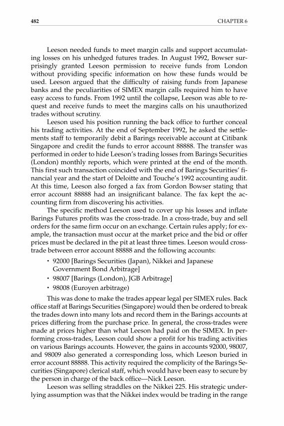
Leeson needed funds to meet margin calls and support accumulat-ing losses on his unhedged futures trades. In August 1992, Bowser sur-prisingly granted Leeson permission to receive funds from Londonwithout providing specific information on how these funds would beused. Leeson argued that the difficulty of raising funds from Japanesebanks and the peculiarities of SIMEX margin calls required him to haveeasy access to funds. From 1992 until the collapse, Leeson was able to re-quest and receive funds to meet the margins calls on his unauthorizedtrades without scrutiny.

Leeson used his position running the back office to further concealhis trading activities. At the end of September 1992, he asked the settle-ments staff to temporarily debit a Barings receivable account at CitibankSingapore and credit the funds to error account 88888. The transfer wasperformed in order to hide Leeson’s trading losses from Barings Securities(London) monthly reports, which were printed at the end of the month.This first such transaction coincided with the end of Barings Securities’ fi-nancial year and the start of Deloitte and Touche’s 1992 accounting audit.At this time, Leeson also forged a fax from Gordon Bowser stating thaterror account 88888 had an insignificant balance. The fax kept the ac-counting firm from discovering his activities.

The specific method Leeson used to cover up his losses and inflateBarings Futures profits was the cross-trade. In a cross-trade, buy and sellorders for the same firm occur on an exchange. Certain rules apply; for ex-ample, the transaction must occur at the market price and the bid or offerprices must be declared in the pit at least three times. Leeson would cross-trade between error account 88888 and the following accounts:

• 92000 [Barings Securities (Japan), Nikkei and JapaneseGovernment Bond Arbitrage]

• 98007 [Barings (London), JGB Arbitrage]• 98008 (Euroyen arbitrage)

This was done to make the trades appear legal per SIMEX rules. Backoffice staff at Barings Securities (Singapore) would then be ordered to breakthe trades down into many lots and record them in the Barings accounts atprices differing from the purchase price. In general, the cross-trades weremade at prices higher than what Leeson had paid on the SIMEX. In per-forming cross-trades, Leeson could show a profit for his trading activitieson various Barings accounts. However, the gains in accounts 92000, 98007,and 98009 also generated a corresponding loss, which Leeson buried inerror account 88888. This activity required the complicity of the Barings Se-curities (Singapore) clerical staff, which would have been easy to secure bythe person in charge of the back office—Nick Leeson.

Leeson was selling straddles on the Nikkei 225. His strategic under-lying assumption was that the Nikkei index would be trading in the range

482 CHAPTER 6


of 19,000 to 19,500. In this range he would rake in the money on the pre-miums of the sold options, while the calls and puts he sold would expireworthless. However, after the Kobe earthquake on January 17, 1995, theNikkei dropped to 18,950. At that point the straddle strategy was shaky.Leeson started to lose money on the puts, because the (short) value of theput options he sold was starting to overtake the (long) value of the premi-ums received from selling the puts and calls. Then he made a dangerousgamble; he believed that the market was overreacting and on January 20,three days after the earthquake, he bought 10,814 March 1995 futures con-tracts. On January 23, the Nikkei dropped 1,000 points to 17,950, and atthat point Leeson realized his gamble was a huge mistake. He was facingenormous losses from the long positions that he had just bought, alongwith unlimited losses on the puts.

In addition to selling straddles, Leeson’s reported arbitrage strategywas to go long or short the Nikkei 225 futures on the Osaka exchange,while simultaneously going the other direction on those same Nikkei 225futures on the SIMEX. This strategy would theoretically take advantage oftemporary mispricing differences of the same futures contract on two dif-ferent exchanges. Since these products were essentially identical (they de-rived all of their intrinsic value from the same underlying security), anylarge price differences between the Osaka and SIMEX Nikkei 225 March1995 futures contracts would be short-lived (or nonexistent) in an efficientmarket. This trading strategy is what Barings referred to as switching. Inreality, however, Leeson ignored the switching and was long the March1995 contract on both exchanges. Therefore, he was doubly exposed to theNikkei 225 instead of being hedged.

On January 20, the Osaka exchange lost 220 points and the SIMEXlost 195. If Leeson were short on the SIMEX, the net effect would havebeen (−220 + 195) = −25. However, he was long on both exchanges; there-fore, on January 20 he had a loss of (−220 − 195) = −415. During Januaryand February of 1995, Leeson suffered the huge losses that broke Barings.

6.6.2.1 How Leeson Hid the TradesIt is legal for an institution to separate a trade made on an exchange, as-suming that the trade is large and that its size might affect the marketprice of the position. This is done through “block transaction,” which ef-fectively splits the transaction into smaller transactions with differentcounterparts. Leeson traded this way within the Barings accounts (alsoknown as cross-trading). After the transactions, however, when he wassplitting the trades into the different accounts, he decided the price atwhich each trade should be recorded, and did not use the actual price ofthe trade. This is illegal. Although the sum of the small transactionmatches the overall trade, and the books were flat, Leeson was creditinggains to the Barings accounts and was offsetting them by recording losses

Case Studies 483


in the 88888 account. Since he was always losing money, he kept recordinglosses in this account, and was showing gains in the official books. Thisway Leeson fooled everybody at Barings and was able to show a prof-itable net position. Barings’ treasury never audited account 88888, whichmore accurately depicted Leeson’s true profits and losses. Account 88888was a ticking bomb that exploded in February 1995 and broke Barings.50

6.6.2.2 Leeson’s AssumptionsThe facts just discussed show the reasons behind Barings’ collapse. Whenreading them, one openly wonders what made Leeson so aggressive in thederivatives markets, why he thought he could profit from such aggressivetactics, and why he thought he could cover up his activities from his em-ployer. In every case involving huge derivative position losses, one usu-ally sees the “double-down” mentality take effect. In this case, Leesonsealed his fate the first day he decided to eschew the official Barings de-rivatives trading strategy. He was destined to eventually put himself in anet loss position due to the risky nature of the products he was trading.Once he did this, he had no other option but to keep doubling down in thehope that he could extricate himself from the situation. He could notmerely cap his losses and walk away, as that would mean he would haveto inform Barings management of his improper trading, and he surelywould have been fired by the firm at that point. That is why he did nothedge his positions once he started losing money. To do so might havesaved Barings from its eventual collapse, but it would not have beenenough to save his job. So, instead, he covered up his illicit trading prac-tices and kept raising the stakes. Leeson had been trading derivative prod-ucts improperly for some time prior to the disaster in early 1995. Becauseof his experience, albeit limited, with the Japanese equity markets, he feltconfident enough to take some rather large risk positions in early 1995.The Nikkei 225 index had been trading in a very tight range at the begin-ning of January 1995. Between January 4 and January 11, for example, theNikkei stayed between 19,500 and 19,700. With his double-long futuresposition on the SIMEX and OSE and his straddle options, Leeson was bet-ting that the Nikkei 225 index would increase or remain flat. If it stayedflat, he would collect the premiums from his sold put and call options andthese options would expire worthless. If the index increased greatly invalue, the premium from the sold put options would partially offset thelosing call option positions he sold, and he would more than make up forthis difference with the windfall profits from the double-long futures po-sitions on the SIMEX and OSE. Aside from his confidence in the volatilityand future direction of the Nikkei index, there is another reason Leesontook such a large market gamble. As the case details, Leeson was already£208 million in the hole as of the end of 1994.

484 CHAPTER 6


6.6.3 Effect

When a terrible earthquake rocked Japan on January 17, 1995, the Nikkeiplummeted. Many people explain Leeson’s last crazy behavior as evi-dence that he believed the Nikkei was still undervalued and had overre-acted to the disaster, and so continued to add to his futures positions.

Leeson had already built a large quantity of positions. Many peoplemay ask why he did not hedge those positions by building other positionsin his account. This is a good question, but Leeson’s dilemma was this: hestill believed prices would rise and his position would eventually breakeven or be profitable. However, even if he wanted to hedge those loss po-sitions, he could not do so. If he used the official accounts, which would bereported to Barings, he had to establish huge positions, and he didn’t be-lieve the price would crash deeper. Therefore, this strategy seemed toorisky. But he could not hedge in his internal 88888 account, either, becausein financial trading, a first-in-first-out rule is followed. Leeson’s hedgingposition was to liquidate all his Nikkei long and JGB and euroyen shortpositions. Thus, the floating loss became realized loss, and Leeson couldfind no place to recoup these huge losses. What he had to do was to keepthem and roll them over with floating loss (a nominal loss not booked yet).In this light, it is very easy to understand the later actions of Leeson. Hold-ing onto the belief that prices would rise, in order to protect his longNikkei futures, short JGB, and euroyen futures positions and in order tostop the crash of his short put options positions, Leeson executed his finalstrategy by placing huge amounts of orders to prop up the market.

Barings was on its way to collapse without realizing it due to a contin-uation of the deceptive practices that Leeson had engaged in since mid-1992. Between January 23 and January 27, 1996, he lost approximately$47,000,000 but was able to present a $55,000,000 profit to London by cross-trading between error account 88888 and Barings account 92000. The Lon-don office heard rumors that Barings was not able to meet its margin calls inAsia, but was not concerned because it felt this rumor was based on its longNikkei futures positions on the Osaka exchange, which were supposedlyhedged by corresponding short Nikkei futures position on the SIMEX. Afterall, Leeson’s official trading policy was to short Nikkei 225 futures onSIMEX to hedge Barings’ long positions on the Osaka exchange. However,he went long on Nikkei 225 futures, did not hedge these positions, and ex-posed Barings to significant risk. During January and February 1995, Leesonwas still able to receive funds from London to meet margin calls withoutbeing questioned. The payments forwarded to Singapore equaled $835 mil-lion, whereas Barings only had $615 million in capital. By late February theexposure in the Nikkei futures and options markets that Leeson created waslarger than Barings could handle. The enormity of the Nikkei 225 futuresmargin calls and the losses on the put options bankrupted Barings.

Case Studies 485



The collapse of Barings could have been avoided by:

• Making all Barings traders meet London International FinancialFutures Exchange (LIFFE) standards

• Managing account settlement and trading functions separatelyusing management information systems

• Exercising rigorous management oversight

6.6.4.1 Market RiskThe risks of Leeson’s strategy should be clear. If the market suffered asharp decline, Leeson would be exposed to tremendous potential losses.The premiums from the call options he sold would have been locked-inprofits, since these options would expire worthless in a sinking market.However, the put options he sold were increasing greatly in value as themarket declined. With strike prices between 18,500 and 20,000 on theNikkei 225 index, Leeson faced massive risk on these short put options ifthey became deep in the money. As the Nikkei plunged down under18,000 in mid-February 1995, that is exactly what happened. The losses onthese short options greatly exceeded the premiums gained on the expiredsold call options. Of course, Leeson’s double exposure to the March 1995Nikkei futures contract also left him open to the risks associated with thedeclining Japanese equity market. When he bought the additional 10,814contracts on January 20, he further increased this risk. Between January 20and February 15, the Nikkei dropped an additional 850 points. A decliningNikkei index was a large and obvious market risk that Leeson faced withhis derivatives book in early 1995. In addition to market risk, Leeson wasalso leaving himself exposed to event risk—the risk that something unex-pected and not directly related to the market could affect the market. Agreat example of event risk is the Kobe earthquake of January 17, 1995,which negatively impacted Leeson’s prospects for two reasons. First, ithelped send the Nikkei index into a tailspin. Second, the earthquakecaused increased volatility in these equity markets. Increased volatilityadds value to options, both calls and puts. As Leeson was short options atthis time, this increase in volatility further helped to destroy him. Theshort put options exploded in value as they became deeper in the moneyand as volatility increased.

6.6.4.2 Credit RiskBy late February, Barings’ exposure in the Nikkei futures and optionsmarkets was larger than the bank could handle. The enormity of theNikkei 225 futures margin calls and the losses on the put options bank-rupted Barings. Leeson created counterparty exposure for other institu-tions, which finally collapsed the bank.

486 CHAPTER 6


An appropriate management of counterparty risk and reporting ofspecific instrument exposures to counterparties would have been an addi-tional signal for management that some exposures were intolerable.

6.6.4.3 Operational RiskAs a result of Barings’ derivatives disaster, the market has attempted tohead off potential government regulation by improving industry self-regulation. New standards have been developed in accordance with theregulations created by the SEC, FSA, and other national regulators of de-rivatives sales practices, capital standards, and reporting requirements.Most, if not all, financial firms participating in derivatives have taken ahard second look at their control systems as a result of the Barings collapse.Indeed, some have wondered why a disaster such as this hadn’t happenedearlier. Valerie Thompson, an experienced trader at Salomon Brothers inLondon, claims that the deregulation of the British financial sector in the1980s created a vacuum that was filled by inexperienced traders in the1990s. Thompson observed that traders were created overnight withoutthe benefit of proper training because firms such as Barings were chasingmarkets previously dominated by the Americans and Japanese. This inex-perience contributed to Leeson’s undoing; he didn’t have the knowledge orexperience to admit his mistakes to upper management.51

Perhaps the collapse of Barings was an unfortunate, yet necessary,lesson that the market needed to learn. Graham Newall of BZW Futuresnotes that upper management now regularly inquires about activity in theomnibus account. Merrill Lynch Futures’ Tom Dugan notes that firms arefar less tolerant of individual stars these days and that everyone is held ac-countable for his or her actions. At the Futures Industry Association Ex-position in Chicago in October 1996, most industry experts agreed thattechnology is a key ingredient in preventing scams such as Leeson’s in thefuture. Risk management computer systems have been developed and im-proved as a result of Barings’ demise.52

Nick Leeson was obviously a man of questionable character, and thiswas evident before he was transferred to Barings Securities (Singapore). Hewas scheduled to appear in court due to the accumulation of unpaid debtand had already been taken to court and ruled against on another unpaiddebt charge. Leeson would not have been allowed to trade on the LIFFEdue to these problems, and therefore Barings should not have allowedhim to trade on the SIMEX. Making one person responsible for managingsettlements and the trading floor created a conflict of interest. Leeson wasable to use his influence in the back office to hide his actions on the trad-ing floor. Assigning one of these responsibilities to a different managerwould have kept Leeson from developing the ability to deceive the Lon-don office. Better management information systems were needed to en-sure that all account information was available at a central location and

Case Studies 487


that the complete status of all open accounts was known. Finally, Baringsmanagement should have monitored Leeson’s activities more proactively.Audits should have been performed more frequently and audit recom-mendations should have been immediately implemented or followed upon. Clearer lines of reporting should have been established, and office pol-itics should not have stood in the way of proper supervision.53

After analyzing Leeson’s trading and operations activities, the ques-tion arises as to what role and responsibility risk management had orcould have had. In general, three levels of risk management and valuationprocesses should be implemented by financial institutions: informationand risk reporting, risk control, and risk management.

Information and Risk ReportingThis is a basic process in measuring risk. The senior managers receive theinformation and reports showing risk created by trades and investments.The reporting side should provide complete, accurate, audited, and pre-cise professionally standard information. Risk reporting is essential invaluing and managing risk.

Leeson violated the principles of risk reporting. He secretly opened ac-count 88888 and sent false information to Barings from the time he arrived inSingapore. He controlled both the front and back offices at Barings Futures(Singapore), which meant he was both chief trader and head of settlements.Taking advantage of his excessive power, he suppressed the information inaccount 88888, made unauthorized trades, and manipulated profits.

The Barings risk reporting system was flawed. First, there was noone to supervise and assist Leeson in completing the reports and deliver-ing reliable information to his managers. Second, the managers never in-vestigated or doubted the credibility of Leeson’s trading activities asdetailed in his reports.

If the managers understood the nature of Leeson’s job, including ar-bitrage by taking advantage of the price differences between the SIMEXand the Tokyo Stock Exchange or the Osaka Securities Exchange, theywould have been suspicious of the unusual level of profits. Arbitragingthe price differences of futures contracts on separate exchanges entailsvery low risk. The fact that Leeson could make such a huge profit from al-most riskless trading is counter to fundamental modern financial theory,which states that low risk equals low return and high risk equals high re-turn. One question should have arisen: if such a low-risk and simple arbi-trage could yield such high returns, why did rival banks not execute thesame arbitraging strategy? In addition, as the volume of arbitraging trad-ing increases, the price differences tend to decrease, and therefore the potential profit from arbitrage also likely shrinks. Why could Leeson con-tinue arbitraging? Unfortunately no Barings executive recognized the ob-vious. Even when Leeson’s performance accounted for 20 percent of the

488 CHAPTER 6


entire firm’s 1993 profits and about half of its 1994 profits, no one tried todetermine where the enormous profits were coming from.

Risk ControlRisk control is used to set position limits for traders and business units toprevent individuals from having too much power. It can be used to mea-sure the risk in a variety of risky activities in diverse markets. Leeson con-tinued his unauthorized trading by taking advantage of his positions. Henever controlled the risk in his trading in Nikkei, JGB, and euroyen fu-tures as well as straddles in Nikkei options. He took extreme positionswithout hedging the risk and continued to execute a faulty strategy. Themarket exposure of his positions exceeded Barings’ total capital. In 1994,Barings transferred $354 million to Barings Futures (Singapore) for themargin call from the trading Leeson explained as risk-free arbitrage. It isastonishing that no one even asked Leeson to justify his requests.

Risk ManagementRisk management includes the analysis and measurement of positions andstrategies. It requires investment experience to supervise the exposures andthe persons taking the exposures. Barings had neither the risk controls northe risk measurement in place to analyze the exposure taken by Nick Lee-son, nor the analytical framework to monitor where the huge profits camefrom and what kinds of risks were being taken to generate the profits.

6.6.4.4 Systemic RiskThe systemic risks in the Barings case were substantial. However, all of theappropriate organizations moved to mitigate the problems created by thedebacle. The Singapore stock exchange reacted quickly on the same dayBarings was not able to cover the margin calls. The national banks pro-vided additional liquidity to ensure that the markets in London and Sin-gapore did not fall into a liquidity gap. The systemic risk was limited asthe loss for counterparty risk was limited to a one-day uncovered margincall, which was settled by Barings and later through ING Groep, which ac-quired the bankrupt Barings. The systemic risk was further contained bythe fact that Leeson’s speculation was not supported by an unheated mar-ket environment (such as in the months before the October 1987 crash) orthe turmoils around the ruble and the Russian bond crisis in August andSeptember 1998.

6.6.4.5 Additivity of Risk Management FrameworkThe regulatory, supervisory, and corporate governance framework failedcompletely in the Barings case. The key failures were by weak managerswho did not take responsibility for establishing systems and processesthat would have prevented the bankruptcy of Barings.

Case Studies 489


The capital adequacy framework should have required higher capi-tal to support the risk of Leeson’s trading strategy, as the strategy did notallow matching and offsetting of the transactions. The internal and exter-nal bank auditors should have realized the speculative background andinformed the appropriate supervisory authority.

6.7 NOTES

1. BBC News, “Business: The Economy Derivatives Firms Shut Down,”London: BBC News, Thursday, December 31, 1998.

2. Denise Lavoie, “Organized Criminal,” Associated Press and ABPnews.com,June 22, 1999; “Cendant to Pay $2.8 Billion Fraud Settlement,”APBnews.com, December 8, 1999, www.apbnews.com/safetycenter/business/1999/12/08/fraud1208_01.html; SEC press release, “FinancialReporting Case Filed Against Cendant,” Washington, DC: SEC, June 14,2000, www.sec.gov/news/press/2000-80-.txt.

3. “Three Bankers Brought Scandal to the Vatican,” Irish Times (August 29,1998); “The Old Man Who Hid Gold Under His Geraniums,” Irish Times(September 16, 1998).

4. For a discussion of knowledge of the market and the bank’s capacity, seeDavid Meerschwarn, Bankers Trust New York Corporation, Case Study 9-286-005, Cambridge, MA: Harvard Business School Press, 1985. For the legalcase between Procter & Gamble and Bankers Trust, see Procter & Gamble Co.v. Bankers Trust Co., 78 F. 3d 219 (6th Cir. 1996).

5. Senators John Kerry and Hand Brown, The BCCI Affair: A Report to theCommittee on Foreign Relations, 102d Congress, 2d Session, Senate Print 102-140, Washington, DC: Senate Printing Office, December 1992,www.fas.org/irp/congress/1992/1992_rpt/bcci/index.html; DavidMcKean, Why the News Media Took So Long to Focus on the Savings and Loanand BCCI Crisis, Evanston, IL: Northwestern University, AnnenbergWashington Program in Communications Policy Studies, 1993.

6. Deloitte & Touche: BRE-X Corporate Dissemination Services Inc.: The Deloitte &Touche Inc.’s Forensic Investigative Associate Inc. (FIA) Report to BRE-XMinderals, Deloitte & Touche, 1997.

7. Joseph Fitchett, “The Credit Lyonnais Debacle,” International HeraldTribune (London; October 3, 1996), p. 13; Ibrahim Warde, “Financiersflamboyants, contribuables brûlés,” Le Monde Diplomatique (July 1994),18–19.

8. Alan Greenspan, “Statement to Congress, U.S. Operations of Daiwa Bank,November 27, 1995,” Federal Reserve Bulletin (January 1996), 31–35; AlanGreenspan, “Statement to Congress: Issues Relating to the U.S. Operationsof Daiwa Bank, December 5, 1995,” Federal Reserve Bulletin (January 1996),133–138; Eugene A. Ludwig, Remarks by Eugene A. Ludwig, Comptroller of theCurrency, Before the Bank Administration Institute’s Asset/Liability and TreasuryManagement Conference, Release N6-119, Washington, DC: Office of the

490 CHAPTER 6


Comptroller of the Currency, October 22, 1996; Mari Yamaguchi, “ConvictedJapanese Trader Releases Memoir Accusing Daiwa of Cover-Up,” NewsTimes (January 7, 1997).

9. Matthew Fletcher, “Whom to Trust? Investors are Spooked by Scandal inAsia’s No. 1 Fund Manager,” Asiaweek (September 27, 1996),www.pathfinder.com/asiaweek/96/0927/bizl.html.

10. Tim Spofford, Lynch Street, Kent, OH: Kent State University Press, 1988.

11. IMRO, “IMRO Announces Morgan Grenfell Compensation,” Press Release37/96 (April 16, 1997), London; and IMRO, “IMRO Fines Morgan Grenfell£2,000,000 for Mismanagement of European Funds,” Press Release 05/97(April 16, 1997), London.

13. SFA, “SFA Disciplines NatWest and 2 Individuals,” press release, May 18,2000, www.fsa.gov.uk/sfa/press_releases/2000/sfa8-2000.html; commentsin “NatWest Fined for ‘Rogue Trader’ Loss,” This Is Money, May 18, 2000,www.thisismoney.com/20000518/nm15300.html; “SFO May ExamineNatWest,” Irish Times (July 31, 2001).

12. “The Big Noise from Columbus: The Journal of Finance Breaks the NASDAQScandal,” Investment Dealers Digest (May 22, 1995); Karen Donovan, “ThirdCircuit Reinstates Nasdaq Suit, Three Brokerage Firms Now Face SecuritiesClass Action,” National Law Journal (February 16, 1998), B01; In RE: NasdaqMarket-Makers Antitrust Litigation to: Consolidated Amended Complaint, M21-68(RWS), Civ. 3996 (RWS), M.D.L. No. 1023.

14. Sarkis Joseph Khoury, “It’s the Fundamentals: Stupid! The Orange CountyBankruptcy in Perspective,” working paper prepared for the BürgenstockConference, University of California Riverside, September 1995; PhilippeJorion, Value-At-Risk: The New Benchmark for Controlling Market Risk, NewYork: McGraw-Hill, 1997, p. 32; Philippe Jorion, “Philippe Jorion’s OrangeCounty Case: Using Value at Risk to Control Financial Risk,”www.gsm.uci.edu.

15. Anatoli Kuprianov, “Derivatives Debacles,” Economic Quarterly (FederalReserve Bank of Richmond) 81/4 (Fall 1995), 1.

16. Ibid.

17. Ibid.

18. Reto R. Gallati, Futures, Options, and Financial Risk Management, Case:Metallgesellschaft, Reading Package FE829, Boston, MA: Boston University,Fall 2000.

19. Allen B. Frankel and David E. Palmer, “The Management of Financial Risksat German Non-Financial Firms: The Case of Metallgesellschaft,”publication no. 560, New York: Board of Governors of the Federal ReserveSystem; August 1996.

20. Arthur Benson v. Metallgesellschaft Corp. et al., Civ. Act. No. JFM-94-484, U.S.District Court for the District of Maryland, 1994.

21. Anatoli Kuprianov, “Derivatives Debacles,” Economic Quarterly (FederalReserve Bank of Richmond) 81/4 (Fall 1995), 1.

Case Studies 491


22. “Metallgesellschaft: Germany’s Corporate Whodunit,” The Economist(London) 334/7900 (February 4, 1995), 71ff.

23. John Digenan, Dan Felson, Robert Kell, and Ann Wiemert:“Metallgesellschaft: A Case Study,” working paper, Illinois Institute ofTechnology, Stuart School of Business, Financial Markets and TradingProgram, undated.

24. Chicago Mercantile Exchange, Matching CME Quarterly Bankruptcy IndexFutures to Different Trading Horizons: A Primer, Chicago Mercantile Exchange,www.cme.com/qbi/qbiprimer.html.

25. “Metallgesellschaft: Germany’s Corporate Whodunit,” The Economist(London) 334/7900 (February 4, 1995), 71ff.

26. Charles Cathcart, “The Lessons of Metallgesellschaft,” Global Investor(London) 78 (December 1994–January 1995), 64.


28. Allen B. Frankel and David E. Palmer, “The Management of Financial Risksat German Non-Financial Firms: The Case of Metallgesellschaft,”publication no. 560, New York: Board of Governors of the Federal ReserveSystem; August 1996.


30. Jim Kharouf, “The Copper Trader Who Fell from Grace,” Futures (August1996).

31. Commodity Exchange Act, 7 U.S.C. §§ 6(a), 6(d), 9(a)(2).

32. Order Instituting Proceedings Pursuant to Sections 6(c) and 6(d) of theCommodity Exchange Act and Findings and Order Imposing Remedial Sanctions,Docket 98Civ. 4584(MP). Sumitomo was ordered to pay $125 million in civilpunitive sanctions and $25 million in restitution to market participantsharmed by the scheme.

33. Benjamin E. Kozinn, “The Great Copper Caper: Is Market ManipulationReally a Problem in the Wake of the Sumitomo Debacle?” Fordham LawReview (October 2000), 247.

34. Cargill v. Hardin, 452 F.2d 1154 (8th Cir., 1971).

35. Ibid., p. 1163.

36. Ibid.

37. Benjamin E. Kozinn, “The Great Copper Caper: Is Market ManipulationReally a Problem in the Wake of the Sumitomo Debacle?” Fordham LawReview (October 2000), 247.

38. Order Instituting Proceedings Pursuant to Sections 6(c) and 6(d) of theCommodity Exchange Act and Findings and Order Imposing Remedial Sanctions,Docket 98Civ. 4584(MP).

492 CHAPTER 6


39. Ibid.

40. Commodity Futures Trading Commission, Testimony of Brooksley Born,Chairperson, on Behalf of the Commodity Futures Trading Commission before theUnited States House of Representatives, Subcommittee on Capital Market,Securities and Government Sponsored Enterprises of the Committee on Bankingand Financial Services, Washington, DC: Commodity Futures TradingCommission, March 13, 1999.

41. U.S. Government, Hedge Funds, Leverage, and the Lessons of Long-Term CapitalManagement: Report of the President’s Working Group on Financial Markets,April, 1999, www.cftc.gov/tm/hedgefundreport.htm.

42. U.S. General Accounting Office, Long-Term Capital Management, RegulatorsNeed to Focus Greater Attention on Systemic Risk, October 1999.

43. “Long-Term Capital Management: Technical Note on a Global HedgeFund,” Thunderbird, American Graduate School of InternationalManagement, 1999.

44. Committee on the Global Financial System, A Review of Financial MarketEvents in Autumn 1998, October 1999.

45. Ibrahim Warde, “LTCM, a Hedge Fund Above Suspicion,” Le MondeDiplomatique (November 1998), English Internet edition, www.monde-diplomatique.fr/en/1998/11/05warde2.html, accessed August 24, 2000.

46. Philippe Jorion, “Risk Management Lessons from Long-Term CapitalManagement,” Working Paper Series (draft), University of California atIrvine, June 1999.

47. “How LTCM Came to the Edge of the Abyss,” Wall Street Journal (September11, 2000), pp. C1, C20.

48. Bank for International Settlement (BIS), Basel Committee on BankingSupervision, Highly Leveraged Institutions—Sound Practices, Basel,Switzerland: Bank for International Settlement, January 2000; Banks’Interaction with Highly Leveraged Institutions, Basel, Switzerland: Bank forInternational Settlement, January 1999.

49. Barry Hillenbrand, “The Barings Collapse: Spreading the Blame,” Time(London) 146/18 (October 30, 1995), www.time.com/time/magazine/archive/1995/951030/banking.box.html; Bank of England, The Bank ofEngland Report into the Collapse of Barings Bank, London: HMSO PublicationsCenter, 1995, www.numa.com/ref/barings/bar00.html.

50. Howard G. Chuan-Eoan, “Going For Broke,” Time 145/10 (March 13, 1995),18–25.

51. Ibid.

52. Jim Kharouf, Carla Cavaletti, and James T. Holder, “Top 40 Brokers,Technology Key to Stay Alive,” Futures (December 1996).

53. “Simex Criticizes Barings for Role in Leeson Debacle,” Herald Tribune (March16, 1995), p. 1; “Barings Abyss,” Futures 26/5 (May 1995), 68–74; “BoE ReportDetails Barings’ Guiles, Goofs,” Futures 26/10 (September 1995), 68–74.

Case Studies 493


G L O S S A R Y

ABS See asset-backed security.

absolute return Measure of net economic return. Takes into account all costs (for example,cost of funding, balance sheet charges, and administrative expenses).accrual (Z) bond A long-term, deferred-interest CMO bond that distributes no interest (in-terest is capitalized) until certain other bonds have been retired.accumulation plan An investment plan under which an investor may regularly buy speci-fied minimum amounts of investment company shares. Dividends and distributions are usu-ally reinvested automatically. Sometimes referred to as a systematic plan. (See contractualplan.)accumulation unit The basic valuation unit of a deferred variable annuity. Such units arevalued daily to reflect investment performance and the prorated daily deduction for ex-penses.adjustable-rate mortgage (ARM) A mortgage that permits the lender to adjust its interestrate periodically on the basis of movement in a specified index. Also used collectively to referto ARMs and graduated-payment adjustable-rate mortgages (GPARMs).ADR See American Depositary Receipt.

American Depositary Receipt (ADR) A certificate issued by an American bank as evi-dence of ownership of foreign shares. The certificate is transferable and can be traded. Theoriginal foreign stock certificate is deposited with a foreign branch or correspondent bank ofthe issuing American bank.amortization Gradual reduction of mortgage debt through periodic payments scheduledover the mortgage term.annuity contract A contract issued by an insurance company that provides payments for aspecified period, such as for a specified number of years, or for life. (See variable annuity.)arbitrage The simultaneous purchase and sale of the same (or equivalent or related) secu-rities to take advantage of price differences prevailing in separate markets. Pure arbitrage in-volves trading the same instruments for different prices at the same time.ARCH See autoregressive conditional heteroskedascticity.

ARM See adjustable-rate mortgage.

arm’s-length transaction A transaction that is conducted as though the parties were unre-lated, thus avoiding any semblance of conflict of interest.ask price A potential seller’s lowest declared price for a security.asset-backed security (ABS) Bonds or debt securities collateralized by the cash flow froma pool of auto loans, credit card receivables, vehicle and equipment leases, consumer loans,and other obligations.asset liability management Matching the level of debt and amount of assets. Financial in-stitutions carry out asset liability management when they match the maturity of their de-posits with the length of their loan commitments to keep from being adversely affected byrapid changes in market prices.at the money When the strike price of an option is the same as the price of the underlyinginstrument.

495

Gallati_gloss_1p_j.qxd 2/27/03 9:16 AM Page 495


at-the-money forward When the strike price of an option is the same as the forward priceof the underlying instrument.autocorrelation Serial correlation in which observations on the same time series are corre-lated over time. In mathematical terms, the covariance between data recorded sequentiallyon the same series is nonzero.autoregressive conditional heteroskedascticity (ARCH) A time-series process that mod-els volatility as dependent on past returns.

back-office operations Clerical operations at trading institutions that include confirmationand settlement of trades, record keeping, and regulatory compliance.backtesting A method of testing the validity of VaR models, usually performed by com-paring risk forecasts with actual or hypothetical trading results.balanced fund An investment company that invests in varying proportions from time totime in equity and fixed-income securities for growth and income.balance-sheet capital The amount of capital reported under generally accepted accountingprinciples.Bank for International Settlement (BIS) An agency headquartered in Basel, Switzerland,that serves as an international forum for monetary cooperation and banking regulation.banker’s acceptance A time or sight draft drawn on a commercial bank by a borrower, usu-ally in connection with a commercial transaction.base currency Currency in which operating gains and losses are measured. Typically this isthe reporting currency of a company.basis The difference between a futures contract price for an item and the current spot priceof the same item.basis risk The potential loss due to small pricing differences between equivalent instru-ments, such as futures, bonds, and swaps. Hedges are often subject to basis risk.Basel regulatory market risk capital requirements Minimum requirements for capital thatinternational banks must carry to cushion against adverse market movements.benchmark A custom or published index of a predetermined set of securities used to com-pare performance and risk. Asset managers’ performance is often gauged against a bench-mark of published market indexes.benchmarking Comparing information about one entity to like information of another en-tity or composite group for the purpose of determining areas for potential improvement andto identify best practices.benchmark yield curves Derived yield curves that correspond to a country, industry, orcredit rating category; typically generated through a yield-curve-fitting algorithm.beta (b) A volatility measure relating the rate of return on a security to the return of its mar-ket over time. It is defined as the covariance between a security’s return and the return on themarket portfolio divided by the variance of the return on the market portfolio.bid price The highest declared price a potential buyer is willing to pay for a security at aparticular time.binomial distribution The distribution of a data set for which there are only two possibleoutcomes (success and failure).BIS See Bank for International Settlement.

Black-Scholes A model invented by Fischer Black and Myron Scholes for pricing call op-tions based on arbitrage arguments. Key variables are current asset price, exercise price, risk-free rate, time to expiry, and expected standard deviation of the asset.

496 Glossary


bond discount The difference between the face amount of a bond and the lower price paidby the buyer.bond premium The difference between the face amount of a bond and the higher pricepaid by a buyer.bonds Debt instruments issued with a maturity greater than one year. The purchase of abond is comparable to making a loan.book shares Investment company shares whose ownership is evidenced by records main-tained by a transfer agent rather than by physical stock certificates.break point The volume at which a quantity of securities qualifies for a lower sales chargewhen purchased. Also, an aggregate amount of investment company assets in excess ofwhich a lower investment advisory fee is rate charged.broker An agent, often a member of a stock exchange firm or an exchange member, whoexecutes orders to buy or sell securities or commodities and charges a commission. [See Sec-tion 2(a)(6) of the Investment Company Act of 1940.]bunching Grouping transactions in the same security for several investment clients of thesame investment advisor to obtain the benefit of lower commission changes or other trans-action costs.

calendar spread Options strategy that entails buying two options on the same securitywith different maturities. If the exercise prices are the same, it is a horizontal spread. If the ex-ercise prices are different, it is a diagonal spread.

call option A contract that entitles the holder to buy (call), at the holder’s option, a speci-fied number of units of a particular security at a specified price at any time until the statedexpiration date of the contract. The option generally applies to round lots of securities.cap An option contract that protects the holder from a rise in interest rates, or some otherunderlying fundamental, beyond a certain point.capital asset pricing model (CAPM) A model which relates the expected return on an assetto the expected return on the market portfolio.CAPM See capital asset pricing model.

caps and floors Interest-rate options. Caps are an upper limit on interest rates (if you buy acap, you make money if interest rates move above the cap strike level). Floors are a lowerlimit on interest rates (if you buy a floor, you make money if interest rates move below thefloor strike level).cash-flow map A report that shows net cash flows of foreign-exchange- and interest-rate-related cash flows (typically grouped by maturity, country, or credit rating).cash flow at risk Estimated potential cash-flow loss (through reduction in revenues or in-crease in outgoings) due to adverse market movements (for example, unfavorable move-ments in interest rates, exchange rates, commodity prices, and other markets) within aspecific time horizon and subject to a given confidence level.CBOE See Chicago Board Options Exchange.

CD See certificate of deposit.

certificate of deposit (CD) Generally, short-term, interest-bearing, negotiable certificatesissued by commercial banks or by savings and loan associations against funds depositedwith the issuing institution.change return See log return.

Chicago Board Options Exchange (CBOE) A national securities exchange, based inChicago, that provides a continuous market for trading in derivatives. Various other ex-

Glossary 497


changes, such as the American, Pacific, Philadelphia, and Baltimore and Washington Ex-changes, also provide such markets.churning A process of executing unnecessary portfolio securities transactions to generatecommissions.clearing agency A central location at which members’ security transactions are matched todetermine the minimum quantities to be received or delivered.clearing risk The possibility that an institution may not be reimbursed on the same valuedate for payments made on behalf of customers.closed-form solution A solution is closed form when an exact solution can be found for aprecise mathematical representation of the problem. Otherwise, it is considered an open-form solution.

closed-end investment company A mutual fund having a fixed number of shares out-standing, which it does not stand ready to redeem. Its shares are traded similarly to those ofother public corporations. [See Section 5(a) of the Investment Company Act of 1940.]closed-up fund An open-end investment company that no longer offers its shares for saleto the general public but still stands ready to redeem its outstanding shares.close-out netting An arrangement to settle with one single payment all contracted but notyet due liabilities to and claims on an institution, immediately upon the occurrence of one ofa list of defined events, such as the appointment of a liquidator to that institution. (See net-ting by novation and obligation netting).CMO See collateralized mortgage obligation.

collar Combination of a cap and a floor that protects the buyer within a band of interestrates.collateralized mortgage obligation (CMO) Mortgage-backed bond secured by the cashflow of a pool of mortgages.commercial paper (CP) Short-term, unsecured, promissory notes issued by corporations.Commercial paper is usually sold on a discount basis. [See Section 3(a)(3) of the SecuritiesAct of 1933 and Section 3(a)(10) of the Securities Exchange Act of 1934.]compliance risk The risk arising from violations or nonconformance with laws, rules, reg-ulations, prescribed practices, or ethical standards.confidence bands Projected upper and lower boundaries for portfolio returns (e.g., 5 per-cent band breaks are associated with a 95 percent confidence band).confidence interval A range of the possible values of a population, usually centeredaround the mean.confidence level A specified level of certainty for a statistical prediction (e.g., 95 percentconfidence worst-case loss).confidence level scaling factor A multiplier to scale standard deviation to a specified con-fidence level, assuming normality (e.g., 1.65 is the confidence level scaling factor to arrive ata 95 percent one-tailed confidence level).contango An interest factor reflecting the excess of the future price of a commodity contractover the spot price.contingent lending risk The risk that potential obligations will become actual obligationsand will not be repaid on time. Contingent lending risk occurs in products ranging from let-ters of credit and guarantees to unused loan commitments.control Defined by Section 2(a)(9) of the Investment Company Act of 1940 as the power toexercise (whether exercised or not) a controlling influence over the management of policiesof a company, unless that power results solely from an official position with the company.conventional mortgage A mortgage that is not insured or guaranteed by the federal gov-ernment.

498 Glossary


convertible bond A bond with an embedded option that allows the holder to convert thebond to common stock.convertible securities Securities carrying the right (either unqualified or under stated con-ditions) to exchange the security for other securities of the issuer or of another issuer.convexity An upward-bowing shape of a security’s payoff pattern. In technical parlance, itmeans that the second derivative of value with respect to some variable is positive.correlation (ρ) A linear statistical measure of the comovement between two random vari-ables. A correlation ρ (Greek letter rho) ranges from +1.0 to −1.0. Observing clumps of firmsdefaulting together geographically or by industry is an example of positive correlation of de-fault events.counterparty The partner in a credit facility or transaction in which each side takes broadlycomparable credit risk. When a bank lends a company money, the borrower (not the coun-terparty) has no meaningful credit risk to the bank. When the same two agree on an at-the-money forward exchange contract or swap, the company is at risk if the bank fails, just asmuch as the bank is at risk if the counterparty fails (although for the opposite movement inexchange or interest rates). After inception, swap positions often move in or out of themoney, and the relative credit risk changes accordingly.country risk A broad risk category encompassing political risk and transfer risk (alsoknown as cross-border risk).coupon stripping The separation of interest coupons from the corpus of a bearer bond.covariance (cov) The variability of a portfolio of data sets.covenants Legal restrictions placed on an organization, often tied to debt issues.CP See commercial paper.

credit (debt) rating A process of ranking obligations (facilities) and, at some banks, obli-gors (borrowers) according to their relative risk. Moody’s and S&P assign both short- andlong-term ratings to individual issues of a borrower. Country ratings are also provided.credit exposure The amount subject to a change in value upon a change in credit qualitythrough either a market-based revaluation in the event of an upgrade or downgrade, or theapplication of a recovery fraction in the event of default.credit quality Generally refers to an obligor’s relative chance of default, usually expressedin alphabetic terms (e.g., Aaa, Aa, A).credit-rating methodology Credit ratings are assigned to assess counterparty risk. Creditratings essentially rank counterparties according to risk of default, risk of loss, or both. Thereare many forms and many approaches.credit risk/exposure The risk that a counterparty will not settle a contractual obligation forfull value as defined and on time, either when due or at any time thereafter. In exchange-for-value systems, the risk is generally defined to include replacement risk and principal risk.credit scoring A method of using scorecards to predict an expected default rate. Applicantsare ranked according to an expected default rate for each score. Both behavioral scores andapplication data can be used for new applicants.credit spreads A spread over government rates to compensate investors for credit risk, typ-ically expressed in basis points (0.01 percent).cross-currency settlement risk See foreign-exchange settlement risk.

currency risk The risk that a change in the value of a foreign currency will affect the valueof an asset, liability, or financial instrument that is denominated in the foreign currency.current exposure For market-driven instruments, the amount it would cost to replace atransaction today should a counterparty default. If there is an enforceable netting agreementwith the counterparty, the current exposure would be the net replacement cost; otherwise, itwould be the gross amount.

Glossary 499


custodian A bank, trust company, or, less frequently, a member of a national securities ex-change, responsible for receiving delivery and for the safekeeping of an investment com-pany’s cash and securities. [See Section 17(f) of the Investment Company Act of 1940.]custody arrangements Arrangements under which the trustee’s only responsibilities are toensure the safekeeping of assets and to follow the instructions of approved individuals as setout in the trust agreement.

daily earnings at risk (DEaR) The estimated potential loss of a portfolio’s value resultingfrom an adverse move in market factors over a specific time horizon. Measures the maxi-mum estimated losses on a given position that can be expected to be incurred over a singleday, with 95 percent confidence.daily limits Limits established by exchanges on fluctuations in prices of futures contracts(other than contracts for delivery in the current month) during a trading session.dealer A person or firm acting as a principal rather than as an agent in buying and sellingsecurities. Mutual fund shares are usually sold through dealers. [See Section 2(a)(11) of theInvestment Company Act of 1940.]DEaR See daily earnings at risk.

decay factor (l) The weight λ (Greek letter lambda) applied in the exponential moving av-erage. It takes a value between 0 and 1. In RiskMetrics, λ is 0.94 in the calculation of volatili-ties and correlations for a 1-day horizon and 0.97 for a 1-month horizon.delayed delivery contract A transaction in which delivery and payment are delayed longerthan in normal transactions.delivery versus payment (DVP) A mechanism in an exchange-for-value settlement systemthat ensures that the final transfer of one asset occurs if and only if the final transfer of otherassets occurs. Assets could include monetary assets (such as foreign exchange), securities, orother financial instruments. (See payment versus payment.)delta (d) The change in a derivative’s price in relation to a given and incremental change inthe price of the underlying instrument. For example, a delta of −0.5 would imply a −1⁄2 per-cent change in the derivative’s price given a 1 percent increase in the underlying asset. (Seevolatility.)derivative A financial instrument that derives its value from the value and characteristicsof another underlying asset, index, or reference rate, called the underlying instrument.

diffusion process Process that assumes continuous (as opposed to discrete) price changesof asset prices.disclosure risk Risk that occurs when acting as an agent for other investors, as an under-writer, or as an advisor on a transaction.discount The amount of points collected from the mortgagor. The purpose of a discount isto adjust the yield upward above the note rate.diversification The process of risk reduction achieved by assembling a portfolio of securi-ties with correlations less than 1.dividends Prorated payments to shareholders from net investment income and realizedcapital gains.duration (Macaulay) See Macaulay duration.

DVP See delivery versus payment.

EaR See earnings at risk.

earnings at risk (EaR) The amount of earnings that are at risk over a defined period oftime; for example, the earnings that could be claimed by loss over a 10-day time frame by a

500 Glossary


2-standard-deviation event. Similar to cash flow at risk, except for necessary adjustmentsdue to accounting treatments of cash flows when determining earnings. Typical adjustmentsinclude deferral of cash flows that are subject to deferral accounting treatment, advancetreatment of cash flows that are accounted accrually, and inclusion of operating cash flowsthat are hedged.economic capital An equity reserve or cushion for unexpected losses. It ensures that a com-pany remains solvent and stays in business even under extreme conditions. It is important torecognize that economic capital is distinct from regulatory capital, which focuses on marketand credit risk. Conceptually, economic capital is comprehensive and covers all significantrisks.economic exposures Market exposures that consider how changes in foreign-exchangerates, interest rates, or commodity prices can affect the overall operating environment of afirm (for example, level of demand for products and services). Also called strategic exposures.

EDF See expected default frequency.

Employee Retirement Income Security Act (ERISA) A federal law enacted in 1974 that setinvestment guidelines for management of private pension plans and profit sharing plans, in-cluding employee vesting and conduct of plan administrators.enterprise risk The risk of loss associated with the occurrence of firmwide events, such asthe loss of key personnel, the loss of important customers, or the risk of litigation. Some ofthese risks are insurable; some can be actively managed to mitigate their impact.equity risk Risk that occurs when an institution invests in, holds, or receives equity, equity-like securities, or other junior securities in nonaffiliated entities. These securities include in-struments such as common shares, preferred shares, and related derivative instruments.equity securities Common and preferred stocks and debentures convertible into commonstocks.ERISA See Employee Retirement Security Act.

eurodollars U.S. dollars deposited in banks outside the United States.event risk The risk associated with the occurrence of a single event, such as the default onan individual loan, a failure to process an item accurately, or an act of fraud.excess returns Returns above the benchmark rate.excessions Confidence-level band breaks (i.e., observed exceptions or outliers).ex-dividend A security that no longer carries the right to the most recently declared divi-dend; or the period of time between the announcement of the dividend and the payment. Asecurity becomes ex-dividend on the ex-dividend date (set by the the NASD), which is usu-ally two business days before the record date (set by the company issuing the dividend). Fortransactions during the ex-dividend period, the seller, not the buyer, will receive the divi-dend. Ex-dividend is usually indicated in newspapers with an x next to the stock or mutualfund’s name. In general, a stock price drops the day the ex-dividend period starts, since thebuyer will not receive the benefit of the dividend payout till the next dividend date. As thestock gets closer to the next dividend date, the price may gradually rise in anticipation of the dividend.expected default frequency (EDF) The statistically derived likelihood that any given in-strument will go into default.exponential moving average Method of applying weights to a set of data points with theweights declining exponentially over time. In a time series context, this results in weightingrecent data more than data from the distant past.ex-rights Similar to ex-dividends. The buyer of a stock selling ex-rights is not entitled to arights distribution.ex-warrants Stocks or bonds trading without attached warrants, entitling holders to sub-scribe to additional shares within specified periods and at specified prices.

Glossary 501


failure to deliver Securities that the selling broker or other financial institution has not de-livered to the buyer at the settlement or clearance date.failure to receive Securities that the buying broker or a financial institution has not re-ceived from the seller at the settlement or clearance date.fair value An estimated value for securities and assets determined in good faith by theboard of directors under the Investment Company Act of 1940, and which has no readilyavailable market quotation. [See Section 2(a)(41).]fat tails See leptokurtosis.

fiduciary risk Risk that occurs when an institution is charged with the responsibility of act-ing as a trustee for third parties. The risk is greatest when placed in this position involuntar-ily—that is, without having a trust agreement in place that defines the restrictions.fiduciary services Services involving entrusting assets owned by one party to another party.final, finality Irrevocable and unconditional.final settlement Settlement that is irrevocable and unconditional. (See settlement.)fixed income Refers to interest rate instruments (e.g., bonds, zero-coupon bonds, and floating-rate notes). A preferred stock or debt security with a stated percentage or dollar in-come return.fixed-rate mortgage A mortgage that provides for only one interest rate for the entire termof the mortgage. If the interest rate changes because of enforcement of the due-on-sale pro-vision, the mortgage is still considered a fixed-rate mortgage.flat A method of trading in certain types of bonds, usually income bonds that do not payinterest unless it has been earned and declared payable, or bonds on which the issuing cor-poration has defaulted in paying interest.floater A debt instrument with a variable coupon, paying a rate indexed to a money mar-ket rate.floor An option contract that protects the holder against a decline in interest rates or someunderlying instrument below a certain point.foreclosure The legal process by which a borrower in default under a mortgage is deprivedof the interest in the mortgaged property.Foreign exchange (FX) risk Risk of loss due to movements in foreign-exchange rates.foreign-exchange settlement exposure The amount at risk when a foreign-exchange trans-action is settled. This equals the full amount of the currency purchased. The exposure lastsfrom the time that a payment instruction for the currency sold can no longer be cancelledunilaterally until the time the currency purchased is received with finality. (See creditrisk/exposure and foreign-exchange settlement risk.)foreign-exchange settlement risk The risk that one party to a foreign-exchange transactionwill pay the currency it sold but not receive the currency it bought. This is also called cross-currency settlement risk or principal risk.

forward A contract obligating one party to buy, and the other to sell, a specific asset for afixed price at a future date.forward exchange contract An agreement to exchange the currencies of different countriesat a specified future date at a specified rate (the forward rate). Unlike a securities futures con-tract, the terms of a forward contract are not standardized.forward pricing The pricing of mutual fund shares for sale, repurchase, or redemption at aprice computed after an order has been received. Mutual fund shares are usually priced onceor twice a day.forward rate agreement (FRA) An agreement to exchange dollar amounts at a specified fu-ture date based on the difference between a particular interest-rate index and an agreed fixedrate.

502 Glossary


front running Buying or selling securities for an institution in advance of executing a cus-tomer’s transaction.fundamental rating models These are typically proprietary models which have been builtby individual banks or vendors. They, too, try to predict EDRs; however, they allow chang-ing the firm’s balance sheet, stress-testing cash flows, etc. in order to develop an EDR.futures Contracts covering the sale of financial instruments or physical commodities forfuture delivery on an exchange. A forward contract that is standardized and traded on an ex-change.futures contract A transferable agreement to deliver or receive during a specific futuremonth a standardized minimum grade or a financial instrument of standardized specifica-tion under terms and conditions established by the designated contract market.FX risk See foreign-exchange risk.

gamma (g) The ratio of an option’s change in delta relative to an incremental change in theprice of underlying asset. It is a measure of the rate of change of a security’s delta.GPARM Graduated-payment adjustable-rate mortgage. (See adjustable-rate mortgage.)growth fund An investment company investing primarily or entirely in growth-industrysecurities, emphasizing future capital appreciation over current yield.growth stock The stock of a company whose earnings are expected to increase, thus raisingthe market value of the stock. Growth-stock companies generally reinvest a substantialamount of their earnings rather than paying them out in cash dividends.

hedge Transaction that is designed to reduce the risk of a position or a portfolio by takinga corresponding offsetting position. Hedges are good at eliminating market risk, but oftenresult in basis risk.hedge fund An investment company seeking to minimize market risks by holding securi-ties believed likely to increase in value while simultaneously taking short positions in secu-rities believed likely to decrease in value. The only objective is capital appreciation.hedging A means of risk protection against extensive loss due to adverse price fluctuationsby buying or selling a futures contract or option to offset a present or anticipated position ortransaction in the cash market.historical simulation A nonparametric method of using past data to make inferences aboutthe future. One application of this technique is to take today’s portfolio and revalue it usinghistorical price and rate data.holding period The amount of time that it is assumed that a financial instrument will be re-tained. The time period over which the risk measurement should apply.hot spot A measure of contribution to portfolio risk, highlighting significant risk concen-tration. A trademark of Goldman Sachs.

implied volatility An indication of volatility obtained from observable prices for tradedoptions, and which captures the market’s current expectations for the future distribution ofmarket prices.incentive compensation A fee paid to an investment company’s advisor that generallyconsists of a basic fee plus a bonus (or less a penalty) if the fund’s performance exceeds (orfails to match) that of a specified stock index.incremental VaR A measure of a position’s impact on VaR as the position size increases.

Glossary 503


independent Implies no correlation or relationship between variables.individual incentive Objective-based or commission-type incentive, individualized to applyto technicians, professionals, managers, and individual contributors.information risk Risk arising from lack of sufficient and or timely information, particu-larly in light of changing economic or market conditions.International Swap Dealers Association (ISDA) A committee sponsored by this organiza-tion was instrumental in drafting an industry standard under which securities dealers wouldtrade swaps. Included in this was a draft of a master agreement by which institutions wouldoutline their rights to net multiple offsetting exposures which they might have to a counter-party at the time of a default.integrated risk The risk that concentrations and/or interrelationships between risks (i.e.,credit and market risk) are not recognized.interest margin deposit A commodity transaction term for the amount of money or itsequivalent, specified by the commodity exchange under which the contract is traded, that isheld as a good-faith deposit to ensure that the customer meets the variation margin require-ment.interest method A method of amortizing discount or premium on debt that results in aconstant rate of interest on the sum of the face amount of debt and the unamortized premiumor discount at the beginning of each period.interest-rate risk The risk to earnings or capital arising from movements in interest rates.Interest-rate risk arises usually from shift, twist, and butterfly factors; from differences be-tween the timing of rate changes and the timing of cash flows (repricing risk); and fromchanging rate relationships among different yields.interest-rate swap A binding agreement between counterparties to exchange periodic in-terest payments on a predetermined notional principal amount. For example, one party willpay fixed and receive variable interest rate on a $100 million notional principal amount.internal models approach A proposal by the Basel Committee that permits banks to useapproved risk models to calculate market risk capital.internal rate of return (IRR) The interest rate that, when used as a discount rate, equatesthe price of a financial instrument to its individual discounted cash flows.International Organization of Securities Commissions (IOSCO) A committee of supervi-sory authorities for securities firms in major industrialized countries.Internet An uncontrolled (not governed, not owned) network of computers linked to oneanother that provides consistent pathways for communication.in the money When an option has positive intrinsic value (that is, for a call option, whenthe price is above the strike, and for a put option, when the price is below the strike).inverse floater A mortgage-backed bond, usually part of a CMO, bearing an interest ratethat declines as an index rate increases, and vice versa.investment advisor (manager) Under Section 2(a)(20) of the Investment Company Act of1940, a company providing investment advice, research, and often administrative and simi-lar services for a contractually agreed-on fee, generally based on a percentage of net assets.Investment Advisory Act of 1940 A law requiring investment advisors and firms provid-ing investment advice to register with the SEC and adhere to SEC regulations.investment advisory agreement An agreement between an investment company and aninvestment manager, engaging the investment manager to provide investment advice to theinvestment company for a fee. [See Sections 15(a), 15(c), and 36(b) of the Investment Com-pany Act of 1940.]investment company A company, as defined in Section 3(a) of the Investment CompanyAct of 1940, that primarily invests, reinvests, or trades in securities [Section 3(a)(1)], issues

504 Glossary


face-amount certificates [Section 3(a)(2)], or is engaged in investing and owning investmentsecurities.Investment Company Act of 1940 A set of federal laws enforced by the SEC that regulatethe registration and activities of investment companies.investment manager A manager of a portfolio of investments.IOSCO See International Organization of Securities Commissions.

IRR See internal rate of return.

ISDA See International Swap Dealers Association.issuer risk The risk that the market value of a security or other debt instrument maychange when the perceived or actual credit standing of the issuer changes.

kurtosis (K) Characterization of the relative peakedness or flatness of a distribution whencompared to a normal distribution.

lambda (l) See decay factor.

legal and regulatory risk Risk that occurs whenever a bank, a related corporate entity(such as a nonbank subsidiary or affiliate), a transaction, or a customer is subject to a changein exposure resulting from regulatory, civil, or criminal sanctions or litigation. The risk that acountry’s laws will make certain derivative contracts unenforceable.leptokurtosis Characterization of the thickness of the tails of a distribution compared tothe normal distribution; often called fat tails. The situation in which there are more occur-rences far from the mean than predicted by a standard normal distribution.leverage Upside opportunity; amount available to earn as incentive compensation. Alsodefined as the ratio of equity to loan capital.LIED See loss in event of default.

linear derivative Derivative security whose value changes proportionally with changes inunderlying rates. Examples of common linear derivatives are futures, forwards, and swaps.linear function A payoff pattern that follows a straight line. Any given change in the valueof a factor will have the same impact on the price, regardless of the level of the factor.linear risk For a given portfolio, when the underlying prices or rates change, the incremen-tal change in the payoff of the portfolio remains constant for all values of the underlyingprices or rates. When the payoff of the portfolio is not constant, the risk is said to be nonlinear.

liquidity At the enterprise level, the ability to meet current liabilities as they fall due; oftenmeasured as the ratio of current assets to current liabilities. At the security level, the ability totrade in volume without directly moving the market price; often measured as bid–ask spreadand daily turnover.liquidity risk The risk that a counterparty (or participant in a settlement system) will notsettle an obligation for full value when due. Liquidity risk does not imply that a counterpartyor participant is insolvent, because the counterparty or participant may be able to settle therequired debit obligations at some later time.listed security A security listed and traded on a stock exchange.loan-equivalent risk The risk exposure of a transaction can be converted into one quantity,as if the transaction were a loan of a certain magnitude with specific risks assigned to it.lognormal distribution Distribution in which the natural logarithms of the data elementsare normally distributed.log return The continuously compounded rate of return is assumed to be normally distrib-uted. If we call this rate r and we call the effective annual rate re, then re = er − 1, and because

Glossary 505


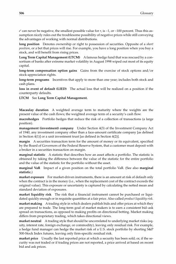
er can never be negative, the smallest possible value for re is −1, or −100 percent. Thus this as-sumption nicely rules out the troublesome possibility of negative prices while still conveyingthe advantages of working with normal distributions.long position Denotes ownership or right to possession of securities. Opposite of a shortposition, or a bet that prices will rise. For example, you have a long position when you buy astock, and will benefit from rising prices.Long Term Capital Management (LTCM) A famous hedge fund that was rescued by a con-sortium of banks after extreme market volatility in August 1998 wiped out most of its equitycapital.long-term compensation option gains Gains from the exercise of stock options and/orstock-appreciation rights.long-term programs Incentives that apply to more than one year; includes both stock andcash plans.loss in event of default (LIED) The actual loss that will be realized on a position if thecounterparty defaults.LTCM See Long Term Capital Management.

Macaulay duration A weighted average term to maturity where the weights are thepresent value of the cash flows; the weighted average term of a security’s cash flow.macrohedges Portfolio hedges that reduce the risk of a collection of transactions (a largeposition).management (investment) company Under Section 4(3) of the Investment Company Actof 1940, any investment company other than a face-amount certificate company [as definedin Section 4(1)] or a unit investment trust [as defined in Section 4(2)].margin A securities transaction term for the amount of money or its equivalent, specifiedby the Board of Governors of the Federal Reserve System, that a customer must deposit witha broker in a securities transaction on margin.marginal statistic A statistic that describes how an asset affects a portfolio. The statistic isobtained by taking the difference between the value of the statistic for the entire portfolioand the value of the statistic for the portfolio without the asset.marginal VaR Impact of a given position on the total portfolio VaR. (See also marginal statistic.)market exposure For market-driven instruments, there is an amount at risk of default onlywhen the contract is in the money (i.e., when the replacement cost of the contract exceeds theoriginal value). This exposure or uncertainty is captured by calculating the netted mean andstandard deviation of exposures.market liquidity risk The risk that a financial instrument cannot be purchased or liqui-dated quickly enough or in requisite quantities at a fair price. Also called product liquidity risk.

market making A trading style in which dealers publish bids and offer prices at which theyare prepared to trade. The long-term goal of market makers is to earn a consistent bid–askspread on transactions, as opposed to making profits on directional betting. Market makingdiffers from proprietary trading, which takes directional views.market neutral A trading style that should be uncorrelated to underlying market risks (eq-uity, interest rate, foreign exchange, or commodity), leaving only residual risk. For example,a hedge fund manager can hedge the market risk of a U.S. stock portfolio by shorting S&P500-Stock Index futures, leaving only firm-specific residual risk.market price Usually the last reported price at which a security has been sold; or, if the se-curity was not traded or if trading prices are not reported, a price arrived at based on recentbid and ask prices.

506 Glossary


market rates Interest rates, equity prices, commodities prices, foreign-exchange rates,credit spreads, futures prices, and other market-related prices or levels.market risk The risk that changes in market prices and conditions will adversely affect thebook or market value of on- or off-balance-sheet positions by movements in equity and interest-rate markets, currency-exchange rates, and commodity prices.market risk capital requirement The minimum amount of capital needed to support mar-ket risk positions, as required by banking regulatory authorities.market-driven instruments Derivative instruments that are subject to counterparty de-fault (e.g., swaps, forwards, and options). The distinguishing feature of these credit expo-sures is that their amount is only the net replacement cost—the amount the position is in themoney—rather than the full notional amount.mark to market (MTM) A procedure to adjust the carrying value of a security, option, orfutures contract to current value. In the mark-to-market approach, unlike in traditional ac-crual accounting, positions are valued on a replacement cost basis by marking to the currentmarket price. The position is adjusted to reflect accrued profits and losses.matrix pricing A statistical technique used to value normal institutional-sized tradingunits of debt securities without relying exclusively on quoted prices. Factors such as theissue’s coupon or stated interest rate, maturity, rating, and quoted prices of similar issues areemployed.MBS See mortgage-backed security.

mean (m) A statistical measure µ (Greek letter mu) of central tendency; sum of the observation values divided by the number of observations. It is the first moment of a distribution.mean reversion The statistical tendency of a time series to gravitate back toward a long-term historical level. This is manifested on a much longer scale than another similar measure,called autocorrelation. Mean reversion and autocorrelation are mathematically independentof one another.median Central item in a data set after placing the data in increasing order of value.mode The value that occurs most frequently in a data set.modified duration An indication of price sensitivity. It is equal to a security’s Macaulayduration divided by 1 plus the yield. The approximate percentage change in a bond’s pricefor a 100-basis-point (1 percent) change in interest rates.moments (of statistical distribution) Statistical distributions show the frequency at whichevents might occur across a range of values. The most familiar distribution is a normal bell-shaped curve. In general, the shape of any distribution can be described by its infinitelymany moments. The first moment is the mean, which indicates the central tendency. The sec-ond moment is the variance, which indicates the width. The third moment is the skewness,which indicates any asymmetric leaning either to the left or right. The fourth moment is thekurtosis, which indicates the degree of central peakedness or, equivalently, the fatness of theouter tails.money market fund A mutual fund whose investments are primarily or exclusively inshort-term debt securities designed to maximize current income with liquidity and capitalpreservation, usually maintaining per-share net asset value at a constant amount, such as $1.Monte Carlo simulation A methodology for solving a problem through the generation ofa large number of scenarios and analysis of the collective result, which is generally a proba-bility distribution of possible outcomes.mortgage Collectively, the security instrument, the note, the title evidence, and all otherdocuments and papers that represent debt-secured real estate.mortgage-backed security (MBS) Investment-grade securities backed by a pool of mort-gages or trust deeds that represent an undivided interest in a pool of mortgages.

Glossary 507


MTM See mark to market.

mu (m) See mean.

municipal bond fund An investment company whose shares represent holdings solely orlargely of securities on which interest is exempt from federal income taxes.mutual fund The popular name for an open-end management investment company. (Seeopen-end investment company.)

NASD See National Association of Securities Dealers.

Nasdaq An electronic quotation system for over-the-counter securities sponsored by theNASD, which, in the case of securities traded on the NASD National Market System, reportsprices and shares or units of securities trades and other reported market data.National Association of Securities Dealers (NASD) An association of brokers or dealers,registered as such under Section 15A of the Securities Exchange Act, that supervises and reg-ulates trading by its members in the over-the-counter market.net asset value per share The value per share of outstanding capital stock of an investmentcompany, computed by dividing net assets by the total number of shares outstanding. [SeeRule 2(a)(b)of the Investment Company Act of 1940.] The value per share is usually com-puted daily by mutual funds.netting There are at least three types of netting: (1) Close-out netting. In the event of coun-terparty bankruptcy, all transactions or all of a given type are netted at market value. The al-ternative would allow the liquidator to choose which contracts to enforce, thus creatingopportunities to “cherry pick.” There are international jurisdictions where the enforceabilityof netting in bankruptcy has not been legally tested. (2) netting by novation. The legal obli-gation of the parties to make required payments under one or more series of related transac-tions is canceled and a new obligation to make only the net payment is created. (3)Settlement or payment netting. For cash-settled trades, this can be applied either bilaterallyor multilaterally and on related or unrelated transactions.nominee The person, bank, or brokerage in whose name securities are transferred.nonlinear risk For a given portfolio, when the underlying prices or rates change, the in-cremental change in the payoff of the portfolio does not remain constant for all values of theunderlying prices or rates. When the payoff of the portfolio is constant, the risk is said to belinear.

nonparametric analysis When potential market movements are described by assumed sce-narios, not by statistical parameters.nonsystematic risk Diversifiable risk; the portion of the total variability of return that can beeliminated through diversification. To the extent that risk can be reduced through diversifica-tion, there is no possible risk premium to compensate management for failing to diversify.normal distribution A bell-shaped, symmetrical distribution exhibited by some popula-tions of continuous random variables. The normal distribution has a number of very impor-tant probability and statistical properties.notional amount The face amount of a transaction, typically used as the basis for interestpayment calculations. For swaps, this amount is not itself a cash flow. Credit exposure arisesnot against the notional value, but against the present value (market replacement cost) of in-the-money future terminal payments.

obligation netting The legally binding netting of amounts due in the same currency forsettlement on the same day for two or more trades. Under an obligation-netting agreement

508 Glossary


for foreign-exchange transactions, counterparties are required to settle on the due date all ofthe trades included under the agreement in the form of a single payment in each of the rele-vant currencies. Depending on the relevant legal system, obligation netting can find a legalbasis in constructions such as novation, setoff, or the current account mechanism. (See close-out netting, netting, and netting by novation.)odd lot Usually a quantity of securities that is less than an even 100 shares or less than theestablished trading unit of that security in a particular securities market.offshore fund An investment company organized outside the United States, whose sharesare offered solely to foreign investors.open contract An unperformed or unsettled contract. May be used in reference to new is-sues traded when, as, and if issued or in reference to commodity futures trading.open-end investment company A mutual fund that is ready to redeem its shares at anytime and that usually offers its shares for sale to the public continuously. [See Section 5(a)(1)of the Investment Company Act of 1940.]open-form solution A solution is open form when no exact solution can be found for a pre-cise mathematical representation of the problem. Otherwise, it is considered a closed-formsolution.

operational risk The risk that controls do not provide adequate protection against fraud,incorrect market valuation, failure to record or settle a deal, settlement with the wrong coun-terparty, or failure to collect amounts due; the risk of incurring interest charges or otherpenalties for misdirecting or otherwise failing to make settlement payments on time owingto an error or technical failure.option A contract between two parties giving one party the right but not the obligation tobuy or sell an asset for a specified price; a financial instrument whose payoff is determinedby the market value of some underlying instrument.option-adjusted spread The average spread over the Treasury spot-rate curve, based onpotential paths that can be realized in the future for interest rates. The spread is called option-adjusted because the potential paths of the cash flows are adjusted to reflect options.outliers Sudden, unexpectedly large rate or price returns; also called excessions.

over-the-counter (OTC) market A market for securities of companies not listed on a stockexchange and traded mainly by electronic communications, such as Nasdaq, or by phone be-tween brokers and dealers who act as principals or brokers for customers and who may ormay not be members of a stock exchange.

P&L report See profit-and-loss report.

P/E ratio See price–earnings ratio.

parametric analysis When a functional form for the distribution of a set of data points is as-sumed. For example, when the normal distribution is used to characterize a set of returns.pass-through Principal and interest payments received from borrowers and passed on toinvestors.path dependence Inference that an option’s value depends not only on the underlying in-strument’s price at expiration or exercise, but also on the underlying instrument’s price his-tory.payable date The date on which a dividend is payable to holders of record on some previ-ous record date.payment versus payment (PVP) A mechanism in a foreign-exchange settlement systemthat ensures that a final transfer of one currency occurs if and only if a final transfer of theother currency or currencies takes place.

Glossary 509


peak exposure For market-driven instruments, the maximum (perhaps netted) exposureexpected with 95 percent confidence for the remaining life of a transaction.percent marginal VaR expression in percentage terms of the impact of a given position onthe total portfolio VaR.percentile level A measure of risk describing a worst-case loss at a specified level of confi-dence; e.g., the probability that the portfolio market falls below the first percentile level (99percent confidence level) is 1 percent.performance fee See incentive compensation.

portfolio A collection of investments; these can be long (purchased) or short (sold) positions.portfolio aggregation A methodology for estimating portfolio VaR without using volatili-ties and correlations; a subset of historical simulation which involves statistical fitting of hy-pothetical portfolio returns generated from historical market rates.portfolio risk The risk of loss in a portfolio of assets, loans, and/or other investments. Port-folio risk is not the sum of the individual risks of the positions, as it considers correlations.portfolio turnover rate A measure of portfolio activity, generally calculated as the amountof transactions for a specific portfolio relative to its average value over one year.position The buyer of an asset is said to have a long position, and the seller of an asset is saidto have a short position.

prepayment risk The risk of payment of all or part of a mortgage debt before it is due.presettlement risk The risk that one party of a reciprocal agreement cannot meet its con-tractual obligation in the settlement of the contract. It is measured in terms of the current eco-nomic cost to replace the defaulted contract with another plus the possible price increase inthe market.price–earnings (P/E) ratio The market value of a share of stock divided by its earnings pershare.price makeup sheet A detailed computation of the net asset of a mutual fund.principal A person, especially a dealer, who buys or sells securities for his or her own ac-count. Also refers to the face amount of a security without accrued interest.principal risk See foreign-exchange settlement risk.

principal underwriter See distributor and definition of underwriter in Section 2(a)(40) of theInvestment Company Act of 1940.private placement The direct sale of a block of securities of a new or secondary issue to asingle investor or group of investors.product liquidity risk The risk that a financial instrument cannot be purchased or liqui-dated quickly enough or in requisite quantities at a fair price. Also called market liquidity risk.

profit-and-loss (P&L) report A report that shows MTM gains or losses for traders.prospectus A circular required by the Securities Act of 1933 describing securities being of-fered for sale to the public. [See Section 2(a)(31) of the Investment Company Act of 1940.]prudent-man rule Trustees are responsible for ensuring that their actions are consistentwith what a reasonably informed person would do with respect to investments.prudent-person rule Similar to the prudent-man rule, except that the overall portfolio as awhole is the basis for applying the rule, not individual assets.pure risk A condition in which all possible outcomes and their associated probabilities areknown with a high degree of confidence.pure uncertainty A condition in which neither all possible outcomes nor their associatedprobabilities are known.put An option giving the holder the right, but not the obligation, to sell a specific quantityof an asset for a fixed price during a specific period of time.

510 Glossary


put option The right, but not the obligation, to sell an asset at a prespecified price on or be-fore a prespecified date in the future.PVP See payment versus payment.

random sample A selection of the data elements drawn from the population in a nonsys-tematic manner.RAPM See risk-adjusted performance measurement.

RAROC See risk-adjusted return on capital.

RAROE See risk-adjusted return on equity.

RARORAC Risk-adjusted return on risk-adjusted capital. See risk-adjusted return oncapital.

registered bond A long-term debt instrument registered on the books of the issuing com-pany in the owner’s name; sometimes a debenture, if unsecured, or a note if short or inter-mediate term.regulatory capital The minimum amount of capital required under applicable regulationsto cover potential losses due to credit or market risks.relative market risk Risk measured relative to an index or benchmark.relative return Performance measured relative to a reference or benchmark return.replacement risk/replacement cost risk The risk that a counterparty to an outstandingtransaction for completion at a future date will fail to perform on the settlement date. Thisfailure may leave the solvent party with an unhedged or open market position or deny thesolvent party unrealized gains on the position. The resulting exposure is the cost of replac-ing, at current market prices, the original transaction. (See credit risk/exposure and marketrisk.)repurchase agreement An agreement under which an investment company pays for andreceives (purchases) securities from a seller who agrees to repurchase them within a speci-fied time at a specified price.reputation risk The risk to earnings or capital arising from negative public opinion. Thisrisk is present in such activities as asset management and agency transactions.residual risk Nonsystemic market-driven risks, including spread risk, basis risk, specificrisk, and volatility risk. Residual risk is often defined as issuer-specific risk.

restricted security A security that may be sold privately, but that is required to be regis-tered with the SEC or to be exempted from such registration before it may be sold in a pub-lic distribution.return See yield.

return on equity (ROE) An amount, expressed as a percentage, earned on a company’scommon stock investment for a given period.return on invested capital (ROIC)/return on investment (ROI) An amount, expressed asa percentage, earned on a company’s total capital (its common and preferred stock equityplus its long-term funded debt) calculated by dividing total capital into earnings before in-terest, taxes, and dividends.return on risk-adjusted capital (RORAC) See risk-adjusted return on capital.

reverse repurchase agreement An agreement under which the investment company trans-fers (sells) securities for cash to another party (purchaser), usually a broker, and agrees to re-purchase them within a specified time at a specified price.reverse split A prorated combination of shares into a smaller number; opposite of stocksplit.

Glossary 511


rho (r) A measure of the rate of change of an option’s value with respect to a change in therisk-free interest rate. (See correlation.)right A privilege offered by a corporation to its shareholders pro rata to subscribe to a cer-tain security at a specified price.right of accumulation A method permitting the purchase of an aggregation of shares withshares previously acquired and currently owned to qualify for a quantity discount that re-duces the sales charge on a single purchase.risk The variance in outcomes around some central tendency.risk, pure The condition in which all possible outcomes and their associated probabilitiesare known with a high degree of confidence.risk-adjusted performance measurement (RAPM) An umbrella term that refers toRAROC, RORAC, RARORAC, CAPM, etc. The argument over which term to use is mean-ingless because one concept alone may not give a complete picture.risk-adjusted return on capital (RAROC) A return on capital that has been adjusted to re-flect the riskiness involved in the positions taken to achieve the return. The purpose of capi-tal is to absorb loss. In a RAROC environment, the firm’s capital is allocated to each line ofbusiness according to the riskiness of that business.risk-adjusted return on equity (RAROE) A return on equity that has been adjusted to re-flect the riskiness involved in the positions taken to achieve the return.risk-adjusted return on risk-adjusted capital (RARORAC) See risk-adjusted return oncapital.

risk appetite The level of risk that the board of directors and senior management deter-mine is the appropriate level for their company.risk-based capital ratio Financial ratio measuring a bank’s capital adequacy.risk capital The firm’s own assessment of the amount of capital required to absorb lossand/or to achieve a specific debt rating. Risk that a deterioration in asset quality from losses willimpair a bank’s capital, requiring the sale of new stock to meet regulatory capital requirements.risk identification Analysis of the risks that different financial instruments pose to thecompany, individually and as a group.risk management process Typically, a sequential, step-by-step process of risk identifica-tion, measurement, controls, and monitoring. Risk has to be identified before it can be meas-ured. It has to be measured before a rational control process can be designed.risk-based limits Limits for market or credit risk that are defined in risk, not notional,terms. Risk-based limits have become a necessity for institutions trading a broad range of fi-nancial instruments, among which the same notional exposure can imply very different risks.RiskMetrics A risk management methodology and database marketed by by J. P. Morgan.ROE See return on equity.

ROI See return on invested capital/return on investment.

ROIC See return on invested capital/return on investment.

RORAC Return on risk-adjusted capital. See risk-adjusted return on capital.

round lot A unit of trading or a multiple of it. On the New York Stock Exchange, the unit oftrading is generally 100 shares in stocks and $1000 par value in bonds.

S&P 500 See Standard & Poor’s 500-Stock Index.

sale against the box Similar to a short sale, except that the seller already owns the stockbeing sold but keeps possession of it and therefore has to borrow the equivalent stock to de-liver to the purchaser.

512 Glossary


SEC See Securities and Exchange Commission.

secondary marketing A process whereby lenders and investors buy and sell existing mort-gages and mortgage-backed securities, thereby providing greater availability of funds foradditional mortgage lending by banks, mortgage bankers, and savings institutions.sector loadings For correlation analysis, a firm or industry group is said to be dependenton underlying economic factors or sectors, such as the market as a whole, interest rates, andoil prices. As two industries “load” (are influenced by) common factors, they become morestrongly correlated.Securities Act of 1933 Act of Congress requiring registration of securities intended for saleto the public in interstate commerce or through the mail. Regulates the contents of prospec-tuses and similar documents and is intended to ensure that potential investors receive ade-quate information.Securities Act of 1934 Act of Congress establishing the SEC, an independent agency, to en-force federal securities laws.Securities and Exchange Commission (SEC) Independent regulatory agency establishedby Congress in 1934 to oversee the administration of federal securities laws.Securities Exchange Act of 1934 Act of Congress regulating securities brokers and dealers,stock exchanges, and the trading of securities in the securities markets.securitization The process of creating new securities backed or collateralized by a packageof assets.seed money An initial amount of capital contributed to a company at its inception. [SeeSection 14(a) of the Investment Company Act of 1940.]seller’s option A transaction that, by agreement, is to be settled at a date later than is usualfor such a transaction.selling group A group of brokers or dealers that has formed several accounts for the sale ofsecurities, usually for purposes of underwriting.senior versus subordinated bond A structure typically used for nonconforming loans. It iscomposed of two types of securities: senior pass-throughs (Class A), which are rated securities;and subordinated securities (Class B), which supply the credit enhancement for the senior pass-through instrument.sequential settlement The settlement of payment obligations in different currencies at dif-ferent times. A sequential settlement system would pay out some currencies to one or moreparticipants before all relevant participants pay in all of the currencies they owe. (See finalsettlement, payment versus payment, settlement, and simultaneous settlement.)serial correlation See autocorrelation.

settlement An act that discharges obligations with respect to funds or securities transfersbetween two or more parties.settlement date The date on which security transactions are settled by delivering or re-ceiving securities and receiving or paying cash, pursuant to an earlier agreement of purchaseand sale called a trade. (See trade date.)settlement risk The risk of loss resulting from a counterparty’s failure to perform after hav-ing received funds or other financial consideration as part of a financial transaction (alsoknown as Herstatt risk). During a simultaneous exchange, one party has already paid or de-livered its side of the transaction without being able to verify payment by the reciprocalparty.settlement system A system in which settlement takes place.Sharpe ratio A return-on-risk ratio named after Nobel laureate and Stanford Universityprofessor William F. Sharpe. The Sharpe ratio is defined as annual return minus risk-free ratedivided by standard deviation of return.

Glossary 513


short position Opposite of a long position, or a bet that prices will fall. For example, a shortposition in a stock will benefit from a falling stock price. If you sell an asset short, you areshort the asset. You will benefit if the price falls.short sale A sale of securities not owned at the time of sale, in anticipation that the pricewill fall and the securities can then be repurchased at a profit.SIC See Standard Industrial Classification.

sigma (σ) See standard deviation.

simultaneous settlement The settlement of payment obligations in different currencies atthe same time. A simultaneous settlement system does not pay out any currencies to any par-ticipant before all relevant participants pay in all of the currencies they owe. (See final set-tlement, payment versus payment, sequential settlement, and settlement.)skewness Characterization of the degree of asymmetry of a distribution around its mean.Positive skewness indicates a leaning toward positive values (right-hand side); negativeskewness indicates a leaning toward negative values (left-hand side).soft dollars The value of research or services received from broker-dealers in exchange forcommissions paid on securities transactions (hard dollars).specific risk Issuer-specific risk; e.g., the risk of holding Yahoo! stock versus an S&P 500 fu-tures contract. According to the capital asset pricing model (CAPM), specific risk is entirelydiversifiable.spot awards Cash and noncash awards recognizing significant individual or team contri-butions for one-time events.spot commodity A contract for the delivery of a commodity. The commodity is evidencedby a warehouse receipt.spread A combination of a put and call option at different prices, one below and the otherabove the current market price. Also refers to the difference between the bid and ask pricesof a security and to the dealer’s commission on a security offering.spread risk The potential loss due to changes in spreads between two instruments. For ex-ample, there is a credit spread risk between corporate bonds and government bonds.square root of time scaling A simple volatility scaling methodology that forecasts long-horizon volatility by multiplying volatility by the square root of time (e.g., 10-day volatility =1-day volatility × ��10 ).stand-alone standard deviation Standard deviation of value for an asset computed with-out regard for the other instruments in the portfolio.Standard & Poor’s 500-Stock Index (S&P 500) A market-capitalization-weighted equityindex of 500 U.S. stocks.standard deviation (σ) A statistical measure which indicates the width of a distributionaround the mean. A standard deviation σ (Greek letter sigma) is the square root of the secondmoment (variance) of a distribution.Standard Industrial Classification (SIC) Four-digit codes used to categorize and uniquelyidentify business activities.standby commitment An agreement to accept future delivery of a security at a guaranteedprice of fixed yield on the exercise of an option held by the other party to the agreement.stochastic Involving a random element (variable).stochastic process A random process whose outcome can be estimated based on a distri-bution of possible results.stock dividend A dividend payable in the stock of the issuing corporation.stock split An increase in the number of outstanding shares of a company’s stock to de-crease the market price and thus allow for greater distribution of the shares.

514 Glossary


stockholder of record A stockholder whose name is registered on the stock transfer booksof the issuing corporation.stop order An order used by a customer to protect a paper profit in a security or to reducea possible loss in a security. The stop order becomes a market order when the price of the se-curity reaches or sells through the price specified by the customer.straddle A combination of one put and one option, identical as to the security issue, num-ber of shares, exercise price, and expiration date.strap A combination of two call options and one put option for the same security issue.strategic risk The risk to earnings or capital arising from adverse business decisions or im-proper implementation of those decisions.street name Securities held in the name of a brokerage concern (a type of nominee) insteadof in customers’ names. (See nominee.)stress testing The process of determining how much the value of a portfolio can fall underabnormal market conditions. Stress testing consists of generating worst-case stress scenarios(e.g., a stock market crash) and revaluing a portfolio under those stress scenarios.strike price The stated price for which an underlying asset may be purchased (in the caseof a call) or sold (in the case of a put) by the option holder upon exercise of the option con-tract.strip A combination of two put options and one call option for the same security issue.substitute securities Securities that are identical or comparable to assets one is trying tohedge; for example, government bonds, interest-rate swaps, and interest-rate futures may beused as substitute securities for hedging purposes.swap An agreement by two parties to exchange a series of cash flows in the future; for ex-ample, fixed-interest-rate payments for floating-rate payments. Derivative contracts wherebytwo companies agree to exchange cash flows based on different underlying reference assets.The most common swaps are interest-rate swaps, in which fixed-coupon cash flows are ex-changed for floating-rate cash flows. Total return swaps can be structured on just about anyunderlying reference asset or index; for example S&P 500 Equity Index versus J. P. MorganEMBI+ Index.swaptions Options on swaps (e.g., the right, but not the obligation, to buy or sell swaps ata predefined strike rate).syndicate A group of brokers or dealers who together underwrite and distribute new is-sues of securities or large blocks of an outstanding issue.systemic risk The risk that the failure of one participant in a transfer system, or in financialmarkets generally, to meet its required obligations when due will cause other participants orfinancial institutions to be unable to meet their obligations when due (including settlementobligations in a transfer system). Such a failure may cause significant liquidity or credit prob-lems and, as a result, might threaten the stability of financial markets.

tail risk Risk of loss due to extreme market movements (e.g., market changes that fall intothe tail of the probability distribution).technical rating models Models that statistically correlate information contained on theobligor’s financial statements with SIC codes, bankruptcy data, etc. to calculate debt ratingsand probability of default or insolvency.theta (q) A measure of the rate of change of an option’s value with respect to a change in itstime to maturity; refers to time decay of options positions.thrift A savings and loan association or savings bank whose primary function is to encour-age personal savings and home ownership through mortgage lending.

Glossary 515


ticker An instrument that prints the price and quantity of a security traded on an exchangewithin minutes after the trade has been executed.Tier 1 capital Common stock and qualifying preferred stock.Tier 2 capital Reserves for loan losses, subordinated debt, and preferred stock.tracking error The standard deviation of expected portfolio returns versus benchmark re-turns. The tracking error specifies the active (nonbenchmark) risk in an actively managedportfolio.trade An agreement of purchase and sale in a securities market, to be settled or performedby payment and delivery on a later settlement date.trade date The date on which a security transaction that is to be settled on a later settlementdate is actually entered into.trading book A bank’s proprietary position in financial instruments which are intentionallyheld for short-term sale and which are taken on by the institution with the intention of bene-fiting in the short-term from actual or expected differences between their bid and ask prices.trading unit The unit by which a security is traded on the exchange, usually 100 shares ofstock or $1000 principal amount of bonds. Also called a round lot.

transaction risk The risk arising from problems with service or product delivery. It is afunction of internal controls, information systems, employee integrity, and operatingprocesses. It is also referred to as operating or operational risk.

transaction An individual agreement to buy or sell a specific financial instrument.transfer A change of ownership of a security by delivery of certificates for the security in asale (against payment of the purchase price in a securities market sale), or by gift, pledge, orother disposition.transfer agent An agent who maintains records of the names of the company’s registeredshareholders, their addresses, and the number of shares they own.transfer risk The risk of loss arising from a particular country imposing restrictions on re-mittances of capital, dividends, interest, or fees to foreign lenders or investors as part of itseconomic policy.trustee Person or entity that is responsible for managing and safekeeping assets in a trustin accordance with the wishes of the trustor.trustor Person or entity that establishes the trust for the benefit of another individual or en-tity (the beneficiary).

uncertainty, pure The condition in which neither all possible outcomes nor their associatedprobabilities are known.underlying instrument An asset that may be bought or sold.underwriting The act of distributing a new issue of securities or a large block of issued se-curities in a secondary offering, commonly including an obligation to purchase the under-written securities, regardless of whether they can be resold to others.unit investment trust An investment company, organized under a trust indenture, that is-sues only redeemable securities that represent an undivided interest in a unit of specified (usu-ally unmanaged) securities. [See Sections 4(3) and 26 of the Investment Company Act of 1940.]unlisted security A security that is not listed on a securities exchange. (See over-the-counter market.)unregistered securities Securities that are not registered under the Securities Act of 1933.unwinding positions Reversing positions. That is, if you own a security (are long), sell thesecurity (go short). If you have a short position, buy the security back.

516 Glossary


value The market price or fair value of securities. [See fair value. See also Rule 2(a)(4) of theInvestment Company Act of 1940.]value at risk (VaR) The predicted worst-case loss at a specific confidence level (e.g., 95 per-cent) over a certain period of time (e.g., 10 days).variable annuity A life insurance annuity contract that provides future payments to theholder (the annuitant) usually at retirement, the size of which depends on the performanceof the portfolio’s securities.variance A statistical measure which indicates the width of a distribution around the mean.It is the second moment of a distribution. A related measure is standard deviation, which is thesquare root of the variance.variation margin In commodity operations, last-day point fluctuation—the difference be-tween the settling price of the day before and the last day’s settling price—on the net longand short positions.vega The rate at which the price of an option changes because of a change in the volatilityof the underlying instrument.venture capital An important source of financing for start-up companies or others em-barking on new or turnaround ventures that entail some investment risk but offer the poten-tial for above-average future profits.venture capital limited partnership An investment vehicle organized by a brokerage firmor entrepreneurial company to raise capital for start-up companies or those in the earlyprocesses of developing products and services.volatility (δ) The standard deviation of the natural logarithms of the ratios of data pointsfrom one period to the next. The degree of price fluctuation for a given asset, rate, or index.Usually expressed as variance or standard deviation δ (Greek letter delta).volatility risk Potential loss due to fluctuations in implied option volatilities; often referredto as vega risk. Short option positions generally lose money when volatility spikes upward.

warrant The right, but not the obligation, to buy or sell a fixed amount of an underlyingasset at a fixed rate in the future; a type of option to purchase additional securities from theissuer. Commonly affixed to certificates for other securities at the time of issuance.

yield The return on investment that an investor receives from dividends or interest, ex-pressed as a percentage of the current market price of the security or, if the investor alreadyowns the security, of the price paid.yield curves A plot of the market yields of bonds that are alike in every respect except fortheir remaining terms to maturity.yield to maturity The rate of return on a debt security held to maturity, used to calculatethe stated interest rate, accrual of discount, and amortization of premium.

zero-coupon bond A bond with no periodic coupon payments, redeemed at par value (100percent of face value) at maturity.

Glossary 517


B I B L I O G R A P H Y

Acharya, V. V., and J. N. Carpenter: “Callable Defaultable Bonds: Valuation, Hedging andOptimal Exercise Boundaries,” working paper, New York University, Department ofFinance, New York, March 15, 1999.

Aguais, Scott D., and Anthony M. Santomero: “Incorporating New Fixed Income Approachesinto Commercial Loan Valuation,” Journal of Lending and Credit Risk Management 80/6(February 1998), 58–65, http://fic.wharton.upenn.edu/fic/papers/98.html.

Aguais, S. D., L. Forest, S. Krishnamoorthy, and T. Mueller: “Creating Value from Both LoanStructure and Price,” Commercial Lending Review (Winter 1997), 1–10.

Alexander, Gordon J., and Jack C. Francis: Portfolio Analysis, Englewood Cliffs, New Jersey:Prentice-Hall, 1986, p. 144.

Altman, E. I.: “Financial Ratios, Discriminant Analysis and the Prediction of Corporate Bank-ruptcy,” Journal of Finance (September 1968), 589–609.

———: “Measuring Corporate Bond Mortality and Performance,” Journal of Finance (Sep-tember 1989), 909–922.

———: “Predicting Financial Distress of Companies: Revisiting the Z-Score and Zeta Mod-els,” working paper, New York University Salomon Center, New York, June 1995.

Altman, E. I., T. K. N. Baidya, and L. M. R. Dias: “Assessing Potential Financial Problems forFirms in Brazil,” Working Paper 125, New York University Salomon Center, Septem-ber 1977.

Altman, E. I., and D. L. Kao: “Examining and Modeling Corporate Bond Rating Drift,” work-ing paper, New York University Salomon Center, New York, 1991.

———: “The Implications of Corporate Bond Ratings Drift,” Financial Analysts Journal(May–June 1992), 64–75.

Altman, E. I., and V. M. Kishore: “Defaults and Returns on High-Yield Bonds: AnalysisThrough 1997,” working paper, New York University Salomon Center, January 1998.

Altman, E. I., and P. Narayanan: “An International Survey of Business Failure ClassificationModels,” Financial Markets, Instruments and Institutions 6/2 (1997).

Altman, E. I., and A. Saunders: “Credit Risk Measurement: Developments over the LastTwenty Years,” Journal of Banking and Finance (December 1997), 1721–1742.

Altman, E. I., and H. J. Suggitt: “Default Rates in the Syndicated Loan Market: A MortalityAnalysis,” Working Paper S-97-39, New York University Salomon Center, New York,December 1997.

Anderson, R., and S. Sunderesan: “A Comparative Study of Structural Models of CorporateBond Yields,” paper presented at the Center for Economic Policy Research (CEPR)Conference, London, September 20, 1998.

Anderson, R., S. Sunderesan, and P. Tychon: “Strategic Analysis of Contingent Claims,” Eu-ropean Economic Review (1996), 871–881.

Angbazo, L., J-P. Mei, and A. Saunders: “Credit Spreads in the Market for Highly LeveragedTransaction Loans,” Journal of Banking and Finance (December 1998), 1249–1282.

Anonymous: “Tracking Down Japan’s ‘Mr. Copper,’ ” Reuter’s Magazine (September–October1996), http://about.reuters.com/magazine/mag96/sepoct96/eqt.htm.

APBnews.com: “Cendant to Pay 2.8 Billion Fraud Settlement,” APBnews.com, December 8,1999, www.apbnew.com/safetycenter/business/1999/12/08/fraud1208_01.html, ac-cessed July 21, 2001.

519

Gallati_bib_1p_j.qxd 2/27/03 9:15 AM Page 519


Arrow, K.: “Le Role des Valeurs Boursieres Pour la Repartition de la Meilleure des Risques,”Econometrie Colloque Internationaux du CNRS 11 (1953), 41–47.

Arrow, Kenneth J.: Essays on the Theory of Risk Bearing, Chicago: Markham, 1971.Arthur Benson v. Metallgesellschaft Corp. et al., Civ. Act. no. JFM-94-484, U.S. District Court for

the District of Maryland, 1994.Asarnow, E.: “Managing Bank Loan Portfolios for Total Return,” paper presented at the Con-

ference on a New Market Equilibrium for the Credit Business, Frankfurt, Germany,March 11, 1999.

Asarnow, E., and J. Marker: “Historical Performance of the U.S. Corporate Loan Market,1988–1993,” Journal of Commercial Lending (Spring 1995), 13–22.

Asay, M.: “A Note on the Design of Commodity Option Contracts,” Journal of Finance 2(1982), 1–8.

Asiaweek: “Billion-Dollar Man” (December 29, 1995), www.cnn.com/asianow/asiaweek/95/1229/feat5.html, accessed August 20, 2000.

Asquith, P., D. W. Mullins, and E. D. Wolff: “Original Issue High Yield Bonds: Aging Analy-sis of Defaults, Exchanges and Calls,” Journal of Finance (September 1989), 923–952.

Aukenthaler, Christoph: Trust Banking, Theorie und Praxis des Anlagegeschäftes, PhD thesis,University of Zurich, Bern, Switzerland: Haupt, 1991, p. 244ff.

Auckenthaler, Christoph, and Jürg Gabathuler: Gedanken zum Konzept eines Total EnterpriseWide Risk Management (TERM), Zurich: University of Zurich, 1997.

Auckenthaler, Christoph, and Reto R. Gallati: Eine Zusätzliche Einnahmequelle: Securities Lend-ing, Zurich: NZZ, April 18, 1996.

Babbel, D. F.: “Insuring Banks Against Systematic Credit Risk,” Journal of Futures Markets(November 6 1989), 487–506.

Bachelier, Louis: “Theorie de la Speculation,” Annales de l’Ecole Normale Superieure, 17 (1900),21–86. English translation by A. J. Boness in Paul H. Cootner (ed.), The Random Char-acter of Stock Market Prices, Cambridge, MA: MIT Press, 1967 pp. 17–78.

Bair, S. and S. Milligan: “Voluntary Efforts to Provide Oversight of OTC Derivatives Activi-ties,” in R. Klein and J. Lederman (eds.), Derivatives Risk and Responsibility, Chicago:Irwin, 1996.

Bangia, Anil, Francis X. Diebold, Til Schuermann, and John D. Stroughair: “Modeling Li-quidity Risk, with Implications for Traditional Market Risk Measurement and Man-agement,” University of Pennsylvania, Financial Institutions Center, The WhartonSchool, June 1999.

Bank for International Settlement (BIS), Basel Committee on Banking Supervision: Interna-tional Convergence of Capital Measurement and Capital Standards, Basel, Switzerland:Bank for International Settlement, July 1988.

———: Delivery Versus Payment in Security Settlement Systems, Basel, Switzerland: Bank forInternational Settlement, September 1992.

———: Measurement of Banks’ Exposure to Interest Rate Risk, Basel, Switzerland: Bank for In-ternational Settlement, April 1993.

———: Amendment to the Capital Accord of July 1988, Basel, Switzerland: Bank for Interna-tional Settlement, July 1994.

———: Basel Capital Accord: The Treatment of the Credit Risk Associated With Certain Off-Balance-Sheet Items, Basel, Switzerland: Bank for International Settlement, July 1994.

———: Risk Management Guidelines for Derivatives, Basel, Switzerland: Bank for InternationalSettlement, July 1994.

———: Prudential Supervision of Banks’ Derivatives Activities, Basel, Switzerland: Bank for In-ternational Settlement, December 1994.

———: An Internal Model-Based Approach to Market Risk Capital Requirements, Basel, Switzer-land: Bank for International Settlement, April, 1995.

———: Planned Supplement to the Capital Accord to Incorporate Market Risks, Basel, Switzer-land: Bank for International Settlement, 1995.

520 Bibliography


———: Proposal to Issue a Supplement to the Basel Capital Accord to Cover Market Risks, Basel,Switzerland: Bank for International Settlement, April 1995.

———: Treatment of Potential Exposure for Off-Balance-Sheet Items, Basel, Switzerland: Bank forInternational Settlement, April 1995.

———: Amendment to the Capital Accord to Incorporate Market Risks, Basel, Switzerland: Bankfor International Settlement, January, 1996; modified September 1997.

———: Supervisory Framework for the Use of “Backtesting” in Conjunction with the Internal Mod-els Approach to Market Risk Capital Requirements, Basel, Switzerland: Bank for Interna-tional Settlement, January 1996.

———: Settlement Risk in Foreign Exchange Transactions: Report Prepared by the Committee onPayment and Settlement Systems of the Central Banks of the Group of Ten Countries, Basel,Switzerland: Bank for International Settlement, March 1996.

———: Interpretation of the Capital Accord for the Multilateral Netting of Forward Value ForeignExchange Transactions, Basel, Switzerland: Bank for International Settlement, April1996.

———: Survey of Disclosures About Trading and Derivatives Activities of Banks and SecuritiesFirms: Joint Report by the Basel Committee on Banking Supervision and the Technical Com-mittee of the International Organisation of Securities Commissions, Basel, Switzerland:Bank for International Settlement, November 1996.

———: Core Principles for Effective Banking Supervision, Basel, Switzerland: Bank for Interna-tional Settlement, September 1997.

———: Principles for the Management of Interest Rate Risk, Basel, Switzerland: Bank for Inter-national Settlement, September 1997.

———: Framework for the Evaluation of Internal Control Systems, Basel, Switzerland: Bank forInternational Settlement, January 1998.

———: Amendment to the Basel Capital Accord of July 1988, Basel, Switzerland: Bank for Inter-national Settlement, April 1998.

———: Enhancing Bank Transparency, Basel, Switzerland: Bank for International Settlement,September 1998.

———: Framework for Internal Control Systems in Banking Organisations, Basel, Switzerland:Bank for International Settlement, September 1998.

———: Operational Risk Management, Basel, Switzerland: Bank for International Settlement,September 1998.

———: Supervisory Information Framework for Derivatives and Trading Activities: Joint Report bythe Basel Committee on Banking Supervision and the Technical Committee of the InternationalOrganisation of Securities Commissions, Basel, Switzerland: Bank for International Set-tlement, September 1998.

———: Banks’ Interaction with Highly Leveraged Institutions, Basel, Switzerland: Bank for In-ternational Settlement, January 1999.

———: Credit Risk Modelling: Current Practices and Applications, Basel, Switzerland: Bank forInternational Settlement, April 1999.

———: A New Capital Adequacy Framework: Consultative Paper by the Basel Committee on Bank-ing Supervision, Issued for Comment by 31 March 2000, Basel, Switzerland: Bank for In-ternational Settlement, June 1999.

———: Principles for the Management of Credit Risk: Consultative Paper by the Basel Committee onBanking Supervision, Issued for Comment by 30 November 1999, Basel, Switzerland: Bankfor International Settlement, July, 1999.

———: Sound Practices for Loan Accounting and Disclosure, Basel, Switzerland: Bank for Inter-national Settlement, July 1999.

———: Risk Concentrations Principles: Joint Report by the Basel Committee on Banking Supervi-sion, the International Organisation of Securities Commissions, and the International Associ-ation of Insurance Supervisors, Basel, Switzerland: Bank for International Settlement,December 1999.

Bibliography 521


———: Trading and Derivatives Disclosures of Banks and Securities Firms: Joint Report by the BaselCommittee on Banking Supervision and the Technical Committee of the International Orga-nisation of Securities Commissions, Basel, Switzerland: Bank for International Settle-ment, December 1999.

———: Banks’ Interactions with Highly Leveraged Institutions: Implementation of the Basel Com-mittee’s Sound Practices Paper, Basel, Switzerland: Bank for International Settlement,January 2000.

———: Highly Leveraged Institutions—Sound Practices, Basel, Switzerland: Bank for Interna-tional Settlement, January 2000.

———: Industry Views on Credit Risk Mitigation, Basel, Switzerland: Bank for InternationalSettlement, January 2000.

———: Range of Practice in Banks’ Internal Ratings Systems: Discussion Paper, Basel, Switzer-land: Bank for International Settlement, January 2000.

———: Best Practices for Credit Risk Disclosure, Basel, Switzerland: Bank for International Set-tlement, September 2000.

———: Asset Securitization, Consultative Document: Supporting Document to the New Basel Cap-ital Accord, Issued for Comment by 31 May 2001, Basel, Switzerland: Bank for Interna-tional Settlement, January 2001.

———: The Internal Ratings-Based Approach, Consultative Document: Supporting Document tothe New Basel Capital Accord, Issued for Comment by 31 May 2001, Basel, Switzerland:Bank for International Settlement, January 2001.

———: The New Basel Capital Accord: An Explanatory Note, Basel, Switzerland: Bank for Inter-national Settlement, January 2001.

———: The New Basel Capital Accord: Consultative Document, Issued for Comment by 31 May2001, Basel, Switzerland: Bank for International Settlement, January 2001.

———: Operational Risk, Consultative Document: Supporting Document to the New Basel CapitalAccord, Issued for Comment by 31 May 2001, Basel, Switzerland: Bank for InternationalSettlement, January 2001.

———: The Standardized Approach to Credit Risk, Consultative Document: Supporting Documentto the New Basel Capital Accord, Issued for Comment by 31 May 2001, Basel, Switzerland:Bank for International Settlement, January 2001.

———: The Relationship Between Banking Supervisors and Banks’ External Auditors: ConsultativeDocument, Issued for Comment by 12 June 2001, Basel, Switzerland: Bank for Interna-tional Settlement, February 2001.

———: Review of Issues Relating to Highly Leveraged Institutions, Basel, Switzerland: Bank forInternational Settlement, March 2001.

———: Conducting a Supervisory Self-Assessment: Practical Application, Basel, Switzerland:Bank for International Settlement, April 2001.

———: Essential Elements of a Statement of Cooperation Between Banking Supervisors, Basel,Switzerland: Bank for International Settlement, May 2001.

———: “Update on the New Basel Capital Accord,” press release, Basel, Switzerland: Bankfor International Settlement, June 25, 2001.

———: “Update on the New Basel Capital Accord, Issue 2,” press release, Basel, Switzerland:Bank for International Settlement, September 21, 2001.

———: Potential Modifications to the Committee’s Proposals, Basel, Switzerland: Bank for Inter-national Settlement, November 5, 2001.

———: Results of the Second Quantitative Impact Study, Basel, Switzerland: Bank for Interna-tional Settlement, November 5, 2001.

———: “Progress Towards Completion of the New Basel Capital Accord,” press release,Basel, Switzerland: Bank for International Settlement, December 13, 2001.

———: The Quantitative Impact Study for Operational Risk: Overview of Individual Loss Dataand Lessons Learned, Basel, Switzerland: Bank for International Settlement, January2002.

522 Bibliography


———: “Quantitative Impact Survey of New Basel Capital Accord,” press release, Basel,Switzerland: Bank for International Settlement, October 1, 2002.

Bank of England: The Bank of England Report into the Collapse of Barings Bank, London: HMSOPublications Center, 1995, www.numa.com/ref/barings/bar00.html, accessed March31, 1999.

Barone-Adesi, G., and R. Whaley: “Efficient Analytic Approximation of American OptionValues,” Journal of Finance 42 (1987), 301–320.

Bates, D.: “Testing Option Pricing Models,” Working Paper NBER-5129, Cambridge, MA:National Bureau of Economic Research, 1995.

———: “Jumps and Stochastic Volatility: Exchange Rate Processes Implicit in PHLXDeutschemark Options,” Review of Financial Studies 9 (1996), 69–108.

Battley, Nick (ed.), The European Bond Markets: An Overview and Analysis for Issuers and In-vestors, 6th ed., Maidenhead, United Kingdom: McGraw-Hill, 1997.

BBC News: “Business: The Economy Derivatives Firms Shut Down,” London: BBC News,December 31, 1998.

Beaver, William H., and George Parker: Risk Management Problems and Solutions, Stanford,CA: Stanford University, 1995.

Beckstrom, R., and A. Campbell (eds.): An Introduction to VAR, Palo Alto, CA: CATS Software,1995.

Beder, T.: “VAR: Seductive But Dangerous,” Financial Analysts Journal 51 (1995), 12–24.Belkin, B., L. R. Forest, S. D. Aguais, and S. J. Suchower: Credit Risk Premiums in Commercial

Lending (1), New York: KPMG, August 1998.———: Credit Risk Premiums in Commercial Lending (2), New York: KPMG, August 1998.Belkin, B., S. J. Suchower, and L. R. Forest: “The Effect of Systematic Credit Risk on Loan

Portfolio Value at Risk and Loan Pricing,” CreditMetrics Monitor (1998), 17–88.Belkin, B., S. J. Suchower, D. H. Wagner, and L. R. Forest, “Measures of Credit Risk and Loan

Value in LAS,” Risk Strategy Practice, New York: KPMG, 1998.Bellman, Richard: Dynamic Programming, Princeton, NJ: Princeton University Press, 1957.Berry, Michael, Edwin Burmeister, and Marjorie McElroy: “Sorting Out Risks, Using Known

APT-Factors,” Financial Analysts Journal 3/4 (1988), 29–42.Bertsimas, D., and A. W. Lo: “Optimal Control of Execution Costs,” Journal of Financial Mar-

kets 1 (1998), 1–50.Bickel, R., and D. Freedman: “Some Asymptotic Theory for the Bootstrap,” Annals of Statis-

tics 9 (1981), 1196–1271.Black, Fischer: “Capital Market Equilibrium with Restricted Borrowing,” Journal of Business 7

(1972), 444–454.———: “The Pricing of Commodity Contracts,” Journal of Financial Economics 3 (1976),

167–179.Black, Fischer, Michael C. Jensen, and Myron Scholes: “The Capital Asset Pricing Model:

Some Empirical Tests,” in Michael Jensen, Studies in the Theory of Capital Markets, NewYork: Praeger, 1972.

Black, Fischer, and Myron Scholes: “The Pricing of Options and Corporate Liabilities,” Jour-nal of Political Economy, 81 (May–June 1973), 637–654.

Blume, M., and D. Keim: “Realized Returns and Defaults on Low-Grade Bonds: The Cohortof 1977 and 1978,” Financial Analysts Journal 47 (1991), 63–72.

Board of Governors of the Federal Reserve System: “Request for Comment on the Precom-mitment Approach for Market Risks,” Document no. R-0886, Washington, DC, 1995.

Bollerslev, T.: “Generalized Autoregressive Conditional Heteroskedasticity,” Journal of Econo-metrics 31 (1986), 307–327.

Bollerslev, T., R. Chou, and K. Kroner: “ARCH Modelling in Finance: A Review of the Theoryand Empirical Evidence,” Journal of Econometrics 52 (1992), 5–59.

Bookstaber, Richard: “Understanding and Monitoring the Liquidity Crisis Cycle,” FinancialAnalysts Journal (September–October 2000), 17–22.

Bibliography 523


Boudoukh, J., M. Richardson, R. Stanton, and R. Whitelaw: “A New Strategy for DynamicallyHedging Mortgage-Backed Securities,” Journal of Derivatives 2 (Summer 1995), 60–77.

Boudoukh, J., M. Richardson, and R. Whitelaw: “Expect the Worst,” Risk (September 1995),101–105.

Boyle, P.: “A Lattice Framework for Option Pricing with Two State Variables,” Journal of Fi-nancial and Quantitative Analysis 23 (1988), 1–12.

———: “Options: A Monte Carlo Approach,” Journal of Financial Economics 4 (1977), 323–338.Boyle, P., J. Evnine, and S. Gibbs: “Numerical Evaluation of Multivariate Contingent

Claims,” Review of Financial Studies 2 (1989), 241–250.Bralver, C., and A. Kuritzkes: “Risk Adjusted Performance Measurement in the Trading

Room,” Journal of Applied Corporate Finance 6 (1993), 104–108.Brennen, M., and Schwartz, E.: “The Valuation of American Put Options;” Journal of Finance

32 (1977), 449–462.Brenner, M., and Y. H. Eom: “No Arbitrage Option Pricing: New Evidence on the Validity of

the Martingale Property,” Working Paper 97-10, New York University Salomon Cen-ter, New York, 1997.

British Bankers Association: Operational Risk: The Next Frontier, London: British Bankers As-sociation, December 1999.

———: Operational Risk Management Study, London: British Bankers Association, December1999.

Brown, S., W. Goetzmann, and S. Ross: “Survival,” Journal of Finance 50 (1995), 853–873.Brown, Stephen J., and Mark F. Weinstein: “A New Approach to Testing Asset Pricing Mod-

els: The Bilinear Paradigm,” Journal of Finance 6(1983), 711–743.Bullinger, Hans-Jörg, Joachim Warschaft, Stefan Bendes, and Alexander Stanke: “Simultane-

ous Engineering,” in Erich Zahn (ed.), Handbuch Technologiemanagement, Stuttgart:Schäffer-Pöschel, 1995.

Bullinger, Hans-Jörg: “Customer Focus: Neue Trends für eine zukunftsorientierte Un-ternehmungsführung,” in Hans-Jörg Bullinger (ed.), “Neue Impulse für eine erfolgre-iche Unternehmungsführung, 13. IAO-Arbeitstagung,” Forschung und Praxis, Band 43,Heidelberg u.a., 1994.

Burmeister, Edwin, and Marjorie B. McElroy: “Joint Estimation of Factor Sensitivities andRisk Premia for the Arbitrage Pricing Theory,” Journal of Finance 7 (1988), 721–735.

Business Week: “LTCM: ‘The Fiasco Will Always Be on Their Resumes” (November 1, 2000),www.businessweek.com/print/bwdaily/dnflash/nov2ooo/nf2ooo1101_330.html,accessed December 2, 2000.

Campbell, J. Y., A. W. Lo, and A. C. MacKinlay: The Econometrics of Financial Markets, Prince-ton, NJ: Princeton University Press, 1997.

Caouette, J. B., E. J. Altman, and P. Narayanan: Managing Credit Risk: The Next Great FinancialChallenge, New York: John Wiley & Sons, 1998.

Carey, M.: “Credit Risk in Private Debt Portfolios,” Journal of Finance (August 1998),1363–1387.

Carey, M., M. Post, and S. A. Sharpe: “Does Corporate Lending by Banks and Finance Com-panies Differ? Evidence on Specialization in Private Debt Contracting,” Journal of Fi-nance 53 (June 1998), 845–878.

Cargill v. Hardin, 452 F2d 1154 (8th Cir. 1971).Carty, L. V., and D. Lieberman: Defaulted Bank Loan Recoveries, New York: Global Credit Re-

search (Special Report), Moody’s Investors Service, 1996.———: Corporate Bond Defaults and Default Rates 1938–1995, New York: Global Credit Re-

search, Moody’s Investors Service, January 1996.Cathcart, Charles: “The Lessons of Metallgesellschaft,” Global Investor (London) 78 (Decem-

ber 1994–January 1995), 64.Chen, Nai-Fu: “Some Empirical Tests of the Theory of Arbitrage-Pricing,” Journal of Finance

12 (1983), 1393–1414.

524 Bibliography


———: “Financial Investment Opportunities and the Macroeconomy,” Journal of Finance 6(1991), 529–554.

Chen, Nai-Fu, Richard Roll, and Stephen A. Ross: “Economic Forces and the Stock Market,”Journal of Business 3 (1986), 382–403.

Chicago Board Options Exchange: Market Statistics, Chicago: 1988.Chicago Mercantile Exchange: Matching CME Quarterly Bankruptcy Index Futures to Different

Trading Horizons: A Primer, Chicago Mercantile Exchange, www.cme.com/qbi/qbiprimer.html.

Cho, Chinhyung D.: “On Testing the Arbitrage Pricing Theory: Inter-Battery Factor Analy-sis,” Journal of Finance 12 (1984), 1485ff.

Cho, Chinhyung D., Edwin J. Elton, and Martin J. Gruber: “On The Robustness of the Rolland Ross Arbitrage Pricing Theory,” Journal of Financial and Quantitative Analysis 3(1984), 1–11.

Choudhury, S. P.: “Choosing the Right Box of Credit Tricks,” Risk (November 1997), 17–22.Chriss, N., and R. Almgren: “Optimal Liquidation,” manuscript, University of Chicago, De-

partment of Mathematics, Goldman Sachs & Co., and Courant Institute of Mathemat-ical Sciences, Chicago, 1998.

Chuan-Eoan, Howard G.: “Going for Broke,” Time 145/10 (March 13, 1995), 18–25.Coates, P. K., and L. F. Fant: “Recognizing Financial Distress Patterns Using a Neural Net-

work Tool,” Financial Management (Summer 1993), 142–155.Cohen, K. J., and J. A. Pogue: “An Empirical Evaluation of Alternative Portfolio Selection

Models,” Journal of Business 40 (April 1967), 166–193.Committee on the Global Financial System: A Review of Financial Market Events in Autumn

1998, Basel, Switzerland: Bank for International Settlement, October 1999.Commodity Exchange Act, 7 U.S.C. §§ 6(a), 6(d), 9(a)(2).Commodity Futures Trading Commission (CFTC): Testimony of Brooksley Born, Chairperson, on

Behalf of the Commodity Futures Trading Commission before the United States House of Rep-resentatives, Subcommittee on Capital Market, Securities and Government Sponsored Enter-prises of the Committee on Banking and Financial Services, Washington, DC: CommodityFutures Trading Commission, March 13, 1999.

———: Hedge Funds, Leverage, and the Lessons of Long-Term Capital Management: Report of ThePresident’s Working Group on Financial Markets, Washington, DC: Commodity FuturesTrading Commission, April 1999, www.cftc.gov/tm/hedgefundreport.html, accessedMay 19, 2000.

Coopers & Lybrand: GARP—Generally Accepted Risk Principles, London: Coopers & Lybrand,January 1996.

Cox, J., J. Ingersoll, and S. Ross: “A Theory of the Term Structure of Interest Rates,” Econo-metrica (1985), 385–407.

Cox, J., and S. Ross: “The Valuation of Options for Alternative Stochastic Processes,” Journalof Financial Economics 3 (1976), 145–166.

Cox, J., S. Ross, and M. Rubinstein: “Option Pricing: A Simplified Approach,” Journal of Fi-nancial Economics 7 (1979), 229–264.

Credit Suisse First Boston: CreditRisk+, technical document, London/New York, October,1997.

Crosby, Philip B.: Qualität bringt Gewinn, Hamburg: McGraw-Hill, 1986.Crouhy, M., and R. Mark: “A Comparative Analysis of Current Credit Risk Models,” paper

presented at the Bank of England Conference on Credit Risk Modeling and Regula-tory Implications, London, September 21–22, 1998.

Crouhy, M., S. M. Turnbull, and Lee M. Wakeman: “Measuring Risk Adjusted Performance,”paper presented at the Center for Economic Policy Research (CEPR) Conference, Lon-don, September 20, 1998.

Culp, C., and J. Overdahl: “An Overview of Derivatives: Their Mechanics, Participants,Scope of Activity, and Benefits,” in C. Kirsch (ed.), Financial Services 2000 A.D.: The Dis-

Bibliography 525


solving Barriers Among Banks, Mutual Funds and Insurance Companies, Chicago: Irwin,1996.

Culp, Christopher, and Merton Miller: “Metallgesellschaft and the Economics of SyntheticStorage,” Journal of Applied Corporate Finance 7 (Winter 1995).

Dantzig, G. B.: Linear Programming and Extensions, Princeton, NJ: Princeton University Press,1963.

Delianedis, G., and R. Geske: “Credit Risk and Risk-Neutral Default Probabilities: Informa-tion About Rating Migrations and Defaults,” paper presented at the Bank of EnglandConference on Credit Risk Modeling and Regulatory Implications, London, Septem-ber 21–22, 1998.

Deloitte & Touche: BRE-X Corporate Dissemination Services Inc.: The Deloitte & Touche Inc.’sForensic Investigative Associate Inc. (FIA) Report to BRE-X Minderals, Deloitte & Touche,1997.

Derivatives Policy Group: A Framework for Voluntary Oversight, New York, 1995.Derman, E., and I. Kani: “Riding on the Smile,” Risk (July 1994), 32–39.Dermine, J.: “Pitfalls in the Application of RAROC in Loan Management,” The Arbitrageur

(Spring 1998), 21–27.Dhrymes, Phoebus J., Irwin Friend, and Bulent Gultekin: “A Critical Reexamination of the Em-

pirical Evidence on the Arbitrage Pricing Theory,” Journal of Finance 6 (1984), 323–346.Dhrymes, Phoebus J., Irwin Friend, Mustafa N. Gultekin, and Bulent N. Gultekin: “New

Tests of the APT and Their Implications,” Journal of Finance 7 (1985), 659–674.Diebold, F., and R. Mariano: “Comparing Predictive Accuracy,” Journal of Business and Eco-

nomic Statistics (May 1995), 253–264.Diebold, F. X., A. Hickman, A. Inoue, and T. Schuermann: “Scale Models,” Risk 11 (January

1998), 104–107.Digenan, John, Dan Felson, Robert Kell, and Ann Wiemert: “Lessons from the Investment

Strategy in Energy Futures,” class handout, Boston University, undated.Digenan, John, Dan Felson, Robert Kell, and Ann Wiemert: “Metallgesellschaft: A Case

Study,” working paper, Illinois Institute of Technology, Stuart School of Business, Fi-nancial Markets and Trading Program, undated.

Dimson, E., and R Marsh: “Capital Requirements for Securities Firms,” Journal of Finance 50(1995), 821–851.

Donovan, Karen: “Third Circuit Reinstates Nasdaq Suit, Three Brokerage Firms Now FaceSecurities Class Action,” National Law Journal (February 16, 1998), B01.

Duan, J.: “The GARCH Option Pricing Model,” Mathematical Finance 5 (1995), 13–32.Duffee, G.: “Estimating the Price of Default Risk,” Review of Financial Studies (Spring 1999),

197–226.Duffie, D., and M. Huang: “Swap Rates and Credit Quality,” Journal of Finance (July 1996),

921–950.Duffie, D., and D. Lando: “Term Structures of Credit Spreads with Incomplete Accounting

Information,” working paper, Stanford University Graduate School of Business, 1997.Duffie, D., and K. Singleton: “Simulating Correlated Defaults,” paper presented at the Bank

of England Conference on Credit Risk Modeling and Regulatory Implications, Lon-don, September 21–22, 1998.

Dunbar, Nicholas: “Meriwether’s Meltdown,” Risk (October 1998), 32–36.Dupire, D.: “Pricing with a Smile,” Risk (July 1994), 18–20.The Economist (London): “Metallgesellschaft: Germany’s Corporate Whodunit” 334/7900

(February 4, 1995), 71f.Efron, B.: “Bootstrap Methods: Another Look at the Jackknife,” Annals of Statistics 7 (1979),

1–26.Elton, E. J., and M. J. Gruber: “Estimating the Dependence Structure of Share Prices,” Journal

of Finance 28 (December 1973), 1203–1232.

526 Bibliography


Elton, E. J., and M. J. Gruber: Modern Portfolio Theory and Investment Analysis, 5th ed., NewYork: John Wiley & Sons, 1998.

Engle, R.: “Autoregressive Conditional Heteroskedasticity with Estimates of the Variance ofUnited Kingdom Inflation,” Econometrica 50 (1982), 987–1007.

Engle, R., D. Lilien, and R. Robins: “Estimating Time-Varying Risk Premia in the Term Struc-ture: The ARCH-M Model,” Econometrica 55 (1987), 391–407.

Ernst & Young: Enterprise Risk Management, New York: Ernst & Young LLP, 2000.———: Enterprise Risk Management—Implications for Boards of Directors, New York: Ernst &

Young LLP, 2000.Estrella, A.: “Formulas or Supervision? Remarks on the Future of Regulatory Capital,” paper

presented at the Conference on Financial Services at the Crossroads: Capital Regula-tion in the 21st Century, Federal Reserve Bank of New York, New York, February26–27, 1998.

Estrella, A., D. Hendricks, J. Karabhu, S. Shin, and S. Walter: “The Price Risk of Options Po-sitions: Measurement and Capital Requirements,” Quarterly Review (Federal ReserveBank of New York) 19 (1994), 27–43.

Fadil, M. W.: “Problems with Weighted-Average Risk Ratings: A Portfolio ManagementView,” Commercial Lending Review (January 1997), 23–27.

Fama, Eugene: “Efficient Capital Market: A Review of Theory and Empirical Work,” Journalof Finance 3 (1970), 383–417.

Fama, Eugene: Foundations of Finance, New York: Basic Books, 1976.Fama, Eugene: “Stock Returns, Expected Returns, and Real Activity,” Journal of Finance 9

(1990), 1089–1109.Fama, Eugene, and R. Bliss: “The Information in Long-Maturity Forward Rates,” American

Economics Review 77 (1987), 680–692.Fama, Eugene, and James MacBeth: “Risk, Return and Equilibrium: Empirical Tests,” Journal

of Political Economy 9 (1973), 601–636.Farrell, J. L.: “The Dividend Discount Model: A Primer,” Financial Analysts Journal 41

(November–December 1985), 16–19, 22–25.Fayol, Henri: General and Industrial Management, New York: Pitman, 1949. English translation

of book originally published in French in 1916.Federal Reserve System Task Force on Internal Credit Risk Models: Credit Models at Major

U.S. Banking Institutions: Current State of the Art and Implications for Assessments of Cap-ital Adequacy, Washington, DC: U.S. Government Printing Office, May 1998.

Fehle, F.: “Market Structure and Swap Spreads: International Evidence,” working paper,University of Texas at Austin, September 13, 1998.

Financial Times: “Fears over Banks Prompt Surge in Credit Derivatives” (October 7, 1998), 1.———: “Greenspan Hits Out at Way Banks Treat Risk” (October 12, 1999), 10.Finger, Christopher: “RMG Volatility Index: Technical Document,” New York: RiskMetrics

Group, 1998.Finnerty, J. D.: “Financial Engineering in Corporate Finance: An Overview,” Financial Man-

agement 17 (1988), 14–33.———: “Credit Derivatives, Infrastructure Finance and Emerging Market Risk,” The Fi-

nancier (February 1996), 64–78.Fisher, L.: “An Algorithm for Finding Exact Rates of Return,” Journal of Business 39 (1966),

111–118.Fisher, L., and R. Weil: “Coping with the Risk of Interest-Rate Fluctuations: Returns to Bond

Holders from Naive and Optimal Strategies,” Journal of Business 44 (1971), 408–431.Fisher, Peter: “PBS Documentary on LTCM,” PBS, www.mega.nu:8080/ampp/ltcm.html, ac-

cessed October 12, 1998.Fitchett, Joseph: “The Credit Lyonnais Debacle,” International Herald Tribune (London; Octo-

ber 3, 1996), 13.

Bibliography 527


Flannery, M. J., and S. Sorescu: “Evidence of Bank Market Discipline in Subordinated Deben-ture Yields: 1983–1991,” Journal of Finance (September 1996), 1347–1377.

Fletcher, Matthew: “Whom to Trust? Investors Are Spooked by Scandal in Asia’s No. 1 FundManager,” Asiaweek (September 27, 1996), www.pathfinder.com/asiaweek/96/0927/bizl.html, accessed March 17, 1997.

Forts, J.: “Using Default Rates to Model the Term Structure of Credit Risk,” Financial AnalystsJournal (September–October 1994), 25–32.

Frankel, Allen B., and David E. Palmer: “The Management of Financial Risks at GermanNon-Financial Firms: The Case of Metallgesellschaft,” publication no. 560, New York:Board of Governors of the Federal Reserve System, August 1996.

French, K., W. Schwert, and R. Stambaugh: “Expected Stock Returns and Volatility,” Journalof Financial Economics 19 (1987), 3–29.

Futures: “Barings Abyss,” 26/5 (May 1995), 68–74.———: “BoE Report Details Barings’ Guiles, Goofs,” 26/10 (September 1995), 68–74.Gallagher, Russel B.: “Risk Management: A New Phase of Cost Control,” Harvard Business Re-

view (September–October 1956).Gallati, Reto R.: “Multifaktor-Modell für den Schweizer Aktienmarkt, Eine empirische Un-

tersuchung unter besonderer Berücksichtigung der Arbitrage Preis Theorie,” PhDthesis, University of Zurich, 1993.

———: Empirical Application of APT Multifactor-Models to the Swiss Equity Market, basic report,Zurich: Credit Suisse Investment Research, September 1993.

———: “Anwendung der APT auf dem Schweizer Aktienmarkt,” in Christof Kutscher (ed.),Länderallokation und Titelauswahl für Aktien, Zurich: Verlag Neue Zürcher Zeitung,1997, 83–105.

———: “Switzerland, Money Markets,” in Nick Battley (ed.), The European Bond Markets: AnOverview and Analysis for Issuers and Investors, 6th ed., Maidenhead, UK: McGraw-Hill,1997, p. 1373.

———: “De-Minimis-Regel diskriminiert,” Schweizer Bank (Zurich) 9 (1998), 41–43.———: Methodology for Operational Risk, Zurich: KPMG, July 1998.———: Verzinsliche Wertpapiere, Bewertung und Strategien, Wiesbaden, Germany: Gabler Ver-

lag, 1999.———: Futures, Options, and Financial Risk Management, Case: Metallgesellschaft, Reading

Package FE829, Boston University, Fall 2000.Gallati, Reto R., and Rudolf Markus: “Asset Allocation: Investment Style and Hedging Style

of Internationally Diversified Funds,” Working Paper no. 9507, University of St. Gall,1995.

Garman, M., and S. Kohlhagen: “Foreign Currency Option Values,” Journal of InternationalMoney and Finance 2 (1983), 231–238.

Garvin, David A.: Managing Quality, New York: Free Press, 1988.Geiger, Hans, and Jean-Marc Piaz: “Identifikation und Bewertung von operationellen

Risiken,” in Henner Schierenbeck (ed.), Handbuch Bank-Controlling, 3d ed., Wiesbaden,Germany: Gabler Verlag, 2000.

General Accounting Office: Financial Derivatives: Actions Needed to Protect the Financial System,Washington, DC: General Accounting Office, 1994.

———: Risk-Based Capital: Regulatory and Industry Approaches to Capital and Risk, Report no.98-153, Washington, DC: General Accounting Office, 1998.

Geske, R.: “The Valuation of Corporation Liabilities as Compound Options,” Journal of Fi-nancial and Quantitative Analysis (November 1977), 541–552.

———: “A Note on an Analytical Formula for Unprotected American Call Options on Stockswith Known Dividends,” Journal of Financial Economics 7 (1979), 375–380.

———: “The Valuation of Compound Options,” Journal of Financial Economics 7 (1979), 63–81.Geske, R., and H. Johnson: “The American Put Valued Analytically,” Journal of Finance 39

(1984), 1511–1524.

528 Bibliography


Ginzberg, A., K. Maloney, and R. Wilner: “Risk Rating Migration and Valuation of FloatingRate Debt,” working paper, Citicorp, March, 1994.

Giovannini, A., and R. Jorion: “The Time-Variation of Risk and Return in the Foreign Ex-change and Stock Markets,” Journal of Finance 44 (1989), 307–325.

Gluck, J.: “Measuring and Controlling the Credit Risk of Derivatives,” in R. Klein and J. Lederman (eds.), Derivatives Risk and Responsibility, Chicago: Irwin, 1996.

Goldman, B., H. Sosin, and M. Gatto: “Path Dependent Options: Buy at the Low, Sell at theHigh,” Journal of Finance 34 (1979), 1111–1127.

Gordy, Michael B.: “A Comparative Anatomy of Credit Risk Models,” paper presented at theBank of England Conference on Credit Risk Modeling and Regulatory Implications,London, September 21–22, 1998.

———: A Comparative Anatomy of Credit Risk Models, Board of Governors of the Federal Re-serve System, Washington, D.C.: U.S. Government Printing Office, December 8,1998.

Gorton, G., and A. Santomero: “Market Discipline and Bank Subordinated Debt,” Journal ofMoney, Credit and Banking (February 1990), 117–128.

Graham, Benjamin, and David L. Dodd: Security Analysis, New York: McGraw-Hill, 1934.Granger, C. W. J., and L. L. Huang: “Evaluation of Panel Data Models: Some Suggestions

from Time-Series,” Discussion Paper 97-10, University of California, Department ofEconomics, San Diego, 1997.

Gray, S., and R. Whaley: “Valuing S&P 500 Bear Market Warrants with a Periodic Reset,”Journal of Derivatives 5 (1997), 99–106.

Green, Christopher J. B.: “The ’96 Copper Crisis: Copper Letter,” AMM Online—The WorldMetals Information Network, www.amm.com/ref/hot/green.html, accessed March31, 1999.

Greenspan, Alan: “Statement to Congress: Issues Relating to the U.S. Operations of DaiwaBank, December 5, 1995,” Federal Reserve Bulletin (January 1996), 133–138.

———: “Statement to Congress: U.S. Operations of Daiwa Bank, November 27, 1995,” FederalReserve Bulletin (January 1996), 31–35.

———: “Risk Management in the Global Financial System—Before the Annual FinancialMarkets Conference of the Federal Reserve Bank of Atlanta,” Miami Beach, Florida,February 27, 1998.

———: “Measuring Financial Risk in the Twenty-First Century,” remarks before a conferencesponsored by the Office of the Comptroller of the Currency, Washington, DC, October14, 1999.

Grinblatt, Mark, and Sheridan Titman: “Approximate Factor Structures: Interpretations andImplications for Empiricial Tests,” Journal of Finance 12 (1985), 1367–1373.

Group of Thirty Global Derivatives Study Group: Derivatives: Practices and Principles, Wash-ington, DC: The Group of Thirty, July 1993.

Gruber, M. J.: Modern Portfolio Theory and Investment Analysis, 5th ed., New York: John Wiley& Sons, 1998.

Gupton, Greg M., Christopher C. Finger, and Mickey Bhatia: CreditMetrics—Technical Docu-ment, New York: Morgan Guaranty Trust Co., April 1997.

Harlow, W.: “Asset Allocation in a Downside Risk Framework,” Financial Analysts Journal 47(September 1991), 28–40.

Harrington, Diana R.: Modern Portfolio Theory, the Capital Asset Pricing Model and ArbitragePricing Theory: A User’s Guide, 2d ed., Englewood Cliffs, NJ: Prentice Hall, 1987, p. 35.

Harrison, J. M.: Brownian Motion and Stochastic Flow Systems, New York: John Wiley & Sons,1985.

Harrison, J. M., and D. Kreps: “Martingales and Arbitrage in Multi-Period Security Mar-kets,” Journal of Economic Theory (1979), 381–408.

Harrison, J. M., and S. R. Pliska: “Martingales and Stochastic Integrals,” Stochastic Processesand Their Applications (August 1981), 215–260.

Bibliography 529


Hendricks, D.: “Netting Agreements and the Credit Exposures of OTC Derivatives Portfo-lios,” Quarterly Review (Federal Reserve Bank of New York), (Spring 1994), 36–69.

Herald Tribune: “Simex Criticizes Barings for Role in Leeson Debacle” (March 16, 1995), p. 1.Hertsen, E., and P. Fields (eds.): Derivative Credit Risk, London: Risk Publications, 1995.Heston, S.: “A Closed-Form Solution for Options with Stochastic Volatility with Applications

to Bond and Currency Options,” Review of Financial Studies 6 (1993), 327–343.Hicks, J. R.: “A Suggestion for Simplifying the Theory of Money,” Economica (February 1935),

1–19.———: “Liquidity,” Economic Journal 72 (December 1962), 787–802.Hillenbrand, Barry: “The Barings Collapse: Spreading the Blame,” Time (London) 146/18

(October 30, 1995), www.time.com/time/magazine/archive/1995/951030/banking.box.html, accessed August 20, 2000.

Hotz, Pirmin: Das Capital Asset Pricing Model und die Markteffizienzhypothese unter besondererBerücksichtigung der empirisch beobachteten “Anomalien” in den amerikanischen und an-deren internationalen Aktienmärkten, PhD thesis, University of St. Gall, Baar: VictorHotz AG, 1989, p. 43 ff.

Hsieh, D.: “The Statistical Properties of Daily Foreign Exchange Rates: 1974–1983,” Journal ofInternational Economics 24 (1988), 129–145.

Hull, J., and A. White: “The Pricing of Options and Asset with Stochastic Volatilities,” Journalof Finance 42 (1987), 281–300.

IMRO, “IMRO Announces Morgan Grenfell Compensation,” Press Release 37/96 (April 16,1997), London.

———: “IMRO Fines Morgan Grenfell £2,000,000 for Mismanagement of European Funds,”Press Release 05/97 (April 16, 1997), London.

Institute of International Finance (IIF): Recommendations for Revising the Regulatory CapitalRules for Credit Risk: Report of the Working Group on Capital Adequacy, Washington, DC:Institute of International Finance, 1998.

International Swaps and Derivatives Association (ISDA): Public Disclosure and Risk Manage-ment Activities Including Derivatives, New York: International Swaps and DerivativesAssociation, 1995.

———: Credit Risk and Regulatory Capital, New York/London: International Swaps and De-rivatives Association, March 1998.

Investment Dealers Digest: “The Big Noise from Columbus: The Journal of Finance Breaks theNASDAQ Scandal” (May 22, 1995).

Irish Times: “SFO May Examine NatWest” (July 31, 2001).———: “Three Bankers Brought Scandal to the Vatican” (August 29, 1998).———: “The Old Man Who Hid Gold Under His Geraniums” (September 16, 1998).James, C.: RAROC-Based Capital Budgeting and Performance Evaluation: A Case Study of Bank

Capital Allocation, University of Florida, 1996.Jarrow, R. A., D. Lando, and S. Turnbull: “A Markov Model for the Term Structure of Credit

Spreads,” Review of Financial Studies (1997), 481–523.Jarrow, R. A., and A. Subramanian: “Mopping Up Liquidity,” Risk 10 (December 1997),

170–173.Jarrow, R. A., and S. M. Turnbull: “The Intersection of Market and Credit Risk,” paper pre-

sented at the Bank of England Conference on Credit Risk Modeling and RegulatoryImplications, London, September 21–22, 1998.

Jarrow, R. A., and D. R. van Deventer: Practical Usage of Credit Risk Models in Loan Portfolio andCounterparty Exposure Management, The Kamakura Corporation, March 15, 1999.

Jones, D.: Emerging Problems with the Accord: Regulatory Capital Arbitrage and Related Issues,Washington, DC: Federal Reserve Board of Governors, July 1998.

Jones, E. P., S. P. Mason, and E. Rosenfeld: “Contingent Claims Analysis of Corporate CapitalStructures: An Empirical Investigation,” Journal of Finance (July 1984), 611–625.

530 Bibliography


Jordan, J., and G. Morgan: “Default Risk in Futures Markets: The Customer-Broker Relation-ship,” Journal of Finance 45 (1990), 909–933.

Jorion, Philippe: “Asset Allocation with Hedged and Unhedged Foreign Stocks and Bonds,”Journal of Portfolio Management 15 (Summer 1989), 49–54.

———: Big Bets Gone Bad: Derivatives and Bankruptcy in Orange County, San Diego, CA: Aca-demic Press, 1995.

———: “Predicting Volatility in the Foreign Exchange Market,” Journal of Finance 50 (1995),507–528.

———: “Risk: Measuring the Risk in Value-At-Risk,” Financial Analysts Journal (1996).———: Value-at-Risk: The New Benchmark for Controlling Market Risk, New York: McGraw-

Hill, 1997, p. 32.———: “Philippe Jorion’s Orange County Case: Using Value at Risk to Control Financial

Risk,” www.gsm.uci.edu, accessed October 14, 1997.———: “Risk Management Lessons from Long-Term Capital Management,” Working Paper

Series (draft), University of California at Irvine, June 1999.J. P. Morgan: RiskMetrics Technical Document, 4th ed., New York: J. P. Morgan, December 17, 1996.———: CreditMetrics Technical Document, New York: J. P. Morgan, April 2, 1997.Kane, Edward J., and Kimberly Detrask: “Covering Up Trading Losses: Opportunity-Cost

Accounting as an Internal Control Mechanism”, Boston College/National Bureau ofEconomic Research (NBER) Working Paper NBER-W6823, Cambridge, MA: NationalBureau of Economic Research, December 1998.

Kealhofer, S.: “Managing Default Risk in Derivative Portfolios,” in Derivative Credit Risk: Ad-vances in Measurement and Management, London: Renaissance Risk Publications, 1995.

Kendall, M.: Kendall’s Advanced Theory of Statistics, New York: Halsted Press, 1994.Kerry, John, and Hand Brown: The BCCI Affair: A Report to the Committee on Foreign Relations,

102d Congress, 2d Session, Senate Print 102-140, Washington, DC: Senate Printing Office, December 1992, www.fas.org/irp/congress/1992/1992_rpt/bcci/index.html,accessed March 31, 1999.

Kharouf, Jim: “The Copper Trader Who Fell from Grace,” Futures (August 1996), www.futuresmag.com/library/august96/intrends.html, accessed March 31, 1999.

Kharouf, Jim, Carla Cavaletti, and James T. Holder: “Top 40 Brokers, Technology Key to StayAlive,” Futures (December 1996).

Khoury, Sarkis Joseph: “It’s the Fundamentals: Stupid! The Orange County Bankruptcy inPerspective,” working paper prepared for the Bürgenstock Conference, University ofCalifornia, Riverside, September 1995.

Klein, R. and Lederman, J. (eds.): Derivatives Risk and Responsibility, Chicago: Irwin, 1996.KMV: CreditMonitor Overview, San Francisco: KMV Corporation, 1993.———: Portfolio Management of Default Risk, San Francisco: KMV Corporation, November 15,

1993; revised May 31, 2001.———: Global Correlation Factor Structure, San Francisco: KMV Corporation, August 1996.———: KMV and CreditMetrics, San Francisco: KMV Corporation, 1997.———: Portfolio Manager Model, San Francisco: KMV Corporation, undated.Kon, Stanley J.: “Models of Stock Returns—A Comparison,” Journal of Finance 39 (1984),

147–165.Kooi, Mary: “Analysing Sumitomo,” Delivered at SCFOA Meeting, Bürgenstock, November

1996, www.risk.ifci.ch/134800.html, accessed December 12, 1996.Koyluoglu, H. U., and A. Hickman: A Generalized Framework for Credit Risk Portfolio Models,

New York: Oliver, Wyman and Co., September 14, 1998.Kozinn, Benjamin E.: “The Great Copper Caper: Is Market Manipulation Really a Problem in

the Wake of the Sumitomo Debacle?” Fordham Law Review (October 2000), 247.KPMG Peat Marwick: Understanding Risks and Controls: A Practical Guide, Amsterdam: KPMG

International Audit and Accounting Department, March, 1995.

Bibliography 531


———: “Operational Risk, Control Benchmarking Questionnaire,” KPMG, March 1997.———: VaR: Understanding and Applying Value-At-Risk, New York: Risk Publications, 1997.———: Loan Analysis System, New York: KPMG Financial Consulting Services, 1998.Kreps, D.: “Multiperiod Securities and the Efficient Allocation of Risk: A Comment on the

Black-Scholes Option Pricing Model,” in J. J. McCall (ed.), The Economics of Uncertaintyand Information, Chicago: University of Chicago Press, 1982.

Kritzmann, Mark P.: “What Practitioners Need to Know . . . About Uncertainity,” FinancialAnalysts Journal (March–April 1991), 17–21.

Kupiec, P.: “Techniques for Verifying the Accuracy of Risk Measurement Models,” Journal ofDerivatives 2 (December 1995), 73–84.

Kupiec, P., and J. O’Brien: “A Pre-Commitment Approach to Capital Requirements for Mar-ket Risk,” FEDS Working Paper no. 95-34, Washington, DC: Federal Reserve Board ofGovernors, 1995.

Kuprianov, Anatoli: “Derivatives Debacles,” Economic Quarterly (Federal Reserve Bank ofRichmond) 81/4 (Fall 1995).

Kuritzkes, A.: “Transforming Portfolio Management,” Banking Strategies (July–August 1998).Kutscher, Christof (ed.): Länderallokation und Titelauswahl für Aktien, Zurich: Verlag Neue

Zürcher Zeitung, 1997.Lavoie, Denise: “Organized Criminal,” Associated Press, June 22, 1999.Leavens, D. H.: “Diversification of Investments,” Trusts and Estates 80 (May 1945), 469–473.Lectric Law Library: “11/95 Criminal Complaint & Indictment Against Daiwa Bank,” Lectric

Law Library, www.lectlaw.com.Leland, H.: “Corporate Debt Value, Bond Covenants and Optimal Capital Structure,” Journal

of Finance (September 1994), 1213–1252.———: “Agency Costs, Risk Management and Capital Structure,” Journal of Finance (July

1998), 1213–1242.Leland, H., and K. Toft: “Optimal Capital Structure, Endogenous Bankruptcy, and the Term

Structure of Credit Spreads,” Journal of Finance (July 1996), 987–1019.Levy, H., and H. M. Markowitz: “Approximating Expected Utility by a Function of Mean and

Variance,” American Economic Review 69/3 (June 1979), 308–317.Lintner, John: “The Valuation of Risk Assets and the Selection of Risky Investments in Stock

Portfolios and Capital Budgets,” Review of Economics and Statistics 47/1 (February1965), 13–37.

———: “Security Prices, Risk, and Maximal Gains from Diversification,” Journal of Finance 20(1965), 587–615.

Litterman, R., and Thomas Iben: “Corporate Bond Valuation and the Term Structure ofCredit Spreads,” Journal of Portfolio Management (Spring 1991), 52–64.

Longin, Francis, and Bruno Solnik: “Is the Correlation in International Equity Returns Con-stant: 1960–1990?” Journal of International Money and Finance 14 (1995), 3–26.

Longstaff, Francis A.: “Optimal Portfolio Choice and Valuation of Illiquid Securities,” manu-script, University of California, Los Angeles, Department of Finance, 1998.

Longstaff, Francis A., and E. Schwartz: “Interest Rate Volatility and the Term Structure: ATwo-Factor General Equilibrium Model,” Journal of Finance 47 (1992), 1259–1283.

———: “A Simple Approach to Valuing Risky Fixed and Floating Rate Debt,” Journal of Fi-nance (July 1995), 789–819.

Lopez, Jose A.: Regulatory Evaluation of Value-at-Risk Models, Research and Market AnalysisGroup, New York: Federal Reserve Bank of New York, 1998.

Lopez, J. A., and M. R. Saidenberg: “Evaluating Credit Risk Models,” paper presented at theBank of England Conference on Credit Risk Modeling and Regulatory Implications,September 21–22, 1998.

Ludwig, Eugene A.: Remarks by Eugene A. Ludwig, Comptroller of the Currency, Before the BankAdministration Institute’s Asset/Liability and Treasury Management Conference, ReleaseN6-119, Washington, DC: Office of the Comptroller of the Currency, October 22, 1996.

532 Bibliography


Macaulay, F.: Some Technical Problems Suggested by the Movements of Interest Rates, Bond Yieldsand Stock Prices in the United States Since 1856, New York: National Bureau of EconomicResearch, 1938.

MacMillan, L.: “Analytic Approximation for the American Put Option,” Advances in Futuresand Options Research 1 (1986), 119–139.

Madan, D. B., and H. Unal: “Pricing the Risks of Default,” University of Maryland, CollegePark, Department of Finance, 1994.

Margrabe, W.: “The Value of an Option to Exchange One Asset for Another,” Journal of Fi-nance 33 (1978), 177–186.

Markowitz, Harry M.: “Portfolio Selection (1),” Journal of Finance, 7 (March 1952), 77–91.———: “The Optimization of a Quadratic Function Subject to Linear Constraints,” Naval Re-

search Logistics Quarterly 3 (1956), 111–133.———: Portfolio Selection: Efficient Diversification of Investments, New York: John Wiley &

Sons, 1959.———: Mean-Variance Analysis in Portfolio Choice and Capital Markets, Oxford, U.K.: Basil

Blackwell, 1987.———: Portfolio Selection (2), 2d ed., Oxford, U.K.: Basil Blackwell, 1992.Marschak, J.: “Money and the Theory of Assets,” Econometrica 6 (1938), 311–325.Martin, Phillip H.: Speech on Operational Risk Management Presented to the 4th Islamic

Banking and Finance Forum, Bahrain, December, 1997, London: HSBC Holdings PLC.,1999.

McAllister, P. M., and J. J. Mingo: “Commercial Loan Risk Management, Credit Scoring andPricing: The Need for a New Shared Database,” Journal of Commercial Lending (May1994), 6–20.

McCulloch, H.: “Me Tax-Adjusted Yield Curve,” Journal of Finance 30 (1975), 811–829.McElroy, Marjorie, Edwin Burmeister, and Wall K. Edwin: “Two Estimators for the APT

Model When Factors Are Measured,” Economics Letters 19 (1985), 271.McKean, David: Why the News Media Took So Long to Focus on the Savings and Loan and BCCI

Crisis, Evanston, IL: Northwestern University, Annenberg Washington Program inCommunications Policy Studies, 1993.

McKinsey and Company: CreditPortfolioView, New York: McKinsey and Company, 1997.———: CreditPortfolioView Approach Documentation and User’s Documentation, Zurich: McKin-

sey and Company, 1998.McMorris, Frances A.: “Sumitomo’s Suit Against J. P. Morgan Seeks $735 Million for Role in

Scandal,” Wall Street Journal, 1999.McQuown, J. A.: Market vs. Accounting-Based Measures of Default Risk, San Francisco: KMV

Corporation, 1995.———: “The Illuminated Guide to Portfolio Management,” Journal of Lending and Credit Risk

Management (August 1997), 29–41.McQuown, J. A., and S. Kealhofer: A Comment on the Formation of Bank Stock Prices, San Fran-

cisco: KMV Corporation, April 1997.Meerschwarn, David: Bankers Trust New York Corporation, Case Study 9-286-005, Cambridge,

MA: Harvard Business School Press, 1985.Mella-Barral, P., and W. Perraudin: “Strategic Debt Service,” Journal of Finance (June 1997),

531–556.Mello, Antonio S., and John E. Parsons: “Maturity Structure of a Hedge Matters: Lessons

from the Metallgesellschaft Debacle,” Journal of Applied Finance 8/1 (1995), 106–120.Merrill Lynch: Credit Default Swaps, New York: Merrill Lynch, Global Fixed Income Research,

October 1998.Merton, R. C.: “Lifetime Portfolio Selection Under Uncertainty: The Continuous-Time Case,”

Review of Economics and Statistics 51/3 (August 1969), 247–259.———: “An Analytic Derivation of the Efficient Portfolio Frontier,” Journal of Financial and

Quantitative Analysis 7/4 (September 1972), 1851–1872.

Bibliography 533


———: “Theory of Rational Option Pricing,” Bell Journal of Economics and Management Science4/1 (1973), 141–183.

———: “On the Pricing of Corporate Debt: The Risk Structure of Interest Rates,” Journal of Fi-nance 29 (June 1974), 449–470.

———: “Option Pricing When Underlying Stock Returns Are Discontinuous.” Journal of Fi-nancial Economics 3 (1976), 125–143.

Merton, R., and Samuelson, P.: “Fallacy of the Log-Normal Approximation to Portfolio Decision-Making over Many Periods,” Journal of Financial Economics 1 (1974), 67–94.

Miller, M.: “Financial Innovations: The Last Twenty Years and the Next,” Journal of Financialand Quantitative Analysis 21 (1986), 459–471.

Miller, M. H., and F. Modigilani: “Dividend Policy, Growth and the Valuation of Shares,”Journal of Business 34 (1961), 411–433.

Miller, R.: “Refining Ratings,” Risk (August 1998).Mina, Jorge, and Jerry Yi Xiao: Return to RiskMetrics: The Evolution of a Standard, New York:

RiskMetrics Group, 2001.Mingo, J. J.: “Policy Implications of the Federal Reserve Study of Credit Risk Models at Major

Banking Institutions,” paper presented at the Bank of England Conference on CreditRisk Modeling and Regulatory Implications, London, September 21–22, 1998.

Modigliani, F., and M. H. Miller: “The Cost of Capital, Corporation Finance and the Theoryof Investment,” American Economic Review 48 (1958), 261–297.

Moivre, Abraham de: Miscellanea Analytica, London, 1730.Moore, Nick: “Tracking Down Japan’s ‘Mr. Copper,’ ” Reuter’s Magazine (September–October

1996), http://about.reuters.com/magazine/mag96/sepoct96/cae.html, accessed No-vember 9, 2000.

Moro, B.: “The Full Monte,” Risk (February 1995), 57–58.Mortished, Carl: “Merrill Fined Pounds 16m Over Copper Scandal,” Times (London), 1999.Mossin, Jan: “Equilibrium in a Capital Asset Market,” Econometrica 35/4 (October 1966),

768–783.———: “Optimal Multiperiod Portfolio Policies,” Journal of Business 41/2 (April 1968),

215–229.Nasdaq Market-Makers Antitrust Litigation to: Consolidated Amended Complaint, M21-68(RWS),

Civ. 3996 (RWS), M.D.L. no. 1023.Nelson, C., and A. Siegel.: “Parsimonious Modeling of Yield Curves,” Journal of Business 60

(1987), 473–490.Nelson, D.: “ARCH Models as Diffusion Approximations,” Journal of Econometrics 45 (1990),

7–38.Neumann, Johnann von, and Oskar Morgenstern: Theory of Games and Economic Behavior, 3d

ed., Princeton, NJ: Princeton University Press, 1967 (1st ed., 1944).Nickell, P., W. Perraudin, and S. Varotto: “Stability of Rating Transitions,” paper presented at

the Bank of England Conference on Credit Risk Modeling and Regulatory Implica-tions, London, September 21–22, 1998.

———: “Ratings Versus Equity-Based Credit Risk Modelling: An Empirical Analysis,” Work-ing Paper Series (132), London: Bank of England, 2001.

Oda, N., and J. Muranaga: A New Framework for Measuring the Credit Risk of a Portfolio: The“ExVaR” Model, Monetary and Economic Studies, Tokyo: Bank of Japan, December1997.

Office of the Comptroller of the Currency: “Risk Management of Financial Derivatives,”Banking Circular BC-277, Washington, DC: Office of the Comptroller of the Currency,1993.

Overdahl, J., and B. Schachter: “Derivatives Regulation and Financial Management: Lessonsfrom Gibson Greetings,” Financial Management 24 (1995), 68–78.

Parkinson, M.: “The Extreme Value Method for Estimating the Variance of the Rate of Re-turn,” Journal of Business 53 (1980), 61–65.

534 Bibliography


Parseghian, Gregory J.: “Collateralized Mortgage Obligations,” in Frank Fabozzi (ed.), TheHandbook of Fixed-Income Securities, 3d ed., Homewood IL: Irwin, 1991.

Paskov, S., and J. Taub: “Faster Valuation of Financial Derivatives,” Journal of Portfolio Man-agement 22 (1995), 113–120.

PBS: “Trillion Dollar Bet,” NOVA no. 2074, broadcast transcript, www.pbs.org/wgbh/nova/transcripts/2704stockmarket.html, accessed March 13, 2000.

Pekarchik, Karin: “LTCM: ‘The Fiasco Will Always Be on Their Resumes,’ ” BusinessWeek On-line (November 1, 2000), www.businessweek.com:/print/bwdaily/dnflash/nov2ooo/nf2ooo1101_330.html, accessed November 7, 2000.

Perin, Monica: “Feds Charge Broker in $40 Million Euroscheme,” Houston Business Journal(December 5, 1997).

Perold A., and E. Schulman: “Me Free Lunch in Currency Hedging: Implications for Invest-ment Policy and Performance Standards,” Financial Analysts Journal 44 (May 1988),45–50.

Phillips, Susan M.: Testimony of Governor Susan Phillips, Federal Reserve Board, September1996, www.federalreserve.gov/boarddocs/testimony/1996/19960918.html, accessedNovember 9, 2000.

Powers, M.: “The Day the IMM Launched Financial Futures Trading,” Futures (May 1992),52–58.

Procter & Gamble Co. v. Bankers Trust Co., 78 F. 3d 219 (6th Cir. 1996).Rajan, R.: “Insiders and Outsiders: The Choice Between Informed and Arm’s Length Debt,”

Journal of Finance (September, 1992), 1367–1400.Rawnsley, J.: Total Risk: Nick Leeson and the Fall of Barings Bank, New York: Harper, 1995.Redington, F.: “Review of the Principles of Life-Office Valuations,” Journal of the Institute of

Actuaries 78 (1952), 286–340.Reinganum, Marc: “Empirical Tests of Multifactor-Pricing Model,” Journal of Finance 5 (1981),

313–321.Rendleman, R. Jr., and B. Bartter: “Two-State Option Pricing,” Journal of Finance 34 (1979),

1093–1110.RiskMetrics Group: CreditMetrics Monitor, New York: RiskMetrics Group, 1998, pp. 17–28.———: CorporateMetrics—Technical Document, New York: RiskMetrics Group, 1999.———: Risk Management: A Practical Guide, New York: RiskMetrics Group, 1999.Roll, Richard: “An Analytic Valuation Formula for Unprotected American Call Options on

Stocks with Known Dividends,” Journal of Financial Economics 5 (1977), 251–258.———: “Critique of the Asset Pricing Theory’s Tests,” Journal of Financial Economics 3 (1977),

129–176.Roll, Richard, and Stephen Ross: “An Empirical Investigation on the Arbitrage Pricing The-

ory,” Journal of Finance 12 (1980), 1073–1103.———: “The Arbitrage Pricing Theory Approach to Strategic Portfolio Planning,” Financial

Analysts Journal 5/6, (1984), 14–26.———: “A Critical Reexamination of the Empirical Evidence on the Arbitrage Pricing The-

ory: A Reply,” Journal of Finance 6 (1984), 347–350.Ronn, E., and A. Verma: “Pricing Risk-Adjusted Deposit Insurance: An Option-Based

Model,” Journal of Finance (September 1986), 871–896.Rosenberg, Barr: “Extra-Market Components of Covariance in Security Returns,” Journal of

Financial and Quantitative Analysis 9/2 (March 1974), 263–273.———: “Choosing a Multiple Factor Model,” Investment Management Review (Spring 1988),

55–67.Ross, Stephen A.: “The Arbitrage Theory of Capital Asset Pricing,” Journal of Economic Theory

13 (1976), 341–360.———: “Return, Risk and Arbitrage,” in Irwin Friend and James Bicksler (eds.), Risk and Re-

turn in Finance, Cambridge, MA: Ballinger, 1976, pp. 189–218.Rouvinez, Christoph: “Mastering Delta Gamma,” Risk (February 1997).

Bibliography 535


———: Mastering Delta Gamma, Zurich: Credit Suisse, 1999.Roy, A. D.: “Safety First and the Holding of Assets,” Econometrica 20/3 (July 1952), 431–449.Rubinstein, M.: “Pay Now, Choose Later,” Risk (February 1991), 13.Rubinstein, M., and E. Reiner: “Breaking Down the Barriers,” Risk (September 1991), 31–35.———: “Implied Binomial Trees,” Journal of Finance 49 (1994), 771–818.Samuelson, P.: “Rational Theory of Warrant Pricing,” Industrial Management Review 10 (1965),

13–31.———: “Lifetime Portfolio Selection by Dynamic Stochastic Programming,” Review of Eco-

nomics and Statistics 51/3 (August 1969), 239–246.Sanvicente, A. S., and F. L. C. Bader: “Filing for Financial Reorganization in Brazil: Event Pre-

diction with Accounting and Financial Variables and the Information Content of theFiling Announcement,” working paper, São Paulo University, Brazil, March 1996.

Sarig, O., and A. Warga: “The Risk Structure of Interest Rates,” Journal of Finance 44 (1989),1351–1360.

Saunders, A.: Financial Institutions Management: A Modern Perspective, 2d ed., Burr Ridge, IL:Irwin/McGraw-Hill, 1997.

Saunders, A., A. Srinivasan, and I. Walter: “Price Formation in the OTC Corporate Bond Mar-kets: A Field Study of the Inter-Dealer Market,” Working Paper no. 98-89, New YorkUniversity, Department of Finance, New York, 1998.

Savage, Leonard J.: The Foundations of Statistics, New York: John Wiley & Sons, 1954.Schwartz, E.: “The Valuation of Warrants: Implementing a New Approach,” Journal of Finan-

cial Economics 4 (1977), 79–93.Schenkel, Roland: “Trial of Weerner K. Rey Opens,” Swiss Week, Neue Zürcher Zeitung (May

31–June 6, 1999).Scott, D.: Multivariate Density Estimation: Theory, Practice and Visualization, New York: John

Wiley & Sons, 1992.Scott, L.: “Option Pricing When the Variance Changes Randomly: Theory Estimation, and an

Application,” Journal of Financial and Quantitative Analysis 22 (1987), 419–438.Securities and Exchange Commission: “Financial Reporting Case Filed Against Cendant,”

press release, June 14, 2000, Washington, DC, www.sec.gov/news/press/2000-80-.txt,accessed July 31, 2001.

Serrill, Michael S.: “Billion-Dollar Loser: A Top Trader at Japan’s Sumitomo Created a Disas-ter. How Did He Hide It for 10 Years?” Time International (June 1996).

SFA: “SFA Disciplines NatWest and 2 Individuals,” press release, May 18, 2000,www.fsa.gov.uk/sfa/press_releases/2000/sfa8-2000.htm, accessed July 31, 2001.

Shakespeare, William: The Merchant of Venice, ca. 1596–1598, Antonio in act 1, scene 1.Sharpe, William F.: “A Simplified Model for Portfolio Analysis,” Management Science 9/2

(January 1963), 277–293.———: “Capital Asset Prices: A Theory of Market Equilibrium Under Conditions of Risk,”

Journal of Finance 19/3 (September 1964), 425–442.Shea, G.: “Interest Rate Term Structure Estimation with Exponential Splines: A Note,” Journal

of Finance 40 (1985), 319–325.Shearer, A.: “Pricing for Risk Is the Key in Commercial Lending,” American Banker (March 21,

1997), 1.Shepheard-Walwyn, Tim, and Robert Litterman: “Building a Coherent Risk Measurement

and Capital Optimization Model for Financial Firms,” paper presented at the Confer-ence on Financial Services at the Crossroads: Capital Regulation in the 21st Century,New York, February 26–27, 1998, FRBNY Economic Policy Review (October 1998), 173ff.

Shiller, R., and H. McCulloch: “The Term Structure of Interest Rates,” Working Paper NBER-2341, Cambridge, MA: National Bureau of Economic Research, 1987.

Shimko, D., N. Tejima, and D. R. van Deventer: “The Pricing of Risky Debt When InterestRates Are Stochastic,” Journal of Fixed Income (September 1993), 58–66.

536 Bibliography


Shukla, Ravi, and Charles Trzcinka: “Sequential Tests of the Arbitrage Pricing Theory: AComparison of Principal Component Analysis and Maximum Likelihood Factors,”Journal of Finance 12 (1990), 1541–1564.

Silber, W.: “Innovation, Competition and New Contract Design in Futures Markets,” Journalof Futures Markets 1 (1981), 123–156.

Smith, Andrew: Operational Risk Management: Further Analytical Tools, London: KPMG, Janu-ary 1997.

Smith, C. W., W. Smithson, and D. S. Wilford: Managing Financial Risk, Cambridge, MA:Ballinger, 1990.

Smithson, C., C. W. Smith Jr., and D. S. Wilford: Managing Financial Risk: A Guide to DerivativeProducts, Financial Engineering, and Value Maximization, Chicago, IL: Irwin, 1995.

Society of Actuaries: 1986–1992 Credit Loss Experience Study: Private Placement Bonds, Schaum-burg, IL: Society of Actuaries, 1996.

Solnik, Bruno, and Alrey Freitas: “International Factors of Stock Price Behaviour,” in S.Khoury and A. Gosh (eds.), Recent Developments in International Banking and Finance,vol. 2, Lexington, MA: Lexington Books, 1988, pp. 259–276.

Spofford, Tim: Lynch Street, Kent, OH: Kent State University Press, 1988.Sprenkle, C.: “Warrant Prices as Indicators of Expectations and Preferences,” Yale Economic

Essays 1 (1961), 172–231.Stahl, G.: “Confidence Intervals for Different Capital Definitions in a Credit Risk Model,”

paper presented at Center for Economic Policy Research (CEPR) Conference, London,September 20, 1998.

Standard & Poor’s: Rating Performance 1997: Stability and Transition, Standard & Poor’s Re-search Report, New York: Standard & Poor’s, 1998.

Stiglitz, J., and A. Weiss: “Credit Rationing in Markets with Imperfect Information,” Ameri-can Economic Review (June 1981), 393–410.

Studer, Gerold: “Maximum Loss for Measurement of Market Risk,” Ph.D. thesis, Swiss Fed-eral Institute of Technology, Zurich, 1997.

Sundaram, R. K.: “Equivalent Martingale Measures and Risk-Neutral Pricing: An ExpositoryNote,” Journal of Derivatives (Fall 1997), 85–98.

Switzerland Federal Banking Commission: “Guidelines Governing Capital Adequacy Re-quirements to Support Market Risks,” EG-FBC Circular No. 97/1, October 22, 1997.

Taylor, J. D.: “Cross-Industry Differences in Business Failure Rates: Implications for PortfolioManagement,” Commercial Lending Review (January 1998), 36–46.

This Is Money: “NatWest Fined for ‘Rogue Trader’ Loss” (May 18, 2000), www.thisismoney.com/20000518/nm15300.html, accessed July 31, 2001.

Thunderbird: “Long-Term Capital Management: Technical Note on a Global Hedge Fund,”American Graduate School of International Management, 1999.

Tobin, James: “Liquidity Preference as Behavior Towards Risk,” Review of Economic Studies26/1 (February 1958), 65–86.

Treacy, W., and M. Carey: “Internal Credit Risk Rating Systems at Large U.S. Banks,” FederalReserve Bulletin (November 1998).

Ulmer, Andrew: Unpublished research, in RiskMetrics Group, Risk Management: A PracticalGuide, New York: RiskMetrics Group, 1999 p. 28.

U.S. Congress: Safety and Soundness Issues Related to Bank Derivatives Activities, Washington,DC: U.S. Government Printing Office, 1993.

U.S. General Accounting Office: Long-Term Capital Management, Regulators Need to FocusGreater Attention on Systemic Risk, Washington, DC: General Accounting Office, Octo-ber 1999.

U.S. Government: Hedge Funds, Leverage, and the Lessons of Long-Term Capital Management: Re-port of the President’s Working Group on Financial Markets, April 1999, www.cftc.gov/tm/hedgefundreport.htm, accessed June 10, 1999.

Bibliography 537


Vasicek, O.: Probability of Loss on a Loan Portfolio, San Francisco: KMV Corporation, undated.Vasicek, O., and G. Fong: “Term Structure Modeling Using Exponential Splines,” Journal of

Finance 37 (1982), 339–348.Vienna, Paul: An Investors Guide to CMOs, New York: Salomon Brothers, 1986.Wall, L., and M. M. Shrikhande: “Credit Derivatives,” paper presented at the FMA Confer-

ence, Chicago, October 1998.Wall Street Journal: “How LTCM Came to the Edge of the Abyss” (September 11, 2000), pp.

C1, C20.Warde, Ibrahim: “Financiers flamboyants, contribuables brûlés,” Le Monde Diplomatique (July

1994), 18–19.———: “LTCM, a Hedge Fund Above Suspicion” Le Monde Diplomatique (November 1998),

English Internet edition, www.monde-diplomatique.fr/en/1998/11/05warde2.html,accessed August 24, 2000.

Wasserfallen, Walter, and Heinz Zimmermann: “The Behaviour of Interdaily ExchangeRates,” Journal of Banking and Finance 9 (1985), 55–72.

Westerfield, Randolph: “An Examination of Foreign Exchange Risk and Fixed and FloatingExchange Rate Regimes,” Journal of International Economics 7 (1977), 181–200.

Whaley, R.: “On the Valuation of American Call Options on Stocks with Known Dividends,”Journal of Financial Economics 9 (1981), 207–211.

———: “1993 Derivatives and Market Volatility, Hedging Tools Long Overdue,” Journal ofDerivatives 1 (1993), 71–84.

Wiggins, J.: “Option Values Under Stochastic Volatility: Theory and Empirical Estimates,”Journal of Financial Economics 19 (1987), 351–372.

Williams, J. B.: The Theory of Investment Value, Cambridge, MA: Harvard University Press,1938.

Wilson, Thomas C.: “Debunking the Myths,” Risk (April 1994), 67–72.———: “Credit Portfolio Risk (I),” Risk (October 1997).———: “Credit Portfolio Risk (II),” Risk (November 1997).———: Credit Risk Modeling: A New Approach, New York: McKinsey and Company, 1997.———: “Portfolio Credit Risk (Parts I and II)” Risk (September and October 1997).———: “Portfolio Credit Risk,” FRBNY Economic Policy Review (October 1998).Yamaguchi, Mari: “Convicted Japanese Trader Releases Memoir Accusing Daiwa of Cover-

up,” News Times (January 7, 1997).Zaik, E., J. Walter, and J. G. Kelling: “RAROC at Bank of America: From Theory to Practice,”

Journal of Applied Corporate Finance (Summer 1996), 83–93.Zhou, C.: “A Jump Diffusion Approach to Modeling Credit Risk and Valuing Defaultable Se-

curities,” working paper, Federal Reserve Board of Governors, 1997.Zimmermann, Heinz: “Zeithorizont, Risiko und Performance, eine Übersicht,” Finanzmarkt

und Portfolio Management 2 (1991), 169.

538 Bibliography


I N D E X

539

Advanced measurement approach(AMA), 349

Adverse deviation, and definitionof risk, 8

Agent-based simulation, formeasuring operational risk,316–317

Akiyama, Tomiichi, 462Alternative risk transfer (ART)

instruments, 295Altman’s Z-score model, 138,

158–159for Brazilian economy, 159

Amendment to the Capital Accord toIncorporate Market Risks, 61

American Depository Receipts(ADRs), 358, 395

American Express, and trade-credit-receivable-backedbonds, 247

American-style call options,valuation for, 49, 50–51

and Monte Carlo simulation, 52and quadratic approximation,

53Analytical sensitivity approach,

for VaR measurement, 360,361

Arbitrage pricing theory (APT),46, 150, 403

Asia, 1997 market crisis of, 385,413, 414, 418, 425, 471

and liquidity risk, role of, 430Asset-backed securities (ABSs):

forms of, 246–247liquidity of, 249and securitization, 246–248

Asset liability management(ALM) approach, 382

Assignments, as form of loansecurity, 233

Association for InvestmentManagement and Research(AIMR), 358

Australian Prudential RegulatoryAuthority (APRA), 322

Autoregressive conditionalheteroskedasticity (ARCH),133

Autoregressive Integrated MovingAverage (ARIMA), 419

Average loss rate model, 139–140

Backtesting, 107–109of credit risk models, 227–231of market risk models, 107–109

Balance sheet leverage, 467Banco Ambrosiano, 324, 442Banker’s acceptances, as money

market instruments, 235Bankers Trust, 408, 442

operational risk managementat, 329–330

Bank for International Settlement(BIS), Basel Committee onBanking Supervision, 110,120, 152, 342

amendment on market risks,59–60, 345

and credit derivatives, 264–265definition for capital, 61definition for credit risk, 130definition for market risk, 34

Gallati_ind_1p_j.qxd 2/27/03 9:16 AM Page 539


Bank for International Settlement(BIS), Basel Committee onBanking Supervision (Cont.):

definition for systemic risk, 23,26

definition of operational risk,289, 293–295, 441

and de Minimis rule, 61, 63guidelines for credit risk, 253,

255–256guidelines for operational risk,

257, 283, 289, 293–296,321–324, 330–336, 338

guidelines for riskmanagement, 28–29, 56–57,130–133, 168

guidelines for securities firms,115

and internal model approach,97

and liquidity risk, 431, 435for loan portfolios, 209Quantitative Impact Studies

(QISs), 348–351and risk disclosures, 117and stress testing, 262

Barings Bank, 6, 7, 55, 376, 406,442, 479–480

causes and effects ofbankruptcy, 480–485

and market and credit risks,486–487

and operational riskmanagement, 295–296,487–489

Barrier options, valuation for, 50Basel Capital Accord, 55

amendments for market risk,59–63, 112–113, 117

compared with New BaselCapital Accord, 343–344

and credit risks, 60, 130–133,153–154

criticisms of, 58–59

Basel Capital Accord (Cont.):and integrated risk

management (see New BaselCapital Accord)

and OTC derivatives, 87purposes of, 345–346risk-taking restrictions of, 58standards for operational risk

management, 330–336Basic indicator approach (BIA) for

operational riskmeasurement, 331, 332

Basis risks:and commodities risks, 34, 87, 89and Metallgesellschaft, 446, 458

BCCI, 442Bear market (S&P 500) warrants,

valuation for, 49Bensen, Arthur, 455Binomial method, 50–51Black, Fischer, 12, 47, 120

and CAPM, 41Black-Scholes-Merton model, 163,

164, 167, 168Black-Scholes model, 366, 374

versus approximation methods,50, 53

and LTCM crisis, 468, 469and model risk, 406and option valuations, 48and stochastic volatility, 54

Bloomsbury Minerals EconomicsLtd., 461

Bottom-up approaches, foroperational risk management,297, 304–305, 314–320

Bowser, Gordon, 481Brady bonds, 413

crisis of, 265Brazil:

Altman’s Z-score for economy,159

currency devaluation of, 383,385, 473, 476

540 Index


Bretton-Woods agreement, 413Bre-X, 442British Bankers’ Association

(BBA), 324Bundesobligationen, 58Business, as risk management, 3Business risks:

versus market risks, 35–37and operational risks, 307–308

Call options, valuation for, 47, 49,163, 164

Capital:definitions for, 61–62granularity adjustment for,

263–264interpretation of, 57–58and operational risks, 321–324Tier, 57–58, 61, 62, 345

Capital Accord (see Basel CapitalAccord; New Basel CapitalAccord)

Capital Adequacy Directive(CAD), 113

Capital asset pricing model(CAPM), 34, 43, 146

assumptions of, 42compared with APT, 46compared with Markowitz’s

approach, 41, 42criticisms of, 44modified form of, 45for operational risks, 308,

311–312, 328and portfolio risk, 393, 395

Capitalism, evolution of, 4Capital market line (CML), 41, 42

in modified CAPM, 45Carey, Mark, and stress testing,

230Cargill Inc. v. Hardin, 463Cash flow at risk (CFaR), as VaR

methodology, 364, 365

Casual modeling, for operationalrisks, 317–319

Cendant, 445Certificates amortizing revolving

debts (CARDs), 247Certificates of deposit (CDs), 236Chicago Board of Trade (CBOT),

29, 238Chicago Board Options Exchange

(CBOE), and bear marketwarrants, 49

Chief risk officer, xviiChooser options, valuation for, 49Collateral, 262, 345Collateralized mortgage

obliterations (CMOs), 247,358

and model risks, 406Commercial paper issuances, as

money market instruments,236

Commodities:defined, 86price risks of, 86–90, 102types of, 87, 88

Commodities Futures TradingCommission (CFTC), 408,466, 469

and LTCM, 475and Sumitomo, 462–464and VaR, 116

Commodity derivatives, 88–89Commodity Exchange Act (CEA),

463, 464Compound option approximation,

52Compound options, valuation for,

49Confidence levels, determining

for VaR measurement,368–370

Constant-dividend-yield stockoptions, valuation for, 48

Convertibles, 246

Index 541


Cooke Ratio, 57, 58Coopers & Lybrand, 21

and GARP, 17Core capital (see Tier capital)Corporate governance, 15Corporations, evolution of, 4Correlations, modeling for

portfolio risk, 425–430Counterparty Risk Management

Policy Group (CRMPG), 116

Counterparty risks, 249–252, 291,384, 459, 476, 487

Credit derivatives, 264–265Credit, evolution of, 3Credit lines, risk in, 231–232Credit losses:

measuring current and futurevalues of, 143–146

PDF of, 142–143Credit Lyonnais, 442CreditManager, 388CreditMetrics model (J. P.

Morgan), 145, 165, 180, 183,195, 205

contrasted with CreditRiskmodel, 196–197, 199

contrasted with other credit riskmodels, 200–204

for loan portfolio management,210, 211, 214–224

for measuring VaR, 168,170–175, 179, 199, 202, 203

as MTM model, 178, 201, 211as unconditional risk model,

149CreditMonitor model (KMV

Corporation), 138, 160,162–167, 211


Credit portfolio management, 136,137

and aggregating risk, 150–151

Credit portfolio management(Cont.):

and allocating economic capital,142–146

conditional versusunconditional models for,148–150

requirements for, 141and time horizons, 143–147

CreditPortfolioView model(McKinsey and Company),149–150, 177, 179–185, 211


for loan portfolio management,224–225

CreditRisk model (Credit SuisseFinancial Products), 149, 178,192

contrasted with CreditMetricsmodel, 196–197, 199


for loan portfolio management,224, 225

Credit risk models, 151–207compared with market risk

models, 226–227, 252, 266conceptual approaches for,

135–141current, deficiencies of,

133–135limitations of, 266–267

Credit risks:and ABSs, 248and Barings Bank, 486–487compared with market risks,

117–120compared with operational

risks, 284, 296, 297and counterparties, 249–252,

291and credit lines, 231–232and forward transactions, 66

542 Index


Credit risks (Cont.):and FRAs, 245and futures contracts, 240–241IIF regulations for, 253and interest-rate swaps, 250, 251and liquidity, 27and LTCM, 474–475measuring for portfolio

management, 141–151and Metallgesellschaft, 459, 460and money market instruments,

237and options, 243–244regulations for, 60, 130–133and secured loans, 233–234and Sumitomo, 465time horizons for, 143–150,

371–373Credit-scoring systems, for loans,

158–159Credit Suisse Financial Products,

192Credit Suisse First Boston (CSFB),

192CRMPG (see Counterparty Risk

Management Policy Group)Culp, Christopher, 458Cumulative mortality rates

(CMRs), and credit riskmeasurement, 192–193

Daiwa Bank, 6, 7, 442Data mining, 407Dealing risks, 446, 459Default-mode (DM) model, for

measuring credit loss, 144,147, 200

compared with MTM model,178–179, 201

CreditRisk approach as,195–199, 201

Delianedis, G., and deriving risk-neutral probability, 188

Delta-gamma method, 377–380Delta-normal method, for VaR

measurement, 373–380, 389Delta-plus method, 91–94Delta risks, 94, 102de Minimis rule, 61, 63Deposit insurance, as rationale for

regulations, 55, 56Derivatives:

commodity, 88–89equity, 81, 82interest-rate, 77–80markets, 428–429OTC, 87, 358, 469

Deutsche Bank, 112, 442Discounted contractual cash flow

(DCCF) approach, 145, 147Diversification, 34, 120

investment, 37and J. B. Williams, 38–39

Dividend discount model, 39Dot-com crash (see Technology,

media, andtelecommunications [TMT]sectors crisis)

Double-default factor, 265Drexel Burnham Lambert, 443Dugan, Tom, 487Duration method, of general

market risk, 72, 75–77Dynamic portfolio insurance,

48–49

Earnings at risk (EaR), as VaRmethodology, 364, 365

Earnings per share at risk(EPSaR), as VaRmethodology, 364, 365

Earnings volatility approaches, formodeling operational risks,308–311

Economic capital allocation (seeCredit losses)

Index 543


Economic leverage, 467, 469Economic value added (EVA), for

measuring operational risks,288

Efficient frontiers, 40–42, 46, 358for loan portfolio management,

207–208Eidgenossens, 58Enterprise risk management, 14

Ernst & Young’s views on,15–17, 21

and GARP, 17–18Enterprisewide risk management,

285Equities:

and CreditMonitor model,163–167

price risks of, 65–66, 80–85, 97,102

Equity derivatives, 81, 82Ernst & Young, and enterprise risk

management, 15–17, 21European-style call options,

valuation for, 47, 54and Monte Carlo simulation, 51and quadratic approximation, 53

European Union (EU), 112–113,350, 351

ISD regulations of, 112–113regulations for securities firms,

115Event risks, 307, 403–405Exchange Rate Mechanism (ERM)

crisis, 385Expectations, and definition of

risk, 8Expected default frequency (EDF),

133–134, 140, 148–150in CreditMonitor model,

164–167, 202, 203in PortfolioView model, 211

Expert systems, 154–156Exposure at default (EAD), in IRB

approach, 261

Fama, Eugene, and three types ofmarket efficiency, 44

Fat-tailed risks:modeling of, 310, 414, 415and VaR, 366–368, 374

Fayol, Henri, 4Federal Home Loan Mortgage

Corporation (FHLMC), 247Federal Reserve, 470

and operational riskmanagement, 322

Financial institutions:market risk models of (see

Internal model approach;Precommitment modelapproach; Standard modelapproach)

operational risk managementat, 283–285, 289–290, 295,321–327

overlapping of business andmarket risks, 36–37

Financial Services Authority(FSA), 322

Finite difference method, 51Five Cs of credit (see Expert

systems)Forecast horizons (see Time

horizons)Foreign currency options,

valuation for, 48Foreign exchange risks, 68,

85–86and, 60, 61and internal model approach,

102Forward contracts, compared

with futures contracts,238–239

Forward rate agreements (FRAs),69

and interest-rate derivatives,77–80

uses of, 245

544 Index


Forwards, 69, 77credit and market risks of,

117–119and equity price risks, 82, 83and Metallgesellschaft, 448–449

Freddie Mac, 247Full valuation models, for VaR

measurement, 361–362,374–377, 379, 380

Futures, 471and commodities price risks, 89and equity price risks, 82, 83and interest-rate risks, 69, 79and Metallgesellschaft, 449–450,

459valuation for, 48

Futures contracts:compared with forward

contracts, 238–239long and short positions of, 238and SEC, 408uses of, 239–240

Futures markets, and riskmanagement, 29

Futures-style futures options,valuation for, 48

Gallagher, Russel, 12Gamma risks, 93–94, 102, 381Generalized autoregressive

conditional heteroskedasticity(GARCH), 133, 159

for estimating time-varyingrisk, 416–422, 424, 425

for modeling correlations,425–427

Generally accepted accountingprinciples (GAAP), 309

Generally accepted risk principles(GARP), 17–18

General market risks, 65–66for equity prices, 80, 84–85for interest rates, 67–68, 72–77, 80

Germany, accounting system in,450, 457, 460

Geske, R.:and compound option

valuation, 49, 52and risk-neutral probability, 188

Gibson Greetings, 442Ginnie Mae, 247Ginzberg, A., and risk-neutral

probability, 188–190Glass-Steagall Act, 115Global Investment Performance

Standard (GIBS), 358Goldman Sachs & Co., 186, 370Government National Mortgage

Association (GNMA), 247Granularity adjustment, 263–264Greenspan, Alan:

and market liquidity, 384and quantitative models,

54–55and regulations, 56and stress testing, 104–105

Griffin Trading Company, 441, 445

Gross domestic product (GDP):of Mexico, 404of United States, 181

Guaranteed Student LoanProgram, 247

Guarantees, as form of loansecurity, 233

Hamanaka, Yasuo, 461–466Hazards, 5

categories of, 9–10and definition of risk, 8, 9

Hedge funds, 466, 469, 475–476Hedges, 445, 453, 454Hicks, J. R., 37–38Historical simulation approach,

for VaR measurement, 362,364, 367, 368, 380–382, 424

Index 545


Historical simulation approach,for VaR measurement (Cont.):

compared with Monte Carlosimulation, 366

and stress testing, 388Hollands, Peter, 461–462Hypothecations, as form of loan

security, 233

Illiquidity, 431–433Incremental VaR, 364, 365Industrial Revolution, emergence

of, 4ING, 479, 489Institute of International Finance

(IIF), regulations for creditrisk, 253

Insurance industry:and definition of risk, 7regulations for, 114

Insurance risk management, 325Integrated risk management, 15,

341–342, 435–436, 489–490under New Basel Capital

Accord, 352–356and VaR measurement, 356–357

Interbank placements, as moneymarket instruments, 235

Interest-rate derivatives:calculating capital charges for,

79–80calculating positions for, 77–79

Interest-rate risks, 131and derivatives, 77–80and general market risks, 65–67,

68, 72–77, 80and internal model approach,

97, 102mapping of positions, 68–69and specific risks, 65–68, 70–72

Interest-rate swaps (IRSs), 66–67,249–252

Internal measurement approach(IMA) for operational riskmeasurement, 331, 334–336

Internal model approach:criticisms of, 110, 111–112market risk factors of, 101–103minimum requirements for,

103–110risk aggregation models in,

97–101and specific risks, 100–101and stress testing, 104, 109–110

Internal ratings-based (IRB)approach, 258–260

advanced, 260–262and granularity adjustment to

capital, 263–264under New Basel Capital

Accord, 344, 346, 349–356International accounting

standards (IAS), 309International Organization of

Securities Commission(IOSCO), 60

International Swaps andDerivatives Association(ISDA):

and internal model approach,110

and operational riskmanagement, 324

and precommitment modelapproach, 111

regulations for creditderivatives, 265

Investment diversification (seeDiversification)

Investment Services Directive(ISD), 112–113

Japanese Government Bonds(JGBs), 479, 480, 485

546 Index


Joint stock companies, evolutionof, 4

J. P. Morgan, CreditMetrics modelof (see CreditMetrics model)

Kaizen, defined, 22Key control indicators (KCIs), for

operational risks, 313Key performance indicators

(KPIs), for operational risks,313, 319

Key risk indicators (KRIs), foroperational risks, 314

Kidder Peabody, 443Kidder Peabody & Co., 6, 7Killian, Mike, 481KMV Corporation:

CreditMonitor model of, 138,160, 162–167, 200–204, 211

PortfolioManager model of,149–150, 210–214, 216, 220

Knockout options, valuation for,51

KPMG, 21loan analysis system of, 190–192and Risk Reference Matrix,

17–18

Landis & Gyr, 5–7Laws, evolution of, 4Leavens, D. H., 39Leeson, Nick, 295, 376, 479–490Legal hazards:

defined, 9and risk managers, 10

Legal risks, 294Leptokurtosis, of equity returns,

44, 45Leverage, 467–470, 477–479LIBOR (see London interbank

offered rate)

Liens, as form of loan security, 233LIFFE (see London International

Financial Futures Exchange)Liquidation value, of secured

loans, 233–234Liquidity, 27, 383–384, 430–435

of ABSs, 249and commodities risks, 86and credit risks, 147–148Hicks’s article on, 38inadequate, 431–433and LTCM, 468, 476, 478and Metallgesellschaft, 446, 459and VaR measurements,

431–435Loan portfolio management, MPT

used for:models for risk-return trade-off,

208–226and paradox of credit, 207–208problems with, 209

Loans:BIS definition of, 130credit-scoring systems for,

158–159KPMG analysis system for,

190–192as options, 160–162rating systems for, 156–158secured, 232–233, 358student, 247VaR approaches for, 168–177

Loan security (see Secured loans)London interbank offered rate

(LIBOR), 80, 211and CDs, 236and interbank placements, 235and interest-rate derivatives, 78and interest-rate swaps, 67, 249,

251London International Financial

Futures Exchange (LIFFE),238, 486, 487

Index 547


London Metal Exchange (LME),461, 462

Long Term Capital Management(LTCM), 6, 118, 322, 383–384,425, 430, 443, 466–468, 478–479

causes and effects of crisis at,468–473

risk factors in crisis of, 473–479and Russian default crisis, role

in, 413–414, 467, 471, 472, 475Lookback options, valuation for,

49–50Loss given default (LGD), 144

in IRB approach, 261LTCM (see Long Term Capital

Management)

Marginal mortality rates (MMRs),and credit risk measurement,192–195

Marginal VaR, 364, 365Margrabe, W., pricing model of, 429Market efficiency, Fama’s three

types of, 44Market Impact Model (BARRA),

432, 433Market Risk Amendment, 131Market risk models, 63–112,

365–366compared with credit risk

models, 226–227, 252, 266conceptual approaches for,

133Market risks:

and ABSs, 248–249amendments for, 59–63,

112–113, 117and Barings Bank, 486BIS definition for, 34versus business risks, 35–37compared with credit risks,

117–120

Market risks (Cont.):compared with operational

risks, 284, 296, 297in credit lines, 232and FRAs, 245, 246and futures contracts, 241and interest-rate swaps, 250–252and liquidity, 27, 430, 432, 468and LTCM, 473–474and Metallgesellschaft, 446,

457–458and money market instruments,

238and options, 244and secured loans, 234and Sumitomo, 464–465

Markov process:for measuring rating

transitions, 139–140, 177, 204in time aggregation, 410

Markowitz, Harry M., 12, 389MPT approach of, 37, 39–41, 44,

120studies on efficient frontiers, 358

Mark-to-market (MTM) model, formeasuring credit loss,144–145, 147, 195, 196, 200, 211

compared with DM model,178–179, 201

Marschak, J., 38Maturity method, of general

market risk, 72–75Maxwell, Robert, and Mirror

Group Pension Fund, 7Merton model, for risk-neutral

probability, 188, 201Merton, Robert, 47, 54, 145,

160–161model for risk-neutral

probability, 188, 201Metallgesellschaft, crisis of, 291,

444–447causes and effects, 448–461

548 Index


Metallgesellschaft, crisis of (Cont.):risk factors involved, 446,

457–461Mexico, peso devaluation of, 385,

386, 404–405, 408Miller, Merton, 457–458Mirror Group Pension Fund, 6, 7Modern Portfolio Theory, 12Modern portfolio theory (MPT),

267, 366and CAPM, 41–43, 45, 46evolution of, 37–38for loan portfolio management,

207–226Markowitz’s approach of, 37,

39–41, 44, 120and option pricing, 47–54and security market line, 41–45

Money, evolution of, 3Money market instruments:

common forms of, 235–236uses of, 234, 237

Monte Carlo simulation:in credit risk models, 133, 145,

182, 202, 203, 220, 225, 230in market risk models, 51–52in operational risk approaches,

311, 329and stress testing, 388for VaR, 362–364, 366–368, 380,

382, 424Morale hazard, defined, 9Moral hazard, defined, 9Morgan Grenfell, 444Mortgage-backed bonds (MBBs),

247Mortgage-backed securities,

246–247Mortgage pass-through securities

(MPTSs), 246–247Mortgages, as form of loan

security, 233, 358MPT (see Modern portfolio theory)

Nasdaq:crisis in, 444index, 385, 386

NatWest, 444Net realizable value, of secured

loans, 233–234Neukirchen, Kajo, 450Newall, Graham, 487New Basel Capital Accord, 341

compared with original BaselCapital Accord, 343–344

development of, 342–343,346–347

Pillar I of, 348, 349, 352–353Pillar II of, 349, 352–354Pillar III of, 352, 354–356and Quantitative Impact

Studies (QISs), 348–351shortcomings of, 347–348

New present value (NPV), 140–141

and interest-rate swaps, 251New York Mercantile Exchange

(NYMEX), 446, 449–451New York Stock Exchange

(NYSE), and bear marketwarrants, 49

Nikkei 225, 479, 480, 482–486, 489

Nixon, Richard, and gold-dollarexchange rate, 413

Non-dividend-paying stockoptions, valuation for, 48

Notional principal amount, 251

Office of the Comptroller of theCurrency (OCC), 156–158

and operational risks, 322Operational risk management,

283–284, 294BIS standards for, 257, 283, 289,

293–296, 321–322

Index 549


Operational risk management(Cont.):

bottom-up approaches of, 297,304–305, 314–320

components of, 303–304drivers of, 286–288framework for, 297–299industry perspectives of,

324–327international regulations for,

321–324key considerations of, 284–285versus operational risk

measurement, 295for protecting and enhancing

shareholder value, 288stages in, 299–302top-down approaches of, 297,

304–314, 319–320Operational risk measurement,

284, 302–303, 324–325, 353bottom-up approaches for,

316–319current industry techniques for,

327–330versus operational risk

management, 295top-down approaches for,

306–308, 312–313Operational risks, 285, 430 (see

also Integrated riskmanagement)

compared with credit andmarket risks, 284, 296, 297

definition of, 289–295direct and indirect impacts

from, 291–293identification of, 305–307,

314–315impact from technology, 286and interest-rate swaps, 250,

251and Metallgesellschaft, 460

Operational risks (Cont.):and process pricing, 13and shareholders, 287, 288

Operations research, evolution of,12

Option pricing theory, 40, 47, 242analytical formulas for, 48–50approximation methods for,

50–53for valuation of loans, 160–167

Options:analytical formulas for (see

Option pricing theory)computing capital requirements

for, 90–96and correlations, 428–430credit and market risks of,

117–119as loans, 160–162OTC, 49, 241, 243, 244uses of, 242–243VaR measure of risks, 102

Option valuation theory (seeOption pricing theory)

Orange County (California),bankruptcy of, 6, 7, 96–97, 444

Organization for EconomicCooperation andDevelopment (OECD), 58

Organization of PetroleumExporting Countries (OPEC),446, 455, 459

Osaka Securities Exchange (OSE),480, 483–485, 488

Overfitting of models, 159Over-the-counter (OTC) market,

50, 475derivatives, 87, 358, 469and loans and corporate bonds,

210and options, 49, 241, 243, 244and risk, 27swaps, 152

550 Index


Paradox of credit, 207–208Parametric measurement:

for operational risks, 312–313

for VaR, 362, 364, 366, 367,406–407

Pension funds:regulations for, 114risk management failures of,

5–7Peril, and definition of risk, 8, 9Peso, devaluation of, 385, 386,

404–405, 408Physical hazards, defined, 9Pillars, of New Basel Capital

Accord, 348, 349, 352–356Pledges, as form of loan security,

233Political risks, 408PortfolioManager model (KMV

Corporation), 149–150,210–214, 216, 220

Portfolio risk, measuring VaR for,389–403

and CAPM, 393, 395and factor models, 397–403modeling correlations for,

425–430Precious metals, as commodities,

86Precommitment model approach,

110–111advantages of, 112

Pricing models:and systemic risks, 26–27and VaR, 367

Probability of default (PD), in IRBapproach, 260, 261

Process pricing, and operationalrisks, 13

Procter & Gamble, 442Profit-and-loss (P&L) distribution,

133, 370, 376

Quadratic approximation, 52–53Qualitative measurement, for

operational risks, 313, 314Quality (see Total quality

management)Quantitative Impact Studies

(QISs) of the BIS, 348–351Quantitative measurement, for

operational risks, 306–308

Rating agencies, 71–72Rating systems, for loans,

156–158, 177–178Rating transitions, 144, 145,

177–178in macrosimulation approaches

for modeling credit risk,180–185

Markov process for measuring,139–140, 177

Refining and Marketing, Inc., 446Regulations:

for credit risk, 226, 253–265for market risk and VaR, 54–60for nonbank financial

institutions, 113–117and risk management, 27–29

Regulatory capital, andoperational risks, 321–324

Regulatory risks, 408Relative VaR, 364, 365Repos (see Repurchase

agreements)Repurchase agreements, 236, 246Reputational risks, 294–295Risk-adjusted returns on capital

(RAROCs)and credit risks, 135, 140–141, 154and operational risks, 288, 330

Risk aggregation models, 98,101–102

explained, 97

Index 551


Risk aggregation models (Cont.):qualitative requirements for,

106–107quantitative requirements for,

103–104Risk category integration (see

Integrated risk management)Risk management:

and chief risk officer, xviias concept, 4, 11–23defined, 11enterprisewide, 285and futures markets, 29at instrument level, xixand legal hazards, 10at LTCM, 476–477regulations for, 27–29stages of development, 341,

342through history, 1–7, 11–12

Risk managers:and legal hazards, 10and TQM, 21

RiskMetrics approach, 133,170–171, 370, 386, 388

for forecasting volatilities,422–425

and liquidity risks, 432for modeling correlations, 427

RiskMetrics Volatility Index(RMVI), 386

Risk-neutral valuation (RNV)approach, 145–146, 147–148,185–192

KMPG loan analysis system,190–192

Risk ratings, for modeling creditrisk, 137–140

Risk Reference Matrix, 17–18Risk-return trade-offs:

and interest-rate-swapcounterparties, 252

modeling for loan portfoliomanagement, 208–226

Risks:business, 35–37, 307–308categories of, xviii, 14defined, 7–8degree of, 10–11historical response to, 1–7interaction between, 19–20,

384and market liquidity, 27

Robert Morris Associates, 324Rollovers, 451Roy, A. D., and MPT approach,

39–40Russia, 1998 default crisis of, 159,

265, 385, 418–419, 425, 429,473, 489

and inadequate liquidity, roleof, 430

LTCM’s role in, 413–414, 467,471, 472, 475

as systemic risk, 436

Sallie Mae, 247Salomon Smith Barney, 471Saudi Arabian Monetary

Authority (SAMA), 322Savings and loan crisis (1980s), 56Scenario analysis (see Stress

testing)Schimmelbusch, Heinz, 450Scholes, Myron, 12, 47, 120SEC (see Securities and Exchange

Commission)Secured loans, 232

net realizable value of, 233–234types of, 233

Securities and ExchangeCommission (SEC), 408, 472,477, 479, 487

and disclosure guidelines,116–117

Securities and Investments Board,462

552 Index


Securities firms, regulations for,115–117

Securitization, 246–248, 263,357–358

Security, as concept, 4Security market line (SML), 43–45Shareholder value added (SVA),

for measuring operationalrisks, 288

Shareholder value, impact fromoperational risks, 288

Sharpe, William F., 41, 393, 395Singapore International Monetary

Exchange (SIMEX), 480–485,487–489

Single European Act of 1985, 112Specific risks, 42, 65–66

for equity prices, 81–85for interest rates, 67, 68, 70–72in internal model approach,

requirements for, 100–101Spread risks, 34Stability risks, 403–405Stack-and-roll hedges, 445, 454Stack hedges, 453, 454Standardized approach for

operational riskmeasurement, 331–334, 336

Standard model approach:building-block concept of, 65capital adequacy requirements

of, 63–64criticisms of, 96–97, 111for equity price risks, 65–66,

80–85for foreign-exchange risks, 85–86for interest-rate risks, 65–80for options price risks, 90–95

Standard & Poor’s (S&P) 500:bear market warrants of, 49modeling correlations for,

425–430modeling time-varying risk of,

414–422

Stochastic simulation approach,for VaR measurement,362–363

Stochastic volatility, and Black-Scholes model, 54

Stock market crash (1987), 110,111, 383, 385, 489

Strategic risks, 408Stress testing, 388–389, 460

combined with VaR, 382, 387creating and using, 382–389of credit risk models,

227–231developing parameters for,

383–384of market risk models,

109–110under New Basel Capital

Accord, 262Student Loan Marketing

Association (SLMA), 247Student loans, 247Sumitomo, crisis of, 291, 444

causes and effects, 461–464risk factors involved, 464–466

Supplementary capital (see Tiercapital)

Survivorship risk, 407–408Swaps, 69–70, 78–80

commodity, 88, 89equity, 82–83interest-rate, 66–67, 249–252and Metallgesellschaft, 449–450,

459MTM value of, 118–119and SEC, 408

Swiss Mark Index (SMI), 397–398,401–403

Systematic risks, 42, 43Systemic risks, 42, 43, 55

and Barings Bank, 489BIS definition for, 23, 26factors supporting, 26–27and LTCM, 477–479

Index 553


Systemic risks (Cont.):in Russian default crisis, 436and Sumitomo, 465–466

Technology, impact on operationalrisks, 286, 487

Technology, media, andtelecommunications (TMT)sectors crisis, 413, 414, 419

The Merchant of Venice(Shakespeare), 37

Thompson, Valerie, 487Tier capital, 57–58, 61, 62, 345Time aggregation, 409–413Time horizons, 120, 431

and credit risks, 143–150, 169,170, 371–373

and market risks, 143, 364–365,369, 371

and stress testing, 384for time aggregation, 409–413

Tobin, James, 37, 38, 41Tokyo Stock Exchange, 480, 488Top-down approaches, for

operational risk management,297, 304–314, 319–320

Total price risks, 34Total quality improvement (see

Total quality management)Total quality management (TQM),

21–22versus TRM, 23

Total risk management (TRM),15–21

defined, 15versus TQM, 23

Trade-credit-receivable-backedbonds, and AmericanExpress, 247

Trading books, 60, 61, 67valuating positions of, 66

Transaction management, 136–142

Treasury bonds, 58, 468, 474Trinomial method, 51

Union Bank of Switzerland, 322and CreditMetrics approach,

170and operational risk

management, 322User-defined scenarios, for VaR

measurement, 363U.S. Federal Reserve Board, and

precommitment modelapproach, 110

Value at risk (VaR):approaches for measuring, 141,

373–389and credit risks, 134–135,

168–180, 196, 201–206,214–215, 219–220, 227

definition of, 363–364historical data as basis for,

403–430historical development of,

357–358for integrated risk management,

356–357, 435, 436and market risks, 97, 99–100,

103–104, 107, 108, 111–112,143, 153

measuring for portfolio risk,389–403

and operational risks, 312and securities firms, 115–116specifying parameters for,

364–373square root of time scaling of,

364and stress testing, 382, 387in time aggregation, 409–413types of, 364, 365

554 Index


Vasicek-Kealhofer model, 164Vega risks, 94, 102, 381Volatility:

forecasting of, 413–425, 428–430

of markets, 386–388, 413–414

risks of, 34of stocks and currencies,

411–412

Williams, J. B., and diversification,38

“dividend discount model,” 39World War II, and evolution of

operations research, 12

Zero-coupon bonds, 395RNV approach for, 186–187

Zhou, C., and short-horizon risk,167–168

Index 555


risk management adequacy

Documents