risk management topic three – risk measures and economic
TRANSCRIPT

Risk Management
Topic Three – Risk measures and economic capital
3.1 Types of financial risks and loss distributions
3.2 Global Correlation Model using factor models approach
3.3 VAR (value at risk), expected shortfall and coherent risk measures
3.4 Economic capital and risk-adjusted return on capital
1

3.1 Types of financial risks and loss distributions
Risk can be defined as loss or exposure to mischance, or more quantita-
tively as the volatility of unexpected outcomes, generally related to the
value of assets or liabilities of concern. It is best measured in terms of
probability distribution functions.
• While some firms may passively accept financial risks, others attempt
to create a competitive advantage by judicious exposure to financial
risk. In both cases, these risks must be monitored because of their
potential for damage (or even ruin).
Risk management is the process by which various risk exposures are iden-
tified, measured, and controlled.
2
Major events / shocks in the financial markets
• On Black Monday, October 19, 1987, U.S. stocks collapsed by 23
percent, wiping out $1 trillion in capital.
• In the bond debacle (!") of 1994, the Federal Reserve Bank, after
having kept interest rates low for 3 years, started a series of six con-
secutive interest rate hikes that erased $1.5 trillion in global capital.
• The Japanese stock price bubble finally deflated at the end of 1989,
sending the Nikkei index from 39,000 to 17,000 three years later. A
total of $2.7 trillion in capital was lost, leading to an unprecedented fi-
nancial crisis in Japan. Until October 2011, the Nikkei index remained
to be below 9,000.
3

• The Asian turmoil of 1997 wiped off about three-fourth of the dollar
capitalization of equities in Indonesia, Korea, Malaysia, and Thailand.
• The Russian default in August 1998 sparked a global financial crisis
that culminated in the near failure of a big hedge fund, Long Term
Capital Management.
• The bankruptcy of Lehman Brothers and failure of other major fi-
nancial institutions, like AIG, CitiGroup, Merill Lynch, triggered the
financial tsunami in 2008.
• The European debt crisis in 2011 triggered crashes in the financial
markets around the globe.
Wall Street fails Main Street
4

Market risk
Market risk arises from movements in the level or volatility of market
prices.
• Absolute risk, measured in dollar terms, which focuses on the volatility
of returns.
• Relative risk, measured relative to a benchmark index, can be ex-
pressed in terms of tracking errors (deviation from an index).
5

Directional risks
Exposures to the direction of movements in financial variables (linear
exposure, like ∆B ≈ ∂B∂i∆i)
• Beta for exposure to stock market movement, βi = σiMσ2M
=ri−rfrM−rf
,
where σiM = cov(ri, rM) and σ2M = var(rM).
• Duration for exposure to interest rate, D =∑c⋆i ti/
∑c⋆i , where c⋆i is
the discounted cash flow at time ti.
• Delta for exposure of options to the underlying asset price, ∆ = ∂V∂S .
6

Non-linear exposures
Exposures to hedged positions or to volatilities. Second order statistics,
like dispersion and volatility, come into play.
1. Second order or quadratic exposures are measured by
• convexity when dealing with interest rates
• gamma when dealing with options, ⊓ = ∂2V∂S2 = ∂∆
∂S ; higher gamma
means more rapid change of the delta hedged position when the
underlying prices move.
2. Volatility risk measures exposure to movements in the actual or imp-
lied volatility. Volatility risks are more significant in derivative instru-
ments. Options and warrants become more expensive when volatility
is high.
7
3. Basis risk is the risk arising when offsetting investments in a hedging
strategy do not experience price changes in entirely opposite directions
from each other. The imperfect correlation between the two invest-
ments creates the potential for excess gains or losses in a hedging
strategy.
• An example is the index futures arbitrage where the basket of
stocks may not match exactly the stock index. This represents
lack of exact (or sufficiently close) substitutes.
• Another example is the failure of convergence of bond prices that
caused the LTCM bankruptcy.
8
Systemic risk and systematic risk
• Systemic risk is the risk of loss from some catastrophic event that
can trigger a collapse in a certain industry or economy.
• As an example of systemic risk, the collapse of Lehman Brothers in
2008 caused major reverberations throughout the financial system and
the economy. Lehman Brother’s size and integration in the economy
caused its collapse to result in a domino effect.
9

• Systematic risk is the risk inherent in the aggregate market that can-
not be solved by diversification. Though it cannot be fixed with
diversification, it can be hedged, say, by entering into off-setting po-
sitions.
• It is the risk associated with aggregate market returns, so it is some-
times also called aggregate risk or undiversifiable risk.
• According to the CAPM, investors are compensated by excess ex-
pected returns above the riskfree rate for bearing the systematic risk.
• Unsystematic risk, also called specific risk, idiosyncratic risk, residual
risk, or diversifiable risk, is the company-specific or industry-specific
risk in a portfolio, which is uncorrelated with the aggregate market
returns.
10

Credit risk
The credit risk associated with investment on a financial instrument can
be quantified by the spread, which is the yield above the riskfree Treasury
rate.
Credit risk consists of two components: default risk and spread risk.
1. Default risk (!"#$): any non-compliance with the exact specification
of a contract.
2. Spread risk: reduction in market value of the contract / instrument
due to changes in the credit quality of the debtor / counterparty.
11
Event of default
1. Arrival risk – timing of the event of default, modeled by a stopping
time τ
A stopping rule is defined such that one can determine whether a
stochastic process stops or continues, given the information available
at that time.
2. Magnitude risk – loss amount (exposure net of the recovery value)
Loss amount = par value (possibly plus accrued interest) –
market value of a defaultable bond
12

Risk elements
1. Exposure at default and recovery rate, both are random variables.
2. Default probability (characterization of the default criteria and the
associated random time of default).
3. Credit migration – the process of changing the creditworthiness of an
obligor as characterized by the transition probabilities from one credit
state to other credit states.
13
Credit event
Occurs when the calculation agent is aware of some publicly available
information as to the existence of a credit condition.
• Credit condition means either a payment default or a bankruptcy (!")
event.
• Legal definition of publicly available information means information
that has been published in any two or more internationally recognized
published or electronically displayed financial news sources.
Chapter 11 Bankruptcy Code
• It is a chapter of the US Bankruptcy code.
• A company is protected from creditors while it restructures its busi-
ness, usually by downsizing and narrowing focus.
• Keep the organization intact while seeking protection from creditors.
14

Liquidity risk
Asset liquidity risk
This arises when a transaction cannot be conducted at prevailing market
prices due to the size of the position relative to normal trading lots.
– Some assets, like Treasury bonds, have deep markets where most
positions can be liquidated easily with very little price impact.
– Other assets, like OTC (over-the-counter) derivatives or emerging
market equities, any significant transaction can quickly affect prices.
15

Cash-flow risk
The inability to meet payment obligations, which may force early liqui-
dation, thus transforming “paper” losses into realized losses. Examples
include bankruptcy of Orange County and failure of Long Term Capital
Management.
– This is a problem for portfolios that are leveraged and subject to
margin calls from the lender.
Cash-flow risk interacts with asset liquidity risk if the portfolio contains
illiquid assets that must be sold at less than the fair market value.
16

Operational risk
Arising from human and technical errors or accidents. Investors under-
stand that the very function of trading is to take financial risk, few are
willing to forgive losses due to lack of supervision.
• Frauds (traders intentionally falsify information), management fail-
ures, and inadequate procedures and controls.
• A combination of market or credit risk and failure of controls.
17
Model risk (mathematicians understand the limitations of the model
while practitioners use them to advance their flavors)
The mathematical model used to value positions is misused. A good ex-
ample is the rating of Constant Proportional Debts Obligations (CPDO)
based on flawed mathematical models. Investors received LIBOR+200
bps coupon rate on CPDO, which had been rated AAA. Most investors on
CPDO lost almost 100% of their investments during the financial tsunami
in 2008.
18

Legal risk
Arises when a transaction proves unenforceable in law.
• Legal risk is generally related to credit risk, since counterpaties that
lose money on a transaction may try to find legal grounds for invali-
dating the transaction. It may take the form of shareholder law suits
against corporations that suffer large losses.
Examples
Two municipalities in Britain had taken large positions in interest rate
swaps that turned out to produce large losses. The swaps were later
ruled invalid by the British High Court. The court decreed that the city
councils did not have the authority to enter into these transactions and so
the cities were not responsible for the losses. Their bank counterparties
had to swallow the losses. A local example is the Lehman Brothers’
mini-bonds.
19
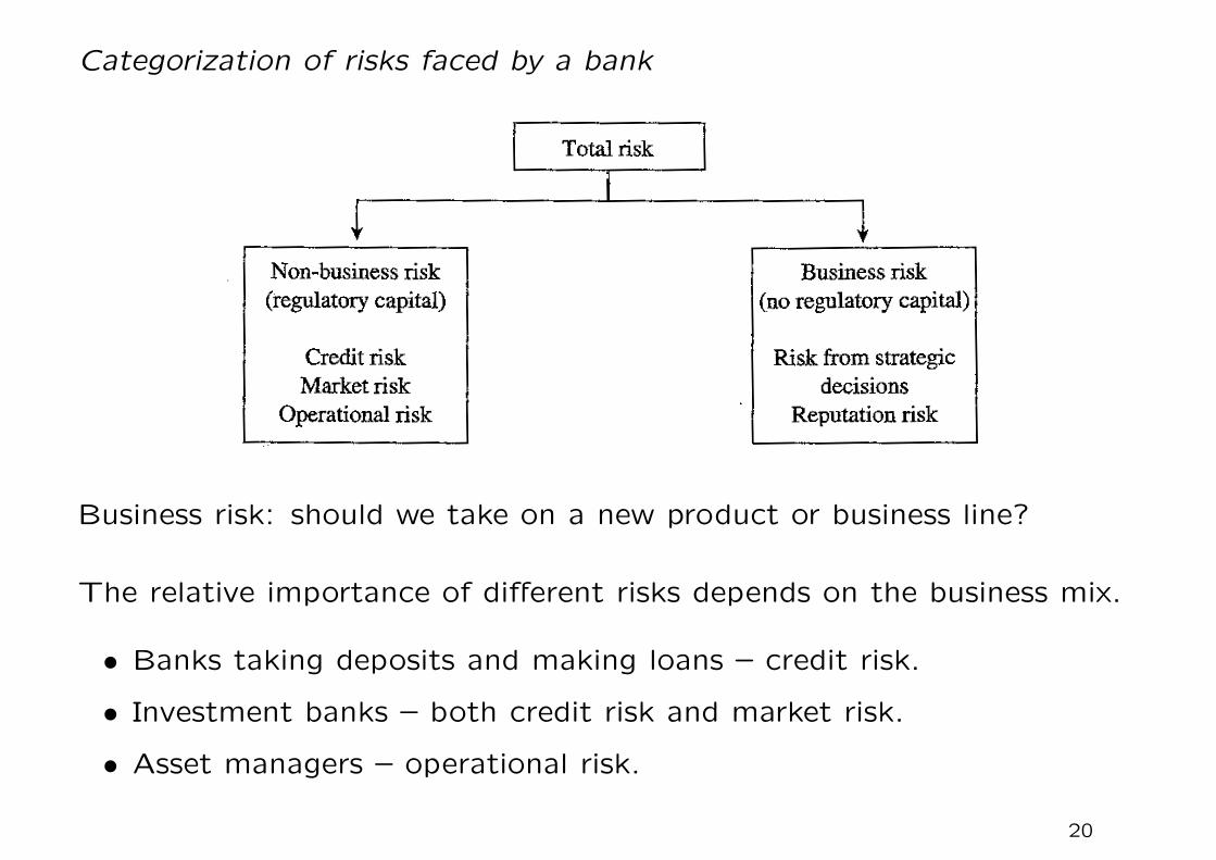
Categorization of risks faced by a bank
Business risk: should we take on a new product or business line?
The relative importance of different risks depends on the business mix.
• Banks taking deposits and making loans – credit risk.
• Investment banks – both credit risk and market risk.
• Asset managers – operational risk.
20

The Barings Bank Disaster – Operational risk
• Nicholas Leeson, an employee of Barings Bank in the Singapore office
in 1995, had a mandate to look for arbitrage opportunities between
the Nikkei 225 futures prices on the Singapore exchange and the
Osaka exchange. Over time Leeson moved from being an arbitrageur
to being a speculator without anyone in the Barings London head
office fully understanding that he had changed the way he was using
derivatives.
• In 1994, Leeson is thought to have made $20 million for Barings,
one-fifth of the total firm’s profit. He drew a $150,000 salary with a
$1 million bonus.
• He began to make losses, which he was able to hide. He then began to
take bigger speculative positions in an attempt to recover the losses,
but only resulted in making the losses worse.
21

• In the end, Leeson’s total loss was close to 1 billion dollars. As a
result, Barings – a bank that had been in existence for 200 years –
was wiped out.
• Lesson to be learnt: Both financial and nonfinancial corporations
must set up controls to ensure that derivatives are being used for
their intended purpose. Risk limits should be set and the activities
of traders should be monitored daily to ensure that the risk limits are
adhered to.
Similar cases
• Societe Generate lost $6.7 billion in January 2008 after trader Jerome
Kerviel took unauthorized positions on European stock index futures.
• UBS lost $2 billion in September 2011 after Kweku Adoboli took
unauthorized positions on currency swap trades.
22

Long Term Capital Management – Liquidity risk
• Long Term Capital Management (LTCM) is a hedge fund formed in
the mid 1990s. The hedge fund’s investment strategy was known as
convergence arbitrage.
• It would find two bonds, X and Y , issued by the same company
promising the same payoffs, with X being less liquid than Y . The
market always places a value on liquidity. As a result the price of
X would be less than the price of Y . LTCM would buy X, short Y
and wait, expecting the prices of the two bonds to converge at some
future time. Normally, with better liquidity on X provided by LTCM,
price of X moves up while price of Y moves down.
23

• When interest rates increased (decreased), the company expected
both bonds to move down (up) in price by about the same amount, so
that the collateral it paid on bond X would be about the same as the
collateral it received on bond Y . It therefore expected that there would
be no significant outflow of funds as a result of its collateralization
agreements.
• In August 1998, Russia defaulted on its debt and this led to what is
termed a“flight to quality” in capital markets. One result was that
investors valued liquid instruments more highly than usual and the
spreads between the prices of the liquid and illiquid instruments in
LTCM’s portfolio increased dramatically (instead of convergence).
24

• The prices of the bonds LTCM had bought went down and the prices
of those it had shorted increased. LTCM was required to post collat-
eral on both.
• The company was highly leveraged and unable to make the payments
required under the collateralization agreements. The result was that
positions had to be closed out and there was a total loss of about $4
billion.
• If the company had been less highly leveraged, it would probably have
been able to survive the flight to quality and could have waited for
the prices of the liquid and illiquid bonds to become closer (eventual
convergence of prices).
25
European Growth Trust (EGT) – Legal risk
• In 1996, Peter Young was a fund manager at Deutsche Morgan Gren-
fell, a subsidiary of Deutsche Bank. He was responsible for managing
a fund called the European Growth Trust (EGT). It had grown to be
a very large fund and Young had responsibilities for managing over
£1 billion of investors’ money.
• Certain rules were applied to EGT, one of these was that no more
than 10% of the fund could be invested in unlisted securities. Peter
Young violated this rule in a way that, it can be argued, benefited
him personally.
• When the facts were uncovered, he was fired and Deutsche Bank had
to compensate investors. The total cost to Deutsche Bank was over
£200 million.
26

Balance sheet scorings based on drivers of firm’s economic well
being
• future earnings and cashflows
• debts, short-term and long-term liabilities, and financial obligations
• capital structure (leverage)
• liquidity of the firm’s assets
• situation (political, social etc) of the firm’s home country or industry
• management quality, company structure, etc.
Rating on a company relies on the statistical analysis of financial variables
plus soft factors.
27

S&P rating categories
AAA best credit qualityextremely reliable with regard to financial obligations
AA very good credit qualityvery reliable
A more susceptible to economic conditionsstill good credit quality
BBB lowest rating in investment gradeBB caution is necessary
best sub-investment credit qualityB vulnerable to changes in economic conditions
currently showing the ability to meet its financial obligationsCCC currently vulnerable to non-payment
dependent on favorable economic conditionsCC highly vulnerable to a payment defaultC close to or already bankrupt
payments on the obligation currently continuedD payment default on some financial obligation has actually
occurred
• The assignment of a probability default to every rating grade in the
given rating scale is called a rating calibration. However, calibration is
not an easy task for rating methods that are based on financial state-
ments (traditional methods adopted by the top three rating agencies).
At best, these rating agencies provide data of historical corporate bond
defaults.28

Threshold model for default of a credit obligor
29

• In the classical Merton structural model, the ability to pay or dis-
tance to default of an obligor is described as a function of assets and
liabilities.
• If liabilities exceed the financial power of an obligor, either a firm or
an individual, bankruptcy and payment failure will follow.
• Given the dynamics of the ability to pay process and default barrier, we
can estimate the probability that the ability to pay process falls below
the barrier. In this sense, the default probability can be quantified.
30

Characterization of the credit risk of loans
• Financial variables to be considered include
– default probability (DP )
– loss fraction called the loss given default (LGD)
– exposure at default (EAD)
Goal: Derive the portfolio risk based on the information of individual
risks and their correlations.
31

Loss variable
L = EAD × SEV × L
where L = 1D, E[1D] = DP . Here, D is the default event that the
obligor defaults within a certain period of time. We treat severity (SEV )
of loss in case of default as a random variable with E[SEV ] = LGD.
Based on the assumption that the exposure, severity and default event
are independent, the expected loss (EL):
EL = E[L] = E[EAD]× LGD ×DP.
Here, EAD is in general stochastic and E[EAD] is the expectation of
several relevant underlying random variables.
Independence assumption in SEV and 1D may be questionable since DP
becomes high and LGD becomes low during a recession period.
32
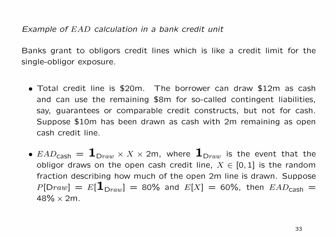
Example of EAD calculation in a bank credit unit
Banks grant to obligors credit lines which is like a credit limit for the
single-obligor exposure.
• Total credit line is $20m. The borrower can draw $12m as cash
and can use the remaining $8m for so-called contingent liabilities,
say, guarantees or comparable credit constructs, but not for cash.
Suppose $10m has been drawn as cash with 2m remaining as open
cash credit line.
• EADcash = 1Draw × X × 2m, where 1Draw is the event that the
obligor draws on the open cash credit line, X ∈ [0,1] is the random
fraction describing how much of the open 2m line is drawn. Suppose
P [Draw] = E[1Draw] = 80% and E[X] = 60%, then EADcash =
48%× 2m.
33

• For the contingent liability part of the credit line, we assume the
existence of a rich database which allows for the calibration of a draw
down factor (DDF), say, 40% for the contingent liability part. Also,
another so-called cash equivalent exposure factor (CEEF) of 80%
which is another conversion factor quantifying the conversion of the
specific contingent liability, say, a guarantee into a cash exposure.
• Finally, we have
E[EAD] = 10m+ 48%× 2m+ 32%× 8m = 13.52m.
.
34
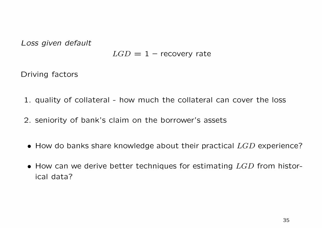
Loss given default
LGD = 1 – recovery rate
Driving factors
1. quality of collateral - how much the collateral can cover the loss
2. seniority of bank’s claim on the borrower’s assets
• How do banks share knowledge about their practical LGD experience?
• How can we derive better techniques for estimating LGD from histor-
ical data?
35

• Assume that a client has m credit products with the bank and pledged
n collateral securities to the bank, called an m-to-n situation.
Remark
It would be difficult to get the interdependence and relation between
products and collateral right (quite often, collateral may be dedicated
to a particular credit product).
• $LGD = (EAD1 + · · ·+ EADm)− ($REC1 + · · ·+$RECn),
where RECi is the recovery proceed from the ith collateral. We have
percentage LGD =$LGD
EAD1 + · · ·+ EADm.
• Technical issues: require a rich database storing historical proceeds
from collateral security categories; also, time value of money should
be considered since recovery proceeds come later.
36

Unexpected loss – standard deviation of L
Holding capital as a cushion against expected losses is not enough. As
a measure of the magnitude of the deviation of losses from the EL, a
natural choice is the standard deviation of the loss variable L, which is
termed unexpected loss.
Unexpected loss (UL) =√var(L) =
√var(EAD × SEV × L).
Under the assumption that the severity and the default event D are inde-
pendent, and also EDA is taken to be deterministic, we have
UL = EAD ×√var(SEV )×DP + LGD2 ×DP (1−DP ).
In contrast to EL, UL is the “actual” uncertainty faced by the bank
when investing in a portfolio since UL captures the deviation from the
expectation.
37
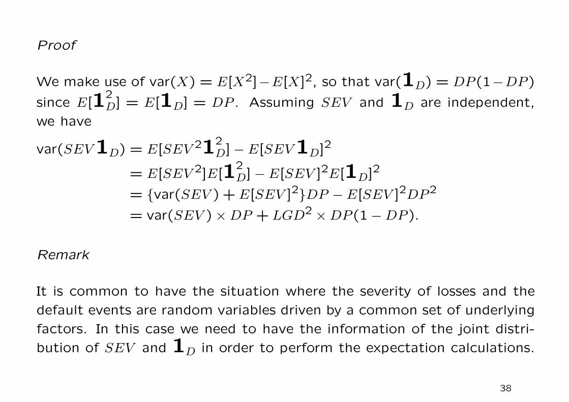
Proof
We make use of var(X) = E[X2]−E[X]2, so that var(1D) = DP (1−DP )
since E[12D] = E[1D] = DP . Assuming SEV and 1D are independent,
we have
var(SEV1D) = E[SEV 212D]− E[SEV1D]2
= E[SEV 2]E[12D]− E[SEV ]2E[1D]2
= {var(SEV ) + E[SEV ]2}DP − E[SEV ]2DP2
= var(SEV )×DP + LGD2 ×DP (1−DP ).
Remark
It is common to have the situation where the severity of losses and the
default events are random variables driven by a common set of underlying
factors. In this case we need to have the information of the joint distri-
bution of SEV and 1D in order to perform the expectation calculations.
38

Portfolio losses
Consider a portfolio of m loans
Li = EADi × SEVi ×1Di, i = 1, . . . ,m, P [Di] = E[1Di] = DPi.
The random portfolio loss Lp is given by
Lp =m∑i=1
Li =m∑i=1
EADi × SEVi × Li, Li =1Di.
Using the additivity of expectation, we obtain
ELp =m∑i=1
ELi =m∑i=1
EADi × LGDi ×DPi.
In the case UL, additivity holds if the loss variable Li are pairwise uncor-
related. Unfortunately, correlations are the “main part of the game” and
a main driver of credit risk.
39

In general, we have
ULp =√var(Lp)
=
√√√√√ m∑i=1
m∑j=1
EADi × EADj × cov(SEVi × Li, SEVj × Lj).
For a portfolio with constant severities, we have the following simplified
formula
UL2p =
m∑i=1
m∑j=1
EADi×EADj×LGDi×LGDj×√DPi(1−DPi)DPj(1−DPj)ρij,
where
ρij = correlation coefficient between default events
=cov(1Di,1Dj)√var(Li)var(Lj)
,
with var(Li) = DPi(1−DPi).
40
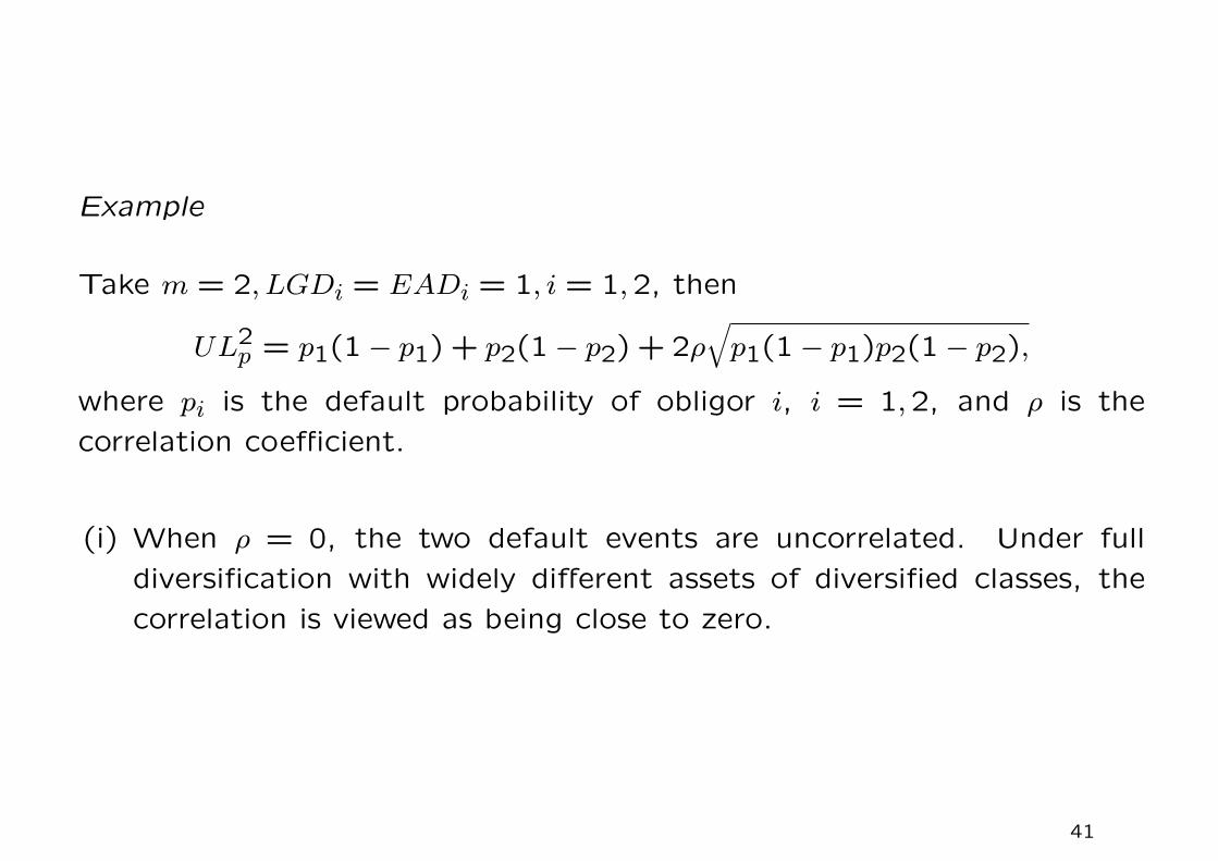
Example
Take m = 2, LGDi = EADi = 1, i = 1,2, then
UL2p = p1(1− p1) + p2(1− p2) + 2ρ
√p1(1− p1)p2(1− p2),
where pi is the default probability of obligor i, i = 1,2, and ρ is the
correlation coefficient.
(i) When ρ = 0, the two default events are uncorrelated. Under full
diversification with widely different assets of diversified classes, the
correlation is viewed as being close to zero.
41
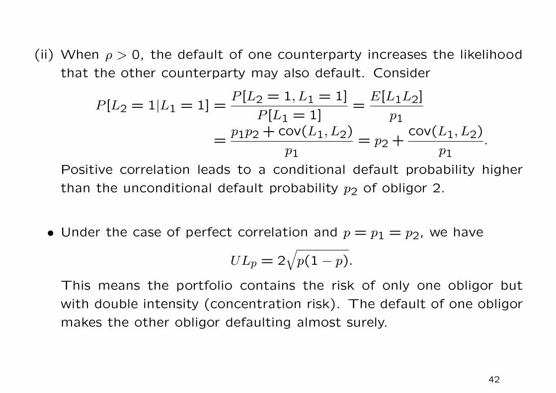
(ii) When ρ > 0, the default of one counterparty increases the likelihood
that the other counterparty may also default. Consider
P [L2 = 1|L1 = 1] =P [L2 = 1, L1 = 1]
P [L1 = 1]=E[L1L2]
p1
=p1p2 + cov(L1, L2)
p1= p2 +
cov(L1, L2)
p1.
Positive correlation leads to a conditional default probability higher
than the unconditional default probability p2 of obligor 2.
• Under the case of perfect correlation and p = p1 = p2, we have
ULp = 2√p(1− p).
This means the portfolio contains the risk of only one obligor but
with double intensity (concentration risk). The default of one obligor
makes the other obligor defaulting almost surely.
42
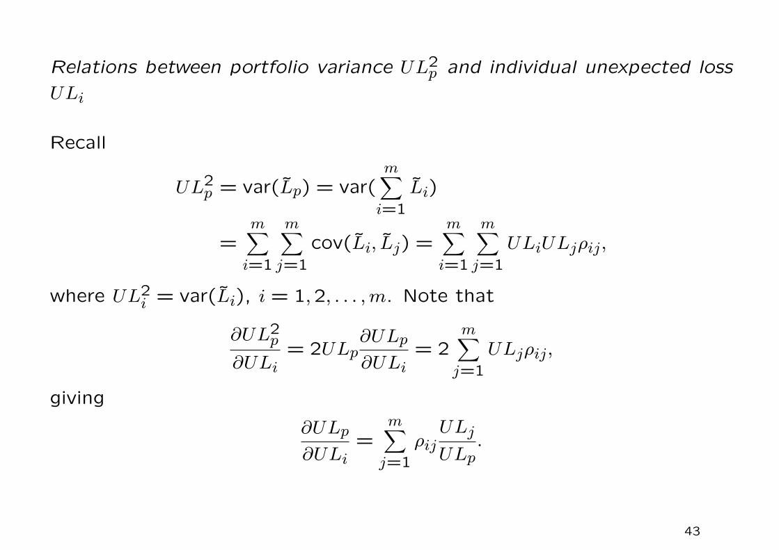
Relations between portfolio variance UL2p and individual unexpected loss
ULi
Recall
UL2p = var(Lp) = var(
m∑i=1
Li)
=m∑i=1
m∑j=1
cov(Li, Lj) =m∑i=1
m∑j=1
ULiULjρij,
where UL2i = var(Li), i = 1,2, . . . ,m. Note that
∂UL2p
∂ULi= 2ULp
∂ULp
∂ULi= 2
m∑j=1
ULjρij,
giving
∂ULp
∂ULi=
m∑j=1
ρijULj
ULp.
43
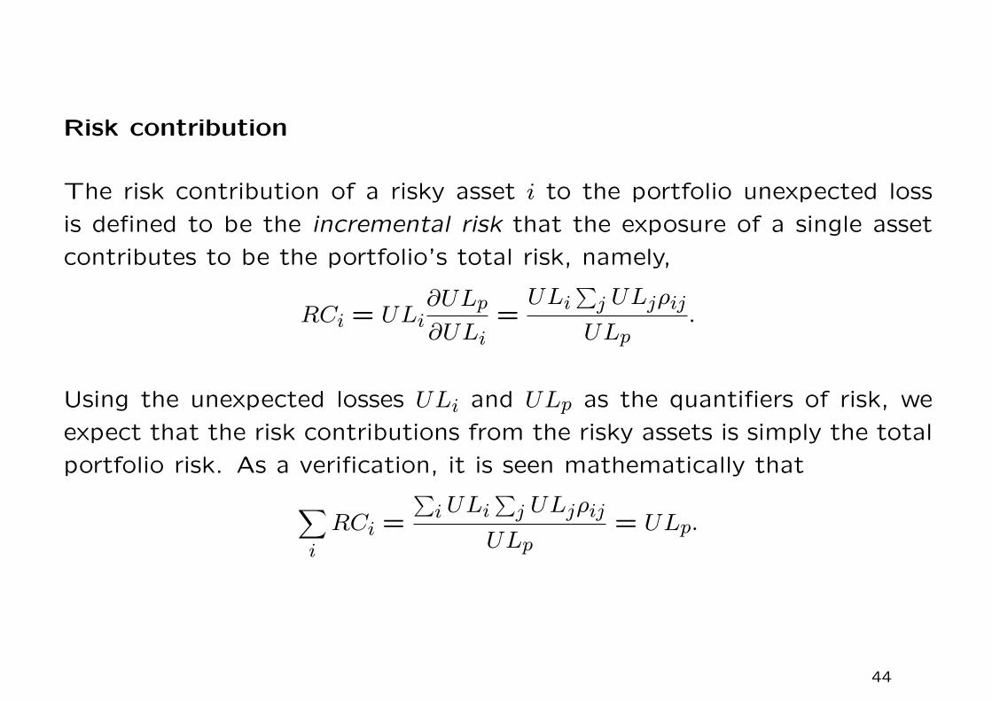
Risk contribution
The risk contribution of a risky asset i to the portfolio unexpected loss
is defined to be the incremental risk that the exposure of a single asset
contributes to be the portfolio’s total risk, namely,
RCi = ULi∂ULp
∂ULi=ULi
∑j ULjρij
ULp.
Using the unexpected losses ULi and ULp as the quantifiers of risk, we
expect that the risk contributions from the risky assets is simply the total
portfolio risk. As a verification, it is seen mathematically that∑i
RCi =
∑iULi
∑j ULjρij
ULp= ULp.
44

Calculation of EL, UL and RC for a two-asset portfolio
ρ default correlation coefficient between the two exposures
ELpportfolio expected loss
ELp = EL1 + EL2
ULpportfolio unexpected loss
ULp =√UL2
1 + UL22 +2ρUL1UL2
RC1risk contribution from Exposure 1
RC1 = UL1(UL1 + ρUL2)/ULp
RC2risk contribution from Exposure 2
RC2 = UL2(UL2 + ρUL1)/ULp
ULp = RC1 +RC2
45

Features of portfolio risk
• The variability of default risk within a portfolio is substantial.
• The correlation between default risks is generally low.
• The default risk itself is dynamic and subject to large fluctuations.
• Default risks can be effectively managed through diversification.
• Within a well diversified portfolio, the loss behavior is characterized
by lower than expected default credit losses for much of the time but
very large losses which are incurred infrequently.
46
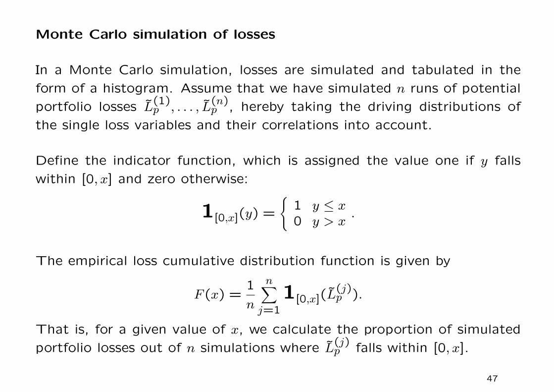
Monte Carlo simulation of losses
In a Monte Carlo simulation, losses are simulated and tabulated in the
form of a histogram. Assume that we have simulated n runs of potential
portfolio losses L(1)p , . . . , L
(n)p , hereby taking the driving distributions of
the single loss variables and their correlations into account.
Define the indicator function, which is assigned the value one if y falls
within [0, x] and zero otherwise:
1[0,x](y) =
{1 y ≤ x0 y > x
.
The empirical loss cumulative distribution function is given by
F (x) =1
n
n∑j=1
1[0,x](L(j)p ).
That is, for a given value of x, we calculate the proportion of simulated
portfolio losses out of n simulations where L(j)p falls within [0, x].
47
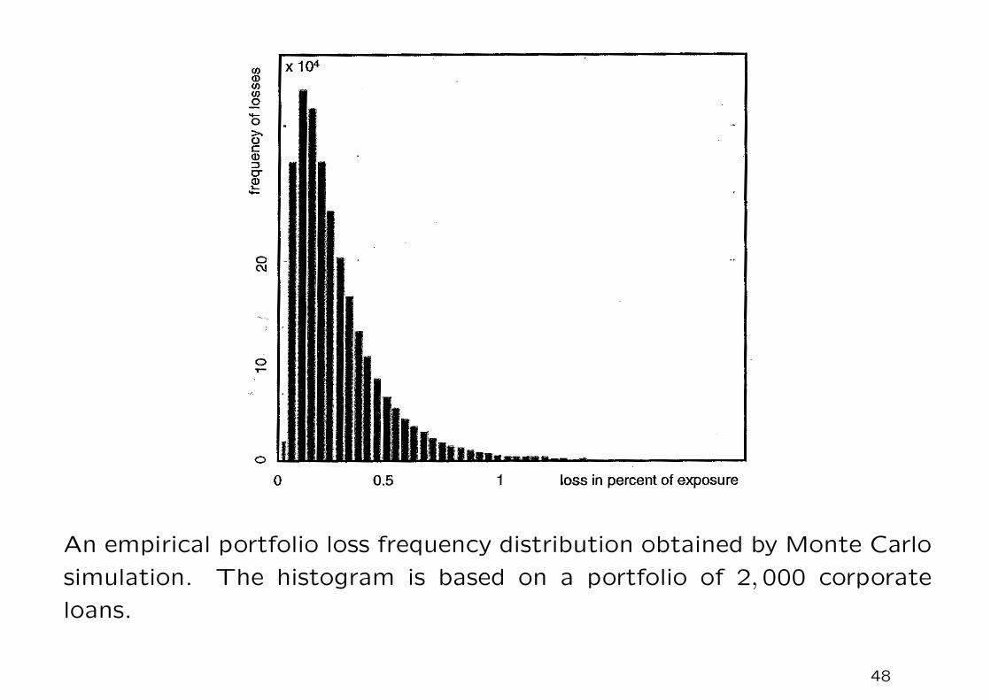
An empirical portfolio loss frequency distribution obtained by Monte Carlo
simulation. The histogram is based on a portfolio of 2,000 corporate
loans.
48

Monte Carlo simulation of loss distribution of a portfolio
1. Estimate default probability and losses
Assign risk ratings to loss facilities and determine their default prob-
ability. Also, assign specified values of LGDs and σsLGD.
2. Estimate asset correlation between obligors
Determine pairwise asset correlation whenever possible or assign oblig-
ors to industry groupings, then determine industry pair correlation.
For example, every obligor in Industry A and every obligor in Industry
B share the same correlation ρAB.
49
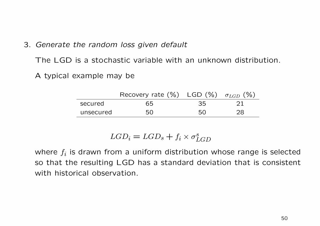
3. Generate the random loss given default
The LGD is a stochastic variable with an unknown distribution.
A typical example may be
Recovery rate (%) LGD (%) σLGD (%)
secured 65 35 21
unsecured 50 50 28
LGDi = LGDs+ fi × σsLGD
where fi is drawn from a uniform distribution whose range is selected
so that the resulting LGD has a standard deviation that is consistent
with historical observation.
50

Generation of correlated default events
1. Generate a set of random numbers drawn from a standard normal
distribution.
2. Perform a cholesky decomposition on the asset correlation matrix
to transform the independent set of random numbers (stored in the
vector e) into a set of correlated asset values (stored in the vector
e′). Recall that the covariance matrix Σ is symmetric and positive
definite (neglect the unlikely event that Σ has the zero eigenvalue).
By performing the usual LDU factorization, we have
Σ = LDU = L√D√DLT =MMT ,
where√D is the diagonal matrix whose diagonal entries are the pos-
itive square roots of those in D, and M = L√D. We compute e′ via
the transformation: e′ =Me. As a check, we consider the covariance
matrix of e′:
E[e′e′T ] = E[MeeTMT ] =ME[eeT ]MT =MIM = Σ.
51
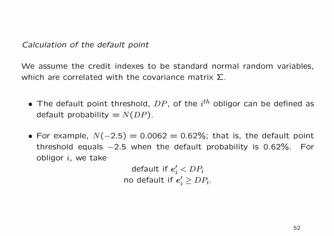
Calculation of the default point
We assume the credit indexes to be standard normal random variables,
which are correlated with the covariance matrix Σ.
• The default point threshold, DP , of the ith obligor can be defined as
default probability = N(DP ).
• For example, N(−2.5) = 0.0062 = 0.62%; that is, the default point
threshold equals −2.5 when the default probability is 0.62%. For
obligor i, we take
default if e′i < DPino default if e′i ≥ DPi.
52
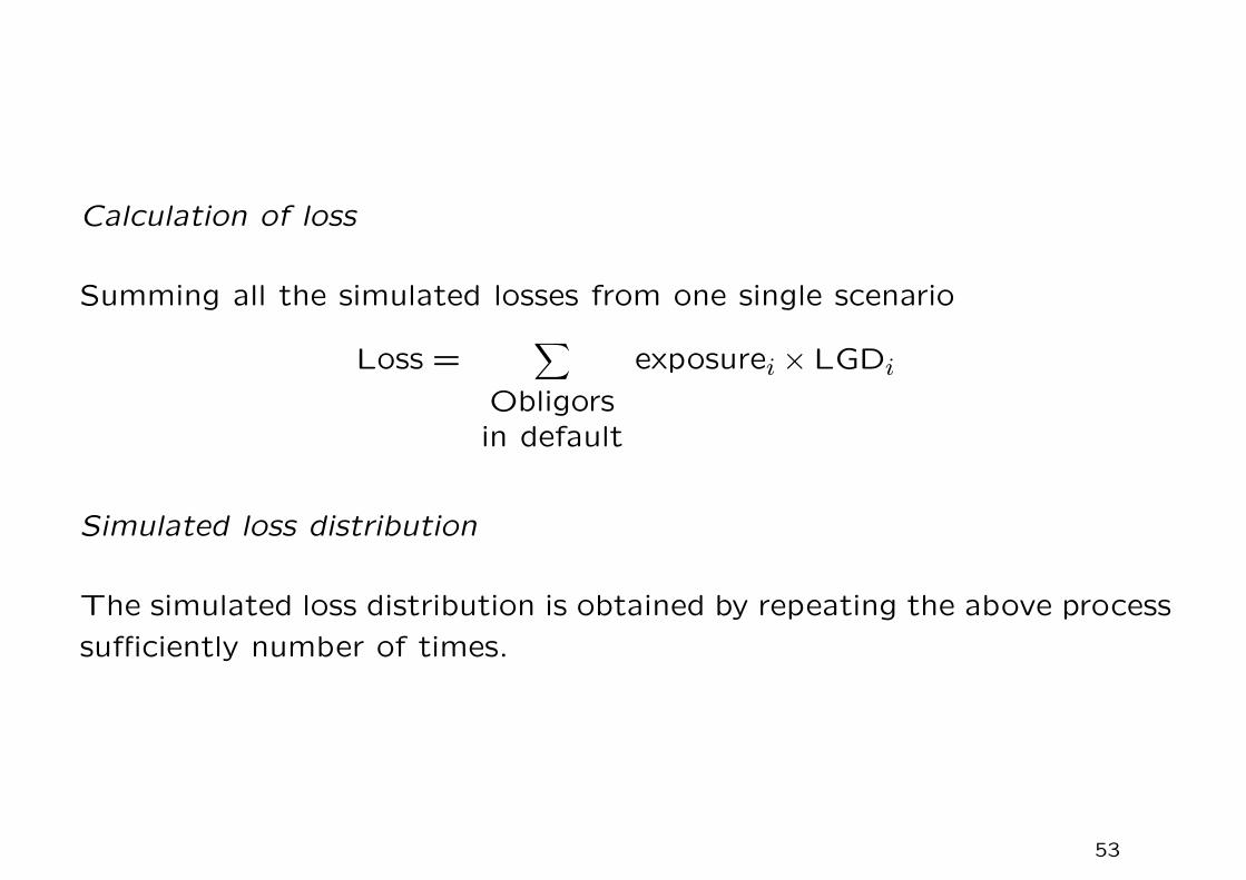
Calculation of loss
Summing all the simulated losses from one single scenario
Loss =∑
Obligorsin default
exposurei × LGDi
Simulated loss distribution
The simulated loss distribution is obtained by repeating the above process
sufficiently number of times.
53

Fitting of loss distribution
The two statistical measures about the credit portfolio are
1. mean, or called the portfolio expected loss;
2. standard deviation, or called the portfolio unexpected loss.
At the simplest level, we approximate the loss distribution of the original
portfolio by a beta distribution through matching the first and second
moments of the portfolio loss distribution.
The risk quantiles of the original portfolio can be approximated by the
respective quantities of the approximating random variable X. The price
for such convenience of fitting is model risk.
Reservation
A beta distribution with only two degrees of freedom is perhaps insufficient
to give an adequate description of the tail events in the loss distribution.
54

Beta distribution
The density function of a beta distribution is
f(x, α, β) =
Γ(α+β)Γ(α)Γ(β)x
α−1(1− x)β−1, 0 < x < 1
0 otherwiseα > 0, β > 0,
where Γ(α) =∫∞0 e−xxα−1 dx.
Mean µ = αα+β and variance σ2 = αβ
(α+β)2(α+β+1).
55

Third and fourth order moments of a distribution
• Skewness describes the departure from symmetry:
γ =
∫∞−∞(x− E[X])3f(x) dx
σ3.
The skewness of a normal distribution is zero. Positive skewness
indicates that the distribution has a long right tail and so entails large
positive values.
• Kurtosis describes the degree of flatness of a distribution:
δ =
∫∞−∞(x− E[X])4f(x) dx
σ4.
The kurtosis of a normal distribution is 3. A distribution with kurtosis
greater than 3 has the tails decay less quickly than that of the normal
distribution, implying a greater likelihood of large value in both tails.
56

Characteristics of loss distributions for different risk types
Type of risk Second moment Third moment Fourth moment
(standard deviation) (skewness) (kurtosis)
Market risk High Zero Low
Credit risk Moderate Moderate Moderate
Operational risk Low High High
• The market risk loss distribution is symmetrical but not perfectly
normally distributed.
57
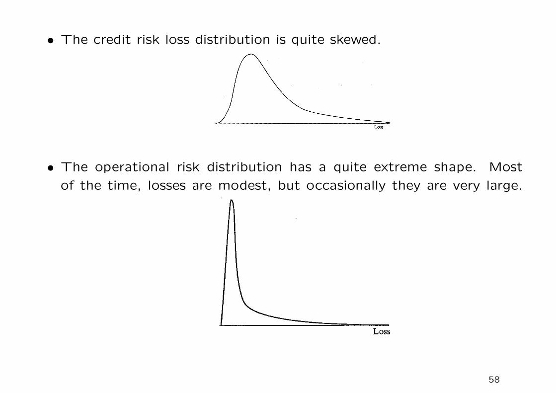
• The credit risk loss distribution is quite skewed.
• The operational risk distribution has a quite extreme shape. Most
of the time, losses are modest, but occasionally they are very large.
58

Loss distribution of a credit portfolio
• All risk quantities on a portfolio level are based on the portfolio loss
variable Lp. Once the loss distribution is generated, all risk measures
can be calculated (details to be discussed in Topic 2.3).
59
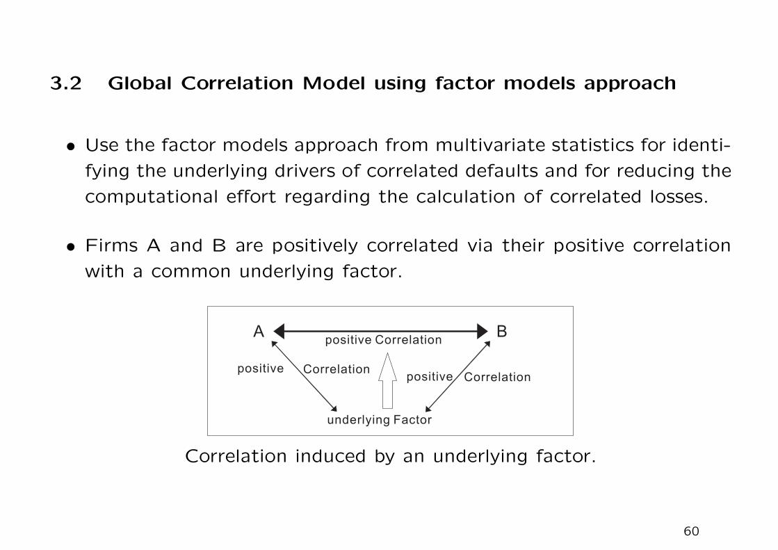
3.2 Global Correlation Model using factor models approach
• Use the factor models approach from multivariate statistics for identi-
fying the underlying drivers of correlated defaults and for reducing the
computational effort regarding the calculation of correlated losses.
• Firms A and B are positively correlated via their positive correlation
with a common underlying factor.
A B
underlying Factor
positive Correlation
positive Correlation
positive Correlation
Correlation induced by an underlying factor.
60
Example – Automotive Industry
• DaimlerChryler is influenced by a factor for Germany, US and some
factors incorporating Aerospace and Financial Companies.
• BMW is correlated with a country factor for Germany and some other
factors.
The underlying factors should be interpretable. For example, suppose
the automotive industry faces pressure, DaimlerChryler and BMW are
also under pressure at the same time.
• The part of the volatility of a company’s asset value process related to
systematic factors like industries or countries is called the systematic
risk of the firm.
• The other part of the firm asset’s volatility that cannot be explained
by systematic influences is called the specific or idiosyncratic risk of
the firm.
61

Three-level factor structure in the Global Correlation Model.
62

1. First level decomposition
• Decomposition of a firm’s variance in a systematic and a specific
part.
Consider the asset value log-return ri of obligor i, as represented by
ri = βiϕi+ ϵi, i = 1,2, . . . ,m. (1)
Here, ϕi is called the composite factor of firm i and βi is the factor
sensitivity. In multi-factor models, ϕi typically is a weighted sum of several
factors. Also, we assume ϕi to be uncorrelated with ϵi, the residual part
of ri.
The equation can be interpreted as a standard linear regression equation,
where βi captures the linear correlation of ri and ϕi. This can be easily
verified as follows:
cov(ri, ϕi) = βivar(ϕi) + cov(ϵi, ϕi)
so that βi = cov(ri, ϕi)/var(ϕi).
In CAPM, βi is called the beta of obligor i.
63

Taking variances on both sides of (1), we have
var(ri) = β2i var(ϕi) + var(ϵi), i = 1,2, . . . ,m.
The first term captures the variability of ri coming from the variability
of the composite factor (systematic risk). The second term arises from
the variability of the residual variable, var(ϵi), which is usually called the
specific risk.
Define
R2i =
β2i var(ϕi)
var(ri)
so that the residual part of the total variance of ri is 1−R2i .
We may write
r = BΦ+ ϵ,
where Φ = (ϕ1 · · ·ϕm)T and B is a diagonal matrix in Rm×m whose diagonal
elements are Bii = βi, i = 1,2, . . . ,m.
64
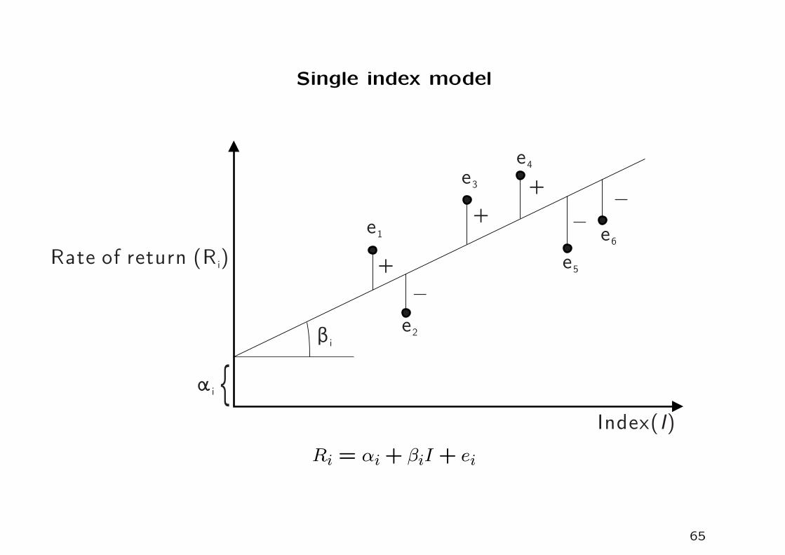
Single index model
β i
α i {
+
+
+
_
__
e1
e2
e3
e4
e5
e6
Index( )I
Rate of return (R )i
Ri = αi+ βiI + ei
65
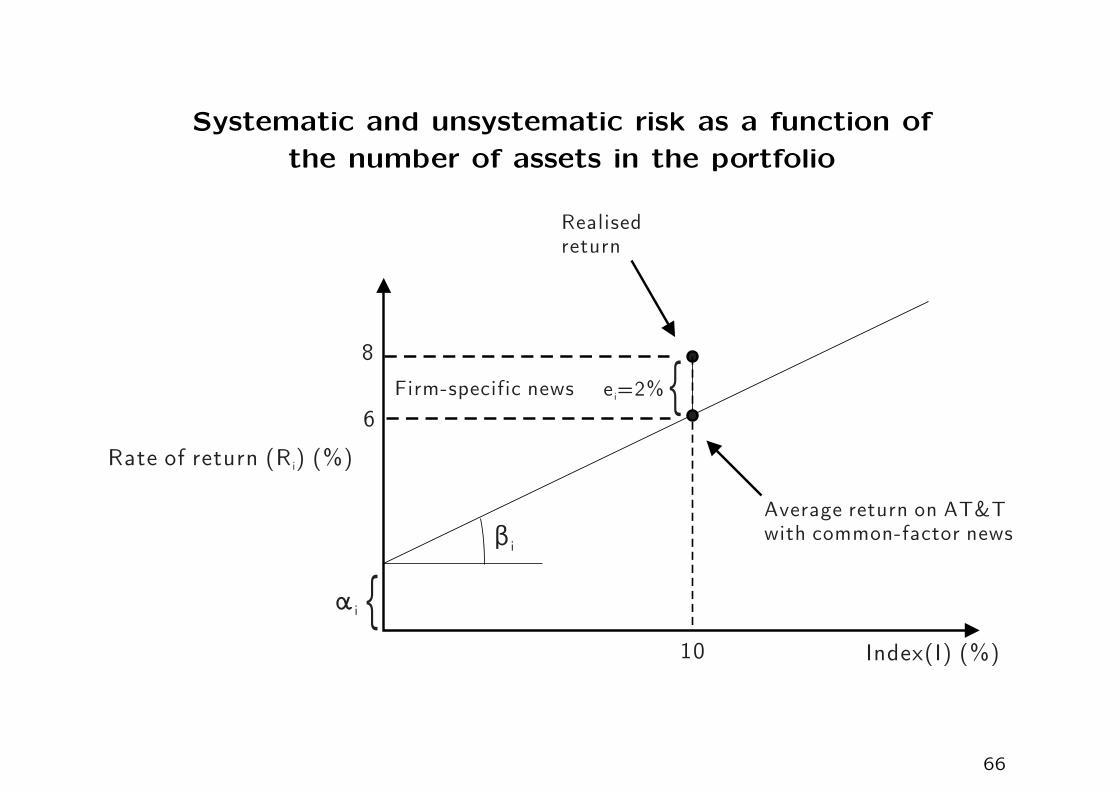
Systematic and unsystematic risk as a function of
the number of assets in the portfolio
β i
α i {Index(I) (%)
Rate of return (R ) (%)i
6
8
{Firm-specific news e =2%i
10
Average return on AT&Twith common-factor news
Realisedreturn
66

2. Second-level decomposition
We decompose each composite factor ϕi with respect to industry and
country breakdown, where
ϕi =K∑k=1
wikψk, i = 1,2, . . . ,m.
Here, ψ1, . . . , ψK0are industry indexes and ψK0+1, . . . , ψK are country
indexes. The industry weights and country weights are summed to
one, that is,
K0∑k=1
wik =K∑
k=K0+1
wik = 1, i = 1,2, . . . ,m.
Define W = (wik)i=1,...,m;k=1,...,K so that
r = BWψ+ ϵ,
where ψ = (ψ1 . . . ψK)T is the vector of industry and country indexes.
67

3. Third-level decomposition
We decompose each industry or country index into a weighted sum
of independent global factors plus residuals, where
ψk =N∑n=1
CknΓn+ δk, k = 1,2, . . . ,K.
In vector notation, we have
Ψ = CΓ+ δ,
where C = (Ckn)k=1,...,K;n=1,...,N denotes the matrix of industry and
country betas, Γ = (Γ1 . . .ΓN)T is the global factor vector, and δ =
(δ1 . . . δK)T is the vector of industry and country residuals. Putting all
relations together:
r = BW (CΓ+ δ) + ϵ.
68

Examples of factors
• S & P index
• US inflation rates
• aggregate sales
• oil prices
• US/Euro exchange rate
• return in long position in small capital stocks less return on large
capital stocks
69

Normalization of asset value log-returns
Define
ri =ri − E[ri]
σi, where σ2i = var(ri), i = 1,2, . . . ,m.
We then write
ri =βiσiϕi+
ϵiσi, where E[ϕi] = E[ϵi] = 0.
The asset correlation is given by
cov(ri, rj) = E[rirj] =βiσi
βj
σjE[ϕiϕj],
since the residual ϵi is uncorrelated to the composite factors. Note that
R2i =
β2iσ2i
var(ϕi)
so that
cov(ri, rj) =Ri√
var(ϕi)
Rj√var(ϕj)
E[ϕiϕj].
70

The normalized quantities are related by
r = BW (CΓ+ δ) + ϵ,
where B is obtained by scaling every diagonal element in B by 1/σi, and
E[Γ] = E [ϵ] = E[δ] = 0.
The asset correlation matrix is obtained by computing
E[ΦΦT ] =W (CE[ΓΓT ]CT + E[δδT])WT .
Note that E[ΓΓT ] is a diagonal matrix with diagonal elements var(Γn),
n = 1,2, . . . , N , and E[δδT] is a diagonal matrix with diagonal element
var(δk), k = 1,2, . . . ,K. This is because we are dealing with uncorrelated
global factors and uncorrelated residuals.
71

3.3 VaR (value-at-risk), expected shortfall and coherent risk mea-
sure
In simple terminology, the value-at-risk measure can be translated as
“I am X percent certain there will not be a loss of more than V dollars in
the next N days.” In essence, it asks the simple question:“How bad can
things get?”.
• The variable V is the VaR of the portfolio. It is a function of (i) time
horizon (N days); (ii) confidence level (X%).
• It is the loss level over N days that has a probability of only (100−X)%
of being exceeded.
• Bank regulators require banks to calculate VaR for market risk with
N = 10 and X = 99.
72

• Weakness of volatility as the measure of risk: it does not care about
the direction of portfolio value movement.
Calculation of VaR from the probability distribution of the change in
the portfolio value; confidence level is X%. Gains in portfolio value are
positive; losses are negative.
73
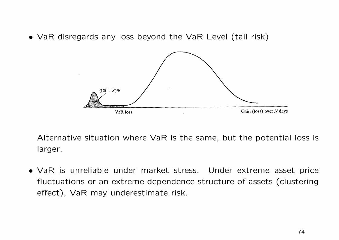
• VaR disregards any loss beyond the VaR Level (tail risk)
Alternative situation where VaR is the same, but the potential loss is
larger.
• VaR is unreliable under market stress. Under extreme asset price
fluctuations or an extreme dependence structure of assets (clustering
effect), VaR may underestimate risk.
74
Formal definition
VaR is defined for a probability measure P and some confidence level α
as the α-quantile of a loss random variable X
varα(X) = inf{x ≥ 0|P [X ≤ x] ≥ α}.
For example, take α = 99% and one-month horizon; the above definition
states that with 99% chance that the loss amount (value of X) is less
than VaRα(X) within the one-month period.
Banks should hold some capital cushion against unexpected losses. Using
UL is not sufficient since there might be a significant likelihood that
losses will exceed portfolio’s EL by more than one standard deviation of
the portfolio loss. Unlike VaR, there is no consideration of confidence
level in this type of risk measure.
• Unfortunately, all risk measures that rely on one absolute value and
a single probability (confidence level) are subject to game playing by
fund managers.
75

Example 1 – Portfolio gain treated as a normal random variable
Suppose that the gain from a portfolio during six months is normally
distributed with a mean of $2 million and a standard deviation of $10
million.
Recall the cumulative normal distribution:
N(x) =∫ x
−∞
1√2π
e−t2/2 dt,
and N(−2.33) = 0.01 = 1%.
• From the properties of the normal distribution, the one-percentile
point of this distribution is 2− 2.33× 10, or -$21.3 million.
• The VaR for the portfolio with a time horizon of six months and
confidence level of 99% is therefore $21.3 million.
76

Example 2
Suppose that for a one-year project all outcomes between a loss $50
million and a gain of $50 million are considered equally likely.
• The loss from the project has a uniform distribution extending from
−$50 million to +$50 million. There is a 1% chance that there will
be a loss greater than $49 million.
• The VaR with a one-year time horizon and a 99% confidence level is
therefore $49 million.
77

Calculation of VaR using historical simulation
Suppose that VaR is to be calculated for a portfolio using a 1-day time
horizon, a 99% confidence level, and 501 days of data.
• The first step is to identify the market variables affecting the portfolio.
These are typically exchange rates, equity prices, interest rates, etc.
• Data is then collected on the movements in these market variables
over the most recent 501 days. This provides 500 alternative scenarios
for what can happen between today and tomorrow.
• Scenario 1 is where the percentage changes in the values of all vari-
ables are the same as they were between Day 0 and Day 1, scenario
2 is where they are the same as they were between Day 1 and Day 2,
and so on.
78

Data for VaR historical simulation calculation.
DayMarket Market
. . .Market
variable 1 variable 2 variable n
0 20.33 0.1132 . . . 65.37
1 20.78 0.1159 . . . 64.91
2 21.44 0.1162 . . . 65.02
3 20.97 0.1184 . . . 64.90... ... ... ... ...
498 25.72 0.1312 . . . 62.22
499 25.75 0.1323 . . . 61.99
500 25.85 0.1343 . . . 62.10
79

Define vi as the value of a market variable on Day i and suppose that
today is Day m. The ith scenario assumes that the value of the market
variable tomorrow will be vmvivi−1
.
For the first variable, the value today, v500, is 25.85. Also v0 = 20.33 and
v1 = 20.78. It follows that the value of the first market variable in the
first scenario is 25.85 × 20.7820.33 = 26.42. For the second scenario, we have
25.85× 21.4420.78 = 26.67.
80

Scenarios generated for tomorrow (Day 501) using data in the last table.
Scenario Market Market. . .
Market Portfolio value Change in value
number variable 1 variable 2 variable n ($ millions) ($ millions)
1 26.42 0.1375 . . . 61.66 23.71 0.21
2 26.67 0.1346 . . . 62.21 23.12 -0.38
3 25.28 0.1368 . . . 61.99 22.94 -0.56... ... ... ... ... ... ...
499 25.88 0.1354 . . . 61.87 23.63 0.13
500 25.95 0.1363 . . . 62.21 22.87 -0.63
Based on today’s portfolio value of 23,50, the change in portfolio in Day
1 and Day 2 are, respectively, 23.71− 23.50 = 0.21 and 23.12− 23.50 =
−0.38.
81

How to estimate the 1-percentile point of the distribution of changes in
the portfolio value?
Since there are a total of 500 scenarios, we can estimate this as the fifth
worst number in the final column of the table. With confidence level of
95%, the maximum loss does not exceed the fifth worst number. The
N-day VaR for a 99% confidence level is calculated as√N times the 1-day
VaR.
Query
Why the choice of√N? This is associated with the property of dispersion
that grows at square root of time.
82

Expected shortfall
The expected shortfall (tail conditional expectation) with respect to a
confidence level α is defined as
ESα(X) = E[X|X > V aRα(X)].
Define by c = V aRα(X), a critical loss threshold corresponding to some
confidence level α, expected shortfall capital provides a cushion against
the mean value of losses exceeding the critical threshold c.
The expected shortfall focusses on the expected loss in the tail, starting
at c, of the portfolio’s loss distribution.
• When the loss distribution is normal, VaR and expected shortfall give
essentially the same information. Both VaR and ES are multiples of
the standard deviation. For example, VaR at the 99% confidence level
is 2.33σ while ES of the same level is 2.67σ.
83

Expected shortfall: E[X|X > V aRα(X)].
• The computation of the expected shortfall requires the information
on the tail distribution (extreme value distribution).
84

Coherent risk measures
Let X and Y be two random variables, like the dollar loss amount of two
portfolios. A risk measure is called a coherent measure if the following
properties hold:
1. monotonicity
For X ≤ Y, γ(X) ≤ γ(Y )
2. translation invariance
For all X ∈ R, γ(X + x) = γ(X) + x.
This would imply γ(X − γ(X)) = 0 for every loss X ∈ L.
3. positive homogeneity
For all λ > 0, γ(λX) = λγ(X)
4. subadditivity
γ(X + Y ) ≤ γ(X) + γ(Y )
85

Financial interpretation of the four properties
1. Monotonicity: If a portfolio produces a worse result than another port-
folio for every state of the world, its risk measure should be greater.
2. Translation invariance: If an amount of cash K is added to a portfolio,
its risk measure should go down by K. This is seem by setting x = −k,so that γ(X − k) = γ(X)− k.
3. Positive homogeneity: Changing the size of a portfolio by a positive
factor λ, while keeping the relative amounts of different items in the
portfolio the same, should result in the risk measure being multiplied
by λ.
4. Subadditivity: The risk measure for two portfolio after they have
been merged should be no greater than the sum of their risk mea-
sures before they were merged. This property reflects the benefit of
diversification: σ(X + Y ) ≤ σ(X) + σ(Y ), where σ(X) denotes the
standard deviation of X.
86

VaR satisfies the first three conditions. However, it does not always
satisfy the fourth one.
Example 3 – Violation of subaddivity in VaR
Suppose each of two independent projects has a probability of 0.02 of
loss of $10 million and a probability of 0.98 of a loss of $1 million during
a one-year period. Suppose we set the confidence level α to be 97.5%.
In this example, the loss random variable X of single project can assume
two discrete values: $1 million and $10 million.
• Since P [X ≤ 1] = 0.98 and P [X ≤ 10] = 1, so the one-year 97.5%
VaR for each project is $1 million.
87
• When the projects are put in the same portfolio, there is a 0.02 ×0.02 = 0.0004 probability of a loss of $20 million, a 2× 0.02× 0.98 =
0.0392 probability of a loss of $11 million, and a 0.98×0.98 = 0.9604
probability of a loss of $2 million.
• Let Y denote the loss random variable of the two projects. Since
P [Y ≤ 2] = 0.9604, P [Y ≤ 11] = 0.9996 and P [Y ≤ 20] = 1, so the
one-year 97.5% VaR for the portfolio is $11 million.
• The total of the VaRs of the projects considered separately is $2
million. The VaR of the portfolio is therefore greater than the sum of
the VaRs of the projects by $9 million. This violates the subadditivity
condition.
88

Example 4 – Violation of subaddivity in VaR
A bank had two $10 million one-year loans, each of which has a 1.25%
chance of defaulting. If a default occurs, all losses between 0% and 100%
of the principal are equally likely. If the loan does not default, a profit of
$0.2 million is made. To simplify matters, we suppose that if one loan
defaults it is certain that the other loan will not default.
1. Consider first a single loan. This has a 1.25% chance of defaulting.
When a default occurs, the loss experienced is evenly distributed be-
tween zero and $10 million. Conditional on a loss being made, there
is an 80% (0.8) chance that the loss will be greater than $2 million.
Since the probability of a loss is 1.25% (0.0125), the unconditional
probability of a loss greater than $2 million is 0.8× 0.0125 = 0.01 or
1%. The one-year, 99% VaR is therefore $2 million.
89

2. Consider next the portfolio of two loans. Each loan defaults 1.25%
of the time and they never default together so that
P [one loss] = 2× 1.25% = 2.5%
P [two losses] = 0.
Upon occurrence of a loan loss event, the loss amount is uniformly
distributed between zero and $10 million.
• There is a 2.5% (0.025) chance of one of the loans defaulting and
conditional on this event there is an 40% (0.4) chance that the
loss on the loan that defaults is greater than $6 million.
• The unconditional probability of a loss from a default being greater
than $6 million is therefore 0.4× 0.025 = 0.01 or 1%.
90
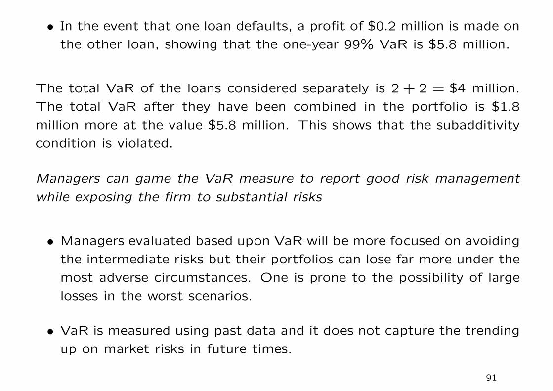
• In the event that one loan defaults, a profit of $0.2 million is made on
the other loan, showing that the one-year 99% VaR is $5.8 million.
The total VaR of the loans considered separately is 2 + 2 = $4 million.
The total VaR after they have been combined in the portfolio is $1.8
million more at the value $5.8 million. This shows that the subadditivity
condition is violated.
Managers can game the VaR measure to report good risk management
while exposing the firm to substantial risks
• Managers evaluated based upon VaR will be more focused on avoiding
the intermediate risks but their portfolios can lose far more under the
most adverse circumstances. One is prone to the possibility of large
losses in the worst scenarios.
• VaR is measured using past data and it does not capture the trending
up on market risks in future times.
91

Example 3 revised – Expected shortfall
In Example 3, the VaR for one of the projects considered on its own is $1
million. To calculate the expected shortfall for a 97.5% confidence level
we note that, of the 2.5% tail of the loss distribution, 2% corresponds to
a loss is $10 million and a 0.5% to a loss of $1 million.
• Conditional that we are in the 2.5% tail of the loss distribution, there
is therefore an 80% probability of a loss of $10 million and a 20%
probability of a loss of $1 million. The expected loss is 0.8×10+0.2×1
or $8.1 million.
• When the two projects are combined, of the 2.5% tail of the loss
distribution, 0.04% corresponds to a loss of $20 million and 2.46%
corresponds to a loss of $11 million. Conditional that we are in
the 2.5% tail of the loss distribution, the expected loss is therefore
(0.04/2.5)×20+(2.46/2.5)×11, or $11.144 million. Since 8.1+8.1 >
11.144, the expected shortfall measure does satisfy the subadditivity
condition for this example.
92

Example 4 revised – Expected shortfall
We showed that the VaR for a single loan is $2 million. The expected
shortfall from a single loan when the time horizon is one year and the
confidence level is 99% is therefore the expected loss on the loan condi-
tional on a loss greater than $2 million is halfway between $2 million and
$10 million, or $6 million.
The VaR for a portfolio consisting of the two loans was calculated in
Example 4 as $5.8 million. The expected shortfall from the portfolio is
therefore the expected loss on the portfolio conditional on the loss being
greater than $5.8 million.
93

• When one loan defaults, the other (by assumption) does not and
outcomes are uniformly distributed between a gain of $0.2 million and
a loss of $9.8 million.
• The expected loss, given that we are in the part of the distribution
between $5.8 million and $9.8 million, is $7.8 million. This is therefore
the expected shortfall of the portfolio.
• Since $7.8 million is less than 2 × $6 million, the expected shortfall
measure does satisfy the subadditivity condition.
The subadditivity condition is not of purely theoretical interest. It is
not uncommon for a bank to find that, when it combines two portfolios
(e.g., its equity portfolio and its fixed income portfolio), the VaR of the
combined portfolio goes up.
94

Impact on risk management with the lack of subadditivity in VaR
• Computing firmwide VaR is often a formidable task to perform. The
alternative is to segment the computations by instruments and risk
drivers, and to compute separate VaR’s on tranches and desks of a
company. This is quite necessary in financial institutions since the
technological trading platforms are often desk by desk.
• With loss of subadditivity, the firmwide VaR cannot be properly as-
sessed.
95
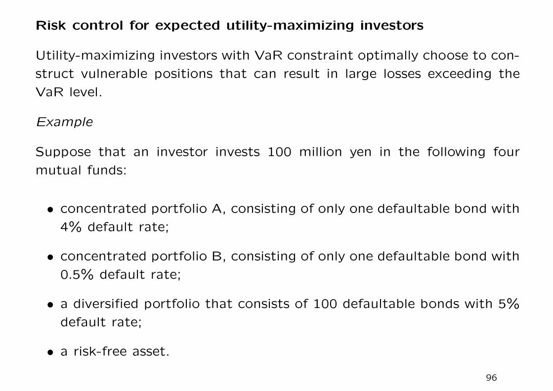
Risk control for expected utility-maximizing investors
Utility-maximizing investors with VaR constraint optimally choose to con-
struct vulnerable positions that can result in large losses exceeding the
VaR level.
Example
Suppose that an investor invests 100 million yen in the following four
mutual funds:
• concentrated portfolio A, consisting of only one defaultable bond with
4% default rate;
• concentrated portfolio B, consisting of only one defaultable bond with
0.5% default rate;
• a diversified portfolio that consists of 100 defaultable bonds with 5%
default rate;
• a risk-free asset.
96
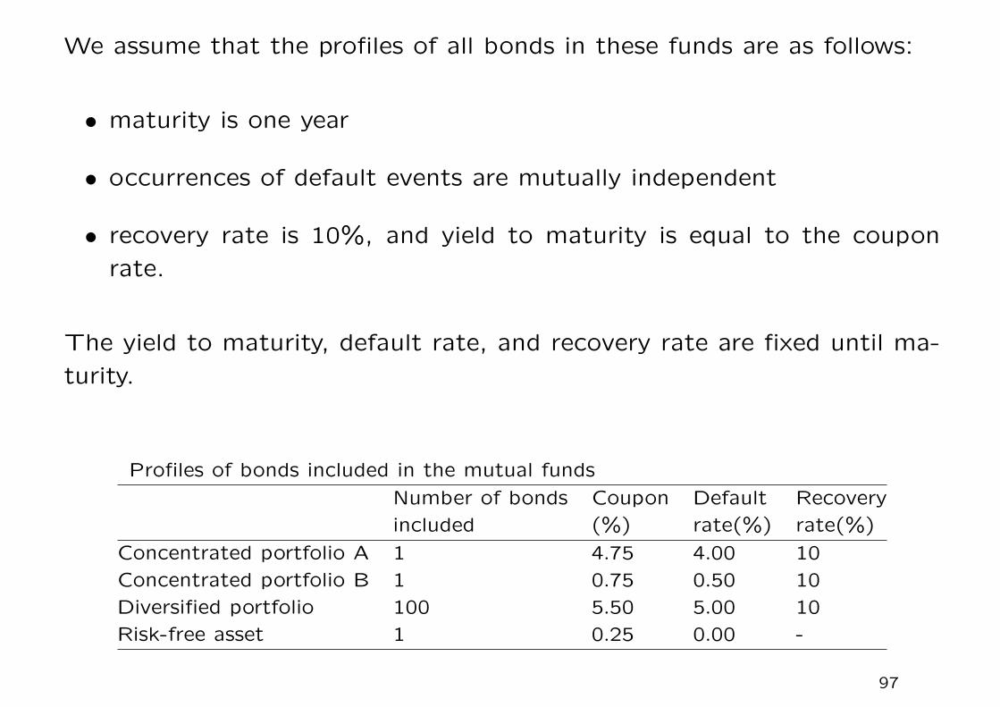
We assume that the profiles of all bonds in these funds are as follows:
• maturity is one year
• occurrences of default events are mutually independent
• recovery rate is 10%, and yield to maturity is equal to the coupon
rate.
The yield to maturity, default rate, and recovery rate are fixed until ma-
turity.
Profiles of bonds included in the mutual funds
Number of bonds Coupon Default Recovery
included (%) rate(%) rate(%)
Concentrated portfolio A 1 4.75 4.00 10
Concentrated portfolio B 1 0.75 0.50 10
Diversified portfolio 100 5.50 5.00 10
Risk-free asset 1 0.25 0.00 -
97

W final wealth,W0 initial wealth,X1 amount invested in concentrated portfolio A,X2 amount invested in concentrated portfolio B,X3 amount invested in diversified portfolio.
Assuming logarithmic utility, the expected utility of the investor is given
below:
E[u(W )] =100∑n=0
0.96 · 0.995 · 0.05n · 0.95100−n ·100 Cn · ln w(1,1)
+100∑n=0
0.04 · 0.995 · 0.05n · 0.95100−n ·100 Cn · ln w(0.1,1)
+100∑n=0
0.96 · 0.005 · 0.05n · 0.95100−n ·100 Cn · ln w(1,0.1)
+100∑n=0
0.04 · 0.005 · 0.05n · 0.95100−n ·100 Cn · ln w(0.1,0.1).
where
w(a, b) =1.0475aX1 +1.0075bX2 +1.055X3100− 0.9n
100+ 1.0025(W0 −X1 −X2 −X3).
98

We analyze the impact of risk management with VaR and expected short-
fall on the rational investor’s decisions by solving the following five opti-
mization problems, where the holding period is one year.
1. No constraint
max{X1X2X3}
E[u(W )].
2. Constraint with VaR at the 95% confidence level
max{X1X2X3}
E[u(W )]
subject to VaR(95% confidence level) ≤ 3.
99

3. Constraint with expected shortfall at the 95% confidence level
max{X1X2X3}
E[u(W )]
subject to expected shortfall(95% confidence level) ≤ 3.5.
4. Constraint with VaR at the 99% confidence level
max{X1X2X3}
E[u(W )]
subject to VaR(99% confidence level) ≤ 3.
5. Constraint with expected shortfall at the 99% confidence level
max{X1X2X3}
E[u(W )]
subject to expected shortfall(99% confidence level) ≤ 3.5.
100
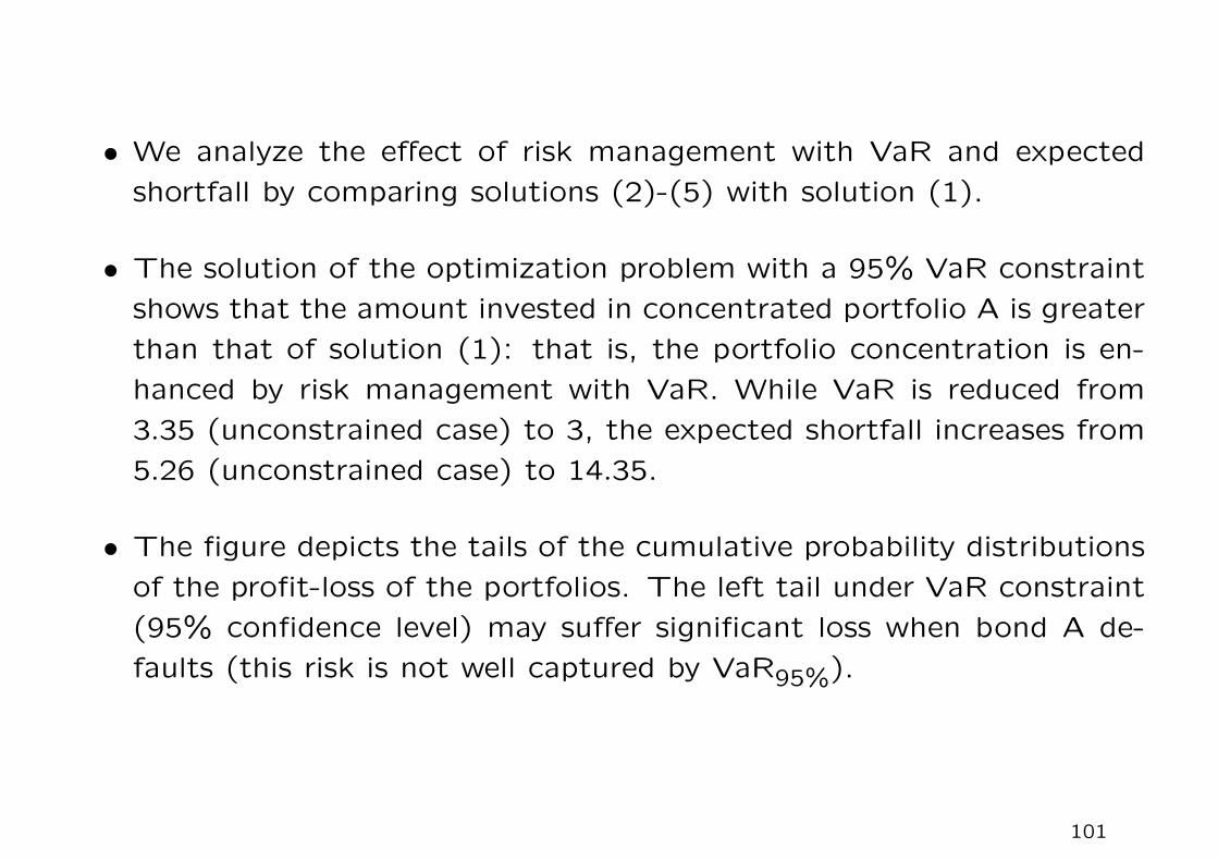
• We analyze the effect of risk management with VaR and expected
shortfall by comparing solutions (2)-(5) with solution (1).
• The solution of the optimization problem with a 95% VaR constraint
shows that the amount invested in concentrated portfolio A is greater
than that of solution (1): that is, the portfolio concentration is en-
hanced by risk management with VaR. While VaR is reduced from
3.35 (unconstrained case) to 3, the expected shortfall increases from
5.26 (unconstrained case) to 14.35.
• The figure depicts the tails of the cumulative probability distributions
of the profit-loss of the portfolios. The left tail under VaR constraint
(95% confidence level) may suffer significant loss when bond A de-
faults (this risk is not well captured by VaR95%).
101

102

Cumulative probability of profit-loss: the left tail (95% confidence level).
The stepwise increments of the cumulative distribution reflect the discrete
loss amount upon default of a name in the portfolio.
103

Under VaR constraint
When constrained by VaR, the investor must reduce her investment in
the diversified portfolio to reduce maximum losses with a 95% confidence
level, and she should increase investments either in concentrated portfolio
or in a risk-free asset.
• Concentrated portfolio A has little effect on VaR, since the probabil-
ity of default lies beyond the 95% confidence interval. Concentrated
portfolio A also yields a higher return than other assets, except diver-
sified portfolio. Thus, the investor chooses to invest in concentrated
portfolio A.
• Although VaR is reduced, the optimal portfolio is vulnerable due to
its concentration and larger losses under conditions beyond the VaR
level.
104

Under expected shortfall constraint
When constrained by expected shortfall, there is a higher chance that
the investor chooses optimally to reallocate his investment to a risk-free
asset, significantly reducing the portfolio risk.
• The investor cannot increase his investment in the concentrated port-
folio without affecting expected shortfall, which takes into account the
losses beyond the VaR level.
• Unlike risk management with VaR, risk management with expected
shortfall does not enhance credit concentration.
105

Raising the confidence level to 99%
• We examine whether raising the confidence level of VaR solves the
problem. The new table gives the results of the optimization problem
with a 99% VaR or expected shortfall constraint. It shows that when
constrained by VaR at the 99% confidence level, the investor optimally
chooses to increase his/her investment in concentrated portfolio B
because the default rate of concentrated portfolio B is 0.5%, outside
the confidence level of VaR.
• Risk management with expected shortfall reduces the potential loss
beyond the VaR level by reducing credit concentration.
• VaR may enhance credit concentration because it disregards losses
beyond the VaR level, even at high confidence levels. On the other
hand, expected shortfall reduces credit concentration because it takes
into account losses beyond the VaR level as a conditional expectation.
106

• With higher confidence level, VaR and ES increase under ”no con-
straint“ case.
107

Cumulative distribution of profit-loss when the tail risk of VaR occurs.
• If investors can invest in assets whose loss is infrequent but large
(such as concentrated credit portfolios), the problem of tail risk can
be serious. Investors can manipulate the profit-loss distribution using
those assets, so that VaR becomes small while the tail becomes fat.108

Spectral risk measure
A risk measure can be characterized by the weights it assigns to quantiles
of the loss distribution.
• VaR gives a 100% weighting to the Xth quantile and zero to other
quantiles.
• Expected shortfall gives equal weight to all quantiles greater than the
Xth quantile and zero weight to all quantiles below Xth quantile.
We can define what is known as a spectral risk measure by making other
assumptions about the weights assigned to quantiles. A general result is
that a spectral risk measure is coherent (i.e., it satisfies the subadditivity
condition) if the weight assigned to the qth quantile of the loss distri-
bution is a nondecreasing function of q. Expected shortfall satisfies this
condition.
109

Proof of subadditivity for the expected shortfall
Let F (x) be a probability distribution of a random variable X, where
F (x) = P [X ≤ x].
For some probability q ∈ (0,1), we define the q-quantile as
xq = inf{x|F (x) ≥ q}.
If F (·) is continuous, we have F (xq) = q, while if F (·) is discontinuous
in xq, with P [X = xq] > 0, we may have F (xq) = P [X ≤ xq] > q. The
definition of q-Tail Mean xq as the ”expected value of the distribution in
the q-quantile“ must take this fact into account.
In the current context, we take X to be the profit / gain (random) variable
of the portfolio. Suppose we let q = 0.05, xq refers to the profit level
(negative in value) that
xq = inf{x|P [X ≤ x] ≥ q}.
That is, with confidence level of 1 − q = 95%, the loss amount is not
more than −xq.110

x
F(x)
x q
q
100%
For a random variable X and for a specified level of probability q, we
define the q-Tail Mean:
xq =1
qE[X1X≤xq] +
[1−
F (xq)
q
]xq =
1
qE[X1q
X≤xq],
where
1qX≤xq =1X≤xq +
q − F (xq)
P [X = xq]1qX=xq.
111

The second term in the sum is zero if P [X = xq] = 0. By virtue of the
above definition, we have
E[1qX≤xq] = q
0 ≤1qX≤zq ≤ 1.
Note that in the case X = xq:
1qX≤xq|X=xq = 1+
q − F (xq)
P [X = xq]=
q − F (x−q )
P [X = xq]∈ [0,1]
since F (x−q ) ≤ q ≤ F (x+q ) = F (xq) and P [X = xq] = F (xq) − F (x−q ) by
definition of xq.
Given two random variables X and Y and defining Z = X + Y , we would
like to establish:
zq ≥ xq + yq.
112

Consider
q(zq − xq − yq) = E[Z1qZ≤zq −X1q
X≤xq − Y1qY≤yq]
= E[X(1qZ≤zq −1q
X≤xq) + Y (1qZ≤zq −1q
Y≤yq)]
≥ xqE[(1qZ≤zq −1q
X≤xq)] + yqE[(1qZ≤zq −1q
Y≤yq)]
= xq(q − q) + yq(q − q) = 0.
In the inequality, we have used 1qZ≤zq −1q
X≤xq ≥ 0, if X > xq
1qZ≤zq −1q
X≤xq ≤ 0, if X < xq.
For any risk measure R defined as
R(X) = f(X)− xq,
where f is a linear function, the subadditive property holds
R(X + Y ) ≤ R(X) +R(Y ).
113

3.4 Economic capital and risk-adjusted return on capital
Definition of economic capital (also called risk capital)
• This is the amount of capital a financial institution needs in order to
absorb losses over a certain time horizon (usually one year) with a
certain confidence level.
• The confidence level depends on financial institutions’ objectives.
Corporations rated AA have a one-year probability of default less than
0.1%. This suggests that the confidence level should be 99.9%, or
even higher.
114

Take a target level of statistical confidence into account. For a given
level of confidence α, let Lp denote the random portfolio loss amount, we
define the credit VaR by the α-quartile of Lp:
qα = inf{q > 0|P [LP ≤ q] ≥ α}.
Also, we define
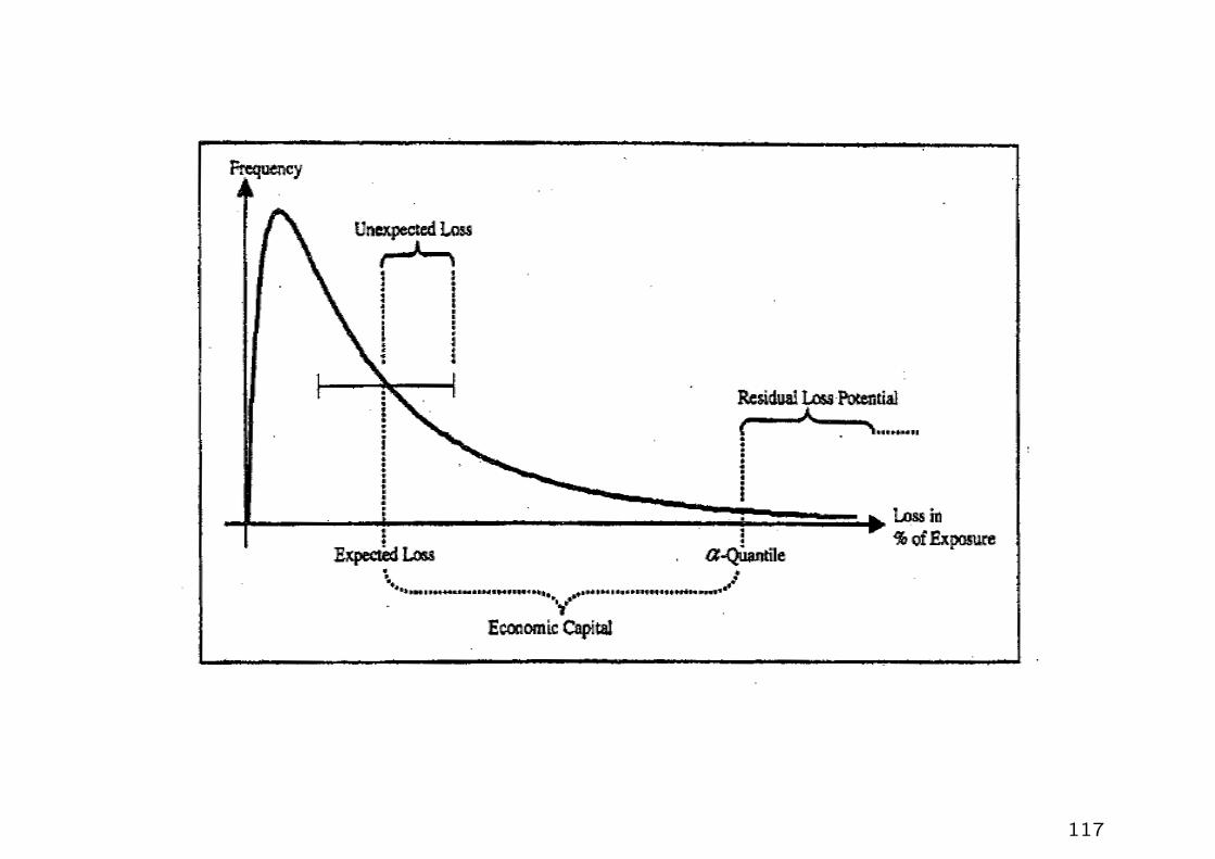
EC = economic capital = qα − ELP .
Say, α = 99.98%, this would mean ECα will be sufficient to cover un-
expected losses in 9,998 out of 10,000 years (!"#$%), assuming a
planning horizon of one year.
115

Why reducing the quantile qα by the EL? This is the usual practice
of decomposing the total risk capital into (i) expected loss (ii) cushion
against unexpected losses.
Note that EL charges are portfolio independent (diversification has no
impact) while EC charges are portfolio dependent. New loans may add a
lot or little risk contributions (risk concentration).
• When lending in a certain region of the world a AA-rated bank esti-
mates its losses as 1% of outstanding loans per year on average. The
99.9% worst-case loss (i.e., the loss exceeded only 0.1% of the time)
is estimated as 5% of outstanding loans. The economic capital re-
quired per $100 of loans made is therefore $4.0. This is the difference
between the 99.9% worst-case loss (VaR99.9% = 5) and the expected
loss.
116
117

Bottom-up approach
The loss distributions are estimated for different types of risk and different
business units and then aggregated.
• The first step in the aggregation is to calculate the probability distri-
butions for losses by risk type or losses by business unit.
• A final aggregation gives a probability distribution of total losses for
the whole financial institution.
Operational risk as ”the risk of loss resulting from inadequate or failed
internal processes, people, and systems or from external events”. Oper-
ational risk includes model risk and legal risk, but it does not include risk
arising from strategic decisions or reputational risk. This type of risk is
collectively referred as business risk. Regulatory capital is not required for
business risk under Basel II, but some banks do assess economic capital
for business risk.
118

Aggregating economic capital
Suppose a financial institution has calculated market, credit, operational,
and (possibly) business risk loss distributions for a number of different
business units.
Question
How to aggregate the loss distributions to calculate a total economic
capital for the whole enterprise?
According to Basel II,
total economic capital, Etotal =n∑i=1
Ei.
This is based on the assumption of perfect correlation between the dif-
ferent types of risks – too conservative.
119

Hybrid approach
Etotal = cov(x1 + · · ·+ xn, x1 + · · ·+ xn)
=
√√√√√ n∑i=1
n∑j=1
EiEjρij,
where we take Ei = σ(xi) as proxy and ρij is the correlation between risk
i and risk j.
• When the distributions are normal, this approach is exact.
Economic capital estimates
Type of risk Business Unit Business Unit
1 2
Market risk 30 40
Credit risk 70 80
Operational risk 30 90
120

Correlations between losses:
MR, CR, and OR refer to market risk, credit risk, and
operational risk; 1 and 2 refer to the business units.
MR-1 CR-1 OR-1 MR-2 CR-2 OR-2
MR-1 1.0 0.5 0.2 0.4 0.0 0.0
CR-1 0.5 1.0 0.2 0.0 0.6 0.0
OR-1 0.2 0.2 1.0 0.0 0.0 0.0
MR-2 0.4 0.0 0.0 1.0 0.5 0.2
CR-2 0.0 0.6 0.0 0.5 1.0 0.2
OR-2 0.0 0.0 0.0 0.2 0.2 1.0
• Correlation between 2 different risk types in 2 different business units
= 0.
• Correlation between market risks across business units = 0.4.
• Correlation between credit risks across business units = 0.6.
• Correlation between operational risks across business units = 0.
121

• Total market risk economic capital is√302 +402 +2× 0.4× 30× 40 = 58.8.
• Total credit risk economic capital is√702 +802 +2× 0.6× 70× 80 = 134.2.
• Total operational risk economic capital is√302 +902 = 94.9.
• Total economic capital for Business Unit 1 is
√302+702+302+2×0.5×30×70+2×0.2×30×30+2×0.2×70×30 = 100.0.
• Total economic capital for Business Unit 2 is
√402+802+902+2×0.5×40×80+2×0.2×40×90+2×0.2×80×90 = 153.7.
122

The total enterprise-wide economic capital is the square root of
302 +402 +702 +802 +302 +902 +2× 0.4× 30× 40+ 2× 0.5× 30× 70
+ 2× 0.2× 30× 30+ 2× 0.5× 40× 80+ 2× 0.2× 40× 90
+ 2× 0.6× 70× 80+ 2× 0.2× 70× 30+ 2× 0.2× 80× 90
which is 203.224.
There are significant diversification benefits. The sum of the economic
capital estimates for market, credit, and operational risk is
58.8+ 134.2+ 94.9 = 287.9,
and the sum of the economic capital estimates for two business units is
100 + 153.7 = 253.7.
Both of these are greater than the total economic capital estimate of
203.2.
123

Risk-adjusted return on capital (RAROC)
Risk-adjusted performance measurement (RAPM) has become an impor-
tant part of how business units are assessed. There are many different
approaches, but all have one thing in common. They compare return
with capital employed in a way that incorporates an adjustment for risk.
The most common approach is to compare expected return with economic
capital. The formula for RAROC is
RAROC =Revenues−Costs− Expected losses
Economic capital.
The numerator may be calculated on a pre-tax or post-tax basis. Some-
times, a risk-free rate of return on the economic capital is calculated and
added to the numerator.
124
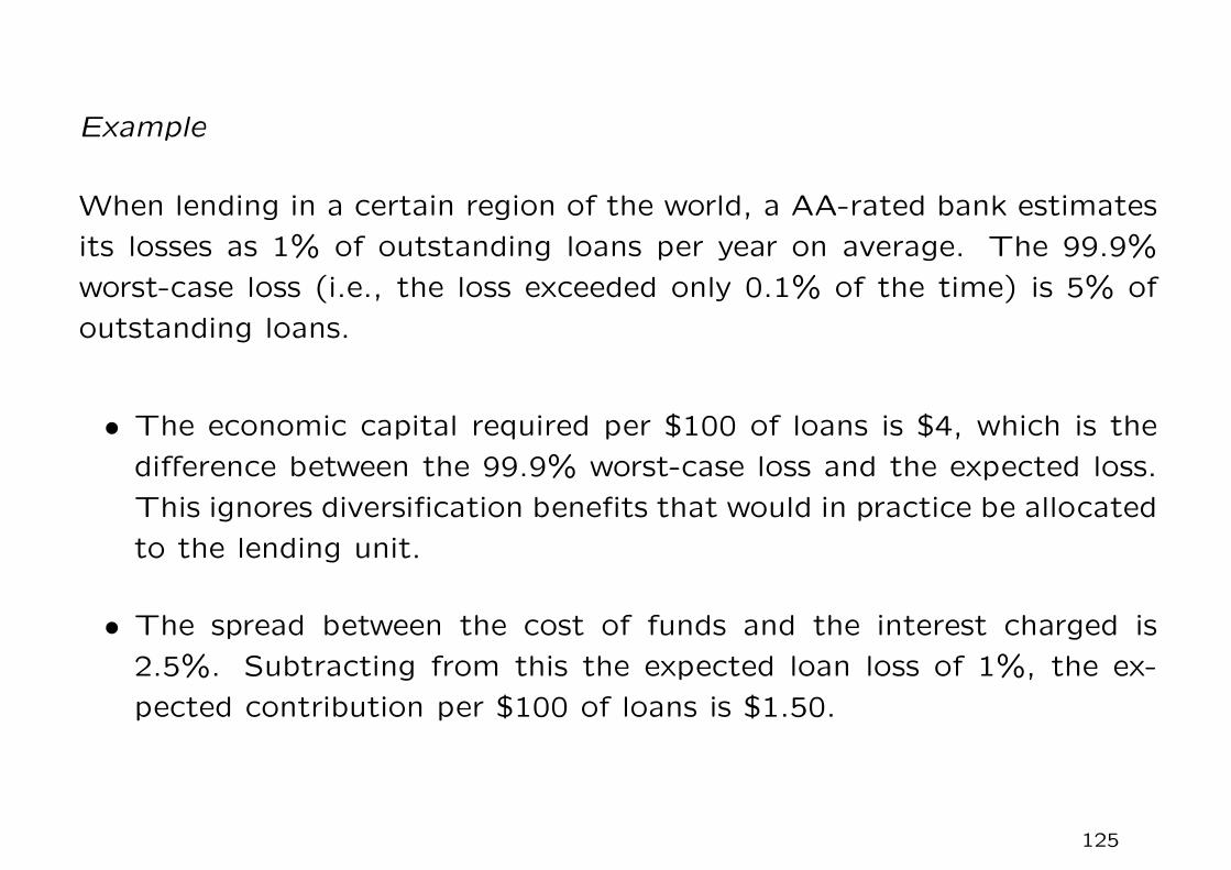
Example
When lending in a certain region of the world, a AA-rated bank estimates
its losses as 1% of outstanding loans per year on average. The 99.9%
worst-case loss (i.e., the loss exceeded only 0.1% of the time) is 5% of
outstanding loans.
• The economic capital required per $100 of loans is $4, which is the
difference between the 99.9% worst-case loss and the expected loss.
This ignores diversification benefits that would in practice be allocated
to the lending unit.
• The spread between the cost of funds and the interest charged is
2.5%. Subtracting from this the expected loan loss of 1%, the ex-
pected contribution per $100 of loans is $1.50.
125

• Assuming that the lending unit’s administrative costs total 0.7% of
the amount loaned, the expected profit is reduced to $0.80 per $100
in the loan portfolio. RAROC is therefore
0.80
4= 20%.
• An alternative calculation would add the interest on the economic
capital to the numerator. Suppose that the risk-free interest rate is
2%. Then 0.02×4 = 0.08 is added to the numerator, so that RAROC
becomes0.88
4= 22%.
126
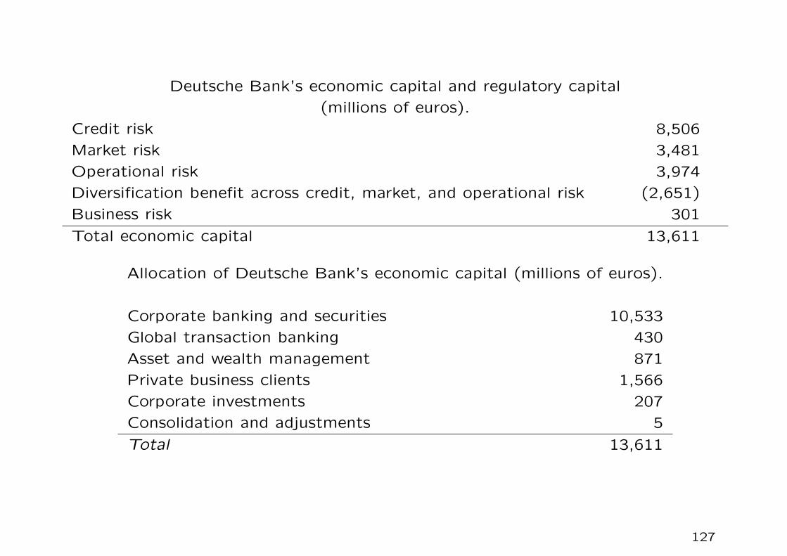
Deutsche Bank’s economic capital and regulatory capital
(millions of euros).
Credit risk 8,506
Market risk 3,481
Operational risk 3,974
Diversification benefit across credit, market, and operational risk (2,651)
Business risk 301
Total economic capital 13,611
Allocation of Deutsche Bank’s economic capital (millions of euros).
Corporate banking and securities 10,533
Global transaction banking 430
Asset and wealth management 871
Private business clients 1,566
Corporate investments 207
Consolidation and adjustments 5
Total 13,611
127

• RAROC can be calculated ex-ante (before the start of the year) or
ex-post (after the end of the year). Ex-ante calculations are based
on estimates of expected profit. Ex-post calculations are based on
actual profit results. Ex-ante calculations are typically used to decide
whether a particular business unit should be expanded or contracted.
Ex-post calculations are typically used for performance evaluation and
bonus calculations.
• It is usually not appropriate to base a decision to expand or contract
a particular business unit on an ex-post analysis (although there is
a natural temptation to do this). It may be that results were bad
for the most recent year because credit losses were much larger than
average or because there was an unexpectedly large operational risk
loss. Key strategic decisions should be based on expected long-term
results.
128

Appendix: Estimation of the annualized realized volatility of stock
prices
The stock price process St is governed by
dSt
St= µ dt+ σ dZt or d lnSt = (µ−
σ2
2)dt+ σ dZt,
where µ is the expected growth rate, σ is the volatility, and Zt is the
standard Brownian process; dZt can be loosely interpreted as ϕ√δt, where
ϕ is the standard normal random variable and δt is the infinitesimal time
increment.
Discrete approximations Write Si = S(ti) and Si−1 = S(ti−1)
dSt
St
∣∣∣∣∣t=ti
≈Si − Si−1
Si,
d lnSt|t=ti ≈ lnSi − lnSi−1 = lnSiSi−1
.
129

Write δt = ti − ti−1 so that
lnSiSi−1
≈ (µ−σ2
2)δt+ σϕ
√δt.
Estimate the volatility of log-return by sampling the logarithm of stock
return over the tenor: [t0, t1, . . . , tN ].
Recall var(X) = E[X2]−E[X]2. The market convention of measuring the
annualized variance of log-return is given by
A
N
N∑i=1
(lnSiSi−1
)2.
Here, the square of the sampled mean is assumed to be negligibly small.
130

The factor A is called the annualization factor that converts daily log-
return into annualized quantities; its value is typically taken to be 252
(number of trading days per year). The realized volatility of the stock
price process is measured by√√√√√A
N
N∑i=1
(lnSiSi−1
)2.
The conversion factor in computing annualized volatility is√A instead of
A since the diffusion term is σ√δtϕ. Here,
√δt ≈ 1√
A, where δt is the small
time step corresponding to one trading day.
131