risk matters: a comment - dynare · risk matters: a comment by benjamin born and johannes pfeifer...
TRANSCRIPT

Dynare Working Papers Serieshttp://www.dynare.org/wp/
Risk Matters: A Comment
Benjamin BornJohannes Pfeifer
Working Paper no. 39
May 2014
142, rue du Chevaleret — 75013 Paris — Francehttp://www.cepremap.fr
Risk Matters: A Comment
By Benjamin Born and Johannes Pfeifer∗
Jesus Fernandez-Villaverde, Pablo A. Guerron-Quintana, Juan F. Rubio-
Ramırez and Martın Uribe (2011) find that risk shocks are an important
factor in explaining emerging market business cycles. We show that their
model needs to be recalibrated because it underpredicts the targeted business
cycle moments by a factor of three once a time aggregation error is corrected.
Recalibrating the corrected model for the benchmark case of Argentina, the
peak response of output after an interest rate risk shock increases by 63
percent and the contribution of interest rate risk shocks to business cycle
volatility more than doubles. Hence, risk matters more in the recalibrated
model. However, the recalibrated model does worse in capturing the business
cycle properties of net exports once an additional error in the computation
of net exports is corrected.
JEL: E32, E43, F32, F44
Keywords: Interest Rate Risk, Stochastic Volatility
Fernandez-Villaverde et al. (2011) (FGRU subsequently) find that risk shocks – mean pre-
serving spreads to shock distributions – are an important factor in explaining business cycles
in emerging market economies. Their results and methods have already spurred further work
on the role of risk shocks for macroeconomic fluctuation (e.g. Martin M. Andreasen (2012),
Yusuf Soner Baskaya, Timur Hulagu and Hande Kusuk (2013), Susanto Basu and Brent
Bundick (2012), Benjamin Born and Johannes Pfeifer (2013), Jesus Fernandez-Villaverde,
Pablo A. Guerron-Quintana, Keith Kuester and Juan F. Rubio-Ramırez (2012), and Michael
Plante and Nora Traum (2012)). To establish the importance of risk shocks in emerging mar-
ket economies, FGRU use data for Argentina, Brazil, Ecuador, and Venezuela to calibrate
∗ Born: University of Mannheim and CESifo, E-mail: [email protected], Pfeifer: University ofMannheim, E-mail: [email protected]. Special thanks go to Antonio Ciccone and Juan Rubio-Ramırez. We are also grateful to Klaus Adam, Michael Evers, and Gernot Muller for very helpful suggestionsand discussions. All remaining errors are of course our own.
1

2
a model of a small open economy subject to shocks to the level and volatility of interest
rates. FGRU then report two sets of results for their calibrated model: The first set of
results is used to gauge the success of the calibration by comparing six predicted moments
– two of them untargeted – with the corresponding moments in the data (the untargeted
moments being the volatility and cyclical properties of net exports). The second set shows
the predicted response of main macroeconomic variables, like output and consumption, to
risk shocks.
We argue that these results are affected by two coding issues. The first coding issue is in
the time aggregation of flow variables from months to quarters. The correct time aggregation
mechanically reduces the volatility of the main flow variables and the effect of risk shocks
on these variables by a factor of three for any given calibration. However, as the volatilities
of the main flow variables are targeted moments in the calibration, it is a priori unclear how
the correct time aggregation changes the impact of risk shocks on aggregate variables once
the model is recalibrated. When we recalibrate the corrected model for the benchmark case
of Argentina, we actually find that risk shocks matter more for output: the peak effect of a
risk shock on output turns out to be 63 percent higher than reported by FGRU.
A second coding issue is in the computation of net exports and affects the cyclicality and
volatility of net exports. When we correct the computation, we find that net exports are
predicted to be procyclical instead of approximately acyclical as reported in FGRU. This
continues to be the case in the recalibrated and corrected model for the benchmark case
of Argentina. Hence, the model fails to capture the empirically countercyclical behavior of
net exports documented in FGRU and the emerging market business cycle literature (see
e.g. Mark Aguiar and Gita Gopinath, 2007; David K. Backus, Patrick J. Kehoe and Finn E.
Kydland, 1992; Javier Garcıa-Cicco, Roberto Pancrazi and Martın Uribe, 2010; Pablo A.
Neumeyer and Fabrizio Perri, 2005). Furthermore, the recalibrated corrected model predicts
that net exports are substantially more volatile than in the data.
The rest of the paper proceeds as follows. Section I deals with the time aggregation and
Section II with the computation of net exports. Section III concludes.1
1Minor points and technical descriptions of the algorithms used are relegated to the appendix. We useFGRU’s first stage estimates for the exogenous processes and the same notation, focusing on their benchmarkcase of Argentina with uncorrelated shocks (termed M1 in FGRU).

RISK MATTERS: A COMMENT 3
I. Time Aggregation
A. Correct Time Aggregation Keeping the Model Calibration at the Values in FGRU
FGRU set up their model in monthly terms, but report results at quarterly frequency as
most data are available at quarterly frequency only. They aggregate monthly output, con-
sumption, investment, and hours worked to quarterly frequency by summing up monthly
percentage deviations.2 For flow variables expressed in percentage deviation terms, the cor-
rect way to aggregate is to average the monthly values. For example, if monthly GDP is
100 in steady state, a one percent GDP deviation from steady state for one month corre-
sponds to a deviation of one third of a percent (1/300) for quarterly GDP. The correct time
aggregation mechanically reduces the predicted volatility of the main flow variables and the
predicted effect of risk shocks on these variables by a factor of three for any given set of model
parameters. The effect on the predicted volatility of output, consumption, and investment
is illustrated in Table 1.3,4 The table shows the predicted moments reported in FGRU, the
predicted moments when time aggregation is corrected but model parameters are kept at the
values calibrated by FGRU, and the moments in the data. It can be seen that correct time
aggregation implies that FGRU’s calibrated model underpredicts the data moments by a fac-
tor of three. As FGRU’s calibration method targets the moments for output, consumption,
and investment, this implies that the model needs to be recalibrated.
B. Recalibrating the Model with Correct Time Aggregation
FGRU calibrate their model to monthly frequency and fix most parameters to either stan-
dard values in the literature or to match great ratios. Four remaining parameters, i) the
2Specifically, for the moment computations, the percentage deviations are from the deterministic steadystate and for the for impulse response functions (IRFs) from the ergodic mean in the absence of shocks(EMAS) (see Appendix A.A2 for details). We use the term EMAS for FGRU’s concept of “[s]tarting fromthe ergodic mean and in the absence of shocks” (p. 10 in their technical appendix). The EMAS is the fixedpoint of the third order approximated policy functions in the absence of shocks. Sometimes, it is referred toas the “stochastic steady state” (e.g. Michel Juillard and Ondra Kamenik, 2005), because it is the point ofthe state space where, in absence of shocks in that period, agents would choose to remain although they aretaking future volatility into account.
3For Argentina, the results of FGRU could be exactly replicated due to FGRU’s computer code providingthe pseudo-random number generator seed used. For the other countries, small differences are introducedby a different seed for the pseudo-random number generator. This explains why the relative volatilities donot stay exactly constant from the first to the second and the fourth to the fifth column.
4The effect of correct time aggregation keeping all model parameters at the values calibrated by FGRUon the impact of risk shocks on output, consumption, investment, and hours is illustrated in Appendix C.
4
Table 1—Effect of Correct Time Aggregation (TA) on Second Moments Keeping the Model
Parameters at the Values Calibrated in FGRU
Argentina Ecuador
FGRU Correct TA Data FGRU Correct TA Data
σY 5.30 1.77 4.77 2.23 0.74 2.46σC/σY 1.54 1.53 1.31 2.13 2.17 2.48σI/σY 3.90 3.90 3.81 9.05 9.52 9.32
Venezuela Brazil
FGRU Correct TA Data FGRU Correct TA Data
σY 4.56 1.47 4.72 4.52 1.46 4.64σC/σY 0.51 0.51 0.87 0.44 0.45 1.10σI/σY 3.81 3.89 3.42 1.67 1.74 1.65
Note: FGRU refers to moments reported in FGRU. Correct TA refers to the moments when time aggregationis corrected and structural parameters are kept at the values calibrated in FGRU. Data refers to the datamoments obtained from HP-filtered data. Simulations are conducted with 200 repetitions of 96 periods usingthe FGRU pruning.
standard deviation of TFP shocks σx, ii) the Lawrence J. Christiano, Martin Eichenbaum
and Charles L. Evans (2005)-type investment adjustment costs parameter φ, iii) the steady
state debt level, D, measured in output units, and iv) the holding costs of debt, ΦD, are
chosen by a moment matching procedure that minimizes a quadratic form of the distance
of the model moments to the data moments. The targets are four moments in quarterly
data: i) output volatility, ii) the volatility of consumption relative to output, iii) the relative
volatility of investment to output, and iv) the ratio of net exports over output. The net
exports share in output differs from the other three moments as it is not targeted at the
ergodic mean (obtained by simulating with random shocks), but at the ergodic mean in the
absence of shocks, NX/Y , which is obtained by simulating without any shocks until con-
vergence.5 Our calibration follows the moment matching approach in FGRU and also uses
their pruning and simulation scheme together with the same winsorized shocks.6
Table 2 reports the resulting parameter estimates, while Table 3 shows the moments of
the recalibrated model.
5There is also a minor coding issue in the computation of the net exports to output share at the EMASin FGRU that we correct. See Appendix A.A4 for details.
6See Appendix D for details.
RISK MATTERS: A COMMENT 5
Table 2—Parameters Obtained by Moment Matching
ΦD D φ σx
Recalibration 5.92e-04 18.80 47.84 0.040FGRU 1.00e-03 4.00 95.00 0.015
Note: first row: parameters obtained by moment matching to reflect the changes detailed in Section I. Secondrow: parameters obtained by moment matching in FGRU.
Table 3 shows that the moment matching is successful: choosing the four parameters allows
to exactly match the four moments. From Table 2 it can be seen that moment matching
using the corrected model implies a volatility of TFP shocks that is 2.7 times the volatility
in FGRU.7 As documented in FGRU, TFP shocks alone do not result in a sufficient response
of investment and consumption to match their volatility relative to output. Given that
the amount of interest volatility is fixed by FGRU’s first stage estimates of the exogenous
processes, the transmission mechanism has to adjust. This is achieved by a halving of the
investment adjustment and portfolio holding costs, which brings the investment adjustments
costs to a more conventional level.8 The portfolio holding cost parameter is now estimated
to be even closer to the value of ΦD = 4.2e − 4 found in Martın Uribe and Vivian Z. Yue
(2006) for a panel of emerging economies. The steady state debt level more than quadruples
relative to FGRU. But given the strong non-linearities in the model, this only results in
around twice the debt level in the ergodic mean.9
Figure 1 depicts the IRFs for the recalibrated model together with the original IRFs re-
ported in FGRU for the case of Argentina. As can be seen, a one standard deviation risk
shock now leads to a 63 percent larger output drop than originally reported in FGRU. This
is mostly driven by a bigger response of consumption and investment due to the deleveraging
caused by the now higher foreign debt becoming more risky. The optimal deleveraging is
7In the corrected FGRU model, the output volatility was only 1.77 percent compared to 4.77 percent inthe data. Given the fixed first stage estimates for the interest rate processes, the required 2.69 fold increasein output volatility is achieved by increasing TFP volatility by almost exactly this amount. In quarterlyterms, our new estimates correspond to a TFP shock volatility of 5.5 percent and a TFP volatility of 12.3percent.
8For reference, Christiano, Eichenbaum and Evans (2005) estimate a value of φ = 2.48 for the US.9In the ergodic mean, this corresponds to an annual debt to GDP ratio of 12 percent compared to 6
percent in FGRU (see Appendix F). According to Carmen M. Reinhart and Kenneth Rogoff (2009), theactual value of Argentinean external debt was 65 percent during the sample considered here.
6
Table 3—Targeted Moments of the Recalibrated Corrected Model
σY σC/σY σI/σY NX/Y
Recalibration 4.77 1.31 3.81 1.78Data 4.77 1.31 3.81 1.78
FGRU 5.30 1.54 3.90 1.75
Note: first row: moments obtained from simulating the recalibrated corrected model 200 times for 96 periodsusing the same pruning, simulation, filtering, and winsorizing scheme as FGRU. Second row: Momentsobtained from HP-filtered Argentinean data (1993Q1 - 2004Q3). Third row: moments reported in FGRU.
5 10 15 20 25 30−0.3
−0.2
−0.1
0
Output
5 10 15 20 25 30
−1
−0.5
0
Consumption
5 10 15 20 25 30
−3
−2
−1
0
1
Investment
5 10 15 20 25 30−2
0
2
4
6x 10
−3 Hours
5 10 15 20 25 30−1
−0.5
0
0.5
1Interest Rate Spread
FGRU IRFRecalibration
5 10 15 20 25 30
−15
−10
−5
Debt
Figure 1. Comparison of original IRFs vs. IRFs of the recalibrated model: Argentina
Note: blue solid line: IRFs at the EMAS reported in FGRU; red dashed line: IRFs at quarterly frequencyfor the recalibrated corrected model
stronger compared to the original FGRU calibration, because of the lower estimated invest-
ment adjustment and portfolio holding costs.
To judge the importance of risk shocks for business cycle moments, it is instructive to

RISK MATTERS: A COMMENT 7
Table 4—Variance Decomposition: Argentina
Data i) AllShocks
ii) TFPOnly
iii) w/oVola
iv) RateLevel
v) w/oTFP
vi) VolaOnly
FGRUVolaOnly
σy 4.77 4.77 4.47 4.52 0.60 1.17 0.42 0.16σc 6.25 6.25 3.01 4.20 3.08 5.44 1.87 0.77σi 18.17 18.17 6.37 11.37 9.31 16.81 6.14 3.09
Note: first column: moments obtained from HP-filtered Argentinean data (1993Q1 - 2004Q3); second column:moments from 200 simulations of the recalibrated model; third column: TFP shocks only; fourth column:without volatility shocks to spread and T-Bill rate; fifth column: only level shocks to the spread and theT-Bill rate; sixth column: without TFP shocks; seventh column: only shocks to the volatility of spreads andthe T-Bill rate; eighth column: variance decomposition for volatility shocks only reported in FGRU.
consider a variance decomposition. Due to the non-linearity of the model and the resulting
interaction of shocks, such a variance decomposition cannot be performed analytically. One
way to gauge the relative importance of shocks is simulating the model with only a subset of
the shocks. We follow FGRU and consider six cases: i) with all shocks, ii) using only TFP
shocks while shutting off both level and volatility shocks to the interest rate in the form
of the T-bill rate and the risk spread, iii) using only TFP and level shocks to the interest
rate, iv) using only the level shocks to the interest rate, v) level and volatility shocks to the
interest rate and no TFP shocks, vi) only volatility shocks. Table 4 shows the results for
the recalibrated model. The last column also shows the variance for the “volatility shocks
only” case reported in FGRU. Compared to FGRU, the contribution of volatility shocks
to the standard deviation of output, consumption, and investment increases by factors of
2.6, 2.4, and 2 in the recalibrated model, respectively (see last column). Volatility shocks
alone account for 10 percent of output volatility and one third of investment volatility in the
recalibrated corrected model.
II. The Cyclicality and Volatility of Net Exports
A. Net Exports Keeping the Structural Parameters at the Values Calibrated in FGRU
FGRU compute the quarterly absolute deviation of net exports from the deterministic
steady state in their model solution using the national income accounting identity based on

8
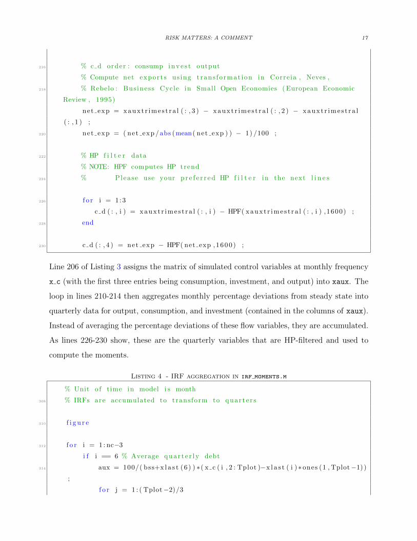
quarterly output, consumption, and investment. The formula they end up using is:10
(1) NXt −NX = Yt − Ct − It ,
where hats denote percentage deviations from the deterministic steady state and bars denote
steady state values, that is:
(2) Yt =Yt − YY
, Ct =Ct − CC
, It =It − II
.
The correct formula should have weighted the percentage deviations of output, consump-
tion, and investment by their respective steady state values:
(3) NXt −NX = Y Yt − CCt − I It .
Table 5 reports the volatility and cyclicality of net exports reported in FGRU and the
volatility and cyclicality of net exports when the time aggregation error and the error in
the computation of net exports are corrected but the structural parameters are kept at the
values calibrated in FGRU. There are two main differences between the results reported by
FGRU and the results in the corrected model.11 First, net exports turn from approximately
acyclical in FGRU to procyclical in the corrected model. The procyclicality of net exports
in the corrected model contrasts with mostly countercyclical net exports in the data.12 The
reason why net exports become procyclical when the computation of net exports is corrected
is that equation (3) puts a relatively larger weight on output fluctuations than equation (1)
due to output in steady state being greater than both consumption and investment.13 This
increase in the weight of the “output component” of net exports mechanically increases the
comovement of net exports with output and hence increases the procyclicality.
10See Appendix A.A3 for details.11The weighting issue also affects the current account implications after risk shocks reported in Figure 6
of FGRU. An updated version of the figure can be found in Appendix B.12Explaining this behavior has motivated prominent papers arguing for the importance of permanent
TFP shocks (e.g. Aguiar and Gopinath, 2007) and financial frictions (e.g. Garcıa-Cicco, Pancrazi and Uribe,2010). Andrea Raffo (2008) has argued that GHH-preferences might be instrumental in getting the correctcorrelation. Adopting the latter may be a way to improve the model fit of FGRU.
13In equation (1) all three components entered with an equal weight of 1, while equation (3) in the FGRU-model implies relative weights of 1, 0.84, and 0.13, for output, consumption, and investment, respectively.

RISK MATTERS: A COMMENT 9
Table 5—Net Exports Keeping the Structural Parameters at the Values Calibrated in
FGRU
Argentina Ecuador
FGRU TA TA+NX Data FGRU TA TA+NX Data
ρNX,Y 0.05 0.05 0.43 -0.76 -0.04 -0.04 0.24 -0.60σNX/σY 0.48 1.43 1.63 0.39 1.77 9.15 1.38 0.39
Venezuela Brazil
FGRU TA TA+NX Data FGRU TA TA+NX Data
ρNX,Y -0.10 -0.10 0.47 -0.11 0.18 0.17 0.78 -0.26σNX/σY 1.60 13.33 1.87 0.18 0.60 1.95 3.87 0.18
Note: first and fifth column: moments reported in FGRU. Second and sixth column: moments obtainedusing the FGRU simulation, but correcting the time aggregation (TA). Third and seventh column: momentsobtained using the FGRU simulation, but correcting the time aggregation and net export computation(TA+NX). Fourth and eighth column: moments obtained from HP-filtered data. Simulations are conductedwith 200 repetitions of 96 periods using the FGRU pruning scheme. For Argentina, the same set of pseudo-random numbers as in FGRU was used, while the simulation for the other countries had to rely on a differentpseudo-random number generator seed.
The second main difference between the results reported by FGRU and the results in the
corrected model is that the corrected model predicts a different volatility of net exports
(see Table 5). To understand the source of this difference, it is useful to start with the
benchmark case of Argentina. The relative volatility of net exports reported in FGRU is
0.48. Correcting time aggregation, the relative net export volatility increases by a factor of
three to 1.43, because the time aggregation error only affects output volatility (FGRU obtain
the volatility of net exports directly at quarterly frequency). Correcting the computation of
net exports leads to a minor further change in relative volatility. As a result, the corrected
relative volatility for the benchmark case of Argentina is approximately 3.4 times the value
reported in FGRU.
From Table 5 it can also be seen that for Ecuador, Venezuela, and Brazil, the difference
between the corrected relative volatility of net exports and the relative volatility reported
in FGRU is sometimes larger than for the benchmark case of Argentina and sometimes
smaller. The reason turns out to be the poor numerical convergence behavior of FGRU’s
measure of net export volatility. Because net exports can be negative, instead of using a
log-linear approximation, FGRU use the Isabel Correia, Joao C. Neves and Sergio Rebelo

10
1000 2000 3000 4000 5000 6000 7000 8000 9000 100000
1
2
3
4
5
Data: 0.39
σNX
/σY
Ave
rage
ove
r R
ep.
1.63
Figure 2. Convergence Behavior of the Relative Net Export Volatility Statistic
Note: relative volatility of net exports to output σNX/σY for the case of Argentina. Net exports transformedto percentage deviations using the Correia, Neves and Rebelo (1995)-approximation. The blue solid lineshows the mean standard deviation (y-axis) over the up to 10,000 samples (x-axis) of simulating 96 monthsof data. The black dashed dotted line shows the actual data moments. The data are based on the correctedaggregation and net export computation. The black arrow indicates the value after 200 replications.
(1995)-approximation of the net exports
(4) NXt ≡NXt
|mean(NXt)|− 1 .
This formula takes the percentage deviations from the absolute value of the mean in order
to preserve the sign.14 If the mean of net exports is close to 0, this can have drawbacks in
short simulations where the mean is imprecisely estimated.
This issue is illustrated in Figure 2. On the vertical axis the figure displays the volatility
of net exports relative to the volatility of output for the benchmark case of Argentina (blue
solid line), computed with the Correia, Neves and Rebelo (1995)-approximation as in FGRU
but correcting the time aggregation error affecting output volatility and the error in the
computation of net exports. The horizontal axis displays the number of simulation repetitions
over which the relative volatility has been computed. As in FGRU, each repetition is based
on a simulation of 96 time periods. The black arrow marks 200 simulations, which is the
number of simulation repetitions that FGRU use to obtain the predicted relative volatility
14Although this expression is already in the same units as output deviations from steady state, FGRUadditionally divide by a factor of 100. Thus, the relative volatility of net exports, σnx/σy is not 0.39 forArgentinean data and 0.48 for the model as reported in FGRU, but 39 and 48, respectively. Subsequently,we report the values in the form originally reported in FGRU.
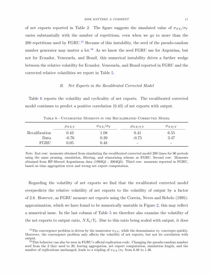
RISK MATTERS: A COMMENT 11
of net exports reported in Table 2. The figure suggests the simulated value of σNX/σY
varies substantially with the number of repetitions, even when we go to more than the
200 repetitions used by FGRU.15 Because of this instability, the seed of the pseudo-random
number generator may matter a lot.16 As we know the seed FGRU use for Argentina, but
not for Ecuador, Venezuela, and Brazil, this numerical instability drives a further wedge
between the relative volatility for Ecuador, Venezuela, and Brazil reported in FGRU and the
corrected relative volatilities we report in Table 5.
B. Net Exports in the Recalibrated Corrected Model
Table 6 reports the volatility and cyclicality of net exports. The recalibrated corrected
model continues to predict a positive correlation (0.43) of net exports with output.
Table 6—Untargeted Moments in the Recalibrated Corrected Model
ρNX,Y σNX/σY ρNX/Y,Y σNX/Y
Recalibration 0.43 1.08 0.41 6.55Data -0.76 0.39 -0.75 3.47
FGRU 0.05 0.48 - -
Note: first row: moments obtained from simulating the recalibrated corrected model 200 times for 96 periodsusing the same pruning, simulation, filtering, and winsorizing scheme as FGRU. Second row: Momentsobtained from HP-filtered Argentinean data (1993Q1 - 2004Q3). Third row: moments reported in FGRU,based on time aggregation error and wrong net export computation.
Regarding the volatility of net exports we find that the recalibrated corrected model
overpredicts the relative volatility of net exports to the volatility of output by a factor
of 2.8. However, as FGRU measure net exports using the Correia, Neves and Rebelo (1995)-
approximation, which we have found to be numerically unstable in Figure 2, this may reflect
a numerical issue. In the last column of Table 5 we therefore also examine the volatility of
the net exports to output ratio, NXt/Yt. Due to this ratio being scaled with output, it does
15The convergence problem is driven by the numerator σNX , while the denominator σY converges quickly.Moreover, the convergence problem only affects the volatility of net exports, but not its correlation withoutput.
16This behavior can also be seen in FGRU’s official replication code. Changing the pseudo-random numberseed from the 2 they used to 20, leaving aggregation, net export computation, simulation length, and thenumber of replications unchanged, leads to a tripling of σNX/σY from 0.48 to 1.46.
12
not suffer from the same division by (almost) zero problem.17 It can be seen that with this
measure of the volatility of net exports, the model prediction is closer to the data than with
the Correia, Neves and Rebelo (1995)-measure used by FGRU. But the predicted volatility is
still almost twice the volatility of the net exports to output ratio in the data. From columns
1 and 3 in Table 6 it can be seen that for the cyclical properties of net exports it does not
matter much which measure of net exports is used.
III. Conclusion
FGRU find that risk shocks have important effects on aggregate variables and might con-
tribute to explaining the current account movements of small open developing economies.
We noted an error in the time aggregation of flow variables that results in the calibrated
model not matching the targeted data moments. Correcting this error and recalibrating the
model to fit the volatilities of output, consumption, and investment, we find that the peak
effect of a risk shock on output increases by 63 percent. The business cycle contribution of
volatility shocks also increases by more than a factor of two.
We also pointed to a weighting error in the net export computation that leads to reported
acyclical net exports when net exports are actually procyclical in the corrected model. We
found that net exports continued to be procyclical in the recalibrated model, thus being at
odds with one of the most robust stylized facts in emerging markets business cycles.
REFERENCES
Adjemian, Stephane, Houtan Bastani, Frederic Karame, Michel Juillard, Junior
Maih, Ferhat Mihoubi, George Perendia, Johannes Pfeifer, Marco Ratto, and
Sebastien Villemot. 2011. “Dynare: reference manual version 4.” CEPREMAP Dynare
Working Papers 1.
Aguiar, Mark, and Gita Gopinath. 2007. “Emerging market business cycles: the cycle
is the trend.” Journal of Political Economy, 115: 69–102.
17Appendix E documents the better convergence behavior of this measure. Using one long simulationfor the Correia, Neves and Rebelo (1995)-approximation instead of averaging over many short ones is noalternative. It does not allow for capturing small sample biases potentially present in the data and, due tothe particular pruning scheme and simulation scheme used in FGRU, leads to results that are not comparableto the short simulations. See Appendix D for details.
RISK MATTERS: A COMMENT 13
Andreasen, Martin M. 2012. “An estimated DSGE model: explaining variation in nominal
term premia, real term premia, and inflation risk premia.” European Economic Review,
56: 1656–1674.
Andreasen, Martin M., Jesus Fernandez-Villaverde, and Juan F. Rubio-Ramırez.
2013. “The pruned state-space system for non-linear DSGE models: theory and empirical
applications.” NBER Working Papers 18983.
Backus, David K., Patrick J. Kehoe, and Finn E. Kydland. 1992. “International
real business cycles.” Journal of Political Economy, 100(4): 745–75.
Baskaya, Yusuf Soner, Timur Hulagu, and Hande Kusuk. 2013. “Oil price uncer-
tainty in a small open economy.” IMF Economic Review, 61(1): 168–198.
Basu, Susanto, and Brent Bundick. 2012. “Uncertainty shocks in a model of effective
demand.” NBER Working Papers 18420.
Born, Benjamin, and Johannes Pfeifer. 2013. “Policy risk and the business cycle.”
CESifo Working Paper Series 4336.
Christiano, Lawrence J., Martin Eichenbaum, and Charles L. Evans. 2005. “Nom-
inal rigidities and the dynamic effects of a shock to monetary policy.” Journal of Political
Economy, 113(1): 1–45.
Correia, Isabel, Joao C. Neves, and Sergio Rebelo. 1995. “Business cycles in a small
open economy.” European Economic Review, 39(6): 1089–1113.
Den Haan, Wouter J., and Joris De Wind. 2012. “Nonlinear and stable perturbation-
based approximations.” Journal of Economic Dynamics and Control, 36(10): 1477–1497.
Fernandez-Villaverde, Jesus, Pablo A. Guerron-Quintana, Juan F. Rubio-
Ramırez, and Martın Uribe. 2011. “Risk matters: the real effects of volatility shocks.”
American Economic Review, 101(6): 2530–61.
Fernandez-Villaverde, Jesus, Pablo A. Guerron-Quintana, Keith Kuester, and
Juan F. Rubio-Ramırez. 2012. “Fiscal volatility shocks and economic activity.” Uni-
versity of Pennsylvania Mimeo.
14
Garcıa-Cicco, Javier, Roberto Pancrazi, and Martın Uribe. 2010. “Real business
cycles in emerging countries?” American Economic Review, 100(5): 2510–31.
Juillard, Michel, and Ondra Kamenik. 2005. “Solving SDGE models: approximation
about the stochastic steady state.” Computing in Economics and Finance 106.
Kim, Jinill, Sunghyun Kim, Ernst Schaumburg, and Christopher A. Sims. 2008.
“Calculating and using second order accurate solutions of discrete time dynamic equilib-
rium models.” Journal of Economic Dynamics and Control, 32(11): 3397 – 3414.
Koop, Gary, M. Hashem Pesaran, and Simon M. Potter. 1996. “Impulse response
analysis in nonlinear multivariate models.” Journal of Econometrics, 74(1): 119–147.
Lan, Hong, and Alexander Meyer-Gohde. 2013a. “Decomposing risk in dynamic
stochastic general equilibrium.” SFB 649 Discussion Papers 22.
Lan, Hong, and Alexander Meyer-Gohde. 2013b. “Pruning in perturbation DSGE
models - guidance from nonlinear moving average approximations.” SFB 649 Discussion
Papers 24.
Neumeyer, Pablo A., and Fabrizio Perri. 2005. “Business cycles in emerging economies:
the role of interest rates.” Journal of Monetary Economics, 52(2): 345–380.
Plante, Michael, and Nora Traum. 2012. “Time-varying oil price volatility and macroe-
conomic aggregates.” Caepr Working Papers 2012-002.
Raffo, Andrea. 2008. “Net exports, consumption volatility and international business cycle
models.” Journal of International Economics, 75(1): 14 – 29.
Reinhart, Carmen M., and Kenneth Rogoff. 2009. This time is different: eight cen-
turies of financial folly. Princeton University Press.
Uribe, Martın, and Vivian Z. Yue. 2006. “Country spreads and emerging countries:
who drives whom?” Journal of International Economics, 69(1): 6–36.
RISK MATTERS: A COMMENT 15
Technical Appendix - For Online Publication
Appendix A documents the coding issues in the Matlab implementation of the model sim-
ulation in more detail by showing the associated computer code of the Fernandez-Villaverde
et al. (2011) (FGRU) replication files posted at http://www.aeaweb.org/articles.php?
doi=10.1257/aer.101.6.2530. FGRU calibrate their model at monthly frequency, per-
form a variable substitution to obtain a log-linearization, and use third-order perturbation
techniques to simulate the model. We make use of the third order perturbation capacities
of Dynare (Stephane Adjemian, Houtan Bastani, Frederic Karame, Michel Juillard, Junior
Maih, Ferhat Mihoubi, George Perendia, Johannes Pfeifer, Marco Ratto and Sebastien Ville-
mot, 2011) to simulate the model.18 Appendix B presents the corrected version of Figure
6 in FGRU. Appendices C and D document the simulation and pruning schemes used for
IRF generation and moment computation. Appendix E compares the numerical convergence
behavior of the standard deviation of the Correia, Neves and Rebelo (1995)-approximation
and of the net export to output ratio. Appendix F compares the deterministic steady state,
the EMAS, and the ergodic mean.
A. The Coding Issues in the Published Replication Files
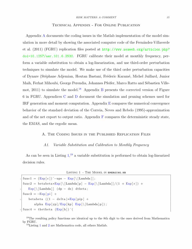
A1. Variable Substitution and Calibration to Monthly Frequency
As can be seen in Listing 1,19 a variable substitution is performed to obtain log-linearized
decision rules.
Listing 1 - The Model in emerging.nb
1 func1 = (Exp [ c ] ) ˆ−ups − Exp [ \ [ Lambda ] ] ;
func2 = betabeta ∗Exp [ \ [ Lambda ] p ] − Exp [ \ [ Lambda ] ] / ( 1 + Exp [ r ] ) +
3 Exp [ \ [ Lambda ] ] (dp − ds ) dtheta ;
func3 = −Exp [ p i ] +
5 betabeta ( (1 − d e l t a ) ∗Exp [ pip ] +
alpha Exp [ yp ] / Exp [ kp ] Exp [ \ [ Lambda ] p ] ) ;
7 func4 = thetheta (Exp [ h ] ) ˆ(
18The resulting policy functions are identical up to the 8th digit to the ones derived from Mathematicaby FGRU.
19Listing 1 and 2 are Mathematica code, all others Matlab.
16
omega + 1) − (1 − alpha ) Exp [ y ] Exp [ \ [ Lambda ] ] ;
9 func5 = −Exp [ \ [ Lambda ] ] +
Exp [ p i ] (1 − phi /2 (Exp [ i n v e s t ] / Exp [ i n v e s t l a g ] − 1) ˆ2 −11 phi Exp [ i n v e s t ] /
Exp [ i n v e s t l a g ] (Exp [ i n v e s t ] / Exp [ i n v e s t l a g ] − 1) ) +
13 betabeta ∗Exp [ pip ] phi (Exp [ inve s tp ] /
15 Exp [ i n v e s t ] ) ˆ2 (Exp [ inve s tp ] / Exp [ i n v e s t ] − 1) ;
func6 = Exp [ y ] − (Exp [ k ] ) ˆ alpha (Exp [ g ] Exp [ h ] ) ˆ(1 − alpha ) ;
17 func8 = dp/(1 + Exp [ r ] ) − d + Exp [ y ] − Exp [ c ] −Exp [ i n v e s t ] − (dp − ds ) ˆ2 dtheta /2 ;
19 func9 = Exp [ r ] − Exp [ r s ] − er − etb ;
func7 = −Exp [ kp ] + (1 − d e l t a ) Exp [
21 k ] + (1 − phi /2 (Exp [ i n v e s t ] / Exp [ i n v e s t l a g ] − 1) ˆ2) Exp [ i n v e s t ] ;
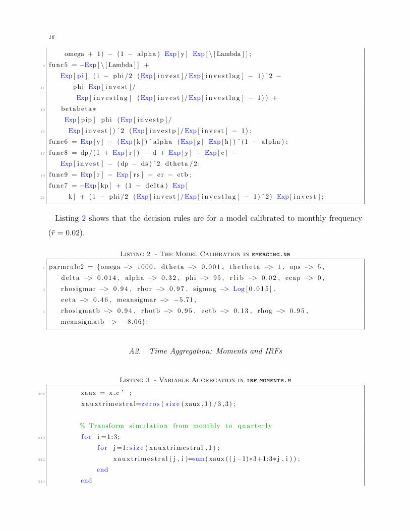
Listing 2 shows that the decision rules are for a model calibrated to monthly frequency
(r = 0.02).
Listing 2 - The Model Calibration in emerging.nb
1 parmrule2 = omega −> 1000 , dtheta −> 0 .001 , thetheta −> 1 , ups −> 5 ,
d e l t a −> 0 .014 , alpha −> 0 . 32 , phi −> 95 , r l i b −> 0 . 02 , ecap −> 0 ,
3 rhosigmar −> 0 . 94 , rhor −> 0 . 97 , sigmag −> Log [ 0 . 0 1 5 ] ,
ee ta −> 0 . 46 , meansigmar −> −5.71 ,
5 rhosigmatb −> 0 . 94 , rhotb −> 0 . 95 , eetb −> 0 . 13 , rhog −> 0 . 95 ,
meansigmatb −> −8.06 ;
A2. Time Aggregation: Moments and IRFs
Listing 3 - Variable Aggregation in irf moments.m
206 xaux = x c ’ ;
xauxt r imes t ra l=ze ro s ( s i z e ( xaux , 1 ) /3 ,3) ;
% Transform s imu la t i on from monthly to q u a r t e r l y
210 f o r i =1:3 ;
f o r j =1: s i z e ( xauxtr imest ra l , 1 ) ;
212 xauxt r imes t ra l ( j , i )=sum( xaux ( ( j−1)∗3+1:3∗ j , i ) ) ;
end
214 end
RISK MATTERS: A COMMENT 17
216 % c d order : consump i n v e s t output
% Compute net export s us ing t rans fo rmat ion in Corre ia , Neves ,
218 % Rebelo : Bus iness Cycle in Small Open Economies ( European Economic
Review , 1995)
net exp = xauxt r imes t ra l ( : , 3 ) − xauxt r imes t ra l ( : , 2 ) − xauxt r imes t ra l
( : , 1 ) ;
220 net exp = ( net exp /abs (mean( net exp ) ) − 1) /100 ;
222 % HP f i l t e r data
% NOTE: HPF computes HP trend
224 % Please use your p r e f e r r e d HP f i l t e r in the next l i n e s
226 f o r i = 1 :3
c d ( : , i ) = xauxt r imes t ra l ( : , i ) − HPF( xauxt r imes t ra l ( : , i ) ,1600) ;
228 end
230 c d ( : , 4 ) = net exp − HPF( net exp ,1600 ) ;
Line 206 of Listing 3 assigns the matrix of simulated control variables at monthly frequency
x c (with the first three entries being consumption, investment, and output) into xaux. The
loop in lines 210-214 then aggregates monthly percentage deviations from steady state into
quarterly data for output, consumption, and investment (contained in the columns of xaux).
Instead of averaging the percentage deviations of these flow variables, they are accumulated.
As lines 226-230 show, these are the quarterly variables that are HP-filtered and used to
compute the moments.
Listing 4 - IRF aggregation in irf moments.m
% Unit o f time in model i s month
308 % IRFs are accumulated to trans form to quar t e r s
310 f i g u r e
312 f o r i = 1 : nc−3
i f i == 6 % Average q u a r t e r l y debt
314 aux = 100/( bss+x l a s t (6 ) ) ∗( x c ( i , 2 : Tplot )−x l a s t ( i ) ∗ ones (1 , Tplot−1) )
;
f o r j = 1 : ( Tplot−2)/3

18
316 argenq ( i , j ) = sum( aux ( ( j−1)∗3+1:3∗ j ) ) ;
end
318 subplot (3 , 2 , i ) ; p l o t ( 0 : ( Tplot−2)/3−1, argenq ( i , : ) /3 , ’ LineWidth ’
, 1 . 5 ) ; a x i s t i g h t ; g r i d on
t i t l e ( varnm( i , : ) , ’ f o n t s i z e ’ , 13) ;
320 e l s e i f i == 5 % Annualized i n t e r e s t r a t e
aux = 10000∗ x s ( 8 , 2 : Tplot ) ;
322 f o r j = 1 : ( Tplot−2)/3
argenq ( i , j ) = sum( aux ( ( j−1)∗3+1:3∗ j ) ) ;
324 end
subplot (3 , 2 , i ) ; p l o t ( 0 : ( Tplot−2)/3−1 ,12∗ argenq ( i , : ) /3 , ’ LineWidth ’
, 1 . 5 ) ; a x i s t i g h t ; g r i d on
326 t i t l e ( varnm( i , : ) , ’ f o n t s i z e ’ , 13) ;
e l s e
328 aux = 100∗( x c ( i , 2 : Tplot )−x l a s t ( i ) ∗ ones (1 , Tplot−1) ) ;
f o r j = 1 : ( Tplot−2)/3
330 argenq ( i , j ) = sum( aux ( ( j−1)∗3+1:3∗ j ) ) ;
end
332 subplot (3 , 2 , i ) ; p l o t ( 0 : ( Tplot−2)/3−1, argenq ( i , : ) , ’ LineWidth ’ , 1 . 5 )
; a x i s t i g h t ; g r i d on
t i t l e ( varnm( i , : ) , ’ f o n t s i z e ’ , 13) ;
334 end
end
Listing 4 shows the time aggregation from monthly model IRFs to the quarterly IRFs
reported in FGRU. As can be seen in lines 313-319, the stock of debt is first expressed as
a percentage deviation from the EMAS (line 314) and then aggregated by taking the mean
response over three subsequent quarters: the subsequent three months are summed up (line
316) and then divided by 3 before plotting (line 318). Similarly, lines 321-325 take the
interest rate spread εr,t, average it and multiply it by 12× 100× 100 = 120,000 to transform
it into annualized basis points.
Line 328 computes the difference between the log of the monthly model variables (output,
consumption, investment, and hours) and the EMAS times 100, which has the interpretation
of a percentage deviation. Lines 329 to 331 sum up the monthly percentage deviations over
the quarter, before line 332 plots them without dividing by three as was the case in line 318.
As a result, the percentage deviations from steady state of the flow variables like output,
RISK MATTERS: A COMMENT 19
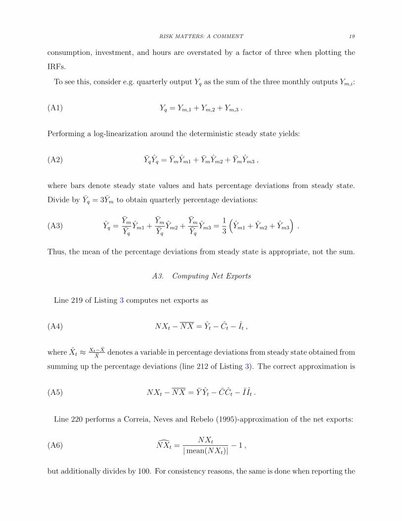
consumption, investment, and hours are overstated by a factor of three when plotting the
IRFs.
To see this, consider e.g. quarterly output Yq as the sum of the three monthly outputs Ym,i:
(A1) Yq = Ym,1 + Ym,2 + Ym,3 .
Performing a log-linearization around the deterministic steady state yields:
(A2) YqYq = YmYm1 + YmYm2 + YmYm3 ,
where bars denote steady state values and hats percentage deviations from steady state.
Divide by Yq = 3Ym to obtain quarterly percentage deviations:
(A3) Yq =YmYqYm1 +
YmYqYm2 +
YmYqYm3 =
1
3
(Ym1 + Ym2 + Ym3
).
Thus, the mean of the percentage deviations from steady state is appropriate, not the sum.
A3. Computing Net Exports
Line 219 of Listing 3 computes net exports as
(A4) NXt −NX = Yt − Ct − It ,
where Xt ≈ Xt−XX
denotes a variable in percentage deviations from steady state obtained from
summing up the percentage deviations (line 212 of Listing 3). The correct approximation is
(A5) NXt −NX = Y Yt − CCt − I It .
Line 220 performs a Correia, Neves and Rebelo (1995)-approximation of the net exports:
(A6) NXt =NXt
|mean(NXt)|− 1 ,
but additionally divides by 100. For consistency reasons, the same is done when reporting the

20
empirical standard deviation (see line 36 of Listing 5). This implies that both the empirical
and theoretical moments for net exports are underreported by a factor of 100 in the paper.
Listing 5 - Net Export display in empirical moments.m
di sp ( ’Moments Argentina : vo l c/ vo l y vo l invt / vo l y vo l net export / vo l y ’ )
36 [ s td ( cd ) std ( id ) std (nd) /100 ]/ std ( yd )
A4. Computing the Net Exports Share
Line 247 of Listing 6 computes the net exports to output share from the national income
accounting identity:
(A7) NXt = Yt − Ct − It = Dt −Dt+1
1 + rt+
ΦD
2
(Dt+1 − D
)2
at the EMAS as
(A8)NX
Y=
[D +
(D − D
)]r−1r
elog(Y )+(log(Y )−log(Y )),
where the respective deviations of the EMAS from the deterministic steady state are stored
in xlast. But in the EMAS D 6= D. Thus, the adjustment cost term in equation (A7) is not
zero. As a consequence, the permanent portfolio holdings costs paid at the EMAS are not
accounted for when computing the net exports required to finance the debt stock. For the
original calibration this coding issue is inconsequential due to the low debt adjustment costs.
But when recalibrating the model, the debt holding costs need to be taken into account as
one cannot know a priori if they are substantial.
Listing 6 - Net-Export Share Calibration in irf moments.m
244 % 2 . 2 . 1 Compute moments in Table 7 , Column M1
246 di sp ( ’ Ratio net export s / output ’ )
( ( bss+x l a s t (6 ) ) ∗( I ra t e −1)/ I r a t e ) /( exp ( adyss+x l a s t (3 ) ) )

RISK MATTERS: A COMMENT 21
B. Figure FGRU6: IRFs Debt/Output, Current Account, Net Exports
Figure 6 in FGRU, reproduced here as Figure B1 due to non-availability of replication
codes, depicts the responses of the debt to output ratio, the current account, and net exports
to a risk shock. 2553FERnándEz-ViLLAVERdE ET AL.: Risk MATTERsVOL. 101 nO. 6
The last row in Figure 5 plots the IRFs in the M2 version of the model. In this row, we plot the IRFs after a one-standard-deviation level shock that is accompanied by a κ− standard deviation shock to volatility. The pattern of the IRFs is qualitatively the same as in the first row. The lesson from this third row is that our results are robust to the correlation between innovations.
We conclude by pointing out two features of our model. First, our results come in a model without working capital, a mechanism often added to improve the perfor-mance of international macro models. As shown in the online Appendix, working capital makes our findings even stronger. Second, we do not have any of the real-option effects of risk emphasized by the literature, for example, when we have irre-versibilities (Bloom 2009). Introducing those effects explicitly is difficult with our perturbation approach because of the nondifferentiability of threshold decision rules created by real-option environments. However, real-option effects would increase the impact of shocks to volatility on investment. Therefore, our results are likely to be a lower bound to the implications of time-varying risk. Bloom, Jaimovich, and Floetotto (2008) explore the real-option effects of volatility shocks in a model calibrated for the US economy, but a more thorough investigation of the interaction between our higher-order terms and real-option effects remains an open question.
Ecuador.—Next, we turn to Ecuador, whose IRFs are plotted in Figure 7. The IRFs are similar to those in the Argentinian case. There is a decline in economic activity with responses qualitatively similar to, although somewhat smaller than, those for Argentina. After a shock to volatility, consumption drops 0.44 percent upon impact, investment 0.66 percent, and debt 0.08 percent. Investment falls for five quarters
Figure 6. IRFs Debt/Output, Current Account, Net Exports
2 4 6 8 10 12 14 16
0.265
0.27
0.275
0.28
0.285
0.29
Debt/output
Current account Net exports
1.5
1
0.5
0
2
1.5
1
0.5
0
2 4 6 8 10 12 14 16 2 4 6 8 10 12 14 16
Figure B1. IRFs Debt/Output, Current Account, Net Exports
Note: Reproduced Figure 6 from Fernandez-Villaverde et al. (2011), p. 2553.
FGRU report the debt to output ratio IRF in that figure not in percentage deviations
from the EMAS, but as the absolute value. Figure B2 displays that the debt to output ratio
dropped from about 0.293 by about 2.9 percentage points to 0.263 after 11 periods. But
this is inconsistent with the FGRU-IRFs in Figure C1, which show that debt dropped by
3.873 percent while output dropped by 0.1907 percent. Thus, the new debt-to-output-ratio
should be up to first order (1−0.03873)D/((1−0.001907)Y ) ≈ 0.963D/Y , i.e. it should drop
by about 3.7 percent (not percentage points). The net export IRF is affected by from the
incorrect weighting used in their computation as shown in section II. Regarding the current
account, FGRU state that it is in “percentage points of [its] ergodic mean”. But this is not
possible for it is defined as CAt = Dt − Dt−1 and thus has ergodic mean zero. Thus, it is
unclear what the lower left panel of Figure B2 depicts.
The left column of Figure B2 shows the corrected version of Figure 6 in FGRU that uses
output to normalize net exports and the current account, giving them the interpretation of
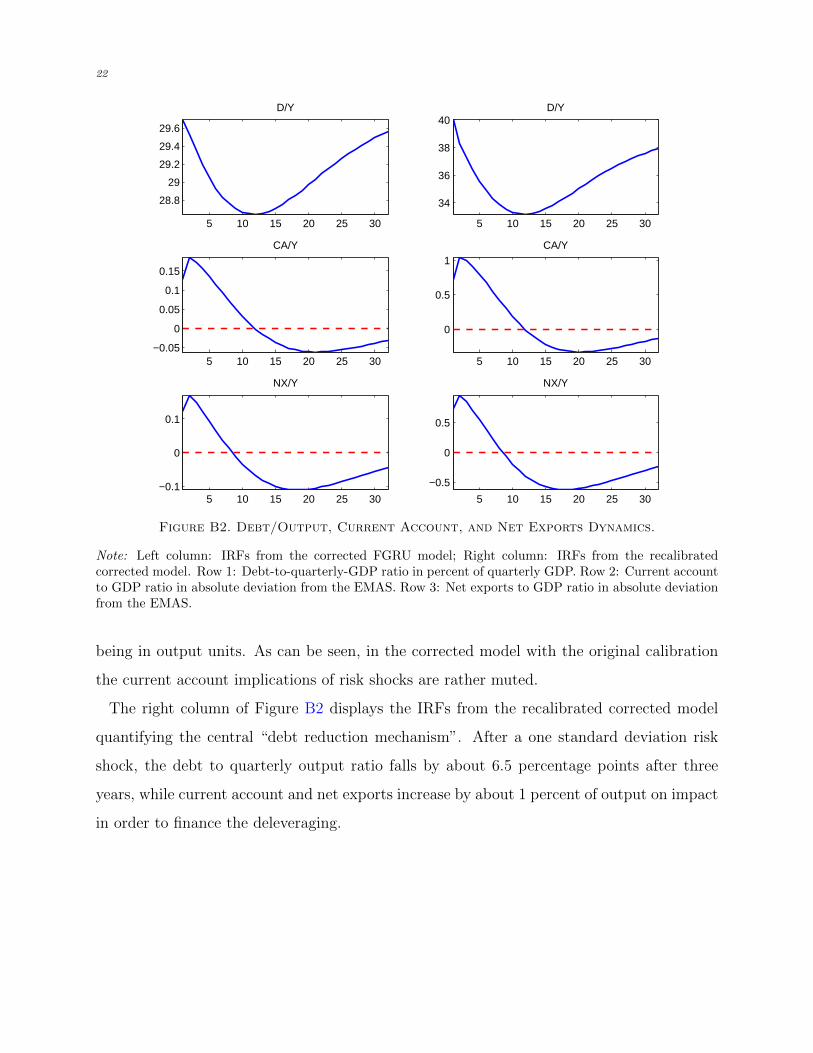
22
5 10 15 20 25 30
28.8
29
29.2
29.4
29.6
D/Y
5 10 15 20 25 30−0.05
0
0.05
0.1
0.15
CA/Y
5 10 15 20 25 30−0.1
0
0.1
NX/Y
5 10 15 20 25 30
34
36
38
40D/Y
5 10 15 20 25 30
0
0.5
1
CA/Y
5 10 15 20 25 30
−0.5
0
0.5
NX/Y
Figure B2. Debt/Output, Current Account, and Net Exports Dynamics.
Note: Left column: IRFs from the corrected FGRU model; Right column: IRFs from the recalibratedcorrected model. Row 1: Debt-to-quarterly-GDP ratio in percent of quarterly GDP. Row 2: Current accountto GDP ratio in absolute deviation from the EMAS. Row 3: Net exports to GDP ratio in absolute deviationfrom the EMAS.
being in output units. As can be seen, in the corrected model with the original calibration
the current account implications of risk shocks are rather muted.
The right column of Figure B2 displays the IRFs from the recalibrated corrected model
quantifying the central “debt reduction mechanism”. After a one standard deviation risk
shock, the debt to quarterly output ratio falls by about 6.5 percentage points after three
years, while current account and net exports increase by about 1 percent of output on impact
in order to finance the deleveraging.

RISK MATTERS: A COMMENT 23
C. IRFs at the Ergodic Mean
C1. IRF Generation
The use of higher-order perturbation techniques to solve the model implies that the model
solution is not linear anymore. Thus, the IRFs will depend on both the sequence of future
shocks, ut, and the point in the state space at which the IRFs are started, i.e. the past
history of shocks, Ωt. To circumvent this problem, Gary Koop, M. Hashem Pesaran and
Simon M. Potter (1996) suggested the concept of Generalized Impulse Response Functions
(GIRFs) that e.g. allow considering “representative” IRFs at the ergodic mean. The GIRF
at time t+ n after a shock ut is given by
(C1) GIRFn (ut,Ωt−1) = E [Yt+n|ut,Ωt−1]− E [Yt+n|Ωt−1] ,
that is, given a point in the state space, the future shock realizations are averaged out.
In contrast, FGRU also condition on future shocks by setting them to 0 when generating
their IRFs and start the IRFs at the EMAS. Denote the future realization of shocks with
Ωfut. FGRU effectively use the definition
IRFn (νt,Ωt) = E[Yt+n|ut,Ωt−1 = . . . , 0 ,Ωfut
t+1 = 0, . . .]
− E[Yt+n|0,Ωt−1 = . . . , 0 ,Ωfut
t+1 = 0, . . .],(C2)
where the expected values can be dropped as everything is deterministic.
This choice of computing the IRFs at the EMAS has two important implications. First,
computing the non-linear IRFs not as the expected difference in responses as in (C1) but
also conditioning on future shocks and setting them to 0, only allows capturing part of the
economic effects of risk shocks. To see this, inspect the particular pruning algorithm20 used
20As first noted in Jinill Kim, Sunghyun Kim, Ernst Schaumburg and Christopher A. Sims (2008), higherorder perturbation solutions tend to explode due to the accumulation of terms of increasing order. Forexample, in a second order approximated solution, the quadratic term at time t will be raised to the powerof two in the quadratic term at t + 1, thus resulting in a quartic term, which will become a term of order8 at t + 2 and so on. As a solution, Kim et al. (2008) proposed “pruning” all terms of higher order, i.e.computing the quadratic term at t + 1 by only squaring the first-order term from time t. This procedure,however, is not easily generalized to third order as there are several potential ways of pruning.
24
in FGRU for IRF-generation.21 Consider a generic model solution of the form
(C3) xt = g(xstatest−1 , ut, σ
),
where xt is an nx× 1 vector of endogenous variables, xstatest−1 is the vector of states contained
in xt,22 ut is an nu × 1 vector of mean zero disturbances, and σ is the perturbation param-
eter. Denote partial derivatives with subscripts. The pruned third order solution for the
endogenous variables’ deviations from their steady state, x3rdt = x3rd
t − x, used by FGRU, is
computed from the recursion
x3rdt =gxx
3rd,statest−1 + guut
+1
2
[gxx(x1st,statest−1 ⊗ x1st,states
t−1
)+ 2gxu
(x1st,statest−1 ⊗ ut
)+ guu (ut ⊗ ut) + gσσσ
2]
+1
6
gxxx
(x1st,statest−1 ⊗ x1st,states
t−1 ⊗ x1st,statest−1
)+ guuu (ut ⊗ ut ⊗ ut)
+3gxxu(x1st,statest−1 ⊗ x1st,states
t−1 ⊗ ut)
+ 3gxuu(x1st,statest−1 ⊗ ut ⊗ ut
)+3gxσσσ
2x1st,statest−1 + 3guσσσ
2ut
(C4)
x1stt =gxx
1st,statest−1 + guut .(C5)
That is, all higher order terms are based on the first-order terms.23 The recursion in equations
(C4)-(C5) is completed by an initial condition24 of:
x3rd0 = x− x(C6)
x1st0 = 0 .(C7)
Because x1st0 = 0 and all higher order terms in equation (C4) are based on it, the effect
21The IRF-pruning scheme differs from the scheme used for simulations, see Appendix D.22We use the Dynare notation that stacks the state transition and observation equations (see Adjemian
et al., 2011).23This choice results in an inferior performance compared to e.g. the pruning scheme by Martin M.
Andreasen, Jesus Fernandez-Villaverde and Juan F. Rubio-Ramırez (2013) that augments the state space tokeep track of first to third order terms and uses the Kronecker product of the first and second order termsto compute the third order term (see Hong Lan and Alexander Meyer-Gohde, 2013b, for more details).
24As shown in Lan and Meyer-Gohde (2013b) there are infinitely many different past shock realizationsthat can lead to being at a particular point in the state-space at time 0, all of them associated with particularvalues for x3rd0 and x1st0 . Equations (C6) to (C7) are consistent with the EMAS in that one particular shockcombination giving rise to these values is the total absence of past shocks.

RISK MATTERS: A COMMENT 25
of the initial condition x − x will mostly be neglected. Equation (C5) effectively is a first-
order policy function, which is known not to react to risk shocks, except for the state σt−1.
Considering (C4), this and the conditioning on all shocks being 0 ∀ t + i, i > 0 implies
that, in the terminology of Hong Lan and Alexander Meyer-Gohde (2013a), only the “risk
adjustment channel” is present (via the constant term 1/2× gσσ × σ2 and the time-varying
risk-adjustment 1/2 × guσσ × σ2 × ut in period t where ut 6= 0). But the difference in
“amplification effects” introduced by (risk) shocks and embedded in the other higher order
terms is totally absent. Thus, the difference in the interaction between the location in the
state space and future shocks, introduced by the risk shock, is not captured.
Second, the IRFs are computed at a particular point in the pruned state space where
agents factor in the uncertainty of the system, but where there has been an infinite absence
of shocks. Due to the absence of shocks and thus of “amplification effects” embedded in the
higher order terms, agents will dare to incur a relatively high amount of debt. As shown
in Table F1, the difference between the EMAS and the unconditional mean amounts to 20
percent.25
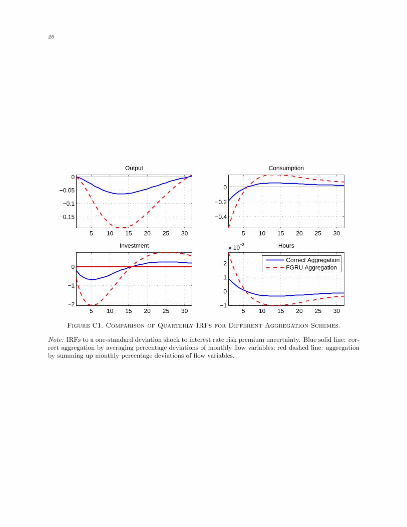
C2. IRF Generation
Figure C1 compares the responses after a one-standard deviation interest rate risk shock
reported in FGRU (red dashed lines) with the responses when the time aggregation error
is corrected (blue solid lines). It can be seen that correcting the time aggregation error
mechanically results in the size of the shock response dropping to one third of the value
reported in FGRU. For example, instead of dropping by 0.19 percent, output falls by a 0.06
percent at its trough.
25An alternative would be to compute GIRFs at the true ergodic mean using the methods proposed inAndreasen, Fernandez-Villaverde and Rubio-Ramırez (2013).
26
5 10 15 20 25 30
−0.15
−0.1
−0.05
0
Output
5 10 15 20 25 30
−0.4
−0.2
0
Consumption
5 10 15 20 25 30−2
−1
0
Investment
5 10 15 20 25 30−1
0
1
2
x 10−3 Hours
Correct AggregationFGRU Aggregation
Figure C1. Comparison of Quarterly IRFs for Different Aggregation Schemes.
Note: IRFs to a one-standard deviation shock to interest rate risk premium uncertainty. Blue solid line: cor-rect aggregation by averaging percentage deviations of monthly flow variables; red dashed line: aggregationby summing up monthly percentage deviations of flow variables.
RISK MATTERS: A COMMENT 27
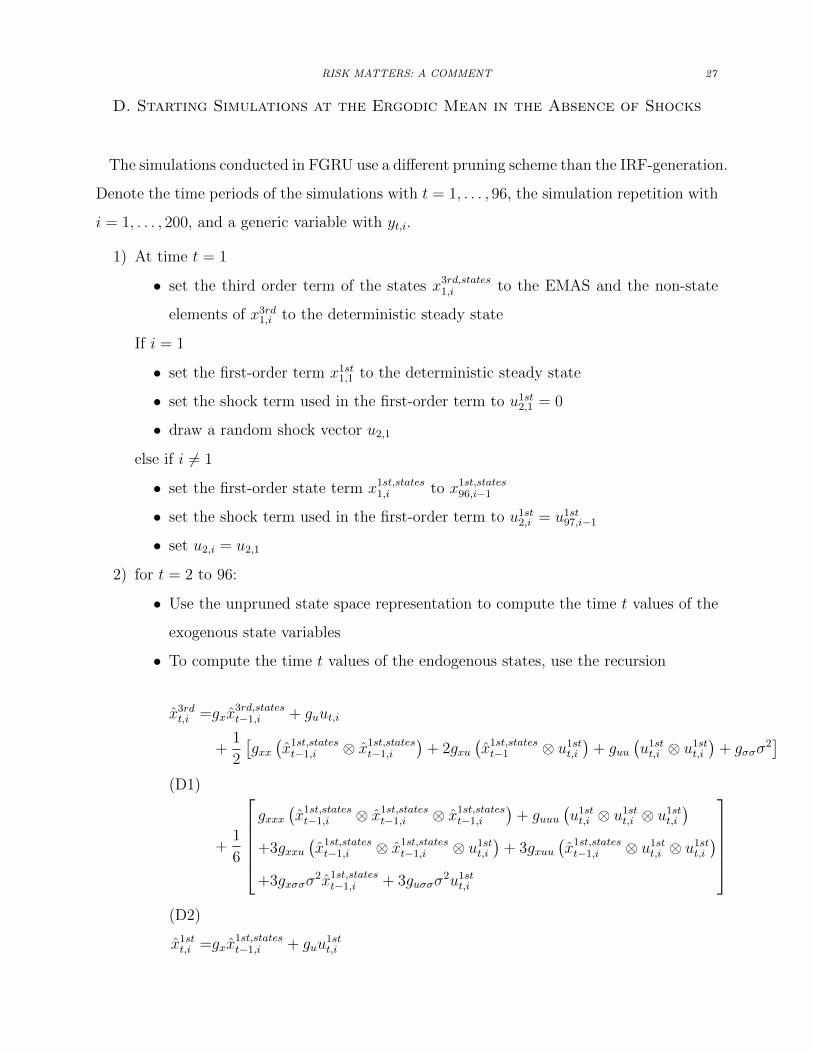
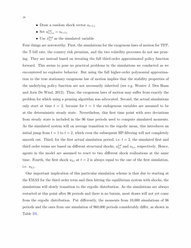
D. Starting Simulations at the Ergodic Mean in the Absence of Shocks
The simulations conducted in FGRU use a different pruning scheme than the IRF-generation.
Denote the time periods of the simulations with t = 1, . . . , 96, the simulation repetition with
i = 1, . . . , 200, and a generic variable with yt,i.
1) At time t = 1
• set the third order term of the states x3rd,states1,i to the EMAS and the non-state
elements of x3rd1,i to the deterministic steady state
If i = 1
• set the first-order term x1st1,1 to the deterministic steady state
• set the shock term used in the first-order term to u1st2,1 = 0
• draw a random shock vector u2,1
else if i 6= 1
• set the first-order state term x1st,states1,i to x1st,states
96,i−1
• set the shock term used in the first-order term to u1st2,i = u1st
97,i−1
• set u2,i = u2,1
2) for t = 2 to 96:
• Use the unpruned state space representation to compute the time t values of the
exogenous state variables
• To compute the time t values of the endogenous states, use the recursion
x3rdt,i =gxx
3rd,statest−1,i + guut,i
+1
2
[gxx(x1st,statest−1,i ⊗ x1st,states
t−1,i
)+ 2gxu
(x1st,statest−1 ⊗ u1st
t,i
)+ guu
(u1stt,i ⊗ u1st
t,i
)+ gσσσ
2]
+1
6
gxxx
(x1st,statest−1,i ⊗ x1st,states
t−1,i ⊗ x1st,statest−1,i
)+ guuu
(u1stt,i ⊗ u1st
t,i ⊗ u1stt,i
)+3gxxu
(x1st,statest−1,i ⊗ x1st,states
t−1,i ⊗ u1stt,i
)+ 3gxuu
(x1st,statest−1,i ⊗ u1st
t,i ⊗ u1stt,i
)+3gxσσσ
2x1st,statest−1,i + 3guσσσ
2u1stt,i
(D1)
x1stt,i =gxx
1st,statest−1,i + guu
1stt,i
(D2)
28
• Draw a random shock vector ut+1,i
• Set u1stt+1,i = ut+1,i
• Use x3rdt,i as the simulated variable
Four things are noteworthy. First, the simulations for the exogenous laws of motion for TFP,
the T-bill rate, the country risk premium, and the two volatility processes do not use prun-
ing. They are instead based on iterating the full third-order approximated policy function
forward. This seems to pose no practical problems in the simulations we conducted as we
encountered no explosive behavior. But using the full higher-order polynomial approxima-
tion to the true stationary exogenous law of motion implies that the stability properties of
the underlying policy function are not necessarily inherited (see e.g. Wouter J. Den Haan
and Joris De Wind, 2012). Thus, the exogenous laws of motion may suffer from exactly the
problem for which using a pruning algorithm was advocated. Second, the actual simulations
only start at time t = 2, because for t = 1 the endogenous variables are assumed to be
at the deterministic steady state. Nevertheless, this first time point with zero deviations
from steady state is included in the 96 time periods used to compute simulated moments.
As the simulated system will on average transition to the ergodic mean, this introduces an
initial jump from t = 1 to t = 2, which even the subsequent HP-filtering will not completely
smooth out. Third, for the first actual simulation period, i.e. t = 2, the simulated first and
third order terms are based on different structural shocks, u1st2,i and u2,i, respectively. Hence,
agents in the model are assumed to react to two different shock realizations at the same
time. Fourth, the first shock u2,i at t = 2 is always equal to the one of the first simulation,
i.e. u2,1.
One important implication of this particular simulation scheme is that due to starting at
the EMAS for the third order term and then hitting the equilibrium system with shocks, the
simulations will slowly transition to the ergodic distribution. As the simulations are always
restarted at this point after 96 periods and there is no burnin, most draws will not yet come
from the ergodic distribution. Put differently, the moments from 10,000 simulations of 96
periods and the ones from one simulation of 960,000 periods considerably differ, as shown in
Table D1.
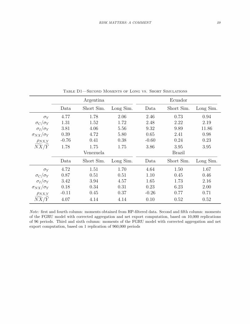
RISK MATTERS: A COMMENT 29
Table D1—Second Moments of Long vs. Short Simulations
Argentina Ecuador
Data Short Sim. Long Sim. Data Short Sim. Long Sim.
σY 4.77 1.78 2.06 2.46 0.73 0.94σC/σY 1.31 1.52 1.72 2.48 2.22 2.19σI/σY 3.81 4.06 5.56 9.32 9.89 11.86
σNX/σY 0.39 4.72 5.80 0.65 2.41 0.98ρNX,Y -0.76 0.41 0.38 -0.60 0.24 0.23
NX/Y 1.78 1.75 1.75 3.86 3.95 3.95Venezuela Brazil
Data Short Sim. Long Sim. Data Short Sim. Long Sim.
σY 4.72 1.51 1.70 4.64 1.50 1.67σC/σY 0.87 0.51 0.51 1.10 0.45 0.46σI/σY 3.42 3.94 4.57 1.65 1.73 2.16
σNX/σY 0.18 0.34 0.31 0.23 6.23 2.00ρNX,Y -0.11 0.45 0.37 -0.26 0.77 0.71
NX/Y 4.07 4.14 4.14 0.10 0.52 0.52
Note: first and fourth column: moments obtained from HP-filtered data. Second and fifth column: momentsof the FGRU model with corrected aggregation and net export computation, based on 10,000 replicationsof 96 periods. Third and sixth column: moments of the FGRU model with corrected aggregation and netexport computation, based on 1 replication of 960,000 periods

30
E. Convergence Behavior of the Net Exports to Output Ratio
1000 2000 3000 4000 5000 6000 7000 8000 9000 100000
0.5
1
1.5
Data: 0.39
σNX
/σY
Ave
rage
ove
r R
ep.
1000 2000 3000 4000 5000 6000 7000 8000 9000 100000
2
4
6
8
Data: 3.47
σNX/Y
Repetitions
Ave
rage
ove
r R
ep.
1.08
6.55
Figure E1. Convergence Behavior of Different Net Export Volatility Statistics in the
Recalibrated Model
Note: top panel: relative volatility of net exports to output σNX/σY . Net exports transformed to percentagedeviations using the Correia, Neves and Rebelo (1995)-approximation. Bottom panel: standard deviation ofthe net exports to output ratio σNX/Y . The blue solid line shows the mean standard deviation (y-axis) overthe up to 10,000 samples (x-axis) of simulating 96 months of data. The black dashed dotted line shows theactual data moments. The data are based on the corrected aggregation and net export computation. Theblack arrow indicates the value after 200 replications.

RISK MATTERS: A COMMENT 31
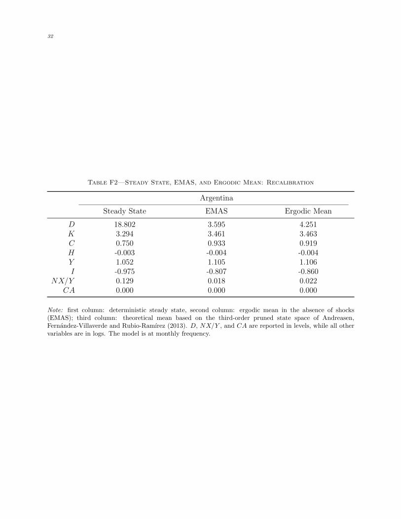
F. Steady State, EMAS, and Ergodic Mean
Table F1—Steady State, EMAS, and Ergodic Mean: FGRU Calibration
Argentina Ecuador
SteadyState
EMAS Erg. Mean SteadyState
EMAS Erg. Mean
D 4.000 2.551 2.090 13.000 12.040 12.072K 3.293 3.287 3.309 3.745 3.757 3.757C 0.878 0.888 0.905 0.945 0.951 0.951H -0.004 -0.004 -0.004 -0.004 -0.004 -0.004Y 1.051 1.049 1.056 1.196 1.200 1.200I -0.975 -0.982 -0.969 -0.523 -0.512 -0.518
NX/Y 0.027 0.018 0.005 0.043 0.039 0.038CA 0.000 0.000 0.000 0.000 0.000 0.000
Venezuela Brazil
SteadyState
EMAS Erg. Mean SteadyState
EMAS Erg. Mean
D 22.000 21.422 21.445 3.000 2.709 2.651K 4.002 4.009 4.010 4.001 4.003 4.005C 0.982 0.985 0.985 1.030 1.031 1.032H -0.004 -0.004 -0.004 -0.004 -0.004 -0.004Y 1.278 1.280 1.280 1.278 1.278 1.279I -0.267 -0.260 -0.265 -0.267 -0.266 -0.265
NX/Y 0.043 0.041 0.041 0.006 0.005 0.005CA 0.000 0.000 -0.000 0.000 0.000 -0.000
Note: first column: deterministic steady state, second column: ergodic mean in the absence of shocks(EMAS); third column: theoretical mean based on the third-order pruned state space of Andreasen,Fernandez-Villaverde and Rubio-Ramırez (2013). D, NX/Y , and CA are reported in levels, while all othervariables are in logs. The model is at monthly frequency.
Table F1 implies that D/Yannual = 2.09/(12 × exp(1.056)) ≈ 0.0606. In the recalibrated
model, D/Yannual = 4.251/(12× exp(1.106)) ≈ 0.1172.
32
Table F2—Steady State, EMAS, and Ergodic Mean: Recalibration
Argentina
Steady State EMAS Ergodic Mean
D 18.802 3.595 4.251K 3.294 3.461 3.463C 0.750 0.933 0.919H -0.003 -0.004 -0.004Y 1.052 1.105 1.106I -0.975 -0.807 -0.860
NX/Y 0.129 0.018 0.022CA 0.000 0.000 0.000
Note: first column: deterministic steady state, second column: ergodic mean in the absence of shocks(EMAS); third column: theoretical mean based on the third-order pruned state space of Andreasen,Fernandez-Villaverde and Rubio-Ramırez (2013). D, NX/Y , and CA are reported in levels, while all othervariables are in logs. The model is at monthly frequency.