Risk Optimization for Hybrid Pension Plans with

ARMA and GARCH Investment Returns

Ashwag ALzahrani

A Project

for The Department of

Mathematics and Statistics

Presented in Partial Fulfillment of the Requirements

for the Degree of Master of Science (Mathematics) at

Concordia University

Montreal, Quebec, Canada

May 2016

c© Ashwag ALzahrani, 2016

CONCORDIA UNIVERSITY

School of Graduate Studies

This is to certify that the project prepared

By: Ashwag ALzahrani

Entitled: Risk Optimization for Hybrid Pension Plans with ARMA and

GARCH Investment Returns

and submitted in partial fulfillment of the requirements for the degree of

Master of Science (Mathematics)

complies with the regulations of the University and meets the accepted standards with

respect to originality and quality.

iii

Abstract

The use of time series models in general, and conditional processes, in particular

for modelling returns on investment, have been considered recently for pension plan

funding. In this project, ARMA and GARCH models are applied to the rate of return

of a hybrid pension plan. The first and second moments of the fund, contributions,

and benefits are derived under both models. The aggregate risk and the optimal

spread period of amortization are studied under different risk measures; Value at Risk,

Coefficient of Variation, and Variance. All evaluations are done over finite as well

as infinite time horizons. Finally, numerical illustrations under different investment

strategies as well as different valuation interest Rates are proposed under GARCH

model.

Keywords: Hybrid Pension Designs, Funding Methods, Risk Sharing, Yield Rate,

ARMA(1, 1), GARCH(1, 1), Aggregate Risk, VaR, TVaR.

iv

In memory of my parents

Febuary 2013

April 2014

v

“Nothing is impossible, the word itself says ‘I’m possible’ ”

Audrey Hepburn

vi

Acknowledgments

I would like to express my deep gratitude and appreciation to my deceased parents;

Saeed ALzahrani and Fatimah ALzahrani; who supported my dreams to complete

my Masters degree. Without their encouragement I would have not made it this

far. I dedicate my work to them although they are not here to see the fruit of their labor.

I also would like to acknowledge my supervisor Jose Garrido for the support and

valuable advice that he has provided over the past few years. The amount of knowledge

that he shared with me during my reaserch work were more than useful, and it will

remain a constant encouragement for years to come.

I also thank Prof. Ricardas Zitikis and Dr. Maciej Augustyniak for helping me in

this project. Thank you, Omar Alzahrani, for providing the information that was the

foundation for my work. The advice that he provided was of great value that assisted

me in completing this project. All thanks goes out to friends and family that provided

support to me through out the years while in Canada.

Thanks for the monetary support that was provided by the Goverment of Saudi

Arabia through Ministry of Education as well as the Saudi Cultural Bureau.

vii

Contents

List of Tables xi

List of Figures xii

1 Introduction 1

1.1 Defined Benefit (DB) Plan . . . . . . . . . . . . . . . . . . . . . . . . 1

1.2 Defined Contribution (DC) Plan . . . . . . . . . . . . . . . . . . . . . 1

1.3 Hybrid Plan . . . . . . . . . . . . . . . . . . . . . . . . . . . . . . . . 2

1.3.1 Hybrid Pension Designs . . . . . . . . . . . . . . . . . . . . . 2

1.4 Types of Risks In Pension Plans . . . . . . . . . . . . . . . . . . . . . 4

1.5 Actuarial Funding Methods . . . . . . . . . . . . . . . . . . . . . . . 6

1.6 Two Case Studies . . . . . . . . . . . . . . . . . . . . . . . . . . . . . 7

1.6.1 Pension Design In Saudi Arabia . . . . . . . . . . . . . . . . . 8

1.6.2 Pension Plan In Canada . . . . . . . . . . . . . . . . . . . . . 13

2 Risk Measurement 19

2.1 Coherent Risk Measures . . . . . . . . . . . . . . . . . . . . . . . . . 19

2.2 Value at Risk (VaR) . . . . . . . . . . . . . . . . . . . . . . . . . . . 21

2.3 Conditional Value at Risk (CVaR) . . . . . . . . . . . . . . . . . . . . 22

3 Model Structure and Assumptions 24

3.1 Risk Sharing in a Hybrid Pension Plan . . . . . . . . . . . . . . . . . 24

3.2 Modeling a Hybrid Plan . . . . . . . . . . . . . . . . . . . . . . . . . 25

3.2.1 Assumptions . . . . . . . . . . . . . . . . . . . . . . . . . . . . 25

viii

3.2.2 Notation . . . . . . . . . . . . . . . . . . . . . . . . . . . . . . 26

4 Models for the Return on Investment 29

4.1 Rate of Return it . . . . . . . . . . . . . . . . . . . . . . . . . . . . . 30

4.2 Autoregressive Moving Average (ARMA) Model . . . . . . . . . . . 30

4.2.1 Marginal Moments under ARMA(1, 1) . . . . . . . . . . . . . 32

4.3 Generalized Autoregressive Conditional

Heteroskedasticity (GARCH) . . . . . . . . . . . . . . . . . . . . . . 34

4.3.1 Conditional Moments of the GARCH(1, 1) Model . . . . . . 41

4.3.2 Marginal Moments of the GARCH(1, 1) Model . . . . . . . . 42

4.4 Long-Memory Models . . . . . . . . . . . . . . . . . . . . . . . . . . . 44

4.4.1 Autoregressive Fractionally Integrated Moving Average Model

(ARFIMA) . . . . . . . . . . . . . . . . . . . . . . . . . . . . 45

4.4.2 Fractionally Integrated Generalized Autoregressive

Conditional Heteroscedastic (FIGARCH) . . . . . . . . . . . 46

5 Risk Measurement under Hybrid Pension Plan 49

5.1 Moments of the Fund, Contribution, and Benefit Levels . . . . . . . . 50

5.1.1 Moments of the Fund Level under ARMA(1, 1) . . . . . . . . 51

5.1.2 Moments of the Fund Level under GARCH(1, 1) . . . . . . . 55

5.1.3 Comments on the Moments of Cash Flows . . . . . . . . . . . 57

5.2 Aggregate Risk and Optimal Spread Parameter . . . . . . . . . . . . 59

5.2.1 Analyzing the Optimal Spread Parameter . . . . . . . . . . . 60

5.2.2 Aggregate Risk under Variance, Coefficient of Variation, and

Value at Risk . . . . . . . . . . . . . . . . . . . . . . . . . . . 61

5.2.3 Comments on the Aggregate Risk and Spread Parameter . . . 64

5.3 Numerical Illustration . . . . . . . . . . . . . . . . . . . . . . . . . . 65

5.3.1 Varying Spread Periods . . . . . . . . . . . . . . . . . . . . . . 66

5.3.2 Varying Risk Measures and Spread Periods . . . . . . . . . . . 70

5.3.3 Varying Investment Strategies and Spread Periods . . . . . . . 73

5.3.4 Varying Valuation Interest Rates and Spread Periods . . . . . 75

ix

5.3.5 Varying Valuation Time and Spread Periods . . . . . . . . . . 78

6 Conclusion 79

6.1 Future Work . . . . . . . . . . . . . . . . . . . . . . . . . . . . . . . . 80

Bibliography 82

A Derivations 88

A.1 The Derivation of Equation (4.2) . . . . . . . . . . . . . . . . . . . . 88

A.2 The Derivation of Equation (4.3) . . . . . . . . . . . . . . . . . . . . 88

A.3 The Derivation of Equation (4.4) . . . . . . . . . . . . . . . . . . . . 89

x

List of Tables

5.1 The Conditions of Existence the Limiting Value of the First Moment

of the Fund under Different Models of it . . . . . . . . . . . . . . . . 57

5.2 The Conditions of Existence the Limiting Value of the Second Moment

of the Fund under Different Models of it . . . . . . . . . . . . . . . . 58

5.3 Difference Between F∞ and its Stationary Status AL under Different

Model of it . . . . . . . . . . . . . . . . . . . . . . . . . . . . . . . . . 59

5.4 AggR under Different it Models and the Optimal Spread Parameter . 64

5.5 Hybrid Plan Parameters for different investment strategy . . . . . . . 66

5.6 The First Moments of the Cash Flows C∞, B∞, and F∞, and When

X = .5 . . . . . . . . . . . . . . . . . . . . . . . . . . . . . . . . . . . 66

5.7 The Coefficient of Variation of the Cash Flows C∞, B∞, and F∞, and

When X = .5 . . . . . . . . . . . . . . . . . . . . . . . . . . . . . . . 68

5.8 The Fund under Different Risk Measures . . . . . . . . . . . . . . . . 72

5.9 Hybrid Plan Parameters for Different Valuation Rate . . . . . . . . . 77

xi

List of Figures

1.1 PPA’s Returns on Investment (%) in the Last Six Years . . . . . . . . 10

1.2 Investments (in Billions) by PPA in the Saudi Market . . . . . . . . . 11

1.3 Summary of the Canada Pension Plan Design . . . . . . . . . . . . . 15

1.4 CPP Returns on Investment Over the Last Five Years . . . . . . . . . 16

1.5 External Investment of CPPIB in 2015 . . . . . . . . . . . . . . . . . 17

1.6 Investments (in Billions) by CPPIB in Canada . . . . . . . . . . . . . 18

4.1 Simulated Data from ARMA(1, 1) with φ = .9 and θ = .1 . . . . . . 31

4.2 Simulated Data from ARMA(1, 1) with φ = −.5 and θ = .5 . . . . . 32

4.3 Saudi Arabia TASI Index for 2011-2015 (from TASI website) . . . . . 34

4.4 Canada S&P/TSX Toronto Stock Market Index for 2011-2015 (from

S&P/TSX Toronto Stock Market website) . . . . . . . . . . . . . . . 35

4.5 CAC 40 Index for the Period from March 1, 1990 to October 15, 2008

(from Francq and Zakoian in [27]) . . . . . . . . . . . . . . . . . . . . 35

4.6 Saudi Arabia TASI Index for 2011-2015 . . . . . . . . . . . . . . . . . 36

4.7 Canada S&P/TSX Toronto Stock Market Index for 2011-2015 (from

S&P/TSX Toronto Stock Market website) . . . . . . . . . . . . . . . 36

4.8 Sample Autocorrelations of Returns of the TASI (Feb. 23, 2013 to Feb.

23, 2016) . . . . . . . . . . . . . . . . . . . . . . . . . . . . . . . . . . 37

4.9 Sample Autocorrelations of Returns of the CAC 40 from January 2,

2008 to October 15, 2008 (from Francq and Zakoian in [27]) . . . . . 37

4.10 Sample Autocorrelations of Returns of Canada S&P/TSX Toronto

Stock Market Index from Feb. 23, 2011 to Feb. 23, 2016 . . . . . . . 38

xii

4.11 Sample Autocorrelations of Squared Returns of the CAC 40 from

January 2, 2008 to October 15, 2008 (from Francq and Zakoian in [27]) 38

4.12 Simulated data from GARCH(1, 1) with α0 = 1, α1 = .4, and β1 = .5, 40

5.1 Expected Values of F∞, C∞, and B∞ . . . . . . . . . . . . . . . . . . 67

5.2 Expected Values of F∞ vs m, C∞ vs m, and B∞ vs m . . . . . . . . . 67

5.3 CV(F∞) vs CV(C∞) and CV(F∞) vs CVB∞ . . . . . . . . . . . . . . 68

5.4 The Coefficient of Variation of F∞ vs m, C∞ vs m, and B∞ vs m . . 69

5.5 Ultimate values of the Fund, Contribution, and Benefit under Variance

as Risk Measure . . . . . . . . . . . . . . . . . . . . . . . . . . . . . . 70

5.6 Ultimate values of the Fund, Contribution, and Benefit under Value at

Risk Measure with Security Level q = .9 . . . . . . . . . . . . . . . . 70

5.7 Fund under Different Risk Measures . . . . . . . . . . . . . . . . . . . 71

5.8 AggR vs m under Variance and Coefficient of Variation Measures . . 71

5.9 E(F∞) vs m under Different Investmet Strategies . . . . . . . . . . . 73

5.10 CV(F∞) vs m under Different Investment Strategies . . . . . . . . . . 73

5.11 CV(C∞) vs m under Different Investment Strategies . . . . . . . . . . 74

5.12 AggR vs m under Coefficient of Variation at Different Investment

Strategies . . . . . . . . . . . . . . . . . . . . . . . . . . . . . . . . . 74

5.13 E(F∞) vs m at Different Valuation Rate iv . . . . . . . . . . . . . . . 75

5.14 CV(F∞) vs m at Different Valuation Rate iv . . . . . . . . . . . . . . 75

5.15 CV(C∞) vs m at Different Valuation Rate iv . . . . . . . . . . . . . . 76

5.16 CV(B∞) vs m at Different Valuation Rate iv . . . . . . . . . . . . . . 76

5.17 AggR vsm under Coefficient of Variation Measure at Different Valuation

Rate iv . . . . . . . . . . . . . . . . . . . . . . . . . . . . . . . . . . . 77

5.18 E(Ft) vs m at Different time t . . . . . . . . . . . . . . . . . . . . . . 78

xiii

Chapter 1

Introduction

Nowadays, pension plans have become important investments in an employee’s life.

Since the benefits received from a pension plan are one of the sources of income after

retirement, great emphasis is put on optimal plan design. There are two common types

of plans, defined benefit plans “DB” and defined contribution plans “DC”. Beside

these two plans an alternative design was introduced in the 1980′s called “Hybrid

Plan”. The following sections give a brief definition of each plan.

1.1 Defined Benefit (DB) Plan

The simplest definition of this plan is that it determines pension benefits using a

pre-defined formula. Examples of this plan are “Career Average” and “Final Salary”

plans. Under this plan, the risks which might be due to investment, management,

inflation, longevity, interest rates, or political decisions, fall on the employer who

should maintain contributions at a level that covers all the benefits promised by the

plan.

1.2 Defined Contribution (DC) Plan

Under this plan, each employee has been assigned an account, in which that employee

contributes an amount from his/her salary each year. Likewise, employers may

1

contribute the same amount or less in the employee’s account. At retirement, the

accumulated amount is used to purchase life annuities. In this plan, the employees

decide how to invest their accounts, additionally, the risks described above are faced

by the employees only. Finally, the benefits under this plan can not be predicted. The

US 401(K) plan is an example of this design.

1.3 Hybrid Plan

This plan is neither a “DB” plan nor a “DC” plan, but it combines features of both

schemes. For instance, a DC account might be set up for each participant to invest

the contributions, however, the benefit might still be obtained using a DB formula.

Moreover, the risks under this plan are shared by the employees and the sponsors, or

it might be shared among participants, or between active participants and retirees.

For this reason it is seen that recently employers are preferring to use this plan. In

fact, there are many different types of hybrid schemes. Here, we mention the most

common designs that have been studied in many research papers and used around the

world.

1.3.1 Hybrid Pension Designs

• Cash Balance Plan. The Cash Balance Plan is also referred to as the “Shared

Risk Plan” or “Retirement Balance Plan”. This plan is more common in the

US. In fact, each employee in this plan has a hypothetical account, as in DC

plans, to which the employer contributes some amount, and promises to credit

the accounts with a specific rate of return. Moreover, the benefit is promised,

and paid as a lump sum at retirement. Contributions and investment earnings

are not actually allocated to individual accounts as in the DC plan, but they

remain in a single investment pool just as in the DB plan. In this plan, the

employer is responsible for the risks at the beginning, then there are transferred

to the members at retirement.

2

• Sequential Hybrid. The Sequential Hybrid plan is commonly known as

“Nursery Scheme”, since in this plan one specific type of pension benefit is

used first, and then after a specified period, it is followed by a second pension

arrangement. For instance, if an employee joins a company, he/she may be

given DC benefits for a set number of years. After which, if he/she surpasses

these years in a company then a DB plan is offered for any subsequent years of

employment. In addition,“the trigger” to switch from DC to DB might depend

on a period of service, or reaching a certain age. This type of plan is often used

when the company has a high turnover of short-term staff. All the risks are

shared between the plan sponsor and the members under this scheme.

• Combination Plan. Pension benefits in combination plans accrue in two

parallel ways; a DC arrangement and a final salary arrangement. The member

chooses one of the two pension benefits at retirement. The final salary is also

subject to revaluations in this study. The risks are all shared between the plan

sponsor and the members. The University of Victoria offers this type of plan to

its employees.

• Target Benefit Plan. The target benefit plan can also be referred to as the

“Pooled Variable Benefit Plan”. It can have fixed or variable contributions, paid

by the sponsor or by both the sponsor and employees, and a target benefit

that is determined by a DB formula, to be expected but not promised. The

contributions are pooled for investment purposes. The target benefit is not

necessarily achieved by the plan sponsor. Moreover, when there is a deficit in the

plan, the benefit may be decreased. Similarly, if there is a surplus, the benefits

may be increased or the employer may save them to cover any future deficits.

An example of a TB plan is The University of British Columbia pension plan.

The “Variable Payment Plan”, which was proposed by Khorasanee in [46] is

another example of a target benefit plan. This plan depends on an allocation

per employee equal to a fixed contribution plus or minus a share of the surplus

or deficit arising from the benefit payments at time t.

3

• Underpin Plan. The underpin plan is also called “A Floor-offset Scheme”, and

the benefit is based on the best of the two schemes DB and DC. In other words,

the DB is a “floor plan”, and the DC is a “base plan”. The DB plan provides a

formula to define a guarantee minimum benefit level or floor. Then, the member

will receive only the DC account balance, if the benefit that is provided by the

DC plan is equal to or exceeds the floor plan benefit. However, if the benefit in

the floor plan exceeds the DC annuity benefit, the DB plan will fill the gap and

pay the difference.

There are other hybrid designs that have been discussed by different researchers

such as the “Care Plan”, or the “Lump Sum Final Salary”; for more details please

refer to Wesbroom and Reayin [60].

Khorasanee in [45] introduced a new hybrid plan which is a modification of a DB

plan that was studied by Dufresne in [20]. Under this new scheme, an adjustment

parameter is added to the benefit payment at time t, then the benefit payment becomes

a sum of the target benefit minus the adjustment of the unfunded liability, while the

annual contribution is defined as the sum of the normal cost and the adjustment term

of the unfunded liability. In this project, we mainly focus on this type of hybrid plan.

1.4 Types of Risks In Pension Plans

Risks under pension schemes have been studied extensively in the literature. In this

section, a review of the main sources of risk are discussed below.

• Investment Risk. When the assets of the plan are invested in the market,

the performance cannot be predicted, even if the investments are managed very

well. Hence, the return on investment might be less than the expected rate of

investment, then this leads to fund amounts that are insufficient to meet the

benefits promised by the plan. This type of risk will be discussed in chapter 3.

4

• Longevity Risk. An important problem in many countries is the aging of their

population. Based on the report of the World Bank the life expectancy will

increase dramatically by 2045. Consequently, there will be a risk born from

longevity, and it will impact on governments and employers who have to fund

retirement and health obligations to the employees and retirees. Cairns, Blake

and Dowd in [17] introduced a model where the longevity risk is a sum of a

trend risk and a random variation risk. Moreover, they explain how longevity

risk could be hedged if the plan member invests in a fund containing longevity

bonds. So, governments should issue longevity bonds to help the private sector.

• Interest Rate Risk. When the benefit is a lump sum, converted to a life

annuity at retirement, interest rate risk can occur at the time of purchasing the

annuity. For instance, if the interest rate is low, then the cost of the annuity

rises. Also, an increase in the interest rate affects the liability as well as the

assets that sponsors hold. In other words, the liabilities will decrease, when

the interest rate is increasing, at the same time as the price of assets will also

decrease.

• Inflation Risk. Higher inflation rates will reduce the value of the benefit that

will be received by the participants when he/she retires.

Furthermore, there are other risk factors in pension plan design that might be taken

into account by sponsors and members, such as legislation risk, taxation risk, death

and disability risk, in Chapter 3, we will discuss other of risk.

Before concluding this chapter, we review two actuarial cost methods that will

help clearly illustrate pension valuation work, and then analyze pension plans in two

different countries.

5

1.5 Actuarial Funding Methods

Actuarial funding methods for DB plans have been discussed in many books and

articles. The funding methods are classified into two categories, namely “Accrued

Benefit Funding Methods” and “Prospective Benefit Funding Methods”. They differ

from each other in their primary objective; the first category focuses on achieving a

certain level of funding, and it attempts to establish and control the relation between

the fund assets and the accruing liabilities. An example of this category is the

“Projected Unit Credit” method and the “Current Unit Credit” method.

By contrast, the funding methods under the second category define a certain level

of contributions, so the primary objective of these methods is to stabilize these

contributions. Examples of these methods are “Entry Age” and “Attained Age”

methods.

Moreover, there are other funding methods that cannot be classified as accrued

benefit or prospective benefit, such as the “Pay as You Go” method, since the benefit

is paid when it is due, and there are no periodic contributions. In this section, we

discuss the most important methods that are used widely, “Entry Age” and “Projected

Unit Credit”.

• Entry Age. Entry Age is a common method in the US. In this method the

normal cost component, which is defined as the level amount that is needed to

fund the benefit over the employee’s career, will have a present value equal to

the present value of future benefits. For the actuarial liability component, two

definitions can be used to express the liability, one is in a prospective way, where

the liability is the difference between the present value of future benefits and the

present value of future normal costs, and the second one is retrospective, where

the liability is the present value of past normal costs. Under this method, the

contributions are stable, and this target is the prime objective of the method.

• Projected Unit Credit. There is a tendency to apply this method in many

6

countries, such as in the UK and Canada; it focuses on establishing and

maintaining a connection between the fund assets and the accruing liabilities.

Also, it allows to control the effect of future salary increases on the accrued

benefits. Furthermore, in this method the actuarial liability is equal to the

present value of the accrued liability. The normal cost under this plan equals

the difference between the accrued benefit from one year to another.

Both of the above methods fall into a category that identifies and helps amortize the

gains and losses. Interested readers in cost methods can refer to Anderson in [1].

Shapiro in [54] set some criteria for selecting cost methods, such as, adequacy,

consistency, flexibility, robustness, but he mentions that no method can satisfy all

these criteria in general.

In fact, Cairns in [14] mentions that the method that is used to calculate the

liabilities and normal costs has an impact on the variability of the fund and contributions.

More precisely, the most secure method is the one that produces the lowest liability,

since the variance of the fund and contributions is expressed in terms of the squared

liability.

1.6 Two Case Studies

Now, let us illustrate some examples of pension plans that are used in Saudi Arabia

and Canada, by the private and the public sectors.

7

1.6.1 Pension Design In Saudi Arabia

Public Pension Plan

The Public Pension Agency (PPA) that administers the pension plan for Saudi

employees in the civil and military sectors, was established under the name of

Retirement Pension Department in 1958. Then, in 2004, the cabinet decided to

transfer the Retirement Pension Department to a general organization that has an

independent budget and management, and they called it the PPA.

In the civil sector, the employees who are entitled to receive retirement pensions

based on the PPA law are:

1. Employees who reach the mandatory age of retirement of 60, although there is a

debate in the Shura Council to increase it to age 62 to reduce the longivity risk

for the pension fund.

2. Employees with at least 25 years of service, which is the minimum years of

service, and then they leave employment due to any reason.

3. Employees with 20 years of service who request approval to retire.

4. Employees exposed to permanent disability or who die.

Then, the retirement pension is defined as follows for employees with at least the

minimum years of service or who retire at age 60:

Final Salary * Years of Service

40.

If the employee completes the eligible 40 years of service, then he is entitled to receive

the whole salary.

However, if the cause of decrement is either death or disability, but both causes

are not due to work, then the pension is

40% ∗ Final Salary.

8

Notwithstanding, if either cause is due to work, then

80% ∗ Final Salary.

In the military scheme, the PPA determined that the following employees are entitled

to receive retirement pensions:

1. Employees who reach the mandatory age of retirement, which is from age 44 to

58 according to their grade.

2. Employees with 18 years of services, which is the minimum years of service, and

then they leave the employment due to any reason.

3. Employees with at least 15 years of service, and request approval to retire.

4. Employees exposed to permanent disability or who die.

Then, the retirement pension is obtained as follows for employees with the minimum

years of service or who retire at age 60:

Final Salary * Year of Services

35.

Whenever the cause of decrement is either death or disability, but neither reason is

due to work, then the pension is

70% ∗ Final Salary.

However, if the disability is temporary and due to work, then

80% ∗ Final Salary.

When death or permanent disability are due to work, then the pension is equal to the

final salary.

If the pensioner dies, the pensioner’s beneficiaries will receive his/her pension, and

it should be distributed equally if they are three or more. However, if they are two,

9

they are entitled to receive 75% of the pension, and when there is only one, then

he/she is entitled to receive 50% of the pension.

Based on the PPA, the employees contribute 9% of their salaries, and the employer

(Ministry of Finance) contributes the same rate of 9% in the civil sector and of 15%

in the military sector, while the government contributes when there is any deficit.

In addition, the PPA’s report also gives some details about the investments of

the agency. It is mentioned that the agency has long-term investments in the stock

markets and in real estate; these different investments are in the KSA and abroad.

However, the report does not specify the total of investments in the Saudi market and

in the external markets. PPA’s investments are supported by reputable international

specialists to help in setting long-term investment strategies and selecting experienced

asset managers.

Figure 1.1: PPA’s Returns on Investment (%) in the Last Six Years

10

Figure 1.2: Investments (in Billions) by PPA in the Saudi Market

Private Pension Plan

The General Organization of Social Insurance (GOSI), which administers the benefits

to retirees in the private sector, was established in 1969 to apply the Social Insurance

law and to study the process of achieving a compulsory insurance coverage, collecting

contributions from employers and employees, and paying benefits to retirees, disabled,

and withdrawed members or to their beneficiaries. In fact, GOSI has an independent

budget and management.

The GOSI defines the employees who are entitled to receive retirement pensions

are as follows:

• Contributors who reach age 60 or more.

• Contributors with a period of contribution of at least 300 months, which is the

minimum months of service.

• Contributors exposed to permanent disability, and with contribution periods of

at least 12 months consecutive.

11

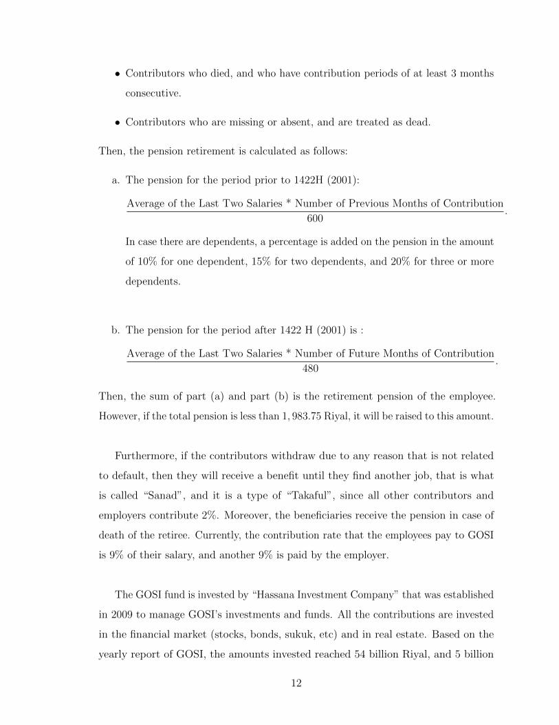
• Contributors who died, and who have contribution periods of at least 3 months

consecutive.

• Contributors who are missing or absent, and are treated as dead.

Then, the pension retirement is calculated as follows:

a. The pension for the period prior to 1422H (2001):

Average of the Last Two Salaries * Number of Previous Months of Contribution

600.

In case there are dependents, a percentage is added on the pension in the amount

of 10% for one dependent, 15% for two dependents, and 20% for three or more

dependents.

b. The pension for the period after 1422 H (2001) is :

Average of the Last Two Salaries * Number of Future Months of Contribution

480.

Then, the sum of part (a) and part (b) is the retirement pension of the employee.

However, if the total pension is less than 1, 983.75 Riyal, it will be raised to this amount.

Furthermore, if the contributors withdraw due to any reason that is not related

to default, then they will receive a benefit until they find another job, that is what

is called “Sanad”, and it is a type of “Takaful”, since all other contributors and

employers contribute 2%. Moreover, the beneficiaries receive the pension in case of

death of the retiree. Currently, the contribution rate that the employees pay to GOSI

is 9% of their salary, and another 9% is paid by the employer.

The GOSI fund is invested by “Hassana Investment Company” that was established

in 2009 to manage GOSI’s investments and funds. All the contributions are invested

in the financial market (stocks, bonds, sukuk, etc) and in real estate. Based on the

yearly report of GOSI, the amounts invested reached 54 billion Riyal, and 5 billion

12

Riyal for real estate.

Some Disadvantages of the Pension Plan in Saudi Arabia.

1- The age of retirement in the public system is 60, and it has never been modified to

keep up with the current changes in the ageing of the populations.

2- Lack of financial sustainability.

3- Very generous system, i.e, the maximum benefit is 100%.

4- Encourages early retirement since 60 is the latest age for retirement.

5- Lack of information about the investment strategy that is used with the plan assets.

1.6.2 Pension Plan In Canada

In the 1950s and 1960s, Canada adopted its current system of retirement income

provision, and it has attracted widespread attention because of its design. It consists

of three separate pillars which are intended to enable retirees to maintain a reasonable

standard of living when they retire. These pillars are:

1. Old Age Security payments..

2. Canada Pension Plan, or the Quebec Pension Plan in Quebec.

3. Private retirement savings including registered pension plans (RPPs), and

registered retirement savings plans (RRSPs) or other personal savings.

In what follows, we give a description of each pillar, and their eligibility rules.

Then, we review how the pension funds are invested under this design.

Old Age Security Pension Plan

In 1951, the federal government introduced the Old Age Security (OAS) to provide

a universal pension plan to all Canadians. Point of the fact, it is the cornerstone of

Canada’s retirement income system. It includes a basic pension, which goes to almost

all citizens who are 65 or older, and who have lived in Canada for more than ten years.

13

As such OAS is Canada’s largest public pension program.

In addition, if the retiree has little or no income other than the OAS pension at

retirement, then he/she may be eligible for the Guaranteed Income Supplement (GIS).

Allowance gives an additional monthly benefit to Canadians who are between 60 and

64, and who have a spouse or common-law partner who is receiving the GIS. If they

are widows or widowers, then there is another additional benefit per month.

Canada Pension Plan

In 1965, the federal government reformed the public pension system, and they

introduced the Canada Pension Plan (CPP), which was implemented as a complementary

measure to OAS. CPP is offered throughout Canada, except in Quebec that has its

own program called the Quebec Pension Plan (QPP) for workers in Quebec. The

Canada Pension Plan pays a monthly retirement pension to employees who have

contributed to the CPP. Furthermore, it provides benefits to the participants and to

their children if they become severely disabled or die during their working years. A

lump-sum death benefit is available to the participants estate when he/she dies.

The contribution amount depends on the participants earnings. Also, the amount

of CPP benefits depends on several factors, for instance, how long a participant

contributed to the plan, how much he/she contributed, and finally, the age at which

they choose to begin receiving their CPP retirement pension which usually is between

60 and 70.

Private Retirement Savings

It consists of employment pension plans and individual retirement savings. To

encourage savings for retirement, the government has created several plans that offer

tax benefits to Canadians. These plans let people avoid or delay some of the tax they

14

would pay otherwise.

For instance, Registered Retirement Savings Plans (RRSPs, tax-deferred accounts),

Tax-Free Savings Account (TFSA), Non-registered Savings and Investments, and Basic

Savings Accounts. Interested readers can refer to the “Financial Consumer Agency of

Canada” web site (http://www.fcac-acfc.gc.ca/eng/Pages/home-accueil.asp).

Figure 1.3: Summary of the Canada Pension Plan Design

CPP funds are invested by the Canada Pension Plan Investment Board (CPPIB)

that emerged out of the realization in the 1990s, that the CPP fund was unsustainable.

Primarily, this was because the Canada Pension Plan benefit payments were exceeding

contributions and changing demographics were leading to fewer workers supporting a

growing number of retirees.

15

Figure 1.4: CPP Returns on Investment Over the Last Five Years

The CPPIB invests the funds of the CPP to help ensure its long-term sustainability,

and it has offices in different cities around the world to help in managing its invesments

internationally. Moreover, CPPIB invests in different ranges of asset classes, internal

and external investments, such as real estate, public and private equities, and

infrastructure. Furthermore, the current asset mix is as follows, 30.9% is in Public

Equities, 18.6% in Private Equities, 34.0% in Fixed Income, and 16.5% in real estate.

The CPP fund ended its third quarter of fiscal year 2015 on December 31, 2014,

with net assets of 238.8 billion dollars, and it is compared to 234.4 billion dollars at the

end of the previous quarter. The investment return was 3.3% for the quarter, although

CPPIB declared that the contribution rate reached 9.9%. Also, based on the CPPIB

report “The CPP Fund is expected to grow significantly between now and 2022, and

Canada’s Chief Actuary predicts that the CPP fund will grow to approximately 340

billion dollar by 2022”.

16

Investment Strategy of CPP

Based on the CPPIB report, the CPPIB investment strategy is comprised of three

key elements; the CPP Reference Portfolio, Value-Adding Active Management and

Total Portfolio Approach. The CPP reference Portfolio is the foundation of the

investment strategy, with low cost and low complexity portfolio of the public market

investments that can achieve the needed return for long-term, under this strategy.

Value-Adding Active Management is the range of public and private market investment

strategies that is employed to add value over the CPP reference portfolio returns.

Then, Total Portfolio Approach is a principal element of the overall investment strategy.

It determines the true underlying risk and return characteristics of each investment.

This allows to manage the overall portfolio with more insight and precision. CPPIB

now is investing 55% of the fund in global equities, 15% in Canadian equity, and 30%

in Canadian Government Bonds.

Figure 1.5: External Investment of CPPIB in 2015

Some Challenges Both Countries Face

1. Increased number of retirees compared to the number of employees.

2. Increased life expectancy, and this puts more pressure on pension plans.

17

3. Low long-term interest rates leads to a decline in pension funds.

4. In Canadian designs, Pillar 2 (CPP/QPP) provides lower benefits than in most

other developed countries.

5. In Pillar 3, “People are not saving enough for retirement and if we let this

go unchecked we are going to face a huge economic crisis.” Kathleen Wynne,

Premier of Ontario, November 12, 2013.

Figure 1.6: Investments (in Billions) by CPPIB in Canada

18

Chapter 2

Risk Measurement

For centuries, insurers and reinsurers have been selling risk coverages. Over time,

they have been joined in this activity by banks and financial institutions. So it is

not surprising that both groups face similar challenges; collecting and managing risks

by looking for markets where these may be hedged or unbundled. However, when a

market hedging of these risks does not exist, then a risk measurement is needed to

allocate and evaluate performance. In this chapter we go over some important results

in risk measurement, as well as some risk measures that are used most often in current

research in actuarial science and finance.

2.1 Coherent Risk Measures

Many literature reviews defined the risk to be the variability in the future value of the

position due to uncertainty. Or it might be the change in the position between two

dates, and then whether those values are acceptable or unacceptable values.

Definition 2.1.1. Artzneret al. in [2] defines a measure of risk, say ρ, as a mapping

from the set of all risks X into a real number R. Mathematically,

ρ : X → R.

In other words, it is to determine a number ρ(X) that quantifies the risk and can

19

serve as a capital requirement. Further, if the value that is assigned by the measure

is positive, then it is interpreted as the minimum extra cash the agent has to add

to the risky position and to invest it to be acceptable. However, if it is negative, an

equivalent cash amount can be withdrawn from the position without affecting its

acceptability.

The functional form and fundamental properties of risk measures have been

extensively studied in the actuarial literature since 1970. Here we list the most

important properties commonly imposed on risk measures;

• Adding or (subtracting) an initial amount say α to the initial position and

investing it, this will lead to a decrease or (an increase) in the risk measure by

α. Mathematically, if ρ is a measure of the risk X, and α is a real number, then

ρ(X + α) = ρ(X) + α.

This property is called “translation invariance”.

• The risk measure for two combined risks will not be greater than that of the

risks measured separately. Mathematically, for all X1 and X2,

ρ(X1 +X2) ≤ ρ(X1) + ρ(X2).

This property is called “sub-additivity”, and it reflects the fact that there should

be some diversification benefit from combining risks.

• Positive homogeneity: for a constant λ ≥ 0, and a riskX,

ρ(λX) = λρ(X).

• Monotonicity: for two risks X and Y such that X ≤ Y , then we have ρ(Y ) ≤

ρ(X).

It is clear that any risk measure should satisfy this property.

20

Sometimes risks increase in a non-linear way, and this leads to suggest the convexity

property which is as following;

ρ(λX1 + (1− λ)X2) ≤ λρ(X1) + (1− λ)ρ(X2).

This property means that the diversification does not increase the risk.

If the measure satisfies all the above conditions, then it is called a convex coherent

risk measure, and if satisfies only the convexity property, then it is called a convex

risk measure; for more details on convex risk measures see Follmer and Schied in [26].

In actuarial science, the first use of risk measures was in the development of

premium principles to determine an appropriate premium to charge for an insurance.

Since then, numerous risk measures have been used to determine not only the premium,

but also the economic capital, that is, how much capital should an insurer hold to

cover future liabilities. These risk measures are ranged from the most elementary to

the most elaborate. In the following section, we illustrate some examples of the most

commonly used risk measures in actuarial science and finance.

2.2 Value at Risk (VaR)

The Value at Risk measure was actually in use by actuaries before it was reinvented for

investment banking, and it is known as the quantile risk measure or quantile premium

principle. In the last decade, VaR has become the established measure of risk exposure

in financial service firms and has even begun to find acceptance in non-financial service

firms. VaR also has roots in portfolio theory and a crude VaR measure was published

in 1945; interested readers in the history of VaR can refer to Jorion in [44].

In fact, VaR was introduced to answer the following question; how much can we

expect to lose in one day, week, year, with a given probability.

21

Definition 2.2.1. The formal definition of VaR measure is as follows;

VaRq(X) = πq, such that P (X ≤ πq) = q.

This definition applies in the continuous case, however, for discrete and mixed

distributed risks X, it is defined as follows;

VaRq(X) = πq = min{πq : P (X ≤ πq) ≥ q},

where 0 ≤ q ≤ 1 is the confidence level. Typical values of q range between 0.95 and

0.99. In general, to obtain VaR, the underlying distribution should be known in

advance.

As a matter of fact, VaR fails to be a coherent risk measure due to its lack of

sub-additivity only, however, if risks follow a normal distribution and independent

then VaR is sub-additive. Another drawback of the value-at-risk measurement is

its inability to recognize an undue concentration of risks. In addition, it has the

property that the VaR of a sum may be higher than the sum of the individual VaRs.

In such a case, diversification will lead to more risk being reported. Note that VaR

is law invariant in a very strong sense; the distributions of X and Y do not need to

be identical in order to imply VaRq(X) = VaRq(Y ). A certain local identity of the

distributions suffices for this implication. In particular, random variables X with light

tail probabilities and Y with heavy tail probabilities may have the same VaR. This

point is also one main criticism against VaR as a risk measure.

2.3 Conditional Value at Risk (CVaR)

Because of the above disadvantages of VaR as a risk measure, and also, the fact that

the VaR does not give any information about the severity of losses beyond the VaR

level, some alternative risk measures have been proposed. For instance, CVaR is a

superior alternative to VaR. It is also known as “Tail Value at Risk”, “Expected

22

Shortfall”, and “Tail Conditional Expectation”, see Artzneret al. in [2], and Tasche

[57]. Although, CVaR is still not used as a standard measure in the finance industry,

CVaR is used more commonly in the insurance industry, and it has been used in credit

risk evaluations; for more details see Embrechtset al. in [25].

Definition 2.3.1. The CVaR measure is defined as below;

TV aRq(X) = CV aRq(X) = E[X|X > VaRq(X)]

However, in general, CVaR is calculated as the weighted average of VaR and losses

exceeding VaR.

Pflug in [52] proved that CVaR is a coherent risk measure with the following properties;

transition-equivalent, positively homogeneous, convex, monotonic w.r.t. stochastic

dominance of order 1, and monotonic w.r.t. stochastic of order 2. Also, CVaR is more

robust with respect to sampling error than VaR.

Furthermore, CVaR can be optimized and constrained with convex and linear programming

methods, but VaR is difficult to optimize. Moreover, CVaR may have a relatively

poor out-of-sample performance compared with VaR if tails are not modeled right.

Hence, mixed CVaR can be a good alternative that gives different weights for different

parts of the distribution; for more details see Uryasev in [55].

Additional risk measures can be used to measure risk. For instance, Markowitz in

[48] and [49] was the first one who recognized the relationship between risk and reward

and introduced the standard deviation as a measure of risk. However, he was also the

first to suggest the semi-standard deviation as an alternative to deal with the standard

deviation’s symmetric nature. The coefficient of variation is a better measure of risk

than the standard deviation and variance. However, it is not a coherent risk measure.

Pension schemes are faced with a number of different types of risk, and there is

strong demand to measure such risks using a good risk measure. In the following

chapter, some risks of pension plans are measured using the above measures.

23

Chapter 3

Model Structure and Assumptions

In this chapter, we describe the model structure of the hybrid plan that we use in this

work. Then, we discuss the modifications that we apply to this plan, as well as, the

notations used.

3.1 Risk Sharing in a Hybrid Pension Plan

Khorasanee in [45] introduced a model for pension plans that allows to share risk

between employees and employers. The structure of this plan follows the DB plan

that was proposed by Dufresne in [20]. Under Dufresne’s plan, the surpluses and

the deficits are amortized by adjusting the contribution income. So, the employers

face all the risks. However, in Khorasanee’s hybrid plan, it is assumed that surpluses

and deficits are not only amortized by adjusting the contribution income, but also by

adjusting the benefit outgo. So, the contribution risk is faced by the sponsor and the

benefit risk is faced by the employee.

The subdivision of risks can be chosen arbitrarily by setting the amortization parameters

in the benefit and contribution to whatever values the plan sponsor deems appropriate.

Moreover, Khorasanee pointed out that the plan with lower aggregate risk, that is the

sum of contribution and benefit risks, is more efficient. The first two moments of the

24

fund and the benefit under this plan are derived, both when the time is finite and

infinite. It is found that the expected benefit at a finite time differs from the target

benefit by some fraction of the difference between the initial value of the fund and the

liability.

In this project, we mainly focus on Khorasanee’s hybrid plan, to which we apply

the following modifications:

• The salary scale is constant, and equal to 1.

• The return on investment is modeled as a time series.

• The valuation rate of interest follows different scenarios.

• Contribution and benefit risks are measured using the value at risk (VaR), and

the coefficient of variation (CV).

3.2 Modeling a Hybrid Plan

In this section, we introduce the model assumptions, notation, and the mathematical

model of a target benefit plan.

3.2.1 Assumptions

In the mathematical discussion, the following model assumptions are made:

1. All the actuarial assumptions are realized exactly, except for investment returns.

2. The population is stationary from the start.

3. There is no inflation on salaries, and no promotional salary scale.

4. The returns on investment are studied under two time series models;

• An autoregressive moving average model, ARMA(1, 1).

• A generalized autoregressive conditional heteroskedasticity

model,GARCH(1, 1).

5. The valuation rate of interest is assumed to be fixed; and in general it is not

necessarily equal to the expected rate of return, as is common in the literature.

25

6. The target benefit is considered to be constant, and equal to 23

of the final salary

which is equal to 1.

7. We consider only the case of active members.

3.2.2 Notation

The variables used in the model are defined as follows:

• Bt is the random benefit at time t.

• Ct is the random contribution rate at time t.

• Ft is the random fund level at time t.

• F0 is the initial value of the fund, and it is assumed to be known.

• it is the random investment return between time t− 1 and time t.

• i = E(it) is the expected rate of return it, assumed constant here.

• Var(it) = σ2i , also assumed constant in time t.

• iv is the known valuation interest rate.

• ALt is the random actuarial liability at time t.

• NCt is the random normal cost rate at time t.

• TNCt is the random terminal normal cost at time t.

• TB is the constant target benefit.

• λ is the spread parameter for the plan. It is equal to 1am

, where m is the

number of years that the unfunded liability is spread into (spread period) for

amortization.

• λc is the spread parameter for the contributions. It is equal to pλ, where

0 < p < 1.

• λb is the spread parameter for the benefits. It is equal to (1− p)λ.

The spread method of amortization is used here, since our goal is to complete

the amortization over a specific number of years m, and 1am

is calculated at rate iv.

Normally, it is assumed that 1 ≤ m <∞, this implies that dv < λ ≤ 1, although it is

possible to consider values of λ out of this range. Also, note that λc + λb = λ in this

study.

26

Moreover, the model is studied under a discrete time scale. Cairns in [15] considered

Dufresne’s model when the time is continuous.

The equations that explain the plan funding, contribution, and benefit are given

as:

Ft+1 = (1 + it+1)(Ft + Ct −Bt), t = 0, 1, .... (3.1)

Ct = NCt + λc(ALt − Ft), t = 0, 1, ..... (3.2)

Bt = TB − λb(ALt − Ft), t = 0, 1, .... (3.3)

Equation (3.1) can be re-expressed as follows, after substituting Ct and Bt from (3.2)

and (3.3);

Ft+1 = (1 + it+1)[(1− λ)Ft + λALt +NCt − TB

]= (1 + it+1)

[(1− λ)Ft +Rt

],

where Rt = λALt +NCt− TB. From the last equation, we can obtain recursively the

following formula for the fund. For t = 1, 2, 3, .....;

Ft = (1− λ)t Πtj=1(1 + ij)F0 +

t−1∑s=0

(1− λ)t−s−1Rs

Πtj=1(1 + ij)

Πsj=0(1 + ij)

,

by setting Πtj=1(1 + ij) = e∆t , and

Πtj=1(1+ij)

Πsj=0(1+ij)= e∆t−∆s , with i0 = 0, we get the final

formula;

Ft = (1− λ)te∆tF0 +t−1∑s=0

(1− λ)t−s−1Rse∆t−∆s . (3.4)

It is clear from equation (3.2) that the contribution rate at time t is the sum of

the normal cost NCt and the adjustment λc(ALt − Ft). Similarly, from equation

(3.3) the benefit at time t is expressed as the difference between the target benefit

TB and the adjustment λb(ALt − Ft). Also, the difference between the expected

liability (ALt) and the actual fund (Ft) is called the unfunded liability; if the

difference is positive, in other words, ALt is greater than Ft, then we have a deficit in

the fund, and the plan contributions should be re-evaluated. However, if the difference

27

is negative, ALt is less than Ft, then we have a surplus in the fund; in this case

the employers might use the excess to cover for future deficits, or, as assumed by

the above equations, use it to decrease contributions Ct or augment benefits Bt, or both.

The terms ALt and NCt are obtained at every evaluation time, using one of the

actuarial cost methods explained in Chapter 1.

Starting from (3.2), (3.3), and (3.4), the first two moments of the fund, the

contribution, and the benefit are derived under the above assumptions, and then the

optimal spread parameter is obtained in Chapter 5 when the time is both finite and

infinite.

28

Chapter 4

Models for the Return on

Investment

Modeling and analyzing financial time series is a complex scientific problem. This

is not only due to the variability of the series in use or to the size of the data that

is available, but also because of the stylized facts that exist in most financial data.

Stylized facts were illustrated by Mandelbrot in [50], and some are mentioned in

Section 3.3. Moreover, financial theory and empirical time series both contain an

element of uncertainty.

The objective of this chapter is to provide some knowledge of financial time series;

in particular asset returns, and introduce some time series models that are useful in

Finance. We begin with a brief introduction of the rate of return. Then, follows a

literature review of various stochastic models that have been used for rates of return

for pension plans. We review some of the most useful time series models used widely

in Finance. Finally, we fit two of these models to the rate of return in a pension plan.

29

4.1 Rate of Return it

Most studies in Finance and Actuarial science model the returns on assets instead

of the actual prices. This is because the rate of return is a complete and scale-free

summary of an investment position, and the statistical properties of this quantity are

more attractive and easier to handle than the price series. However, the continuous

compound return or log-return has some advantage over the actual return; for example,

the continuously compounded multi-period log-return is simply the sum of continuously

compounded one-period log-returns, and the statistical properties of log returns are

more tractable.

In Actuarial Science, in particular in the areas of Life Insurance and Pensions,

authors consider the rate of return as independent and identically distributed (iid)

random variables or as stochastic processes. For instance, Dufresne in [19]-[21],

Haberman in [33], [36], Haberman and Vigna in [41], Haberman and Sung in [37],

Zimbidis and Haberman in [62], Khorasanee in [45] all discuss the case of independent

and identically distributed rates of return. However, time series models have also

been used to model the return. For example, the first order of autoregressive model

AR(1) was applied by Haberman in [32], [34], and [35], Haberman and Gerrad in [39],

Cairns in [14], and Cairns and Parker in [16]. The AR(2) model is also considered

by Haberman in [35]. Haberman and Wong in [38] studied the returns as moving

averages MA(1) and MA(2) models.

4.2 Autoregressive Moving Average (ARMA) Model

ARMA models are used widely to describe data. This may due to the need of

higher-order models with many parameters to explain the dynamic structure of data.

Basically, ARMA models are linear processes which combine autoregressive and

moving average terms into a single form. Although the chance of using an ARMA

30

model in Finance is low, the concept of ARMA models is highly relevant in volatility

modeling, as we see in the next section.

Definition 4.2.1. The log of return series {δt ; t ∈ Z} is an ARMA(p, q) process if

{δt} is stationary and if for every t,

δt − φ1δt−1 − ....− φpδt−p = µ(1− φ1 − ...− φp) + Zt + θ1Zt−1 + .....+ θqZt−q,

where δt = ln(1+it) is the force of interest in the interval (t−1, t), {Zt} ∼White Noise

(0, σ2z), µ is the long mean of the process, and the polynomials (1− φ1B − .....− φpBp)

and (1 + θ1B + .....+ θqBq) have no common factors, where B is back-shift operator

such as BXt = Xt−1.

In this section, we study the simplest ARMA(1, 1) model, and we assume that

{Zt} are independent and identically distributed normals with zero mean and unit

variance. Hence;

δt − φδt−1 = µ(1− φ) + Zt + θZt−1.

where φ + θ 6= 0. The conditions for stationary and the existence of an invertible

solution of the model are that |φ| < 1 and |θ| < 1, respectively.

Figure 4.1: Simulated Data from ARMA(1, 1) with φ = .9 and θ = .1

31

Figure 4.2: Simulated Data from ARMA(1, 1) with φ = −.5 and θ = .5

4.2.1 Marginal Moments under ARMA(1, 1)

Here, the expected value, the variance, and the auto-covariance functions of δt are

derived first. Similarly, the same quantities are obtained for the function ∆t, since it

is needed in the following chapter, and is defined as;

∆t =t∑

j=1

δj.

Hence,

E(δt) = µ ; for all t ∈ Z

To find the variance of the process, the Yule-Walker method is one possible approach

that can be used to derive the auto-covariance of the process,

γδ(m) = γδ(t+m, t) = Cov(δt+m, δt) = E[(δt+m − µ)(δt − µ)];

and it is generally defined for ARMA(p, q) as;

γδ(m)−φ1γδ(m−1)−φ2γδ(m−2)−........−φγδ(m−p) = σ2z

∞∑j=0

ψjθ{j+m} ; m = 0, 1, ..., p

where ψ0 = 1, ψj =∑p

k=1 φkψj−k + θj for j = 0, 1, ...., and θj = 0 for j > q. The

above formula can be used then to find γδ(m) for different values of m. In case of

32

ARMA(1, 1) model, Yule-Walker is adapted as;

γδ(m)− φγδ(m− 1) = σ2z

∞∑j=0

ψjθ{j+m} ; m = 0, 1

then, a system of two equations is generated, and it is used to find the variance of the

process, which is derived as;

Var(δt) = γδ(0) =1 + 2φθ + θ2

1− φ2. (4.1)

which is constant in time under this model.

Then we get;

γδ(1) = θ + φγδ(0).

The auto-covariance function of the process at lag h is then defined recursively as;

γδ(h) = φh−1γδ(1), for any h ≥ 2.

For ∆t, the expectation and the variance are defined as follow;

E(∆t) = tµ.

E(∆t −∆s) = (t− s)µ.

Var(∆t) =[θ + φγδ(0)

][tφ+ 2

t∑i=1

t∑j=i+1

φj−i−1]. (4.2)

For s = 0, 1, 2, ...., t− 1, and assuming that s > v;

Var(∆t −∆s) = Var(t∑

i=s+1

δi) = Cov(t∑

i=s+1

δi,t∑

j=s+1

δj) =t∑

i=s+1

t∑j=s+1

γδ(i, j)

= (θ + φγδ(0))[(t− s) (φ+

2

1− φ)− 2

(1− φt−s)(1− φ)2

].

(4.3)

Var(∆t −∆s + ∆t −∆v) = Var(∆v −∆s + 2(∆t −∆v))

= Var(∆v −∆s) + 4Var(∆t −∆v) + 4Cov(∆t −∆s,∆t −∆v)

=v∑

i=s+1

v∑j=s+1

γ(i, j) + 4t∑

i=v+1

t∑j=s+1

γ(i, j).

(4.4)

Before concluding this section, we summarize some of the most common properties

of ARMA(1, 1) processes:

33

• The stationarity condition of an ARMA(1, 1) model is the same as that of

an AR(1) model, and the plot of the autocorrelation function ACF of an

ARMA(1, 1) shows a pattern similar to that of an AR(1) model except that

the pattern starts at lag 2.

• ARMA models are applied to model the conditional expectation of a process

given the past information, however, in an ARMA model the conditional and

marginal variance is constant.

4.3 Generalized Autoregressive Conditional

Heteroskedasticity (GARCH)

We mentioned in the introduction of this chapter that financial series have stylized

features or stylized facts, described by Mandelbrot in [50]. We review here some of

the most commonly used in the financial literature.

Figure 4.3: Saudi Arabia TASI Index for 2011-2015 (from TASI website)

34

Figure 4.4: Canada S&P/TSX Toronto Stock Market Index for 2011-2015 (from

S&P/TSX Toronto Stock Market website)

Figure 4.5: CAC 40 Index for the Period from March 1, 1990 to October 15, 2008

(from Francq and Zakoian in [27])

Properties of financial time series:

1. Generally financial time series are not stationary as it is clear from Figures 4.3,

4.4, and 4.5.

35

Figure 4.6: Saudi Arabia TASI Index for 2011-2015

Figure 4.7: Canada S&P/TSX Toronto Stock Market Index for 2011-2015 (from

S&P/TSX Toronto Stock Market website)

2. Some series display small autocorrelations, making them close to a white noise

as illustrated in Figures 4.8, 4.9, and 4.10.

36

Figure 4.8: Sample Autocorrelations of Returns of the TASI (Feb. 23, 2013 to Feb.

23, 2016)

3. The square and absolute values of the processes show strong autocorrelations,

see Figure 4.11.

Figure 4.9: Sample Autocorrelations of Returns of the CAC 40 from January 2, 2008

to October 15, 2008 (from Francq and Zakoian in [27])

37

Figure 4.10: Sample Autocorrelations of Returns of Canada S&P/TSX Toronto Stock

Market Index from Feb. 23, 2011 to Feb. 23, 2016

Figure 4.11: Sample Autocorrelations of Squared Returns of the CAC 40 from January

2, 2008 to October 15, 2008 (from Francq and Zakoian in [27])

4. Volatility clustering, which means large changes are followed by large changes,

and small changes follow small changes. This is clear in the square and the

absolute values of the series.

5. Financial series can have fat tails, so then they are called leptokurtic.

6. Calendar effects, holidays, days of the week, and other seasonal patterns, may

have significant effects on the series.

38

For further explanations see Mandelbrot in [50] or Francq and Zakoian in [27].

As we see from these properties it is difficult to model financial time series, so

there is a need for a stationary model that captures the main stylized facts of the

series. Hence, the ARMA(1, 1) is not appropriate to fit the data because it assumes a

constant variance, meaning that the conditional variance is time-invariant and contains

no past information. So, conditional heteroscedasticity is preferred, together with the

stationarity property.

Conditional heteroscedastic models were introduced to the Econometrics literature

to account for the very specific nature of financial series, and they have been

used extensively in research. In this section, we mainly focus on the generalized

autoregressive conditional heteroscedastic GARCH model.

Engle in [23] introduced the autoregressive conditional heteroskedastic ARCH

model to allow the conditional variance to vary over time, as a function of the past

errors. Similarly to the extension of AR models to ARMA models; an extension of

ARCH models is proposed by Bollerslev in [6] to allow for a more flexible lag structure,

and permit a wider range of behavior, in particular, more persistent volatility.

Definition 4.3.1. The process {δt ; t ∈ Z} is called GARCH(p, q) if

δt = Υ + εt,

where Υ is the long mean of the process under GARCH.

εt = σtZt,

σ2t = α0 +

p∑i=1

αiε2t−i +

q∑j=1

βjσ2t−j,

and Zt as well as σ2t are real processes such that:

• The volatility process σ2t is measurable with respect to the history σ-field,

denoted Ft−1 = σ(εs; s < t). Hence, the volatility is a deterministic function of

the past εt.

39

• Zt ∼ iid random variables, and Zt is independent of Ft−1.

• α0 > 0, αi > 0, and βj > 0 to guarantee that the conditional variance is

non-negative.

• For j = 1, ...., q, if βj = 0, the process is called ARCH(p) process.

For simplification, here the standard GARCH(1, 1) is considered, where Zt follows a

normal distribution with zero mean and unit variance. However, substantial research

work has been devoted to the model when the error Zt follows other distributions,

such as the t-distribution, Z-distribution, gamma distribution, generalized Pareto

distribution; see Bai, Russel, and Tiao in [4], Bollerslev in [7], and Lanne and Pentti

in [47]. So, the conditional variance of the GARCH(1, 1) is given as;

σ2t = α0 + α1ε

2t−1 + β1σ

2t−1, (4.5)

where α1 + β1 < 1 to ensure stationarity. Moreover, α1 + β1 is the persistence

measurement.

Figure 4.12: Simulated data from GARCH(1, 1) with α0 = 1, α1 = .4, and β1 = .5,

As pointed out in the literature, the squared process {ε2t} can be represented as

an ARMA(1, 1) model by adding ε2t to equation (4.5) to get;

σ2t + ε2

t − ε2t = α0 + α1ε

2t−1 + β1σ

2t−1,

40

ε2t − (α1 + β1)ε2

t−1 = α0 + ν2t − β1ν

2t−1, (4.6)

where ν2t = ε2

t − σ2t = ε2

t − E(ε2t |Ft−1). Moreover, ν2

t is a white noise with mean zero

and variance σ2ν2 that is given as;

Var(ν2t ) = E(ε2

t )−α2

0

(1− β1)2− α2

1

∞∑i=0

∞∑j=0

βi1βj1E(ε2

t−(i+1)ε2t−(j+1))

+2α0α1

1− β1

∞∑j=0

βj1E(ε2t−(j+1)).

Furthermore, GARCH(1, 1) processes can be represented as ARCH(∞), which

allows to write σ2t as function of the infinite sum of past ε2

t values in the form;

σ2t = w0 +

∞∑i=1

wiε2t−i,

where w0 = α0

1−β1 , and wi = α1βi−11 .

4.3.1 Conditional Moments of the GARCH(1, 1) Model

Here, the conditional moments such as the first and the second moments of εt, δt, and

∆t are listed;

E(εt|Ft−1) = 0.

σ2t = Var(εt|Ft−1) = E(ε2

t |Ft−1).

Cov(εt, εt+h|Ft−1) = 0.

then by using the above moments, the moments of our functions are derived as below;

E(δt|Ft−1) = Υ.

Var(δt|Ft−1) = Var(ε2t |Ft−1) = σ2

t .

E(∆t|Ft−1) = tΥ.

Var(∆t|Ft−1) =t∑i=1

σ2i .

41

4.3.2 Marginal Moments of the GARCH(1, 1) Model

Bollerslev in [6] states a theorem that helps find the even moments, and he provides

sufficient conditions for the existence of the even order 2m moments, for m = 1, 2....

Note that, for the odd moments; that is of order 2m− 1, are all equal to zero, due to

symmetry.

Theorem 4.3.1. For the GARCH(1, 1) process given above a necessary and sufficient

condition for existence of the 2mth moment is

µ(α1, β1,m) =m∑j=0

(m

j

)ajα

j1β

m−j1 < 1,

where a0 = 1, aj = Πji=1(2j − 1).

Then, the 2m-th moment can be expressed by the recursive formula;

E(ε2mt ) =

am

[∑m−1n=0 a

−1n E(ε2n

t )αm−n0

(m

m−n

)µ(α1, β1, n)

]1− µ(α1, β − 1,m)

.

Hence, the first four moments of εt are given as;

E(εt) = E(σt)E(Zt) = 0.

E(ε2t ) =

α0

1− α1 − β1

.

E(ε3t ) = 0.

E(ε4t ) = 3

α20(1 + α1 + β1)

(1− α1 − β1)(1− β21 − 2α1β1 − 3α2

1).

Then,

Var(εt) = σ2ε = γε(0) =

α0

1− α1 − β1

.

Cov(εt, εt−h) = 0.

Skewness(εt) = 0.

Kurtosis(εt) = 3(1 + α1 + β1)(1− α1 − β1)

(1− β21 − 2α1β1 − 3α2

1).

42

The marginal moments of our target functions;

E(∆t) = tΥ.

Var(∆t) = tα0

1− α1 − β1

.

For s = 0, 1, ....t− 1, and v > s,

E(∆t −∆s) = (t− s)Υ.

Var(∆t −∆s) = (t− s) α0

1− α1 − β1

.

Var(2∆t −∆s −∆v) = (v − s) α0

1− α1 − β1

+ 4(t− v)α0

1− α1 − β1

.

It is clear that the auto-covariance of the process εt is equal to zero which means

that the random variables are uncorrelated although they are dependent, thus the

process is weak white noise. As a consequence the square of the process is also

considered in the literature, since the auto-covariance is not equal to zero;

Cov(ε2t , ε

2t+h) = γε2(h) = (α1 + β1)|h|γε2(0),

where h ∈ Z, and γε2(0) = Var(ε2t ).

Although the marginal distribution of εt is not known explicitly, we can have an

idea of the shape of the distribution from the marginal moments of the GARCH

model. Hence, from the above moment formulas we can highlight some properties of

the distribution:

• The skewness of the process is zero which means that the distribution is

symmetric.

• The kurtosis of the process is greater than 3, and that means that the process is

leptokurtic.

• When 0 < α1 < .06 and 0 < β1 < .9, the kurtosis is approximately equal to 3.

43

Finally, it is interesting to mention the following additional properties of GARCH

models that are considered in the Economics literature, to conclude this section:

1. The forecasting value of the conditional variance after multiple steps, say L, is

obtained as;

σ2t+L = σ2

εt + (α1 + β1)L(σ2t − σ2

ε), (4.7)

where σ2 is the unconditional variance of εt. Hence, as L→∞, σ2t+L → σ2

ε .

2. From (4.7) we notice that α1+β1 determines how quickly the forecasting variance

approaches the unconditional variance.

3. The initial value of the conditional variance can be set to the sample variance,

to α0, or to the unconditional variance.

4. There are other types of GARCH models that can be found in the literature

such as Integrated GARCH (IGARCH), Fractional IGARCH (FIGARCH),

Exponential GARCH (EGARCH). Some of these are reviewed in the next

section.

4.4 Long-Memory Models

Long-memory processes are known to play an important role in many scientific

disciplines and applied fields such as Physics, Geophysics, Hydrology, Economics,

Finance or Climatology. Furthermore, they have been used in Economics since 1980,

and there is a considerable evidence that this type of process successfully describes

financial data such as forward premiums, inflation rates, and exchange rates. Currently,

it is believed that long memory models are better candidates than other conditional

heteroscedastic models to explain volatility in stock returns and exchange rates; for

more details see Granger, Ding, and Engle in [30], Harvey in [40], Granger and Ding

in [31].

Definition 4.4.1. Given a discrete time series Yt with autocorrelation ρ(j) at lag j

44

and spectral density function fy(λ), the process is long memory process if

limn→∞

n∑j=−n

|ρ(j)|

is non-finite or diverges; or as λ→ 0, fy(λ) diverges.

Long-memory is also called strong memory, hyperbolic memory, long-range dependence

or long-range correlation. Moreover, under this process the sample auto-correlations

decline to zero hyperbolically rather than geometrically. However, if the sample

autocorrelations of the process decay geometrically to zero, then the process is classified

as a short memory process.

In this section, we go over some examples of time series models that exhibit long

memory, and we review the most common features or characteristics of those models.

4.4.1 Autoregressive Fractionally Integrated Moving Average

Model (ARFIMA)

When the data is stationary, and its autocorrelation function exhibits a rapidly decrease

to zero, then ARMA models give a better fit. However, if the data does not exhibit

these properties, then we need to difference the data until it produces new series

that has ARMA characteristics. Thus, we say that the original series follows an

autoregressive integrated moving average model (ARIMA).

In fact, ARMA and ARIMA processes are preferable models in time series, and

this is due to their simplicity and flexibility. The definition of an ARIMA model is

given below.

Definition 4.4.2. If d is a nonnegative integer, then the series {Xt} is an

ARIMA(p, d, q) process if (1−B)dXt is an ARMA(p, q) process. Thus,

φ(B)(1−B)dXt = θ(B)Zt,

45

where {Zt} ∼WN(0, σ2z), φ(B) = 1 − φ1B − .... − φpBp, and θ(B) = 1 + θ1B +

.....+ θqBq. If d = 0, then the model reduces to an ARMA process. In other words,

ARMA is a special case of the ARIMA process. In Econometrics, Xt is also called

an integrated process of order d, or I(d).

Granger and Joyeux in [29], and Hosking in [43] introduced a model that is between

an ARMA and ARIMA, and it allows d to be non-integer; this model is called

autoregressive fractionally integrated moving average ARFIMA. In other words, it

is defined as follows.

Definition 4.4.3. If d ∈ (−12, 1

2), the process {Xt} is ARFIMA if

φ(B)(1−B)dXt = θ(B)Zt,

where (1−B)d is defined as an hypergeometric function;

(1−B)d =∞∑j=0

Γ(j + d)

Γ(j + 1)Γ(d)Bj.

Palma in [53] discusses the ARFIMA process and shows that it is stationary and

invertible, if the roots of φ(B) and θ(B) lie outside the unit circle.

4.4.2 Fractionally Integrated Generalized Autoregressive

Conditional Heteroscedastic (FIGARCH)

Under the GARCH model, we mentioned that α1 + β1 measures the persistence, and

as this sum approaches 1, the greater the persistence of shocks to volatility. So, if

α1 + β1 = 1, then the current shock persists indefinitely in conditioning the future

variance. Hence, Engle and Bollerslev in [24] proposed an extension of GARCH, and

called integrated GARCH (IGARCH).

Definition 4.4.4. The IGARCH model is defined as;

L(B)(1−B)ε2t = α0 + (1− β1B)ν2

t ,

where L(B) = (1− α1B − β1B)(1−B)−1, and α1 + β1 = 1.

46

A key feature of the IGARCH model is that the impact of the past squared shock

is persistent and the pricing of risky securities, including long-term options and future

contracts, may show extreme dependence on the initial conditions. However, the

unconditional variance under this model is infinite. Moreover, the forecasting of future

conditional variance approaches the current conditional variance since α1 + β1 = 1,

see (4.7). Choudhry in [18] tested a real data made of stock returns from different

countries, using IGARCH to check for the persistence of shocks to volatility.

Davidson in [22] mentions that both GARCH and IGARCH have short memory.

In other words, it is shown that GARCH and IGARCH models have a memory

which is much shorter than financial series generally exhibit. Breidt, Crato and de

Lima in [10], Granger, Ding, and Engle in [30], Granger and Ding in [31], and Harvey

in [40] all noticed the presence of long-memory in the autocorrelations of squared and

absolute returns of various financial asset prices. Motivated by these observations, the

fractional IGARCH (FIGARCH) was introduced.

The main feature of this model is that it provides a more flexible class of processes

for the conditional variance that are better capable of explaining and representing

the observed temporal dependencies in financial market volatility. In particular, the

FIGARCH model exhibits a slow hyperbolic rate of decay for the lagged squared or

absolute innovations in the conditional variance function.

Definition 4.4.5. The process {εt} follows a FIGRACH model if

L(B)(1−B)dε2t = α0 + (1− β1B)ν2

t ,

where 0 < d < 1.

The proof of stationarity in the general case of FIGARCH(p, d, q) is not yet

available. Also, the process has an infinite unconditional variance. A good review of

FIGARCH models can be found in Tayefi and Ramanathan in [58].

47

Finally, the interested reader can refer to Beran, Feng, Ghosh, and Kulik in [5] for

more details. Baillic in [3] provides a good survey about long memory processes and

fractional integration in Econometrics.

48

Chapter 5

Risk Measurement under Hybrid

Pension Plan

Hybrid pension plans are subject to different type of risks; some of them were

mentioned in Chapters 1 and 3. For instance, the contribution risk represents

the size of deviations in the normal cost and is related to the stability of the plan.

In the literature the contribution risk is usually measured by the variance of the

contribution rate Var(Ct). Another type of risk is the solvency risk, when the

pension fund can either meet its liabilities or the plan has to be wound up. In other

words, this risk is an indicator of the financial stability of the plan. The variation in

pension funds is measured in this case using the variance Var(Ft). For the employees,

the stability and predictability of the benefit is important for financial planning.

Hence, it is desirable to keep the variations in benefit in an acceptable range, and

the variance Var(Bt) is often used as a measure; this type of risk is called benefit risk.

In this chapter, we study these risks under the proposed hybrid plan. The expected

value and the variance of the fund, the annual contribution rate, and the annual benefit

rate are derived when the rate of return follows an ARMA(1, 1) and GARCH(1, 1)

process for t → ∞ as well as t < ∞. Moreover, all the actuarial valuations of the

plan are done when the valuation interest rate iv is not necesarilly equal the expected

rate of return E(it), taking into account the special case when iv = E(it). Then, the

49

aggregate risk, which is defined as the sum of the contribution risk and the benefit

risk, is obtained under different risk measure and as t goes to infinity. Finally, the

optimal spread parameter λ∗ is considered by minimizing the aggregate risk.

5.1 Moments of the Fund, Contribution, and Benefit

Levels

It is clear from (3.2) and (3.3) that the contribution and the benefit levels depend on

the fund level. Hence, we start with the fund dynamics equation, to obtain the first

two moments under each rate-of-return models.

For t = 0, 1, 2, 3, ...., equation (3.1) can be re-expressed as follows;

Ft+1 = (1 + it+1)[(1− λ)Ft + λALt +NCt − TB

]= (1 + it+1)

[(1− λ)Ft +Rt

].

(5.1)

Since the population is stationary, we can drop t from Rt, ALt, and NCt, and assume

that they reached their stationary constant values.

By taking the expectation on both sides in equation (5.1), we get the following:

E(Ft+1) = qE(Ft) +R(1 + i),

where q = (1 + i)(1− λ).

Then, we obtain recursively the following equation for t = 1, 2, ...;

E(Ft) = qtF0 +R(1 + i)1− qt

1− q. (5.2)

For the variance of the fund, the formula is given as;

Var(Ft) = bt∑

j=1

at−j(E(Fj))2, (5.3)

50

where a = (1− λ)2[(1 + i)2 + σ2i ], and b = σ2

i (1 + i)−2.

These formulas are derived under the assumption that the rates of return are

independent and identically distributed random variables; the case studied by Dufresne

in [20] and Khorasanee in [45]. However, here we are assuming that the rates of return

follow a time series model, hence the independence assumption is not true any more.

5.1.1 Moments of the Fund Level under ARMA(1, 1)

Recall equation (3.4) from Chapter 3;

Ft = (1− λ)te∆t +Rt−1∑s=0

(1− λ)t−s−1e∆t−∆s .

Taking expectation of both sides, we have the following;

E(Ft) = (1− λ)tF0 E(e∆t) +Rt−1∑s=0

(1− λ)t−s−1E(e∆t−∆s). (5.4)

As we see from the above equation; E(e∆t) and E(e∆t−∆s) are needed. It is known

that under an ARMA(1, 1) model the marginal distribution of δt are normal; because

the residual Zt are assumed independent and identically normal distributed. Hence,

eδt has a log-normal distribution with mean and variance given as;

E(eδt) = exp{µ+1

2γδ(0)},

Var(eδt) = (eγδ(0) − 1)(e2µ+γδ(0)),

where γδ(0) is given in equation (4.1).

Then, for ∆t and ∆t −∆s, which are functions of δt, are also normally distributed.

Hence, e∆t and e∆t−∆s follow a log-normal distribution, and their means are obtained

as follow;

E(e∆t) = exp{tµ+

1

2(θ + φγδ(0))

[tφ+ 2

t∑j=1

t∑i=j+1

φi−j−1]}

= ηt1 e−ξ(1−φt),

(5.5)

51

E(e∆t−∆s) = exp{

(t− s)(µ+

1

2(θ + φγδ(0))(φ+

2

1− φ))}

exp{−(θ + φγδ(0))

(1− φ)2(1− φt−s)

}= ηt−s1 eξ(φ

t−s−1),

(5.6)

where η1 = exp{µ+ 1

2(θ + φγδ(0))(φ+ 2

1−φ)}

, and ξ = (θ+φγδ(0))(1−φ)2

.

Then, by substitution of equations (5.5) and (5.6) into equation (5.4), the following

formula for the expectation of the fund is obtained;

E(Ft) = (1− λ)tF0 ηt1 e−ξ(1−φ

t) +Rt−1∑s=0

(1− λ)t−s−1ηt−s1 eξ(φt−s−1). (5.7)

The second moment of the fund is derived by squaring both sides of equation (3.4)

and then rearranging the terms;

E(F 2t ) = (1− λ)2t F 2

0 E(e2∆t) + 2R(1− λ)t F0

t−1∑s=0

(1− λ)t−s−1E(e∆t+∆t−∆s)

+R2

t−1∑v=0

t−1∑s=0

(1− λ)t−s−1 (1− λ)t−v−1 E(e∆t−∆s+∆t−∆v)

= (1− λ)2t F 20 E(e2∆t) +

2 R

(1− λ)F0

t−1∑s=0

(1− λ)2t−sE(e2∆t−∆s)

+R2

(1− λ)2

[ t−1∑s=0

(1− λ)2(t−s)E(e2(∆t−∆s)) + 2t−1∑v=1

v−1∑s=0

(1− λ)2t−s−v

E(e2∆t−∆s−∆v)].

(5.8)

It is clear that the equation (5.8) depends on the terms E(e∆t), E(e∆t−∆s), and

E(e2∆t−∆s−∆v). Hence, we still need to find the last term.

For v > s, we have the following;

E(e∆t−∆s+∆t−∆v) = exp{

(t− s)µ+ (t− r)µ+ (θ + φγδ(0))H(t, v, s)}

= ηt−s1 ηt−v2 e−3ξ e2ξφ(t−s) e2ξφ(t−v) ,(5.9)

52

where

H(t, s, v) =1

2

v∑j=s+1

v∑i=s+1

φ|i−j−1| + 2t∑

j=v+1

t∑i=s+1

φ|i−j−1|

=1

2(t− s)

(φ+

2

1− φ

)+

3

2(t− v)

(φ+

2

1− φ

)+

1

(1− φ)2

(2φt−s + 2φt−v − 3

).

and η2 = exp{µ+ 3

2(θ + φγδ(0))(φ+ 2

1−φ)}

, while η1 and ξ are give as before.

Then, by substitution of equations (5.5), (5.6), and (5.9) into (5.8);

E(F 2t ) = (1− λ)2tF 2

0 η2t1 e−2ξ(1−φt) +

2R F0

(1− λ)

t−1∑s=0

(1− λ)2t−s exp{

(t− s)µ+ tµ+

(θ + φγδ(0))H(t, s, 0)}

+R2

(1− λ)2

t−1∑s=0

(1− λ)2(t−s)η2(t−s)1 e−4ξe4ξφt−s

+2R2

(1− λ)2

t−1∑v=1

v−1∑s=0

(1− λ)2t−s−vηt−s1 ηt−v2 e−3ξe2ξφ(t−s) e2ξφ(t−v) .

(5.10)

The first and the second moments can be simplified as;

E(Ft) = (1− λ)t ηt1e−ξ(1−φt)F0 +R e−ξη1

[1− (1− λ)tηt11− (1− λ)η1

+ Sk

],

where Sk =∑∞

k=1zkφk

k!

1−(1−λ)tηt1φkt

1−(1−λ)η1φk.

E(F 2t ) = (1− λ)2tη2t

1 e−2ξ(1−φt)F 20 +

2 R F0

(1− λ)

2t−s∑s=0

(1− λ)2t−s exp{

(2t− s)µ

+ (θ + φγδ(0))H(t, s, 0)}

+R2e−4ξη21

[1− (1− λ)2tη2t1

1− (1− λ)2η21

+ Sk1

]+

2 R2 e−3ξη1

(1− λ)

{∞∑k2=0

∞∑k3=0

(2ξ)k2+k3φk2

k2!k3!(1− (1− λ) η1φk2)[(1− λ)2η1η2φ

k2+k3(1− (1− λ)2(t−1)ηt−1

1 ηt−12 φ(k2+k3)(t−1)

1− (1− λ)2η1η2φk2+k3

)− (1− λ)(t+1)ηt1η2φ

tk2+k3(1− (1− λ)t−1ηt−1

2 φk3(t−1)

1− (1− λ)η2φk3

)]},

53

where Sk1 =∑∞

k1=1(4ξφ)k1

k1!(

1−(1−λ)2tη2t1 φk1t

1−(1−λ)2η21φk1

).

Hence, simple substitution of equations (5.7) and (5.10) in the variance formula

complete its deviation.

The expectations of the contribution and the benefit levels are given as;

E(Ct) = NC + λc(AL− E(Ft)), (5.11)

E(Bt) = TB − λb(AL− E(Ft)), (5.12)

where E(Ft) is given in equation (5.7), and the spread parameters λc and λb are chosen

for contributions and benefits respectively. We will denoate by λ = λc + λb the total

spread parameters.

The variance of these cash flows is given as;

Var(Ct) = λ2cVar(Ft), (5.13)

Var(Bt) = λ2bVar(Ft), (5.14)

where Var(Ft) is obtained from equations (5.7) and (5.10).

Remark 5.1.1. Ultimate Case (t→∞)

In a stationary population it is interesting to study the behavior of the moments of

the fund, when the time t goes to ∞.

For (1− λ)η1 < 1, E(F∞) is derived as;

E(F∞) = R e−ξη1

[ 1

1− (1− λ)η1

+ S∗k

], (5.15)

where S∗k =∑∞

k=1zkφk

k!1

1−(1−λ)η1φk.

54

Existence E(F 2∞) require that (1− λ)η1 < 1 and (1− λ)2η1η2 < 1, thus;

E(F 2∞) = R2e−4ξη2

1

[ 1

(1− (1− λ)2η21)

+ S∗k1

]+

2R2e−3ξη1

(1− λ){ 1

1− (1− λ)η1

( (1− λ)2η1η2

(1− (1− λ)2η1η2)

)+

∞∑k3=0

Sk2 + Sk3

},

(5.16)

where S∗k1 =∑∞

k1=1(4ξφ)k1

k1!( 1

1−(1−λ)2η21φk1

), Sk2 =∑∞

k2=1(2ξ)k2+k3φk2

(k2)!(k3)!(1−(1−λ)η1φk2 )

(1−λ)2η1η2φk2+k3

1−(1−λ)2η1η2φk2+k3,

and Sk3 =∑∞

k3=1(2ξ)k3

k3!(1−(1−λ)η1φ)( (1−λ)2η1η2φk3

1−(1−λ)2η1η2φk3).

5.1.2 Moments of the Fund Level under GARCH(1, 1)

In order to determine the first and second moments of the fund Ft under the

GARCH(1, 1) model, we need to consider the terms E(e∆t), E(e∆t−∆s), and E(e2∆t−∆s−∆v)

in equations (5.4) and (5.8).

As we mentioned in the previous chapter under GARCH models, when 0 ≤ α1 ≤ .06

and 0 ≤ β1 ≤ .9, then the kurtosis of the model is approximately equal to 3. Also,

the skewness of the model is equal to zero, so we can assume that δt follows normal

distribution. Thus, following the same arguments of the previous section, it can be

shown that

E(e∆t) = exp{tΥ +

1

2tγε(0)

}= κt1,

(5.17)

E(e∆t−∆s) = exp{

(t− s)Υ +(t− s)

2γε(0)

}= κt−s1 ,

(5.18)

E(e2∆t−∆s−∆v) = exp{

(t− s)(Υ +

1

2γε(0)

)+ 3(t− v)

(Υ + γε(0)

)}= κt−s1 κt−v2 ,

(5.19)

where γε(0) = Var(εt) = α0

1−α1−β1 , κ1 = exp{Υ + 12γε(0)}, and κ2 = exp{Υ + 3

2γε(0)}.

55

Then, the first and the second moments of the fund are given as below;

E(Ft) = (1− λ)tκt1 F0 +R

(1− λ)

t−1∑s=0

(1− λ)t−sκt−s1

= (1− λ)tκt1 F0 +R κ1 (1− (1− λ)tκt11− (1− λ)κ1

).

(5.20)

E(F 2t ) = (1− λ)2tF 2

0 κ2t1 +

2 R F0

(1− λ)

t−1∑s=0

(1− λ)2t−sκ2t−s1 +

R2

(1− λ)2

t−1∑s=0

(1− λ)2(t−s)κ2(t−s)1 +

2R2

(1− λ)2

t−1∑v=1

v−1∑s=0

(1− λ)2t−s−vκt−s1 κt−v2

= (1− λ)2tκ2t1 F

20 + 2 R F0(1− λ)tκt+1

1

(1− (1− λ)tκt11− (1− λ)κ1

)+R2κ2

1

(1− (1− λ)2tκ2t1

1− (1− λ)2κ21

)+

2R2 κ1

(1− λ)(1− (1− λ)κ1)[(1− λ)2κ1κ2

1− (1− λ)2(t−1)κt−11 κt−1

2

1− (1− λ)2κ1κ2

− (1− λ)t+1κt1κ2

1− (1− λ)t−1κt−12

1− (1− λ)κ2

].

(5.21)

A simple substitution of equations (5.20) and (5.21) into the variance formula gives

the variance.

Remark 5.1.2. Ultimate Case (t→∞)

As before we consider the behavior of the moments when t goes to ∞ under the

GARCH(1, 1) model.

It is clear that E(F∞) and E(F 2∞) exist only if (1 − λ)κ1 < 1 and (1 − λ)2κ1κ2 < 1

respectively. Thus;

E(F∞) =R κ1

(1− (1− λ)κ1). (5.22)

E(F 2∞) =

R2κ21

(1− (1− λ)2κ12)

+2R2 κ2

1κ2(1− λ)

(1− (1− λ)κ1)(1− (1− λ)2κ1κ2). (5.23)

56

5.1.3 Comments on the Moments of Cash Flows

In general, it is noticeable that when t → ∞, there is a difference between the

first and the second moments of the fund under iid, ARMA(1, 1), and GARCH(1, 1)

models. This difference comes from the exponential terms that are used in modeling δt.

Haberman in [32] and [35] considered an approximation for E(Ft) and E(F 2t ) under

AR(1), AR(2), and MA(1) and studied the errors of approximation; so, following

the same arguments for ARMA(1, 1) we get the following results:

E(F∞) ≈ Re−ξη1

1− (1− λ)η1

,

E(F 2∞) ≈ R2e−4ξη2

1

1− (1− λ)2η21

+2R2e−3ξη2

1η2(1− λ)

(1− (1− λ)η1)(1− (1− λ)2η1η2).

Also, under GARCH model, we choose the following range of the parameters;

0 < α0 ≤ .00001 ; 0 < α1 ≤ .0001 ; 0 < β1 ≤ .1,

1− 1√κ1κ2

< λ ≤ 1,

to avoid any infringement of the conditions (1− λ)κ1 < 1 and (1− λ)2κ1κ2 < 1.

Finally, it is sufficient to consider the following range for λ, max{dv, 1− 1√η1η2} ≤ λ ≤ 1

under ARMA and max{dv, 1− 1√κ1κ2} ≤ λ ≤ 1 under GARCH, to avoid any negative

values for the fund.

Models of it limt→∞ E(Ft) = E(F∞)

iid (1− λ)(1 + i) < 1 ≡ λ > d = ii+1

ARMA(1, 1) (1− λ)η1 < 1 ≡ λ > 1− η−11 ≡ marma <

1δln( η1−1

vη1−1)

GARCH(1, 1) (1− λ)κ1 < 1 ≡ λ > 1− κ−11 ≡ mgarch <

1δln( κ1−1

vκ1−1)

Table 5.1: The Conditions of Existence the Limiting Value of the First Moment of the

Fund under Different Models of it

57

Models of it limt→∞ E(F2t ) = E(F2

∞)

iid (1− λ)2((1 + i)2 + σ2i ) < 1 ≡ λ > 1− 1√

((1+i)2+σ2i )

ARMA(1, 1) (1− λ)2η1 η2 < 1 ≡ λ > 1− (κ1κ2)−.5 ≡ marma <1δln(

√η1η2−1

v√η1η2−1

)

GARCH(1, 1) (1− λ)2κ1κ2 < 1 ≡ λ > 1− (κ1κ2)−.5 ≡ mgarch <1δln(

√κ1κ2−1

v√κ1κ2−1

)

Table 5.2: The Conditions of Existence the Limiting Value of the Second Moment of

the Fund under Different Models of it

Remark 5.1.3. It is possible to rewrite R as;

R = AL(λ− dv).

Thus, when λ > dv and F0 > 0, we can say E(Ft) is positive for all t under ARMA

and GARCH. However, if λ = dv, then

E(Ft) = vtηt1F0,

E(Ft) = vtκt1F0,

under ARMA and GARCH models respectively. Also,

Var(Ft) = Var(Ct) = Var(Bt) = 0.

Moreover, when F0 = 0, then the plan is funded on a Pay-as-You-Go basis, since

E(Ft) = 0, E(Ct) = NC, and E(Bt) = TB.

Under the GARCH model, the limiting value of the first moments can be expressed

as

E(F∞) =AL(λ− dv)κ1

1− (1− λ)κ1

.

Hence, if κ1 = 11−dv = 1 + iv, then E(F∞) = AL, which means the fund reach its

stationary status.

58

Models of it Assumpation E(F∞)

iidiv = E(it)

ALdv < λ ≤ 1

GARCH(1, 1)

iv 6= E(it) (λ−dv)κ11−(1−λ)κ1

ALmax{dv, 1− 1√

κ1κ2} ≤ λ ≤ 1

κ1 = 1 + iv AL

Table 5.3: Difference Between F∞ and its Stationary Status AL under Different Model

of it

5.2 Aggregate Risk and Optimal Spread Parameter

In the previous section, we considered the first and the second moments of the fund

Ft; it was noticeable that both moments function; and hence the variance; depend on

the spread parameter λ = λc + λb. Thus it is important to study for which value of

the spread parameter the variances of Ft, Ct, and Bt either increase or decrease. This

value of the parameter is called the optimal spread parameter λ∗ in [20], and it is

obtained by minimizing the variance of the contribution level under his plan.

Khorasanee in [45] defined the optimal value of the spread parameter as the value that

minimize the aggregate risk under the hybrid plan, where he defined the aggregate

risk as the sum of the contribution and the benefit risks; because these were the main

concern under his model.

In this section, we illustrate the results of Dufresne and Khorasanee about the

optimal spread parameter λ∗. Then, we define the aggregate risk denoted as AggR,

under different risk measures when t→∞. The optimal spread parameter λ∗ is then

obtained by minimizing AggR.

59

5.2.1 Analyzing the Optimal Spread Parameter

Dufresne in [20] set λ = 1am

, and assumed that λ ≤ 1; to guarantee the variance of

Ft and Ct are not negative. He mainly focused on studying λ when t→∞. It was

noticeable that when λ > i1+i

= d, which means paying more than the interest on the

unfunded liability, results in Ft and Ct converging to their target values AL and NC

respectively. This was true since it was assumed that iv = E(it).

When λ = 1, which is the case when the whole unfunded liability is paid off at

every valuation date, Var(F∞) and Var(C∞) are at their lowest and highest values

respectively. Finally, he pointed out the following results about the optimal spread

parameter λ∗:

for y = (1 + i)2 + σ2i and 1− 1√

y< λ ≤ 1.

1. If y ≤ 1, then there exists λ∗ < 1 such as

• for 1− 1√y< λ < λ∗, Var(F∞) and Var(C∞) decrease with increasing λ.

• for λ∗ ≤ λ ≤ 1, Var(F∞) and Var(C∞) decreases and increases (trade-off)

respectively with increasing λ, where

λ∗ =

0 y ≤ 1

1− 1y

y ≥ 1

2. If y = 1, then Var(F∞) and Var(C∞) decreases and increases with increasing λ.

3. The values in the region 1− 1√y< λ < λ∗, which is called inadmissible region,

are higher compared to the values in the region λ∗ ≤ λ ≤ 1, which is called

admissible region.

Finally, Dufresne pointed out that for i ≥ 0, the λ∗ > d(1 + v). For more

explanations see Dufresne in [20].

60

Khorasanee in [45] also derived the optimal λ∗ under his hybrid plan by minimize

the aggregate risks under the plan. Mathematically, his aggregate risk (AggR) is given

by

AggR = SD(B∞) + SD(C∞),

where SD(B∞) is the standard deviation of B∞(benefit risk), and SD(C∞) is the

standard deviation of C∞(contribution risk). Then, the optimal parameter of amortization

is defined as;

λ∗ = 1− [σ2 + (1 + i)2]−1,

which is equal to the same value as that of Dufresne’s plan.

Finally, Khorasanee pointed out that if AggR is minimized, then there is a trade-off

between the benefit and contribution risks.

5.2.2 Aggregate Risk under Variance, Coefficient of Variation,

and Value at Risk

Here the aggregate risk, hence the optimal spread parameter is derived under different

risk measures Var, CV, and VaR, when the time t goes to infinity.

The reason behind using different risk measures and not only considering the variance

is because Haberman in [35] pointed out that when the variance is minimized this leads

to a decrease in the benefit and contribution levels. Moreover, we want to compare

how the results vary under different risk measure. However, we know that applying

value at risk measure requires knowledge the distributions of Bt and Ct. It is believed

that Bt and Ct are linearly correlated, since Pearson’s product-moment:

Corr(Ct, Bt) =TB − λb(AL− Ft), NC + λc(AL− Ft)

λcλbVar(Ft)= 1.

In other words,

P{Bt = ζ1Ct + ζ2} = 1,

61

for some ζ1and ζ2 ∈ R. So, knowing the distribution of either Ct or Bt is enough here.

For simplification, since Ct is a function of Ft which is itself a function of the sum

of e∆t and e∆t−∆s , and both functions are depenedent log-normals under ARMA

and GARCH models, here, we can use the following argument; from the central limit

theorem for dependent random variables see Hoeffding and Robbins in [42], as t→∞,

the summation converges to Gaussian process. So, Ct has asymptotically Gaussian

distribution.

Remark 5.2.1. Aggregate Risk under ARMA(1, 1) as t→∞

The aggregate risk under Var is given as;

AggR = λ2 R2e−2ξ

(1− λ)2

[e−2ξ (1− λ)2η2

1

(1− (1− λ)2η21)

+ e−2ξSk∗1

+2e−ξ(1− λ)η1

(1− (1− λ)η1)

(1− λ)2η1η2

(1− (1− λ)2η1η2)+ 2e−ξSk∗2Sk∗3

− (1− λ)η1

1− (1− λ)η1

+ Sk∗].

Then, by minimizing the above expression to find λ∗ and setting the derivative of

above expression, the roots can obtain numerically. If we set R = AL(λ− dv), then

one of roots is obtained as follows;

λ∗ = dv =iv

1 + iv.

However, the AggR under the coefficient of variation CV is obtained as;

AggR = λSD(F∞)[p(ζ1 + ζ2E(C∞)) + (1− p)E(C∞)

E(C∞)(ζ1 + ζ2E(C∞))

],

where SD(F∞) is given in the previous section with E(C∞).

Under VaR measure, the aggragate risk is defined as;

AggR = (1 + ζ1)VaRq(C∞) + ζ2,

62

where VaRq(C∞) = NC + λc[AL−E(F∞)] + λcSD(F∞)zq, and zq is 100pth percentile

of standard normal variable.

Using either the Maple or Mathematica software, one can obtain the critical

values, hence, the minimum λ∗ numerically.

Similarly, if we want to apply a coherent risk measure such as a TVaR the following

equation is obtained;

AggR = (1 + ζ1)TVaRq(C∞) + ζ2,

where TVaRq(C∞) = NC + λc[AL− E(F∞)] + λcSD(F∞)1−q

e−z2q2√2π

.

Remark 5.2.2. Aggregate Risk under GARCH(1, 1) as t→∞

Following the arguments in the previous section, we can also obtain AggR under the

different risk measures in the GARCH case:

AggR =λ2R2κ2

1

(1− (1− λ)κ1)

[ 1

(1 + (1− λ)κ1)+

2κ22(1− λ)

(1− (1− λ)2κ1κ2)− 1

(1− (1− λ)κ1)

].

After substitution of R = AL(λ− dv), one of the roots is given as;

λ∗ = dv =iv

1 + iv.

Similary one can obtain AggR under CV and VaR.

Szyszkowicz and Yanikomeroglue in [56] propose a limit theorem for the sum of

log-normal randoms variables that are positively correlated, and they show that the

sum converges to a log-normal distribution. Hence, one can fit a log-normal for

C∞ instead of a normal distribution.

63

5.2.3 Comments on the Aggregate Risk and Spread Parameter

Here we highlight the most important points observed here for the aggregate risk

when it follows different models including the iid case:

Models of it Assumption AggR under Var, CV, VaR λ∗

iid iv = E(it);AL = F0

λ2 bAL1−a

1− [(1 + i)2 + σ2i ]−1AL

√b

1−a( pNC

+ 1−pTB

)λ

[NC+Φ−1(p)ALλ2c

b1−a ](1+ζ1)+ζ2

GARCH(1, 1) iv 6= E(it)

λ2Var(F∞)

NumericallyλSD(F∞)[ pE(C∞)

+ 1−pE(B∞)

]

(1 + ζ1)VaR(C∞) + ζ2

Table 5.4: AggR under Different it Models and the Optimal Spread Parameter

• It is clear that under the iid case, when λ∗ is obtained under different risk

measures, the values are all equal; which means this value is robust, and is

not affected by the type of risk measure used. This might be due to the linear

dependence between C∞ and B∞, and also the constraints that are proposed

under this case.

• Under ARMA and GARCH models, AggR is defined in the intervals 1 −1√η1η2

< λ ≤ 1 and 1− 1√κ1κ2

< λ ≤ 1 respectively. Also, when R = AL(λ− dv),

one of the roots of AggR, which is equal to the discount rate dv, is obtained

under both model, which may due to the normality assumption under both

models. AggR vanishes at this root, moreover, the same root is obtained under

CV and Var. Also, at λ = 1, AggR reaches to its lowest value which is zero.

• Under both models ARMA and GARCH, AggR for VaR and TVaR can be

easily analyzed using a software to check whether there is a minimum value or

not.

64

5.3 Numerical Illustration

We set the following assumptions that are used in the numerical illustration.

• The population is stationary, and membrs join the plan at age 25 and retire at

age 65.

• There are no decrements before retirement, and there is one active member at

each age; this lead to have 40 members in the plan all the times.

• The pension fund is invested in two part of assets:

1. α% of the fund is invested in the risky asset such as stocks with a 5% mean

rate of return and 20% standard deviation.

2. (1 − α)% of the fund is invested in a free risky asset such as goverment

bounds with 2% mean rate of return.

where α is the proportion of the fund, and by choosing it the investment strategy

is implemented.

• We focus on iv = i = E(it), but we still consider the cases iv = .5i as well as

iv = .9i.

• Entry age method is used here, where AL and NC are given as;

TB =2

3a65.

NC = 40 ∗ 2(1 + iv)−40a65

3a40

.

AL =(1 + iv)(TB −NC)

iv.

• We consider the ultimate case when t goes to ∞ only.

• Here we only study GARCH, and we choose κ1 = 1.000006 and κ2 = 1.000017.

• We arbitrarily select λc = .7λ and λb = .3λ.

65

X E(it) SD(it) NC AL TB

.2 .026 .04 12.076 365.866 21.348

.5 .035 .1 8.048 282.684 17.608

.8 .044 .160 5.447 223.233 14.855

Table 5.5: Hybrid Plan Parameters for different investment strategy

In this illustration we mainly focus on the strategy where X = .5, which is refered

to neutral strategy.

5.3.1 Varying Spread Periods

m E(F∞) E(C∞) E(B∞)

1 273.1256387 14.73885288 10.91714712

5 238.0160363 14.73900034 10.91699966

10 200.404867 14.7391583 10.9168417

15 168.7358946 14.73929131 10.91670869

20 142.0704932 14.73940331 10.91659669

25 119.6182486 14.73949761 10.91650239

30 100.7135704 14.73957701 10.91642299

35 84.79599067 14.73964386 10.91635614

40 71.39356905 14.73970015 10.91629985

45 60.10891483 14.73974754 10.91625246

50 50.60741482 14.73978745 10.91621255

55 42.60731889 14.73982105 10.91617895

60 35.87139048 14.73984934 10.91615066

Table 5.6: The First Moments of the Cash Flows C∞, B∞, and F∞, and When X = .5

66

Figure 5.1: Expected Values of F∞, C∞, and B∞

Figure 5.2: Expected Values of F∞ vs m, C∞ vs m, and B∞ vs m

Remark 5.3.1. From Figures 5.1 and 5.2

• It is clear that when m = 1, the expected value of the fund tends to be close to

its stationary values, however, as m increases E(F∞) starts to decease.

• For the the contribution rate, the target value NC is lower than the E(C∞)

values. Also, E(C∞) fluctuates around 14.7 at different values of m.

• In case of E(B∞), its values are lower than TB at different values of m, and

they also fluctuate around the value of 10.9.

67

• It is clear that all the three quantities show a trade-off; F∞ and B∞ decrease

respectively with increasing m, however, C∞ increases with increasing m.

m CV(F∞) CV(C∞) CV(B∞) AggR

1 0 0 0 0

5 0.005033273 0.01217541 0.007044847 0.019220257

10 0.006867748 0.007593842 0.004394004 0.011987845

15 0.0080898 0.005438404 0.003146876 0.00858528

20 0.008989772 0.00412347 0.002386045 0.006509515

25 0.009682561 0.003224524 0.001865898 0.005090422

30 0.010229435 0.002570291 0.00148734 0.004057631

35 0.010668122 0.002075342 0.001200942 0.003276284

40 0.011023932 0.001691078 0.000978588 0.002669666

45 0.01131483 0.001387266 0.000802786 0.002190052

50 0.011554075 0.00114385 0.000661929 0.001805779

55 0.011751733 0.000946865 0.00054794 0.001494805

60 0.011915613 0.000786231 0.000454985 0.001241216

Table 5.7: The Coefficient of Variation of the Cash Flows C∞, B∞, and F∞, and

When X = .5

Figure 5.3: CV(F∞) vs CV(C∞) and CV(F∞) vs CVB∞

68

Figure 5.4: The Coefficient of Variation of F∞ vs m, C∞ vs m, and B∞ vs m

Remark 5.3.2. From figures (5.3), and (5.4).

• It is clear that at m = 1, the coefficients of cash flows C∞, B∞, and F∞ reach

to their lowest value 0.

• In case of the fund, when m > 1, the variablility in the fund starts to increase,

so CV(F∞) is monotonically increasing with increasing m.

• For the contribution and benefit level, both quantities increase for m > 1, and

then they decrease for m > 5. Hence, they are not monotonic functions.

69

5.3.2 Varying Risk Measures and Spread Periods

Figure 5.5: Ultimate values of the Fund, Contribution, and Benefit under Variance as

Risk Measure

Figure 5.6: Ultimate values of the Fund, Contribution, and Benefit under Value at

Risk Measure with Security Level q = .9

70

Figure 5.7: Fund under Different Risk Measures

Figure 5.8: AggR vs m under Variance and Coefficient of Variation Measures

Remark 5.3.3. From Figures 5.5, 5.6, 5.7, and 5.8.

• It is clear that the fund under variance increase with increasing m, then it goes

down again. Contributions and Benefit follow the same behaviour as the fund.

It is noticeable after m = 10 all start to decrease.

• Under value at risk measure the fund declines with increasing the year of

amorization. However, incase of contribution and benefit, both quantities

increase for some years then start to drop again.

71

• Under the three different risk measures, the fund, contribution, and benefit have

higher values under value at risk measure compare to other measures.

• at m = 1 the above quantities reasch to their lowest values under Var and CV,

however under VaR at m = 1, the fund reach to its highest value.

• aggregate risk under coefficient of variation measure has lower values compare

to its value under the variance.

m CV(F∞) Var(F∞) VaR(F∞)

1 0 0 273.1256387

5 0.005033273 1.435203384 239.551872

10 0.006867748 1.894284676 202.1693223

15 0.0080898 1.863333234 170.4858754

20 0.008989772 1.631192098 143.7078397

25 0.009682561 1.341452767 121.1030751

30 0.010229435 1.061400571 102.0343418

35 0.010668122 0.818326425 85.95570577

40 0.011023932 0.619428592 72.40255159

45 0.01131483 0.462566168 60.98083145

50 0.011554075 0.341899663 51.35702825

55 0.011751733 0.250710355 43.24922892

60 0.011915613 0.182696054 36.41935522

Table 5.8: The Fund under Different Risk Measures

72

5.3.3 Varying Investment Strategies and Spread Periods

Figure 5.9: E(F∞) vs m under Different Investmet Strategies

Figure 5.10: CV(F∞) vs m under Different Investment Strategies

73

Figure 5.11: CV(C∞) vs m under Different Investment Strategies

Figure 5.12: AggR vs m under Coefficient of Variation at Different Investment

Strategies

Remark 5.3.4. From Figures 5.9, 5.10, 5.11, and 5.12.

• The risky strategy has lower E(F∞) values, however, under conservative and

netural strategies the fund is close to its stationary limit with some difference

that is smaller than other strategies.

• The variability of the fund is higher in the case of the conservative strategy,

compared to the neutral and aggressive strategies, where the later shows lower

variablility.

74

• Similarily under the contributions and the benefit levels, the risky strategy shows

lower variability as well as lower AggR.

5.3.4 Varying Valuation Interest Rates and Spread Periods

Figure 5.13: E(F∞) vs m at Different Valuation Rate iv

Figure 5.14: CV(F∞) vs m at Different Valuation Rate iv

75

Figure 5.15: CV(C∞) vs m at Different Valuation Rate iv

Figure 5.16: CV(B∞) vs m at Different Valuation Rate iv

76

Figure 5.17: AggR vs m under Coefficient of Variation Measure at Different Valuation

Rate iv

iv NC AL TB

.5i=.0175 18.0035 477.2194 26.2112

.9i=.0315 9.4056 311.6549 18.9229

Table 5.9: Hybrid Plan Parameters for Different Valuation Rate

Remark 5.3.5. From the above Figures 5.13, 5.14, 5.15, and 5.16:

• It is clear that the lower expected value of F∞ corresponds to higher valuation

interest rates; this might due to lower NC and TB under the higher valuation

rate. Also, F∞ is closer to its AL under the smallest iv.

• The variability in F∞ is higher under the lower valuation rates, and this is true

under B∞.

• Similarly, CV(C∞) is lower under the higher valuation interest rate as well as

AggR

77

5.3.5 Varying Valuation Time and Spread Periods

Figure 5.18: E(Ft) vs m at Different time t

Remark 5.3.6. From the above Figure 5.18:

• It is clear that Ft at m = 1has the same value at different valuation time.

• When the time increases, the expected fund move away from its stationary value

as m increases.

• As valuation time increases, the values of E(Ft) decline with increasing m,

and the level of decrease differe base on time t, as we go close to ∞, it drops

dramatically.

78

Chapter 6

Conclusion

In this project, we review pension funding designs that are common in the literature.

Then, we study in details the national pension schemes in Saudi Arabia and Canada,

and the difficulties that face both schemes.

Risks under pension plans, in particular investment risk is one of many risks face

pension plan, and this risk born when the rate of return does not meet its expected

value. So, in this work we focus on studying the rate of return as time series models,

and we fit models that are used widely in finance sector modifivated by Haberman in

[32] and [35]. The expectation and the variance of the fund, contribution, and benefit

levels are studied intensively under each model of rate of return that we propose for.

The aggregate risk and the optimal spread parameter are discussed in details under

different measure of risk.

It is noticeable that the ultimate value of Ft meets its stationary status AL under

GARCH model when the parameter of GARCH model κ1 set to be equal to 1 plus

the interest rate. Also, we find out that the optimal spread parameter has no close

form as in the iid case where we obtain the same optimal spread parameter under

different risk measures.

Then a numerical illustration is proposed under GARCH model. We find out

79

that when the optimal spread period is 30 since the variability in the fund above

30 is higher compare to below this value under coefficient of variation measure, also,

when different investment strategies are applied, it is clear that the contributions and

benefits decrease with increasing α; the proportion of investment in the asset; and

the variability of the fund is lower under risky asset, whereas, it is higher under lower

valuation interest rate. When, we change the measure, the aggregate risk has smaller

values under the coefficient of variation compare to the variance.

One disadvantage of the pension model that we work on is that the surpluses

and deficit are treated in the same way under the model, in other words there is

no boundry for the benefit and the contributions, and this might lead to unrealistic

results such as negative values of benefit and contributions.

6.1 Future Work

Here we propose some ideas that it might be interesting to be done for future work.

• One can assume that population is increasing (or declining) exponentially.

Mathematically, the population has the following density function;

l(x, t− x) = la ek(t−x+a) s(x) = lx e

k(t−x+a),

where a is the hiring age (constant) of the new entrants, x is the attained age, and

t is the time at attained age, k is the rate of increase (or decline) of the population.

Then, ALt and NCt are obtained as below;

TNCt = TB lr ek(t−r+a) ar,

NCt = TBek(t+a)−δvrlreξX(ξ)ar,

ALt = TNCt ar−X(ξ)

80

where X(ξ) is the geometric average age, ξ = δv − k, and ris retirement age.

Then one can easily substitute in the above formulas.

• It is interesting to consider ARMA-GARCH model since one of them model

the conditional expectation and the other one model the conditional variance.

Also, one can apply long-memory model for the rate of return because of its

interesting properties that we mention them in Chapter 4.

• It is more realistic to work on salary scale that is not equal to one, so one can

test how the model will be if the target benefit is function of the salary scale

which is a function of random variables.

81

Bibliography

[1] A. W. Anderson. (2006). Pension Mathematics For Actuaries. Third Edition. Actex

Publication.

[2] P. Artzner, F. Delbaen, J-M. Eber, D. Heath. (1999). Coherent measures of risk.

Mathematical Finance. 9(3):203228.

[3] R. Baillic. (1996). Long memory processes and fractional integration in

econometrics. Journal of Econometrics 73(1):5- 59.

[4] X. Bai, J. Russell, and G. Tiao. (2003). Kurtosis of GARCH and stochastic

volatility models with non-normal innovations. Journal of Econometrics 114(2):

349-360.

[5] J. Beran, Y. Feng, S. Ghosh, and R. Kulik. (2010). Long-Memory Process:

Probabilistic Properties and Statistical Methods. Springer.

[6] T. Borellslev. (1986). Generalized autoregressive conditional heteroskedasticity.

Journal of Econometrics, 31:307327.

[7] T. Bollerslev. (1987). A conditionally heteroskedastic time series model for

speculative prices and rates of return. The review of economics and statistics.

69(3): 542-547.

[8] P. Booth, R. Chadburn, D. Cooper, S. Haberman, D. James. (1999).Modern

Actuarial Theory and Practice. Second Edition. CRCPress.

[9] N. L. Bowers, H. U. Gerber, J. C. Hickman, D. A. Jones, and C. J. Nesbitt. (1997).

Actuarial Mathematics Book. Second Edition. Society of Actuarial.

82

[10] F. Breidt, N. Crato, and P. de Lima. (1998). The detection and estimation of

long memory in stochastic volatility. Journal of Econometrics. 83(1):325-348.

[11] P. J. Brockwell and R. A. Davis. (2002).Introduction to Time Series and

Forecasting. Second Edition, Springer.

[12] Canada Pension Plan.

http://www.servicecanada.gc.ca/eng/services/pensions/.

[13] Canada Pension Plan Investment Board.

http://www.cppib.com/en/home.html. Reports 2008 - 2015, 2006.

[14] A. Cairns. (1994). An introduction to stochastic pension plan modeling. Birkbeck

College, Pensions Institute.

[15] A. Cairns. (1996). Continuous time pension fund modeling. In Proceedings of the

6th AFIR International Colloquium, Nuremberg. 609-624.

[16] A. Cairns and G. Parker. (1997). Stochastic pension fund modeling. Insurance:

Mathematics and Economics. 21(1):43-79.

[17] A. Cairns, D. Blake, and K. Dowd. (2006). Living with mortality: longevity

bonds and other mortality-linked securities. Paper Presented at the Institute of

Actuaries. 12(1):153-228.

[18] T. Choudhry. (1995). Integrated-GARCH and non-stationary variances: Evidence

from European stock markets during the 1920s and 1930s. Economics Letters.

48(1):55-59.

[19] D. Dufresne. (1986). The dynamics of pension funding. Ph.D. thesis, City

University, London, UK.

[20] D. Dufresne. (1988). Moments of pension contributions and fund levels when

rates of return are random. Journal of the Institute of Actuaries. 115(3): 535-544.

[21] D. Dufresne. (1989). Stability of pension systems when rates of return are random.

Insurance: Mathematics and Economics. 8(1): 71-76.

83

[22] J. Davidson. (2004). Moment and memory properties of linear conditional

heteroscedasticity models, and a new model. Journal of Business and Economic

Statistics. 22(1):16-29.

[23] R. Engle. (1982). Autoregressive conditional heteroscedasticity with estimates of

the variance of United Kingdom inflations. Econometrica. 50: 9871007.

[24] R. Engle and T. Bollerslev. (1986). Modeling the persistence of conditional

variances. Economics Letters. 5(1): 1-50.

[25] P. Embrechts, S. Kluppelberg, and T. Mikosch. (1995). Modelling Extremal

Events for Finance and Insurance. Springer Verlag.

[26] H. Follmer and A. Schied. (2001). Convex measures of risk and trading constraints.

Finance and Stochastic. 6(4): 429-447.

[27] C. Francq and J. Zakoian. (2010). GARCH Models: Structure, Statistical Inference

and Financial Applications. New York: John Wiley.

[28] General Organization for Social Insurance in Saudi Arabia.

http://www.gosi.gov.sa/portal/web/guest/home.

[29] C. Grange and R. Joyeux. (1980). An introduction to long memory time series

models and fractional differencing. Journal of Time Series Analysis. 1(1):15-29.

[30] C. Granger, Z. Ding, and F. Engle. (1993). A long memory property of stock

market returns and a new model. Journal of Empirical Finance. 1(1):83-106.

[31] C. Granger and Z. Ding. (1996). Modeling volatility persistence of speculative

returns: A new approach. Journal of Econometrics. 73(1): 185-215.

[32] S. Haberman. (1990). The variability of pension contributions and fund levels

with random and autoregressive rates of return. Insurance: Mathematics and

Economics. 1: 141-171.

[33] S. Haberman. (1992). Pension funding with time delays: A stochastic approach.

Insurance: Mathematics and Economics. 11( 3): 179189.

84

[34] S. Haberman. (1993). Pension funding with time delays and autoregressive rates

of investment return. Insurance: Mathematics and Economics. 13(1):45-56

[35] S. Haberman. (1994). Autoregressive rates of return and the variability of pension

contributions and fund levels for a defined benefit pension scheme. Insurance:

Mathematics and Economics. 14(3): 219-240.

[36] S. Haberman. (1995). Pension funding with time delays and the optimal spread

period. ASTIN Bulletin: The Journal of the International Actuarial Association.

25(2):177-187.

[37] S. Haberman and J. Sung. (1994). Dynamic approaches to pension funding.

Insurance: Mathematics and Economics 15(2): 151-162.

[38] S. Haberman, and L. Y. Wong. (1997). Moving average rates of return and the

variability of pension contributions and fund levels for a defined benefit pension

scheme. Insurance: Mathematics and Economics. 20(2): 115-135.

[39] S. Haberman and R. Gerrard. (1996). Stability of pension systems when

gains/losses are amortized and rates of return are autoregressive. Insurance:

Mathematics and Economics. 18(1): 59-71.

[40] A. Harvey. (1998). Long memory in stochastic volatility. In J. Knight and S.

Satchell (Eds.), Forecasting volatility in the financial markets (pp. 307320). Oxford:

Butterworth-Heineman.

[41] S. Haberman and E. Vigna. (2002). Optimal investment strategies and risk

measures in defined contribution pension schemes. Insurance: Mathematics and

Economics. 31(1): 35-69.

[42] W. Hoeffding and H. Robbins. (1948). The central limit theorem for dependent

random variables. Duke mathamtical Journal. 15(3): 773-780.

[43] J. Hosking. (1981). Fractional differencing. Biometrika. 68(1):165176.

85

[44] P. Jorion. (1996). Value at Risk: A new benchmark for Measuring derivatives

risk. Irwin Professional Pub.

[45] Z. M. Khorasanee. (2012). Risk-sharing and benefit smoothing in a hybrid pension

plan. North American Actuarial Journal, 16(4): 449-461.

[46] Z. M. Khorasanee and H. K. Ng. (2000). A retirement plan based on fixed

accumulation and variable accrual. North American Actuarial Journal, 4(1), 63-76.

[47] M. Lanne and S. Pentti. (2007). Modeling conditional skewness in stock returns.

The European Journal of Finance. 13(8): 691-704.

[48] H. Markowitz. (1952). Portfolio selection. The Journal of Finance. 7(1) : 77-91.

[49] H. Markowitz. (1959). Portfolio Selection: Efficient Diversification of Investments.

Wiley.

[50] B. Mandelbrot. (1963). The variation of certain speculative prices. The Journal

of Business. 36(4):394-419.

[51] Public Pension Agency in Saudi Arabia.

http://www.pension.gov.sa/sites/en/Pages/default.aspx. Reports 2006 -

2013.

[52] G. Pflug. (2000). Some Remarks on the Value -at-Risk and the Conditional

Value-at-Risk. Probabilistic constrained optimization. Springer US. 272-281.

[53] W. Palma. (2007). Long-Memory Time Series, Theory and Methods. Wiley

Interscience. John Wiley and Sons.

[54] A. Shapiro. (1983). Modified cost methods for small pension plans. Transaction

of Society of Actuaries. 35:11-36.

[55] S. Sarykalin, G. Serraino, and S. Uryasev. (2008). Value-at-risk vs. conditional

value-at-risk in risk management and optimization.” Tutorials in Operations

Research. INFORMS, Hanover, MD: 270-294.

86

[56] S. Szyszkowicz and H. Yanikomeroglu. (2009). Limit Theorem on the Sum of

Identically Distributed Equally and Positively Correlated Joint Lognormals. IEEE

Transactions on Communications, 57(12):3538-3542.

[57] D. Tasche. (2002). Expected shortfall and beyond. Journal of Banking Finance.

26(7): 1519-1533.

[58] M. Tayefi and T. Ramanathan. (2012). An Overview of FIGARCH and Related

Time Series Models. Austrian Journal of Statistics. 41(3):175196.

[59] J. A. Turner. (2014). Hybrid Pensions: risk sharing arrangements for pension plan

sponsors and participants. Sponsored by Pension Section Research Committee.

[60] K. Wesbroom and T. Reay. (2005). Hybrid pension plans: UK and international

experience. Department for Work and Pensions, Research Report 271.

[61] T. Wen. (2014). Understanding risks in hybrid pension plan with stochastic rate

of return. Master’s Thesis, Simon Fraser University.

[62] A. Zimbidis, and S. Haberman. (1993). Delay, feedback and variability of pension

contributions and fund levels. Insurance: Mathematics and Economics 13(3):

271-285.

87

Appendix A

Derivations

A.1 The Derivation of Equation (4.2)

Var(∆t) = Var(t∑i=1

δi) = Cov(t∑i=1

δi,t∑

j=1

δj) =t∑i=1

t∑j=1

Cov(δi, δj)

= γδ(1)t∑i=1

t∑j=1

φ|i−j−1| = γδ(1)(tφ+ 2

t∑i=1

t∑j=i+1

φj−i−1),

A.2 The Derivation of Equation (4.3)

Var(∆t −∆s) = Var(t∑

i=s+1

) =t∑

i=s+1

t∑j=s+1

Cov(δi, δj)

= γδ(1)(

(t− s)φ+ 2t∑

i=s+1

t∑j=i+1

φj−i−1)

= γδ(1)(

(t− s)φ+ 2t∑

i=s+1

t−u∑u=1

φu−1)

; change variaable

= γδ(1)(

(t− s)φ+ 2φ−1

t−s−1∑u=1

(t− s− u)φu)

= γδ(1)(

(t− s)φ+ 2φ−1φt−st−s−1∑u=1

(t− s− u)φ−(t−s−u))

88

= γδ(1)[(t− s)φ+ 2φ−1φt−s

φ

(1− φ)2

(1− (t− s)φ−(t−s−1) + (t− s− 1)φ−(t−s)

)]= γδ(1)

[(t− s)φ+

2(t− s)1− φ

− 2(1− φt−s)(1− φ)2

]= γδ(1)

[(t− s)(φ+

2

1− φ)− 2(1− φt−s)

(1− φ)2

],

A.3 The Derivation of Equation (4.4)

Var(2∆t −∆s −∆v) = Var(∆v −∆s + 2(∆t −∆v))

= Var(∆v −∆s) + 4Var(∆t −∆v) + 4Cov(∆v −∆s, δt −∆v)

=v∑

i=s+1

v∑j=s+1

Cov(δi, δj) + 4t∑

i=v+1

t∑j=v+1

Cov(δi, δj)

+ 4v∑

i=s+1

t∑j=v+1

Cov(δi, δj) =v∑

i=s+1

v∑j=s+1

Cov(δi, δj)

+ 4t∑

j=v+1

( t∑i=v+1

Cov(δi, δj) +v∑

i=s+1

Cov(δi, δj))

; (Fubini Theorem)

=v∑

i=s+1

v∑j=s+1

Cov(δi, δj) + 4t∑

i=s+1

t∑j=v+1

Cov(δi, δj)

= γδ(1)[(v − s)(φ+

2

1− φ)− 2(1− φv−s)

(1− φ)2+ 4

t∑i=s+1

t∑j=v+1

φ|i−j−1|]

= γδ(1)[(v − s)(φ+

2

1− φ)− 2(1− φv−s)

(1− φ)2+ 4φ−1

t−s−1∑w=v−s

(t− s− w)φw

+ 4(t− v)π−1

v−s−1∑N=1

φN + 4(t− v)φ+ 4φ−1

t−v−1∑G=1

(t− v −G)φG]

89