risk premium analysis by major sectors on canadian stock market
TRANSCRIPT

Risk Premium Analysis by Major Sectors on Canadian Stock Market for SIAS Fund
by
Yin Chung (Ben) Huang
Bachelor of Science, Thompson Rivers University, 2008
Yan Bing (Steven) Zheng
Bachelor of Economics, Shanghai Institute of Foreign Trade, 2011
RESEARCH PROJECT SUBMITTED IN PARTIAL FULFILLMENT
OF THE REQUIREMENTS FOR THE DEGREE OF
MASTER OF SCIENCE IN FINANCE
BEEDIE SCHOOL OF BUSINESS
© Ben Huang 2012
© Steven Zheng 2012
SIMON FRASER UNIVERSITY
Summer 2012
All rights reserved. However, in accordance with the Copyright Act of Canada, this work may be reproduced, without authorization, under the conditions for Fair Dealing.
Therefore, limited reproduction of this work for the purposes of private study, research, criticism, review and news reporting is likely to be in accordance with the law,
particularly if cited appropriately
Approval
Name: Yin Chung (Ben) Huang & Yan Bing (Steven) Zheng
Degree: Master of Science in Finance
Title of Project:
Supervisory Committee:
____________________________________
Dr. Derek Yee Senior Supervisor Adjunct Professor, Faculty of Business Administration
____________________________________
Dr. Andrey Pavlov Second Reader Associate Professor, Faculty of Business Administration
Date Approved: ____________________________________
Risk Premium Analysis by Major Sectors on Canadian Stock Market for SIAS Fund

Acknowledgements
First and foremost, I would like to thank Dr. Derek Yee for his support since day one of the
program. His dedication to ensure students are successful throughout the school year, as well as
supervising the SIAS fund, and assisting preparation for competitions such as CFA Research
Challenge, NIBC and JMSB Case competitions, are really appreciated by the student public. I felt
extremely honored to have the opportunity to learn from him. This project cannot be completed
without his guidance.
I would also like to thank Dr. Andrey Pavlov. Without his support, I would have no chance to
enroll into this amazing program, where the learning opportunities are unlimited. I am really
grateful for his support throughout the program; as well as criticizing this research thesis with
his insights.
In addition, I would like to thank Dr. Anton Theunissen for his support for two of the most
difficult courses in the program, as well as spending his time and effort to assist us on making
the east coast networking trip possible. Alongside, I would also like to thank all the professors
for each of the courses in the program.
Lastly, thank you my dear family members for their full support over the years of my life. I would
have not become who I am today without the education, financial support, guidance and love
from my family.
Sincerely, with a humble heart, thank you everyone.
- Ben H.

Abstract
This thesis research examined what factors impact on the equity risk premium (ERP) of the
Canadian large-cap equity market, inspired by the opportunity to receive hands-on experiences
of equity valuations for the Simon Fraser University’s Student Investment Advisor Service (SIAS)
endowment fund. With the given investment policy statements (IPS) of the SIAS fund, this study
will focus on the large-cap Canadian equity markets. The methodology of the practice was
driven by the study conducted by Dimson, Marsh, and Staunton where the research identified
Geometric Mean Dividend Yield, Real Dividend Growth Rate, Expansion in the P/D Ratio, and
Change in Real Exchange Rate to determine general U.S. equity market return. The findings
from this thesis research had determined three additional factors that can impact on the
Canadian equity market return, which included Crude Oil Price Return, Global PMI Return, and
US CPI Growth. In addition, similar practices were attempted for the major three sectors of the
Canadian equity market, namely energy, material, and financial sectors; and the factors that
impact these sectors varies. We have demonstrated an ERP of 3.57% for S&P TSX 60 Index from
our own model; where we have 1.66%, 1.70%, 0.79% of ERPs for the energy sector, material
sector, and financial sector, respectively.

1.1 Introduction
Understanding the factors that impact the equity risk premium (ERP) is an important analysis
since the ERP is constructed with two parts – the expected return from the market and the risk
free rate. As of today, there are multiple definitions of ERP as either both long term and the
short term of the risk free rate can be implied in the calculations. This paper determined the
usage of the Canadian 10 Year Federal Government Bond Rate to be the risk free rate. With the
second half of the ERP determined, the focus then turns to understanding what the factors that
drive the equity market returns are.
Inspired by the opportunity to analyze the Canadian large-cap stock market with the Student
Investment Advisory Service (SIAS) fund, we would like to review and develop regression models
that may assist future cohorts to identify key factors that drive historic market returns. In
addition, by understanding the factors that may impact the market returns, the usage of the
behaviours of the factors can further assist in tactical asset allocation as well. Literature review
in the next section discuss what factors had been proven to be key value drivers or risk factors
or the general equity markets.

2.1 Literature Reviews
The literature reviews focused on recent studies, as we were interested in finding studies that
included data during the financial crisis of 2008. Campbell and Thompson (2007) discuss their
findings regarding to historical average of the equity risk premium, modified from the Goyal and
Welch (2006) forecasting exercise. The two key findings to observe from this study are first,
after implementing sign restrictions on the coefficients, the authors found that most of the
predictor variables perform better out-of-sample than the historical average return forecast, of
which can directly benefit the investors. Second, the paper demonstrated a mathematical
approach on the range of R-square of the regression driven by Sharpe ratio. The authors argue
that the R-square should be compared to the squared Sharpe Ratio. If R-square is large relative
the squared Sharpe Ratio, then an investor can use the information in the regression analysis to
obtain a large proportional increase in the portfolio return. However, as the author stated, a
large R-square in a short time horizon is too hard to believe, but believable in a longer time
horizon of time series data. Hou, Karolyi, and Kho (2011) revisited Fama-French three-factor
model with data constructed with over 27,000 stocks from 49 countries from 1981 to 2003. In a
variation, the authors applied size, dividend yield, earnings yield, cash flow-to-price (C/P), book-
to-market equity, leverage, and momentum as testing variables to replicate the multi-factor
model and highlighted that the addition of the C/P ratio is statically reliable and economically
important. The C/P ratio was able to capture significant return differences between industries
and countries. The author concluded that the three-factor model that includes the C/P ratio and
the momentum factor, in additional to the global market factor, captures a significant portion of
the global equity market returns. However, this study ignored the exchange rate factor as the
returns from foreign countries were denominated at prevailing exchange rates.
In addition to observing global characteristic factors that drives the market returns, we also
review the papers that were conducted specifically to identify key value drivers for individual
sectors. Apergis and Miller (2007) investigated the impact of the oil price shocks on the stock
market returns. The research takes the sample of eight countries, which includes Canada. The
authors apply a vector auto regressive model to divide risk factors into three, which are Oil-
Supply Shocks, Global Aggregate Demand shocks and Global Oil-Aggregate Shocks. The proxies
of each component is the Consumer Price Index (CPI), of which reflects goods prices; a global
index of dry cargo single voyage freight rates, of which reflecting the global economic situation;
and US price per barrel of crude oil, representing oil production. The outcomes implicate that
oil-structural market shocks is important to explain the stock return adjustment. However, the
magnitude of such effect is not big. In the test, it fails to explain the stock return in Australia by
oil-supply change and aggregate demand change; and therefore further research is needed to
modify the current model and discover the oil-structural shocks impact.
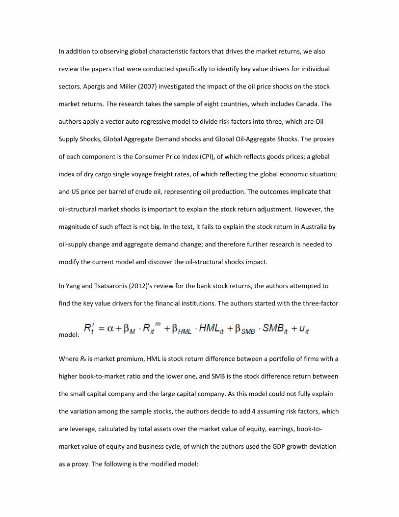
In Yang and Tsatsaronis (2012)’s review for the bank stock returns, the authors attempted to
find the key value drivers for the financial institutions. The authors started with the three-factor
model:
Where Rit is market premium, HML is stock return difference between a portfolio of firms with a
higher book-to-market ratio and the lower one, and SMB is the stock difference return between
the small capital company and the large capital company. As this model could not fully explain
the variation among the sample stocks, the authors decide to add 4 assuming risk factors, which
are leverage, calculated by total assets over the market value of equity, earnings, book-to-
market value of equity and business cycle, of which the authors used the GDP growth deviation
as a proxy. The following is the modified model:

The data included the annual stock returns of 50 actively traded global banks over 11 OECD
countries. The result demonstrated all the additional risk factors are meaningful and conclude
that higher leverage ratio would lead to lower stock returns. Moreover, higher capital
requirements can be beneficial to stock holders.
Another studied completed by King (2009) demonstrated a CAPM approach to estimate the cost
of equity for global banks. The author first highlighted the fact that after the 2008 financial crisis,
the importance of the Tier 1 Capitals should be more carefully considered in the evaluation. The
common equity is the first category of bank capital available to absorb losses; therefore
investors would expect to be rewarded for the greater risk they bear. Hence the common equity
should be the most expensive form of the bank capital.
The author then took the single factor CAPM approach to try to estimate the cost of equity for
global banks headquartered in the major countries including Canada and the U.S., with data set
from 1990 to 2009. The study discovered that the real cost of equity decreased steadily across
all countries except Japan from 1990 to 2006 but then rose from 2006 onwards. There were
clear cyclical patters for each country, which increases the cost of equity of the banking sector in
around 1994 and 2000. The author discovered that approximately one-third of the portion of
the decrease in the cost of equity reflects the decrease in the risk-free rates, while two-thirds of
the portion of the decrease of the cost of equity was explained by the banking sector risk
premium. This research also demonstrated a wide variation results across banks indicating the
difficulties of estimating the expected return by single factor CAPM mode.

The following two articles are the literatures that we solely based on research on. Dimson,
Marsh, and Staunton (2011) updated global estimates of historical ERP that were previously
modeled by other academics. The research included 19 countries including Canada, and the
dataset included equities, long term bonds, bills, inflation, exchange rates, and GDP, from 1900
to 2010. The findings indicated that equity outperformed bonds, bills, and inflation during the
past 110 years, both in nominal terms and in real terms. The article then decomposes ERPs on
geometric average for 19 countries, demonstrated a 4.94% and 5.26% for Canada and the U.S.
respectively. This premium calculated were broken down into 5 factors, namely Geometric
Mean Dividend Yield, Dividend Growth Rate, Change of Price-to-Dividend Ratio, Real Exchange
Rate, and US Real Interest Rate. The article concluded that the investors should expect a long-
run equity premium (relative to bills) of around 3.0-3.5% on a geometric mean basis, and an
arithmetic mean premium for the World index of approximately 4.5-5.0%.
Lastly, we also examined an article by Grinold, Kroner, and Siegel (2011) to get a different
perspective of how we may approach the ERP estimation problem. In this article, the authors
first noted that there was no clear method on how to measure ERP historically. They highlighted
Grinold and Kroner (2002) proposed an alternative model for the ERP that linked the return
closely to GDP growth. The main reason behind this model was due to the fact that the authors
believe any of the company cannot sustain to grow too fast or too slow compared to the GDP.
The Grinold and Kroner model that the authors applied broke down the expected return of
equity over a period into 3 factors, namely Income, Earnings Growth, and Re-Pricing Factors. As
the authors discovered in their research, the ERP that Grinold and Kroner model suggested back
in 2002, evaluated over 2002-2011, was too high. The recent update in 2011 with the existing
model, the ERP estimated over the 10-year treasuries is 3.6%. The main issue came from the
volatile re-pricing factor, of which was simply the change of the Price-to-Earnings ratio.

Therefore the authors concluded that they were not fully confident with their ERP forecast
based on the Grinold and Kroner model, but rather they believe this model can provide a
reasonable range for referencing purpose.
Analysis
As discussed in the introduction, the main focus of the ERP analysis underlies in understanding
what factors that drives the market returns; since we have determined ERP as the expected
market (or sector) returns minus the Canadian 10 Year Federal Government Bond Rate. In the
attempt to analyze the factors that drives the historic market return, we first attempt to
replicate the approach conducted by Dimson et al (2011). In Dimson model, the authors used
the following factors to decompose the historical market returns:
Estimated Return of the Market = Geometric Mean Dividend Yield + Dividend Growth Rate +
Change of Price-to-Dividend Ratio + Real Exchange Rate
Since this research is conducted to analyze the U.S. market, we slightly modified the data. The
database construction and the result of the replication will be discussed in the section below.

3.1 Database Construction
Since we want to understand the Canadian large-cap market within the context of the SIAS IPS,
we focus our research on large-cap Canadian equity markets, of which we have selected S&P
TSX 60 Index as our base market return proxy. All of our data used in this research are monthly
data observed from 2000/01/01 to 2012/06/30, and therefore any returns and/or growth rates
are annualized, gathered on a monthly basis. For example, the return of a single stock on
2012/06/30 is calculated by the price appreciation from 2011/06/30 to 2012/06/30 plus the
dividend paid during this time period, if any. To simplify the study, we assumed there is no
reinvestment of the dividends received in the same security. We chose this timer period of 150
months of data for two main reasons: first we want to observe the data that is available to us
that can allow us to replicate the studies that were conducted before; and secondly we want to
ensure that the data include the most current financial crisis so that we are capturing the affect
of the crisis on the market as well. We believe that 150 months of data is sufficient enough to
capture at least a business cycle for a cyclical company for the most cases. The sources for our
database included Bloomberg terminal, ThomsonOne terminal, Federal Reserve Economic
Data (FRED), and Yahoo! Finance. The detailed database description can be found in Appendix A.
Due to the fact that the Canadian stock market in general is heavily weighted in the major three
sectors (namely energy sector, material sector, and financial sector), we have decided to break
down S&P TSX 60 further, and pull out the sub sector stocks in these three sectors to construct
our own sector indices. We have constructed the sub-sector indices with the market-weight
method for the consistency with the S&P TSX 60 Index.
Below is a summary of the indices that we will be using in this equity return analysis.
S&P TSX 60 Index

With the reasoning stated above, this Index will be used as a proxy for our Canadian stock
market returns.
Sub-Sector Indices (Energy, Material & Financial)
These market-weight indices are constructed by pulling out the company listings as of June 30th,
2012 from S&P TSX 60, and given market weight for each of the stock listing, to compute a
market weighted return index. We have encountered some listings that were not listed for the
entire time period as the stock listing can vary between time periods; however this does not
alter our indices since the replacement stocks’ behaviours are closely correlated to the replaced
stocks. Our main focus was to generate a sub-sector index that can be representative of the
large-cap market for that specific index as the SIAS IPS constraints us to, and we believe the
substitutions of the stock throughout the time period does not affect our focus. Therefore we
have decided to keep the current TSX 60 listings as our base for the purpose of research.
The Key Drivers Used in the Analysis
The Appendix A shows the variables that will be tested in our analysis. We have selected our
variables in a way to represent any of the studies that we meant to replicate. For example,
Dimson model highlighted Geometric Mean Dividend Yield, Dividend Growth Rate, Change of
Price-to-Dividend Ratio, and Real Exchange Rate as key variables, and we classified these
variables as Dimson Model factors under the “Variable Classification” section. In addition, we
also want to analyze what are the other macro data that may be affecting the market’s returns.
As a variation of the Grinold’s model, we broke down the GDP function as GDP = C+I+G+(X-M).
We try to find reasonable representative proxies for each and every one of the factors in the
equation in our analysis. While we would like to use as many economic proxies as possible, we
are also aware that we want to focus on monthly data that will be available to us. Therefore our
selection was limited but at the same time representative to key economy drivers. These
variables are classified with its representative proxies of the GDP function under the “Variable
Classification” section. Lastly, for the variables that we believe that a shocking factor to affect
the market returns, we classify these variables as Shock factors under the “Variable
Classification” section.
3.2 Methodology
Our methodology to identify key factors that drives the market returns can be separates into
three stages. In stage one, the single variables listed in the Appendix A is regressed against the
targeted market or sub-sector return. We apply a 95% confidence level, and therefore we
expect any variable as significant when its t-test’s p-value is less than or equal to 5%. In addition,
we consider any variable might be significant, and may need further research on, when its t-
test’s p-value is between 5% - 20%.
In the second stage of the research, we pull the statistically significant variables identified from
the stage one of the analysis, group them together, to run the regression against the targeted
market or sub-sector return. During this stage, the variables are reviewed whether any co-
linearity issue exists, as we perceived any correlation of ±50% or above of any two variables
should be cautiously evaluated.
The final stage of the research is the look at the result from stage two, and trim down the non-
statistically significant variables. Again here we apply a 95% confidence level. The multi-factor
model will be trimmed down until all the variables are statistically significant at 95% confidence
level. Depends on the multi-factor model’s result, we may perceive a variable might be a
significant driver should its t-test’s p-value falls between 5%-20%.

3.3 The Result of Replication of Dimson Model
As discussed earlier, before we attempt to step in to identify the key factors that drive market
return, we attempt to replicate the Dimson Model with the Canadian data. Again, in Dimson
model, the authors used the following factors to estimate the return of the market:
Estimated Return of the Market = Geometric Mean Dividend Yield + Dividend Growth Rate +
Change of Price-to-Dividend Ratio + Real Exchange Rate
We have observed the similar data based off S&P TSX 60 Index, with its respectively market-
weighted dividend yield, dividend growth rate, change of trailing twelve months price-to-
dividend ratios, and inflation adjusted real exchange rates between CAD and USD.
Surprisingly, the variables identified by Dimson have strong abilities to estimate the market
returns, as the regression result demonstrated below:
Table 1. The Dimson Model Replication Result R Square: 97.75% Coefficients Standard Error t Stat P-value Geographic Mean Dividend Yield -0.01246397 0.028630622 -0.435337047 66.40% Real SPTSX 60 Dividend Growth 0.930277886 0.021481826 43.30534424 0.00% Change of P/D 0.958074009 0.014757749 64.92006459 0.00% Change in Real Exchange Rate -0.120046678 0.024759226 -4.848563375 0.00%
Table 1 demonstrated that the four variables together explained approximately 98% of the total
market return. We found this result fascinating and we were confident to implement Dimson’s
finding into our analysis in attempt to further identify more variables that may assist in
expressing Canadian large-cap equity markets’ returns.

4.1 S&P TSX 60 Return Modeling
4.1.1 Single Variable Screening
Table 2 below is a summary for the variables that we have selected as our starting point for
analyzing returns of S&P TSX 60 Index. As stated earlier, each and everyone one of the variables
were selected under the classification as whether the variables came from Dimson model, the
GDP growth factors, or a shock factor that we believe had the potential to be influence in our
multi-factor model. We ran an annualized data observed on a monthly basis regression against
the historic S&P TSX 60 return with each and every one of the variables listed in Appendix A to
see how significant the variable is at the 95% level of confidence level and also whether the sign
of the coefficient matches our expectation. At the same time we carefully examine co-linearity
issue by making sure the variables that we use in the models do not have ±50% of correlation or
higher. We identify a variable that may be significant enough to be tested in our multi-factor
model if the T-Test P-Value is ranged from 0%-20%, and the consistent sign of coefficients
compared to our expectations.

Table 2. The Initial Screening of the Key Variables – S&P TSX 60 Returns Variable Name Variable Classification R-Square Coef Exp Coef T Test P-Value Significance
Geographic Mean Dividend Yield Dimson Model 2.29% - + 6.52% Maybe
Real SPTSX 60 Dividend Growth Dimson Model 0.13% + + 66.62% No
Change of P/D Dimson Model 63.73% + + 0.00% Yes
Change in Real Exchange Rate Dimson Model 31.70% - - 0.00% Yes
Gold Price Return Shock 0.03% - - 83.44% No
Copper Price Return Shock 2.36% + + 6.16% Maybe
Oil Price Return Shock 7.58% + + 0.07% Yes
Gas Price Return Shock 3.08% + + 3.22% Yes
Canada Unemployment Rate Growth C 0.00% + - 89.34% No
Canada PMI Return I 0.65% - + 32.81% No
Global PMI Return I 10.00% + + 0.01% Yes
Dry Baltic Return X-M 6.08% + + 0.24% Yes
Canada Treasury Bill Rate Return C 0.00% + - 72.05% No
Canada 10 Year - 30 Day Bond Rate Return C 0.11% - + 68.08% No
USD/Euro Rate Growth X-M 7.28% + + 0.09% Yes
CAD/USD Rate Growth X-M 12.83% - - 0.00% Yes
JAP/USD Rate Growth X-M 2.98% + + 3.54% Yes
AA Corporate Bond Index Return Shock 1.67% + + 11.62% Maybe
BBB+ Corporate Bond Index Return Shock 7.25% + + 0.09% Yes
US Housing Starts Growth C 0.00% + + 81.47% No
US Unemployment Rate Growth C 0.13% - - 66.33% No
SP TSX 60 P/E Growth Re-Pricing 55.34% + + 0.00% Yes
SP TSX 60 P/B Growth Re-Pricing 83.95% + + 0.00% Yes
US CPI Growth C 2.46% + + 5.63% Maybe
US Import Goods From Canada Growth X-M 0.87% + + 25.67% No
US Import Goods To Canada Growth X-M 0.72% + + 30.49% No
VIX Return Shock 39.90% - - 0.00% Yes
Tier 1 Capital Return Shock 0.00% - + 89.09% No
As demonstrated, we have selected the 28 variables that we believe have the potential to drive
the Canadian large-cap equity markets’ returns. The detail description and the source of the
variables can be found in Appendix A.
In addition to the four key variables identified by the Dimson model, we believe the commodity
prices are the shock factors that can be brought to the Canadian equity market, as Apergis and
Miller demonstrated regarding to oil price shocks. Three of the four variables have consistent
coefficients as expected with low t-test p-value, and therefore these variables will be selected
for multi-factor modeling.

We expect the Canadian unemployment rates and Treasury bill rates, as well as the US
unemployment rates, housing starts, and CPI are proxies for the consumption factor of the
Canadian economy; however we were only able to observe that the US CPI might be a value
driver for the market return.
We also examine the Canada PMI and Global PMI as the gross investment factor of GDP proxies,
since the PMIs represent productivities of a country. We would like to highlight that due to the
unavailability of gathering data for China’s PMI back to 2000/01/01, we use the existing 5-year
data and tested the correlation between China’s PMI with Global PMI. What we have discovered
was the two PMIs have almost 70% of correlation. Therefore in this paper we will use Global
PMI as a proxy for China’s PMI. As Table 2 demonstrated, the Global PMI is statistically
significant, and therefore will be tested in the multi-factor model.
We would also like to use the exchanges rates, as well as Dry Baltic Index, as proxies for the X-M
factor of the GDP model, and whether these factors have any effect on the Canadian market
return. In addition, we were also using the import/export data between US and Canada as other
proxies for the X-M factor. As Table 2 suggested, we will put the Dry Baltic Index and the
exchange rates into our multi-factor modeling.
Lastly, with a slight variation of the Grinold model’s Re-Pricing factor, we have implemented two
potential Re-Pricing factors as the change of the TSX 60 Index T12M P/E and T12M P/B into our
analysis. We have also observed two more potential shock factors as the VIX Index, which
reflects the volatility index of the US market; and the market-weighted average of the major
Canadian Banks’ Tier 1 Capital Ratio, which represent the leverage factor studied by both Yang
and King. The addition of the AA and BBB+ Corporate Bond Index represent variables that we
think that might have the surprise factor as it represent the performance of US dollar
denominated investment grade rated corporate debt publically issued in the US domestic
market. We believe that by adding these Bond Indices will assist us to identify whether the
Canadian market returns are correlated to the US economy factors. Table 2 shows that both of
the Re-Pricing factors, both of the Bond Indices, and the VIX Index should be included into our
second stage of multi-factor modeling.
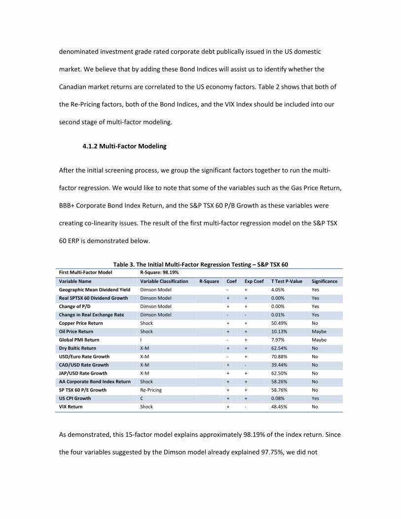
4.1.2 Multi-Factor Modeling
After the initial screening process, we group the significant factors together to run the multi-
factor regression. We would like to note that some of the variables such as the Gas Price Return,
BBB+ Corporate Bond Index Return, and the S&P TSX 60 P/B Growth as these variables were
creating co-linearity issues. The result of the first multi-factor regression model on the S&P TSX
60 ERP is demonstrated below.
Table 3. The Initial Multi-Factor Regression Testing – S&P TSX 60 First Multi-Factor Model R-Square: 98.19%
Variable Name Variable Classification R-Square Coef Exp Coef T Test P-Value Significance
Geographic Mean Dividend Yield Dimson Model - + 4.05% Yes
Real SPTSX 60 Dividend Growth Dimson Model + + 0.00% Yes
Change of P/D Dimson Model + + 0.00% Yes
Change in Real Exchange Rate Dimson Model - - 0.01% Yes
Copper Price Return Shock + + 50.49% No
Oil Price Return Shock + + 10.13% Maybe
Global PMI Return I - + 7.97% Maybe
Dry Baltic Return X-M + + 62.54% No
USD/Euro Rate Growth X-M - + 70.88% No
CAD/USD Rate Growth X-M + - 39.44% No
JAP/USD Rate Growth X-M + + 62.50% No
AA Corporate Bond Index Return Shock + + 58.26% No
SP TSX 60 P/E Growth Re-Pricing + + 58.76% No
US CPI Growth C + + 0.08% Yes
VIX Return Shock + - 48.45% No
As demonstrated, this 15-factor model explains approximately 98.19% of the index return. Since
the four variables suggested by the Dimson model already explained 97.75%, we did not
perceive this model is significantly better than the Dimson model. For the final stage of the
analysis to extend on the testing, we took out the variables that were not significant, and re-run
the regression again.
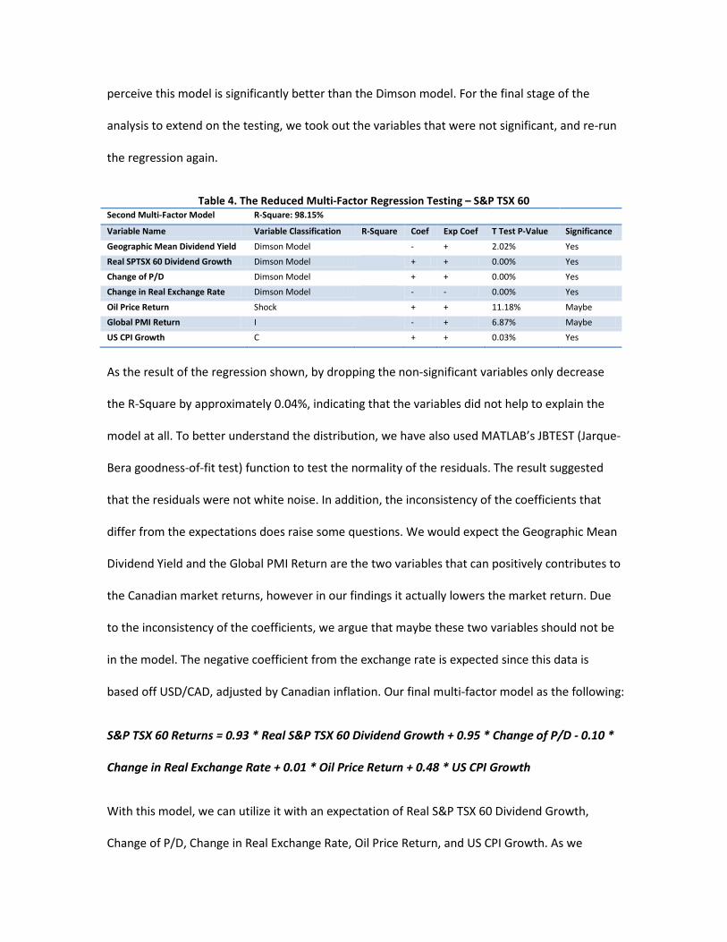
Table 4. The Reduced Multi-Factor Regression Testing – S&P TSX 60 Second Multi-Factor Model R-Square: 98.15%
Variable Name Variable Classification R-Square Coef Exp Coef T Test P-Value Significance
Geographic Mean Dividend Yield Dimson Model - + 2.02% Yes
Real SPTSX 60 Dividend Growth Dimson Model + + 0.00% Yes
Change of P/D Dimson Model + + 0.00% Yes
Change in Real Exchange Rate Dimson Model - - 0.00% Yes
Oil Price Return Shock + + 11.18% Maybe
Global PMI Return I - + 6.87% Maybe
US CPI Growth C + + 0.03% Yes
As the result of the regression shown, by dropping the non-significant variables only decrease
the R-Square by approximately 0.04%, indicating that the variables did not help to explain the
model at all. To better understand the distribution, we have also used MATLAB’s JBTEST (Jarque-
Bera goodness-of-fit test) function to test the normality of the residuals. The result suggested
that the residuals were not white noise. In addition, the inconsistency of the coefficients that
differ from the expectations does raise some questions. We would expect the Geographic Mean
Dividend Yield and the Global PMI Return are the two variables that can positively contributes to
the Canadian market returns, however in our findings it actually lowers the market return. Due
to the inconsistency of the coefficients, we argue that maybe these two variables should not be
in the model. The negative coefficient from the exchange rate is expected since this data is
based off USD/CAD, adjusted by Canadian inflation. Our final multi-factor model as the following:
S&P TSX 60 Returns = 0.93 * Real S&P TSX 60 Dividend Growth + 0.95 * Change of P/D - 0.10 *
Change in Real Exchange Rate + 0.01 * Oil Price Return + 0.48 * US CPI Growth
With this model, we can utilize it with an expectation of Real S&P TSX 60 Dividend Growth,
Change of P/D, Change in Real Exchange Rate, Oil Price Return, and US CPI Growth. As we

expect to have the number as 0.85%, -0.66%, -0.24%, 0.74%, and 0.20% respectively, we have an
expected annualized S&P TSX 60 Return of 4.82%, in the month of August, 2012. This leads us to
calculate the annualized ERP for the Canadian large-cap equity market as 4.82% - 1.25% = 3.57%.
This result is actually extremely close compared to Dimson’s model, of which the arithmetic
mean premium for the world index at 4.5%-5.0% and the long-run equity premium on geometric
mean basis of 3.0%-3.5%; and also match up with Grinold’s model quite nicely as our 3.57% of
ERP is basically right on with Grinold’s 3.6% result. However, as we used the betas for each of
the variables to backtrack the ERP throughout the entire time period, we have observed that the
risk free rate had been outperforming the return of the market, as the historic ERP
demonstrated a -2.35%, with a 4.80% of standard deviation.
In order to examine if there exist any of the co-linearity issue, we have also performed a
correlation matrix to see if there exists high correlation (±50% or above) between these
variables. The result of the findings is demonstrated in Table 5.
Table 5. The Correlation Matrix for the Significant Variables
Real SPTSX 60
Dividend Growth Change of
P/D
Change in Real
Exchange Rate
Oil Price Return
US CPI Growth
Real SPTSX 60 Dividend Growth 100.00% Change of P/D -55.82% 100.00%
Change in Real Exchange Rate 2.75% -44.68% 100.00% Oil Price Return -14.84% 27.84% -22.49% 100.00%
US CPI Growth -7.50% 12.22% -12.58% 58.01% 100.00% As demonstrated, we should be concerned with a few variables as the correlations between the
Real S&P TSX 60 Dividend Growth and the Change of P/D, as well as the correlation between the
Oil Price Return and the US CPI Growth have relatively high correlations as these numbers
surpassed our comfort threshold. We believe further analysis is needed to understand the
relationships between these variables better.

4.2 Energy Sub-Sector Index Return Modeling
4.2.1 Single Variable Screening
After our attempt to determine what are the value drivers for the general large-cap market
return, our focus then turns to a more specific sub-sector returns, as the Canadian equity
markets are mainly consist of three major sectors. We construct the sub-sector index from the
TSX 60 listed energy sector companies as of June 30th, 2012 by a market-weighted average of
total appreciation to calculate the sub-sector returns; and also using the same method to
calculate the dividend yields. The time periods of the data for the sub-sectors were observed
from 2000/01/01 to 2012/06/30. Following are the variables for our regression testing:
Table 6. The Initial Screening of the Key Variables – Energy Variable Name (Total Return) Variable
Classification R-Square Coef
Exp Coef
T Test P-Value Significance
S&P TSX 60 Return Dimson Model 41.44% + + 0.00% Yes Energy Sector Dividend Growth Dimson Model 21.68% - - 0.00% Yes Gold Price Return Shock 0.25% - + 54.57% No Copper Price Return Shock 1.94% + + 9.03% Maybe Oil Price Return Shock 10.27% + + 0.01% Yes Gas Price Return Shock 3.53% + + 2.17% Yes Canada Unemployment Rate Growth C 0.80% - - 27.71% No Canada PMI Return I 0.00% - + 92.86% No Global PMI Return I 4.41% + + 1.01% Yes Dry Baltic Return X-M 3.00% + + 3.44% Yes Canada Treasury Bill Rate Return C 0.72% + - 30.23% No Canada 10 Year - 30 Day Bond Rate Return C 1.48% - + 14.01% Maybe USD/Euro Rate Growth X-M 2.93% + + 3.67% Yes CAD/USD Rate Growth X-M 7.08% - - 0.10% Yes JAP/USD Rate Growth X-M 2.65% + - 4.74% Yes AA Corporate Bond Index Return Shock 0.57% + + 36.07% No BBB+ Corporate Bond Index Return Shock 2.23% + + 6.90% Maybe US Housing Starts Growth C 0.23% + + 56.40% No US Unemployment Rate Growth C 1.43% - - 14.64% Maybe SP TSX 60 P/E Growth Re-Pricing 21.72% + + 0.00% Yes SP TSX 60 P/B Growth Re-Pricing 39.25% + + 0.00% Yes US CPI Growth C 2.04% + + 8.26% Maybe US Import Goods From Canada Growth X-M 0.01% + + 88.90% No US Import Goods To Canada Growth X-M 0.20% + + 59.11% No VIX Return Shock 17.13% - - 0.00% Yes Tier 1 Capital Return Shock 0.26% - + 54.01% No

First and foremost, we assume that the return of the sub-sector index is a function of the overall
market return, plus the sector-specific variables that drives the market. Therefore, our very first
variable that we would like to include is the overall S&P TSX 60 Return. The rest of the variables
were exactly the same variables that were tested in the earlier analysis. Note that instead of the
S&P TSX 60’s overall dividends, we have constructed our own sub-sector index’s market-
weighted dividend yield and its growth rate to replace it. Again after completing the first stage
of the initial screening process to identify individual value drivers for sub-sector returns, we
move on to second stage of the analysis which is multi-factor regression modeling.
4.2.2 Multi-Factor Modeling
With the same selection method as previously discussed, we have grouped the variables
together to perform a multi-factor regression.
Table 7. The Initial Multi-Factor Regression Testing – Energy First Multi-Factor Model (Total Return) R-Square: 54.63% Variable Name Variable
Classification R-Square Coef Exp Coef T Test P-Value Significance
S&P TSX 60 Return Dimson Model
+ + 0.00% Yes Energy Sector Dividend Growth Dimson Model
- - 0.00% Yes
Oil Price Return Shock
+ + 62.26% No Gas Price Return Shock
+ + 17.29% Maybe
Canada Unemployment Rate Growth Shock
+ + 70.39% No Canada Treasury Bill Rate Return I
- + 47.75% No
Canada 10 Year - 30 Day Bond Rate Return X-M
+ + 56.87% No
JAP/USD Rate Growth C
- - 14.73% Maybe BBB+ Corporate Bond Index Return X-M
+ + 81.62% No
US Unemployment Rate Growth X-M
- - 87.96% No SP TSX 60 P/B Growth X-M
+ + 57.64% No
US CPI Growth Shock
- + 19.24% Maybe Tier 1 Capital Return C
- - 33.63% No
As demonstrated, only 2 out of the 13 variables are significant at 95% confidence, while three
variables are close to being significant. This model explains approximately 55% of the market-
weighted energy sector return. By trimming the non-significant variables, we have the following:

Table 8. The Reduced Multi-Factor Regression Testing – Energy Second Multi-Factor Model (Total Return) R-Square: 51.87%
Variable Name Variable Classification
R-Square Coef Exp Coef T Test P-Value
Significance
S&P TSX 60 Return Dimson Model + + 0.00% Yes
Energy Sector Dividend Growth Dimson Model - - 0.00% Yes
Oil Price Return Shock + + 5.04% Yes
By decreasing the number of variables down to 3, we only lost less than 3% of explanations of
the model. We were quite satisfied with the result as the three factor model explained
approximately 52% of the entire sub-sector returns, with all of the coefficient signs align with
our expectations. In regards to the residuals, according to the result of the JBTEST from MATLAB,
the residuals are not white noise. With the remaining four variables are all significant, we have
concluded our multi-factor model as below:
Energy Sector Return = 0.61 * S&P TSX 60 Return – 0.13 * Energy Sector Dividend Growth +
0.07 * Oil Price Return
With our expectation of 4.82% of the S&P TSX 60 Return, 0.60% of Energy Sector Dividend
Growth, and 0.74% of the Oil Price Return, we estimated the Energy Sector Return to be
approximately 2.91%; of which lead us to conclude that the annualized Energy Sector ERP for
the month of August is estimated at 2.91% - 1.25% = 1.66%. The regression historic Energy
Sector ERP is averaged at -2.50% with a 4.12% of standard deviation. We did not find this result
insulting as it demonstrated a similar behaviour with the S&P TSX 60 ERP. We have also
discovered no co-linearity issue between the variables, as shown in Table 9.
Table 9. The Correlation Matrix for the Significant Variables SPTSX60 Return Energy Dividend Growth Oil Price Return
SPTSX60 Return 100.00% Energy Dividend Growth -25.68% 100.00%
Oil Price Return 27.52% -20.53% 100.00%
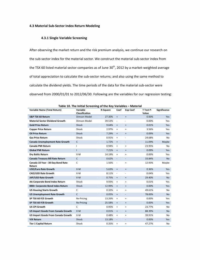
4.3 Material Sub-Sector Index Return Modeling
4.3.1 Single Variable Screening
After observing the market return and the risk premium analysis, we continue our research on
the sub-sector index for the material sector. We construct the material sub-sector index from
the TSX 60 listed material sector companies as of June 30th, 2012 by a market-weighted average
of total appreciation to calculate the sub-sector returns; and also using the same method to
calculate the dividend yields. The time periods of the data for the material sub-sector were
observed from 2000/01/01 to 2012/06/30. Following are the variables for our regression testing:
Table 10. The Initial Screening of the Key Variables – Material Variable Name (Total Return) Variable
Classification R-Square Coef Exp Coef T Test P-
Value Significance
S&P TSX 60 Return Dimson Model 27.30% + + 0.00% Yes
Material Sector Dividend Growth Dimson Model 39.53% - - 0.00% Yes
Gold Price Return Shock 9.64% + + 0.01% Yes
Copper Price Return Shock 2.97% + + 3.56% Yes
Oil Price Return Shock 7.29% + + 0.09% Yes
Gas Price Return Shock 0.91% + - 24.68% No
Canada Unemployment Rate Growth C 1.72% + - 11.09% Maybe
Canada PMI Return I 0.94% + + 23.95% No
Global PMI Return I 7.21% + + 0.09% Yes
Dry Baltic Return X-M 14.19% + + 0.00% Yes
Canada Treasury Bill Rate Return C 0.62% - - 33.84% No
Canada 10 Year - 30 Day Bond Rate Return
C 1.56% - + 12.93% Maybe
USD/Euro Rate Growth X-M 5.63% + + 0.36% Yes
CAD/USD Rate Growth X-M 8.11% - - 0.04% Yes
JAP/USD Rate Growth X-M 0.75% + + 29.40% No
AA Corporate Bond Index Return Shock 9.93% + + 0.01% Yes
BBB+ Corporate Bond Index Return Shock 12.99% + + 0.00% Yes
US Housing Starts Growth C 0.32% + + 49.61% No
US Unemployment Rate Growth C 0.05% + - 78.00% No
SP TSX 60 P/E Growth Re-Pricing 13.26% + + 0.00% Yes
SP TSX 60 P/B Growth Re-Pricing 25.58% + + 0.00% Yes
US CPI Growth C 0.95% + + 23.77% No
US Import Goods From Canada Growth X-M 0.01% + + 88.39% No
US Import Goods From Canada Growth X-M 0.48% + + 39.91% No
VIX Return Shock 13.18% - - 0.00% Yes
Tier 1 Capital Return Shock 0.35% + + 47.27% No
Again, we assume that the return of the material sub-sector index is a function of the overall
market return, plus the material sector-specific variables that drives the market. Therefore, our
very first variable that we would like to include is the overall S&P TSX 60 Return. The rest of the
variables were exactly the same variables that were tested in the earlier analysis. Note that
instead of the energy sub-sector dividends, we have constructed the material sub-sector index’s
market-weighted dividend yield and its growth rate to replace it. Again after completing the first
stage of the initial screening process to identify individual value drivers for the material sub-
sector returns, we move on to second stage of the analysis.
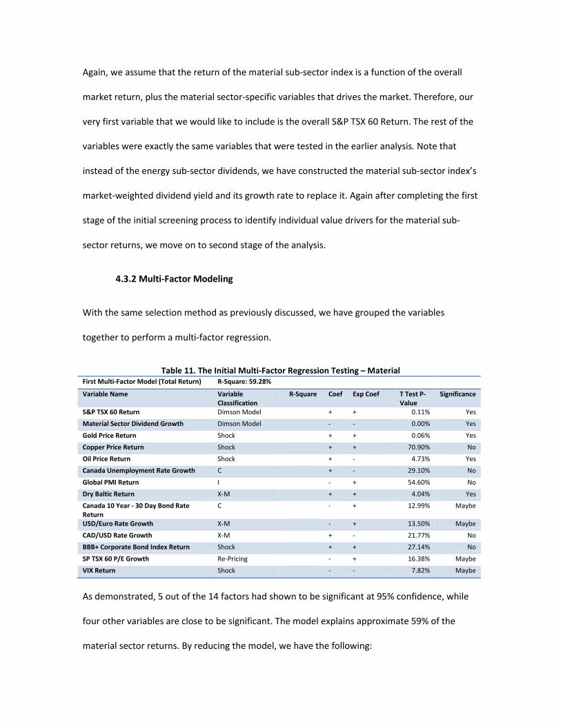
4.3.2 Multi-Factor Modeling
With the same selection method as previously discussed, we have grouped the variables
together to perform a multi-factor regression.
Table 11. The Initial Multi-Factor Regression Testing – Material First Multi-Factor Model (Total Return) R-Square: 59.28%
Variable Name Variable Classification
R-Square Coef Exp Coef T Test P-Value
Significance
S&P TSX 60 Return Dimson Model + + 0.11% Yes
Material Sector Dividend Growth Dimson Model - - 0.00% Yes
Gold Price Return Shock + + 0.06% Yes
Copper Price Return Shock + + 70.90% No
Oil Price Return Shock + - 4.73% Yes
Canada Unemployment Rate Growth C + - 29.10% No
Global PMI Return I - + 54.60% No
Dry Baltic Return X-M + + 4.04% Yes
Canada 10 Year - 30 Day Bond Rate Return
C - + 12.99% Maybe
USD/Euro Rate Growth X-M - + 13.50% Maybe
CAD/USD Rate Growth X-M + - 21.77% No
BBB+ Corporate Bond Index Return Shock + + 27.14% No
SP TSX 60 P/E Growth Re-Pricing - + 16.38% Maybe
VIX Return Shock - - 7.82% Maybe
As demonstrated, 5 out of the 14 factors had shown to be significant at 95% confidence, while
four other variables are close to be significant. The model explains approximate 59% of the
material sector returns. By reducing the model, we have the following:

Table 12. The Reduced Multi-Factor Regression Testing – Material Second Multi-Factor Model (Total Return) R-Square: 55.63%
Variable Name Variable Classification
R-Square Coef Exp Coef T Test P-Value
Significance
S&P TSX 60 Return Dimson Model + + 0.17% Yes
Material Sector Dividend Growth Dimson Model - - 0.00% Yes
Gold Price Return Shock + + 0.01% Yes
Dry Baltic Return X-M + + 1.33% Yes
VIX Return Shock - - 9.57% Maybe
The above five-factor model explains approximately 56% of the material sector return, which we
were quite satisfied with. In regards to the residuals, according to the result of the JBTEST from
MATLAB, the residuals are not white noise. All of the variables are significant in the 95%
confidence level, with the expected coefficient signs equal to the results; we have concluded our
multi-factor model as below:
Material Sector Return = 0.45 * S&P TSX 60 Return – 0.22 * Material Sector Dividend Growth +
0.51 * Gold Price Return + 0.06 * Dry Baltic Return – 0.06 * VIX Return
With our expectation of 4.82% of the S&P TSX 60 Return, 1.50% of the Material Sector Dividend
Growth, 1.00% of the Gold Price Return, 5.00% of the Dry Baltic Return, and -5.00% of the VIX
Return, we estimate the annualized Material Sector Return at 2.95%; of which lead to the
annualized Material Sector ERP at 2.95% - 1.25% = 1.70%. The Material Sub-Sector’s historical
regression ERP was higher than the energy sector one, yet more volatile, as the historical
averages out to be -1.95%, with a 6.66% of standard deviation. We have also discovered the
possibility of the co-linearity issue between the VIX Index and the S&P TSX 60 Return, as the
table below demonstrated that the correlation between these two variables is -63%. If needed,
we will be comfortable to take the VIX Return variable out of the model as it does not meet the
95% confidence level’s significance requirement; but rather it is only significant at 90% of the
confidence level.

Table 13. The Correlation Matrix for the Significant Variables
SPTSX60 Return
Material Dividend Growth
Gold Price Return
Dry Baltic Return VIX Return
SPTSX60 Return 100.00% Material Dividend Growth -40.95% 100.00%
Gold Price Return -1.73% -24.65% 100.00% Dry Baltic Return 24.66% -23.48% 21.21% 100.00%
VIX Return -63.17% 26.17% 21.99% -17.65% 100.00%
4.4 Financial Sub-Sector Index Return Modeling
4.4.1 Single Variable Screening
Lastly, we continue to research the final sub-sector index for the financial sector. Again the
financial sub-sector index was constructed from the TSX 60 listed financial sector companies as
of June 30th, 2012 by a market-weighted average of total appreciation to calculate the sub-
sector returns; and also using the same method to calculate the dividend yields. The time
periods of the data for the financial sub-sector were observed from 2000/01/01 to 2012/06/30.
Following are the variables for our regression testing:

Table 14. The Initial Screening of the Key Variables – Financial Variable Name (Total Return) Variable
Classification R-Square Coef Exp Coef T Test P-
Value Significance
S&P TSX 60 Return Dimson Model 38.70% + + 0.00% Yes
Financial Sector Dividend Growth Dimson Model 90.12% - - 0.00% Yes
Gold Price Return Shock 2.70% - - 4.51% Yes
Copper Price Return Shock 1.80% + + 10.25% Maybe
Oil Price Return Shock 6.20% + - 0.22% Yes
Gas Price Return Shock 3.47% + - 2.29% Yes
Canada Unemployment Rate Growth C 2.13% - - 7.57% Maybe
Canada PMI Return I 0.00% + + 81.46% No
Global PMI Return I 19.54% + + 0.00% Yes
Dry Baltic Return X-M 2.58% + + 5.02% Maybe
Canada Treasury Bill Rate Return C 0.00% + - 87.71% No
Canada 10 Year - 30 Day Bond Rate Return
C 0.00% - + 97.16% No
USD/Euro Rate Growth X-M 2.23% + + 6.99% Maybe
CAD/USD Rate Growth X-M 9.07% - - 0.02% Yes
JAP/USD Rate Growth X-M 4.06% + + 1.37% Yes
AA Corporate Bond Index Return Shock 1.16% + + 19.03% Maybe
BBB+ Corporate Bond Index Return Shock 6.90% + + 0.12% Yes
US Housing Starts Growth C 0.08% + + 73.91% No
US Unemployment Rate Growth C 2.40% - - 5.87% Maybe
SP TSX 60 P/E Growth Re-Pricing 24.76% + + 0.00% Yes
SP TSX 60 P/B Growth Re-Pricing 42.69% + + 0.00% Yes
US CPI Growth C 2.61% + + 4.88% Yes
US Import Goods From Canada Growth
X-M 0.69% + + 31.51% No
US Import Goods From Canada Growth
X-M 0.69% + + 31.44% No
VIX Return Shock 24.37% - - 0.00% Yes
Tier 1 Capital Return Shock 1.26% + + 17.24% Maybe
Similarly, we assume that the return of the financial sub-sector index is a function of the overall
market return, plus the financial sector-specific variables that drives the market, of which may
or may not include the leverage factor – the Tier 1 Capital Return. Therefore, our very first
variable that we would like to include is the overall S&P TSX 60 Return. The rest of the variables
were exactly the same variables that were tested in the earlier analysis. Note that we have
constructed the financial sub-sector index’s market-weighted dividend yield and its growth rate
to replace the material dividend yields. Again after completing the first stage of the initial
screening process to identify individual value drivers for the financial sub-sector returns, we
move on to second stage of the analysis.

4.4.2 Multi-Factor Modeling
With the same selection method as previously demonstrated, we have grouped the variables
together to perform a multi-factor regression.
Table 15. The Initial Multi-Factor Regression Testing – Financial First Multi-Factor Model (Total Return) R-Square: 92.22%
Variable Name Variable Classification
R-Square Coef Exp Coef T Test P-Value
Significance
S&P TSX 60 Return Dimson Model + + 0.37% Yes
Financial Sector Dividend Growth Dimson Model - - 0.00% Yes
Gold Price Return Shock - - 10.73% Maybe
Copper Price Return Shock - + 71.02% No
Gas Price Return Shock + - 63.06% No
Canada Unemployment Rate Growth C - - 54.87% No
Global PMI Return I + + 16.25% Maybe
Dry Baltic Return X-M + + 27.74% No
USD/Euro Rate Growth X-M - + 87.66% No
CAD/USD Rate Growth X-M - - 95.27% No
JAP/USD Rate Growth X-M + + 76.32% No
BBB+ Corporate Bond Index Return Shock - + 33.95% No
US Unemployment Rate Growth C - - 14.15% Maybe
SP TSX 60 P/E Growth Re-Pricing + + 83.26% No
VIX Return Shock + - 80.75% No
Tier 1 Capital Return Shock + + 91.52% No
As demonstrated from Table 15, we have discovered a very interesting result. The total return of
the financial sector can be largely explained by 5 variables, with an impressive R-Square of 92%.
Moving forward, we reduce our multi-factor model to the significant value drivers:
Table 16. The Reduced Multi-Factor Regression Testing – Financial Second Multi-Factor Model (Total Return) R-Square: 92.04%
Variable Name Variable Classification
R-Square Coef Exp Coef T Test P-Value
Significance
S&P TSX 60 Return Dimson Model + + 0.00% Yes
Financial Sector Dividend Growth Dimson Model - - 0.00% Yes
Gold Price Return Shock - - 3.46% Yes
Global PMI Return I + + 6.55% Maybe
US Unemployment Rate Growth C - - 3.86% Yes
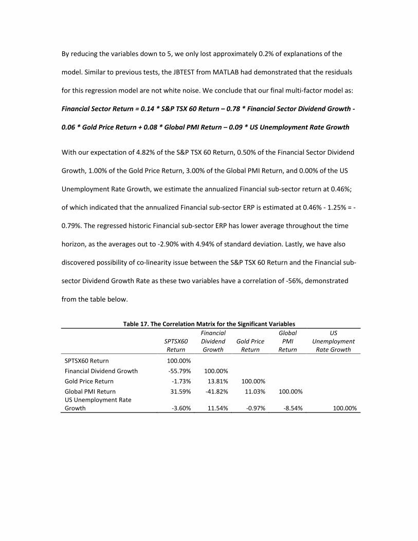
By reducing the variables down to 5, we only lost approximately 0.2% of explanations of the
model. Similar to previous tests, the JBTEST from MATLAB had demonstrated that the residuals
for this regression model are not white noise. We conclude that our final multi-factor model as:
Financial Sector Return = 0.14 * S&P TSX 60 Return – 0.78 * Financial Sector Dividend Growth -
0.06 * Gold Price Return + 0.08 * Global PMI Return – 0.09 * US Unemployment Rate Growth
With our expectation of 4.82% of the S&P TSX 60 Return, 0.50% of the Financial Sector Dividend
Growth, 1.00% of the Gold Price Return, 3.00% of the Global PMI Return, and 0.00% of the US
Unemployment Rate Growth, we estimate the annualized Financial sub-sector return at 0.46%;
of which indicated that the annualized Financial sub-sector ERP is estimated at 0.46% - 1.25% = -
0.79%. The regressed historic Financial sub-sector ERP has lower average throughout the time
horizon, as the averages out to -2.90% with 4.94% of standard deviation. Lastly, we have also
discovered possibility of co-linearity issue between the S&P TSX 60 Return and the Financial sub-
sector Dividend Growth Rate as these two variables have a correlation of -56%, demonstrated
from the table below.
Table 17. The Correlation Matrix for the Significant Variables
SPTSX60 Return
Financial Dividend Growth
Gold Price Return
Global PMI
Return
US Unemployment
Rate Growth
SPTSX60 Return 100.00% Financial Dividend Growth -55.79% 100.00%
Gold Price Return -1.73% 13.81% 100.00% Global PMI Return 31.59% -41.82% 11.03% 100.00%
US Unemployment Rate Growth -3.60% 11.54% -0.97% -8.54% 100.00%
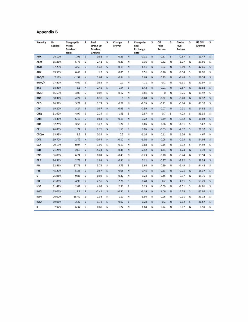
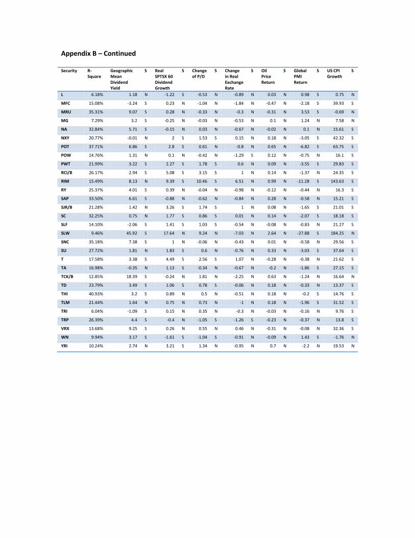
5.1 Implementation of the Findings
After completing the analysis on identifying the key value driver for the general Canadian large-
cap equity markets, we have implemented the result of the regression analysis on each and
every one of the stock listed in the TSX 60 Index as of June 30th, 2012. The result of the
regression is demonstrated in Appendix B. As the Appendix B shown, the fist column is for the
listed security code; second column is the result of the regression against that stock’s total
annualized monthly return; third, fifth, seventh, ninth, eleventh, and thirteenth columns are the
key value drivers identified from Section 4.1 The “S” right next to the variable indicates that
whether this variable was significant at 95% confidence level. Note that for the stocks that has
shorter time horizon of the return history, the regression was completed with only the existing
total returns. Therefore for some of the stocks, such as THI, for example, only ran a regression
with a sample size of 64, rather than 150.
The S&P TSX 60 Index multi-factor model has identified possible key factors or value drivers for
the annualized total return. Given the IPS constraint of the SIAS fund, we were not allowed to
short any of the individual security. However, assuming that we were able to do so, then we can
use this Appendix B to construct portfolios with securities that can hedge out any of the
exposures that we do not want to be exposed to by pairing long-short securities. For example, a
portfolio manager may want to reduce the risk exposure of factor one, while increasing the risk
exposure of factor two. Looking at Appendix B, we can identify the stocks with high risk
exposure to risk factor one and low risk exposure to factor two to sell, while purchasing the
stock with low exposure to risk factor one and high risk exposure to factor two.
6.1 Conclusion and Future Work
Inspired by the opportunity to perform equity valuation analysis for the SIAS fund, we have
attempted to identify key value drivers and risk factors that may affect the equity risk premium
for the Canadian large-cap equity markets. Our main focus was to develop regression models
that can perform reasonable estimation of equity risk premiums for the general large-cap
market, as well as the three major sectors in Canada.
Our framework was based on both of the Dimson’s model, as well as the GDP growth approach
developed by Grinold et al. While not all of the factors that we thought were important were
proven to be significant with the time horizon of the data from our selection, we did have some
success in developing multi-factor models. The results were quite satisfactory as the models are
demonstrating relatively high R-Squares, as match both of the Dimson and Grinold’s estimates
of the equity risk premiums. We strongly believe the models can be improved upon further
analysis in attempting to limit out the co-linearity issues, and this research provides a great
starting point for future cohorts who may have interest in further research into this topic.

Appendix
Appendix A
Variable Name Variable Classification Source Description
Geographic Mean Dividend Yield
Dimson Model Bloomberg The annualized mean dividend yield observed from TSX 60 Index
Real SPTSX 60 Dividend Growth
Dimson Model Bloomberg The annualized dividend growth rate is observed by the market-weighted average of the dividend growth rate
Change of P/D Dimson Model Bloomberg The annualized monthly incremental changes of the P/D ratio of the TSX 60 Index
Change in Real Exchange Rate
Dimson Model Bloomberg The annualized interest rate of CAD/USD adjusted by inflation
Gold Price Return Shock FRED The annualized gold price return
Copper Price Return Shock FRED The annualized copper price return
Oil Price Return Shock FRED The annualized oil price return
Gas Price Return Shock FRED The annualized gas price return
Canada Unemployment Rate Growth
C FRED The annualized change of Canada Unemployment Rate
Canada PMI Return I Bloomberg The annualized change of Canada PMI
Global PMI Return I Bloomberg The annualized change of Global PMI
Dry Baltic Return X-M Bloomberg The annualized change of the Dry Baltic Index
Canada Treasury Bill Rate Return
C FRED The annualized change of the Treasury Bill Rate
Canada 10 Year - 30 Day Bond Rate Return
C FRED The annualized change of the difference between 10 Year and 30 day Bond Rates
USD/Euro Rate Growth X-M FRED The annualized change of the USD/Euro rate
CAD/USD Rate Growth X-M FRED The annualized change of the CAD/USD rate
JAP/USD Rate Growth X-M FRED The annualized change of the JAP/USD rate
AA Corporate Bond Index Return
Shock FRED The annualized AA Corporate Bond Index return
BBB+ Corporate Bond Index Return
Shock FRED The annualized BBB+ Corporate Bond Index return
US Housing Starts Growth C FRED The annualized change of the US Housing Starts
US Unemployment Rate Growth
C FRED The annualized change of the US Unemployment Rate
SP TSX 60 P/E Growth Re-Pricing Bloomberg The annualized change of the TSX 60 Index T12M P/E
SP TSX 60 P/B Growth Re-Pricing Bloomberg The annualized change of the TSX 60 Index T12M P/B
US CPI Growth C FRED The annualized change of the US CPI
US Import Goods From Canada Growth
X-M FRED The annualized change of the US Import Goods from Canada
US Import Goods To Canada Growth
X-M FRED The annualized change of the US Import Goods to Canada
VIX Return Shock Bloomberg The annualized VIX Index return
Tier 1 Capital Return Shock Bloomberg The annualized change of the market-weighted average of Canadian major banks' Tier 1 Capital Ratio
Appendix B
Security R-Square
Geographic Mean Dividend Yield
S Real SPTSX 60 Dividend Growth
S Change of P/D
S Change in Real Exchange Rate
S Oil Price Return
S Global PMI Return
S US CPI Growth
S
ABX 24.10% 1.91 S 0.51 N 0.23 N -0.11 N 0.37 S -0.87 S 11.47 S
AEM 15.81% 5.75 S 2.41 S 0.31 N 0.36 N 0.32 N -1.27 N 23.91 S
AGU 37.23% 4.58 S 1.43 S 0.19 N -1.11 N -0.02 N -3.89 S 42.45 S
ARX 39.53% 6.43 S 1.2 S 0.85 S 0.51 N -0.16 N -3.54 S 32.96 S
BBD/B 7.11% -1.99 N 1.62 N 0.54 N 0.69 N 0.23 N -3.48 S 27.58 S
BAM/A 27.42% 4.69 S 0.88 N 0.1 N -1.1 N -0.1 N -1.31 N 30.97 S
BCE 18.41% 2.1 N 2.45 S 1.54 S 1.42 N 0.01 N -2.87 N 31.88 S
BMO 16.53% 4.09 S 0.02 N 0.12 N -0.81 N 0 N 0.25 N 10.92 S
BNS 30.37% 4.22 S 0.35 N 0 N -0.68 N -0.02 N -0.28 N 17.32 S
CCO 16.99% 3.71 S 2.74 S 0.79 N -1.35 N -0.22 N -0.04 N 40.32 S
CM 19.20% 3.24 S 0.87 N 0.43 N -0.59 N 0.07 N 0.21 N 14.82 S
CNQ 31.62% 4.97 S 2.29 S 1.53 S -0.87 N 0.7 S -4.23 S 39.35 S
CNR 34.41% 6.18 S 0.81 N 0.11 N -0.22 N -0.19 N -0.12 N 11.03 S
COS 32.25% 3.53 S 3.22 S 1.27 S 0.85 N 0.06 N -4.31 S 54.7 S
CP 26.89% 1.74 S 2.76 S 1.51 S 0.05 N -0.03 N -2.37 S 21.32 S
CTC/A 13.99% 3.2 S 0.39 N 0.2 N -1.14 N 0.11 N 1.04 N 4.67 N
CVE 69.70% 2.72 N -0.89 N -0.17 N -1.02 N 0.08 N -0.05 N 54.08 S
ECA 29.19% 0.94 N 1.09 N -0.11 N -0.68 N -0.15 N -3.32 S 44.92 S
ELD 21.24% 23.9 S -5.24 S -0.41 N -2.12 N 1.34 N 1.24 N 0.78 N
ENB 56.80% 6.74 S 0.01 N -0.43 N -0.23 N -0.18 N -0.74 N 13.94 S
ERF 24.51% 2.73 S 1.81 S 0.91 N 0.11 N -0.27 N -2.82 S 38.24 S
FM 32.46% 17.78 S 5.79 S 5.73 S 1.68 N 0.39 N -5.49 S 94.48 S
FTS 45.27% 5.28 S 0.67 S 0.05 N -0.45 N -0.13 N -0.25 N 15.37 S
G 25.96% 9.86 S 0.02 N -0.47 N -0.24 N 0.45 N 0.37 N 15.75 N
GIL 21.88% 4.96 S 2.55 S 2.26 S -0.48 N -0.2 N -4.11 S 53.29 S
HSE 31.49% 2.01 N 4.08 S 2.31 S 0.13 N -0.09 N -3.51 S 44.01 S
IMG 33.01% 13.9 S -2.45 S -0.31 S -1.19 N 1.06 N 5.28 S -20.02 S
IMN 26.00% 15.49 S 1.38 N 1.11 N -1.94 N 0.96 N -0.11 N 31.12 S
IMO 39.03% 2.22 S 1.78 S 0.67 S -0.28 N 0.2 N -2.32 S 31.67 S
K 7.92% 6.37 S -0.89 N -1.22 N -1.84 N 0.72 N 0.87 N 0.59 N
Appendix B – Continued
Security R-Square
Geographic Mean Dividend Yield
S Real SPTSX 60 Dividend Growth
S Change of P/D
S Change in Real Exchange Rate
S Oil Price Return
S Global PMI Return
S US CPI Growth
S
L 6.18% 1.18 N -1.22 S -0.53 N -0.89 N 0.03 N 0.98 S 0.75 N
MFC 15.08% -3.24 S 0.23 N -1.04 N -1.84 N -0.47 N -2.18 S 39.93 S
MRU 35.31% 9.07 S 0.28 N -0.33 N -0.3 N -0.31 N 3.53 S -0.69 N
MG 7.29% 3.2 S -0.25 N -0.03 N -0.53 N 0.1 N 1.24 N 7.58 N
NA 32.84% 5.71 S -0.15 N 0.03 N -0.67 N -0.02 N 0.1 N 15.61 S
NXY 20.77% -0.01 N 2 S 1.53 S 0.15 N 0.18 N -3.05 S 42.32 S
POT 37.71% 6.86 S 2.8 S 0.61 N -0.8 N 0.65 N -6.82 S 63.75 S
POW 14.76% 1.31 N 0.1 N -0.42 N -1.29 S 0.12 N -0.75 N 16.1 S
PWT 21.99% 3.22 S 2.27 S 1.78 S 0.6 N 0.09 N -3.55 S 29.83 S
RCI/B 26.17% 2.94 S 5.08 S 3.15 S 1 N 0.14 N -1.37 N 24.35 S
RIM 15.49% 8.13 N 9.39 S 10.46 S 6.51 N 0.99 N -11.28 S 143.63 S
RY 25.37% 4.01 S 0.39 N -0.04 N -0.98 N -0.12 N -0.44 N 16.3 S
SAP 33.50% 6.61 S -0.88 N -0.62 N -0.84 N 0.28 N -0.58 N 15.21 S
SJR/B 21.28% 1.42 N 3.26 S 1.74 S 1 N 0.08 N -1.65 S 21.01 S
SC 32.25% 0.75 N 1.77 S 0.86 S 0.01 N 0.14 N -2.07 S 18.18 S
SLF 14.10% -2.06 S 1.41 S 1.03 S -0.54 N -0.08 N -0.83 N 21.27 S
SLW 9.46% 45.92 S 17.64 N 9.24 N -7.03 N 2.64 N -27.88 S 184.25 N
SNC 35.18% 7.38 S 1 N -0.06 N -0.43 N 0.01 N -0.58 N 29.56 S
SU 27.72% 1.81 N 1.83 S 0.6 N -0.76 N 0.33 N -3.03 S 37.64 S
T 17.58% 3.38 S 4.49 S 2.56 S 1.07 N -0.28 N -0.38 N 21.62 S
TA 16.98% -0.35 N 1.13 S -0.34 N -0.67 N -0.2 N -1.86 S 27.15 S
TCK/B 12.85% 18.39 S -0.24 N 1.81 N -2.25 N 0.63 N -1.24 N 16.64 N
TD 23.79% 3.49 S 1.06 S 0.78 S -0.06 N 0.18 N -0.33 N 13.37 S
THI 40.93% 3.2 S 0.89 N 0.5 N -0.51 N 0.18 N -0.2 S 14.76 S
TLM 21.44% 1.64 N 0.75 N 0.73 N -1 N 0.18 N -1.96 S 31.52 S
TRI 6.04% -1.09 S 0.15 N 0.35 N -0.3 N -0.03 N -0.16 N 9.76 S
TRP 26.39% 4.4 S -0.4 N -1.05 S -1.26 S -0.23 N -0.37 N 13.8 S
VRX 13.68% 9.25 S 0.26 N 0.55 N 0.46 N -0.31 N -0.08 N 32.36 S
WN 9.94% 3.17 S -1.61 S -1.04 S -0.91 N -0.09 N 1.43 S -1.76 N
YRI 10.24% 2.74 N 3.21 S 1.34 N -0.95 N 0.7 N -2.2 N 19.53 N
References
Apergis, Nicholas and Miller, Stephen M. (2008). Do Structural Oil-Market Shocks Affect Stock
Prices? Economics Working Papers. Paper 200851. Downloaded from SFU Library Database on
July 17th, 2012.
Campbell, John Y. and Thompson , Samuel B. (2007). Predicting Excess Stock Returns Out of
Sample: Can Anything Beat the Historical Average? Downloaded from SFU Library Database on
July 17th, 2012.
Dimson, Elroy, Marsh, Paul and Staunton, Mike (2011). Equity Premiums around the World.
Rethinking the Equity Risk Premium. Research Fundation of CFA Institute. Pg. 32-52
Grinold, Richard C., Froner, Kenneth F., and Siegel, Laurence B. (2011). A Supply Model of the
Equity Premium. Rethinking the Equity Risk Premium. Research Fundation of CFA Institute. Pg.
53-70
Hou, Kewei, Karolyi, G. Andrew, and Kho, Bong-Chan (2011). What Factors Drive Global Stock
Returns. The Review of Financial Studies. V24 n8 2011. Downloaded from SFU Library Database
on July 17th, 2012.
King, Michael R. (2009). The Cost of Equity for Global Banks: a CAPM Perspective from 1990 to
2009. BIS Quarterly Review. Downloaded from SFU Library Database on July 17th, 2012.
Yang, Jing and Tsatsaronis, Kostas (2012). Bank Stock Returns, Leverage and the Business Cycle.
BIS Quarterly Review. Downloaded from SFU Library Database on July 17th, 2012.