Risk, Return and Dividends∗

Andrew Ang†

Columbia University, USC and NBER

Jun Liu‡

UCLA

First Version: 12 September, 2004

JEL Classification: G12Keywords: risk-return trade-off, risk premium,

stochastic volatility, predictability

∗We especially thank John Cochrane, as portions of this manuscript originated from extensive con-versations between John and the authors. We also thank Joe Chen, Chris Jones, Greg Willard, and sem-inar participants at Columbia University, ISCTE Business School (Lisbon), LSE, Melbourne BusinessSchool, UCLA, University of Maryland, University of Michigan, and USC for helpful comments.

†Marshall School of Business, USC, 701 Exposition Blvd, Rm 701, Los Angeles, CA90089; ph: (213) 740-5615; fax: (213) 740-6650; email: aa610@columbia.edu; WWW:http://www.columbia.edu/∼aa610.

‡C509 Anderson School, UCLA CA 90095. Email: jliu@anderson.ucla.edu, ph: (310) 825-4083,WWW: http://www.personal.anderson.ucla.edu/jun.liu/

Abstract

We characterize the joint dynamics of expected returns, stochastic volatility, and prices. In

particular, with a given dividend process, one of the processes of the expected return, the stock

volatility, or the price-dividend ratio fully determines the other two. For example, the stock

volatility determines the expected return and the price-dividend ratio. By parameterizing one,

or more, of expected returns, volatility, or prices, common empirical specifications place strong,

and sometimes inconsistent, restrictions on the dynamics of the other variables. Our results are

useful for understanding the risk-return trade-off, as well as characterizing the predictability of

stock returns.

1 Introduction

We fully characterize the relationship between expected returns, stock volatility and prices by

using the dividend process of a stock, and derive over-identifying restrictions on the dynamics

of these variables. We show that given the dividend process, it is enough to specify one of

the expected return, the stock return volatility, or the price-dividend ratio. Determining one of

these variables completely determines the other two. These relations are not merely technical

restrictions, but they lend insight into the nature of the risk-return relation and the predictability

of stock returns.

Our method of using the dividend process to characterize the risk-return relation requires

no economic assumptions other than ruling out asset price bubbles. In particular, we do not

require the preferences of agents, equilibrium concepts, or a pricing kernel. This is in contrast

to previous work that requires equilibrium conditions, in particular, the utility function of a

representative agent, to pin down the risk-return relation. For example, in a standard CAPM or

Merton (1973) model, the expected return of the market is a product of the relative risk aversion

coefficient of the representative agent and the variance of the market return.

The intuition behind our risk-return relations is a simple observation that, by definition, re-

turns comprise both capital gain and dividend yield components. Hence, the return is a function

of price-dividend ratios and dividend growth rates. Thus, given the dividend process, if we

specify the expected return process, we can compute price-dividend ratios. The second moment

of the return, or equivalently the approximate volatility process, is also a function of price-

dividend ratios and dividend growth rates. Thus, using dividends and price-dividend ratios, we

can compute the volatility process of the stock. Going in the opposite direction, if dividends

are given and we specify a process for stochastic volatility, we can back out the price-dividend

ratio, because the second moment of returns is a function of price-dividend ratios and dividend

growth. The price-dividend ratio, together with cashflow growth rates, can be used to infer

the process for expected returns. In continuous-time, expected returns, stock volatility, and

price-dividend ratios are linked by a series of differential equations.

Our risk-return relations are empirically relevant because our conditions impose stringent re-

strictions on asset pricing models. Many common empirical applications often directly specify

one of the expected return, risk, or the price-dividend ratio. Often, this is done without consid-

ering the dynamics of the other two variables. Our results show that specifying the expected

return automatically pins down the diffusion term of returns and vice versa. Hence, specifying

one of the expected return, risk, or the price-dividend ratio makes implicit assumptions about

1

the dynamics of these other variables. Our relations can be used as checks of internal consis-

tency for empirical specifications that usually concentrate on only one of predictable expected

returns, stochastic volatility, or price-dividend ratio dynamics.

We illustrate several applications of our risk-return conditions with popular empirical spec-

ifications from the literatures of predictability of expected returns and time-varying volatility.

First, a large literature beginning with Fama and French (1988a) forecasts expected returns with

dividend yields in a linear regression framework. A large asset allocation literature uses these

empirical specifications and parameterize conditional expected returns as linear functions of

dividend yields.1 This specification implies that returns are heteroskedastic, and places strong

restrictions on the price process. In particular, the drift of the dividend yield is non-linear and

generally not stationary. Conversely, if the dividend yield follows a mean-reverting linear pro-

cess, like the AR(1) specifications assumed by Stambaugh (1999), Campbell and Yogo (2003),

and Lewellen (2003), then expected returns cannot be linear functions of the dividend yield, and

linear approximations to the drift of the expected return as a function of the dividend yield can

be highly inaccurate.

Second, we investigate the implications of predictable mean-reverting components of re-

turns on return volatility and prices. Poterba and Summers (1986) and Fama and French (1988b)

find slow mean-reverting components of returns. Even under IID dividend growth, mean-

reverting expected returns implies that the expected return must be a non-linear, increasing

function of the dividend yield. However, the stochastic volatility generated by mean-reverting

expected returns is several orders too small in magnitude to match the time-varying volatility

present in data.

Third, it is well known that volatility is more precisely estimated than first moments (see

Merton, 1980). Since Engle (1982), a wide variety of ARCH or stochastic volatility models

have been used successfully to capture time-varying second moments in asset prices. How-

ever, this literature mostly concentrates on specifying the diffusion components of stock returns

without considering the implications for the expected return.2 If we specify the diffusion of

the stock return, then, assuming a dividend process, stock prices and expected returns are fully

determined.1 See, among many others, Kandel and Stambaugh (1996), Balduzzi and Lynch (1999), Campbell and Viceira

(1999), Barberis (2000), and Wachter (2004).2 Exceptions to this are the GARCH, or stochastic volatility, models that parameterize time-varying variances

of an intertemporal asset pricing model. Harvey (1989), Ferson and Harvey (1991), and Scruggs (1998), among

others, estimate models of this type.

2

The idea of using the dividend process to characterize the relationship between risk and re-

turn goes back to at least Grossman and Shiller (1981) and Shiller (1981), who argue that the

volatility of stock returns is too high compared to the volatility of dividend growth. Campbell

and Shiller (1988a and b) linearize the definition of returns and then iterate to derive an ap-

proximate relation for the log price-dividend ratio. They use this relation to measure the role of

cashflow and discount rates in the variation of price-dividend ratios. Our approach is similar,

in that we use the definition of returns to derive relationships between risk, returns, and prices.

However, our relations tie expected returns, stochastic volatility, and price-dividend ratios more

tightly and rigorously than the linearized price-dividend ratio formula of Campbell and Shiller.

Furthermore, we are able to provide exact characterizations between the conditional second

moments of returns and prices (the stochastic volatility of returns, and the conditional volatility

of expected returns, dividend growth, and price-dividend ratios) that Campbell and Shiller’s

framework cannot easily handle.

Our risk-return conditions are most closely related to He and Leland (1993), who show that

the drift and diffusion term of the price process must satisfy a partial differential equation and

a boundary condition in a pure exchange economy. He and Leland show that the form of the

risk-return relation is a function of the curvature of the representative agent’s utility. Using divi-

dends, rather than preferences, to pin down the risk-return relationship is advantageous because

dividends are observable, allowing a stochastic dividend process to be easily estimated. Indeed,

a convenient assumption made by many models is that dividend growth is IID. In comparison,

there is still no consensus on the precise form that a representative agent’s utility should take.

The remainder of the paper is organized as follows. Section 2 derives the risk-return and

pricing relations for an economy with a set of state variables driving the time-varying investment

opportunity set. In Section 3, we apply these conditions to various empirical specifications in

the literature, covering predictability of expected returns by dividend yields, mean-reverting

expected returns, and models of stochastic volatility. Section 4 concludes. We relegate all

proofs to the Appendix.

2 The Model

Suppose that the state of the economy is described by a single state variablext, which follows

the diffusion process:

dxt = µx(xt)dt + σx(xt)dBxt , (1)

3

where the driftµx(·) and diffusionσx(·) are functions ofxt. We assume that there is a risky

asset that pays the dividend streamDt, which follows the process:

dDt

Dt

=

(µd(xt) +

1

2σ2

d(xt)

)dt + σd(xt)dBd

t , (2)

or equivalently:Dt

D0

= exp

(∫ t

0

µd(xs)ds + σd(xs)dBds

).

For notational simplicity, we assume that shocks to the state variablext and shocks to the

dividend process are orthogonal, that isdBxt anddBd

t are independent. However, our results

apply in a similar fashion to the case whendBxt anddBd

t are correlated.

By definition, the price of the assetPt is related to dividendsDt and expected returnsµr by:

Et[dPt] + Dtdt

Pt

= µrdt. (3)

By iterating equation (3), we can write the price as:

Pt = Et

[∫ T

t

e−(∫ s

t µrdu)Ds ds + e−(∫ T

t µrdu)PT

]. (4)

Our goal is to determine the driftµr(·) and diffusionσr(·) of the return processdRt:

dRt = µr(xt)dt + σr(xt)dBrt , (5)

under a no-bubble condition:

Assumption 2.1 The transversality condition

limT→∞

Et

[e−(

∫ Tt µrdu)PT

]= 0

holds almost surely.

Assumption 2.1 rules out specifications like the Black-Scholes (1973) and Merton (1973)

models, which specify that the stock does not pay dividends. Equivalently, Black, Scholes,

and Merton assume that the capital gain represents the entire stock return, so the stock is a

bubble process in these economies. By assuming transversality, we can express the stock price

4

in equation (4) as:3

Pt = Et

[∫ ∞

t

e−(∫ s

t µrdu)Ds ds

]. (6)

The following proposition characterizes the relationships between dividend growth, the drift

and diffusion of the return processdRt, and price-dividend ratios, subject to Assumption 2.1:4

Proposition 2.1 Suppose the state of the economy is described byxt, which follows equation

(1), and a stock is a claim to the dividendsDt that are described by equation (2). If the price-

dividend ratioPt/Dt is a functionf(xt) of xt, then the cumulative stock return processdRt

satisfies the following equation:

dRt =

(µxf

′ + 12σ2

xf′′ + 1

f+ µd +

1

2σ2

d

)dt + σx(ln f)′ dBx

t + σd dBdt . (7)

Conversely, if the returnRt follows the following diffusion equation:5

dRt = µr(xt)dt + σrx(xt)dBxt + σrd(xt)dBd

t , (8)

and the stock dividend process is given by equation (1), then the price-dividend ratioPt/Dt =

f(xt) satisfies the following relation:

µxf′ +

1

2σ2

xf′′ −

(µr − µd − 1

2σ2

d

)f = −1, (9)

and the diffusion of the stock return is determined from the relations:

σrx = σx(ln f)′ (10)

σrd = σd. (11)

3 An alternative way to compute the stock price is to iterate the definition of returnsdRt = (dPt + Dtdt)/Pt

forward under the transversality conditionlimT→∞ exp(−(∫ T

tdRu − 1

2σ2rdu))PT = 0 to obtain:

Pt =∫ ∞

t

e−(∫ s

tdRu− 1

2 σ2rdu)Ds ds.

This equation holds path by path. As Campbell (1993) notes, we can take conditional expectations of both the left-

and right-hand sides to obtain:

Pt = Et

[∫ ∞

t

e−(∫ s

tdRu− 1

2 σ2rdu)Ds ds

],

which can be shown to be equivalent to equation (6).4 Although Proposition 2.1 is stated for a univariate state variablext, the equations generalize easily to the

case wherext is a vector of state variables. In this case, the ordinary differential equation (9) becomes a partial

differential equation, andµx, σx, µd, σd, σrx, andσrd represent matrix functions ofx.5 SincedBx

t anddBdt are independent, the diffusion termσr(xt) of the return process in equation (5) is given

by√

σrx(xt)2 + σrd(xt)2.

5

There are several implications of Proposition 2.1. Most importantly, given the dividend

process, specifying one of the price-dividend ratio, the expected stock return, and the stock

return volatility, determines the other two. In other words, suppose the dividend cashflows are

given. Then, the dynamics of the price-dividend ratio processf completely determines the

expected returnµr and the stock return volatilityσrx from equation (7). The expected stock

return alone determines both the stock price (through equation (9)) and the volatility of the

return (through equation (10)). Finally, specifying a process for time-varying stock volatility

(σrx) determines the price of the stock (up to a multiplicative constant from equation (10)), and

the expected return of the stock (from equation (9) sinceσrx determinesf ). More generally,

if the dividend process can also be specified, then we can choose two out of the dividend,

expected return, stochastic volatility, and price-dividend ratio, with our two choices completely

determining the dynamics of the other two variables.

The relationships between prices, expected returns, and volatility outlined by Proposition

2.1 arise only through the definition of returns and the imposition of transversality. We have

used no equilibrium conditions, or specified a pricing kernel, to obtain risk-return relations. Nor

do we impose the full structure of an economic asset pricing model, for example, a utility func-

tion with a joint distribution of consumption and asset payoffs, to obtain relations between ex-

pected returns and volatility. The conditions (7)-(11) can be easily applied empirically because

models often assume a process for one or more ofµr, σrx, andf . Proposition 2.1 characterizes

what the functional form of the expected return, stochastic volatility, or stock price must take

after choosing a parameterization of only one of these variables.

There are two effects if we relax the transversality assumption in Proposition 2.1. First,

the transversality Assumption 2.1 ensures that the price-dividend ratio is a function ofx by

Feynman-Kacs. The requirement thatPt/Dt = f(xt) is not satisfied in economies that assume

geometric Brownian motion processes for the stock process (like Black and Scholes, 1973;

Merton, 1973). In these economies, there is no state variable describing time-varying investment

opportunities as the mean and variance are constant and the stock dividend is zero. Second, the

ordinary differential equation defining the price-dividend ratio in equation (9) may now have

additional terms with derivatives with respect to timet, and an additional boundary condition.

This is due to the fact that when transversality does not hold, the price-dividend ratio is also

potentially a function of timet.

While some empirical studies focus on matching the predictability of total returns (see, for

example, Fama and French, 1988a and b; Campbell and Shiller, 1988a) and the volatility of

6

total returns (see, for example, Lo and MacKinlay, 1988), we often also build economic models

to explain time-varying excess returns, rather than total returns. Time-varying total returns may

be partially driven by stochastic risk-free rates. Proposition 2.1 involves total returns, rather

than excess returns. We can handle excess returns in several ways. First, since Ang and Bekaert

(2003) and Campbell and Yogo (2003) show that interest rates predict excess returns, risk-free

short rates could be included as a state variable inxt. Second, it is easy to write down a process

for risk-free rates and then subtract the risk-free process from both sides of equation (7) to

obtain a relation for excess returns, given stock prices and dividends. Third, since the nominal

risk-free rate is known at timet over various horizons, Proposition 2.1 can be adjusted to solve

for conditional excess returns. Empirically, as returns are sampled at higher frequencies, the

effect of risk-free rates diminishes. For example, for daily or weekly returns, there is little

difference between total and excess returns.

Finally, the relations between prices, expected returns, and volatility in Proposition 2.1 must

hold in any equilibrium model. In an equilibrium model, prices, returns, and volatility are

simultaneously determined after specifying a complete joint distribution of state variables, agent

preferences, and technologies. In any equilibrium, the relations in Proposition 2.1 must be

satisfied. Similarly, if a pricing kernel is specified, together with the complete dynamics of the

state variables in the economy, the relations in Proposition 2.1 must also hold.

An advantage of the set-up of Proposition 2.1 is that many empirical specifications in finance

specify models of conditional means or variances of returns (like linear dividend predictability

regressions or stochastic volatility models), without specifying a full underlying equilibrium

framework. In these situations, Proposition 2.1 implicitly pins down the other characteristics of

returns and prices that are not explicitly assumed. In Appendix B, we show that an empirical

specification of a particular conditional mean, variance or a price process does not necessarily

uniquely determine a pricing kernel. However, there exists at least one (and potentially an

infinite number of) pricing kernels that can support the choice of a particular expected return or

volatility process. Once an empirical specification for expected returns, volatility, or prices is

assumed, Proposition 2.1 completely characterizes the dynamics of the other two variables.

3 Empirical Applications

Proposition 2.1 provides practical guidance about useful empirical specifications of prices, ex-

pected returns, or volatility. For example, Campbell and Shiller (1988a), Fama and French

7

(1988a), Hodrick (1992), and Stambaugh (1999), among others, parameterize the expected (ex-

cess) return of the market to be a linear function of the dividend yield, or the price-dividend

ratio. Proposition 2.1 shows that this places strong restrictions on the dynamics of the stock

price and on the stochastic volatility process of returns. Another example is Merton (1980),

who estimates several specifications of the expected return on the market as a function of the

market variance, because he seeks to avoid taking a stand on the precise functional relation be-

tween expected returns and volatility. According to Proposition 2.1, once a time-series process

for the market volatility is assumed, the expected return of the market is a consequence of the

choice of the volatility process. Our goal in this section is to illustrate how Proposition 2.1

can be applied to various empirical models that have been specified in the literature to produce

sharper predictions of risk-return trade-offs and pricing implications.

We work mainly with the assumption that dividends are IID. This assumption is only for

illustrative purposes, and we choose this standard assumption because many papers work with

IID dividend growth, including the textbook expositions by Campbell, Lo and MacKinlay

(1997) and Cochrane (2001).6 In Section 3.1, we show that time-varying expected returns

and stock return volatility in excess of the dividend volatility are two sides of the same coin.

Section 3.2 analyzes the case of the linear predictability of expected returns by dividend yields.

We consider the more general case of predictable mean-reverting components of expected re-

turns in Section 3.3. Finally, Section 3.4 investigates the implications for expected returns from

various models of stochastic volatility.

3.1 IID Dividend Growth

The assumption that dividends are IID is made in many exchange-based economic models with

Lucas (1978) trees. If dividend growth is IID, then time-varying price-dividend ratios can result

only from time-varying expected returns. This intuition is used by Cochrane (2001) to demon-

strate that small, but persistent, changes in expected returns may result in large price changes.

The following corollary shows that under IID dividend growth, time-varying expected returns,

price-dividend ratios, and time-varying volatility are different ways of viewing a predictable

state variable driving the set of investment opportunities in the economy.

6 Recently Ang (2002), Ang and Bekaert (2003), and Lettau and Ludvigson (2003), show that dividends are not

IID but can be predicted by various state variables including interest rates, dividend yields, and consumption-asset-

labor deviations from trend.

8

Corollary 3.1 Suppose that dividend growth is IID, so thatµd = µd andσd = σd are constant

in equation (2). If the state variable describing the economy satisfies equation (1) and stock

returns are described by the diffusion process in equation (8), whereσrd = σrd is a constant,

then the following statements are equivalent:

1. The price-dividend ratiof = f is constant.

2. The expected returnµr = µr is constant.

3. The volatility of stock returns is the same as the volatility of dividend growth, orσrx = 0

in equation (8).

We can interpret the termσrx in equation (8) as the excess volatility of returns that is not

due to fundamental cashflow risk. Grossman and Shiller (1981) and Shiller (1981) make the ar-

gument that volatility of stock returns is too high compared to the volatility of dividend growth

in an environment with constant expected returns. Cochrane (2001) provides a pedagogical dis-

cussion of this issue and claims that excess volatility is equivalent to price-dividend variability,

if cashflows are not predictable. Corollary 3.1 is the mathematical statement of this claim.

3.2 Linear Dividend Yield Predictability of Returns

3.2.1 Implications of Dividend Yields Linearly Predicting Returns

In an environment with no bubbles, time-varying price-dividend ratios must reflect variation in

either discount rates or cashflows, or both. To formally capture this intuition, a large number

of empirical researchers have predicted future returns with price-dividend ratios or dividend

yields using linear regressions.7 Indeed, if dividend growth is IID, then the only source of

time-variation for stock prices is time-varying discount rates. However, even in the simple case

of IID dividend growth, the non-linearity of the present-value formula (6) implies that linear

regressions may provide an overly simplistic characterization of how dividend yields capture

predictable components of returns.

We show how the assumption of linear predictability of returns by dividend yields imposes

strong assumptions on the dynamics of the price process. This has two main implications for the

standard practice in the predictability and asset allocation literatures. While the predictability

7 See, among others, Fama and French (1988), Campbell and Shiller (1988a and b), Hodrick (1992), Goetzmann

and Jorion (1993), Stambaugh (1999), Ang and Bekaert (2003), Campbell and Yogo (2003), Engstrom (2003),

Goyal and Welch (2003), Lewellen (2003), and Valkanov (2003).

9

literature has used a regression framework to reject the null hypothesis of no predictability of

expected returns, the fact that a linear assumption of predictability implies inconsistent behav-

ior of the price-dividend ratio shows that a linear regression cannot be the most powerful test.

We explore potentially more powerful empirical specifications to pick up dividend yield pre-

dictability below. Second, a large asset allocation literature has taken the linear predictability of

expected returns by dividend yields literally. Our results show that this is a very inappropriate

specification for time-varying conditional means.

We can fully characterize the implicit restrictions made on prices and volatility by specifying

expected returns to be a linear function of dividend yields by applying Proposition 2.1:

Corollary 3.2 Assume that dividend growth is IID, soµd = µd andσd = σd are constant in

equation (2).

Case A.Suppose that the dividend yieldD/P = f−1 linearly predicts returns in the predictive

regression:

dRt = (α + βx)dt + σrxdBxt + σddBd

t , (12)

where the predictive instrumentx = 1/f is the dividend yield andσrx is a constant. Then, the

dividend yieldx follows the diffusion:

dxt = µx(xt)dt + σx(xt)dBxt , (13)

where the driftµx(x) and diffusionσx(x) are given by:

µx(x) = (µd +1

2σ2

d + σ2rx − α)x + (1− β)x2

σx(x) = −σrxx. (14)

Case B.If returns are predicted by log dividend yields,ln(D/P ), in the predictive regression

(12), thenx = − ln f . The process in equation (13) then represents the dynamics of the log

dividend yield, whereµx(x) andσx(x) now satisfy:

µx(x) = µd +1

2σ2

d +1

2σ2

rx − α− βx + ex

σx(x) = −σrx. (15)

Corollary 3.2 implies that if expected returns are linearly predicted by dividend yields or

log dividend yields, then the dividend yield or log dividend yield process cannot be a linear

process. In particular, the drift of the dividend yield in equation (14) is generally not stationary

10

because it is quadratic.8 Similarly, the drift of the log dividend yield in equation (15) involves

both a linear and an exponential term and is also generally not stationary. Whereas dividend

yield predictability of returns has often been considered in the context of linear models, such

as the VAR systems of Campbell and Shiller (1988a and b) and Hodrick (1992), Corollary 3.2

demonstrates that (log) dividend yields cannot follow linear processes if expected returns are

linear functions of (log) dividend yields.

The assumption of homoskedastic returns in equation (12) is not restrictive. Ifσrx(x) is

instead a function ofx rather than being constant atσrx, thenµx(x) andσx(x) would inherit

further state-dependence fromσrx(x). The sign ofσx for both level and log dividend yields

is negative, indicating that returns and dividend yields are conditionally negatively correlated.

Since the relative volatility of dividend shocks (σd) is small compared to the total variance of

returns, the negative conditional correlation of returns and dividend yields is large in magni-

tude. This prediction is confirmed by empirical estimates of conditional correlations between

dividend yield innovations and innovations in returns. For example, Stambaugh (1999) reports

that this correlation is around -0.9 for US returns.

We calibrate the resulting non-linearities of dividend yields, or log dividend yields, by es-

timating the regression implied from the predictive relation (12). We use aggregate S&P500

market data at a quarterly frequency from 1935 to 2001. This is an updated dataset used by

Lamont (1998) and Ang and Bekaert (2003). In Panel A of Table 1, we report summary statis-

tics of log stock returns, both total stock returns and stock returns in excess of the risk-free rate

(3-month T-bills), together with dividend growth. From Panel A, we set the mean of dividend

growth atµd = 0.05 and dividend growth volatility atσd = 0.07. The volatility of dividend

growth is much smaller than the the volatility of total returns and excess returns, which are very

similar, at approximately 18% per annum. This allows us to setσ2rd = (0.18)2 − (0.07)2, or

σrd = 0.15.

In Panel B of Table 1, we report linear predictability regressions of continuously com-

pounded returns over the next year on a constant and dividend yields, expressed in levels or

logs. Since the data is at a quarterly frequency, but the regression is run with a 1-year hori-

zon on the LHS, the regression entails the use of overlapping observations that induce moving

average error terms. We report Hodrick (1992) standard errors in parentheses, which Ang and

Bekaert (2003) show to have good small sample properties with the correct size. Ang and

8 Constantinides (1992) and Ahn, Dittmar and Gallant (2002) provide sufficient conditions to ensure some

stationary quadratic drift processes in the context of quadratic term structure models.

11

Bekaert (2003) and Goyal and Welch (2003) document that dividend yield predictability de-

clined substantially during the 1990’s, so we also report results for a data sample that ends in

1990.

The coefficients in the total return regressions are similar to the regressions using excess

returns. For example, over the whole sample, the coefficient for the level dividend yield is 2.97

using total returns, compared to 3.35 using excess returns. In the log dividend yield regressions,

the coefficient on the log dividend yield is 0.10 (0.11) for total returns (excess returns). Hence,

although we perform our calibrations for total returns, similar conditional relationships also hold

for excess returns. The second line of Panel B shows that when the 1990’s are removed from the

sample, the magnitude of the predictive coefficients increases by approximately two, for both

the level and log dividend yield regressions. To emphasize the linear predictive relationship

in equation (12), we focus on calibrations using the sample without the 1990’s. Nevertheless,

we obtain similar qualitative patterns for the implied functional form for the drift of the price

process when we calibrate parameter values using data over the whole sample.

We focus first on predicting returns with dividend yields expressed in levels, similar to Fama

and French (1988a). Since the predictive regressions are at an annual frequency, the estimated

coefficients in Panel B allow us to directly matchα andβ, since we can discretize the drift in

equation (12) as approximately(α + βx)∆t. Hence, we setα = −0.08 andβ = 4.6. Together

with the calibrated values forµd = 0.05, σd = 0.07 andσrd = 0.15, we compute the implied

drift of the level dividend yields using equation (14), which we plot in Figure 1 in the solid

curved line.

Figure 1 shows that the implied drift of the dividend yield is highly non-linear. It becomes

strongly mean-reverting at high levels of the dividend yield, but at low levels, the dividend yield

behaves as if it is a random walk. For comparison, we plot the linear drift of an approximating

Ornstein-Uhlenbeck process fitted to the level dividend yield, assuming that the dividend yield

1/f = x follows the process:

dxt = κ(θ − x)dt + σxdBxt . (16)

In data, the quarterly autocorrelation of the dividend yield is 0.96, so we calibrateκ using the

relation0.96 = exp(−κ∆t), where∆t = 1/4. The unconditional mean of the dividend yield

is 4.4%, so we setθ = 0.044. The dashed line in Figure 1 represents the approximating linear

drift κ(θ − x). For small movements around the unconditional mean of the dividend yield, the

implied drift and the approximating AR(1) are very similar, but the discrepancy becomes very

large for high or low dividend yields.

12

We now repeat the exercise using the log dividend yield as a predictor. In this exercise,

we set the coefficientsα = 0.81 andβ = 0.22 in equation (12) from the pre-1990’s estimates

of the log dividend yield predictability regressions in Panel B of Table 1. We represent the

implied drift of the log dividend yield process using a solid line in the bottom plot in Figure 1.

The dashed line represents the drift of the AR(1), or Ornstein-Uhlenbeck, process (16) fitted to

the log dividend yield in data, with the calibrated values0.94 = exp(−κ/4) andθ = −3.16.

These numbers represent the quarterly autocorrelation of the log dividend yield and the mean

log dividend yield, respectively.

The implied drift of the log dividend yield, if log dividend yields linearly predict returns,

has fewer non-linear features than the level dividend yield case. Nevertheless, the implied

log dividend yield drift is still non-linear. In particular, for high levels of the log dividend

yield, the log dividend yield becomes less mean-reverting. Since dividend growth is IID, high

dividend yields result from low prices, which implies that prices slowly wander back from

low levels, whereas prices relatively quickly decline from high levels. For comparison, we

overlay the drift of the Ornstein-Uhlenbeck approximation (16) from data to the log dividend

yield. The approximating linear drift is steeper than the implied drift, indicating that the log

transformation eliminates some of the non-linearity, but does not completely remove the non-

linear dependence.

3.2.2 Implications of Mean-Reverting Dividend Yields

So far, we have investigated the implications for the (log) dividend yield process by assuming

that returns are linearly predicted by log or level dividend yields. Now, we reverse the question.

Many studies, like Stambaugh (1999), Campbell and Yogo (2003), and Lewellen (2003) specify

the dividend yield, or log dividend yield, process to be the AR(1) process (16). We now show

that if the (log) dividend yield is an AR(1) process, then expected returns cannot be linear in the

(log) dividend yield.

Corollary 3.3 Assume that dividend growth is IID, soµd = µd andσd = σd are constant in

equation (2).

Case A.Suppose the level dividend yieldx = 1/f , wheref = P/D, follows the Ornstein-

Uhlenbeck process in equation (16). Then, the driftµr(x) and diffusionσrx(x) of the return

13

processdR in equation (8) satisfy:

µr(x) = κ + µd +1

2σ2

d −κθ

x+

σ2x

x2+ x

σrx(x) = − σx

x(17)

Case B.If the log dividend yieldx = − ln f follows the Ornstein-Uhlenbeck process in equation

(16), thenµr(x) andσrx(x) satisfy:

µr(x) = µd +1

2σ2

d +1

2σ2

x − κθ + κx + ex

σrx(x) = −σx (18)

Corollary 3.3 implies that if either the level or log dividend yield follows an AR(1), stock

returns are a highly non-linear function of dividend yields. Hence, linear regressions to pick

up predictability of returns by dividend yields may have low power. Various studies like Ang

and Bekaert (2003) demonstrate the low power of various OLS estimators, but Corollary 3.3

emphasizes that it may be the OLS set-up itself that may make dividend yield predictability

hard to find in the data (see also Engstrom, 2003; Menzly, Santos and Veronesi, 2004).

If level dividend yields follow an AR(1) process, Corollary 3.3 shows that returns are het-

eroskedastic asσrx = −σx/x. However, when dividend yieldsx are high, stock volatility is

low. This is the opposite to the behavior of these variables in data, since during recessions

or periods of market distress, dividend yields tend to be high, while stock returns tend to be

volatile. In contrast, if log dividend yields are described by an AR(1) process, Corollary 3.3

makes the strong (counter-factual) prediction that stock returns are homoskedastic.

Figure 2 graphs the expected stock return as a function of the level dividend yield (top

panel), or the log dividend yield (bottom panel), in solid lines. We calibrate the level, or log,

dividend yield using the implied quarterly moments from equation (16). For the level dividend

yield, we match the quarterly autocorrelation,0.96 = exp(−κ/4); the unconditional mean

θ = 0.044; and the unconditional variance0.01322 = σ2x/(2κ). For the log dividend yield, the

corresponding numbers areκ = 0.24, θ = −3.16, andσx = 0.19. For comparison, we graph

the fitted linear regression of total stock returns at an annual horizon regressed onto a constant

and the (log) dividend yield in dashed lines. The approximating linear predictive coefficients

are the same as those reported in Table 1.

The top panel of Figure 2 shows a pronounced non-linear function of dividend yields and

expected stock returns, caused by the interaction of reciprocal and linear functions in equation

(17). In particular, low dividend yields predict extremely high conditional expected returns next

14

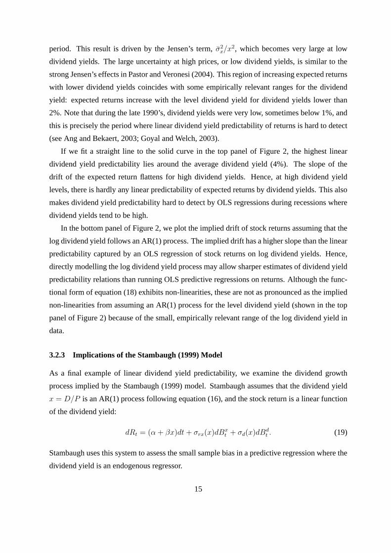
period. This result is driven by the Jensen’s term,σ2x/x

2, which becomes very large at low

dividend yields. The large uncertainty at high prices, or low dividend yields, is similar to the

strong Jensen’s effects in Pastor and Veronesi (2004). This region of increasing expected returns

with lower dividend yields coincides with some empirically relevant ranges for the dividend

yield: expected returns increase with the level dividend yield for dividend yields lower than

2%. Note that during the late 1990’s, dividend yields were very low, sometimes below 1%, and

this is precisely the period where linear dividend yield predictability of returns is hard to detect

(see Ang and Bekaert, 2003; Goyal and Welch, 2003).

If we fit a straight line to the solid curve in the top panel of Figure 2, the highest linear

dividend yield predictability lies around the average dividend yield (4%). The slope of the

drift of the expected return flattens for high dividend yields. Hence, at high dividend yield

levels, there is hardly any linear predictability of expected returns by dividend yields. This also

makes dividend yield predictability hard to detect by OLS regressions during recessions where

dividend yields tend to be high.

In the bottom panel of Figure 2, we plot the implied drift of stock returns assuming that the

log dividend yield follows an AR(1) process. The implied drift has a higher slope than the linear

predictability captured by an OLS regression of stock returns on log dividend yields. Hence,

directly modelling the log dividend yield process may allow sharper estimates of dividend yield

predictability relations than running OLS predictive regressions on returns. Although the func-

tional form of equation (18) exhibits non-linearities, these are not as pronounced as the implied

non-linearities from assuming an AR(1) process for the level dividend yield (shown in the top

panel of Figure 2) because of the small, empirically relevant range of the log dividend yield in

data.

3.2.3 Implications of the Stambaugh (1999) Model

As a final example of linear dividend yield predictability, we examine the dividend growth

process implied by the Stambaugh (1999) model. Stambaugh assumes that the dividend yield

x = D/P is an AR(1) process following equation (16), and the stock return is a linear function

of the dividend yield:

dRt = (α + βx)dt + σrx(x)dBxt + σd(x)dBd

t . (19)

Stambaugh uses this system to assess the small sample bias in a predictive regression where the

dividend yield is an endogenous regressor.

15

The Stambaugh model specifies two of the expected stock return, dividend yield, and stochas-

tic volatility. Proposition 2.1 implies that only one of these variables determines the other two,

once the dividend process is fixed. Hence, this system is over-parameterized if the dividends are

already specified. However, if we fix the expected stock return and the dividend yield, then this

implies that the dividend process must assume a very specific form. In particular, the dividend

yield can follow an AR(1) process and stock return predictability can be linear in the dividend

yield only if the dividend process itself is predicted by dividend yields. A further application of

Proposition 2.1 implies that the drift ofdDt/Dt in equation (2) can be written as a function of

the dividend yieldx:

α− κ +κθ

x− σ2

x

x2+ (β − 1)x. (20)

Hence, by assuming that dividend yields are mean-reverting, the linear dividend yield pre-

dictability of equation (19) implies that dividend yields must predict dividends.

We graph equation (20) in Figure 3, which shows that dividends are an increasing function

of dividend yields. This is consistent with the positive OLS predictive estimates reported by

Ang and Bekaert (2003) in the post-1952 Treasury Accord sample. This result is the opposite

implied by the intuition of Campbell and Shiller (1988a and b), who claim that high dividend

yields must forecast either high future returns, low future dividends, or both. According to

Campbell and Shiller’s reasoning, since high dividend yields should predict high returns from a

large, positiveβ coefficient in (19), high dividend yields should predict low future dividends, if

dividend yields predict dividends in the first place. This reasoning implies a downward sloping

drift of dividend growth as a function of dividend yields. In contrast, Figure 3 shows a non-

linear, but monotonically increasing drift of dividend growth as a function of dividend yields.

The incomplete reasoning of the Campbell and Shiller intuition is that it takes a static view

of the dividend yield being a function of returns and dividends. A high dividend yield today is

certainly caused by either high future returns, or low future dividend growth, or both. However,

there is an implicit assumption being made that the dividend yield also does not change in the

future. If dividend yields are mean-reverting, like in the Stambaugh model, then high dividend

yields today mean low dividend yields tomorrow. But, low dividend yields are associated with

either low returns or high dividend growth rates. The predictability equation (19) already im-

plies that today’s high dividend yield implies high expected returns. Thus, the only way that

dividend yields can be low next period with high expected returns is by increasing dividends

in the future. Thus, if dividend yields are mean-reverting and expected stock returns are posi-

tively linearly predicted by dividend yields, high dividend yields predict high, not low, dividend

16

growth rates.

3.3 Predictable Mean-Reverting Components of Returns

Mean-reversion of asset returns has been investigated by many authors, including Fama and

French (1988b) and Poterba and Summers (1986), and more recently in textbook treatments by

Campbell, Lo and MacKinlay (1997) and Cochrane (2001). Dividend yield predictability of

stock returns is a special case of a mean-reverting expected return. Our goal is to examine the

more general case of the expected stock return being a mean-reverting function of a predictable

state variable. With mean-reverting returns, Proposition 2.1 places strong restrictions on the

dynamics of prices and stock volatility. To characterize these restrictions, we work with IID

dividend growth, soµd = µd andσd = σd are constant in equation (2).

We assume that stock returns have a predictable componentxt:

dRt = xtdt + σrx(x)dBxt + σddBd

t , (21)

where the single mean-reverting state variablext follows an AR(1) process:

dxt = κ(θ − xt)dt + σxdBxt . (22)

Note thatθ is the unconditional mean of the continuously compounded stock return. The volatil-

ity σrx(x) is endogenously determined since we specify the conditional mean of the stock return.

From Proposition 2.1, the price-dividend ratioP/D = f(x) satisfies the following ordinary

differential equation:

−κ(θ − x)f ′ +1

2σ2

xf′′ −

(x− µd − 1

2σ2

d

)f = −1, (23)

which represents a perpetuity security in a Vasicek (1977) model with the short rate given by

x− µd − 12σ2

d. Oncef is determined,σrx = σx(ln f)′ is given by equation (10). Our goal is to

calibrate how much stochastic volatility of returns can be attributed to mean-reverting expected

returns. Since we assume dividend growth is IID, time-varying expected returns are also the

only source of heteroskedasticity.

Rather than solving equation (23), we can solve forf directly using expression (6) for the

price-dividend ratio. We can simplify equation (6) by writing:

Pt

Dt

= Et

[∫ ∞

t

exp

(−

∫ s

t

dxu

)exp

((µd +

1

2σd)s

)]

=

∫ ∞

t

exp

(−(θ − µd)s +

1

2σds

)Et

[exp

(−

∫ s

t

(xu − θ)du

)]ds.

17

It can be verified that the conditional expectation ofexp(− ∫ s

t(xu − θ)du

)is just the zero-

coupon bond price in a Vasicek (1977) model, with a short-rate process centered around zero,

and is given by:

Et

[exp

(−

∫ s

t

(xu − θ)du

)]

= exp

(−(xt − θ)

1− e−κs

κ+

σ2x

2κ2

(s− 2

1− e−κs

κ+

1− e−2κs

2κ

)).

Hence, we can write the price-dividend ratio as:9

Pt

Dt

=

∫ ∞

t

exp

(−(θ − µd)s +

1

2σds

−(xt − θ)1− e−κs

κ+

σ2x

2κ2

(s− 2

1− e−κs

κ+

1− e−2κs

2κ

))ds. (24)

Equation (24) is a strictly decreasing, concave function of the expected returnx. This im-

plies that the conditional expected return is a strictly increasing, convex function of the dividend

yield. We illustrate this in the top panel of Figure 4, which plots the expected returnx versus the

dividend yield using the valuesκ = 0.15, σx = 0.027, θ = 0.125, µd = 0.05, andσd = 0.07.

The value forθ is set from the average total continuously compounded return reported in Table

1. The values forκ andσx imply an annual autocorrelation of 0.86 and a volatility of 0.05 for

the conditional expected return. We expectκ to be low (or the persistence ofx to be high) be-

cause common instruments for predicting expected returns like dividend yields or interest rates

are persistent variables. Our values forκ and σx are in line with the implied autocorrelation

and volatilities for latent conditional expected returns reported by Brandt and Kang (2003), and

Johannes and Polson (2003), among others.

The bottom panel of Figure 4 reports the implied stochastic volatility parameterσrx(x) in

equation (21). The sign ofσrx is negative, implying a negative correlation between shocks

to expected returns and shocks to actual returns. Note that whileσrx is upward sloping, the

negative sign onσrx indicates that|σrx| is decreasing. This implies that heteroskedasticity

decreases as expected returns increase. This is counter-factual, as periods of high expected

returns (or market crashes) tend to coincide with periods of very high volatility. However, most

notable in the bottom panel of Figure 4 is that the magnitude ofσrx is extremely small, around

-0.0013. Hence, the total volatility of returns is effectively the same as the volatility of dividend

growth.

9 Equation (24) can be written as∫∞

texp(a(s) + b(s)xt)ds, which falls into the class of affine present value

models developed by Ang and Liu (2001), Bakshi and Chen (2002), and Bekaert and Grenadier (2002).

18

The intuition behind this result is that large changes inf (and consequentlyln f ) are re-

quired to produce a large amount of stochastic volatility through the relationσrx = σx(ln f)′ in

equation (10) of Proposition 2.1. When expected returns are mean-reverting, only the terms in

the sum (6) close tot change dramatically whenx changes. One way that large changes inf oc-

cur from changes inx is whenκ is close to zero, or expected returns are almost non-stationary.

This corresponds to the case of permanent changes in expected returns. Another alternative for

time-varying expected returns to re-produce the amount of stochastic volatility observed in data

is for the volatility of expected returns to be the same order of magnitude as the volatility of

returns. Since we observe low volatility of dividend growth, these results suggest that we may

need an additional volatility factor to explain the variability of returns.

3.4 Models of Stochastic Volatility

Variances of stock returns vary over time, and their dynamics have been successfully captured

by a number of models of stochastic volatility. If the dividend process is specified, Proposition

2.1 shows that the presence of stochastic volatility implies that stock returns must be predictable.

Since estimating variances is easier than estimating conditional means in small samples, as

Merton (1980) comments, we can use Proposition 2.1 to characterize stock return predictability

by parameterizing the variance process. Given recent econometric advances in inferring the

volatility process from an observed series of realized volatility (see Andersen et al., 2003),

Proposition 2.1 can be used to shed light on the nature of the aggregate risk-return relation, on

which there is no theoretical or empirical consensus.10 This is an entirely different approach

from the current approaches to estimating risk-return trade-offs, which use different measures of

conditional volatility in predictive regressions involving the conditional mean (see, for example,

Glosten, Jagannathan and Runkle, 1996).

We look at two well-known stochastic volatility models, the Gaussian model of Stein and

Stein (1991) in Section 3.4.1, and the square root model of Heston (1993) in Section 3.4.2.

In both cases, we assume that dividend growth is IID (µd = µd andσd = σd are constant in

equation (2)) to focus on the relations between risk and return.

10 For example, in two recent asset allocation applications involving stochastic volatility, Liu (2001) assumes

that the Sharpe ratio is increasing in volatility, following Merton (1973), while Chacko and Viceira (2000) assume

that the Sharpe ratio is a decreasing function of volatility.

19

3.4.1 The Stein-Stein (1991) Model

In the Stein and Stein (1991) model, the time-varying stock volatility is parameterized to be an

AR(1) process. The Stein-Stein model in our set-up can be written as:

dRt = µr(xt)dt + xtdBxt + σddBd

t

dxt = κ(θ − xt)dt + σxdBxt . (25)

The variance of the stock return isx2 + σ2d, so the stock return variance comprises a constant

componentσ2d, from dividend growth, and a mean-reverting componentx2. Empirically, shocks

to returns and shocks to volatility dynamics are strongly negatively correlated, which is termed

the leverage effect, soσx is negative.

The following corollary details the implicit restrictions are on the expected return of the

stockµr(·) by assuming that the stochastic volatility process follows the Stein-Stein model:

Corollary 3.4 Suppose that dividend growth is IID, soµd = µd andσd = σd are constant in

equation (2). If the stock variance is given byσrx(x) = x in equation (8), andx follows the

mean-reverting process (25) according to the Stein and Stein (1991) model, then the expected

stock returnµr(x) is given by:

µr(x) = µd +1

2σ2

d +1

2σx +

κθ

σx

x +

(1

2− κ

σx

)x2 + C−1 exp

(−1

2

x2

σx

), (26)

whereC is an integration constantC = f(0), wheref(0) is the price-dividend ratio at time

t = 0. Furthermore, we can describe the expected return in terms of the price-dividend ratio

f = P/D as:

µr(f) = µd +1

2σ2

d +1

2σx +

κθ

σx

√2∣∣∣σx ln

(f

C

) ∣∣∣ + (σx − 2κ) ln

(f

C

)+

1

f. (27)

The expected return (26) of the stock is a combination of several functional forms. First, the

expected return has a constant term, which is the case in a standard Lucas (1978) model with IID

consumption growth. Second, the expected return is proportional to volatilityx. This specifica-

tion is implied by models of first-order risk aversion, developed by Yaari (1987) and parameter-

ized by Epstein and Zin (1990). Third, the expected stock return is proportional to the variance

x2, which is the case in a Merton (1973) model. Finally, the last termC−1 exp(−12x2/σx) can

be shown to be the dividend yield in this economy. Since the price-dividend ratio is only one

component of equation (26), the Stein-Stein model predicts that expected returns may be non-

linear functions of price-dividend ratios or dividend yields. We emphasize that the risk-return

20

trade-off (26) is not derived using an equilibrium approach. The only economic assumptions

behind the risk-return trade-off is the IID dividend growth process and the no-bubble condition

necessary to derive Proposition 2.1.

We illustrate the risk-return relation (26) in the top panel of Figure 5. We graph the expected

return as a function of volatilityx using the parametersθ = 0.25, κ = 8 andσx = −0.2. These

parameter values are meant to be illustrative, and are consistent with stochastic volatility models

estimated by Chernov and Ghysels (2002), among others. These parameter values imply that

the unconditional standard deviation of volatility is 5%. We also chooseC = 24.5, which

represents the average price-dividend ratio in the data.

The risk-return trade-off in Figure 5 is highly non-linear. Expected returns initially decrease

as a function of volatility for low volatility values. For volatility values higher than 15%, the

expected stock return becomes a sharply increasing function of volatility. Empirically, the risk-

return relation is very hard to pin down. French, Schwert and Stambaugh (1987), Bollerslev,

Engle and Wooldridge (1988), Scruggs (1998) find only weak support for a positive risk-return

trade-off, while Ghysels, Santa-Clara and Valkanov (2003) find a significant and positive re-

lation. On the other hand, Campbell (1987) and Nelson (1991) find a significantly negative

relations. Glosten, Jagannathan and Runkle (1993), Scruggs (1998), and Harvey (2001) report

that the risk-return trade-off is negative, positive, or close to zero, depending on the specifica-

tion employed. The conflicting empirical findings of the risk-return trade-off are not surprising

in light of the decreasing and then increasing expected return as a function of volatility reported

in Figure 5. If the Stein and Stein (1991) volatility model is a reasonable description of the

data, Figure 5 suggests that an alternative appropriate risk-return empirical specification would

be a bi-linear form, so that the risk-return relation can take different slopes over low or high

volatilities.

To understand why the risk-return relation in the top panel of Figure 5 generally slopes up-

wards, consider the following intuition. The price-dividend ratiof in the Stein-Stein economy

is given byf = C−1 exp(−12x2/σx), which is a decreasing function of volatilityx becauseσx

is negative (due to the leverage effect).

If x is high (andf is low), because of mean-reversion,x is likely to be lowerf is likely to be

higher in the next period. The return is composed of a capital gain and a dividend component.

Since the dividend is IID, the higherf causes the capital gain component to be large for high

enough values ofx. Hence, high volatility levels correspond to high expected returns. The

opposite intuition occurs for low volatility levels. Whenx is low, andf is high, f is more

21

likely to be low in the next period because of mean-reversion, and the expected capital loss

causes expected returns to be low or negative for low volatility levels. The non-linearity of the

variance term in (26) is responsible for the non-monotonicity of the risk-return trade-off.

The bottom panel of Figure 5 plots the expected return as a function of the dividend yield

using equation (27). The expected return is an increasing function of the dividend yield. The

kink at the unconditional dividend yieldC−1 is due to the AR(1) formulation for the volatility

dynamics in equation (25), allowing volatility to go negative. This assumption is equivalent to

assuming a reflecting barrier atx = 0. An alternative model that restricts the volatility to be

positive and always smooth is the Heston (1993) model, which we examine next.

3.4.2 The Heston (1993) Model

In the Heston (1993) model, the variance follows a square-root process, similar to Cox, Ingersoll

and Ross (1987) that restricts the variance to be always positive. This modest change produces

a large change in the behavior of the risk premium, as the following corollary shows:

Corollary 3.5 Suppose that dividend growth is IID, soµd = µd andσd = σd are constant in

equation (2). Suppose that returns are described by the Heston (1993) model:

dRt = µr(xt)dt +√

xtdBxt + σddBd

t

dxt = κ(θ − xt)dt + σ√

xtdBxt (28)

Then, the expected stock returnµr(x) is given by:

µr(x) = µd +1

2σ2

d +κθ

σ+

(1

2− κ

σ

)x + C−1 exp

(−x

σ

), (29)

whereC is an integration constantC = f(0), wheref(0) is the price-dividend ratio at time

t = 0. Furthermore, we can describe the expected return in terms of the price-dividend ratio

f = P/D as:

µr(f) = µd +1

2σ2

d +κθ

σ+

(σ

2− κ

)ln

(f

C

)+

1

f. (30)

Like the Stein-Stein (1989) model,σ in equation (28) for the Heston (1993) model is neg-

ative empirically reflecting the leverage effect. We can interpret the risk-return trade-off in

equation (29) to have three components: a constant term, a term linear in the variancex, and the

third termf = C−1 exp(−x/σ) can be shown to be the dividend yield. Unlike the risk-return

trade-off in the Stein-Stein (1989) model (see equation (26)), there is no term proportional to

volatility√

x.

22

If C−1 is set to be the average dividend yield, which is approximately 4.4%, then the ex-

pected stock return in equation (29) is dominated by the linear term(12− κ

σ)x. Since empirical

estimates of the mean-reversion of the variance,κ, are large and estimates of the magnitude

of the volatility of the variance,σ, are small, the risk-return trade-off is upward sloping, for

empirically relevant parameters. Figure 6 illustrates this.

In the top panel of Figure 6, we plot the expected return (29) as a function of the stock

volatility√

x, to be comparable to the plots of the Stein-Stein (1991) model in Figure 5. We

choose the same calibrated parameters that Heston uses:θ = 0.01, κ = 2, andσ = −0.1. Fig-

ure 6 shows that the risk-return trade-off from a Heston model is always positive! Mechanically,

this is because the expected return in the Heston economy in equation (29) lacks a negative term

proportional to volatility that enters the risk-return trade-off in the Stein-Stein model (equation

(26)). The term proportional to volatility allows the expected return in the Stein-Stein solution

to initially decrease, before increasing. In the Heston model, no such initial decrease can oc-

cur. The bottom panel of Figure 6 shows that the expected return is an increasing function of

dividend yields, and looks remarkably similar to the corresponding picture for the Stein-Stein

model in Figure 5. The expected return as a function of the dividend yield is always smooth

because of the square-root process for variance in the Heston economy.

4 Conclusion

We derive conditions on expected returns, stock volatility, and price-dividend ratios that asset

pricing models must satisfy. In particular, given a dividend process, specifying only one of the

expected return process, the stochastic volatility process, or the price-dividend ratio process,

completely determines the other two processes. For example, the dividend stream allows the

volatility of stock returns to pin down the expected return. We do not need to specify a complete

equilibrium model to characterize these risk-return relations, but instead derive these conditions

using only the definition of returns, together with a transversality assumption.

Our conditions between risk and return are empirically relevant because many popular em-

pirical specifications assume dynamics for one, or a combination of, expected returns, volatility,

or price-dividend ratios, without considering the implicit restrictions on the dynamics of the

other variables. We show that some of these implied restrictions may result in strong, some-

times internally inconsistent, dynamics. Our results point the way to future empirical work that

can exploit our over-identifying conditions to create more powerful tests to investigate the risk-

23

return trade-off, the predictability of expected returns, the dynamics of stochastic volatility, and

present value relations in a unifying framework.

24

Appendix

A Proof of Proposition 2.1Equation (7) follows from a straightforward application of Ito’s lemma to the definition of the return:

dRt =dPt + Dtdt

Pt, (A-1)

which we rewrite asdRt = dft/ft + dDt/Dt + 1/ftdt. Note that we assume thatdBdt anddBx

t are uncorrelatedby assumption.

The definition of returns in equation (A-1) allows us to match the drift and diffusion terms in equation (7) forRt. Hence, the price-dividend ratiof , the expected returnµr, and the volatility termsσrx andσrd are determinedby re-arranging the drift, and thedBx

t and dBdt diffusion terms, respectively. If the expected returnµr(·) is

determined, equation (9) defines a differential equation forf , which determinesf . Oncef is determined, we cansolve forσrx from equation (10). If the return volatilityσrx is specified, we can solve forf from equation (10) upto a multiplicative constant, and this determines the expected returnµr in equation (9).¥

B Relation of Proposition 2.1 to Pricing Kernel FormulationsBy definition, given the dividend processDt, the price of the stock is given by:

Pt = Et

[∫ ∞

t

ΛsDs ds

], (B-1)

under the pricing kernel processΛt, together with a transversality assumption. We assume that the pricing kernelfollows:

dΛt

Λt= −rf (xt)dt− ξx(xt)dBx

t − ξd(xt)dBdt , (B-2)

whererf (·) is the risk-free rate process, andξx and ξd are prices of risk corresponding to shocks to the statevariablext and dividend growth, respectively. Using equation (B-1), we can express the price-dividend ratio as:

Pt

Dt= Et

[∫ ∞

t

exp(−

∫ s

t

(rf +12(ξ2

x + ξ2d)) du + ξx dBx

u + ξd dBdu

)

× exp(∫ s

t

µddu + σddBdu

)ds

].

This can be equivalently written as:

Pt

Dt= EQ

t

[∫ ∞

t

exp(−

∫ s

t

(rf − µd − 12(σd − ξd)2) du

)ds

], (B-3)

where the Radon-Nikodym derivative defining the risk-neutral measureQ is given by:

dQ

dP= exp

(−

∫ s

t

12(ξ2

x + (σd − ξd)2) du− ξx dBxu − (σd − ξd)dBd

u

). (B-4)

Note that equation (B-3) is a functionf of xt.We show how a particular choice of a return processdRt, together with assumptions on dividends, places

restrictions on the underlying pricing kernel processdΛt through the following proposition:

Proposition B.1 Suppose the state of the economy is described byxt, which follows equation (1), and a stock isa claim to the dividendsDt that are described by equation (2). If the stock return follows equation (7) and thepricing kernel process follows equation (B-2), then the price-dividend ratioPt/Dt = f(xt) satisfies the followingrelation:

(µx − ξxσx)f ′ +12σ2

xf ′′ − (rf − µd − 12σ2

d + ξdσd)f = −1, (B-5)

25

which determines the price-dividend ratiof . This implies that the expected returnµr(xt) and volatilityσrx(xt) ofthe return are given by:

µr = rf + ξxσx(ln f)′ + ξdσd,

σrx = σx(ln f)′ (B-6)

Proof: Equation (B-5) is the standard Feynman-Kac pricing equation. Once the price-dividend ratiof is obtainedfrom solving equation (B-5), we can derive equation (B-6) by equating terms from the drift term ofdRt and thediffusion term ondBx

t in equation (7).¥

Proposition B.1 states that, given the dividend stream, the pricing kernel completely determines the price-dividend ratiof , the expected return of the stockµr, and the volatility of the stockσrx. However, if we specifythe price of the stock, the expected return, or the volatility of the stock (each one being sufficient to determine theother two from Proposition 2.1), the short raterf , the prices of riskξx andξd, or the pricing kernelΛt are notuniquely determined. For example, suppose we specifyµr. There are potentially infinitely many pairs ofrf andξ = (ξx, ξd) that can produce the sameµr. For example, one (trivial) choice ofξ is ξ = (0, 0) corresponding torisk neutrality, and the stock return is the same as the risk-free rate. Whereas Proposition 2.1 shows that specifyingµr, σrx, orf completely determines the return process, the result from Proposition B.1 implies that a single choiceof µr, σrx, or f does not necessarily determine the pricing kernel.

C Proof of Corollary 3.1Statements (2) and (3) are equivalent from equation (10) of Proposition 2.1. Assume thatf = f is a constant.Then, using equation (9), we can show thatµr = f−1 + µd + 1

2 σ2d, which is a constant. Hence (2) follows from

(1). Finally, to show that (1) follows from (2), suppose thatµr = µr is a constant. From equation (9),f satisfiesthe following ODE:

µxf ′ +12σ2

xf ′′ −(

µr − µd − 12σ2

d

)f = −1. (C-1)

Since the term onf is constant, it follows that the price-dividend ratioP/D = f = (µr − µd − 12 σ2

d)−1 is thesolution. Note that this is just the Gordon formula, expressed in continuous-time. Hence, the price-dividend ratiois constant.¥

D Proof of Corollary 3.2Using equation (10) of Proposition 2.1, we haveσrx = σx(x)(ln f)′ = −1/x, sincef = 1/x. Rearranging, weobtain equationσx(x) = −σrxx. From equation (9), we have:

α + βx =µx(x)f ′ + 1

2 σ2rxx2f ′′ + 1

f+ µd +

12σ2

d. (D-1)

Substitutingf ′ = −1/x2 andf ′′ = 2/x3, and re-arranging this expression forµx(x) yields equation (14). Asimilar derivation is used for equation (15), except we employ the transformationx = − ln f , or f = e−x. ¥

E Proof of Corollary 3.3This is a straightforward application of equation (7) of Proposition 2.1, usingf = 1/x for the level dividend yieldandf = exp(−x) for the log dividend yield.¥

F Proof of Corollary 3.4Using equation (10) of Proposition 2.1, we have:x = σx(ln f)′, which we can solve for the price-dividend ratiofas:

f = C exp(

12

x2

σx

), (F-1)

26

whereC is the integration constantC = f(0). We can derive equation (26) by substituting the expression forf into equation (9) of Proposition 2.1. To derive equation (27), we use the expression forf to substitutex2 =2σx ln(f/C), andx =

√2|σx ln(f/C)|. ¥

G Proof of Corollary 3.5The proof is similar to Corollary 3.4, except now the price-dividend ratiof is given by:

f = C exp(x

σ

), (G-1)

whereC is the integration constantC = f(0). ¥

27

References[1] Ahn, D. H., R. F. Dittmar, and A. R. Gallant, 2002, “Quadratic Term Structure Models: Theory and Evi-

dence,”Review of Financial Studies, 15, 243-288.

[2] Andersen, T. G., T. Bollerslev, F. X. Diebold, and P. Labys, 2003, “Modeling and Forecasting RealizedVolatility,” Econometrica, 71, 529-626.

[3] Ang, A., 2002, “Characterizing the Ability of Dividend Yields to Predict Future Dividends in Log-LinearPresent Value Models,” working paper, Columbia Business School.

[4] Ang, A., and G. Bekaert, 2003, “Stock Return Predictability: Is It There?” working paper, Columbia BusinessSchool.

[5] Ang, A., and J. Liu, 2001, “A General Affine Earnings Valuation Model,”Review of Accounting Studies, 6,397-425.

[6] Bakshi, G., and Z. Chen, 2002, “Stock Valuation in Dynamic Economies,” working paper, University ofMaryland.

[7] Balduzzi, P., and A. W. Lynch, 1999, “Transaction Costs and Predictability: Some Utility Cost Calculations,”Journal of Financial Economics, 52, 47-78.

[8] Barberis, N., 2000, “Investing for the Long Run when Returns are Predictable,”Journal of Finance, 55, 1,225-264.

[9] Bekaert, G., and S. Grenadier, 2002, “Stock and Bond Pricing in an Affine Equilibrium,” working paper,Columbia Business School.

[10] Black, F., and M. S. Scholes, 1973, “The Pricing of Options and Corporate Liabilities,”Journal of PoliticalEconomy, 81, 637-659.

[11] Brandt, M., and Q. Kang, 2003, “On the Relationship Betweeen the Conditional Mean and Volatility of StockReturns: A Latent VAR Approach,” forthcomingJournal of Financial Economics.

[12] Bollerslev, T., R. F. Engle, and J. M. Wooldridge, 1988, “A Capital Asset Pricing Model with Time-VaryingCovariances,”Journal of Political Economy, 96, 116-131.

[13] Campbell, J. Y., 1993, “Intertemporal Asset Pricing without Consumption Data,”American Economic Re-view, 83, 487-512.

[14] Campbell, J. Y., 1987, “Stock Returns and the Term Structure,”Journal of Financial Economics, 18, 373-399.

[15] Campbell, J. Y., A. W. Lo, and A. C. MacKinlay, 1997,The Econometrics of Financial Markets, PrincetonUniversity Press, New Jersey.

[16] Campbell, J. Y., and R. J. Shiller, 1988a, “The Dividend-Price Ratio and Expectations of Future Dividendsand Discount Factors,”Review of Financial Studies, 1, 3, 195-228.

[17] Campbell, J. Y., and R. J. Shiller, 1988b, “Stock Prices, Earnings and Expected Dividends,”Journal ofFinance, 43, 3, 661-676.

[18] Campbell, J. Y., and L. M. Viceira, 1999, “Consumption and Portfolio Decisions when Expected Returns areTime Varying,”Quarterly Journal of Economics, 114, 433-495.

[19] Campbell, J. Y., and M. Yogo, 2003, “Efficient Tests of Stock Return Predictability,” working paper, HarvardUniversity.

[20] Chacko, G., and L. Viceira, 2000, “Dynamic Consumption and Portfolio Choice with Stochastic Volatility inIncomplete Markets,” working paper, Harvard University.

[21] Chernov, M., and E. Ghysels, 2002, “Towards a Unified Approach to the Joint Estimation of Objective andRisk Neutral Measures for the Purpose of Options Valuation,”Journal of Financial Economics, 56, 407-458.

[22] Cochrane, J. H., 2001,Asset Pricing, Princeton University Press, New Jersey.

[23] Constantinides, G. M., 1992, “A Theory of the Nominal Term Structure of Interest Rates,”Review of Finan-cial Studies, 5, 531-553.

[24] Cox, J. C., J. E. Ingersoll, Jr. and S. A. Ross, 1985, “A Theory Of The Term Structure Of Interest Rates,”Econometrica, 53, 2, 385-408.

28

[25] Engle, R. F., 1982, “Autoregressive Conditional Heteroscedasticity With Estimates Of The Variance OfUnited Kingdom Inflations,”Econometrica, 50, 4, 987-1008.

[26] Engstrom, E., 2003, “The Conditional Relationship between Stock Market Returns and the Dividend PriceRatio,” working paper, Columbia University.

[27] Epstein, L. G., and S. E. Zin, 1990, “ ‘First-Order’ Risk Aversion and the Equity Premium Puzzle,”Journalof Monetary Economics, 26, 387-407.

[28] Fama, E., and K. R. French, 1988a, “Dividend Yields and Expected Stock Returns,”Journal of FinancialEconomics, 22, 3-26.

[29] Fama, E., and K. R. French, 1988b, “Permanent and Temporary Components of Stock Prices,”Journal ofPolitical Economy, 96, 246-273.

[30] French, K. R., G. W. Schwert, and R. F. Stambaugh, 1987, “Expected Stock Returns and Volatility,”Journalof Financial Economics, 19, 3-29.

[31] Ferson, W., and C. R. Harvey, 1991, “The Variation of Economic Risk Premiums,”Journal of PoliticalEconomy, 99, 285-315.

[32] Ghysels, E., P. Santa-Clara, and R. Valkanov, 2003, “There is a Risk-Return Tradeoff After All,” workingpaper, UCLA.

[33] Glosten, L. R., R. Jagannathan, and D. E. Runkle, 1993, “On The Relation Between The Expected Value AndThe Volatility Of The Nominal Excess Return On Stocks,”Journal of Finance, 48, 5, 1779-1801.

[34] Goetzmann, W. N., and P. Jorion, 1993, “Testing the Predictive Power of Dividend Yields,”Journal of Fi-nance, 48, 2, 663-679.

[35] Goyal, A., and I. Welch, 2003, “The Myth of Predictability: Does the Dividend Yield Forecast the EquityPremium?”Management Science, 49, 5, 639-654.

[36] Grossman, S. J., and R. J. Shiller, 1981, “The Determinants of the Variability of Stock Market Prices,”American Economic Review, 71, 2, 222-227.

[37] Harvey, C. R., 1989, “Time-Varying Conditional Covariances in Tests of Asset Pricing Models,”Journal ofFinancial Economics, 24, 289-317.

[38] Harvey, C. R., 2001, “The Specification of Conditional Expectations,”Journal of Empirical Finance, 8,573-638.

[39] He, H., and H. Leland, 1993, “On Equilibrium Asset Price Processes,”Review of Financial Studies, 6, 3,593-617.

[40] Heston, S. L., 1993, “A Closed-Form Solution for Options with Stochastic Volatility with Applications toBond and Currency Options,”Review of Financial Studies, 6, 327-343.

[41] Hodrick, R. J., 1992, “Dividend Yields and Expected Stock Returns: Alternative Procedures for Inferenceand Measurement,”Review of Financial Studies, 5, 3, 357-386.

[42] Johannes, M., and N. Polson, 2003, “MCMC Methods for Continuous-Time Financial Econometrics,” work-ing paper, Columbia Business School.

[43] Kandel, S., and R. F. Stambaugh, 1996, “On the Predictability of Stock Returns: An Asset-Allocation Per-spective,”Journal of Finance, 51, 2, 385-424.

[44] Lamont, O., 1998, “Earnings and Expected Returns,”Journal of Finance, 53, 5, 1563-1587.

[45] Lettau, M., and S. Ludvigson, 2003, “Expected Returns and Expected Dividend Growth,” working paper,NYU.

[46] Lewellen, J., 2003, “Predicting Returns with Financial Ratios,” forthcomingJournal of Financial Economics.

[47] Liu, J., 2001, “Dynamic Portfolio Choice and Risk Aversion,” working paper, UCLA.

[48] Lo, A. W., and A. C. MacKinlay, 1988, “Stock Market Prices Do Not Follow Random Walks: Evidence FromA Simple Specification Test,”Review of Financial Studies, 1, 1, 41-66.

[49] Lucas, R. E., 1978, “Asset Prices in an Exchange Economy,”Econometrica, 46, 6, 1429-1445.

29

[50] Menzly, L., J. Santos, and P. Veronesi, 2004, “Understanding Predictability,”Journal of Political Economy,112, 1, 1-47.

[51] Merton, R. C., 1973, “An Intertemporal Capital Asset Pricing Model,”Econometrica, 41, 867-887.

[52] Merton, R. C., 1980, “On Estimating the Expected Return on the Market: An Exploratory Investigation,”Journal of Financial Economics, 8, 323-361.

[53] Nelson, D. B., 1991, “Conditional Heteroskedasticity in Asset Returns: A New Approach,”Econometrica,59, 347-370.

[54] Pastor, L., and P. Veronesi, 2004, “Was there a NASDAQ Bubble in the Late 1990’s?” working paper,University of Chicago.

[55] Poterba, J., and L. Summers, 1986, “The Persistence of Volatility and Stock Market Fluctuations,”AmericanEconomic Review, 76, 1142-1151.

[56] Richardson, M., 1993, “Temporary Components of Stock Prices: A Skeptic’s View,”Journal of Business andEconomic Statistics, 11, 2, 199-207.

[57] Scruggs, J. T., 1998, “Resolving The Puzzling Intertemporal Relation Between The Market Risk PremiumAnd Conditional Market Variance: A Two-Factor Approach,”Journal of Finance, 53, 2, 575-603.

[58] Shiller, R. J., 1981, “Do Stock Prices Move Too Much To Be Justified By Subsequent Changes In Divi-dends?,”American Economic Review, 71, 3, 421-436.

[59] Stambaugh, R. F., 1999, “Predictive Regressions,”Journal of Financial Economics, 54, 375-421.

[60] Stein, J. C., and E. Stein, 1991, ”Stock Price Distributions with Stochastic Volatility: An Analytic Approach”,Review of Financial Studies, 4, 727-752.

[61] Valkanov, R., 2003, “Long-Horizon Regressions: Theoretical Results and Applications,”Journal of FinancialEconomics, 68, 2, 201-232.

[62] Vasicek, O., 1977, “An Equilibrium Characterization Of The Term Structure,”Journal of Financial Eco-nomics, 5, 2, 177-188.

[63] Wachter, J., 2002, “Portfolio Consumption Decisions under Mean-Reverting Returns: An Exact Solution forComplete Markets,”Journal of Financial and Quantitative Analysis, 1, 63-91.

[64] Yaari, M. E., 1987, “The Dual Theory of Choice under Risk,”Econometrica, 55, 95-115.

30

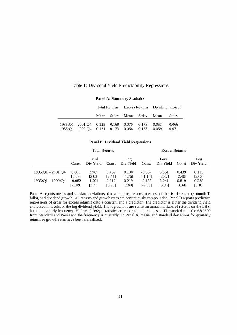
Table 1: Dividend Yield Predictability Regressions

Panel A: Summary Statistics

Total Returns Excess Returns Dividend Growth

Mean Stdev Mean Stdev Mean Stdev

1935:Q1 – 2001:Q4 0.125 0.169 0.070 0.173 0.053 0.0661935:Q1 – 1990:Q4 0.121 0.173 0.066 0.178 0.059 0.071

Panel B: Dividend Yield Regressions

Total Returns Excess Returns

Level Log Level LogConst Div Yield Const Div Yield Const Div Yield Const Div Yield

1935:Q1 – 2001:Q4 0.005 2.967 0.452 0.100 -0.067 3.351 0.439 0.113[0.07] [2.03] [2.41] [1.76] [-1.10] [2.37] [2.40] [2.03]

1935:Q1 – 1990:Q4 -0.082 4.591 0.812 0.219 -0.157 5.041 0.819 0.238[-1.09] [2.71] [3.25] [2.80] [-2.08] [3.06] [3.34] [3.10]

Panel A reports means and standard deviations of total returns, returns in excess of the risk-free rate (3-month T-bills), and dividend growth. All returns and growth rates are continuously compounded. Panel B reports predictiveregressions of gross (or excess returns) onto a constant and a predictor. The predictor is either the dividend yieldexpressed in levels, or the log dividend yield. The regressions are run at an annual horizon of returns on the LHS,but at a quarterly frequency. Hodrick (1992) t-statistics are reported in parentheses. The stock data is the S&P500from Standard and Poors and the frequency is quarterly. In Panel A, means and standard deviations for quarterlyreturns or growth rates have been annualized.

31

Figure 1: Implied Drift of the Level or Log Dividend Yield

0 0.02 0.04 0.06 0.08 0.1 0.12 0.14−0.05

−0.04

−0.03

−0.02

−0.01

0

0.01Implied Drift of the Level Dividend Yield

Dividend Yield (Level)

Drif

tImplied DriftLinear Approximation from Data

−3.6 −3.4 −3.2 −3 −2.8 −2.6 −2.4 −2.2 −2

−0.3

−0.25

−0.2

−0.15

−0.1

−0.05

0

0.05

0.1

0.15Implied Drift of the Log Dividend Yield

Log Dividend Yield

Drif

t

Implied DriftLinear Approximation from Data

In the top panel, we graph the implied drift of the level dividend yield (equation (14)) using the calibrated parametervaluesµd = 0.05, σd = 0.07, σrd = 0.15, α = −0.08, andβ = 4.6 in the solid line. The dotted line representsthe drift of an AR(1) fitted to the level dividend yield in dataκ(θ − x), where0.96 = exp(−κ/4) andθ = 0.044in equation (16). In the bottom panel, we plot the implied drift of the log dividend yield (equation (15)) usingα = 0.81 andβ = 0.22. The approximating AR(1) drift is produced by using0.94 = exp(−κ/4) andθ = −3.16in equation (16). The calibrations are done using quarterly S&P500 data from 1935 to 1990.

32

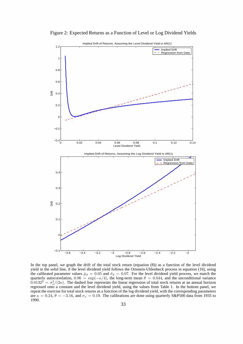
Figure 2: Expected Returns as a Function of Level or Log Dividend Yields

0 0.02 0.04 0.06 0.08 0.1 0.12 0.14−0.4

−0.2

0

0.2

0.4

0.6

0.8

1

1.2Implied Drift of Returns, Assuming the Level Dividend Yield is AR(1)

Level Dividend Yield

Drif

tImplied DriftRegression from Data

−3.6 −3.4 −3.2 −3 −2.8 −2.6 −2.4 −2.2 −2−0.1

0

0.1

0.2

0.3

0.4

Implied Drift of Returns, Assuming the Log Dividend Yield is AR(1)

Log Dividend Yield

Drif

t

Implied DriftRegression from Data

In the top panel, we graph the drift of the total stock return (equation (8)) as a function of the level dividendyield in the solid line, if the level dividend yield follows the Ornstein-Uhlenbeck process in equation (16), usingthe calibrated parameter valuesµd = 0.05 and σd = 0.07. For the level dividend yield process, we match thequarterly autocorrelation,0.96 = exp(−κ/4), the long-term meanθ = 0.044, and the unconditional variance0.01322 = σ2

x/(2κ). The dashed line represents the linear regression of total stock returns at an annual horizonregressed onto a constant and the level dividend yield, using the values from Table 1. In the bottom panel, werepeat the exercise for total stock returns as a function of the log dividend yield, with the corresponding parametersareκ = 0.24, θ = −3.16, andσx = 0.19. The calibrations are done using quarterly S&P500 data from 1935 to1990.

33

Figure 3: Drift of Dividend Growth Implied by the Stambaugh (1999) System

0 0.02 0.04 0.06 0.08 0.1 0.12 0.14−1.2

−1

−0.8

−0.6

−0.4

−0.2

0

0.2

0.4

Level Dividend Yield

Drif

t

We graph the drift of dividend growthdDt/Dt (equation (20)) from the Stambaugh (1999) system, where the leveldividend yieldx is mean-reverting in equation (16), and stock returns are linearly predicted by dividend yields inequation (19). We use the parameter valuesκ = 0.16, θ = 0.044, σx = 0.0075, α = −0.08 andβ = 4.60. Thecalibrations are done using quarterly S&P500 data from 1935 to 1990.

34

Figure 4: Implications for Predictability and Stochastic Volatility from Mean-Reverting Ex-pected Returns

0.03 0.04 0.05 0.06 0.07 0.08 0.090

0.02

0.04

0.06

0.08

0.1

0.12

0.14

0.16

0.18

0.2Expected Return versus Dividend Yield

Dividend Yield

Exp

ecte

d R

etur

n

0 0.02 0.04 0.06 0.08 0.1 0.12 0.14 0.16 0.18 0.2−1.4

−1.35

−1.3

−1.25

−1.2

−1.15x 10

−3 Stochastic Volatility σrx

Vol

atili

ty o

f Ret

urns

Expected Return

In the top panel, we graph the conditional expected returnx versus the dividend yield, obtained from invertingequation (24), using the parameter valuesκ = 0.15, σx = 0.027, θ = 0.125, µd = 0.05, andσd = 0.07. In thebottom panel, we graph the implied stochastic volatility parameterσrx(·) in equation (21) as a function ofx. Toproduce the plots, we use quadrature to solve the price-dividend ratio in equation (24), and then numerically takederivatives of the log price-dividend ratio to computeσrx(·).

35

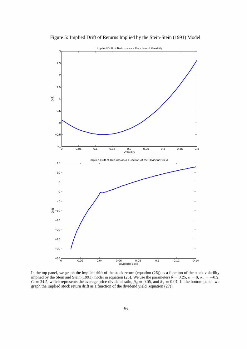
Figure 5: Implied Drift of Returns Implied by the Stein-Stein (1991) Model

0 0.05 0.1 0.15 0.2 0.25 0.3 0.35 0.4−1

−0.5

0

0.5

1

1.5

2

2.5

3

Volatility

Drif

tImplied Drift of Returns as a Function of Volatility

0 0.02 0.04 0.06 0.08 0.1 0.12 0.14−35

−30

−25

−20

−15

−10

−5

0

5

10

15

Dividend Yield

Drif

t

Implied Drift of Returns as a Function of the Dividend Yield

In the top panel, we graph the implied drift of the stock return (equation (26)) as a function of the stock volatilityimplied by the Stein and Stein (1991) model in equation (25). We use the parametersθ = 0.25, κ = 8, σx = −0.2,C = 24.5, which represents the average price-dividend ratio,µd = 0.05, andσd = 0.07. In the bottom panel, wegraph the implied stock return drift as a function of the dividend yield (equation (27)).

36

Figure 6: Implied Drift of Returns Implied by the Heston (1993) Model

0 0.05 0.1 0.15 0.2 0.25 0.3 0.35 0.4−0.5

0

0.5

1

1.5

2

2.5

3

3.5

Volatility

Drif

t

Implied Drift of Returns as a Function of Volatility

0 0.02 0.04 0.06 0.08 0.1 0.12 0.14−4

−3

−2

−1

0

1

2

3

Dividend Yield

Drif

t

Implied Drift of Returns as a Function of the Dividend Yield

In the top panel, we graph the implied drift of the stock return (equation (29)) as a function of the stock volatilityimplied by the Stein and Stein (1991) model in equation (28). We use the parametersθ = 0.01, κ = 2, σ = −0.1,which are the parameters used by Heston (1993),C = 24.5, which represents the average price-dividend ratio,µd = 0.05, and σd = 0.07. In the bottom panel, we graph the implied stock return drift as a function of thedividend yield (equation (30)).

37