Risk Theory Calculations Using R and

actuar

Vincent Goulet, Ph.D.

École d’actuariat, Université Laval

Québec, Canada

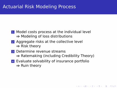
Actuarial Risk Modeling Process

1 Model costs process at the individual level

⇒ Modeling of loss distributions

2 Aggregate risks at the collective level

⇒ Risk theory

3 Determine revenue streams

⇒ Ratemaking (including Credibility Theory)

4 Evaluate solvability of insurance portfolio

⇒ Ruin theory

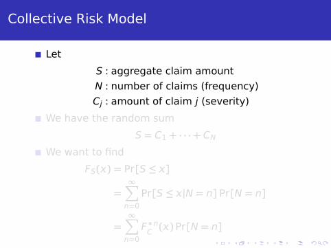
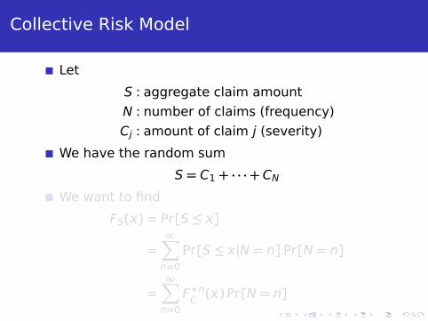
Collective Risk Model

Let

S : aggregate claim amount

N : number of claims (frequency)

Cj : amount of claim j (severity)

We have the random sum

S = C1 + · · ·+ CNWe want to find

FS() = Pr[S ≤ ]

=∞∑

n=0Pr[S ≤ |N = n]Pr[N = n]

=∞∑

n=0F∗nC ()Pr[N = n]

Collective Risk Model

Let

S : aggregate claim amount

N : number of claims (frequency)

Cj : amount of claim j (severity)

We have the random sum

S = C1 + · · ·+ CNWe want to find

FS() = Pr[S ≤ ]

=∞∑

n=0Pr[S ≤ |N = n]Pr[N = n]

=∞∑

n=0F∗nC ()Pr[N = n]

Collective Risk Model

Let

S : aggregate claim amount

N : number of claims (frequency)

Cj : amount of claim j (severity)

We have the random sum

S = C1 + · · ·+ CNWe want to find

FS() = Pr[S ≤ ]

=∞∑

n=0Pr[S ≤ |N = n]Pr[N = n]

=∞∑

n=0F∗nC ()Pr[N = n]

Aggregate Claim Amount Distribution

Function aggregateDist() supports five methods

Main one is the recursive method (Panjer

algorithm):

fS() =1

1− fC(0)

�

(p1 − (+ b)p0)fC()

+min(,m)∑

y=1(+ by/)fC(y)fS(− y)

�

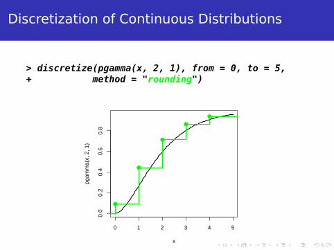
Discretization of Continuous Distributions

> discretize(pgamma(x, 2, 1), from = 0, to = 5,+ method = "upper")

0 1 2 3 4 5

0.0

0.2

0.4

0.6

0.8

x

pgam

ma(

x, 2

, 1)

●

●

●

●

●

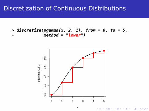
Discretization of Continuous Distributions

> discretize(pgamma(x, 2, 1), from = 0, to = 5,+ method = "lower")

0 1 2 3 4 5

0.0

0.2

0.4

0.6

0.8

x

pgam

ma(

x, 2

, 1)

●

●

●

●

●

●

Discretization of Continuous Distributions

> discretize(pgamma(x, 2, 1), from = 0, to = 5,+ method = "rounding")

0 1 2 3 4 5

0.0

0.2

0.4

0.6

0.8

x

pgam

ma(

x, 2

, 1)

●

●

●

●

●

Discretization of Continuous Distributions

> discretize(pgamma(x, 2, 1), from = 0, to = 5,+ method = "unbiased",+ lev = levgamma(x, 2, 1))

0 1 2 3 4 5

0.0

0.2

0.4

0.6

0.8

x

pgam

ma(

x, 2

, 1)

●

●

●

●

●●

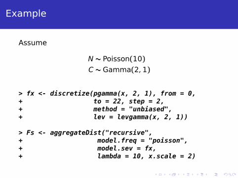
Example

Assume

N ∼ Poisson(10)C ∼ Gamma(2,1)

> fx <- discretize(pgamma(x, 2, 1), from = 0,+ to = 22, step = 2,+ method = "unbiased",+ lev = levgamma(x, 2, 1))

> Fs <- aggregateDist("recursive",+ model.freq = "poisson",+ model.sev = fx,+ lambda = 10, x.scale = 2)

Example (continued)

> plot(Fs)

0 10 20 30 40 50 60

0.0

0.2

0.4

0.6

0.8

1.0

Aggregate Claim Amount Distribution

x

FS((x

))

Recursive method approximation

Example (continued)

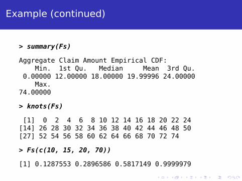
> summary(Fs)

Aggregate Claim Amount Empirical CDF:Min. 1st Qu. Median Mean 3rd Qu.

0.00000 12.00000 18.00000 19.99996 24.00000Max.

74.00000

> knots(Fs)

[1] 0 2 4 6 8 10 12 14 16 18 20 22 24[14] 26 28 30 32 34 36 38 40 42 44 46 48 50[27] 52 54 56 58 60 62 64 66 68 70 72 74

> Fs(c(10, 15, 20, 70))

[1] 0.1287553 0.2896586 0.5817149 0.9999979

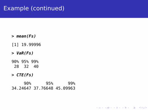
Example (continued)

> mean(Fs)

[1] 19.99996

> VaR(Fs)

90% 95% 99%28 32 40

> CTE(Fs)

90% 95% 99%34.24647 37.76648 45.09963

Long Term Risk Analysis

Study evolution of the surplus of the insurance

company over many periods of time

Quantity of interest: probability that surplus

becomes negative

Technical ruin of the insurance company ensues

Equivalent idea in other fields

Continuous Time Ruin Model

Let

U(t) : surplus at time tc(t) : premiums collected through time tS(t) : aggregate claims paid through time t

If is the initial surplus at time t = 0, then we have

U(t) = + c(t)− S(t)

We want

ψ() = Pr[U(t) < 0 for some t ≥ 0]

Continuous Time Ruin Model

Let

U(t) : surplus at time tc(t) : premiums collected through time tS(t) : aggregate claims paid through time t

If is the initial surplus at time t = 0, then we have

U(t) = + c(t)− S(t)

We want

ψ() = Pr[U(t) < 0 for some t ≥ 0]

Continuous Time Ruin Model

Let

U(t) : surplus at time tc(t) : premiums collected through time tS(t) : aggregate claims paid through time t

If is the initial surplus at time t = 0, then we have

U(t) = + c(t)− S(t)

We want

ψ() = Pr[U(t) < 0 for some t ≥ 0]

Ruin Probabilities

If Wj ∼ Exponential(λ) and Cj ∼ Exponential(β), then

ψ() =λ

cβe−(β−λ/c)

Most common distributions for claim amounts and

waiting times:

mixtures of exponentials

mixtures of Erlang

phase-type

In most cases ruin() computes probabilities with

pphtype()

Example

Mixture of two exponentials for claims, exponential

interarrival times

> psi <- ruin(claims = "exponential",+ par.claims = list(rate = c(3, 7),+ weights = 0.5),+ wait = "exponential",+ par.wait = list(rate = 3),+ premium.rate = 1)

> u <- 0:10> psi(u)

[1] 7.142857e-01 2.523310e-01 9.280151e-02[4] 3.413970e-02 1.255930e-02 4.620307e-03[7] 1.699716e-03 6.252905e-04 2.300315e-04

[10] 8.462387e-05 3.113138e-05

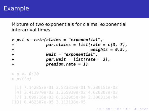
Example

Mixture of two exponentials for claims, exponential

interarrival times

> psi <- ruin(claims = "exponential",+ par.claims = list(rate = c(3, 7),+ weights = 0.5),+ wait = "exponential",+ par.wait = list(rate = 3),+ premium.rate = 1)

> u <- 0:10> psi(u)

[1] 7.142857e-01 2.523310e-01 9.280151e-02[4] 3.413970e-02 1.255930e-02 4.620307e-03[7] 1.699716e-03 6.252905e-04 2.300315e-04

[10] 8.462387e-05 3.113138e-05

Example (continued)

> plot(psi, from = 0, to = 10)

0 2 4 6 8 10

0.0

0.1

0.2

0.3

0.4

0.5

0.6

0.7

Probability of Ruin

u

ψψ((u

))

Simulation of Compound Hierarchical Models

You want to simulate data from this model?

Xjt |Λj,Θ ∼ Poisson(Λj), t = 1, . . . , njΛj|Θ ∼ Gamma(3,Θ), j = 1, . . . , JΘ ∼ Gamma(2,2), = 1, . . . , ,

●

ΘΘi

ΛΛi j

Xi j t

i = 1, ..., I

j = 1, ..., J i

t = 1, ..., ni j

● ● ●

ΘΘi

ΛΛi j|ΘΘi

Xi j t|ΛΛi j,

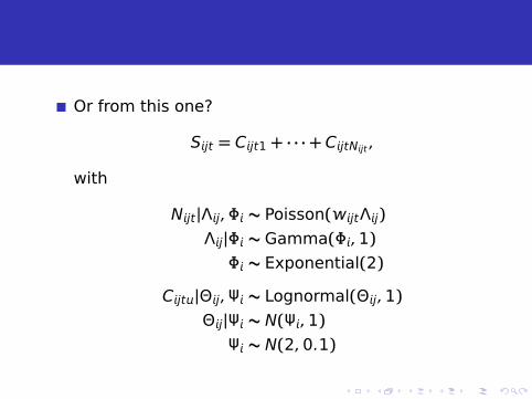
Or from this one?

Sjt = Cjt1 + · · ·+ CjtNjt ,

with

Njt |Λj, ∼ Poisson(jtΛj)Λj| ∼ Gamma(,1) ∼ Exponential(2)

Cjt|Θj,Ψ ∼ Lognormal(Θj,1)Θj|Ψ ∼ N(Ψ,1)

Ψ ∼ N(2,0.1)

Using only R syntax (i.e. without reverting to

BUGS)?

Then read this fine paper:

Goulet, V., Pouliot, L.-P. (2008), Simulation ofCompound Hierarchical Models in R, North

American Actuarial Journal, 12, 401–412.

More Information

Project’s web site

http://www.actuar-project.org

Package vignettes

actuar Introduction to actuarcoverage Complete formulas used by

coveragecredibility Risk theory featureslossdist Loss distributions modeling

featuresrisk Risk theory features

Demo files