Risk, Uncertainty, and Option Exercise∗

Jianjun Miao† and Neng Wang‡

January 7, 2004

Abstract

Many economic decisions can be described by an option exercise problem. Thestandard real options approach emphasizes the importance of uncertainty indetermining option value and timing of option exercise. No distinction betweenrisk and uncertainty is made. Motivated by the experimental evidence suchas the Ellsberg Paradox, we follow Knight (1921) and distinguish risk fromuncertainty. To afford this distinction, we adopt the multiple-priors utilitymodel to analyze an option exercise problem. We also provide several examplesto illustrate that our model can explain some phenomena that are hard toreconcile with the standard real options model. These examples include realinvestment, job search, firm exit, firm default, and youth suicide.

JEL Classification: D81

Keywords: Knightian uncertainty, multiple-priors utility, real options, optimalstopping problem

∗We thank .†Department of Economics, Boston University, Boston, MA 02215. Email: miaoj@bu.edu. Tel.:

617-353-6675.‡William E. Simon School of Business Administration, University of Rochester, Rochester, NY

14627. Email: wang@simon.rochester.edu; Tel.: 585-275-4896.

1 Introduction

Many economic decisions can be described by binary choices. Examples are abundant.

A firm may decide whether or not to invest in a project. It may also decide whether

or not to exit an industry. If a corporate firm takes on debt, it has to decide whether

or not to default. A worker may decide whether or not to accept a job offer. A dismal

person may decide whether or not to commit suicide.

All these decisions share three characteristics. First, the decision is irreversible.

Second, there is uncertainty about future rewards. Third, agents have some leeway

about the timing of decisions. These three characteristics imply that waiting has

positive value. In other words, all the above problems can be viewed as a problem

where agents decide when to exercise an “option” analogous to a financial call option

– it has the right but not the obligation to buy an asset at some future time of its

choosing. This real options approach has been widely applied in investments and

corporate finance (see Dixit and Pindyck (1994)).

As argued by Dixit (1992), the standard real options approach to investment under

uncertainty can be summarized as “a theory of optimal inertia”. “It says that firms

that refuse to invest even when the currently available rates of return are far in excess

of the cost of capital may be optimally waiting to be surer that this state of affairs

is not transitory. Likewise, farmers who carry large losses may be rationally keeping

their operation alive on the chance that the future may be brighter” (Dixit (1992,

p.109)).

However, the standard real options approach rules out the situation where agents

are unsure about the likelihoods of future events. It typically adopts strong as-

sumptions about agents’ beliefs. For example, according to the rational expectations

hypothesis, agents know precisely the objective probability law of the state process

and their beliefs are identical to this probability law. Alternatively, according to

the Bayesian approach, an agent’s beliefs are represented by a subjective probability

1

measure or Bayesian prior. There is no meaningful distinction between risk, where

probabilities are available to guide choice, and uncertainty, where information is too

imprecise to be summarized adequately by probabilities. By contrast, Knight (1921)

emphasizes this distinction and argues that uncertainty is more common in decision-

making.1 For experimental evidence, the Ellsberg Paradox suggests that people prefer

to act on known rather than unknown or ambiguous probabilities.2 Ellsberg-type be-

havior contradicts the Bayesian paradigm, i.e., the existence of any prior underlying

choices.

To incorporate Knightian uncertainty or ambiguity, we adopt the multiple-priors

utility model (Gilboa and Schmeidler (1989), Epstein and Wang (1994)). This model

is axiomatized by Gilboa and Schmeidler (1989) in a static setting and by Epstein and

Schneider (2002) in a dynamic setting. In this model, the agent beliefs are represented

by a set of priors. The set of priors captures both the degree of Knightian uncertainty

and uncertainty aversion.3

We first describe an agent’s option exercise decision as an optimal stopping prob-

lem. We then characterize the solution under Knightian uncertainty and compare

it to that in the standard model. We find that the option value under Knightian

uncertainty is smaller than that in the standard model. Moreover, an uncertainty

averse agent exercises the option earlier than an expected utility maximizer.

The standard real options approach emphasizes the importance of uncertainty in

determining option value and timing of option exercise. Implicitly assumed, uncer-

tainty is identical to risk. Recognizing the difference between risk and uncertainty,

we conduct comparative statics with respect to the set of priors. We find that if an

1Henceforth, we refer to such uncertainty as Knightian uncertainty or ambiguity.2See Ellsberg (1961). One version of the story is as follows. A decision maker is a offerred a

bet on drawing a red ball from two urns. The first urn contains exactly 50 red and 50 black balls.

The second urn has 100 balls, either red or black, however the exact number of red or black balls is

unknown. Vast majority agents choose from the first urn rather than the second.3For a formal definition of uncertainty aversion, see Epstein (1999) and Epstein and Zhang (2001).

2

agent is more uncertainty averse or faces a higher level of Knightian uncertainty, then

the option value is lower and the agent exercises the option earlier.

We provide several examples to apply our results, including real investment, job

search, firm exit, firm default, and youth suicide. These examples illustrate that

our model can explain some phenomena that may be hard to be reconciled with the

standard real options model.

The multiple-priors utility model has been applied to asset pricing and portfolio

choice problems in a number of papers.4 To our knowledge, our paper is the first to

apply the multiple-priors utility model to study real options problems.

A related approach based on robust control theory is proposed by Hansen and

Sargent and their coauthors.5 They emphasize ‘model uncertainty’ which is also

motivated in part by the Ellsberg Paradox . We refer readers to Epstein and Schneider

(2002) for further discussion on these two approaches.

The paper is organized as follows. Section 2 presents the model and states as-

sumptions. Section 3 provides and analyzes main results. Section 4 presents several

applications. Section 5 concludes.

2 The Model

2.1 Background

Before presenting the model, we first provide some background about multiple-priors

utility. The static multiple-priors utility model of Gilboa and Schmeidler (1989) can

be described informally as follows. Suppose uncertainty is represented by a measur-

able space (S,F) . The decision-maker ranks uncertain prospects or acts, maps from

S into an outcome set X . Then the multiple-priors utility U (f) of any act f has the

4See Epstein and Wang (1994, 1995), Chen and Epstein (2001), Epstein and Miao (2003), Kogan

and Wang (2002), Cao et al (2002), and Routledge and Zin (2003).5See, for example, Anderson, Hansen and Sargent (2003) and Hansen and Sargent (2000).

3

functional form:

U (f) = minQ∈∆

∫

u (f) dQ,

where u : X → R is a von Neumann-Morgenstern utility index and ∆ is a subjective

set of probability measures on (S,F) . Intuitively, the multiplicity of priors models

ambiguity about likelihoods of events and the minimum delivers aversion to such

ambiguity. The standard expected utility model is obtained when the set of priors ∆

is a singleton.

The Gilboa and Schmeidler model is generalized to a dynamic setting in discrete

time by Epstein and Wang (1994). Their model can be described briefly as follows.

The time t conditional utility from a consumption process c = (ct)t≥0 is defined by

the recursion

Vt (c) = u (ct) + β minQ∈P

EQt [Vt+1 (c)] , (1)

where β ∈ (0, 1) is the discount factor, EQt is the conditional expectation operator

with respect to measure Q, and P is a set of one-step-ahead conditional probability

measures. An important feature of this utility is that it satisfies dynamic consistency

because of the recursivity of utility (1).6 This model will be adopted below.

2.2 Example

To understand our model and results, an illustrative example proves useful. Consider

an investor who contemplates to invest irreversibly in a project in a three period

setting. Assume that the investor is risk neutral and discounts cash flows by β = 0.2.

The payoff in period 0 is certain, while the payoffs in periods 1 and 2 are uncertain.

Investment costs I = 145. The initial value of the project is x = 100. In periods

1 and 2, the value of the project may go up or down by 50% (see Figure 1). These

events are independent.

6See Epstein and Schneidler (2002) for further discussion on this model and dynamic consistency.

4

x

PP

PP

1.5x

0.5x

PP

PP

PP

PP

2.25x

0.75x

0.25x

Figure 1: Investment cash flows

In standard models, the investor views the investment as purely risky. We may

suppose that up and down have equal probability. Then according to the Marshallian

net present value principle, the investor will not invest at period zero since the net

present value of the investment opportunity is

NPV = x + β (1.5x + 0.5x) /2 + β2 (2.25x/4 + 0.75x/2 + 0.25x/4) − I = −21 < 0.

However, if the investor can postpone the investment, he can observe whether the

value of the project goes up or not. He can avoid the downside loss by investing when

the value goes up. We use backward induction to solve the problem. It is clear that

the value of the investment at period 2, F2, is positive only when the project value is

2.25x,

F2 (2.25x) = max2.25x − I, 0 = 80.

Next, one can show that the value of the investment at period 1, F1, is positive only

for the project value 1.5x,

F1 (1.5x) = max 1.5x − I, 0.5βF2 (2.25x) = 8 > 1.5x − I.

Finally, the value of the investment in period 0 is

F0 (x) = max x − I, 0.5βF1 (1.5x) = 0.8 > 0 > x − I.

5

Thus, the investor will wait to invest at period 2 if and only if the value of the project

goes up in both periods 1 and 2. This example illustrates the key idea of the real

options approach that waiting has positive value.

Now, consider the situation under which the investor is ambiguous about the

project value. Suppose he thinks that the value of the project goes up with probability

1/2 or 1/4. He is risk neutral and his preferences are represented by (1). We still use

backward induction. Again, in period 2, the investment has positive value only for

the project value 2.25x,

V2 (2.25x) = max2.25x − I, 0 = 80.

In period 1, the investor compares the value of immediate investment with that if

waiting until period 2. However, the investor values period 2 investment by taking

the worst scenario. It can be shown that the value of the investment is positive only

when the project value is 1.5x,

V1 (1.5x) = max

1.5x − I, β1

4V2 (2.25x)

= 5 > β1

4V2 (2.25x) .

Finally, by a similar calculation, the period zero value of the investment is

V0 (x) = max

x − I, β1

4V1 (1.5x)

= 0.25 > x − I.

The above two inequalities state that an uncertainty averse investor chooses optimally

to invest in period 1, when the project value goes up. Moreover, he has a lower option

value than the investor with expected utility since V0 (x) < F0 (x) .

In summary, this example shows that waiting has positive value for both uncer-

tainty averse agent and the expected utility maximizer. However, the option value of

the investment opportunity is lower under Knightian uncertainty than in the standard

model. Therefore, an uncertainty averse agent invests earlier. We next turn to the

formal model.

6

2.3 Setup

Consider an infinite horizon discrete time optimal stopping problem. As explained

in Dixit and Pindyck (1994), the optimal stopping problem can be applied to study

an agent’s option exercise decision. The agent’s choice is binary. In each period, he

decides on whether stopping a process and taking a termination payoff, or continuing

for one period, and making the same decision in the future.

Formally, uncertainty is generated by a Markov state process (xt)t≥0 taking values

in X ⊂ R. The probability kernel of (xt)t≥0 is given by P : X → M (X) , where

M (X) is the space of probability measures on X endowed with the weak convergence

topology. Continuation at date t generates a payoff π (xt) , while stopping at date t

yields a payoff Ω (xt) , where π and Ω are functions that map X into R. Suppose the

agent is risk neutral and discount future payoff flows by β ∈ (0, 1).

In standard models, the agent’s preferences are represented by time-additive ex-

pected utility. As in the rational expectations paradigm, P can be interpreted as

the objective probability law governing the state process (xt)t≥0, and is known to the

agent. The expectation in the utility function is taken with respect to this law. Al-

ternatively, according to the Savage utility representation theorem, P is a subjective

(one-step-ahead) prior and represents the agent’s beliefs. By either approach, the

standard stopping problem can be described by the following dynamic programming

problem:

F (x) = max

Ω (x) , π (x) + β

∫

F (x′) P (dx′; x)

, (2)

where the value function F can be interpreted as an option value.

To fix ideas, we make the following assumptions. These assumptions are standard

in dynamic programming theory (see Stokey and Lucas (1989)).

Assumption 1 π : X → R is bounded, continuous, and increasing.

Assumption 2 Ω : X → R is bounded, continuous and increasing.

7

Assumption 3 P is increasing and satisfies the Feller property. That is,∫

f (x′) P (dx′; x)

is increasing in x for any increasing function f and is continuous in x for any bounded

and continuous function f.

The following proposition describes the solution to problem (2).

Proposition 1 Let Assumptions 1-3 hold. Then there exists a unique bounded, con-

tinuous and increasing function F solving the dynamic programming problem (2).

Moreover, if there is a unique threshold value x∗ ∈ X such that

π (x) + β

∫

F (x′) P (dx′; x) > (<)Ω (x) , for x < x∗,

and

π (x) + β

∫

F (x′) P (dx′; x) < (>)Ω (x) , for x > x∗,

then the agent continues (stops) when x < x∗ and stops (continues) when x > x∗.

Finally, x∗ is the solution to

π (x∗) + β

∫

F (x′) P (dx′; x∗) = Ω (x∗) . (3)

Proof. The proof is similar to that of Theorem 2. So we omit it.

This proposition is illustrated in Figure 2. The threshold value x∗ partitions the

set X into two regions – continuation and stopping regions.7 The left diagram of

Figure 1 illustrates the situation where

π (x) + β

∫

F (x′) P (dx′; x) > Ω (x) , for x < x∗,

and

π (x) + β

∫

F (x′) P (dx′; x) < Ω (x) , for x > x∗.

7For ease of presentation, we do not give primitive assumptions about the structure of these

regions. See Dixit and Pindyck (1994, p. 129) for such an assumption. For some examples below,

our assumptions can be easily verified.

8

In this case, we say that the continuation payoff curve crosses the termination payoff

curve from above. Under this condition, the agent exercises the option when the

process (xt)t≥0 first reaches the point x∗ from above. The continuation region is given

by x ∈ X : x < x∗ and the stopping region is given by x ∈ X : x > x∗. This

case describes the upside of the agent’s decision such as investment. The downside

aspect such as disinvestment or exit is illustrated in the right diagram of Figure 1.

The interpretation is similar.

In the above model, a role for Knightian uncertainty is excluded a priori, either

because the agent has precise information about the probability law as in the ra-

tional expectations approach, or because the Savage axioms imply that the agent is

indifferent to it. To incorporate Knightian uncertainty and uncertainty aversion, we

follow the multiple-priors utility approach (Gilboa and Schmeidler (1989), Epstein

and Wang (1994)) and assume that beliefs are too vague to be represented by a single

probability measure and represented instead by a set of probability measures. More

formally, we model beliefs by a probability kernel correspondence P : X → M (X) .

Given any x ∈ X, we think of P (x) as the set of conditional probability measures

representing beliefs about next period’s state. The multivalued nature of P reflects

uncertainty aversion of preferences.

The stopping problem under Knightian uncertainty can be described by the fol-

lowing dynamic programming problem:

V (x) = max

Ω(x), π (x) + β

∫

V (x′)P (dx′; x)

, (4)

where we adopt the notation∫

f (x′)P (dx′; x) ≡ minQ∈P(x)

∫

f (x′) Q (dx′) ,

for any Borel function f : X → R. Note that if P = P, then the model reduces to

the standard model (2).

To analyze problem (4), the following assumption is adopted.

9

Assumption 4 The probability kernel correspondence P : X → M (X) is nonempty

valued, continuous, compact-valued, and convex-valued, and P (x) ∈ P (x) for any

x ∈ X. Moreover, given any Q (·; x) ∈ P (x) ,∫

f (x′) Q (dx′; x) is increasing in x for

any increasing function f : X → R.

This assumption is a generalization of Assumption 3 to correspondence. It ensures

that∫

f (x′)P (dx′; x) is bounded, continuous, and increasing in x for any bounded,

continuous, and increasing function f : X → R.

The next section supplies the key results of the paper and analyze the intuition

behind them.

3 Main Results

The following theorem characterizes the solution to problem (4).

Theorem 2 Let Assumptions 1-4 hold. Then there is a unique bounded, continuous,

and increasing function V solving the dynamic programming problem (4). Moreover,

if there exists a unique threshold value x∗∗ ∈ X such that

π (x) + β

∫

V (x′)P (dx′; x) > (<)Ω (x) , for x > x∗∗,

and

π (x) + β

∫

V (x′)P (dx′; x) < (>)Ω (x) , for x < x∗∗,

then the agent stops (continues) when x < x∗∗ and continues (stops) when x > x∗∗.

Finally, x∗∗ is the solution to

π (x∗∗) + β

∫

V (x′)P (dx′; x∗∗) = Ω (x∗∗) . (5)

Proof. Let C (X) denote the space of all bounded and continuous functions

endowed with the sup norm. C (X) is a Banach space. Define an operator T as

10

follows:

Tv (x) = max

Ω (x) , π (x) + β

∫

v (x′)P (dx′; x)

, v ∈ C (X) .

Then it can be verified that T maps C (X) into itself. Moreover, T satisfies the

Blackwell sufficient condition and hence is a contraction mapping. By the Contraction

Mapping Theorem, T has a unique fixed point V ∈ C (X) which solves the problem

(4) (see Theorems 3.1 and 3.2 in Stokey and Lucas (1989)).

Next, let C ′ (X) ⊂ C (X) be the set of bounded continuous and increasing func-

tions. One can show that T maps any increasing function C ′ (X) into an increasing

function in C ′ (X). Since C ′ (X) is a closed subset of C (X) , by Corollary 1 in Stokey

and Lucas (1989, p.52), the fixed point of T , V, is also increasing. The remaining

part of the theorem is trivial and follows from similar intuition illustrated in Figure

2.

Remark: The Contraction Mapping Theorem also implies that limn→∞ T nv = V

for any function v ∈ C (X) .

This theorem implies that the agent’s option exercise decision under Knightian

uncertainty has similar features to that in the standard model described in Proposition

1. It is interesting to compare the option value and option exercise time in these two

models.

Theorem 3 Let assumptions in Proposition 1 and Theorem 2 hold. Then V ≤ F.

Moreover, for both V and F, if the continuation payoff curves cross the termination

payoff curves from above then x∗∗ ≤ x∗. On the other hand, if the continuation payoff

curves cross the termination payoff curves from below, then x∗∗ ≥ x∗.

Proof. Let v ∈ C (X) satisfy v ≤ F. Since P (x) ∈ P (x) ,∫

v (x′)P (dx′; x) = minQ∈P(x)

∫

v (x′) Q (dx′) ≤

∫

v (x′) P (dx′; x) ≤

∫

F (x′) P (dx′; x) .

11

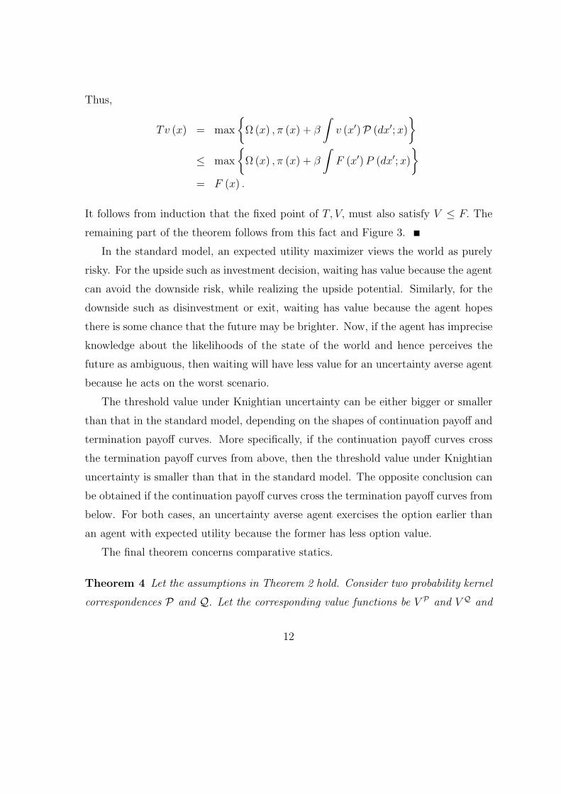
Thus,

Tv (x) = max

Ω (x) , π (x) + β

∫

v (x′)P (dx′; x)

≤ max

Ω (x) , π (x) + β

∫

F (x′) P (dx′; x)

= F (x) .

It follows from induction that the fixed point of T, V, must also satisfy V ≤ F. The

remaining part of the theorem follows from this fact and Figure 3.

In the standard model, an expected utility maximizer views the world as purely

risky. For the upside such as investment decision, waiting has value because the agent

can avoid the downside risk, while realizing the upside potential. Similarly, for the

downside such as disinvestment or exit, waiting has value because the agent hopes

there is some chance that the future may be brighter. Now, if the agent has imprecise

knowledge about the likelihoods of the state of the world and hence perceives the

future as ambiguous, then waiting will have less value for an uncertainty averse agent

because he acts on the worst scenario.

The threshold value under Knightian uncertainty can be either bigger or smaller

than that in the standard model, depending on the shapes of continuation payoff and

termination payoff curves. More specifically, if the continuation payoff curves cross

the termination payoff curves from above, then the threshold value under Knightian

uncertainty is smaller than that in the standard model. The opposite conclusion can

be obtained if the continuation payoff curves cross the termination payoff curves from

below. For both cases, an uncertainty averse agent exercises the option earlier than

an agent with expected utility because the former has less option value.

The final theorem concerns comparative statics.

Theorem 4 Let the assumptions in Theorem 2 hold. Consider two probability kernel

correspondences P and Q. Let the corresponding value functions be V P and V Q and

12

the corresponding threshold values be xP and xQ. If P (x) ⊂ Q (x) , then V P ≥ V Q.

Moreover, if the continuation payoff curves cross the termination payoff curves from

above (below), then xP ≥ (≤)xQ.

Proof. Define the operator TP : C (X) → C (X) by

TPv (x) = max

Ω (x) , π (x) + β

∫

v (x′)P (dx′; x)

, v ∈ C (X) .

Similarly, define an operator TQ : C (X) → C (X) corresponding to Q. Take any

functions v1, v2 ∈ C (X) such that v1 ≥ v2, it can be shown that TPv1 (x) ≥ TQv2 (x) .

By induction, the fixed points V P and V Q must satisfy V P ≥ V Q. The remaining

part of the theorem follows from Figure 4.

It is intuitive that the set of priors P (x) captures uncertainty aversion and the

degree of uncertainty aversion.8 A larger set of priors means that the agent has more

imprecise knowledge and is less confident to assign probabilities to the world. Hence,

he is more uncertainty averse. This theorem says that the option value is lower if the

agent is more uncertainty averse, and hence the agent exercises the option earlier.

4 Applications

This section applies our results to several widely studied examples, which include real

investment, job search, firm exit, firm default, and youth suicide.

4.1 Real Investment

A classic application of real-options approach is irreversible investment decisions.9

The standard real-options approach makes the analogy of corporate investment to

8See Gilboa and Schmeidler (1989) and Epstein (1999).9See Bernanke (1983), Brennan and Schwartz (1985), McDonald and Siegel (1985, 1986), Titman

(1986), Williams (1991), and Grenadier (1996) for important contributions. See Dixit and Pindyck

(1994) for a textbook treatment.

13

the exercising of an American call option on the underlying project. Once that

analogy is made, then we may apply the methodology developed in the financial

options literature to corporate investment problems. Formally, we follow McDonald

and Siegel (1986) and cast the investment problem into our framework by setting

Ω (x) = x − I, π (x) = 0,

where x represents the value of the project (for example, the real estate property

constructed on the land), and I represents the known and fixed investment cost to

develop the project (for example, construction cost).

The standard real-options model predicts that there is an option value of wait-

ing, because investment is irreversible and flexibility in timing has value. Empirical

evidence supports the option value of waiting in corporate investment. For example,

Summers (1987) finds that hurdle rates for investment range from 8 to 30 percent,

with a median of 15 percent and a mean of 17 percent, much higher than the com-

monly used risk-adjustment cost of capital.

Another main prediction of the standard real investment model is that an increase

in risk raises the option value and the investment threshold (see Pindyck and Dixit

(1994)). This derives from the fundamental insight behind the option pricing theory,

in that firms may capture the upside gains and minimizes the downside loss by waiting

for the risk of project value to be partially resolved.

While the standard real-options model predicts a monotonic relationship between

the investment threshold and the volatility of project value, our model makes an

important distinction between risk and uncertainty, and argues that risk (which can

be described by a single probability measure) and uncertainty (multiplicity of pri-

ors) have different effects on investment timing. Specifically, our model predicts that

Knightian uncertainty lowers option value of waiting (see Figure 5). This implies

that an uncertainty averse investor invests earlier than the standard expected utility

maximizer. The intuition is that the decision maker’s aversion to ambiguity leads

14

him to be more “pessimistic” about the expected future value of project by wait-

ing. Therefore, ambiguity aversion (Knightian uncertainty) has the opposite effect

on investment timing decision than risk does. The effect of ambiguity aversion thus

partially offsets the effect of risk on investment threshold.

4.2 Job Search

In job search models, a worker’s decision can be described by a stopping problem

(See Ljungqvist and Sargent (2000)). As an illustration, we present McCall’s (1970)

model. In each period, the worker has a job offer with wage x ∈ [0, B] ⊂ R drawn

from a fixed distribution. The worker has the option of rejecting the offer, in which

case he receives unemployment compensation c this period and waits until next period

to draw another offer. Alternatively, the worker can accept the offer to work at x, in

which case he receives a wage of x per period forever. Neither quitting nor firing is

permitted. This model can be cast into our framework by setting

Ω (x) =x

1 − β, π (x) = c.

A major prediction of McCall’s model is that an increase in risk in the sense of

mean-preserving spread raises the reservation wage.10 This means that a worker tends

to wait to get a higher wage offer in riskier situations. Again the intuition comes from

the option pricing theory that the value of an option is increasing in risk. However,

this model cannot explain the phenomenon that workers tend to accept low wages in

economic downturns where risk seems to be higher. Our theory offers an explanation.

In economic downturns, a worker is more ambiguous about job offers. He is less sure

about the likelihood of getting a job and obtaining favorable wages. Given that the

worker is uncertainty averse, our theory predicts that the value of the option is lower,

and hence the reservation wage is smaller in recessions than in expansions (see Figure

6). This also implies that the worker tends to accept job offers earlier in recessions.

10See Ljungqvist and Sargent (2000, p.92) for a proof.

15

4.3 Firm Exit

For the firm exit problem, the process (xt)t≥0 could be interpreted as a demand shock

or a productivity shock. Let the outside opportunity value be a constant γ ≥ 0.

Stay in business generates profits Π (x) > 0 and incurs a fixed cost cf > 0. Then the

problem fits into our framework by setting11

Ω (x) = γ, π (x) = Π (x) − cf .

According to the standard real options approach, the exit trigger point is lower

than that predicted by the textbook Marshallian net present value principle. This

implies that firms stay in business for lengthy periods while absorbing operating

losses. Only when the upside potential is bad enough, will the firm not absorb losses

and abandon operation. The standard real options approach also predicts that an

increase in risk in the sense of mean preserving spread raises the option value, and

hence lowers the exit trigger. This implies that firms should stay in business longer in

riskier situations, even though they suffer substantial losses. However, this prediction

seems to be inconsistent with the large amount of quick exit in IT industry in recent

years.

Our theory provides an explanation. In recent years, due to economic recessions,

firms are more ambiguous about the industry demand and their productivity. They

are less sure about the likelihoods of when the economy will recover. Intuitively, the

set of probability measures that workers may conceive is larger in recessions. Thus,

by Theorem 4, the value of the firm is lower and the exit trigger is higher. This

induces firms to exit earlier (see Figure 7).

11See Dixit (1989) for a continuous time model of entry and exit and Hopenhayn (1992) for a

dicrete time industry equilibrium model of entry and exit.

16

4.4 Firm Default

Let (xt)t≥0 be the cash flow process of the firm. Suppose the firm issues corporate

bond. The bond contract specifies a perpetual flow of coupon payments b to bond-

holders. The remaining cash flows from operation accrue to shareholders. If the firm

defaults on its debt obligations, it is immediately liquidated. Upon default, bond-

holders get the liquidation value and shareholders get nothing. Shareholders’ decision

is to choose a default time to maximize equity value. Default is determined by bond

covenants. If debt has positive net-worth covenants, then default occurs when the

firm’s net worth becomes negative. Alternatively, if debt has no protective covenants,

then default occurs only when the firm cannot meet the required coupon payment

by issuing additional equity: that is, when equity value falls to zero. Formally, the

default problem under unprotected debt covenants is similar to the exit problem (see

Figure 7) and can be cast into our framework by setting

Ω (x) = 0, π (x) = x − b.

According to the standard real options approach, the firm continues to meet

coupon payments even though it suffers losses.12 When the cash flow is low enough,

the firm defaults on its debt. Viewing equity value as an option, the standard model

also predicts that equity value increases with risk (volatility) of cash flows, and hence

the default boundary decreases with it. This implies that we should see less default

in recessions. However, as documented in Moody (2000), default rates are counter-

cyclical.

According to our theory, investors and firms are more ambiguous about the eco-

nomic prospects in recessions than in expansions. Thus, equity value is lower and

default boundary is higher in recessions than in expansions. Our theory immediately

delivers countercyclical default rates.

12See Leland (1994) for a single firm model and Miao (2003) for an industry equilibrium model.

See Huang and Huang (2003) for evidence.

17

The standard real options approach to corporate finance emphasizes the impor-

tance of credit risk in determining default rate, credit spread, and capital structure.

Our theory opens a new door for thinking about the determinant of these variables.

In particular, we argue that Knightian uncertainty is an important determinant.

4.5 Youth Suicide

There are two theories about economics of suicide. One is the Beckerian view, pro-

posed by Hamermesh and Soss (1974). They argue that an individual will commit

suicide when the expected life-time utility falls short of the benchmark utility level

that he receives from ending his life. However, this Beckerian view of the world ob-

viously ignores the option value of being alive. For example, the very poor might get

lucky and wins a big lottery. Dixit and Pindyck (1994) argue that Hamermesh-Soss

theory provide the individual agent with not enough rationality. Suicide (if success-

ful) is a completely irreversible decision and forgoes all the possible future up-side

scenarios. Naturally, option theory based argument suggests that the agent shall not

terminate his life simply based on the present value calculations as in Hamermesh and

Soss (1974). Conventional wisdom seems capture the option value of being alive very

well. For example, a famous Chinese saying (from ancient days) states that “Dying

with dignity is worse than surviving with misery.”

Undoubtedly, option value of being alive is crucial in the economics of suicide.

However, a standard real option theory also confronts empirical difficulties. Culter et

al. (2001) find that suicide rates are quite flat across individuals in all age groups.13

The almost constant suicide rate across different age groups poses a strong challenge

to the standard real-option explanation of suicide, because the young has a higher

expected life-time earnings than the old. Moreover, it is even harder to explain why

13For example, the suicide rates (in 1990) are 15 out of 100,000 for the age groups 20-24, 25-34,

35-44, and 45-54. The suicide rate is 21 out of 100,000, for age group 65+, slightly higher, most

likely due to health reasons and loneliness.

18

college students attempt and commit suicides. After all, college students are young

and have high expected future earnings opportunities.

Our theory provides an explanation to the observed high suicide rate among young

people, including college students. We argue that those who commit suicide are often

overly concerned about the prospects of their lives. They are not confident about their

future earnings prospect and the happiness of their future lives. In our language, there

is much greater perceived (Knightian) uncertainty in their minds. Thus, these young

individuals perceive very low option value of continuing to be alive, which possibly

motivates them to commit suicide.

We now formally map our theory to the suicide example. In order to capture the

differences in life expectancy between the young and the old in a simplest possible

setting, we adopt the perpetual-youth model of Yaari (1965) and Blanchard (1985).

Let py and po denote the survival probabilities per period for the young and the old,

respectively. Obviously, by definition, we have py > po. Then, the agent decides

whether to terminate his life by solving the following exit problem:

Vi(x) = max

γ, π (x) + βpi

∫

Vi(x′)Pi(dx′; x)

, (6)

where π (x) represents current earnings of being alive and γ is the level of utility

attained by ending one’s life, and where i = y and i = o stand for the “young” and

the “old”, respectively. We argue that the young agent who commits suicide has a

more pessimistic view of life. Formally, our model states that the set of priors Py

for the young who commit suicide is larger than the set of priors Po for the old, and

contains the pessimistic view of the world. Although the young has a higher discount

factor than the old (py > po), the value function Vy for the young may still be lower

than the value function Vo for the old, due to Po ⊂ Py (See Theorem 4).

Our model has interesting policy implications. Based on our theory, offering coun-

selling services to college students helps them lower their perceived level of Knightian

uncertainty, and thus reduces the set of priors. As a result, they will value their lives

19

less pessimistically.

5 Conclusion

Uncertainty plays an important role in real options problems. In standard mod-

els, there is no meaningful distinction between risk and uncertainty. To afford this

distinction, we have applied the multiple-priors utility model to analyze an option

exercise problem. We have shown that the option value under Knightian uncertainty

is smaller than that in the standard model. Moreover, an uncertainty averse agent ex-

ercises the option earlier than the standard expected utility maximizer. We have also

shown that if the agent is more uncertainty averse or faces a higher level of Knightian

uncertainty, then he exercises the option earlier. Several examples have revealed that

our model can explain some phenomena that are inconsistent with the predictions

of the standard model. Our model has a number of empirical implications. Further

empirical test should be urgent in the research agenda.

20

References

Anderson, E. W., L. P. Hansen and T. J. Sargent, 2003, A quartet of semigroups for

model specification, robustness, prices of risk, and model detection, Journal of

the European Economic Association, 1, 68-123.

Bernanke, B. S., 1983, Irreversibility, Uncertainty, and Cyclical Investment, Quar-

terly Journal of Economics, 98, 85-106.

Blanchard, O. J., 1985, Debt, deficits, and finite horizons, Journal of Political Econ-

omy, 93, 223-47.

Brennan, M. J., and E. S. Schwartz, 1985, Evaluating Natural Resource Investments,

Journal of Business, 58, 135-57.

Cao, H. H, T. Wang and H. H. Zhang, 2002, Model uncertainty, limited market

participation, and asset pricing, UBC.

Chen, Z. and L. G. Epstein, 2002, Ambiguity, risk and asset returns in continuous

time, Econometrica 4, 1403-1445.

Cutler, D. M., E. Glaeser and K. Norberg, 2000, Explaining the rise in youth suicide,

NBER working paper W7713.

Dixit, A., 1989, Entry and exit decisions under uncertainty, Journal of Political

Economy, 97, 620-638.

Dixit, A., 1992, Investment and hysteresis, Journal of Economic Perspectives 6,

107-132.

Dixit, A. and R. Pindyck, 1994, Investment Under Uncertainty, Princeton University

Press, Princeton, NJ.

21

Ellsberg, D., 1961, Risk, Ambiguity and the Savage Axiom, Quarterly Journal of

Economics 75, 643-669.

Epstein, L. G., 1999, A definition of uncertainty aversion, Review of Economic Stud-

ies 66, 579-608.

Epstein, L. G. and J. Miao, 2003, A two-person dynamic equilibrium under ambi-

guity, Journal of Economic Dynamics and Control 27, 1253-1288.

Epstein, L. G. and M. Schneider, 2002, Recursive multiple-priors, forthcoming in

Journal of Economic Theory.

Epstein, L. G. and T. Wang, 1994, Intertemporal asset pricing under Knightian

uncertainty, Econometrica 62, 283-322.

Epstein, L. G. and T. Wang, 1995, Uncertainty, risk-neutral measures and security

price booms and crashes, Journal of Economic Theory 67, 40-82.

Epstein, L. G. and J. Zhang, 2001, Subjective probabilities on subjectively unam-

biguous events, Econometrica 69, 265-306.

Gilboa, I. and D. Schmeidler, 1989, Maxmin expected utility with non-unique priors,

Journal of Mathematical Economics 18, 141-153.

Grenadier, S. R., 1996, The strategic exercise of options: development cascades and

overbuilding in real estate markets, Journal of Finance 51, 1653-1679.

Hamermesh, D. S. and N. M. Soss, 1975, An Economic Theory of Suicide, Journal

of Political Economy 82, 83-98.

Hansen, L. P. and T. J. Sargent, 2000, Acknowledging misspecification in macroe-

conomic theory, Sargent’s Frisch Lecture at the 2000 World Congress of the

Econometric Society.

22

Hopenhayn, H., 1992, Entry, exit, and firm dynamics in long run equilibrium, Econo-

metrica 60, 1127-1150.

Huang, J. and M. Huang, 2003, How much of the corporate treasury yield spread is

due to credit risk? working paper.

Knight, F., 1921, Risk, Uncertainty, and Profit, Boston: Houghton Mifflin.

Kogan, L. and T. Wang, 2002, A simple theory of asset pricing under model uncer-

tainty, working paper.

Leland, H. E., 1994, Corporate debt value, bond covenants and optimal capital

structure, Journal of Finance 49, 1213-1252.

Ljungqvist, L. and T. J. Sargent, 2000, Recursive Macroeconomic Theory, MIT

Press.

McCall, J., 1970, Economics of information and job search, Quarterly Journal of

Economics 84, 113-126.

McDonald, R. and D. Siegel, 1985, Investment and the valuation of firms when there

is an option to shut down, International Economic Review 26, 331-349.

McDonald, R. and D. Siegel, 1986, The value of waiting to invest, Quarterly Journal

of Economics 101, 707-728.

Miao, J., 2003, Optimal capital structure and industry dynamics, Working paper,

Boston University.

Moody, 2000, Historical default rates of corporate bond issuers, 1920-1999, Moody’s

Investors Service.

Routledge, B. and S. Zin, 2003, Model uncertainty and liquidity, NBER working

paper 8683.

23

Stokey, N. and R. E. Lucas with E. C. Prescott, 1989, Recursive Methods in Eco-

nomic Dynamics, Cambridge, MA: Harvard University Press.

Summers, L. H., 1987, Investment Incentives and the Discounting of Depreciation

Allowances, in The Effects of Taxation on Capital Accumulation, Martin Feld-

stein, ed., Chicago, University of Chicago Press.

Titman, S., 1985, Urban land prices under uncertainty, American Economic Review,

75, 505-14.

Williams, J. T., 1991, Real estate development as an option, Journal of Real Estate

Finance and Economics 4, 191-208.

Yaari, M. E., Uncertain lifetimes, life insurance, and the theory of the consumer,

Review of Economic Studies, 32, 137-50.

24

x∗x∗

Ω(x)

Ω(x) F (x)

F (x)

stoppingstopping continuationcontinuation

Figure 2: The value function and exercising threshold in the standard model.

25

x∗ x∗∗x∗x∗∗

Ω(x)

Ω(x)

F (x)F (x)

V (x)

V (x)

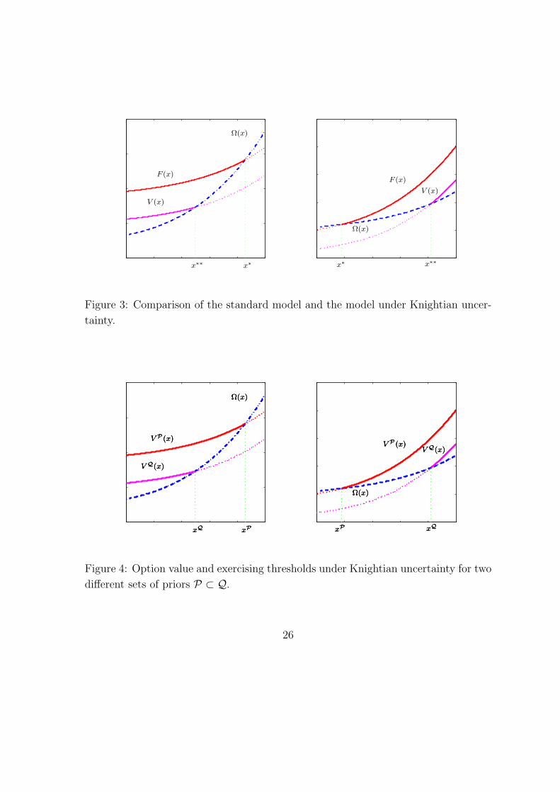
Figure 3: Comparison of the standard model and the model under Knightian uncer-

tainty.

xPxPxP xQxQxQxPxPxPxQxQxQ

Ω(x)Ω(x)Ω(x)

Ω(x)Ω(x)Ω(x)

V P (x)V P (x)V P (x)V P (x)V P (x)V P (x)

V Q(x)V Q(x)V Q(x)

V Q(x)V Q(x)V Q(x)

Figure 4: Option value and exercising thresholds under Knightian uncertainty for two

different sets of priors P ⊂ Q.

26

x∗x∗x∗∗x∗∗

F (x)F (x)

V (x)V (x)

x − Ix − I

II

Figure 5: Investment timing under Knightian uncertainty and in the standard model.

The upper (dashed) curve corresponds to the value function F (x) in the standard

model. The lower (solid) curve corresponds to the value function V (x) under Knigh-

tian uncertainty.

27

x1−β

x1−β

x1−β

x1−β

x1−β

x1−β

V P (x)V P (x)V P (x)V P (x)V P (x)V P (x)

V Q(x)V Q(x)V Q(x)V Q(x)V Q(x)V Q(x)

xPxPxPxPxPxPxQxQxQxQxQxQ

Figure 6: Job search under different degrees of Knightian uncertainty. The upper

(solid) curve corresponds to the value function V P(x) and the lower (solid) curve

corresponds to the value function V Q(x) where P ⊂ Q.

28

V P (x)

V Q(x)

xQxP

Figure 7: Firm Exit/Default under different degrees of Knightian uncertainty. The

upper (dashed) curve corresponds to the value function V P(x) and the lower (solid)

curve corresponds to the value function V Q(x) where P ⊂ Q.

29