river temperature behaviour in changing environments...
TRANSCRIPT
Erasmus Mundus Joint Doctorate School in Science for MAnagement of
Rivers and their Tidal System
Roshni Arora
River temperature behaviour in changing
environments: trends, patterns at different spatial and
temporal scales and role as a stressor
2015

This thesis work was conducted during the period 1st October 2012 - 15
th
December 2015, under the supervision of Dr. Markus Venohr (Leibniz
Institute of Freshwater Ecology and Inland Fisheries Berlin), Dr. Martin T.
Pusch (Leibniz Institute of Freshwater Ecology and Inland Fisheries Berlin),
Dr. Marco Toffolon (University of Trento, Italy) and Dr. Klement Tockner
(Freie Universität Berlin) at Freie Universität Berlin, University of Trento,
Italy and Leibniz Institute of Freshwater Ecology and Inland Fisheries
Berlin.
1st Reviewer: Prof. Dr. Klement Tockner
2nd
Reviewer: Prof. Dr. Gunnar Nützmann
Date of defence: 15.02.2016

The SMART Joint Doctorate Programme
Research for this thesis was conducted with the support of the Erasmus
Mundus Programme1, within the framework of the Erasmus Mundus Joint
Doctorate (EMJD) SMART (Science for MAnagement of Rivers and their
Tidal systems). EMJDs aim to foster cooperation between higher education
institutions and academic staff in Europe and third countries with a view to
creating centres of excellence and providing a highly skilled 21st century
workforce enabled to lead social, cultural and economic developments. All
EMJDs involve mandatory mobility between the universities in the consortia and lead to the award of recognised joint, double or multiple degrees.
The SMART programme represents a collaboration among the University of
Trento, Queen Mary University of London, and Freie Universität Berlin.
Each doctoral candidate within the SMART programme has conformed to the following during their 3 years of study:
(i) Supervision by a minimum of two supervisors in two institutions
(their primary and secondary institutions).
(ii) Study for a minimum period of 6 months at their secondary
institution
(iii) Successful completion of a minimum of 30 ECTS of taught
courses
(iv) Collaboration with an associate partner to develop a particular
component / application of their research that is of mutual
interest.
(v) Submission of a thesis within 3 years of commencing the
programme.
1 This project has been funded with support from the European Commission. This
publication reflects the views only of the author, and the Commission cannot be held responsible for any use which may be made of the information contained therein

I
Table of Contents
Table of Contents ................................................................................................. I
Summary ............................................................................................................ IV
Zusammenfassung ........................................................................................... VII
Thesis outline ..................................................................................................... XI
List of Tables .................................................................................................. XIV
List of Figures ................................................................................................ XVII
1. General introduction ....................................................................................... 1
1.1 River temperature: importance in ecosystem functioning and research
history .............................................................................................................. 1
1.2 Processes and controls determining river temperatures ......................... 3
1.3 Changing river temperatures in changing environments and its
implications ..................................................................................................... 5
1.4 Research gaps, aims and structure of the thesis ..................................... 8
2. Changing river temperatures in Northern Germany: trends and
drivers of change ................................................................................................ 11
2.1 Abstract ................................................................................................... 11
2.2 Introduction............................................................................................. 12
2.3 Materials and methods ........................................................................... 17
2.4 Results ..................................................................................................... 21
2.5 Discussion ............................................................................................... 29
2.6 Conclusion .............................................................................................. 35
3. Influence of landscape variables in inducing reach-scale thermal
heterogeneity in a lowland river ...................................................................... 38
3.1 Abstract ................................................................................................... 38
3.2 Introduction............................................................................................. 38
II
3.3 Materials and methods ........................................................................... 41
3.4 Results ..................................................................................................... 53
3.5 Discussion ............................................................................................... 69
3.6 Conclusion .............................................................................................. 73
4. Interactions between effects of experimentally altered water
temperature, flow and dissolved oxygen levels on aquatic invertebrates . 75
4.1 Abstract ................................................................................................... 75
4.2 Introduction............................................................................................. 76
4.3 Materials and methods ........................................................................... 83
4.4 Results ..................................................................................................... 86
4.5 Discussion ............................................................................................... 92
4.6 Conclusion .............................................................................................. 96
5. GENERAL DISCUSSION ........................................................................... 98
5.1 Rationale and research aims .................................................................. 98
5.2 Key research findings ............................................................................. 99
5.3 Synthesis ............................................................................................... 101
5.4 Implications for river ecosystem management ................................... 103
References ......................................................................................................... 107
Statement of academic integrity .................................................................... 123
Acknowledgements .......................................................................................... 124
APPENDIX A: Supplementary material for Chapter 2 ............................ 126
APPENDIX B: Supplementary material for Chapter 3 ............................ 133
APPENDIX C: Heat Flux Equations used in Chapter 3 ........................... 136

III
Summary
IV
Summary
River/stream water temperature is one of the master water quality parameters
as it controls several key biogeochemical, physical and ecological processes
and river ecosystem functioning. Thermal regimes of several rivers have
been substantially altered by climate change and other anthropogenic
impacts resulting in deleterious impacts on river health. Given its
importance, several studies have been conducted to understand the key
processes defining water temperature, its controls and drivers of change.
Temporal and spatial river temperature changes are a result of complex
interactions between climate, hydrology and landscape/basin properties,
making it difficult to identify and quantify the effect of individual controls.
There is a need to further improve our understanding of the causes of
spatiotemporal heterogeneity in river temperatures and the governing
processes altering river temperatures. Furthermore, to assess the impacts of
changing river temperatures on the river ecosystem, it is crucial to better
understand the responses of freshwater biota to simultaneously acting
stressors such as changing river temperatures, hydrology and river quality
aspects (e.g. dissolved oxygen levels). So far, only a handful of studies have
explored the impacts of multiple stressors, including changing river
temperature, on river biota and, thus, are not well known.
This thesis, thus, analysed the changes in river temperature behaviour at
different scales and its effects on freshwater organisms. Firstly, at a regional
scale, temporal changes in river temperature within long (25 years) and short
time periods (10 years) were quantified and the roles of climatic,
hydrological and landscape factors were identified for North German rivers.
Secondly, at a reach scale, spatial temperature heterogeneity in a sixth-order
lowland river (River Spree) was quantified and the role of landscape factors
in inducing such heterogeneity was elucidated. Thirdly, at a site scale, short-
term behavioural responses (namely drift) of three benthic invertebrate
species to varying levels of water temperature, flow, and dissolved oxygen,
and to combinations of those factors were experimentally investigated.
Results from this thesis showed that, at a regional scale, the majority of
investigated rivers in Germany have undergone significant annual and
seasonal warming in the past decades. Air temperature change was found to
Summary
V
be the major control of increasing river temperatures and of its temporal
variability, with increasing influence for increasing catchment area and lower
altitudes (lowland rivers). Strongest river temperature increase was observed
in areas with low water availability. Other hydro-climatological variables
such as flow, baseflow, NAO, had significant contributions in river
temperature variability. Spatial variability in river temperature trend rates
was mainly governed by ecoregion, altitude and catchment area via affecting
the sensitivity of river temperature to its local climate. At a reach scale as
well, air temperature was the major control of the temporal variability in
river temperature over a period of nine months within a 200 km lowland
river reach. The spatial heterogeneity of river temperature in this reach was
most apparent during warm months and was mainly a result of the local
landscape settings namely, urban areas and lakes. The influence of urban
areas was independent of its distance from the river edge, at least when
present within 1 km. Heat advected from upstream reaches determined the
base river temperature while climatological controls induced river
temperature variations around that base temperature, especially below lakes.
Riparian buffers were not found to be effective in substantially moderating
river temperature in reaches affected by lake warming due to the dominant
advected heat from the upstream lake. Experimental investigation indicated
that increasing water temperature had a stronger short-term effect on
behavioural responses of benthic invertebrates, than simultaneous changes in
flow or dissolved oxygen. Also, increases in water temperature was shown to
affect benthic invertebrates more severely if accompanied by concomitant
low dissolved oxygen and flow levels, while interactive effects among
variables vary much among taxa.
These results support findings of other studies that river warming, similar to
climate change, might be a global phenomenon. Within Germany, lowland
rivers are the most vulnerable to future warming, with reaches affected by
urbanization and shallow lentic structures being more vulnerable and,
therefore, requiring urgent attention. Furthermore, river biota in lowland
rivers is particularly susceptible to short-term increases in river temperature
such as heat waves. Plantation of riparian buffers, a widely recognized
practice to manage climate change effects, in the headwater reaches can be
suggested to mitigate and prevent future warming of lowland rivers in
general and also throughout river basins, as river temperature response in
Summary
VI
lowland catchments is a culmination of local and upstream conditions.
However, further river temperature increase in lowland river reaches within
or close to urban areas and shallow lentic structures will be more difficult to
mitigate only via riparian shading and would require additional measures.
Zusammenfassung
VII
Zusammenfassung
Die Wassertemperatur ist ein zentraler Wasserqualitätsparameter, der eine
Vielzahl verschiedener biogeochemischer, physischer und ökologischer
Prozesse sowie Ökosystemfunktionen von Flüssen steuert. Das
Temperaturregime vieler Flüsse wurde bereits nachhaltig durch
Klimawandel und andere anthropogene Einflüsse verändert und beeinflusst
den chemischen und ökologischen Zustand der Flüsse. Angesichts dieser
Bedeutung, haben bereits mehrere Studien die beteiligten Prozesse,
Steuergrößen und anthropogenen Überprägungen der Wassertemperatur
untersucht. Zeitliche und räumliche Temperaturänderungen resultieren aus
einer komplexen Wechselwirkung zwischen Klima, Hydrologie und
Einzugsgebietseigenschaften. Die Identifikation und Quantifizierung der
Effekte einzelner Steuergrößen ist dementsprechend schwierig. Trotz
früherer Studien besteht ein weiterer Forschungsbedarf um die Ursachen der
raum-zeitlichen Heterogenität von Wassertemperaturen und ihrer
maßgebenden Steuerungsprozesse vollständig zu verstehen. Darüber hinaus
ist es entscheidend die Reaktionen von Süßwasserorganismen auf
gleichzeitig wirkende Stressoren wie veränderte Wassertemperatur,
Hydrologie und Wasserqualitätsaspekte (z.B. Gehalt an gelöstem Sauerstoff)
besser zu verstehen um die Bedeutung von Temperaturregimeänderungen
vollständig erfassen zu können. Bisher haben nur wenige Studien die
Auswirkungen multipler Stressoren, einschließlich der Änderung der
Wassertemperatur, auf Süßwasserorganismen untersucht.
Die vorliegende Arbeit adressiert sowohl Temperaturregimeänderungen als
auch deren Wirkung auf Süßwasserorganismen auf verschiedenen Skalen.
Im ersten Teil werden regionale Wassertemperaturänderungen für lange (25
Jahre) und kurze Zeiträume (10 Jahre) quantifiziert. Dabei werden die
Bedeutung von Klima, Hydrologie und Einzugsgebietseigenschaften für
Flüsse im Norddeutschen Tiefland identifiziert. Im zweiten Teil der Arbeit
wird die Heterogenität zwischen Wassertemperaturänderungen einzelner
Flussabschnitte der Spree quantifiziert und mit verschiedenen
Einzugsgebietseigenschaften in Bezug gesetzt. Im dritten Teil werden
kurzfristige Verhaltensreaktionen (Drift) von drei benthischen wirbellosen
Arten, aufgrund einzelner und kombinierter Änderungen von
Zusammenfassung
VIII
Wassertemperatur, Strömung und dem Gehalt von gelöstem Sauerstoffs
experimentell untersucht.
Die Ergebnisse der vorliegenden Arbeit zeigen, dass auf regionaler Ebene,
die Mehrheit der untersuchten Flüsse in Deutschland in den vergangenen
Jahrzehnten einer signifikanten jährlichen als auch saisonalen Erwärmung
unterlag. Die Veränderung der Lufttemperatur ist hierbei die
Hauptsteuergröße veränderter Wassertemperaturen und ihrer zeitlichen
Variabilität, wobei der Einfluss mit der Einzugsgebietsgröße und tieferen
Lagen (Tieflandflüsse) zunimmt. Die stärkste Zunahme der
Wassertemperatur wurde in Gebieten mit geringer Wasserverfügbarkeit
festgestellt. Aber auch andere hydroklimatische Parameter wie Abfluss,
Basisabfluss, NAO, haben einen signifikanten Einfluss auf die Variabilität
der Wassertemperatur. Die räumliche Variabilität der
Temperaturänderungsraten in Flüssen wird hauptsächlich durch die
Klimasensitivität eines Gewässers bestimmt und durch die Ökoregion, Höhe
und Einzugsgebietsgröße beschrieben. Auch für den 200 km langen
Abschnitt der Spree erklärte, während eines neun-monatigen
Messprogramms, die Lufttemperatur maßgeblich die zeitliche Variabilität
der Wassertemperatur. In dem untersuchten Abschnitt der Spree wird die
räumliche Heterogenität der Wassertemperatur, insbesondere während der
warmen Monate, im Wesentlichen durch die lokalen Gegebenheiten (urbane
Gebiete und Seen) erklärt. Der Einfluss urbaner Gebiete konnte hierbei
unabhängig von der jeweiligen Entfernung (max. 1 km) vom Flussufer
festgestellt werden. Insbesondere unterhalb von Seen, wird die mittlere
Wassertemperatur eines Gewässerabschnitts hauptsächlich durch die
advektiv mit dem Abfluss zugeführte Wärme bestimmt, wohingegen
Schwankungen um die mittlere Temperatur maßgeblich durch
klimatologische Größen gesteuert werden. Hierbei zeigte sich, dass in
Gewässerabschnitten unterhalb von Seen, die advektiv zugeführte Wärme,
deutlich dominiert und das Vorhandensein von Gewässerrandstreifen die
Wassertemperatur nicht nachweisbar beeinflussen. Die experimentellen
Untersuchungen ergeben, dass steigende Wassertemperaturen eine stärkere
kurzfristige Änderung der Verhaltensreaktionen des Makrozoobenthos
bewirken, als die gleichzeitige Änderung von Abfluss und Sauerstoffgehalt.
Die Wirkung erhöhter Wassertemperaturen in Kombination mit geringen
Zusammenfassung
IX
Sauerstoffgehalten oder Abflüssen fiel in der Regel stärker aus, unterschied
sich in seiner Wirkung jedoch teilweise erheblich zwischen den Arten.
Diese Ergebnisse unterstützen Aussagen anderer Studien, dass die
Wassertemperaturerhöhung in Flüssen, ähnlich wie der Klimawandel, ein
globales Phänomen ist. In Deutschland sind Tieflandflüsse, insbesondere
wenn sie urban geprägt sind oder flache Seen enthalten, am ehesten für einen
Temperaturanstieg empfänglich. Sie stellen somit besonders gefährdete
Systeme dar und benötigen einer besonderen Aufmerksamkeit. Darüber
hinaus sind Süßwasserorganismen in Tieflandflüssen besonders anfällig für
einen kurzfristigen Anstieg der Wassertemperatur durch beispielsweise
Hitzewellen. Der Effekt von Gewässerrandstreifen zur Abschwächung von
klimawandelbedingten Wassertemperaturanstiegen ist hinlänglich bekannt.
Dabei können sich Gewässerrandstreifen im Oberlauf nicht nur lokal positiv
auf das Temperaturregime, sondern auch auf unterhalb gelegene
Gewässerabschnitte auswirken. Die Minderung eines zukünftigen
Wassertemperaturanstieges in urbanen und durch Flachseen geprägten
Tieflandflüssen mittels Gewässerrandstreifen ist schwer erreichbar und wird
die Implementierung weiterer Maßnahmen erfordern.

Zusammenfassung
X
XI
Thesis outline
This thesis is composed of three manuscripts that are either accepted for
publication, or ready to be submitted to peer-reviewed journals. Each
manuscript has an introduction, methodology, results and discussion and
forms a chapter of the thesis. A general introduction section provides the
general context of the thesis and the results are discussed coherently as the
general discussion section. The layout of the three manuscripts was modified
and figures and tables were renumbered through the text to ensure a
consistent layout throughout the entire thesis. The references of the general
introduction, each manuscript, and general discussion were merged in an
overall reference section. The research aims of Chapters 2, 3 and 4 are
described in Paragraph 1.4.
Chapter 1:
General introduction
Chapter 2:
Arora R, Tockner K, Venohr M. (submitted to Hydrological Processes).
Changing river temperatures in Northern Germany: trends and drivers of
change.
Author Contributions:
R. Arora designed the study, analysed the data and compiled the manuscript.
K. Tockner and M. Venohr co-designed the study and contributed to the text.
Chapter 3:
Arora R, Toffolon M, Tockner K, Venohr M. (to be submitted) Influence of
landscape variables in inducing reach-scale thermal heterogeneity in a
lowland river.
Author Contributions:
R. Arora designed the study, organized and performed field work, analysed
the data and compiled the manuscript. M. Toffolon and M. Venohr co-
XII
designed the study and contributed to the text. K. Tockner co-designed the
study.
Chapter 4:
Arora R, Pusch MT, Venohr M. (to be submitted) Interactions between
effects of experimentally altered water temperature, flow and dissolved
oxygen levels on aquatic invertebrates.
Author Contributions:
R. Arora designed the study, organized and performed field and laboratory
work, analysed the data and compiled the manuscript. M.T. Pusch co-
designed the study and contributed to the text. M. Venohr co-designed the
study.
Chapter 5:
General discussion

XIII
XIV
List of Tables
Table II.1 Recent studies on river temperature trends worldwide (updated
from Kaushal et al., 2010) …………………………………………………15
Table II.2 Datasets used in the analysis with river temperature (RT), air
temperature (AT) and flow (Q) data...……………………………………...18
Table II.3 Mean (±S.E.) of significant seasonal river temperature (RT) and
air temperature (AT) trends during 1985-2010…………………….……….25
Table SII.1 Mean (±S.E.) of significant river temperature trends in the
different ecoregions and river types in Germany………………………….130
Table SII.2. Mean (±S.E.) of river temperature trends shown for the two
datasets (DS I and II) used in the study for different time periods. *Decadal
analysis for DS I was done at sites with significant river temperature trends
during 1985-2010………………………………………..………………..132
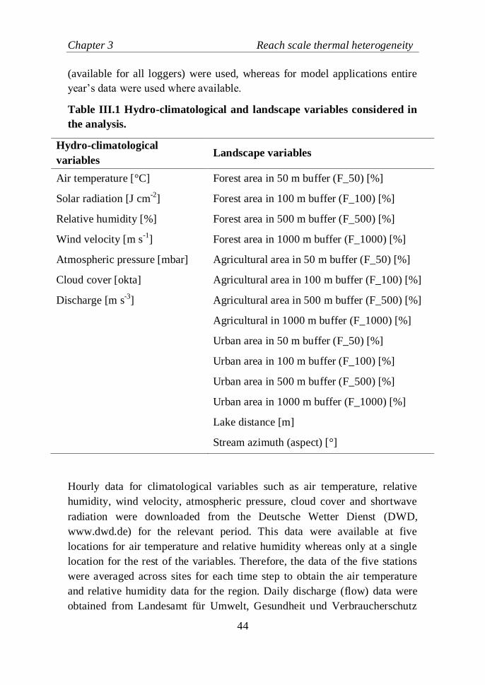
Table III.1 Hydro-climatological and landscape variables considered in the
analysis………………………………………………………………..……44
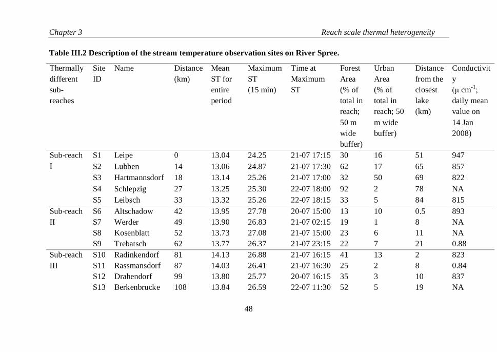
Table III.2 Description of the stream temperature observation sites on River
Spree………………………………………………………………………..48
Table III.3 Correlations of parameter C4 (air2stream), mean stream
temperature (for the entire period), mean 𝐸𝑟(for the entire period) with
landscape variables (LV). NS stands for not significant correlations……....60
Table III.4 Significant correlations between landscape variables (LV, see
Table 3.1) and mean (bold), maximum (italic) monthly STs for all sites. NS
stands for “not significant” correlations. P-values for significant correlations
are provided within the brackets………………………………………..…..64
Table III.5 Significant correlations between landscape variables (LV, see
Table 3.1) and mean monthly 𝐸𝑟 for all sites. NS stands for “not significant”
XV
correlations. P-values for significant correlations are provided within the
brackets……………………………………………………….…………….65
Table IV.1 Review of recent studies on the relative impacts of water
temperature (WT) compared to various water quality variables on freshwater
macro-invertebrates…………………………………………………………81
Table IV.2 Experimental levels of the aquatic variables subjected on macro-
invertebrate species to determine their responses…………..……………....85

XVI
XVII
List of Figures
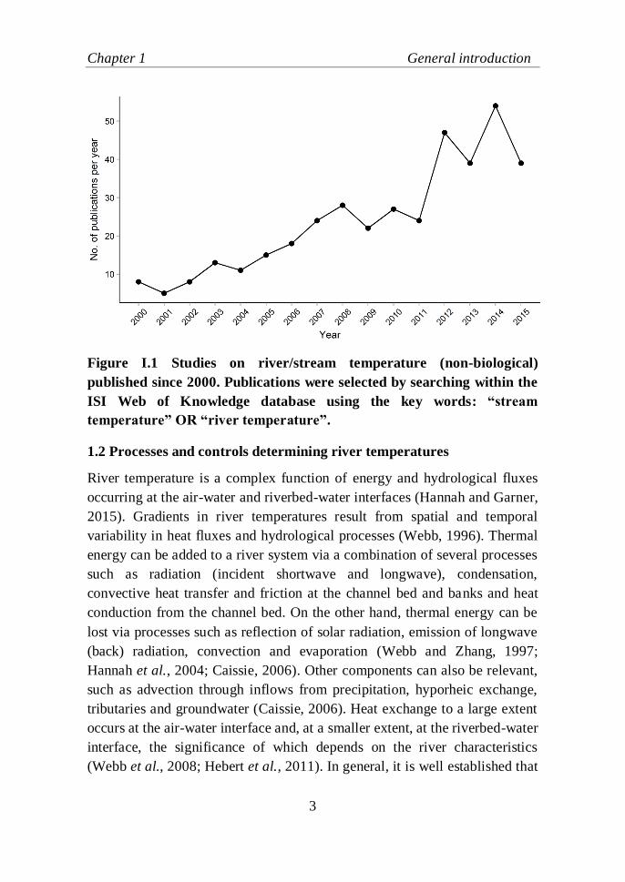
Figure I.1 Studies on river/stream temperature (non-biological) published
since 2000. Publications were selected by searching within the ISI Web of
Knowledge database using the key words: “stream temperature” OR “river
temperature”……………………………………………….…………………3
Figure II.1 Cumulative frequency distribution of river temperature trends at
a) all sites b) sites with significant trends for time periods 1985-2010 and
2000-2010. DS stands for dataset………………...………………………...22
Figure II.2 Significant temperature trends (°C year-1
) for time periods 1985-
2010 and 2000-2010 in six river basins in Germany. For 2000-2010, the sites
have been sorted into NE and NW sites. The common boundary of the Elbe
and Weser basin is the key differentiation point between north-eastern and
north-western regions………………………………………………………23
Figure II.3 Boxplots showing significant river temperature (RT) trends (left)
and coefficient of determination (R2) (right) from AT-RT regression
(original and deseasonalized (ds)) for NE and NW regions of Germany
during a) 1985-2010 and b) 2000-2010. NE region of Germany includes sites
within Elbe, Trave, Warnow and Odra river basins while the NW region of
Germany includes sites within Weser, Ems and Eider river basins. The mean
values of trends and R2 are shown by the square point……..………………24
Figure II.4 Mean (±S.E.) R2 values of significant correlations between
hydro-climatological variables and river temperature for original and
deseasonalized (ds) series, where applicable. Hydro-climatological variables
included are air temperature (AT), flow (Q), baseflow (BF) and North
Atlantic Oscillation Index (NAOI)…………………...………………….…27
Figure II.5 Boxplots showing the significant river temperature (RT) trends in
the relevant ecoregions. The mean RT trend is shown by the square point...28
Figure SII.1 Boxplots showing significant river temperature (RT) trends for
two decades. DS stands for dataset, where DS I (total n=132) are sites
analysed for 1985-2010 and DS II (total n=475) are sites analysed for 2000-
2010……………………………………………..……………………..….126
XVIII
Figure SII.2 Cumulative frequency distribution (ecdf) for proportion of
forest, agriculture and urban land use cover types within 1 km2 site buffers
(time period:2000-2010; n=112)………………………………………......127
Figure SII.3 Cumulative frequency distribution of significant air temperature
(AT)-river temperature (RT) slopes from linear regression for both time
periods……………………………………………………………………..128
Figure SII.4 Frequency of months with mean monthly river temperature
above the threshold temperature of 22°C plotted for several sites. The
threshold temperature was based on thermal limits of fish and invertebrate
species as mentioned in Hardewig et al. (2004), Haidekker & Hering (2008)
and Vornanen et al. (2014)…………………...…………………………...129
Figure III.1 Maps showing the location of the study area, stream temperature
(ST) measuring locations, and the thermally heterogeneous sub-reaches.
Stream temperature measuring locations are numbered corresponding to their
IDs (Table 3.2)………………………………………………….…………..43
Figure III.2 Daily means for the 4th
(blue), 10th (dark green) and 15
th (black)
day of each month plotted for the 20 sites on River Spree for all months
during the study period…………………………………………………..…55
Figure III.3 Boxplots showing 𝐸𝑟 values for the entire study period (a), for
the warmer months (b; June-Sep) and for the colder months (c; Jan-May) at
all reaches on River Spree. Mean values are represented by blue points.
Boxes around the median line show the 25th and 75th percentiles with
whiskers representing the 5th and 95th percentiles and each cross
representing the upper and lower outliers………..………………………....57
Figure III.4 Simulations of ST at site S9 (downstream) using ST at S6 as
input under the Lagrangian (green line) and local “Eulerian” framework
(blue line). The simulation was done for three solar radiation conditions:
actual (~70%; a), null (0%; b) and all (100%; c)…………………………...58
Figure III.5 Values of coefficient of determination (R2) from linear
regression (for air temperature, relative humidity) and non-linear models (for
solar radiation, atmospheric pressure, wind, cloud cover, discharge) between
XIX
daily mean hydroclimatological variables and ST for all sites on River
Spree………………………………………………………………………..61
Figure III.6 Root Mean Square Errors (RMSE) for the three models for all
sites on River Spree………………………..…………………………….....68
Figure III.7 Spatial variation of the air2stream parameters. Plots show the
ratios of the main model parameters to 𝑐3 (𝐶1, 𝐶2, 𝐶3, 𝐶4; see equation 8)...58
Fig. SIII.1 Share of cover of different land use types within 50, 100, 500 and
1000 m buffer widths at all sites on River Spree……………..………...…133
Fig. SIII.2 Daily range (maximum-minimum) for the 15th day of each month
plotted for 20 sites on River Spree for all months…………...…………....134
Fig. SIII.3 Plots showing the nature of relationship of ST with different
atmospheric variables. The curves were determined by the non-linear models
using the spline-smoothing function (function gam in mgcv package, R)..135
Figure IV.1 Sketch of the experimental flume……………………..…….…84
Figure IV.2 Interaction plot of flow and DO for the three study species
showing the mean number of detached individuals (average for the three
replicates ± SE, n=10 for D. haemobaphes and H.pellucidula; n=9 for C.
splendens)……………………………………………………………....…..87
Figure IV.3 Interaction plot of water temperature and DO for the three study
species showing the mean number of detached individuals (average for the
three replicates ± SE, n=10 for D. haemobaphes and H.pellucidula; n=9 for
C. splendens)…………………………………………………………….….89
Figure IV.4 Interaction plot of water temperature and flow for the three study
species showing the mean number of detached individuals (average for the
three replicates ± SE, n=10 for D. haemobaphes and H.pellucidula; n=9 for
C. splendens)………………………………………………………………..91
Figure IV.5 Interaction plot of temperature and flow at low DO level (< 2
mg/l) for H. pellucidula showing the number of individuals detached and the
XX
number of individuals showing respiratory undulations (average for the three
replicates ± SE, n=7)……………..................................................................92
Figure V.1 Synthesis of the findings from the thesis showing the major
variables affecting river thermal regime and, thereby, the freshwater
ecosystem. Climatic drivers such as air temperature exert major controls on
river temperature and act at regional scales while hydrological controls, such
as flow, act sub-regionally, having a substantial influence on river
temperature variability. Landscape and catchment properties induce local
and sub-regional spatial differences in climate, hydrology and river
morphology and thereby, river thermal regimes. Global changes caused by
human activities can affect river thermal regimes directly as well indirectly
via affecting any one or more of the mentioned controls. Extremes in river
temperatures and other important water quality parameters, such as flow and
dissolved oxygen, due to such environmental changes, can induce several
behavioural responses in freshwater species, ultimately affecting the entire
ecosystem as a whole……………………………………………….……..104

XXI
Chapter 1 General introduction
1
1. General introduction
1.1 River temperature: importance in ecosystem functioning and
research history
Rivers are hierarchical systems (Montgomery, 1999) in which physical
variables such as water temperature, channel area, velocity, flow volume, are
present in a continuous gradient of conditions (river continuum concept,
Vannote et al., 1980). Among these various variables, river temperature is a
physical property of prime importance as it controls physicochemical and
ecological processes within freshwater ecosystems. River/stream
temperature2 strongly governs the distribution, abundance (Haidekker and
Hering, 2008; Wenger et al., 2011a) and life cycle characteristics such as
growth, emergence, metabolism and survivorship (Watanabe et al., 1999;
Chadwick and Feminella, 2001, Schindler et al., 2005; Wehrly et al., 2007)
of freshwater species. It also controls river metabolism rates (Young and
Huryn, 1996; Alvarez and Nicieza, 2005), trophic relationships (Kishi et al.,
2005) and food web composition (Woodward et al., 2010b) within rivers. It
has a major influence on physical characteristics such as vapour pressure,
surface tension, density and viscosity (Stevens et al., 1975) and chemical
reaction rates (Brezonik, 1972), which in turn influence primary production
and decomposition rates (Friberg et al., 2009; Dang et al., 2009; Woodward
et al., 2010a). These processes consequently influence dissolved oxygen
concentrations (Sand-Jensen and Pedersen, 2005), nutrient cycling
(Ducharne, 2008) and litter processing (Bärlocher et al., 2008); all of which
contribute to river ecosystem health (Norris and Thoms, 1999). Given its
importance, it is crucial to have a clear understanding of the dynamics of
river temperature behaviour (Caissie, 2006).
First reported river temperature measurements date back to 1799, which
were made on the River Nile during the Napoleonic expedition to Egypt
(Webb et al., 2008). Earliest scientific studies on river temperature appeared
around 1960 and mainly aimed to understand the influence of river water
2 Throughout the thesis, the terms river temperature and stream temperature have been used
synonymously
Chapter 1 General introduction
2
temperature on the habitat use and occurrence patterns of cold-water adapted
fishes such as salmonids (Benson, 1953; Gibson, 1966; Edington, 1966), the
factors governing river thermal processes (Macan, 1958; Ward, 1963), the
effects of forest harvesting on river temperature (Gray and Edington, 1969;
Brown and Krygier, 1970) and to predict river temperature using heat
balance models (Brown, 1969; Morse, 1970). Ever since, the number of river
temperature studies has continuously increased, particularly after 1990
(Hannah et al., 2008b; Fig. I.1). Much of the research until now has focused
on understanding river temperature behaviour, direct/indirect impacts of
environmental change on river temperature and river temperature modelling
(Hannah et al., 2008b). More recently, exploring the past and future trends of
river temperature and the influence of climate change and human impacts on
these trends has gained interest (Webb et al., 2008; Isaak et al., 2012; Orr et
al., 2014; Rice and Jastram, 2015). Several reviews of river temperature
research exist in literature. These reviews give a gist of physical processes
and controls driving river temperature variability (Smith 1972; Ward 1985;
Caissie, 2006), advances in water temperature modelling (Caissie, 2006;
Benyahya et al., 2007), natural drivers and human modifications of river
temperature (Poole and Berman, 2001; Caissie, 2006), impacts of forest
removal (Moore et al., 2005), thermal heterogeneity and past/future changes
in river temperature in general (Webb et al., 2008) and advances in river
temperature research in United Kingdom (Hannah and Garner, 2015). These
reviews clearly highlight the need to further improve our understanding of
the spatial and temporal variability in river temperatures and the underlying
governing processes of river temperature change, in order to prevent
freshwater ecosystems from further degradation.
Chapter 1 General introduction
3
Figure I.1 Studies on river/stream temperature (non-biological)
published since 2000. Publications were selected by searching within the
ISI Web of Knowledge database using the key words: “stream
temperature” OR “river temperature”.
1.2 Processes and controls determining river temperatures
River temperature is a complex function of energy and hydrological fluxes
occurring at the air-water and riverbed-water interfaces (Hannah and Garner,
2015). Gradients in river temperatures result from spatial and temporal
variability in heat fluxes and hydrological processes (Webb, 1996). Thermal
energy can be added to a river system via a combination of several processes
such as radiation (incident shortwave and longwave), condensation,
convective heat transfer and friction at the channel bed and banks and heat
conduction from the channel bed. On the other hand, thermal energy can be
lost via processes such as reflection of solar radiation, emission of longwave
(back) radiation, convection and evaporation (Webb and Zhang, 1997;
Hannah et al., 2004; Caissie, 2006). Other components can also be relevant,
such as advection through inflows from precipitation, hyporheic exchange,
tributaries and groundwater (Caissie, 2006). Heat exchange to a large extent
occurs at the air-water interface and, at a smaller extent, at the riverbed-water
interface, the significance of which depends on the river characteristics
(Webb et al., 2008; Hebert et al., 2011). In general, it is well established that
Chapter 1 General introduction
4
net radiation is the dominant heat source to a river, accounting for more than
70% of heat inputs followed by sensible heat, while evaporation is the
dominant sink (Hannah et al., 2004; Webb et al., 2008). However, at the
sub-annual scale, the contributions change. During winters, net radiation is
the dominant heat sink and sensible heat and bed conduction are the
dominant energy sources (Hannah et al., 2004, 2008a). The various energy
sources and sinks can be represented in a form of an equation, commonly
known as the heat budget equation (Webb and Zhang, 1997) and has been
the basis for several river temperature prediction models.
Controls of river temperature are defined by those variables which shape the
natural thermal regime of a river via the above mentioned processes. These
controls are multivariate and can be external or internal to the river system.
External controls such as climate, runoff, highland vegetation, altitude and
topographic shade, shape the river’s physical environment and control the
rate of external heat and water inputs within the catchment. Internal controls
such as channel and floodplain morphology, riparian buffer structure, and
aquifer stratigraphy, define the river character and geometry, thereby,
determining a channel’s resistance to warming or cooling and affecting the
water temperature response to external temperature controls (Poole and
Berman, 2001). These external and internal controls exert their influence
over several spatial and temporal scales. Macroscale controls (> 100 km2;
annual to monthly) such as climate, latitude, and altitude, drive the thermal
regime of river. Mesoscale controls (100 km2- 100 m², monthly to daily)
such as runoff volume and sources and basin aspect, modify the timing and
magnitude of water temperature dynamics, and microscale controls (<100
m²; monthly to sub-daily) such as channel structure, topographic/riparian
shading, hyporheic exchanges and groundwater inputs, further modify the
sensitivity of river temperature to the local climate (Imholt et al., 2013;
Hannah and Garner, 2015).
Temporal and spatial variations in the magnitude and combination of these
controls induce thermal heterogeneity within and among river systems.
Interactions between these controls are complex and create different thermal
regimes or, in contrast, different combinations of controls can also induce
similar thermal regimes (Imholt et al., 2013), making it difficult to
disentangle them. Controls causing heterogeneity in river temperature
regimes on a catchment, regional and countrywide scale are well studied
Chapter 1 General introduction
5
(Webb et al., 2008). The investigation of controls causing thermal
heterogeneity at reach and site scale (vertical and lateral variation in water
column) has been receiving renewed attention but needs further research,
owing to the complexity of their interactions (Webb et al., 2008).
1.3 Changing river temperatures in changing environments and its
implications
1.3.1 Changing river temperatures in changing environments: drivers of
change
Humans have substantively altered the structure of river systems and the
environmental setting along the course of rivers over time. Installation of
dams, water withdrawals, modification of channel structure (e.g.,
straightening, bank hardening, diking), waste water inputs, the removal of
vegetation (highland and riparian), and urbanization, are all examples of
ways via which river temperature controls are altered. Global environmental
changes, which include the aforementioned human modifications as well
climate change, are, therefore, drivers of change of river temperature regimes
(Hannah and Garner, 2015). These drivers of change, by modifying the
magnitude and combination of controls, can alter the timing or the amount of
net heat inputs into a channel, for e.g., by altering the amount of solar
radiation (direct impact), and/or by affecting the flow regime of rivers
(indirect impact). The resulting effect of these modifications depends on the
sensitivity of rivers or their assimilative capacity for heat (such as rivers with
low flows) (Poole and Berman, 2001), while such modifications can also
alter a river’s sensitivity.
Among the various drivers of change, the impacts of riparian vegetation
removal on river temperature are the best studied and a comprehensive
review on the related findings has been carried out by Moore et al. (2005). In
general, forest removal, especially without leaving riparian buffers, may
elevate maximum water temperatures (up to 8°C) and diurnal range
primarily during summer, owing to an increase in solar radiation, wind
speed, exposure to air advected from clearings and decreases in relative
humidity. Moreover, several studies have shown that rivers need at least 5
to15 years to return to their natural thermal regime after a recovery in
riparian vegetation (Moore et al., 2005; Caissie, 2006). In comparison, only a
handful of studies have explored the response of river temperature to
Chapter 1 General introduction
6
urbanization (LeBlanc et al., 1997; Nelson and Palmer, 2007; Hester and
Bauman, 2013; Somers et al., 2013; Xin and Kinouchi, 2013; Booth et al.,
2014). Increased air and land surface temperatures (up to 10°C), wastewater
input, runoff from warmed impervious surfaces during precipitation,
contribute to elevated river temperatures and heat surges within cities
(Nelson and Palmer, 2007; Somers et al., 2013). River temperature changes
in response to flow reductions (water abstractions) and releases below
reservoirs have received increasing interest (Webb et al., 2008). Artificial
reductions or increases in flow alter the assimilative thermal capacity of the
river, resulting in an increased occurrence of high temperature events and
increases in temperature minima, respectively (Webb et al., 2008; Hannah
and Garner, 2015).
Drivers of change can also alter long-term river temperature dynamics.
Recently, several studies have investigated the factors responsible for long-
term changes in river temperature regimes. Majority of these studies have
reported an increase in river temperature during the past decades (Hari et al.,
2006; Webb and Nobilis, 2007; Kaushal et al., 2010; van Vliet et al., 2011;
Isaak et al., 2012; Markovic et al., 2013; Orr et al., 2014; Rice and Jastram,
2015), which have often been attributed to changes in air temperature. In
some cases, long-term increase in river temperature have also been attributed
to urbanization (Kinouchi et al., 2007), presence of dams (Petersen and
Kitchell, 2001) as well as land use changes and water diversion (Arismendi
et al., 2012). Hence, there is a growing consensus on the fact that attribution
of river temperature changes solely to climate change is difficult, given the
simultaneous impacts of several drivers of change on river temperature.
Additionally, as the different drivers of change act at several spatiotemporal
scales, a generalization about the magnitude and the causes of river
temperature change remains a challenge (Webb et al., 2008; Hannah and
Garner, 2015).
1.3.2 Implications of changing river temperature on freshwater organisms
Together, impacts of climate change and those arising from direct human
interferences have already modified thermal and hydrological regimes of
rivers and are expected to continue to do so in the future (van Vliet et al.,
2013). Modifications of thermal and hydrological regimes pose a significant
imminent threat to the survival and diversity of freshwater species, and
Chapter 1 General introduction
7
ultimately to river ecosystem health (Ormerod et al., 2010; Wooster et al.,
2012; Floury et al., 2013; Markovic et al., 2014). The observed increases in
river temperature, especially when accompanied with altered flows, trigger
various cascading effects on a number of physical, chemical and biological
processes in river ecosystems (Pusch and Hoffmann 2000; Whitehead et al.,
2009) as well as on the physiology of freshwater biota and composition of
communities. River warming has been shown to result in an earlier onset of
adult insect emergence, increased growth rates, decreases in body size at
maturity, altered sex ratios, decreased densities (Hogg and Williams, 1996),
increased taxonomic richness (Jacobsen et al., 1997) and shifts in community
structure of invertebrates (Daufresne et al., 2004; Durance and Ormerod,
2007; Haidekker and Hering, 2008). More recently, Woodward et al. (2010b)
observed increases in food chain length with increasing water temperature,
with fishes (e.g. brown trout) having a higher trophic status in warmer rivers
as compared to colder rivers. Key ecosystem processes such as primary
production and decomposition rates, also rise significantly with temperature
(Bärlocher et al., 2008; Friberg et al., 2009) and consequently, affect other
water quality variables such as decreases in dissolved oxygen levels
(Johnson and Johnson, 2009). An increase in the frequency of extreme
hydro-climatic events such as heat waves, droughts or floods can also have
strong impacts on freshwater ecosystem processes and ecology. Both
maximum temperatures and the frequency of warm spells (or heat waves i.e.,
at least five days of consecutively high maximum temperature) have
increased between 1951 and 2010 and are assumed to increase further in the
future (IPCC, 2013). Such events are likely to have profound and complex
consequences for aquatic ecosystems (Lake, 2011) by causing loss of
favourable habitat, limiting species dispersal, reducing resilience and causing
local extinction of heat-sensitive taxa (Leigh et al., 2014).
Since climate change and human interferences affect several aspects of river
water quality at once, concomitant changes in more than one water quality
parameter, such as dissolved oxygen levels, flow, nutrient concentrations,
will induce synergistic or antagonistic impacts that will result in complex
ecological responses. Until recently, only a handful of studies have
investigated the long-term and short-term impacts of such concomitant
changes in water quality parameters on freshwater macroinvertebrate
communities (Daufresne et al., 2004; Burgmer et al., 2007; Durance and
Chapter 1 General introduction
8
Ormerod, 2009; Floury et al., 2013; Vaughan and Ormerod, 2014; Piggott et
al., 2015). Particularly, as the interactive effects among increasing water
temperature and other stressors are less explored (Woodward et al., 2010a;
Piggot et al., 2015), there is a need to observe and quantify the impacts of
multiple stressors (including water temperature) on the response of
freshwater macroinvertebrate communities.
1.4 Research gaps, aims and structure of the thesis
Despite the rich literature on river temperature dynamics and the various
factors controlling the dynamics, major research gaps remain, particularly
with respect to spatial and temporal heterogeneity in river temperature
(Webb et al., 2008; Hannah and Garner, 2015). At broad spatial and
temporal scales, few studies have investigated past changes in river
temperature and most of them have been carried out for North American
rivers (Kaushal et al., 2010; Issak et al., 2012; Arsimendi et al., 2012;
Caldwell et al., 2014; Rice and Jastram, 2015). In Europe, the most
comprehensive study so far focused on river temperature trends at 2773 sites
across England and Wales (Orr et al., 2012). Other studies on river
temperature trends in Europe (e.g., Webb and Nobilis 1995; Hari et al.,
2006) cover only a few sites or rivers. A generalization and comparison of
the derived river warming trends and its causes remain a challenge given the
variety of potential controls and drivers of change, differences in data
quality/quantity and, also, due to differences in river sensitivities to the local
climate (Hannah and Garner, 2015). At the reach scale, although substantial
research has focused on the effects of riparian buffers on river temperature
responses, relatively few studies have explored river temperature responses
to urbanization. In particular, no study has yet investigated the role of
landscape variables, such as different land use covers, in inducing within-
river or reach-scale heterogeneity in water temperatures. Additionally, a
majority of the studies on river thermal dynamics has been done for highland
rivers (Broadmeadow et al., 2011) as opposed to lowland rivers. Regarding
the impacts of changing river temperature on freshwater biodiversity in a
multiple stressor context, the responses of riverine biota to concomitant
changes in different parameters have not been well explored (Woodward et
al., 2010a). More notably, none of the existing studies have studied and
Chapter 1 General introduction
9
compared the relative impacts of increased water temperature, low flow and
low DO levels on invertebrates by combined application of those stressors.
More importantly, hardly any research on river temperature changes and
dynamics has been done for German rivers. Markovic et al. (2013)
quantified the variability, magnitude, and extent of temperature alterations at
different time scales for 11 sites along the River Elbe and four sites along the
River Donau in Germany, while Koch & Grünewald (2010) developed and
assessed the performance of daily river temperature regression models for
two stations on River Elbe. In Germany, the average annual air temperature
has increased by about 1.3°C between 1881 and 2014 and the last 14 years
have been the warmest so far (DWD, 2015). Also, average annual flow has
increased for many rivers since 1950 (Bormann, 2010), mainly due to
increasing winter flows, while summer flows have exhibited decreasing
trends (Bormann, 2010; Stahl et al., 2010). Future climate projections predict
significant warming across Germany with an increase in air temperature of
1.6 to 3.8°C by the year 2080 (Zeibsch et al., 2005). Moreover, extreme low
flow conditions, especially in summer, are expected to become much more
common, especially in eastern Germany (UBA, 2010; Huang et al., 2012).
Finally, more than 90% of the rivers are in a moderate or bad ecological state
(UBA, 2013), which makes it even more urgent to understand the past
changes as well as the causes of spatiotemporal heterogeneity in river
temperature behaviour and its role as a stressor.
Thus, this thesis aims to investigate spatial and temporal heterogeneity in
river temperature at large and small scales for German rivers as well as the
impact of increasing river temperature on freshwater invertebrates in a
multiple stressor context. The specific aims and objectives of the thesis are
as follows:
1) Quantify the trends in river temperature and drivers of change
across Northern Germany (Chapter 2): In this chapter, I analysed
the trends in river temperature within 1985-2010, for 475 sites in
Northern Germany and the role of several hydro-climatological
variables (air temperature, flow, NAO) and landscape variables
(altitude, land use change, land cover, catchment area, ecoregion,
river type). This will help gain a clearer understanding of individual
and combined influences of hydro-climatological and landscape
Chapter 1 General introduction
10
variables in inducing spatially and temporally variable river
temperature changes.
2) Observe and quantify spatial variation in water temperatures in a
lowland river and the role of landscape variables (Chapter 3): In
this chapter, I observed spatial thermal heterogeneity in a ~200 km
reach (20 sites) of a lowland river in northeast Germany (River
Spree) for a period of nine months (January-September 2014) which
flows through several land use types (forest, agricultural and urban
areas). I quantified the heterogeneity in the heat budget and through a
semi-empirical model and explored the role of hydro-climatological
variables, land use types, lakes and river aspect in causing the
observed thermal heterogeneity.
3) Influence of altered water temperature on aquatic invertebrates in a
multiple stressor context (Chapter 4): In this chapter, I
experimentally investigated the behavioural responses, namely drift,
of three river macroinvertebrate species [Odonata (Calopteryx
splendens), Trichoptera (Hydropsyche pellucidula), Amphipoda
(Dikerogammarus haemobaphes)] to varying levels of water
temperature, flow and dissolved oxygen, and to combinations of
those factors. The test animals were obtained from the River Spree, a
sixth-order lowland river in northeast Germany.
Chapter 2 Changing river temperatures in Northern Germany
11
2. Changing river temperatures in Northern
Germany: trends and drivers of change
Roshni Arora, Klement Tockner and Markus Venohr
(Hydrological Processes,
http://onlinelibrary.wiley.com/doi/10.1002/hyp.10849)
Chapter 3 Reach scale thermal heterogeneity
38
3. Influence of landscape variables in inducing
reach-scale thermal heterogeneity in a lowland river
Roshni Arora, Marco Toffolon, Klement Tockner and Markus Venohr
3.1 Abstract
Identifying the role of landscape variables, especially land use, in inducing
reach-scale thermal heterogeneity in river/stream temperature represents an
ongoing task. The present study investigated the temporal and spatial
heterogeneity of stream temperature (ST) and the role of landscape variables
at 20 locations within a ~200 km reach of the intensively managed lowland
river (River Spree) in northeast Germany over a 9-month period. The results
showed the presence of thermal heterogeneity within the reach, which was
most apparent during warmer months and was mainly affected by the
presence of urban areas and lakes. Quantification of this effect in the heat
budget was estimated via a residual heat flux term 𝐸𝑟. Correlations of mean
ST and 𝐸𝑟 with hydro-climatological and landscape variables at different
temporal and spatial extents corroborated the above results, showing that the
influence of urban areas was independent of its distance from the river edge,
at least within 1 km. Forest-induced microclimates also had a significant
effect in moderating ST, but the effective spatial width was not clear.
Furthermore, especially for lake influenced reaches, it was determined that
the upstream advected heat determined the base ST, while climatological
variations induced ST variations around that base temperature. Application
of a semi-empirical model allowed for capturing the spatial heterogeneity in
the reach and, as compared with regression models, delivered a much better
performance in predicting ST with the same input data, questioning the
widespread application of regression models.
3.2 Introduction
Water temperature governs several key physical, chemical and biological
processes and is crucial for sustaining and providing various river ecosystem
functions (Webb 1996; Johnson and Johnson, 2009; Friberg et al., 2009;
Johnson et al., 2014). Several river systems around the world have already
Chapter 3 Reach scale thermal heterogeneity
39
warmed in the past few decades (Kaushal et al., 2010; van Vliet et al. 2011;
Isaak et al., 2012; Markovic et al., 2013; Rice & Jastram, 2015; Chapter 2)
and are predicted to continue warming in the future (van Vliet et al., 2013).
Increasing water temperature has detrimental impacts on water quality and
habitat suitability for freshwater species, thereby having ecological as well as
socio-economic consequences (EEA, 2008b; van Vliet et al., 2013). Large
spatial heterogeneity in stream/river temperature could act as thermal
migration barriers for freshwater species, reducing connectivity and
harbouring different community compositions within the same reach
(Sponseller et al., 2001; Kelleher et al., 2012). Accordingly, an increasing
number of studies are being conducted to understand the controls of thermal
dynamics of rivers, to delineate the causes of heterogeneity among systems
and to identify the factors behind observed widespread river warming
(Johnson et al., 2014).
Water temperature is a function of energy and hydrological fluxes at the air
and riverbed interfaces of a river (Hannah and Garner, 2015). Heat is added
to or lost from a river through mechanisms such as radiation, conduction,
convection and advection (Webb and Zhang, 1997). In general, net radiation
is the dominant source of heat to a river, accounting for more than 70% of
heat inputs (Webb et al., 2008). Multiple controls (such as climate, flow,
land use) can influence one or more of these processes at several
spatiotemporal scales and induce thermal heterogeneity within and across
river systems (Imholt et al., 2013; Hannah and Garner, 2015). The role of
land use alteration in stream temperature modification, especially removal of
forest canopy, has been explored extensively (Moore et al., 2005; Malcolm
et al., 2008). Riparian buffer harvesting increases the amount of incident
solar radiation along with wind speed, causing an increase (up to 8°C) in
maximum stream temperatures (Moore et al., 2005). In comparison, only a
handful of studies have yet explored stream temperature response to presence
of urban areas (LeBlanc et al., 1997; Nelson and Palmer, 2007; Somers et
al., 2013; Booth et al., 2014). Increased air and land surface temperatures
(up to 10°C), wastewater additions, runoff from warmed impervious surface
during precipitation contribute to elevated stream temperatures and heat
surges within cities (Nelson and Palmer, 2007; Somers et al., 2013).
Presence and spatial location of different land use types, such as forest, urban
and agricultural areas, in a watershed or along a river, can be expected to
Chapter 3 Reach scale thermal heterogeneity
40
directly or indirectly lead to creation of thermally heterogeneous reaches in
rivers, by either altering the amount of incident solar radiation and/or by
inducing different hydrologic responses in rivers (Poff et al., 2006; Sun et
al., 2014). Most of the studies considering land use as an influencing factor
or a determinant of stream temperature generally include forest as a variable
(Pedersen and Sand-Jensen, 2007; Hrachowitz et al., 2010; Broadmeadow et
al., 2011; Mayer, 2012; Imholt et al., 2013; Hebert et al., 2014), whereas
only few have studied the effect of other land use types in causing different
river thermal environments. For example, Chang et al. (2013) found percent
share of forest cover to be a better predictor of maximum stream temperature
in Columbia River basin than urban, agriculture or grassland cover. A
modelling study by Sun et al. (2014) also found that reforestation of an
urbanized area had a more pronounced effect on stream temperature than
urbanization of a forested area, suggesting a dominant influence of riparian
vegetation. Kaushal et al. (2010) and Rice and Jastram (2015) suggested
more rapid long-term increases in stream temperature in urban areas than in
other land use types for several North American rivers. Also, thermal
sensitivity of small urban streams has been observed to be higher than of
rural or forested streams in Pennsylvania (Kelleher et al., 2012). However,
majority of these studies have been conducted at large spatial scales
(basin/watershed). To our knowledge, no study has yet investigated within-
stream or reach-scale heterogeneity in water temperature of a river flowing
through different land-use types. Hence, understanding drivers of thermal
heterogeneity in watercourses over a range of scales still presents an ongoing
challenge (Webb et al., 2008).
With this rationale, we conducted a reach scale study to observe and quantify
variation in water temperatures in a lowland river in north-eastern Germany,
flowing through three major land use types, namely forest, agricultural and
urban areas. Lowland river systems are usually more populated than upland
areas (Wolanski et al., 2004) and, hence, bear the cumulative impacts of
numerous on-site stressors (such as climate change, channelization,
impoundments, water additions/withdrawals, land use change) as well as the
alterations in the upstream reaches (Floury et al., 2013). They have also
received lesser attention than highland rivers in terms of thermal dynamics
investigations, as many studies on lowland rivers involve single location
Chapter 3 Reach scale thermal heterogeneity
41
observations towards the lower end of major river systems (Broadmeadow et
al., 2011). We specifically addressed the following questions:
1) Is there any spatial heterogeneity in stream temperatures (ST) along
the reach and, if present, can it be quantified in the heat budget?
2) Is the observed spatial thermal heterogeneity related to the spatial
location of land use types along the reach? At what temporal scale
(daily, monthly, entire period) and lateral spatial extent is the impact
of land use types most apparent?
3) How do other landscape variables such as lakes or stream aspect and
hydro-climatological variables contribute to the thermal
heterogeneity?
4) How well can a semi-empirical model capture the dominant controls
of ST in the reach?
In addition, given the need to move beyond regression models owing to their
poor performance (Arismendi et al., 2014), we also compared the
performance of regression models with a semi-empirical hybrid model in
predicting stream temperature (Toffolon and Piccolroaz, 2015), based on air
temperature as input.
3.3 Materials and methods
3.3.1 Study area
The River Spree is a sixth-order river with a total catchment area of 10,100
km2 and lies in the east Elbe catchment in north-eastern Germany. It
originates at 390 m above sea level (asl) in the Lusatian Mountains near the
Czech border. It has typical hydrological and ecological features of a
lowland river of the central plains. The river flows through several lakes on
its 380 km long course which terminates in Spandau, Berlin, as it merges
with the River Havel at 30 m asl. For this study, the ~200 km long lower
section of the River Spree (between Leipe, Brandenburg and Spandau,
Berlin) was considered (Fig. III.1). The Spree catchment upstream of Berlin
has a relatively high percentage of forest at 41.5%, 43.4% crop fields, 4.6%
settlements and 2.2% surface waters (Tockner et al., 2009). In this lower
section, the river flows through the Glogów-Baruth glacial valley and the
river slope reaches a minimum (average slope range 0.001 - 0.13%)
(Kozerski et al., 1991). Due to the flat orography and unconsolidated
Chapter 3 Reach scale thermal heterogeneity
42
bedrock in most of the catchment, the flow regime of the Spree is highly
deteriorated in comparison to other rivers of similar size in Central Europe.
The mean discharge for the year 2014 near Fehrow was 4 m3s
-1 whereas near
Spandau it was 23 m3s
-1. The specific runoff between Cottbus and Berlin
ranged from 2.4 - 4.1 L km-2
s-1
during 1997-2007 (Tockner et al., 2009).
The annual discharge regime is regulated and smoothed by reservoirs in the
upper part and weirs immediately downstream of lakes and in smaller
tributaries. Majority of the lakes and reservoirs in this region are shallow and
have low landscape gradients (Kozerski et al., 1991).
Climate in the entire catchment is mostly sub-continental with relatively low
annual precipitation and hot and dry summers. Mean annual temperature at
Lindenberg, which is in the middle of the lower catchment, was 9.2°C (time
period 1981-2010). It is one of the driest regions within Germany with
precipitation up to 500 mm (below 576 mm in the period 1981-2010 at
Lindenberg).
Despite low water availability in the catchment, this lower section of River
Spree has multiple uses, such as drinking water supply, recreation, coolant
for power plants, receiving tertiary-treated wastewater, waterway for
navigation, and is thereby subject to several pressures. Also, it has undergone
severe transformations due to lignite mining activities in the past, making it
one of the most intensively managed rivers of the world (Tockner et al.,
2009).
Chapter 3 Reach scale thermal heterogeneity
43
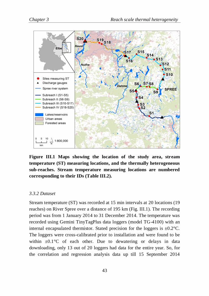
Figure III.1 Maps showing the location of the study area, stream
temperature (ST) measuring locations, and the thermally heterogeneous
sub-reaches. Stream temperature measuring locations are numbered
corresponding to their IDs (Table III.2).
3.3.2 Dataset
Stream temperature (ST) was recorded at 15 min intervals at 20 locations (19
reaches) on River Spree over a distance of 195 km (Fig. III.1). The recording
period was from 1 January 2014 to 31 December 2014. The temperature was
recorded using Gemini TinyTagPlus data loggers (model TG-4100) with an
internal encapsulated thermistor. Stated precision for the loggers is ±0.2°C.
The loggers were cross-calibrated prior to installation and were found to be
within ±0.1°C of each other. Due to dewatering or delays in data
downloading, only 13 out of 20 loggers had data for the entire year. So, for
the correlation and regression analysis data up till 15 September 2014
Chapter 3 Reach scale thermal heterogeneity
44
(available for all loggers) were used, whereas for model applications entire
year’s data were used where available.
Table III.1 Hydro-climatological and landscape variables considered in
the analysis.
Hydro-climatological
variables Landscape variables
Air temperature [°C] Forest area in 50 m buffer (F_50) [%]
Solar radiation [J cm-2
] Forest area in 100 m buffer (F_100) [%]
Relative humidity [%] Forest area in 500 m buffer (F_500) [%]
Wind velocity [m s-1
] Forest area in 1000 m buffer (F_1000) [%]
Atmospheric pressure [mbar] Agricultural area in 50 m buffer (F_50) [%]
Cloud cover [okta] Agricultural area in 100 m buffer (F_100) [%]
Discharge [m s-3
] Agricultural area in 500 m buffer (F_500) [%]
Agricultural in 1000 m buffer (F_1000) [%]
Urban area in 50 m buffer (F_50) [%]
Urban area in 100 m buffer (F_100) [%]
Urban area in 500 m buffer (F_500) [%]
Urban area in 1000 m buffer (F_1000) [%]
Lake distance [m]
Stream azimuth (aspect) [°]
Hourly data for climatological variables such as air temperature, relative
humidity, wind velocity, atmospheric pressure, cloud cover and shortwave
radiation were downloaded from the Deutsche Wetter Dienst (DWD,
www.dwd.de) for the relevant period. This data were available at five
locations for air temperature and relative humidity whereas only at a single
location for the rest of the variables. Therefore, the data of the five stations
were averaged across sites for each time step to obtain the air temperature
and relative humidity data for the region. Daily discharge (flow) data were
obtained from Landesamt für Umwelt, Gesundheit und Verbraucherschutz
Chapter 3 Reach scale thermal heterogeneity
45
(LUGV; www.luis.brandenburg.de/) and were available at six locations
within the study reach (Fig. III.1).
A total of 14 landscape variables were included in the study and basically
comprised of shares (%) of land cover for different buffer widths, lake
distance and stream azimuth (aspect) (Table III.1; Fig. SIII.1). Land cover
data along the reach were obtained from ATKIS land-use dataset (10 m × 10
m resolution; ADV, Germany). Lake distances and stream azimuth values
were calculated from Google Earth. Azimuth was measured as the angle
(degrees) that the overall stream channel differed from due south (e.g., due
south = 0°, due west = +90°, and due east = -90°) (Arscott et al., 2001).
Since elevation was very similar across sites (58-30 m), it was not
considered for analysis.
3.3.3 Quantification of contribution of landscape controls in the heat budget
Heat content variations in a river reach was computed using the following
energy balance:
𝑑
𝑑𝑡(𝜌 𝐶𝑝 𝑉 𝑇𝑤) = 𝐻𝑢𝑝 − 𝐻𝑑𝑜𝑤𝑛 + 𝑆 (𝐸𝑎𝑡𝑚 + 𝐸𝑟 + ∆𝐸) (1)
where 𝑇𝑤 is stream temperature, 𝜌 and 𝐶𝑝 are density (assumed constant, 997
kg m-3
) and specific heat of water (assumed constant, 4179 J kg-1
°C-1
), 𝑉 is
volume of the reach (m3), 𝑆 is the surface area (m
2), 𝐻𝑢𝑝 is the total heat flux
entering (W) the volume from the upstream section, 𝐻𝑑𝑜𝑤𝑛 is the total heat
flux (W) going out downstream, 𝐸atm is the net exchange per unit surface (W
m-2
) with atmosphere estimated as an average value for the whole study area.
The various heat flux components of 𝐸atm (solar radiation, sensible and
latent heat flux, evaporation, condensation, etc.) were calculated using the
relationships reported in Martin & McCutcheon (1998) (see Appendix C).
The value ∆𝐸 is a correction factor (W m-2
) accounting for global
uncertainties in the determination of 𝐸𝑎𝑡𝑚 with the empirical heat budget
equations. Moreover, 𝐸𝑟 is the remaining energy flux term (W m-2
) that is
expected to be a contribution of sources other than the exchange with the
atmosphere, rescaled with the surface area 𝑆. This term is site-specific and is
assumed to majorly include the unresolved terms, such as land use- based
sources (such as wastewater, urban outflows), inflows from lakes, tributaries
and groundwater not explicitly included in 𝐻𝑢𝑝. Since the solar radiation
Chapter 3 Reach scale thermal heterogeneity
46
values were region-based and not site-based, effects of reduced incident solar
radiation (reduced heat inputs) in shaded areas are also included in 𝐸𝑟.
Equation (1) was discretized by subdividing the entire reach into
computational reaches defined by the location of the ST measuring sites.
Each computational reach had a discrete stream temperature 𝑇𝑤,𝑖𝑘 (°C, with 𝑖
the index for space and 𝑘 for time) in the volume 𝑉𝑖 . Assuming steady and
uniform hydraulic conditions (i.e., constant discharge, Q (m3 s
-1), or/and
cross-section) along a computational reach 𝑖, and further assuming that the
downstream temperature 𝑇𝑤,𝑑𝑜𝑤𝑛 ≅ 𝑇𝑤,𝑖𝑘 (thus considering each
computational reach as a completely mixed reactor), the upstream and
downstream heat fluxes were calculated as 𝐻𝑢𝑝 = 𝜌𝐶𝑝𝑄𝑖𝑇𝑤,𝑖−1 and 𝐻𝑑𝑜𝑤𝑛 =
𝜌𝐶𝑝𝑄𝑖𝑇𝑤,𝑖, respectively. Thus, the temperature change in a river reach can be
calculated by the following heat balance:
𝑇𝑤,𝑖
𝑘+1−𝑇𝑤,𝑖𝑘
∆𝑡=
𝑄𝑖
𝑉𝑖 (𝑇𝑤,𝑖−1
𝑘 − 𝑇𝑤,𝑖𝑘 ) + 𝑆𝑖
𝐸𝑎𝑡𝑚+ ∆𝐸
𝜌 𝐶𝑝 𝑉𝑖+ 𝑆𝑖
𝐸𝑟,𝑖
𝜌 𝐶𝑝 𝑉𝑖 , (2)
where, an explicit Euler scheme was used for the discretization, as a first
approximation. The volume was estimated as 𝑉𝑖 = 𝐵𝑖𝐷𝑖𝐿𝑖, where 𝐵𝑖 is the
river width (m), 𝐷𝑖 is the depth (m) and 𝐿𝑖 the length (m) of the reach. All
the surface heat fluxes were calculated referring to a surface area 𝑆𝑖 = 𝐵𝑖𝐿𝑖.
Alternatively, if the temperature changes across space and time are
known, equation (2) yields a way to estimate the residual heat term,
𝐸𝑟,𝑖 = 𝜌 𝐶𝑝 𝐷𝑖 (𝑇𝑤,𝑖
𝑘+1−𝑇𝑤,𝑖𝑘
∆𝑡) − 𝜌 𝐶𝑝
𝑄𝑖
𝐵𝑖𝐿𝑖 (𝑇𝑤,𝑖−1
𝑘 − 𝑇𝑤,𝑖𝑘 ) − 𝐸𝑎𝑡𝑚 − ∆𝐸 (3)
Some assumptions helped us in the interpretation of the residual term 𝐸𝑟 (W
m-2
). Groundwater contributions to ST spatial heterogeneity was assumed to
be negligible because water conductivity, an indicator of groundwater
inflow (Johnson and Wilby, 2015), was similar at most of the sites (Table
III.2). Regarding the influence of tributaries, although there are several small
streams or canals flowing into River Spree, not enough information on these
inputs was available. Also, there are no major tributaries joining directly
with the main river along the study reach, except River Dahme which joins
River Spree in its final reach. Hence, tributary contributions were also
Chapter 3 Reach scale thermal heterogeneity
47
assumed to be negligible. Ultimately, 𝐸𝑟 mainly consists of heat
contributions from land-use sources and lake inflows (the latter by means of
alterations of the upstream heat flux) within the reach.
For this analysis, the 19 sections in River Spree were analysed in six groups
(S1 to S2; S3 to S5; S6 to S9; S10 to S14; S15 to S17; S18 to S20; see Fig
III.1) according to the discharge information available. The discharge in each
group was assumed to be constant. The calculations were performed using
daily averaged values of ST and hydro-climatological variables.
Chapter 3 Reach scale thermal heterogeneity
48
Table III.2 Description of the stream temperature observation sites on River Spree.
Thermally
different
sub-
reaches
Site
ID
Name Distance
(km)
Mean
ST for
entire
period
Maximum
ST
(15 min)
Time at
Maximum
ST
Forest
Area
(% of
total in
reach;
50 m
wide
buffer)
Urban
Area
(% of
total in
reach; 50
m wide
buffer)
Distance
from the
closest
lake
(km)
Conductivit
y
(μ cm-1
;
daily mean
value on
14 Jan
2008)
Sub-reach
I
S1 Leipe 0 13.04 24.25 21-07 17:15 30 16 51 947
S2 Lubben 14 13.06 24.87 21-07 17:30 62 17 65 857
S3 Hartmannsdorf 18 13.14 25.26 21-07 17:00 32 50 69 822
S4 Schlepzig 27 13.25 25.30 22-07 18:00 92 2 78 NA
S5 Leibsch 33 13.32 25.26 22-07 18:15 33 5 84 815
Sub-reach
II
S6 Altschadow 42 13.95 27.78 20-07 15:00 13 10 0.5 893
S7 Werder 49 13.90 26.83 21-07 02:15 19 1 8 NA
S8 Kosenblatt 52 13.73 27.08 21-07 15:00 23 6 11 NA
S9 Trebatsch 62 13.77 26.37 21-07 23:15 22 7 21 0.88
Sub-reach
III
S10 Radinkendorf 81 14.13 26.88 21-07 16:15 41 13 2 823
S11 Rassmansdorf 87 14.03 26.41 21-07 16:30 25 2 8 0.84
S12 Drahendorf 99 13.80 25.77 20-07 16:15 35 3 10 837
S13 Berkenbrucke 108 13.84 26.59 22-07 11:30 52 5 19 NA
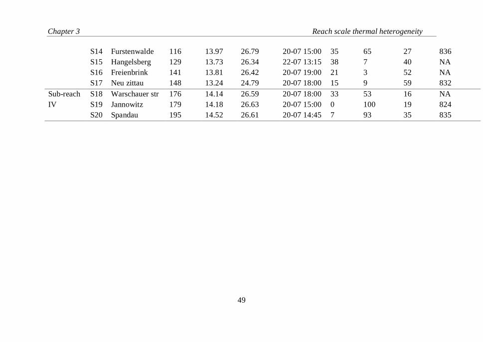
Chapter 3 Reach scale thermal heterogeneity
49
S14 Furstenwalde 116 13.97 26.79 20-07 15:00 35 65 27 836
S15 Hangelsberg 129 13.73 26.34 22-07 13:15 38 7 40 NA
S16 Freienbrink 141 13.81 26.42 20-07 19:00 21 3 52 NA
S17 Neu zittau 148 13.24 24.79 20-07 18:00 15 9 59 832
Sub-reach
IV
S18 Warschauer str 176 14.14 26.59 20-07 18:00 33 53 16 NA
S19 Jannowitz 179 14.18 26.63 20-07 15:00 0 100 19 824
S20 Spandau 195 14.52 26.61 20-07 14:45 7 93 35 835
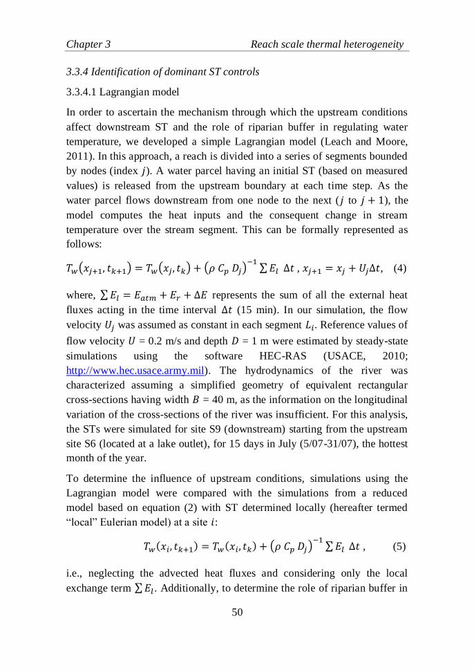
Chapter 3 Reach scale thermal heterogeneity
50
3.3.4 Identification of dominant ST controls
3.3.4.1 Lagrangian model
In order to ascertain the mechanism through which the upstream conditions
affect downstream ST and the role of riparian buffer in regulating water
temperature, we developed a simple Lagrangian model (Leach and Moore,
2011). In this approach, a reach is divided into a series of segments bounded
by nodes (index 𝑗). A water parcel having an initial ST (based on measured
values) is released from the upstream boundary at each time step. As the
water parcel flows downstream from one node to the next (𝑗 to 𝑗 + 1), the
model computes the heat inputs and the consequent change in stream
temperature over the stream segment. This can be formally represented as
follows:
𝑇𝑤(𝑥𝑗+1, 𝑡𝑘+1) = 𝑇𝑤(𝑥𝑗, 𝑡𝑘) + (𝜌 𝐶𝑝 𝐷𝑗)−1
∑ 𝐸𝑙 ∆𝑡 , 𝑥𝑗+1 = 𝑥𝑗 + 𝑈𝑗∆𝑡, (4)
where, ∑ 𝐸𝑙 = 𝐸𝑎𝑡𝑚 + 𝐸𝑟 + ∆𝐸 represents the sum of all the external heat
fluxes acting in the time interval ∆𝑡 (15 min). In our simulation, the flow
velocity 𝑈𝑗 was assumed as constant in each segment 𝐿𝑖. Reference values of
flow velocity 𝑈 = 0.2 m/s and depth 𝐷 = 1 m were estimated by steady-state
simulations using the software HEC-RAS (USACE, 2010;
http://www.hec.usace.army.mil). The hydrodynamics of the river was
characterized assuming a simplified geometry of equivalent rectangular
cross-sections having width 𝐵 = 40 m, as the information on the longitudinal
variation of the cross-sections of the river was insufficient. For this analysis,
the STs were simulated for site S9 (downstream) starting from the upstream
site S6 (located at a lake outlet), for 15 days in July (5/07-31/07), the hottest
month of the year.
To determine the influence of upstream conditions, simulations using the
Lagrangian model were compared with the simulations from a reduced
model based on equation (2) with ST determined locally (hereafter termed
“local” Eulerian model) at a site 𝑖:
𝑇𝑤(𝑥𝑖, 𝑡𝑘+1) = 𝑇𝑤(𝑥𝑖, 𝑡𝑘) + (𝜌 𝐶𝑝 𝐷𝑗)−1
∑ 𝐸𝑙 ∆𝑡 , (5)
i.e., neglecting the advected heat fluxes and considering only the local
exchange term ∑ 𝐸𝑙 . Additionally, to determine the role of riparian buffer in
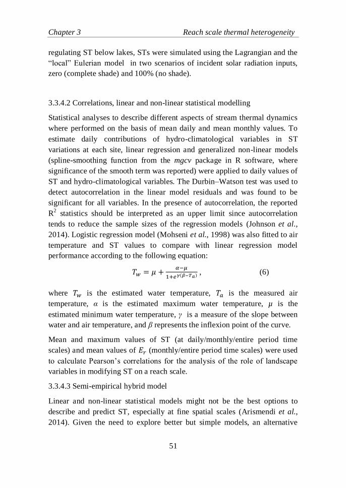
Chapter 3 Reach scale thermal heterogeneity
51
regulating ST below lakes, STs were simulated using the Lagrangian and the
“local” Eulerian model in two scenarios of incident solar radiation inputs,
zero (complete shade) and 100% (no shade).
3.3.4.2 Correlations, linear and non-linear statistical modelling
Statistical analyses to describe different aspects of stream thermal dynamics
where performed on the basis of mean daily and mean monthly values. To
estimate daily contributions of hydro-climatological variables in ST
variations at each site, linear regression and generalized non-linear models
(spline-smoothing function from the mgcv package in R software, where
significance of the smooth term was reported) were applied to daily values of
ST and hydro-climatological variables. The Durbin–Watson test was used to
detect autocorrelation in the linear model residuals and was found to be
significant for all variables. In the presence of autocorrelation, the reported
R2 statistics should be interpreted as an upper limit since autocorrelation
tends to reduce the sample sizes of the regression models (Johnson et al.,
2014). Logistic regression model (Mohseni et al., 1998) was also fitted to air
temperature and ST values to compare with linear regression model
performance according to the following equation:
𝑇𝑤 = 𝜇 +𝛼−𝜇
1+𝑒𝛾(𝛽−𝑇𝑎) , (6)
where 𝑇𝑤 is the estimated water temperature, 𝑇𝑎 is the measured air
temperature, α is the estimated maximum water temperature, µ is the
estimated minimum water temperature, γ is a measure of the slope between
water and air temperature, and β represents the inflexion point of the curve.
Mean and maximum values of ST (at daily/monthly/entire period time
scales) and mean values of 𝐸𝑟 (monthly/entire period time scales) were used
to calculate Pearson’s correlations for the analysis of the role of landscape
variables in modifying ST on a reach scale.
3.3.4.3 Semi-empirical hybrid model
Linear and non-linear statistical models might not be the best options to
describe and predict ST, especially at fine spatial scales (Arismendi et al.,
2014). Given the need to explore better but simple models, an alternative
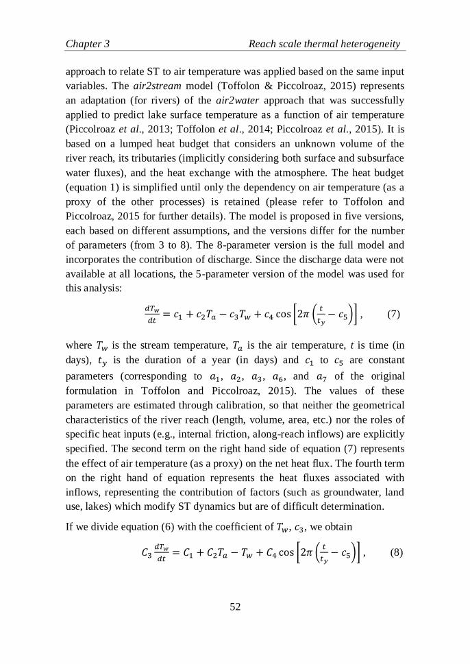
Chapter 3 Reach scale thermal heterogeneity
52
approach to relate ST to air temperature was applied based on the same input
variables. The air2stream model (Toffolon & Piccolroaz, 2015) represents
an adaptation (for rivers) of the air2water approach that was successfully
applied to predict lake surface temperature as a function of air temperature
(Piccolroaz et al., 2013; Toffolon et al., 2014; Piccolroaz et al., 2015). It is
based on a lumped heat budget that considers an unknown volume of the
river reach, its tributaries (implicitly considering both surface and subsurface
water fluxes), and the heat exchange with the atmosphere. The heat budget
(equation 1) is simplified until only the dependency on air temperature (as a
proxy of the other processes) is retained (please refer to Toffolon and
Piccolroaz, 2015 for further details). The model is proposed in five versions,
each based on different assumptions, and the versions differ for the number
of parameters (from 3 to 8). The 8-parameter version is the full model and
incorporates the contribution of discharge. Since the discharge data were not
available at all locations, the 5-parameter version of the model was used for
this analysis:
𝑑𝑇𝑤
𝑑𝑡= 𝑐1 + 𝑐2𝑇𝑎 − 𝑐3𝑇𝑤 + 𝑐4 cos [2𝜋 (
𝑡
𝑡𝑦− 𝑐5)] , (7)
where 𝑇𝑤 is the stream temperature, 𝑇𝑎 is the air temperature, t is time (in
days), 𝑡𝑦 is the duration of a year (in days) and 𝑐1 to 𝑐5 are constant
parameters (corresponding to 𝑎1, 𝑎2, 𝑎3, 𝑎6, and 𝑎7 of the original
formulation in Toffolon and Piccolroaz, 2015). The values of these
parameters are estimated through calibration, so that neither the geometrical
characteristics of the river reach (length, volume, area, etc.) nor the roles of
specific heat inputs (e.g., internal friction, along-reach inflows) are explicitly
specified. The second term on the right hand side of equation (7) represents
the effect of air temperature (as a proxy) on the net heat flux. The fourth term
on the right hand of equation represents the heat fluxes associated with
inflows, representing the contribution of factors (such as groundwater, land
use, lakes) which modify ST dynamics but are of difficult determination.
If we divide equation (6) with the coefficient of 𝑇𝑤, 𝑐3, we obtain
𝐶3𝑑𝑇𝑤
𝑑𝑡= 𝐶1 + 𝐶2𝑇𝑎 − 𝑇𝑤 + 𝐶4 cos [2𝜋 (
𝑡
𝑡𝑦− 𝑐5)] , (8)
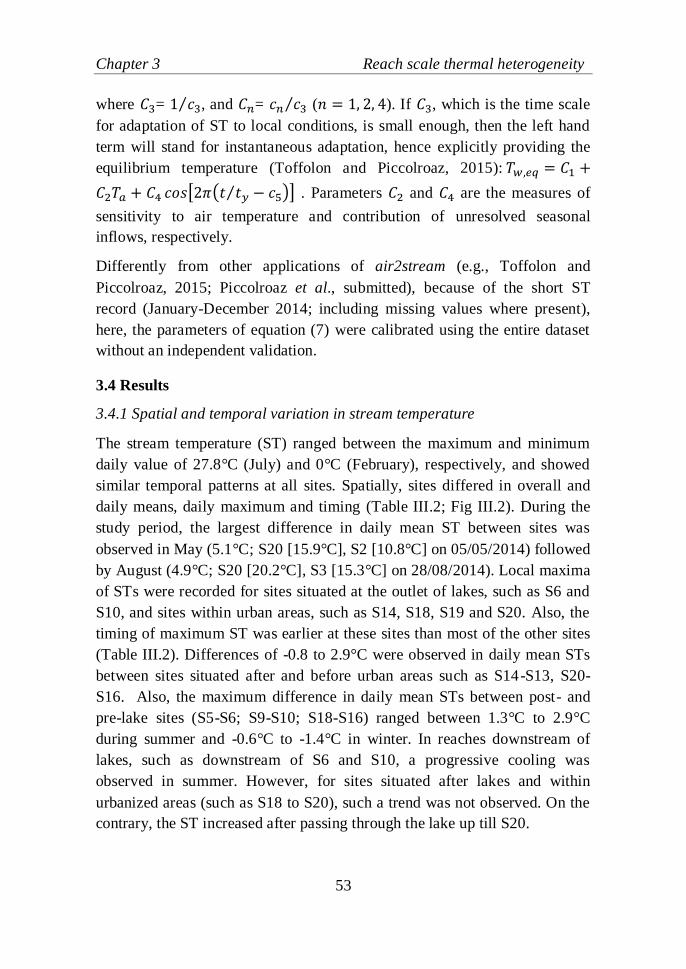
Chapter 3 Reach scale thermal heterogeneity
53
where 𝐶3= 1 𝑐3⁄ , and 𝐶𝑛= 𝑐𝑛 𝑐3⁄ (𝑛 = 1, 2, 4). If 𝐶3, which is the time scale
for adaptation of ST to local conditions, is small enough, then the left hand
term will stand for instantaneous adaptation, hence explicitly providing the
equilibrium temperature (Toffolon and Piccolroaz, 2015): 𝑇𝑤,𝑒𝑞 = 𝐶1 +
𝐶2𝑇𝑎 + 𝐶4 𝑐𝑜𝑠[2𝜋(𝑡 𝑡𝑦⁄ − 𝑐5)] . Parameters 𝐶2 and 𝐶4 are the measures of
sensitivity to air temperature and contribution of unresolved seasonal
inflows, respectively.
Differently from other applications of air2stream (e.g., Toffolon and
Piccolroaz, 2015; Piccolroaz et al., submitted), because of the short ST
record (January-December 2014; including missing values where present),
here, the parameters of equation (7) were calibrated using the entire dataset
without an independent validation.
3.4 Results
3.4.1 Spatial and temporal variation in stream temperature
The stream temperature (ST) ranged between the maximum and minimum
daily value of 27.8°C (July) and 0°C (February), respectively, and showed
similar temporal patterns at all sites. Spatially, sites differed in overall and
daily means, daily maximum and timing (Table III.2; Fig III.2). During the
study period, the largest difference in daily mean ST between sites was
observed in May (5.1°C; S20 [15.9°C], S2 [10.8°C] on 05/05/2014) followed
by August (4.9°C; S20 [20.2°C], S3 [15.3°C] on 28/08/2014). Local maxima
of STs were recorded for sites situated at the outlet of lakes, such as S6 and
S10, and sites within urban areas, such as S14, S18, S19 and S20. Also, the
timing of maximum ST was earlier at these sites than most of the other sites
(Table III.2). Differences of -0.8 to 2.9°C were observed in daily mean STs
between sites situated after and before urban areas such as S14-S13, S20-
S16. Also, the maximum difference in daily mean STs between post- and
pre-lake sites (S5-S6; S9-S10; S18-S16) ranged between 1.3°C to 2.9°C
during summer and -0.6°C to -1.4°C in winter. In reaches downstream of
lakes, such as downstream of S6 and S10, a progressive cooling was
observed in summer. However, for sites situated after lakes and within
urbanized areas (such as S18 to S20), such a trend was not observed. On the
contrary, the ST increased after passing through the lake up till S20.
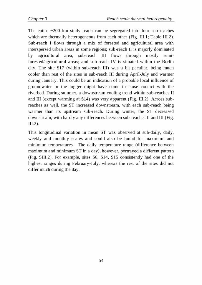
Chapter 3 Reach scale thermal heterogeneity
54
The entire ~200 km study reach can be segregated into four sub-reaches
which are thermally heterogeneous from each other (Fig. III.1; Table III.2).
Sub-reach I flows through a mix of forested and agricultural area with
interspersed urban areas in some regions; sub-reach II is majorly dominated
by agricultural area; sub-reach III flows through mostly semi-
forested/agricultural areas; and sub-reach IV is situated within the Berlin
city. The site S17 (within sub-reach III) was a bit peculiar, being much
cooler than rest of the sites in sub-reach III during April-July and warmer
during January. This could be an indication of a probable local influence of
groundwater or the logger might have come in close contact with the
riverbed. During summer, a downstream cooling trend within sub-reaches II
and III (except warming at S14) was very apparent (Fig. III.2). Across sub-
reaches as well, the ST increased downstream, with each sub-reach being
warmer than its upstream sub-reach. During winter, the ST decreased
downstream, with hardly any differences between sub-reaches II and III (Fig.
III.2).
This longitudinal variation in mean ST was observed at sub-daily, daily,
weekly and monthly scales and could also be found for maximum and
minimum temperatures. The daily temperature range (difference between
maximum and minimum ST in a day), however, portrayed a different pattern
(Fig. SIII.2). For example, sites S6, S14, S15 consistently had one of the
highest ranges during February-July, whereas the rest of the sites did not
differ much during the day.
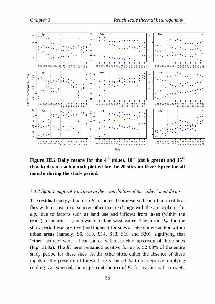
Chapter 3 Reach scale thermal heterogeneity
55
Figure III.2 Daily means for the 4th
(blue), 10th
(dark green) and 15th
(black) day of each month plotted for the 20 sites on River Spree for all
months during the study period.
3.4.2 Spatiotemporal variation in the contribution of the ‘other’ heat fluxes
The residual energy flux term 𝐸𝑟 denotes the unresolved contribution of heat
flux within a reach via sources other than exchange with the atmosphere, for
e.g., due to factors such as land use and inflows from lakes (within the
reach), tributaries, groundwater and/or wastewater. The mean 𝐸𝑟 for the
study period was positive (and highest) for sites at lake outlets and/or within
urban areas (namely, S6, S10, S14, S18, S19 and S20), signifying that
‘other’ sources were a heat source within reaches upstream of these sites
(Fig. III.3a). The 𝐸𝑟 term remained positive for up to 52-63% of the entire
study period for these sites. At the other sites, either the absence of these
inputs or the presence of forested areas caused 𝐸𝑟 to be negative, implying
cooling. As expected, the major contribution of 𝐸𝑟 for reaches with sites S6,
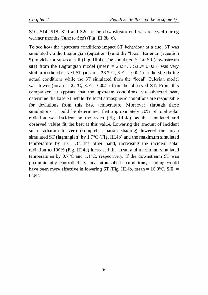
Chapter 3 Reach scale thermal heterogeneity
56
S10, S14, S18, S19 and S20 at the downstream end was received during
warmer months (June to Sep) (Fig. III.3b, c).
To see how the upstream conditions impact ST behaviour at a site, ST was
simulated via the Lagrangian (equation 4) and the “local” Eulerian (equation
5) models for sub-reach II (Fig. III.4). The simulated ST at S9 (downstream
site) from the Lagrangian model (mean = 23.5°C, S.E.= 0.023) was very
similar to the observed ST (mean = 23.7°C, S.E. = 0.021) at the site during
actual conditions while the ST simulated from the “local” Eulerian model
was lower (mean = 22°C, S.E.= 0.021) than the observed ST. From this
comparison, it appears that the upstream conditions, via advected heat,
determine the base ST while the local atmospheric conditions are responsible
for deviations from this base temperature. Moreover, through these
simulations it could be determined that approximately 70% of total solar
radiation was incident on the reach (Fig. III.4a), as the simulated and
observed values fit the best at this value. Lowering the amount of incident
solar radiation to zero (complete riparian shading) lowered the mean
simulated ST (lagrangian) by 1.7°C (Fig. III.4b) and the maximum simulated
temperature by 1°C. On the other hand, increasing the incident solar
radiation to 100% (Fig. III.4c) increased the mean and maximum simulated
temperatures by 0.7°C and 1.1°C, respectively. If the downstream ST was
predominantly controlled by local atmospheric conditions, shading would
have been more effective in lowering ST (Fig. III.4b, mean = 16.8°C, S.E. =
0.04).
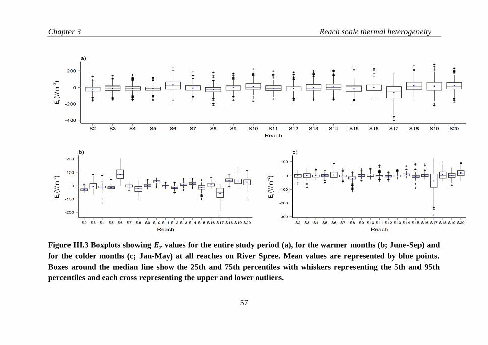
Chapter 3 Reach scale thermal heterogeneity
57
Figure III.3 Boxplots showing 𝑬𝒓 values for the entire study period (a), for the warmer months (b; June-Sep) and
for the colder months (c; Jan-May) at all reaches on River Spree. Mean values are represented by blue points.
Boxes around the median line show the 25th and 75th percentiles with whiskers representing the 5th and 95th
percentiles and each cross representing the upper and lower outliers.
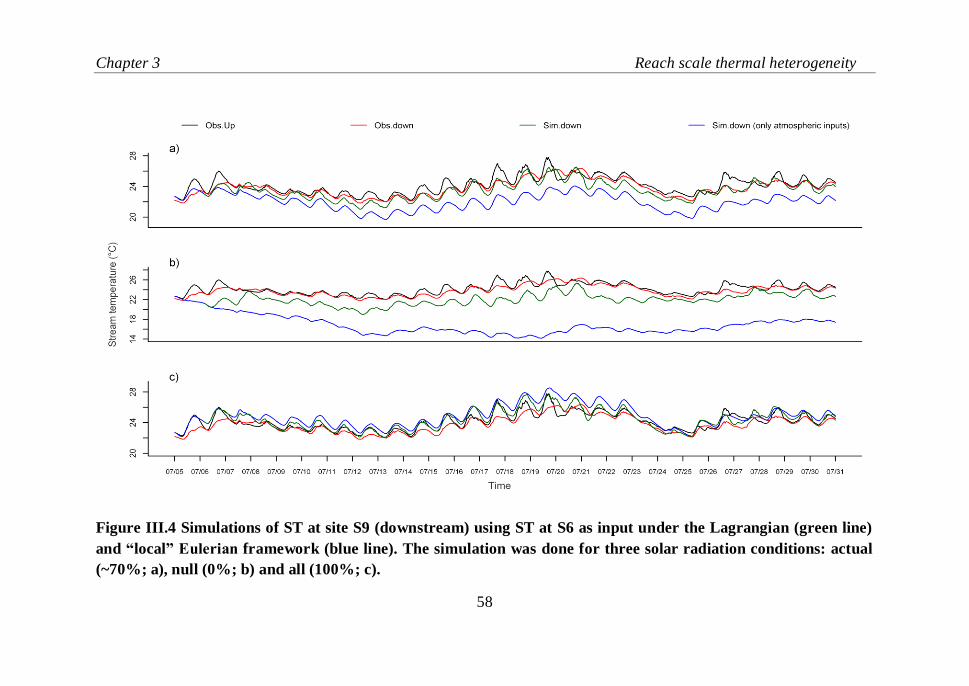
Chapter 3 Reach scale thermal heterogeneity
58
Figure III.4 Simulations of ST at site S9 (downstream) using ST at S6 as input under the Lagrangian (green line)
and “local” Eulerian framework (blue line). The simulation was done for three solar radiation conditions: actual
(~70%; a), null (0%; b) and all (100%; c).
Chapter 3 Reach scale thermal heterogeneity
59
3.4.3 Dependence on hydro-climatological and landscape variables
3.4.3.1 Correlations with hydro-climatological variables
Among the seven hydro-climatological variables considered, air temperature,
solar radiation and relative humidity were fairly linearly related with ST,
while the other variables shared a non-linear relationship (Fig. SIII.3, not
shown for discharge). Air temperature (82-88%) and solar radiation (54-
58%) explained the highest percentage of temporal ST variability for all sites
(Fig. III.5). Air temperature contributions decreased consistently from
upstream to downstream whereas that of solar radiation remained relatively
constant. Discharge, relative humidity and atmospheric pressure explained,
on average, 38% (standard error, S.E.= 0.03), 16% (S.E.= 0.001) and 15%
(S.E.= 0.002) of ST variability respectively (Fig. III.5). The effect of
discharge was the highest for upstream sites S3, S4 and S5, while the lowest
was for S2 and S3. Several small forested canals in the lower Spreewald
region and the bigger Nordumfluter canal flow into the main stem between
S2 and S3 and probably contribute to a larger portion of discharge. Hence,
the ST in this reach is largely a reflection of the water temperatures in the
canals. Other climatological variables contributed less significantly,
explaining < 10% of temporal ST variability. Together, the hydro-
climatological variables explained 89-92% (multiple regression) of the ST
variability.
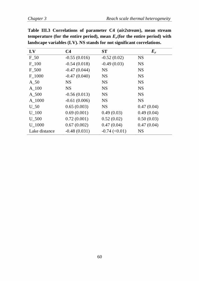
Chapter 3 Reach scale thermal heterogeneity
60
Table III.3 Correlations of parameter C4 (air2stream), mean stream
temperature (for the entire period), mean 𝑬𝒓(for the entire period) with
landscape variables (LV). NS stands for not significant correlations.
LV C4 ST 𝑬𝒓
F_50 -0.55 (0.016) -0.52 (0.02) NS
F_100 -0.54 (0.018) -0.49 (0.03) NS
F_500 -0.47 (0.044) NS NS
F_1000 -0.47 (0.040) NS NS
A_50 NS NS NS
A_100 NS NS NS
A_500 -0.56 (0.013) NS NS
A_1000 -0.61 (0.006) NS NS
U_50 0.65 (0.003) NS 0.47 (0.04)
U_100 0.69 (0.001) 0.49 (0.03) 0.49 (0.04)
U_500 0.72 (0.001) 0.52 (0.02) 0.50 (0.03)
U_1000 0.67 (0.002) 0.47 (0.04) 0.47 (0.04)
Lake distance -0.48 (0.031) -0.74 (<0.01) NS
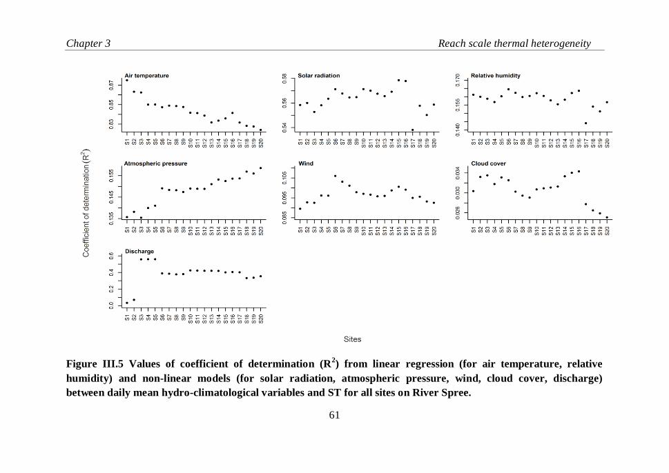
Chapter 3 Reach scale thermal heterogeneity
61
Figure III.5 Values of coefficient of determination (R2) from linear regression (for air temperature, relative
humidity) and non-linear models (for solar radiation, atmospheric pressure, wind, cloud cover, discharge)
between daily mean hydro-climatological variables and ST for all sites on River Spree.
Chapter 3 Reach scale thermal heterogeneity
62
3.4.3.2 Correlations with landscape variables
Stream temperature: Several significant correlations of ST metrics with
landscape variables were detected at monthly, daily scales as well as for the
entire time period. Over the study period, share (%) of urban and forest area
in >50 m and ≤100 m wide buffers, respectively, were significantly
correlated with the mean STs (Table III.3). At the monthly scale, significant
correlations of land use shares with mean STs were observed mostly for
warmer months (May-Sep) (Table III.4). Share of forest area within 100 m
had a significant negative correlation with both mean and maximum monthly
STs. On the other hand, share of urban area showed strong significant
correlations with mean monthly STs during warm months (positive) and with
maximum monthly STs during February (negative), irrespective of the buffer
width (Table III.4). Share of agricultural area was also significantly
correlated with mean monthly STs during warm months (≥500 m) and with
maximum monthly STs during February (all buffer widths). At the daily
scale, share of forest cover within 50 m and urban cover within 500 m had
the highest number of significant correlations with mean ST (44% of 259
days) as well as with maximum ST (forest (50 m): 38%; urban (500 m):
36%).
Distance from lakes had a significant negative correlation with the mean ST
for the study period (Table III.3). At the monthly scale, mean and maximum
STs of warmer months had a significant negative correlation with lake
distance, while a significant positive relationship was observed during the
coldest months (Table III.4). At the daily scale, significant correlations of
lake distance with mean and maximum STs were similar in number (mean =
73.7%; max = 72.2%). No significant correlations between stream azimuth
and ST were detected at any time scale.
Residual heat flux 𝐸𝑟: Mean 𝐸𝑟 for the study period was significantly
correlated with only the share of urban area irrespective of the buffer widths
(Table III.3). At the monthly scale, significant correlations of land use cover
with mean 𝐸𝑟 were also detected mostly for warmer months (Table III.5).
Share of forest cover in ≥500 m buffer widths were negatively correlated
with mean monthly 𝐸𝑟 while urban cover had significant positive
correlations for all buffer widths. There were no significant correlations with
agricultural cover.
Chapter 3 Reach scale thermal heterogeneity
63
Significant correlations of lake distance with mean monthly 𝐸𝑟 were
observed, but not with the mean for the entire study period (Tables III.3,
III.5). Lake distance had significant correlations with mean monthly 𝐸𝑟 in
February (positive) and in warmer months (June-Sep; negative correlation).
There were no significant correlations with stream azimuth.
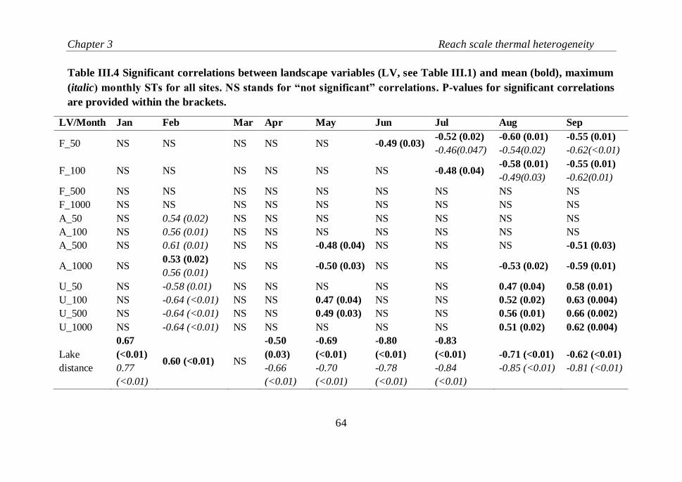
Chapter 3 Reach scale thermal heterogeneity
64
Table III.4 Significant correlations between landscape variables (LV, see Table III.1) and mean (bold), maximum
(italic) monthly STs for all sites. NS stands for “not significant” correlations. P-values for significant correlations
are provided within the brackets.
LV/Month Jan Feb Mar Apr May Jun Jul Aug Sep
F_50 NS NS NS NS NS -0.49 (0.03) -0.52 (0.02)
-0.46(0.047)
-0.60 (0.01)
-0.54(0.02)
-0.55 (0.01)
-0.62(<0.01)
F_100 NS NS NS NS NS NS -0.48 (0.04) -0.58 (0.01)
-0.49(0.03)
-0.55 (0.01)
-0.62(0.01)
F_500 NS NS NS NS NS NS NS NS NS
F_1000 NS NS NS NS NS NS NS NS NS
A_50 NS 0.54 (0.02) NS NS NS NS NS NS NS
A_100 NS 0.56 (0.01) NS NS NS NS NS NS NS
A_500 NS 0.61 (0.01) NS NS -0.48 (0.04) NS NS NS -0.51 (0.03)
A_1000 NS 0.53 (0.02)
0.56 (0.01) NS NS -0.50 (0.03) NS NS -0.53 (0.02) -0.59 (0.01)
U_50 NS -0.58 (0.01) NS NS NS NS NS 0.47 (0.04) 0.58 (0.01)
U_100 NS -0.64 (<0.01) NS NS 0.47 (0.04) NS NS 0.52 (0.02) 0.63 (0.004)
U_500 NS -0.64 (<0.01) NS NS 0.49 (0.03) NS NS 0.56 (0.01) 0.66 (0.002)
U_1000 NS -0.64 (<0.01) NS NS NS NS NS 0.51 (0.02) 0.62 (0.004)
Lake
distance
0.67
(<0.01)
0.77
(<0.01)
0.60 (<0.01) NS
-0.50
(0.03)
-0.66
(<0.01)
-0.69
(<0.01)
-0.70
(<0.01)
-0.80
(<0.01)
-0.78
(<0.01)
-0.83
(<0.01)
-0.84
(<0.01)
-0.71 (<0.01)
-0.85 (<0.01)
-0.62 (<0.01)
-0.81 (<0.01)
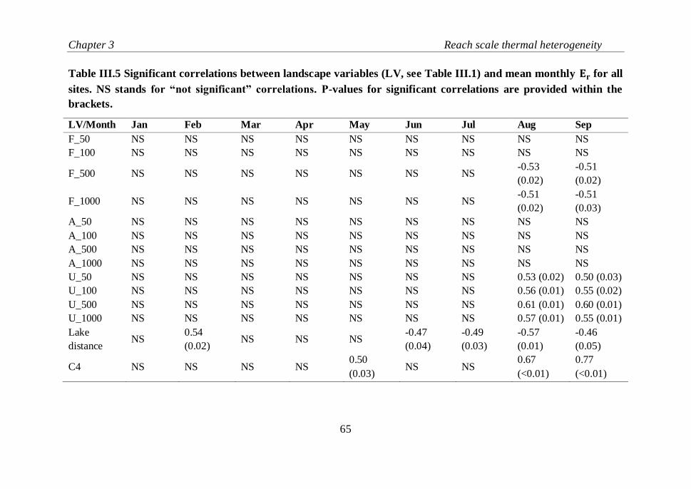
Chapter 3 Reach scale thermal heterogeneity
65
Table III.5 Significant correlations between landscape variables (LV, see Table III.1) and mean monthly 𝐄𝐫 for all
sites. NS stands for “not significant” correlations. P-values for significant correlations are provided within the
brackets.
LV/Month Jan Feb Mar Apr May Jun Jul Aug Sep
F_50 NS NS NS NS NS NS NS NS NS
F_100 NS NS NS NS NS NS NS NS NS
F_500 NS NS NS NS NS NS NS -0.53
(0.02)
-0.51
(0.02)
F_1000 NS NS NS NS NS NS NS -0.51
(0.02)
-0.51
(0.03)
A_50 NS NS NS NS NS NS NS NS NS
A_100 NS NS NS NS NS NS NS NS NS
A_500 NS NS NS NS NS NS NS NS NS
A_1000 NS NS NS NS NS NS NS NS NS
U_50 NS NS NS NS NS NS NS 0.53 (0.02) 0.50 (0.03)
U_100 NS NS NS NS NS NS NS 0.56 (0.01) 0.55 (0.02)
U_500 NS NS NS NS NS NS NS 0.61 (0.01) 0.60 (0.01)
U_1000 NS NS NS NS NS NS NS 0.57 (0.01) 0.55 (0.01)
Lake
distance NS
0.54
(0.02) NS NS NS
-0.47
(0.04)
-0.49
(0.03)
-0.57
(0.01)
-0.46
(0.05)
C4 NS NS NS NS 0.50
(0.03) NS NS
0.67
(<0.01)
0.77
(<0.01)
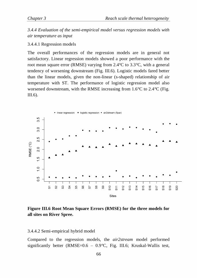
Chapter 3 Reach scale thermal heterogeneity
66
3.4.4 Evaluation of the semi-empirical model versus regression models with
air temperature as input
3.4.4.1 Regression models
The overall performances of the regression models are in general not
satisfactory. Linear regression models showed a poor performance with the
root mean square error (RMSE) varying from 2.4°C to 3.3°C, with a general
tendency of worsening downstream (Fig. III.6). Logistic models fared better
than the linear models, given the non-linear (s-shaped) relationship of air
temperature with ST. The performance of logistic regression model also
worsened downstream, with the RMSE increasing from 1.6°C to 2.4°C (Fig.
III.6).
Figure III.6 Root Mean Square Errors (RMSE) for the three models for
all sites on River Spree.
3.4.4.2 Semi-empirical hybrid model
Compared to the regression models, the air2stream model performed
significantly better (RMSE=0.6 – 0.9°C, Fig. III.6; Kruskal-Wallis test,
Chapter 3 Reach scale thermal heterogeneity
67
P<0.001). Similar to regression models, the RMSE showed a slight
increasing trend in the downstream direction of the reach. Being a hybrid
model, the parameters of air2stream can be analysed to better understand the
dynamics governing the thermal response of the river. The parameter 𝑐3 in
equation (7) represents the inverse of the temporal scale of the thermal
response to external forcing (Toffolon and Piccolroaz, 2015). The values of
this time scale (𝐶3 = 𝑐3−1), which ranged from 2.3 (S1) to 6.7 days (S18),
increased from upstream to downstream till S18 and then decreased for the
last two sites (Fig. III.7). This suggests that the thermal inertia of the reach
increases downstream, implying a greater effect of upstream conditions,
thereby increasing the theoretical time taken to reach equilibrium with the
local air temperature.
Although the equilibrium version of the model cannot be used because of the
relatively long adaptation time 𝐶3, the ratios defined in equation (8) are
calculated because they allow for a simpler interpretation than the coefficient
of equation (7). Their spatial variation is shown in Fig. III.7. The parameter
𝐶4, which represents the approximate contribution of factors different from
air temperature (such as land-use, lake or tributary inputs) to ST dynamics,
varied between 2.3 to 5°C. The largest values were estimated for the last
three sites in the study reach (S18-S20, Fig. III.7), suggesting that the
contribution of the unresolved fluxes was the highest in the city. Parameter
𝐶4 had strong significant correlations with all the land-use variables (Table
III.3), except share of agricultural area in ≤100 m buffers. It was positively
correlated with the share of urban cover, whereas negatively correlated with
agricultural cover, forest cover and lake distance. The overall mean heat flux
𝐸𝑟 was positively related with parameter 𝐶4 (significant; r = 0.57; P = 0.01),
confirming that both terms quantify the contribution of ‘other’ sources to ST.
On a monthly basis, 𝐸𝑟 and 𝐶4 had strong and significant positive
correlations for the warmer months (May, Aug, Sep) (Table III.5). The
parameter 𝐶1, which incorporates the annual constant flux in the model,
varied between 3 to 6.2°C, being the highest again for the last three sites
(S18-S20, Fig. III.7). The parameter 𝐶2, the coefficient associated with air
temperature, varied less than the other parameters (0.6 to 0.8) and was the
lowest for site S20 (Fig. III.7).
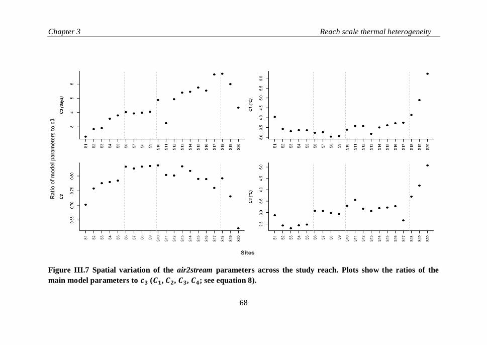
Chapter 3 Reach scale thermal heterogeneity
68
Figure III.7 Spatial variation of the air2stream parameters across the study reach. Plots show the ratios of the
main model parameters to 𝒄𝟑 (𝑪𝟏, 𝑪𝟐, 𝑪𝟑, 𝑪𝟒; see equation 8).
Chapter 3 Reach scale thermal heterogeneity
69
3.5 Discussion
3.5.1 Longitudinal heterogeneity in ST and its quantification in the heat
budget
Along the 200 km reach, the ST showed similar temporal patterns over the
study period at all sites in general. The inter-site differences mainly lay in the
timing of daily maximum ST and the magnitude of mean and maximum ST,
which were present at almost all time scales. In general, the STs warmed
from upstream to downstream in summer, whereas cooled in this direction in
winter. Although ST is generally observed to increase with increasing river
order (i.e. downstream) (Caissie, 2006), here it is also probable that this was
due to the presence of a large reservoir above the study reach, which
provided a water temperature that was lower than the equilibrium water
temperature in the river.
Based on the observed daily mean ST, the entire reach segregated in four
thermally different sub-reaches in warmer months and three sub-reaches in
colder months. Presence of lakes and/or presence of urbanized areas rather
than the presence/absence of forested areas marked these distinctions. The
influence of forested areas on ST is generally known to be more pronounced
in smaller streams than in larger streams, where increased stream width
prevents complete stream shading and reduces the impact of riparian forest
microclimates on the stream energy budget (Hannah et al., 2008; Hrachowitz
et al. 2010). Passage of river water through lakes and urban areas altered ST,
mostly during warmer months, as signified by the larger and mostly positive
residual heat flux term, 𝐸𝑟, during summer for reaches containing lakes or
cities. During winter, 𝐸𝑟 values were quite similar across sites, inferring no
significant influence of land use or lakes. Presence of urban areas resulted in
ST differences of up to 3°C. Cities tend to create urban heat islands, as air
and ground temperature within cities tend to be higher than the rural
surroundings (Pickett et al., 2001). Rivers flowing through such heat islands,
therefore, also tend to be warmer than rural and forested (Somers et al.,
2013). Several other studies have reported similar or larger differences (up to
8°C) between urban and non-urban areas (Pluhowski, 1970; Somers et al.,
2013; Booth et al. 2014). Pre- and post-lake STs also differed by -1 to 3°C in
the examined cases, an observation also made in other studies (Pedersen and
Sand-Jensen, 2007; Booth et al., 2014). Mostly, a progressive cooling was
Chapter 3 Reach scale thermal heterogeneity
70
observed in sub-reaches downstream of larger lakes in summer, while
temperatures remained similar in colder months. Lentic structures such as
lakes, ponds and wetlands have been seen to cause a delayed response in ST,
resulting in downstream cooling (late summer) and warming (spring) over
considerable distances (>100 m) (Mellina et al., 2002; Moore et al., 2005;
Booth et al., 2014). On the contrary, passage of lake outflows through urban
areas showed warming (in summer) as additional heat inputs from urban
areas into the river or a higher equilibrium temperature in that region might
have prevented heat loss from the reach.
3.5.2 Role of hydro-climatological and landscape variables in inducing
longitudinal ST heterogeneity
3.5.2.1 Hydro-climatological variables
Although the temporal variability of STs was largely explained by the usual
hydro-climatological variables (such as air temperature, solar radiation,
discharge), the contributions of these variables (especially air temperature)
decreased downstream of the reach, implying increasing contribution of
upstream conditions and/or other sources. Results from the application of the
air2stream and Lagrangian models corroborated this observation. Lagrangian
simulations suggest that the upstream conditions determined the base ST in
the study reach, while the climatic variability caused deviations around the
base ST. Also, parameter 𝐶4 from the air2stream model, which defines the
sensitivity of ST to ‘other’ sources such as landscape variables, showed a
general increasing trend, being the highest within urban areas or for sub-
reaches with lake inputs.
Values of sensitivity of ST to air temperature (described by the ratio 𝐶2 ≥0.6;
Fig. III.7), in the reach was typical of that of large rivers (stream order ≥ 4)
(Kelleher et al., 2012). In general, it is expected that ST sensitivity to air
temperatures would increase with increasing distance downstream, as it is a
function of river size and, hence, of the heat accumulated through the system
(Kelleher et al., 2012). However, this trend was seen only in the first 40 km
of the study reach, after which the sensitivity either remained constant or
decreased, again implying the role of other sources. Both local controls, such
as site characteristics, and non-local controls, such as cumulative influence of
the upstream network, quantify the magnitude of sensitivity. The sensitivity
was the highest for sites situated immediately downstream of lakes (S6, S10).
Chapter 3 Reach scale thermal heterogeneity
71
Shallow lakes, such as those found in the study area, present a greater surface
area and a longer residence time (as compared to rivers) for receiving solar
radiation and sensible heat exchange, thereby more effectively reaching
equilibrium with the local atmospheric conditions. Also, water temperatures
at lake outlets are probably more influenced by lakeshore water temperatures,
which are typically shallower. Sensitivity of ST to air temperature at site S18,
which is also below a lake, was not as high as that at the other lake-
influenced sites. This is probably because the lake before S18 (lake
Müggelsee) is deeper (max. depth = 8 m) than the other lakes (max. depth = 3
m).
3.5.2.2 Landscape variables
Significant correlations with the shares of land cover with spatial ST and 𝐸𝑟
variability across sites at different time scales (entire period/monthly/daily)
complement the modelling results. The share of urban area (irrespective of
the extent; across time scales) and lake distance (mostly at monthly scale)
was most consistently related with the spatial variability in ST and 𝐸𝑟. Lower
shares of urban cover and greater distance from lakes lead to lower heat
inputs during summers and, therefore, lowering ST. These results also
suggest that effect of urban areas was not dependent on its proximity to the
river, at least when situated within 1 km buffer. In another study, where the
local and watershed controls on summer ST were investigated (Booth et al.,
2014), local land cover was found to have greater influence on ST while the
effect of watershed urbanization was imperceptible. The other important ST
controls identified were upstream lakes and watershed geology.
Although forest area did seem to have a significant influence on reducing
heat inputs and moderating ST (negatively related to spatial ST and
𝐸𝑟 variability during summer), the effective extent buffer width was not clear.
With ST, share of forest area within 50 m were significantly related, while
with 𝐸𝑟, share of forest area in buffer widths ≥500 m had a significant
influence. Hrachowitz et al. (2012) also investigated the effectiveness of
riparian buffers and attained inconclusive results regarding effective extent,
suggesting a dynamic influence of extent of riparian buffers depending on
other site-based characteristics such as orientation, discharge, and
morphology. Regarding the effectiveness of the longitudinal extent of
riparian buffers in lake influenced reaches, presence of complete shading or
Chapter 3 Reach scale thermal heterogeneity
72
no shading (up to 20 km) caused a minor change in mean ST and
reduced/increased maximum ST by 1°C. This suggests that riparian buffers
might not be the best option, or should not be the only one, for regulating ST
in the region. Also, the influence of lakes plays a major role in the
determining downstream ST and seems to persist over substantial distances.
Spatial variation in land cover variables was related with spatial variability in
both daily mean and maximum ST, however, there were more instances of
significant correlations with daily mean ST. Although not conclusive, this
might suggest a greater influence of land cover on mean rather maximum ST.
In contrast, some other studies (Broadmeadow et al., 2011; Imholt et al.,
2013) suggest that land cover, such as forest area, influences maximum ST
more. Riparian buffers in the study reach are mostly patchy and, when
present, do not shade the river completely, thereby not directly and
effectively regulating maximum ST. With respect to urban areas, generally,
one of the major pathways through which they effect maximum ST is via
contribution of urban runoff (Booth et al., 2014). Considering that this region
is one of the driest areas in Germany, it is probable that contribution of urban
runoff to maximum ST is not frequent and the average temperatures are being
affected via other pathways, consistently occurring on a daily basis.
3.5.3 Beyond regression models
The weak performance of the regression models, especially linear regression,
at the daily scale, raises a question regarding their widespread applicability.
Generally, air and stream temperature correlations are typically weak at a
daily time scale and linear regressions are only accurate at moderate air
temperatures (0 to 20°C) (Mohseni and Stefan, 1999; Erickson and Stefan,
2000). However, certain other applications of regression models at weekly
scales yielded similar performances (Morrill et al., 2005; Arismendi et al.,
2014). Autocorrelation in regression models (first order or second order)
weaken their predictive ability, leading to under- or over estimation of values.
Autocorrelations are seldom acknowledged by studies and accounting for
them could improve the performance of these models (Johnson et al., 2014).
Semi-empirical models, such as the one applied in this study, perform with
much better accuracy with the same amount of input data and are not affected
by problems such as autocorrelation. Moreover, these models were also able
to capture and highlight the important reach scale ST controls in the area.
Chapter 3 Reach scale thermal heterogeneity
73
Other applications of this model on a wider scale have also revealed similar
results (Piccolroaz et al., submitted). As rightly pointed by Arismendi et al.,
(2014), while the application of simple regression approaches can be
attractive, there is a need to move beyond these regression approaches
(Toffolon and Piccolroaz, 2015). Modelling approaches, such as
demonstrated in this study, provide a wide scope to do so and encourage
development of similar or better tools for characterising and predicting ST.
3.6 Conclusion
While between-systems thermal heterogeneity due to landscape variables has
been extensively studied, within-system heterogeneity is relatively
unexplored and still presents an ongoing challenge (Webb et al., 2008). This
study explored the thermal heterogeneity within a 200 km reach of a sixth-
order lowland river in Germany (River Spree) and the role of landscape
variables such as land use and the presence of lakes. We found that, although
the spatial arrangement of land cover classes (forest, agriculture, urban) did
not define the thermal regime in the river, the position of urban areas (cities)
and lakes were responsible for inducing spatial heterogeneity in the reach.
The effect of these landscape variables was similar across various time
scales. The influence of urban microclimate on ST was independent of the
distance of the urban area from the river edge while the effective lateral
extent of forest area was unclear. Hence, rivers flowing through urban
landscapes or the rivers with ‘urban stream syndrome’ need greater attention,
while preserving relatively undisturbed upstream sections of such rivers at
the same time, as climate change is expected to further alter river thermal
regimes in the future. Even though planting or preserving riparian buffers is
the most popular management measure to reduce nutrient emissions and to
maintain stream temperature, its effectiveness on stream temperatures
depends on the morphological and landscape properties of the river. In rivers
such as the one studied here, plantation of riparian trees along with other
management options such as improving the groundwater table and recharge,
managing the temperature of urban discharges or creating shaded artificial
ponds might be more effective. Regarding modelling and predicting ST,
application of alternative models to statistical regression models at finer time
scales is encouraged.
Acknowledgements
Chapter 3 Reach scale thermal heterogeneity
74
Roshni Arora was funded by the SMART Joint Doctoral Programme
(Science for the MAnagement of Rivers and their Tidal systems), which is
financed by the Erasmus Mundus programme of the European Union. This
work is also part of the MARS project (Managing Aquatic ecosystems and
water Resources under multiple Stress) funded under the 7th EU Framework
Programme, Theme 6 (Environment including Climate Change), Contract
No.: 603378 (http://www.mars-project.eu). We thank Judith Mahnkopf and
Matthias Gadegast for their help during site visits. Elisa Calamita and
Sebastiano Piccolroaz are thanked for the support in the simulations using the
air2stream model. The source code of this model can be freely downloaded
from https://github.com/marcotoffolon/air2stream.
Chapter 4 Invertebrate response to altered WT, flow, DO levels
75
4. Interactions between effects of experimentally
altered water temperature, flow and dissolved
oxygen levels on aquatic invertebrates
Roshni Arora, Martin T. Pusch and Markus Venohr
4.1 Abstract
River ecosystems are most susceptible to global warming, as temperature rise
will often additionally affect regional hydrology and water quality. Hence, in
many rivers a combination of rising water temperatures, reduced minimum
seasonal flows and changes in the metabolism of matter in river ecosystems
is expected. These changes act as multiple stressors on riverine biota, which
interact in complex ways and thus may threaten the survival of river biota in
unforeseeable ways. As the impacts of multiple stressors acting
simultaneously on river biota are not well known so far, we conducted a
series of replicated experiments exposing three lowland river
macroinvertebrate species [Odonata (Calopteryx splendens), Trichoptera
(Hydropsyche pellucidula), Amphipoda (Dikerogammarus haemobaphes)] to
a number of combinations (n = 27) of potentially stressful levels of water
temperature, flow and dissolved oxygen. Studied species differed in their
short-term behavioural responses to stressful conditions, such as drift or
inactivity, which were hence chosen to indicate stress. Main effects of water
temperature and flow were significant for two out of three species for paired
stressor combinations, whereas the low dissolved oxygen levels applied only
produced a significant response when combined with other stressors.
Significant interaction between variables was detected for temperature and
dissolved oxygen for one species (Dikerogammarus haemobaphes), with low
dissolved oxygen amplifying the negative impacts of high water temperature.
These results indicate that the effects of short-term increases in water
temperature will affect benthic invertebrates more severely if accompanied
by concomitant low dissolved oxygen and flow levels, while interactions
among variables obviously vary much among taxa.
Chapter 4 Invertebrate response to altered WT, flow, DO levels
76
4.2 Introduction
River ecosystems are among the ecosystem types most vulnerable to global
warming (Woodward et al., 2010a; Isaak and Rieman, 2013). Fluctuations of
climate directly affect not only the thermal regime but additionally the
hydrological regime of river systems (Arnell and Gosling 2013; van Vliet et
al., 2013). Significant rise in water temperature has been reported for several
rivers in the past decades (Webb and Nobilis, 2007; Kaushal et al., 2010;
Isaak et al., 2012, Orr et al., 2014, Chapter 2), which was often paralleled by
changes in flow regimes, especially by decreasing flow levels in summer
(Stahl et al., 2010). Rising river temperatures and fluctuating flows trigger
various cascading effects on a number of physical, chemical and biological
processes in river ecosystems which alter additional aspects of habitat quality
in rivers, as dissolved oxygen levels and concentrations of dissolved plant
nutrients (Pusch and Hoffmann 2000; Whitehead et al., 2009). These multiple
impacts of climate change will further interact with the effects of direct
anthropogenic stressors which either amplify or mitigate the effects of
climate change through synergistic, antagonistic, or complex interactions
(Tockner et al., 2010; Woodward et al., 2010a), posing a multi-faceted
imminent threat to the persistence of freshwater biodiversity, and may result
in significant deterioration of river ecosystem health (Ormerod et al., 2010;
Wooster et al., 2012; Floury et al., 2013; Markovic et al., 2014).
Global warming and concomitantly increasing human demand for freshwater
resources may have severe effects on key variables of river ecosystem
functioning, such as water temperature, flow/discharge and dissolved oxygen
concentration (DO) (Strayer and Dudgeon, 2010; Woodward et al., 2010a).
Changes in the thermal regimes of rivers are known to have impacts on
physiological properties and composition of freshwater biota, and on key
ecosystem processes (e.g. community respiration) as well. River warming has
been shown to result in earlier onset of adult insect emergence, increased
growth rates, decreases in body size at maturity, altered sex ratios, decreased
densities (Hogg and Williams, 1996), increased taxonomic richness
(Jacobsen et al., 1997) and shifts in community structure of invertebrates
(Daufresne et al., 2004; Durance and Ormerod, 2007; Haidekker and Hering,
2008). Several key ecosystem processes such as primary production, leaf
litter processing and community respiration, and consequently dissolved
oxygen levels are also affected (Lecerf et al., 2007; Bärlocher et al., 2008).
Chapter 4 Invertebrate response to altered WT, flow, DO levels
77
Changes in flow velocity influence water quality, sedimentation and channel
morphology (Neal et al., 2012), thereby affecting habitat diversity,
availability and suitability for riverine biota (Dewson et al., 2007a; Brown et
al., 2007). Reduction in flows have been observed to change invertebrate
densities, decrease species richness, alter drift rates and shift the community
structures (Dewson et al., 2007a, 2007b; Graeber et al., 2013). Similarly, low
DO levels also affect invertebrate species survival, emergence, density and
abundance (Connolly et al., 2004; Graeber et al., 2013). Concomitant
changes in more than one of these parameters, hence, will induce synergistic
or antagonistic impacts resulting in complex ecological responses. For many
rivers, a combination of rising river temperature and decreasing river flow
has been projected in the future (van Vliet et al., 2013), while the responses
of riverine biota on such concomitant changes are hardly known so far
(Woodward et al., 2010a).
Apart from increasing temperatures due to climate change, another important
concern is the increase in frequency of extreme hydro-climatic events such as
heat waves, droughts, floods, which happen on short time scales. The
frequency of warm events has increased between 1951 and 2010 and is likely
to increase further in the future (IPCC, 2013). Such events are likely to have
profound and complex consequences for aquatic ecosystems (Lake, 2011). In
a recent article (Leigh et al., 2014), these concerns relating to effects of
extreme events on river biota have been highlighted. The impacts of
hydrological extremes have been studied more (Chessman, 2015; Ledger et
al., 2013; Woodward et al., 2012) than the ecological effects of heat waves
and hot days on rivers. Responses to heat extreme events may include
dispersal, locomotion and other behavioural responses and may also be
dependent on habitat type and presence of other stressors (Leigh et al., 2014).
Until recently, only a handful of studies have investigated the relative long-
term and short term impacts of multiple changing parameters of water
quality, as water temperature, flow and DO, on freshwater invertebrate
communities (Table IV.1). Long-term warming of rivers was shown to play a
more important role in inducing shifts in invertebrate communities towards
thermophilic taxa and those tolerant to multiple stressors (Daufresne et al.,
2004; Chessman, 2009; Floury et al., 2013) than discharge changes in French
and Australian rivers. A recent stream mesocosm experimental study by
Piggott et al. (2015) investigated multiple effects of water temperature,
Chapter 4 Invertebrate response to altered WT, flow, DO levels
78
nutrients and sediment on community composition and body size structure of
benthic, drift and insect emergence assemblages (39 response variables).
They showed raised water temperature to be the second most impacting
variable (after sediment) and resulted in mainly negative effects on
abundance and drift body size. On the other hand, some studies (Durance and
Ormerod, 2009; Vaughan and Ormerod, 2014) showed that variations in
water quality (including biochemical oxygen demand) and flow explained the
trends in abundance and richness of invertebrate species better than water
temperature over a period of 18 years. Burgmer et al., (2007) found a
significant correlation between changes in macroinvertebrate species
composition and shifts in mean temperature observed over two decades in
Swedish freshwaters. However, they detected no direct linear effects of water
temperature on species composition and diversity. Other local factors such as
pH, nutrients and total organic carbon were more important. In general, water
temperature appears to be an important and more frequent dominant variable
among other water quality variables significantly affecting macroinvertebrate
community-based metrics such as structure, diversity, abundance and
composition as well as trait-based metrics such as emergence timing, body
size, sex ratios and drift rates.
Surprisingly, none of the mentioned studies have studied and compared the
relative impacts of increased water temperature, low flow and low DO levels
on invertebrates by combined application of those stressors (Table IV.1).
Hence, this study aims to address this gap by experimentally investigating
short-term behavioural responses, including drift, of several stream
invertebrate species in response to varying levels of flow, water temperature
and DO, and to combinations of those factors. The test animals were obtained
from River Spree, a sixth-order lowland river in northeast Germany, which
has suffered temporarily from massive water abstractions (Pusch and
Hoffmann, 2000; Graeber et al., 2013), and which is also sensitive to flow
reduction by climate change (Kaltofen et al., 2008; Hölzel et al., 2012).
Several rivers in Germany, especially in the north-eastern region, have seen
decreasing summer flows (Bormann, 2010) and increasing summer river
temperatures (Chapter 2). We exposed test animals to levels of key habitat
variables which may occur more frequently in rivers affected by climate
change, thus acting as stressors. Thereby, we aimed to answer the following
three research questions:

Chapter 4 Invertebrate response to altered WT, flow, DO levels
79
a) What are the behavioural responses of studied invertebrate species to
extreme values of those factors?
b) What are the tolerance ranges of studied invertebrates in respect to
these variables?
c) How does the tolerance range change if two stressors are applied
simultaneously?
d) Which combination of stressors is most relevant to limit the
occurrence of those species with climate change?
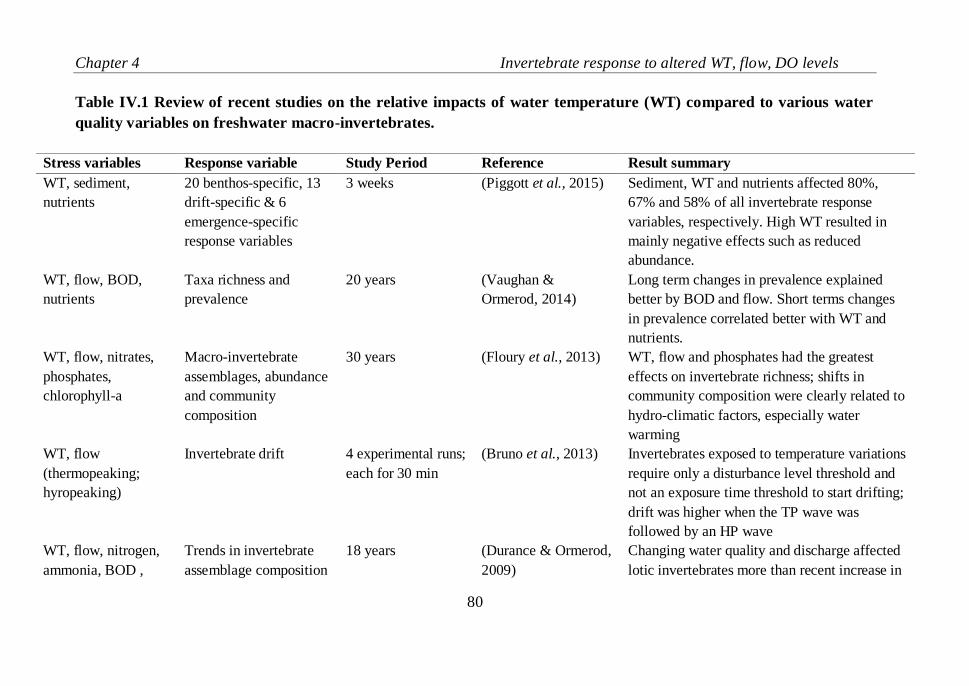
Chapter 4 Invertebrate response to altered WT, flow, DO levels
80
Table IV.1 Review of recent studies on the relative impacts of water temperature (WT) compared to various water
quality variables on freshwater macro-invertebrates.
Stress variables Response variable Study Period Reference Result summary
WT, sediment,
nutrients
20 benthos-specific, 13
drift-specific & 6
emergence-specific
response variables
3 weeks (Piggott et al., 2015) Sediment, WT and nutrients affected 80%,
67% and 58% of all invertebrate response
variables, respectively. High WT resulted in
mainly negative effects such as reduced
abundance.
WT, flow, BOD,
nutrients
Taxa richness and
prevalence
20 years (Vaughan &
Ormerod, 2014)
Long term changes in prevalence explained
better by BOD and flow. Short terms changes
in prevalence correlated better with WT and
nutrients.
WT, flow, nitrates,
phosphates,
chlorophyll-a
Macro-invertebrate
assemblages, abundance
and community
composition
30 years (Floury et al., 2013) WT, flow and phosphates had the greatest
effects on invertebrate richness; shifts in
community composition were clearly related to
hydro-climatic factors, especially water
warming
WT, flow
(thermopeaking;
hyropeaking)
Invertebrate drift 4 experimental runs;
each for 30 min
(Bruno et al., 2013) Invertebrates exposed to temperature variations
require only a disturbance level threshold and
not an exposure time threshold to start drifting;
drift was higher when the TP wave was
followed by an HP wave
WT, flow, nitrogen,
ammonia, BOD ,
Trends in invertebrate
assemblage composition
18 years (Durance & Ormerod,
2009)
Changing water quality and discharge affected
lotic invertebrates more than recent increase in
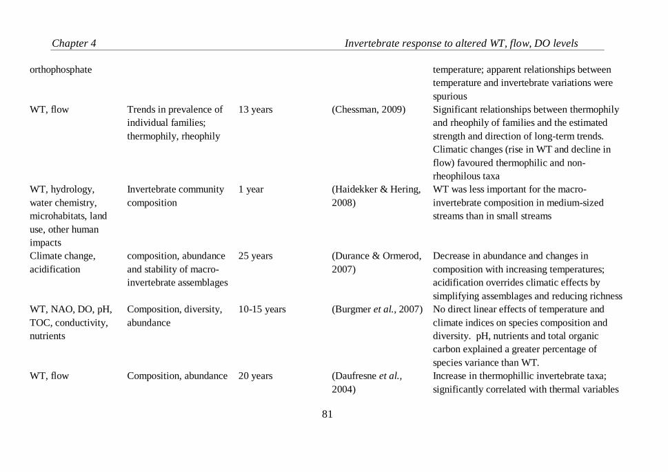
Chapter 4 Invertebrate response to altered WT, flow, DO levels
81
orthophosphate temperature; apparent relationships between
temperature and invertebrate variations were
spurious
WT, flow Trends in prevalence of
individual families;
thermophily, rheophily
13 years (Chessman, 2009) Significant relationships between thermophily
and rheophily of families and the estimated
strength and direction of long-term trends.
Climatic changes (rise in WT and decline in
flow) favoured thermophilic and non-
rheophilous taxa
WT, hydrology,
water chemistry,
microhabitats, land
use, other human
impacts
Invertebrate community
composition
1 year (Haidekker & Hering,
2008)
WT was less important for the macro-
invertebrate composition in medium-sized
streams than in small streams
Climate change,
acidification
composition, abundance
and stability of macro-
invertebrate assemblages
25 years (Durance & Ormerod,
2007)
Decrease in abundance and changes in
composition with increasing temperatures;
acidification overrides climatic effects by
simplifying assemblages and reducing richness
WT, NAO, DO, pH,
TOC, conductivity,
nutrients
Composition, diversity,
abundance
10-15 years (Burgmer et al., 2007) No direct linear effects of temperature and
climate indices on species composition and
diversity. pH, nutrients and total organic
carbon explained a greater percentage of
species variance than WT.
WT, flow Composition, abundance 20 years (Daufresne et al.,
2004)
Increase in thermophillic invertebrate taxa;
significantly correlated with thermal variables
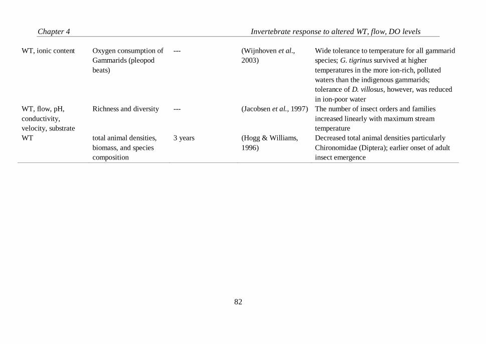
Chapter 4 Invertebrate response to altered WT, flow, DO levels
82
WT, ionic content Oxygen consumption of
Gammarids (pleopod
beats)
--- (Wijnhoven et al.,
2003)
Wide tolerance to temperature for all gammarid
species; G. tigrinus survived at higher
temperatures in the more ion-rich, polluted
waters than the indigenous gammarids;
tolerance of D. villosus, however, was reduced
in ion-poor water
WT, flow, pH,
conductivity,
velocity, substrate
Richness and diversity --- (Jacobsen et al., 1997) The number of insect orders and families
increased linearly with maximum stream
temperature
WT total animal densities,
biomass, and species
composition
3 years (Hogg & Williams,
1996)
Decreased total animal densities particularly
Chironomidae (Diptera); earlier onset of adult
insect emergence
Chapter 4 Invertebrate response to altered WT, flow, DO levels
83
4.3 Materials and methods
4.3.1 The set-up
The experiments were conducted in an experimental flume 3.0 m long, 0.80
m wide and 0.60 m deep made of 10 mm thick Perspex panels (Fig IV.1).
The flume was divided into three sub-channels, each serving as a replicate.
The observational area of each replicate was 0.65 m long, 0.25 m wide and
0.10 m deep. A water pump was attached to one end of the flume which
provided adjustable flows during the experiments. A mesh screen was
installed at the downstream and upstream ends of each observational area,
which prevented the escape of insects, and collected the drifting individuals.
Fine sand was glued on the bottom PVC plates to provide a suitable
colonization substrate for experimental animals.
Flow velocities were determined for each flow level at two locations (2 cm
above the bottom) in each compartment (upstream and downstream ends)
using an Acoustic Doppler Velocimeter (ADV; Micro ADV 16 MHz, 10 Hz
recording; Sontek, San Diego, CA, U.S.A.). Water temperature was regulated
by a thermostat heater attached to an immersion rod. Dissolved oxygen
concentrations were experimentally adjusted by bubbling air or nitrogen gas
through the water.
4.3.2 Invertebrate samples
Three species of invertebrates were selected for the experiments namely the
damselfly Banded Demoiselle Calopteryx splendens (Harris, 1782), the
‘demon shrimp’ Dikerogammarus haemobaphes (Eichwald, 1841) and the
caseless caddisfly Hydropsyche pellucidula (Curtis, 1834), based on their
abundance, body type and flow preferences. The invertebrates were collected
by hand nets from the River Spree. Individuals with similar body size were
selected for the experiments and kept in separate aquaria at 20°C.
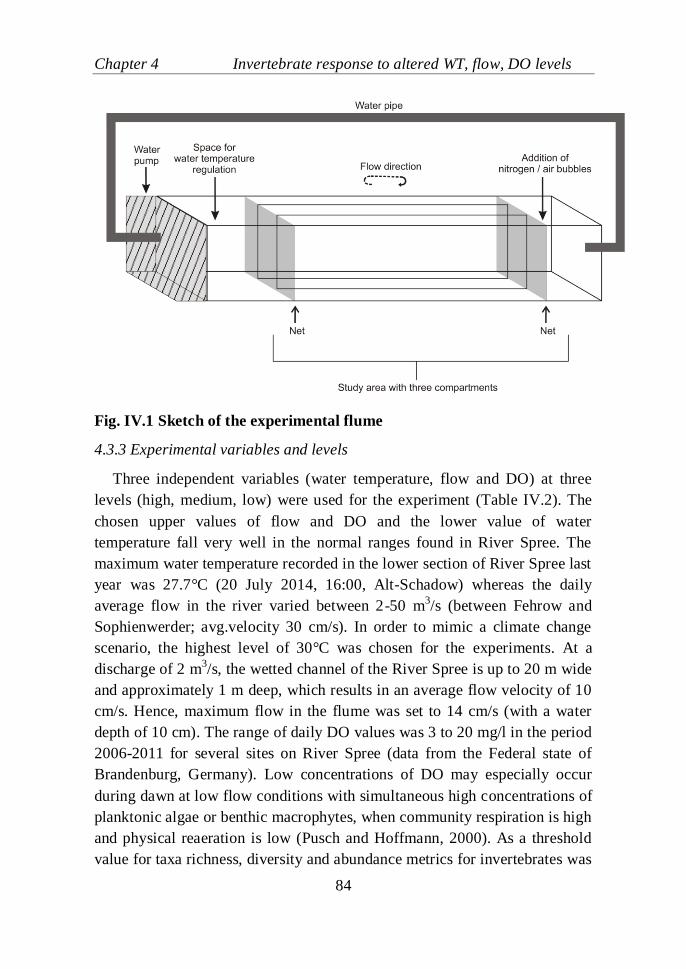
Chapter 4 Invertebrate response to altered WT, flow, DO levels
84
Fig. IV.1 Sketch of the experimental flume
4.3.3 Experimental variables and levels
Three independent variables (water temperature, flow and DO) at three
levels (high, medium, low) were used for the experiment (Table IV.2). The
chosen upper values of flow and DO and the lower value of water
temperature fall very well in the normal ranges found in River Spree. The
maximum water temperature recorded in the lower section of River Spree last
year was 27.7°C (20 July 2014, 16:00, Alt-Schadow) whereas the daily
average flow in the river varied between 2-50 m3/s (between Fehrow and
Sophienwerder; avg.velocity 30 cm/s). In order to mimic a climate change
scenario, the highest level of 30°C was chosen for the experiments. At a
discharge of 2 m3/s, the wetted channel of the River Spree is up to 20 m wide
and approximately 1 m deep, which results in an average flow velocity of 10
cm/s. Hence, maximum flow in the flume was set to 14 cm/s (with a water
depth of 10 cm). The range of daily DO values was 3 to 20 mg/l in the period
2006-2011 for several sites on River Spree (data from the Federal state of
Brandenburg, Germany). Low concentrations of DO may especially occur
during dawn at low flow conditions with simultaneous high concentrations of
planktonic algae or benthic macrophytes, when community respiration is high
and physical reaeration is low (Pusch and Hoffmann, 2000). As a threshold
value for taxa richness, diversity and abundance metrics for invertebrates was
Chapter 4 Invertebrate response to altered WT, flow, DO levels
85
found to be 2.6 mg/l for some lowland streams in North America (Justus et
al., 2014), a level of 2.7 mg/l was set as the lowest value for the experiments.
Table IV.2 Experimental levels of the aquatic variables subjected on
macro-invertebrate species to determine their responses.
Levels Temperature (°C) Flow (cm/s) Dissolved Oxygen (mg/L)
High 30 14 ± 1 >6.0
Medium 25 11 ± 1 4.0
Low 20 5 ± 0.5 2.7
4.3.4 Experimental runs
The total number of individuals used in the experiments for C. splendens, D.
haemobaphes and H. pellucidula, were 27 (9 in each replicate), 30 (10 in
each) and 30 (10 in each) respectively, which corresponded to average
densities of 49 ind. m-2
, 62 ind. m-2
and 62 ind. m-2
.
In total, we conducted three sub-sets of experiments. Within each subset, two
independent variables (two-way interaction) were altered at the three levels
for all possible combinations (9 combinations for each sub-set; total runs=
9*3=27). Number of drifting individuals was counted for each run as the
response/dependent variable. Each experimental run lasted for 40 minutes, or
until when 50% of the population had drifted. Drift observations were
recorded every 5 minutes. Between each run, a break of 15-20 min was kept
for the animals to de-stress and also to relocate the drifted individuals to their
initial locations. Suitable micro-habitats were provided for each species to
prevent detachments due to lack of surfaces to hold on to.
An additional sub-set of experiments was conducted for H. pellucidula (7
individuals in each replicate), in which ventilatory undulations where also
measured as response variable, along with drift. In these set of experiments,
two levels of temperature (T1= 25°C, T2= 30°C) and flow (F1= 10 cm/s, F2=
5 cm/s) were chosen and were varied at low DO (≤ 2mg/l). Each run lasted
for 30 min.
4.3.5 Data Analysis
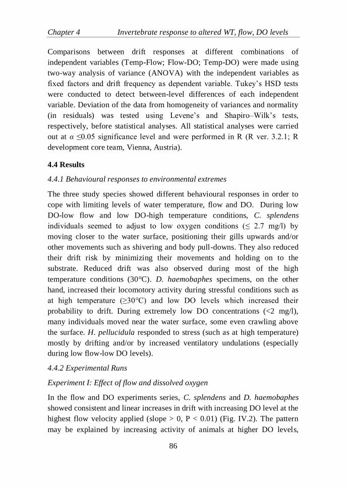
Chapter 4 Invertebrate response to altered WT, flow, DO levels
86
Comparisons between drift responses at different combinations of
independent variables (Temp-Flow; Flow-DO; Temp-DO) were made using
two-way analysis of variance (ANOVA) with the independent variables as
fixed factors and drift frequency as dependent variable. Tukey’s HSD tests
were conducted to detect between-level differences of each independent
variable. Deviation of the data from homogeneity of variances and normality
(in residuals) was tested using Levene’s and Shapiro–Wilk’s tests,
respectively, before statistical analyses. All statistical analyses were carried
out at α ≤0.05 significance level and were performed in R (R ver. 3.2.1; R
development core team, Vienna, Austria).
4.4 Results
4.4.1 Behavioural responses to environmental extremes
The three study species showed different behavioural responses in order to
cope with limiting levels of water temperature, flow and DO. During low
DO-low flow and low DO-high temperature conditions, C. splendens
individuals seemed to adjust to low oxygen conditions (≤ 2.7 mg/l) by
moving closer to the water surface, positioning their gills upwards and/or
other movements such as shivering and body pull-downs. They also reduced
their drift risk by minimizing their movements and holding on to the
substrate. Reduced drift was also observed during most of the high
temperature conditions (30°C). D. haemobaphes specimens, on the other
hand, increased their locomotory activity during stressful conditions such as
at high temperature (≥30°C) and low DO levels which increased their
probability to drift. During extremely low DO concentrations (<2 mg/l),
many individuals moved near the water surface, some even crawling above
the surface. H. pellucidula responded to stress (such as at high temperature)
mostly by drifting and/or by increased ventilatory undulations (especially
during low flow-low DO levels).
4.4.2 Experimental Runs
Experiment I: Effect of flow and dissolved oxygen
In the flow and DO experiments series, C. splendens and D. haemobaphes
showed consistent and linear increases in drift with increasing DO level at the
highest flow velocity applied (slope > 0, P < 0.01) (Fig. IV.2). The pattern
may be explained by increasing activity of animals at higher DO levels,
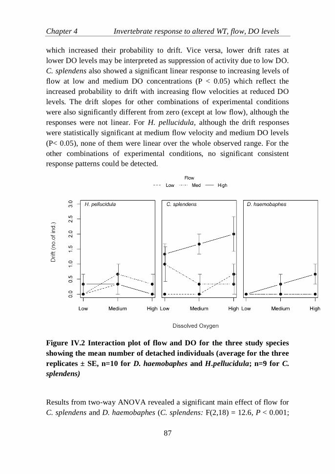
Chapter 4 Invertebrate response to altered WT, flow, DO levels
87
which increased their probability to drift. Vice versa, lower drift rates at
lower DO levels may be interpreted as suppression of activity due to low DO.
C. splendens also showed a significant linear response to increasing levels of
flow at low and medium DO concentrations (P < 0.05) which reflect the
increased probability to drift with increasing flow velocities at reduced DO
levels. The drift slopes for other combinations of experimental conditions
were also significantly different from zero (except at low flow), although the
responses were not linear. For H. pellucidula, although the drift responses
were statistically significant at medium flow velocity and medium DO levels
(P< 0.05), none of them were linear over the whole observed range. For the
other combinations of experimental conditions, no significant consistent
response patterns could be detected.
Figure IV.2 Interaction plot of flow and DO for the three study species
showing the mean number of detached individuals (average for the three
replicates ± SE, n=10 for D. haemobaphes and H.pellucidula; n=9 for C.
splendens)
Results from two-way ANOVA revealed a significant main effect of flow for
C. splendens and D. haemobaphes (C. splendens: F(2,18) = 12.6, P < 0.001;
Chapter 4 Invertebrate response to altered WT, flow, DO levels
88
D. haemobaphes: F(2,18) = 4.5, P = 0.03) whereas no significant main effect
of DO (C. splendens: F(2,18) = 0.6, P =0.5; D. haemobaphes: F(2,18) = 1.5,
P = 0.3) or interaction effect of flow and DO on the drift response (C.
splendens: F(4,18) = 1.2, P = 0.4; D. haemobaphes: F(4,18) = 1.5, P = 0.2)
could be detected. Between-level comparisons for flow showed that drift
responses at low flow and medium flow were significantly different from that
at high flow velocity for both C. splendens (P<0.01) and D. haemobaphes (P
= 0.04). None of the main effects of flow (F(2,18) = 0.6, P = 0.6) and DO
(F(2,18) = 1.8, P = 0.2) or the interaction effects (F(4,18) = 0.6, P = 0.7) were
significant for H. pellucidula.
Experiment II: Effect of water temperature and dissolved oxygen
In the case of varying water temperature and DO levels, C. splendens showed
a steady and significant increase in drift response with increasing DO levels
at low temperature (slope significantly different from zero, P < 0.01) (Fig.
IV.3). Drift responses to temperature were significant at all DO levels (P =
0.02), however a linear decrease with increasing temperature levels was seen
only at high DO level. C. splendens were seen to have minimized movements
and either positioned their setae upwards or shifted closer to the water surface
during the high temperature and low DO condition. D. haemobaphes showed
significant linear decrease with increasing DO levels at high temperature
(P<0.001), whereas a non-linear increase with increasing temperature levels
at low DO level (P = 0.02). Significant drift responses were observed for H.
pellucidula at all DO levels and temperature levels (except at low
temperature) (P< 0.05). However, the drift increased linearly with increasing
DO levels at high temperature and with increasing temperature levels at low
and high DO levels (Fig. IV.3).
Overall, water temperature had a significant (C. splendens: F(2,18) = 8.6, P =
0.002; D. haemobaphes: F(2,18) = 12, P < 0.001; H. pellucidula: F(2,18) =
9.1, P = 0.002 ), and DO had no significant main effect on drift responses for
all species (C. splendens: F(2,18) = 0.3, P = 0.8; D. haemobaphes: F(2,18) =
0.4, P = 0.7; H. pellucidula: F(2,18) = 1, P = 0.4). The interaction of
temperature and DO had a significant effect only on the drift response of D.
haemobaphes (F(4,18) = 3.4, P = 0.03), showing an amplified increase in
drift frequency at high temperature and under low DO concentrations,
whereas it was subdued under high DO levels.
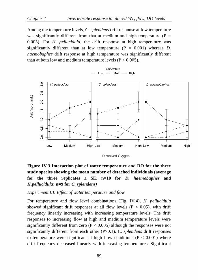
Chapter 4 Invertebrate response to altered WT, flow, DO levels
89
Among the temperature levels, C. splendens drift response at low temperature
was significantly different from that at medium and high temperature (P =
0.005). For H. pellucidula, the drift response at high temperature was
significantly different than at low temperature (P = 0.001) whereas D.
haemobaphes drift response at high temperature was significantly different
than at both low and medium temperature levels (P < 0.005).
Figure IV.3 Interaction plot of water temperature and DO for the three
study species showing the mean number of detached individuals (average
for the three replicates ± SE, n=10 for D. haemobaphes and
H.pellucidula; n=9 for C. splendens)
Experiment III: Effect of water temperature and flow
For temperature and flow level combinations (Fig. IV.4), H. pellucidula
showed significant drift responses at all flow levels (P < 0.05), with drift
frequency linearly increasing with increasing temperature levels. The drift
responses to increasing flow at high and medium temperature levels were
significantly different from zero (P < 0.005) although the responses were not
significantly different from each other (P>0.1). C. splendens drift responses
to temperature were significant at high flow conditions (P < 0.001) where
drift frequency decreased linearly with increasing temperatures. Significant
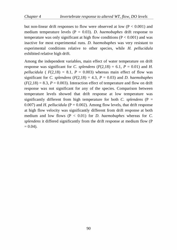
Chapter 4 Invertebrate response to altered WT, flow, DO levels
90
but non-linear drift responses to flow were observed at low (P < 0.001) and
medium temperature levels (P = 0.03). D. haemobaphes drift response to
temperature was only significant at high flow conditions (P < 0.001) and was
inactive for most experimental runs. D. haemobaphes was very resistant to
experimental conditions relative to other species, while H. pellucidula
exhibited relative high drift.
Among the independent variables, main effect of water temperature on drift
response was significant for C. splendens (F(2,18) = 6.1, P = 0.01) and H.
pellucidula ( F(2,18) = 8.1, P = 0.003) whereas main effect of flow was
significant for C. splendens (F(2,18) = 4.3, P = 0.03) and D. haemobaphes
(F(2,18) = 8.3, P = 0.003). Interaction effect of temperature and flow on drift
response was not significant for any of the species. Comparison between
temperature levels showed that drift response at low temperature was
significantly different from high temperature for both C. splendens (P =
0.007) and H. pellucidula (P = 0.002). Among flow levels, that drift response
at high flow velocity was significantly different from drift response at both
medium and low flows (P < 0.01) for D. haemobaphes whereas for C.
splendens it differed significantly from the drift response at medium flow (P
= 0.04).
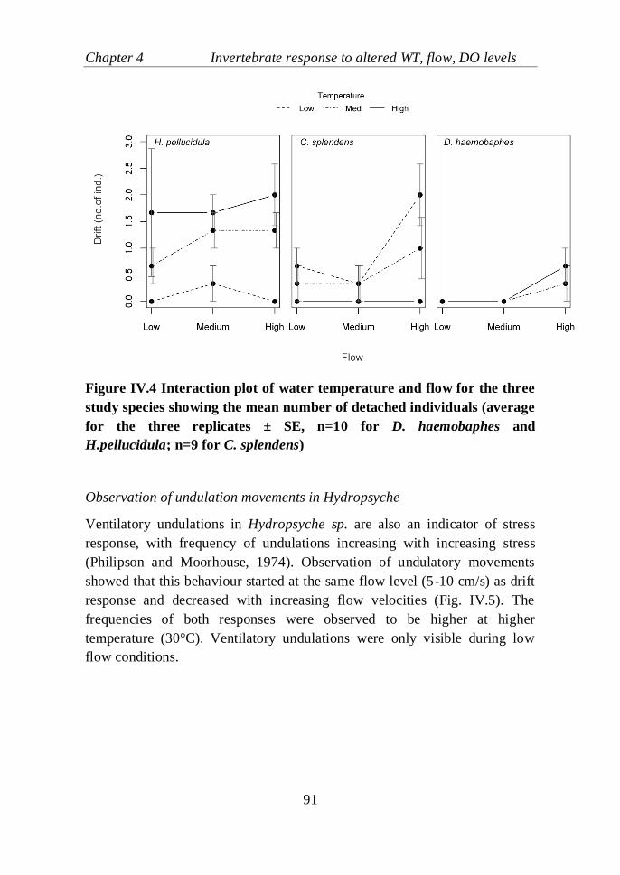
Chapter 4 Invertebrate response to altered WT, flow, DO levels
91
Figure IV.4 Interaction plot of water temperature and flow for the three
study species showing the mean number of detached individuals (average
for the three replicates ± SE, n=10 for D. haemobaphes and
H.pellucidula; n=9 for C. splendens)
Observation of undulation movements in Hydropsyche
Ventilatory undulations in Hydropsyche sp. are also an indicator of stress
response, with frequency of undulations increasing with increasing stress
(Philipson and Moorhouse, 1974). Observation of undulatory movements
showed that this behaviour started at the same flow level (5-10 cm/s) as drift
response and decreased with increasing flow velocities (Fig. IV.5). The
frequencies of both responses were observed to be higher at higher
temperature (30°C). Ventilatory undulations were only visible during low
flow conditions.
Chapter 4 Invertebrate response to altered WT, flow, DO levels
92
Figure IV.5 Interaction plot of temperature and flow at low DO level (< 2
mg/l) for H. pellucidula showing the number of individuals detached and
the number of individuals showing respiratory undulations (average for
the three replicates ± SE, n=7).
4.5 Discussion
4.5.1 Behavioural responses to multiple environmental stressors
For most organisms, one of the first and most sensitive responses to stress is
through changes in behaviour which is a biochemical reaction controlled by
neurological and hormonal pathways (Gerhardt 1996; Boyd et al., 2002).
Behavioural responses are linked to ecological consequences in a system at
every level (Gordon, 2010), be it at the organism (e.g. reduced performance),
population (e.g. reproduction success, emergence) or community levels (e.g.
predation) (Gerhardt, 1996). Changes in behaviour due to aquatic
stress/pollution include increased downstream invertebrate drift, avoidance,
changes in gill ventilation, feeding rates and locomotion (Brittain and
Eikeland 1988; Gerhardt 1996; Boyd et al., 2002).
In this experiment, the drift frequency of three invertebrate species was
measured as a stress response to varying levels of water temperature, flow
and DO. Drift is an important mechanism for benthic invertebrate dispersal
and colonization and also as an avoidance and escape strategy from life
threatening conditions (Townsend and Hildrew, 1976). It affects various
Chapter 4 Invertebrate response to altered WT, flow, DO levels
93
aspects of their population dynamics and serves as an important pathway for
energy transfer within river systems (Gibbins et al., 2010). During the
experiment, we noted that the study species responded differently to stress
and not necessarily by drifting. The caseless caddisfly H. pellucidula
responded to stressful conditions mostly by drifting or by increasing
ventilatory undulations. Highest drift frequencies were observed at high
water temperature (30°C) regardless of flow and DO levels, whereas the
characteristic ventilatory undulations (Phillipson and Moorhouse 1974) were
triggered during low flow (≤ 5cm/s) and low DO (< 2.7 mg/l) conditions.
These undulations increased with water temperature, a result also observed
by Phillipson and Moorhouse (1974). Hydropsyche sp. is among the
dominant drifting invertebrates (Wetzel, 2001) and has been shown to
tolerate temperatures up to 28°C (Sherberger et al., 1977) and low oxygen
concentrations below 2 mg/l (Connolly, Crossland and Pearson, 2004,
Philipson and Moorhouse, 1974). Since it is a rheophilic species, it can
sustain high velocities up to at least 60 cm/s and low flow velocities down to
5±2 cm/s (Philipson and Moorhouse, 1974; Brunke et al., 2001). This could
explain why more significant responses where observed for temperature than
for other variables.
The damselfly C. splendens, on the other hand, showed little activity during
stressful conditions. During high temperature (30°C) and reduced flow (5
cm/s) or DO (≤ 2.7 mg/l) levels, C. splendens showed little or no drifting due
to minimization of movement. An explanation could be that animals tend to
reduce their activity and wait at reduced metabolic rates for conditions to
improve (Connolly et al., 2004). Other behavioural responses such as vertical
migration, shivering, especially during low DO levels, were also observed.
Such behaviour provide additional flexibility for the animals to deal with
hypoxia (Apodaca and Chapman, 2004). On the contrary, increased
movement (locomotion, fighting), and hence drift, was observed during
suitable conditions such as during low temperature and high flow/DO levels.
Drifting due to loss of foothold during such activities could explain
increasing drift rates in favourable conditions (behavioural drift). In general,
Calopteryx sp. is known to tolerate velocities up to 77 cm/s (Dorier and
Vaillant (1953/1954), Schnauder et al., 2010). It is also tolerant to high water
temperatures up to 30°C under normal oxygen conditions (Verberk and
Chapter 4 Invertebrate response to altered WT, flow, DO levels
94
Calosi, 2012) and can survive low DO levels through behavioural responses
(Apodaca and Chapman, 2004; Miller, 1993).
The amphipod crustacean D. haemobaphes, in general, showed lack of any
activity and spent most time sheltered in the crevices of the flume. During
stressful conditions (high temperature and low DO), the individuals showed
increased locomotion. It appears that Dikerogammarus sp. is relatively
inactive species (Gabel et al., 2011; Maazouzi et al., 2011) spending most
their time sheltered under stones or other similar substrates. It has been
shown to tolerate temperatures up to 27-30°C (Kititsyna, 1980; Wijnhoven et
al., 2003; Maazouzi et al., 2011). It requires highly oxygenated waters (Boets
et al., 2010) and is comfortable in the velocity range of 8-16 cm/s (Schnauder
et al., 2010).
4.5.2 Temperature stress in a multiple stressor context
Alteration of water temperature with flow or DO resulted in significant
effects on the study species. During temperature and flow alterations, both
temperature and flow had a main significant effect on two out of three
species. Lack of any interaction between water temperature and flow
indicates that negative impacts of high water temperatures were not offset by
increasing flows and vice versa. Water temperature, when varied along with
DO, had a significant main effect on all three species whereas DO had no
significant effect. Interaction among variables was detected for temperature
and DO only in the case of D. haemobaphes indicating that negative impacts
of high water temperatures were amplified under low DO conditions whereas
were offset at high DO levels. Aquatic ectotherms which lack efficient
respiration techniques (such as Dikerogammarus sp. which require high
oxygen levels) are especially vulnerable to the multiple stressor effects of
increased water temperatures and reduced levels of oxygen (Verberk and
Bilton, 2013). These results demonstrate that water temperature, in the given
set of experimental conditions, had a greater effect than any of the other
variables in a multiple stressor context. Among coupled variable effects, our
results indicate that on a short time scale, concomitant variation of water
temperature and flow will have stronger impacts than when temperature and
DO or flow and DO are varied together.
Several other experimental studies on water temperature effects corroborate
these conclusions. Phillipson & Moorhouse (1974) observed ventilatory and
Chapter 4 Invertebrate response to altered WT, flow, DO levels
95
net-spinning activities of three Hydropsychidae species under varying water
temperature (2-25°C), flow (0-40 cm/s) and DO (1-10 mg/l) levels. From
their study, they concluded that although flow will be important in
determining the micro-distribution of the species, water temperature is likely
to play a more important role in successional and geographical distribution,
with DO operating in particular circumstances. Hogg and Williams (1996)
conducted a large scale field experiment in which they investigated the
effects of thermal manipulation on the total invertebrate densities, biomass,
and species composition. They found that small changes in water temperature
resulted in measurable responses by the resident invertebrate populations
such as reductions in total densities, increased growth rates, earlier
emergence, precocious breeding, decreases in body size at maturity, and
altered sex ratios. They also observed variable responses of individual species
to the manipulation suggesting that responses to changes in temperature are
not universal and may be more prevalent within certain groups. Within
geothermal streams as well, water temperature of geothermal fluids had a
greater influence than the chemical component in determining benthic
community features in Big Sulphur Creek, significantly altering benthic
community structure and macroinvertebrate density (Lamberti and Resh,
1983). In a more recent study by Piggot et al. (2015), experimental
simulations showed that among sediment, water temperature and nutrients,
water temperature was the second-most impacting variable on
macroinvertebrate community dynamics. It affected 67% of the 39 measured
response variables including drift EPT richness. Increasing water temperature
negatively affected drift EPT richness, drift body size, total abundance, total
EPT abundance whereas positively affected community diversity and
evenness. Interactive effects of water temperature with nutrients and/or
sediments were also significant for several response variables such as total
drift propensity and emergence.
Results from some observational studies also support these results.
Investigation of water quality factors affecting invertebrate community
structure and composition over 30 years revealed that water warming
explained a greater percentage of variance irrespective of taxonomic-based
metric than discharge (Floury et al., 2013). Durance and Ormerod (2007) also
observed significant declines in abundance and changes assemblage
composition with increasing temperatures over a 25-year period. Vaughan
Chapter 4 Invertebrate response to altered WT, flow, DO levels
96
and Ormerod (2014) found that short-term variations in taxon prevalence
correlated primarily with temperature and nutrient concentrations while long-
term (21 years) increases or decreases in taxon prevalence correlated better
with discharge and pollution sensitivity. Similar results have been also
observed for other aquatic biota as well. For example, Wenger et al. (2011b)
showed that temperature increases themselves played a dominant role over
flow in driving future declines of cutthroat trout, brook trout, and rainbow
trout fish species. However, some other studies (Burgmer et al., 2007;
Durance and Ormerod, 2009; Dohet et al., 2015) reported that water quality,
discharge and land-use had larger effects on invertebrate assemblage
composition than temperature highlighting that long-term temperature effects
become apparent in better water quality conditions. These results also suggest
that the time scale over which the multiple stressor effects are studied might
influence the group of factors responsible for the ecological responses
observed. The lack of interaction effects observed between temperature-flow
and flow-DO in our experiment might also be a result of the choice of time
scale.
The results of this experiment are particularly relevant when viewed in
relation with hydro-climatic extreme events, which occur at short time scales.
Our results suggest that when heat wave (high water temperature) is
accompanied with drought-like conditions (low flow) for short periods of
time, the effect of heat wave might override the low flow effects for certain
species (H. pellucidula) while low flow effects might dominate or act along
with heat wave effects for some other species (C. splendens, D.
haemobaphes). Such impacts of coinciding extreme events might lead to
abrupt changes in species compositions and distributions and might affect
future responses of the ecosystem to similar events (Leigh et al., 2014).
4.6 Conclusion
Although already several studies have addressed the issue of multiple
stressors on river ecosystems, studies specifically looking into multiple
effects of water temperature along with other stressors are relatively scarce.
Despite the short time scale of the study, several significant results were
detected. In general, our experiment showed dominant effects of water
temperature over flow and DO and dominant water temperature-flow effects
on the behavioural responses of three lowland invertebrate species on short
Chapter 4 Invertebrate response to altered WT, flow, DO levels
97
time scales. However, the main and interactive impacts of multiple stressors
varied across species depending on their tolerance ranges for water
temperature, flow and DO and induced different behavioural responses. We
conclude that the effects of human-induced shifts in river water temperature
on benthic invertebrates may be modified by concomitant limiting conditions
of DO and flow, but that those interactions highly depend on the
physiological and behavioural patterns of species, and on the stress level
range involved. Available information suggests that interactions of multiple
stressors may occur at larger spatial and temporal scales, too, but which
needed a much larger design to be demonstrated experimentally.
Acknowledgements
Roshni Arora was funded by the SMART Joint Doctoral Programme which is
financed by the Erasmus Mundus programme of the European Union. This
work is also part of the MARS project (Managing Aquatic ecosystems and
water Resources under multiple Stress) funded under the 7th EU Framework
Programme, Theme 6 (Environment including Climate Change), Contract
No.: 603378 (http://www.mars-project.eu). We thank Marlen Mährlein,
Jürgen Schreiber for the flume set up, sample collection; Francesca Pilotto is
thanked for her help during sorting and advice on experimental runs.
Chapter 5 General discussion
98
5. GENERAL DISCUSSION
5.1 Rationale and research aims
River systems worldwide are threatened as a result of climate change and
anthropogenic modifications which impact thermal and hydrological regimes
(Ormerod et al., 2010). A significant rise in water temperature has been
reported for several rivers in the past decades (Webb and Nobilis, 2007;
Kaushal et al., 2010; Isaak et al., 2012, Orr et al., 2014) and this trend is
expected to continue in the future (van Vliet et al., 2013). Given the crucial
role that river temperature plays in governing several river processes,
understanding the dynamics, processes, controls and drivers of change of
river thermal regimes is of prime importance. Several previous studies on
river temperature have helped gain insight on the primary controls of river
temperature behaviour and the direct/indirect impacts of environmental
changes on river temperature. However, there is still a need to further
improve our understanding of the spatial and temporal heterogeneity in river
temperatures (Webb et al., 2008). More precisely, the role of hydro-
climatological (such as air temperature, flow) and landscape variables (such
as land use, altitude) in causing river temperature heterogeneity over a range
of temporal and spatial scales needs to be further clarified. Furthermore, river
systems are exposed to an array of stressors, which interact in complex ways
to result in either synergistic, antagonistic or no net effects on freshwater
biodiversity (Ormerod et al., 2010; Jackson et al., 2015). While a few studies
have investigated the long-term impacts of multiple stressors on freshwater
biota, studies investigating the short-term impacts of simultaneously
changing physical aquatic parameters such as water temperature, flow and
dissolved oxygen, on freshwater macroinvertebrates are extremely scarce.
Therefore, this thesis aimed to address these gaps by observing and
quantifying river temperature changes over several spatial and temporal
scales. In Chapter 2, long-term (25 years) and short-term changes (10 years)
in river water temperature were quantified and the roles of climatic,
hydrological and landscape variables were identified for German rivers on a
regional basis. In Chapter 3, spatial heterogeneity in water temperature of a
lowland river reach (~200 km) was observed and quantified via a heat-budget
Chapter 5 General discussion
99
model and a semi-empirical model over a period of nine months. In addition,
the role of landscape factors in causing the observed heterogeneity was
investigated. Furthermore, the efficacy of riparian shading in moderating
river temperature downstream of lakes was tested. In Chapter 4, the
behavioural response (namely drift) of three river macroinvertebrate species
to varying levels of water temperature, flow, and dissolved oxygen, and to
combinations of these factors were experimentally investigated to
characterize the relative influence of rising water temperature in a multiple-
stressor context.
5.2 Key research findings
The novelty of the research presented in this thesis lies in: (a) conducting the
first assessment of long-term and short-term changes in river temperature for
Germany and identifying the contribution of air temperature changes, flow
changes, changes in climatic phenomena (such as the North Atlantic
Oscillation) and landscape variables (such as altitude, catchment area,
ecoregion, land use), in the observed changes in river temperature; (b)
assessing the influence of the presence and lateral extent of different types of
land use (such as forested, agricultural and urban areas) and other landscape
features (such as lakes) in inducing reach-scale thermal heterogeneity and
quantifying the observed heterogeneity using a simple heat budget and a
semi-empirical model; (c) presenting the first assessment of short-term
impacts of simultaneous changes in water temperature, flow and dissolved
oxygen on behavioural responses of three lowland benthic invertebrate
species. The key research outcomes are as follows:
a) Chapter 2: The majority of the analysed sites have undergone
significant warming in the past 25 years in Germany, with the
following significant controls identified at the regional scale:
i. Air temperature increase is the major driver of increasing river
temperature and of river temperature variability at most of the
studied sites, with its influence increasing with increasing
catchment area and at lower altitudes.
ii. Flow was identified as the second most important control of
river temperature variability, and its contribution in river
warming was more important for areas with low water
availability (specific runoff).
Chapter 5 General discussion
100
iii. Landscape variables such as altitude, catchment area and
ecoregion induced spatial variability in the magnitude of river
temperature changes via affecting the sensitivity of river
temperature to its local climate.
iv. The length of the study period has a significant impact on the
direction and rate of temperature change. Trends identified for
short time series of different lengths or different start and end
years are difficult to compare.
b) Chapter 3: The presence of urban areas and lakes were the most
important variables causing spatial river temperature heterogeneity
within the ~200 km reach of a lowland river. On the contrary,
whereas riparian buffer only had very limited effect on the river
temperature.
i. Urban areas and lakes acted as a heat source, in particular,
during the summer months. The impact of urban area on river
temperature did not depend on the lateral spatial extent along
the river, at least when present within 1 km from the river
edge.
ii. Riparian shading, even when present at up to 20 km
longitudinally, reduced maximum river temperatures only by
1°C below lakes, mainly because of the influence of advected
heat from the upstream lake which lasts over long distances.
This questions the efficacy of riparian shading in moderating
river temperatures in such reaches.
iii. In general, upstream conditions determined the base (or
average) river temperature at a site, while climatological
variations caused deviations around the base temperature.
c) Chapter 4: The three macroinvertebrate species showed different
behavioural responses to stressful conditions (such as high
temperature, low flow, low dissolved oxygen levels) and not
necessarily with drift. Main effects of water temperature and flow
were significant for two out of three species for paired stressor
combinations whereas the applied low dissolved oxygen levels only
produced a significant response when combined with other stressors.
Interaction between variables was detected only for temperature and
dissolved oxygen for a single species (Dikerogammarus
Chapter 5 General discussion
101
haemobaphes), with low dissolved oxygen amplifying the negative
impacts of high water temperature.
5.3 Synthesis
5.3.1 Temporal and spatial heterogeneity in river temperature behaviour
Temperature at a particular point in space and time in a channel is a function
of heat load and river flow or volume (Poole and Berman, 2001). Variations
in heat exchange processes and the volume of water in a channel can
determine short-term and long-term trajectories of river water temperature.
The results of this study revealed considerable spatial heterogeneity in
temporal river temperature behaviour at both regional and reach scales within
Germany. At the regional scale, a majority of the analysed sites on northern
German rivers showed a long-term increase in river temperature over time,
while a minority showed a decrease (Chapter 2). A similar pattern was
observed at seasonal and decadal time scales, as river temperature increased
for most of the sites across all seasons and decades. The observed temporal
changes in river temperature were attributed to temporal changes in air
temperature in general, as air temperature also exhibited increasing trends
and was the major control of seasonal and annual variability in river
temperature. Air temperature change has been observed to the major driver of
river temperature change for several other rivers in North America and
Europe as well (Webb and Nobilis, 2007; Kaushal et al., 2010; Orr et al.,
2014; Rice and Jastram, 2015). The other climatic variable, North Atlantic
Oscillation (NAO), which dictates much of the winter variability in air
temperature in the Northern Hemisphere (Hurrell, 2003), had a considerable
indirect influence on the inter-annual winter variability in river temperature
and possibly influenced changes in water temperature during the first decade
(1985-1995). River flow was found to have a significant influence on
seasonal variability of river temperature over both long and short time
periods. Flow is generally seen to have an inverse relationship with water
temperature (Chapter 2 and 3; Webb et al., 2003; van Vliet et al., 2011), with
greater flows leading to cooler water temperatures. However, the role of
increasing flows in moderating the rate of river temperature change over a
long time period and at a large spatial scale was indiscernible (Chapter 2), as
the greatest impact of flow is seen at shorter time scales (Webb et al., 2003)
and declines for very large catchments (Gu et al., 1998). Flow reductions (i.e.
Chapter 5 General discussion
102
reduction in thermal or assimilative capacity of rivers) were suggested to
have a clearer influence on long-term river warming at smaller spatial scales
(e.g., NE German rivers, Chapter 2; van Vliet et al., 2011). Spatial
heterogeneity in the magnitude of long term river temperature change was
mostly controlled by spatial differences in altitude, ecoregion and catchment
area. Higher river thermal sensitivity (thereby greater river warming) was
observed within larger catchment areas and at lower altitudes (lowland
rivers), as thermal sensitivity is a function of river size, velocity and water
volume (Webb et al., 2008; Kelleher et al., 2012). Higher residence times
(quicker rate of reaching equilibrium with air temperatures) and the effect of
upstream advected heat (accumulation of the heat in the entire stream
network; Chapter 3) contribute to high thermal sensitivity of lowland rivers.
At the reach scale, i.e., within a 200 km reach of a lowland river, the
investigated sites showed similar temporal behaviour over a period of nine
months (Chapter 3). Among the hydro-climatological variables, air
temperature was the major control of river temperature, similar to what
observed at the regional scale (Chapter 2). Weaker air-water temperature
correlations were observed in the downstream direction, primarily as the heat
advected from the upstream reaches becomes more dominant part of the heat
content in the channel. Spatial heterogeneity was observed in the magnitude
of daily and monthly means of river temperature along the reach, which was
mainly attributed to landscape variables. Spatial location of urban areas and
lakes defined the spatial heterogeneity within the reach (rather than presence
of riparian buffer), as sub-reaches flowing through these structures were
warmer in general and also attained the highest maximum temperatures as
compared to the sub-reaches without them. Urban areas act as a heat source
as the air and ground temperature tend to be higher than in rural areas and
also due to warm water additions from industries and runoff from hot
pavements (Pickett et al., 2001; Somers et al., 2013). Shallow lakes, such as
those found in the study reach, present a greater surface area to volume ratio
and a longer residence time (compared to rivers) for receiving atmospheric
heat inputs, thereby reaching equilibrium with atmospheric conditions at a
faster rate. Additionally, water temperatures at lake outlets are more
influenced by water temperature of the much shallower lakeshore. Although
the proportion of riparian buffer was negatively correlated with river
temperature, the effective buffer width was unclear. Also, riparian buffer did
Chapter 5 General discussion
103
not appear to effectively reduce the maximum and mean temperature below
lake affected sub-reaches, mainly as the influence of heat advected from
lakes lasts over large distances (at least ~20 km).
5.3.2 River temperature in a multiple stressor context
As especially observed for the lowland rivers in Germany, rising river
temperatures are majorly a result of high sensitivity to warmer air
temperatures, supplemented by reducing flows, particularly summer flows
(Chapter 2; van Vliet et al., 2011). Water temperatures can reach critically
high values for freshwater biodiversity during such conditions. In presence of
multiple stressors such as reduced flows and dissolved oxygen levels, water
temperature has the greatest influence as compared to the other two variables
on the behavioural response of freshwater macroinvertebrates (Hydropsyche
pellucidula, Calopteryx splendens, Dikerogammarus haemobaphes) on short
time scales (Chapter 4). This result particularly highlights the importance of
heat-related extreme events, where high temperatures are experienced for
short time periods. The behavioural responses of the three macoinvertebrates
to stress differed among species, with H. pellucidula responding by drifting,
C. splendens responding by inactivity and D. haemobaphes responding by
increased locomotion. Among coupled variable effects, the results indicated
that concomitant variation of water temperature and flow will have stronger
impacts than when temperature and DO or flow and DO vary together. The
interactive effects of these variables are, however, highly dependent on the
physiological and behavioural traits of a species, and on the stress level
involved (Chapter 4).
5.4 Implications for river ecosystem management
Results from the research presented in this thesis add to the growing
consensus that river warming is a global phenomenon. Climate change is not
suggested to be the sole reason for the observed warming and is rather a
result of complex interactions between climate patterns, anthropogenic
activities and sensitivity of a river to its environment (Chapter 2; Hannah et
al., 2015). Thermal and hydrological regime changes due to changing climate
and human activities are one of the major factors threatening the functioning
of freshwater ecosystems and the services they provide (Fig. V.1). More
specifically, the greatest impacts can be expected during low flows and
increased water temperature conditions (Chapter 4; van Vliet et al., 2011),
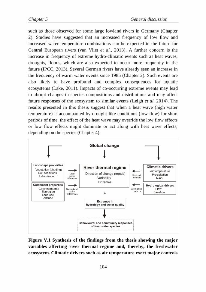
Chapter 5 General discussion
104
such as those observed for some large lowland rivers in Germany (Chapter
2). Studies have suggested that an increased frequency of low flow and
increased water temperature combinations can be expected in the future for
Central European rivers (van Vliet et al., 2013). A further concern is the
increase in frequency of extreme hydro-climatic events such as heat waves,
droughts, floods, which are also expected to occur more frequently in the
future (IPCC, 2013). Several German rivers have already seen an increase in
the frequency of warm water events since 1985 (Chapter 2). Such events are
also likely to have profound and complex consequences for aquatic
ecosystems (Lake, 2011). Impacts of co-occurring extreme events may lead
to abrupt changes in species compositions and distributions and may affect
future responses of the ecosystem to similar events (Leigh et al. 2014). The
results presented in this thesis suggest that when a heat wave (high water
temperature) is accompanied by drought-like conditions (low flow) for short
periods of time, the effect of the heat wave may override the low flow effects
or low flow effects might dominate or act along with heat wave effects,
depending on the species (Chapter 4).
Figure V.1 Synthesis of the findings from the thesis showing the major
variables affecting river thermal regime and, thereby, the freshwater
ecosystem. Climatic drivers such as air temperature exert major controls
Chapter 5 General discussion
105
on river temperature and act at regional scales while hydrological
controls, such as flow, act sub-regionally, having a substantial influence
on river temperature variability. Landscape and catchment properties
induce local and sub-regional spatial differences in climate, hydrology
and river morphology and thereby, river thermal regimes. Global
changes caused by human activities can affect river thermal regimes
directly as well indirectly via affecting any one or more of the mentioned
controls. Extremes in river temperatures and other important water
quality parameters, such as flow and dissolved oxygen, due to such
environmental changes can induce several behavioural responses in
freshwater species, ultimately affecting the entire ecosystem as a whole.
A major proportion of (60% of 1648 species) European freshwater species is
expected to lose at least 50% of their suitable habitat by 2050 due to climate
change impacts, including river warming (Markovic et al., 2014). The results
from this research suggest that river temperature behaviour of lowland rivers
is the most susceptible to changing climate (Chapter 2). Lowland rivers, such
as River Spree, are further subjected to additional pressures such as local
impacts of urbanization, discharge of warm water from shallow lakes and the
cumulative effect of advected heat (Chapter 3). Therefore, urgent measures
are needed to prevent or reduce the effect of environmental change on river
temperatures. Several measures have been suggested in the literature to
reduce river water temperatures. They include riparian buffer plantation
(Hrachowitz et al., 2010; Broadmeadow et al., 2011; Imholt et al., 2013;
Garner, 2014), restoration of floodplain connectivity and natural channel
geomorphology (Poole and Berman, 2001), cold water releases from
reservoirs (Isaak et al., 2012), and increase in discharge/decrease in
abstraction (Gu et al., 1998; Poole and Berman, 2001). Riparian buffer
plantation is widely recognized as a possible climate adaptation option by the
forestry sector in North America and, more recently, in the UK as well
(Johnson and Wilby, 2015). For headwater rivers, riparian buffers have been
suggested to be most effective in moderating maximum water temperatures
(Hrachowitz et al., 2010; Garner, 2014). For mid-sized to large lowland
rivers, the efficacy of riparian buffer is reduced or negligible as the canopy
cover is unable to effectively shade these rivers due to increased river width.
Plantation of riparian buffers along headwater rivers has also been suggested
Chapter 5 General discussion
106
to contribute to lower water temperature in the lowland rivers and also
throughout river basins (Hrachowitz et al., 2010; Garner, 2014). However,
this would probably be less effective for lowland rivers where buffer areas
are dominated by urban cover and those flowing through shallow lakes, as
these structures have been observed to cause warmer river temperatures
(Chapter 3; Mellina et al., 2002; Somers et al., 2013; Booth et al., 2014).
Also, riparian buffers were observed not to be very effective in reducing
water temperatures below lakes as the heat advected from the lakes plays a
more dominating influence (Chapter 3).
Therefore, for lowland rivers in general, river temperature could be managed
through flow manipulation (prevention of low flows), sustainable waste water
inputs, through the restoration and plantation of riparian buffers (for small
lowland rivers) and through the protection and conservation of high altitude
rivers (e.g. via flow protection and riparian buffer plantation), as river
temperature response in lowland catchments is a combination of local as well
as upstream conditions. For lowland reaches influenced by shallow lentic
structures and urban areas, additional or alternative measures such as
improving the groundwater recharge, managing the temperature of urban
discharges or creating shaded artificial ponds may be more effective and are
thus suggested.
References
107
References
ADV, 2012. Arbeitsgemeinschaft der Vermessungs-verwaltungen der Länder der
Bundesrepublik Deutschland: Erläuterungen zum ATKIS-Objektartenkatalog der
Arbeitsgemeinschaft der Vermessungsverwaltungen der Länder der Bundesrepublik
Deutschland. Available at: http://www.adv-online.de/Geotopography/ATKIS/
Alvarez D, Nicieza AG.2005. Compensatory response ‘defends’ energy levels but not
growth trajectories in brown trout, Salmo trutta L. Proceedings of the Royal Society B:
Biological Sciences 272: 601–607
Apodaca CK, Chapman LJ. 2004. Larval damselflies in extreme environments:
Behavioral and physiological response to hypoxic stress. Journal of Insect Physiology
50 (9): 767–775
Arismendi I, Johnson SL, Dunham JB, Haggerty R, Hockman-Wert D. 2012. The
paradox of cooling streams in a warming world: Regional climate trends do not parallel
variable local trends in stream temperature in the Pacific continental United States.
Geophysical Research Letters 39, L10401.
Arismendi I, Safeeq M, Dunham JB, Johnson SL. 2014. Can air temperature be used to
project in fl uences of climate change on stream temperature ? Environmental Research
Letters 9(8): 084015
Arnell NW, Gosling, SN. 2013. The impacts of climate change on river flow regimes at
the global scale. Journal of Hydrology 486:351-364.
Arscott DB, Tockner K, Ward J V. 2001. Thermal heterogeneity along a braided
floodplain river (Tagliamento River, northeastern Italy). Canadian Journal of Fisheries
and Aquatic Sciences 58 (12): 2359–2373.
Ashizawa D, Cole JJ. 1994. Long-term temperature trends for the Hudson River: a study
of the historical data. Estuaries 17(1): 166–71.
Bärlocher F, Seena S, Wilson KP, Williams DD. 2008. Raised water temperature lowers
diversity of hyporheic aquatic hyphomycetes. Freshwater Biology 53:368–379.
Benson NG. 1953. The importance of ground water to trout populations in the Pigeon
River, Michigan. (Ed J.B. Trefethen) In: Transactions of the Eighteenth North American
Wildlife Conference, pp. 269–281, Washington, DC, March 9, 10, and 11, 1953. Wildlife
Management Institute, Wire Building, Washington 5, DC.
Benyahya L, Caissie D, St-hilaire A, Ouarda TBMJ, Bobée B. 2007. A Review of
Statistical Water Temperature Models. Canadian Water Resources Journal 32(3): 179–
192
References
108
Boets P, Lock K, Messiaen M, Goethals PL. 2010. Combining data-driven methods and
lab studies to analyse the ecology of Dikerogammarus villosus. Ecological Informatics
5(2), 133-139.
Booth DB, Kraseski KA, Rhett JC. 2014. Local-scale and watershed-scale determinants
of summertime urban stream temperatures. Hydrological Processes 28(4): 2427–2438.
Bormann H. 2010. Runoff regime changes in German rivers due to climate change.
Erdkunde 64(3):257-279.
Boyd WA, Brewer SK, Williams PL. 2002. Chapter 8: Altered Behaviour of
Invertebrates Living in Polluted Environments. In: Behavioural ecotoxicology by
Dell'Omo, G. John Wiley & Sons.
Brezonik PL. 1972. Chemical kinetics and dynamics in natural water systems. In
:Ciaccio, L.L. (Ed.), Water and Wafer Pollution Handbook. Vol. 3. Marcel Dekker, New
York. pp. 831-913.
Brittain JE, Eikeland TJ. 1988. Invertebrate drift - A review. Hydrobiologia 166:77–93.
Broadmeadow SB, Jones JG, Langford TEL, Shaw PJ, Nisbet TR. 2011. The influence
of riparian shade on lowland stream water temperatures in southern England and their
viability for brown trout. River Research and Applications 27: 226–237.
Brown GW, Krygier JT. 1970. Effects of clear-cutting on stream temperature. Water
Resources Research 6:1133–1139.
Brown GW. 1969. Predicting temperatures of small streams. Water Resources Research
5:68–75.
Brown LE, Hannah DM, MilnerAM. 2007. Vulnerability of alpine stream biodiversity to
shrinking glaciers and snowpacks. Global Change Biology 13:958–966.
Brunke M, Hoffmann A, Pusch M. 2001. Use of mesohabitat-specific relationships
between flow velocity and river discharge to assess invertebrate minimum flow
requirements. Regulated Rivers: Research and Management 17: 667–676
Bruno MC, Siviglia a., Carolli M, Maiolini B. 2013. Multiple drift responses of benthic
invertebrates to interacting hydropeaking and thermopeaking waves. Ecohydrology 6(4):
511–522 .
Burgmer T, Hillebrand H, Pfenninger M. 2007. Effects of climate-driven temperature
changes on the diversity of freshwater macroinvertebrates. Oecologia 151(1): 93–103.
Caissie D. 2006. The thermal regime of rivers : a review. Freshwater Biology 51: 1389–
1406.
Caldwell P, Segura C, Laird SG, Sun G, McNulty SG, Sandercock M, Boggs J, Vose
JM. 2015. Short-term stream water temperature observations permit rapid assessment of
potential climate change impacts. Hydrological Processes 29(9):2196–2211.
References
109
Chadwick MA, Feminella JW. 2001. Influence of salinity and temperature on the growth
and production of a freshwater mayfly in the Lower Mobile River, Alabama. Limnology
and Oceanography 46:532–542
Chang H, Lawler K. 2011. Impacts of Climate Variability and Change on Water
Temperature in an Urbanizing Oregon Basin, USA. Water Quality: Current Trends and
Expected Climate Change Impacts 348: 123–128
Chessman BC. 2009. Climatic changes and 13-year trends in stream macroinvertebrate
assemblages in New South Wales, Australia. Global Change Biology 15(11): 2791–
2802.
Chessman BC. 2015. Relationships between lotic macroinvertebrate traits and responses
to extreme drought. Freshwater Biology 60: 50–63.
Connolly NM, Crossland MR, Pearson RG. 2004. Effect of low dissolved oxygen on
survival, emergence, and drift of tropical stream macroinvertebrates. Journal of North
American Benthological Society 23(2): 251–270.
Dang CK, Harrison S, Sturt MM, Giller PS, Jansen MAK. 2009. Is the elemental com-
position of stream invertebrates a determinant of tolerance to organic pollution? Journal
of the North American Benthological Society 28:778–784
Daufresne M, Roger MC, Capra H, Lamouroux N. 2004. Long-term changes within the
invertebrate and fish communities of the Upper Rhone River: Effects of climatic factors.
Global Change Biology 10(1): 124–140.
Dewson ZS, James ABW, Death RG. 2007a. A review of the consequences of decreased
flow for instream habitat and macroinvertebrates A review of the consequences of
decreased flow for instream habitat and macroinvertebrates. Journal of the North
American Benthological Society 26(3): 401–415
Dewson ZS, James ABW, Death RG. 2007b. Invertebrate responses to short-term water
abstraction in small New Zealand streams. Freshwater Biology 52(2): 357–369.
Dohet A, Hlúbiková D, Wetzel CE, L'Hoste L, Iffly JF, Hoffmann L, Ector L. 2015.
Influence of thermal regime and land use on benthic invertebrate communities inhabiting
headwater streams exposed to contrasted shading. Science of the Total Environment
505:1112-1126.
Dorier A, Vaillant F. 1953/1954. Observations et expériences relatives à la résistance au
courant de divers in- vertébrés aquatiques. Extrait de la Laboratoire de Hydrobiologie et
Pisciculture Grenoble 45/46: 9-31.
Ducharne A, 2008. Importance of Stream Temperature to Climate Change Impact on
Water Quality. Hydrology and Earth System Sciences 12(3):797-810.
References
110
Durance I, Ormerod SJ. 2007. Climate change effects on upland stream
macroinvertebrates over a 25-year period. Global Change Biology 13(5): 942–957.
Durance I, Ormerod SJ. 2009. Trends in water quality and discharge confound long-term
warming effects on river macroinvertebrates. Freshwater Biology 54(2): 388–405.
DWD – Deutscher Wetterdienst.2015. Zahlen und fakten zum klimawandel in
Deutschland. Klima-pressekonferenz des Deutschen Wetterdienstes am 10. März 2015 in
Berlin .
http://www.dwd.de/bvbw/generator/DWDWWW/Content/Presse/Pressekonferenzen/201
5/PK__10__03-
2015/ZundF__zur__PK,templateId=raw,property=publicationFile.pdf/ZundF_zur_PK.p
df
Edington JM. 1965. Some observations on stream temperature. Oikos 1:265-273.
EEA-European Environment Agency, 2008b. Impacts of Europe’s Changing Climate –
Indicator-based Assessment. EEA, Copenhagen. EEA Report No 4/2008, ISSN 1725-
9177.
https://ec.europa.eu/jrc/sites/default/files/jrc_reference_report_2008_09_climate_change
Elliott, JM, Hurley, MA, Maberly, SC. 2000. The emergence period of sea trout fry in a
Lake District stream correlates with the North Atlantic Oscillation. Journal of Fish
Biology 56:208–210.
Erickson TR, Stefan HG. 2000. Linear air/water temperature correlations for streams
during open water periods. Journal of Hydrologic Engineering 5(3): 317–321.
Floury M, Usseglio-Polatera P, Ferreol M, Delattre C, Souchon Y. 2013. Global climate
change in large European rivers: long-term effects on macroinvertebrate communities
and potential local confounding factors. Global change biology 19(4): 1085–99.
Floury M, Delattre C, Ormerod SJ, Souchon Y. 2012. Global versus local change effects
on a large European river. Science of the total environment 441:220-229.
Friberg N, Christensen JB, Olafsson JS, Gislason GM, Larsen SE, Lauridsen TL. 2009.
Relationship between structure and function in streams contrasting in temperature:
possible impacts of climate change on running water ecosystems. Freshwater Biology
54:2051–2206.
Gabel F, Pusch MT, Breyer P, Burmester V, Walz N, Garcia X-F. 2011. Differential
effect of wave stress on the physiology and behaviour of native versus non-native
benthic invertebrates. Biological Invasions 13 (8): 1843–1853
Garner G.2014. River and stream temperature in a changing climate. Ph. D thesis,
University of Birmingham, United Kingdom.
References
111
Garner G, Hannah DM, Sadler JP, Orr HG. 2013. River temperature regimes of England
and Wales: spatial patterns, inter-annual variability and climatic sensitivity.
Hydrological Processes 28(22): 5583-5598.
Gerhardt, A. (1996). Behavioural early warning responses to polluted water.
Environmental Science and Pollution Research 3(2): 63-70.
Gibbins CN, Vericat D, Batalla RJ. 2010. Relations between invertebrate drift and flow
velocity in sand-bed and riffle habitats and the limits imposed by substrate stability and
benthic density. Journal of the North American Benthological Society 29(3):945-958.
Gibson RJ. 1966. Some factors influencing the distribution of brook trout and young
Atlantic salmon. Journal of the Fisheries Research Board of Canada 23:1977–1980.
Golyandina N, Nekrutkin V, Zhigljavsky A. 2010. Analysis of time series structure: SSA
and related techniques. CRC press LLC, Florida, USA.
Golyandina N, Zhigljavsky A. 2012, 2014. Basic singular spectrum analysis and
forecasting with R. Computational Statistics and Data Analysis 71: 934:954.
http://arxiv.org/abs/1206.6910
Gordon, DM. 2011. The fusion of behavioral ecology and ecology. Behavioral Ecology
22(2):225-230.
Graeber D, Pusch MT, Lorenz S, Brauns M. 2013. Cascading effects of flow reduction
on the benthic invertebrate community in a lowland river. Hydrobiologia 717 (1): 147–
159.
Gray JRA, Edington JM. 1969. Effect of woodland clearance on stream temperature.
Journal of the Fisheries Research Board of Canada 26:399–403
Gu R, Montgomery S, Austin TAL. 1998. Quantifying the effects of stream discharge on
summer river temperature. Hydrological Sciences 43(6): 885–904
Haidekker A, Hering D. 2008. Relationship between benthic insects (Ephemeroptera ,
Plecoptera , Coleoptera , Trichoptera) and temperature in small and medium-sized
streams in Germany : A multivariate study. Aquatic Ecology 42: 463–481.
Hannah DM, Garner G. 2015. River water temperature in the United Kingdom: changes
over the 20th century and possible changes over the 21st century. Progress in Physical
Geography 39 (1): 68–92.
Hannah DM, Malcolm I a., Soulsby C, Youngson AF. 2004. Heat exchanges and
temperatures within a salmon spawning stream in the Cairngorms, Scotland: seasonal
and sub-seasonal dynamics. River Research and Applications 20(6): 635–652
Hannah DM, Malcolm IA, Soulsby C, Youngson AF. 2008a. A comparison of forest and
moorland stream microclimate, heat exchanges and thermal dynamics. Hydrological
processes 22: 919–940.
References
112
Hannah DM, Webb BW, Nobilis F. 2008b. River and stream temperature : dynamics,
processes, models and implications – preface. Hydrological Processes 22: 899–901.
Hardewig I, Pörtner HO, Van Dijk P. 2004. How does the cold stenothermal gadoid Lota
lota survive high water temperatures during summer?. Journal of Comparative
Physiology B 174(2), 149-156.
Hari RE, Livingstone DM, Siber R, Burkhardt-Holm P, Guttinger H (2006)
Consequences of climatic change for water temperature and brown trout populations in
alpine rivers and streams. Global Change Biology 12:10–26
Hebert C, Caissie D, Satish MG, El-Jabi N. 2011. Study of stream temperature dynamics
and corresponding heat fluxes within Miramichi River catchments (New Brunswick,
Canada). Hydrological Processes 25 (15): 2439–2455
Hester ET, Bauman KS. 2013. Stream and Retention Pond Thermal Response to Heated
Summer Runoff From Urban Impervious Surfaces. Journal of the American Water
Resources Association 49 (2): 328–342
Hill RA, Hawkins CP, Jin J. 2014. Predicting thermal vulnerability of stream and river
ecosystems to climate change. Climatic Change 125(3-4):399–412.
Hogg ID, Williams DD. 1996. Response of Stream Invertebrates to a Global-Warming
Thermal Regime : An Ecosystem-Level Manipulation. Ecology 77(2): 395–407.
Hölzel H, Gädeke A, Koch H, Grünewald U. 2012. Assessment of climate change
impacts on hydrological processes and patterns in the Spree River catchment.
Geophysical Research Abstracts 14:EGU2012-2321-1.
Hrachowitz M, Soulsby C, Imholt C, Malcolm I a., Tetzlaff D. 2010. Thermal regimes in
a large upland salmon river: a simple model to identify the influence of landscape
controls and climate change on maximum temperatures. Hydrological Processes 24(23):
3374–3391.
Huang S, Krysanova V, Hattermann FF. 2012. Impacts of Climate Change on Water
availability and Crop Yield in Germany. International congress on environmental
modelling and software managing resources of a limited planet, Sixth biennial meeting,
Leipzig, Germany.
Hurrell JW (1995). Decadal trends in the North Atlantic Oscillation: regional
temperatures and precipitation. Science 269:676–679.
Imboden, D. M., & Wüest, A. (1995). Mixing mechanisms in lakes. In: Physics and
chemistry of lakes (pp. 83-138). Springer Berlin Heidelberg.
Imholt C, Soulsby C, Malcolm IA, Hrachowitz M, Gibbins CN, Langan S, Tetzlaff D.
2013. Influence of scale on thermal characteristics in a large montane river basin. River
Research and Applications 29(1): 403–419.
References
113
IPCC, 2013: Climate Change 2013: Technical Summary. In: Climate Change 2013: The
Physical Science Basis. Contribution of Working Group I to the Fifth Assessment Report
of the Intergovernmental Panel on Climate Change [Stocker, T.F., D. Qin, G.-K.
Plattner, M. Tignor, S.K. Allen, J. Boschung, A. Nauels, Y. Xia, V. Bex and P.M.
Midgley (eds.)]. Cambridge University Press, Cambridge, United Kingdom and New
York, NY, USA, 1535 pp.
Isaak DJ, Hubert WA .2001. A hypothesis about factors that affect maximum summer
stream temperatures across montane landscapes. Journal of the American Water
Resources Association 37: 351–366.
Isaak DJ, Rieman BE. 2013. Stream isotherm shifts from climate change and
implications for distributions of ectothermic organisms. Global Change Biology 19:
742–751.
Isaak DJ, Wollrab S, Horan D, Chandler G. 2012. Climate change effects on stream and
river temperatures across the northwest U.S. from 1980-2009 and implications for
salmonid fishes. Climatic Change 113: 499–524.
Jacobsen D, Schultz R, Encalada A. 1997. Structure and diversity of stream invertebrate
assemblages : the influence of temperature with altitude and latitude. Freshwater
Biology 38: 247–261.
Johnson B, Johnson N .2009. A review of the likely effects of climate change on
anadromous Atlantic salmon Salmo salar and brown trout Salmo trutta, with particular
reference to water temperature and flow. Journal of Fish Biology 75(10): 2381–2447.
Johnson MF, Wilby RL, Toone J a. 2014. Inferring air-water temperature relationships
from river and catchment properties. Hydrological Processes 28: 2912–2928.
Johnson MF, Wilby RL. 2015. Seeing the landscape for the trees:Metrics to guide
riparian shademanagement in river catchments. Water Resources Research 51: 446
Johnson, JL, Stefan HG. 2006. Indicators of climate warming in Minnesota: Lake ice
covers and snowmelt runoff. Climatic Change 75(4): 421-453.
Justus BG, Mize SV, Wallace J, Kroes D. 2014. Invertebrate and fish assemblage
relations to dissolved oxygen minima in lowland streams of southwestern Louisiana.
River Research and Applications 30(1):11-28.
Kaltofen M, Koch H, Schramm M. 2008. Water management strategies in the Spree
region upstream of Berlin. In: Wechsung, Kaden, Behrendt & Klöcking (eds.):
Integrated Analysis of the Impacts of Global Change on Environment and Society in the
Elbe River Basin. Weißensee-Verlag Berlin, S. 236-253.
Karl TR, Arguez A, Huang B, Lawrimore JH, McMahon, JR, Menne MJ, Peterson TC,
Vose RS, Zhang HM. 2015. Possible artifacts of data biases in the recent global surface
warming hiatus. Science 348(6242):1469-1472.
References
114
Kaushal SS, Likens GE, Jaworski NA, Pace ML, Ashley M, Seekell D, Belt KT, Secor
DH, Wingate RL, Sides AM. 2010. Rising stream and river temperatures in the United
States. Frontiers in Ecology and the Environment 8(9): 461–466
Kelleher C, Wagener T, Gooseff M, McGlynn B, McGuire K, Marshall L. 2012.
Investigating controls on the thermal sensitivity of Pennsylvania streams. Hydrological
Processes 26(5): 771–785.
Kinouchi T, Yagi H, Miyamoto M. 2007. Increase in stream temperature related to
anthropogenic heat input from urban wastewater. Journal of Hydrology 335(1-2): 78–88.
Kishi D, Murakami M, Nakano S, Maekawa K. 2005. Water temperature determines
strength of top-down control in a stream food web. Freshwater Biology 50(8): 1315–
1322.
Kititsyna LA. 1980. Ecological and physiological pecularities of Dikerogammarus
haemobaphes (Eichw.) in the region of the Tripolye State Supercentral Electric Station
heated water discharge. Gidrobiologicheskij Zhurnal 16: 77-85.
Koch H, Grünewald U. 2010. Regression models for daily stream temperature
simulation: case studies for the river Elbe, Germany. Hydrological Processes 24(26):
3826–3836.
Kozerski HP, Köhler J, Schellenberger G. 1991. Transport of particulate nutrients and
pollutants in the lowland River Spree. In: Sediment and steam water quality in a
changing environment: trends and explanation. Proceedings of a symposium held during
the XXth General Assembly of the International Union of Geodesy and Geophysics,
Vienna, Austria (pp. 11-24).
Lake PS. 2011. Drought and Aquatic Ecosystems: Effects and Responses. Wiley-
Blackwell, Chichester, U.K.
Lamberti GA, Resh VH. 1983. Geothermal effects on stream benthos: separate
influences of thermal and chemical components on periphyton and macroinvertebrates.
Canadian Journal of Fisheries and Aquatic Sciences 40(11):1995-2009.
Leach JA , Moore RD. 2011. Stream temperature dynamics in two hydrogeomorphically
distinct reaches. Hydrological Processes 25: 679–690.
LeBlanc RT, Brown RD, FitzGibbon JE. 1997. Modeling the Effects of Land Use
Change on the Water Temperature in Unregulated Urban Streams. Journal of
Environmental Management 49 (4): 445–469.
Lecerf A, Risnoveanu G, Popescu C, Gessner MO, Chauvet E. 2007. Decomposition of
diverse litter mixtures in streams. Ecology 88:219–227.
Ledger ME, Brown LE, Edwards FK, Milner AM, Woodward G. 2013. Drought alters
the structure and functioning of complex food webs. Nature Climate Change 3:223–227.
References
115
Leigh C, Bush A, Harrison ET, Ho SS, Luke L, Rolls RJ, Ledger ME. 2014. Ecological
effects of extreme climatic events on riverine ecosystems : insights from Australia.
Freshwater Biology 60:2620-2638.
Liebmann, B, Dole RM, Jones C, Blade I, Allured D. 2010. Influence of choice of time
period on global surface temperature trend estimates. Bulletin of the American
Meteorological Society 91: 1485–1491.
Maazouzi C, Piscart C, Legier F, Hervant F. 2011. Ecophysiological responses to
temperature of the ‘killer shrimp’ Dikerogammarus villosus: is the invader really
stronger than the native Gammarus pulex? Comparative biochemistry and physiology
Part A 159(3): 268–274.
Macan TT. 1958. The temperature of a small stony stream. Hydrobiologia 12:89–106.
Malcolm IA, Soulsby C, Hannah DM, Bacon PJ, Youngson AF, Tetzlaff D. 2008. The
influence of riparian woodland on stream temperatures : implications for the
performance of juvenile salmonids. Hydrolgical processes 22: 968–979.
Markovic D, Carrizo S, Freyhof J, Cid N, Lengyel S, Scholz M, Kasperdius H, Darwall
W. 2014. Europe’s freshwater biodiversity under climate change: Distribution shifts and
conservation needs. Diversity and Distributions 20 (9): 1097–1107.
Markovic D, Scharfenberger U, Schmutz S, Pletterbauer F, Wolter C. 2013. Variability
and alterations of water temperatures across the Elbe and Danube River Basins. Climatic
Change 119(2): 375–389.
Martin JL, McCutcheon, S. C. (1998). Chapter 8:Stratification and heat transfer in lakes
and reservoirs: In Hydrodynamics and transport for water quality modeling. CRC Press,
Chicago.
Mayer TD. 2012. Controls of summer stream temperature in the Pacific Northwest.
Journal of Hydrology 475: 323–335.
Mellina E, Moore RD, Hinch SG, Macdonald JS, Pearson G. 2002. Stream temperature
responses to clearcut logging in British Columbia : the moderating influences of
groundwater and headwater lakes. Canadian Journal of Fisheries and Aquatic Sciences
59: 1886–1900.
Miller, P. L. (1993). Responses of rectal pumping to oxygen lack by larval Calopteryx
splendens (Zygoptera: Odonata). Physiological entomology 18(4):379-388.
Moatar F, Gailhard J. 2006. Water temperature behaviour in the River Loire since 1976
and 1881. Comptes Rendus Geoscience 338: 319-328.
Mohseni O, Stefan HG. 1999. Stream temperature/air temperature relationship: a
physical interpretation. Journal of Hydrology 218 (3-4): 128–141.
References
116
Montgomery DR.. 1999. Process Domains and the River Continuum. Journal of the
American Water Resources Association 35:397-410.
Moore RD, Spittlehouse DL, Story A. 2005. Riparian microclimate and stream
temperature response to forest harvesting: A review. Journal of American Water
Resources Association 41(4): 813–834.
Morrill JC, Bales RC, Conklin MH. 2005. Estimating Stream Temperature from Air
Temperature: Implications for Future Water Quality. Journal of Environmental
Engineering 131 (1): 139–146.
Morse, W. L. 1970. Stream temperature prediction model. Water Resources Research
6(1):290-302.
Neal C, Bowes M, Jarvie HP, Scholefield P, Leeks G, Neal M, Rowland P, Wickham H,
Harman H, Armstring L, Sleep D. (2012) Lowland river water quality: a new UK data
resource for process and environmental management analysis. Hydrological Processes
26:949–960.
Nelson KC, Palmer MA. 2007. Stream temperature surges under urbanization. Journal
of American Water Resources Association 43(2): 440–452.
Norris RH, Thoms MC. 1999. What is river health?. Freshwater Biology 41(2): 197-209.
Ormerod SJ, Dobson M, Hildrew AG, Townsend CR. 2010. Multiple stressors in
freshwater ecosystems. Freshwater Biology 55(SUPPL. 1): 1–4.
Orr HG, Simpson GL, des Clers S, Watts G, Hughes M, Hannaford J, Dunbar MJ, Laizé
CLR, Wilby RL, Battarbee RW, et al. 2014. Detecting changing river temperatures in
England and Wales. Hydrological Processes 29:752-766.
Pedersen NL, Sand-Jensen K. 2007. Temperature in lowland Danish streams :
contemporary patterns , empirical models and future scenarios. Hydrological Processes
21: 348–358.
Pekarova P, Halmova D, Miklanek P, Onderka M, Pekar J, Skoda P. 2008. Is the Water
Temperature of the Danube River at Bratislava, Slovakia, Rising?. Journal of
Hydrometeorology 9(5):1115-1122.
Pekárová P, Miklánek P, Halmová D, Onderka M, Pekár J, Kučárová K, Liová S, Škoda
P. 2011. Long-term trend and multi-annual variability of water temperature in the
pristine Bela River basin (Slovakia). Journal of Hydrology 400(3): 333-340.
Petersen JH, Kitchell JF. 2001. Climate regimes and water temperature changes in the
Columbia River: bioenergetic implications for predators of juvenile salmon. Canadian
Journal of Fisheries and Aquatic Sciences 58:1831–1841.
References
117
Philipson GN, Moorhouse BHS. 1974. Observations on ventilatory and net-spinning
activities of larvae of the genus Hydropsyche Pictet (Trichoptera , Hydropsychidae)
under experimental conditions. Freshwater Biology 4: 525–533
Piccolroaz S, Toffolon M, Majone B. 2013. A simple lumped model to convert air
temperature into surface water temperature in lakes. Hydrology and Earth System
Sciences 17:3323-3338.
Piccolroaz S, Toffolon M, Majone B. 2015. The role of stratification on lakes’ thermal
response: The case of Lake Superior. Water Resources Research
doi:10.1002/2014WR016555.
Piccolroaz S, Calamita E, Majone B, Siviglia A, Gallice A, Toffolon M. Prediction of
river water temperature: a comparison between a new family of hybrid models and
statistical approaches, submitted to Hydrological Processes.
Pickett ST, Cadenasso ML, Grove JM, Nilon CH, Pouyat RV, Zipperer WC, Costanza
R. 2008. Urban ecological systems: linking terrestrial ecological, physical, and
socioeconomic components of metropolitan areas. In: Urban Ecology (pp. 99-122).
Springer US.
Piggott JJ, Salis RK, Lear G, Townsend CR, Matthaei CD. 2015. Climate warming and
agricultural stressors interact to determine stream macroinvertebrate community
dynamics. Global Change Biology 21: 1887–1906.
Pilgrim JM, Fang X, Stefan HG. 1998. Stream temperature correlations with air
temperatures in Minnesota: implications for climate warming. Journal of the American
Water Resources Association 34(5): 1109–1121.
Pluhowski EJ. 1970. Urbanization and its effect on the temperature of streams on Long
Island, New York. US Geological Survey Professional Paper 627-D.
Poff NL, Bledsoe BP, Cuhaciyan CO. 2006. Hydrologic variation with land use across
the contiguous United States: geomorphic and ecological consequences for stream
ecosystems. Geomorphology 79(3–4): 264–285.
Poole GC, Berman CH. 2001. An Ecological Perspective on In-Stream Temperature:
Natural Heat Dynamics and Mechanisms of Human-CausedThermal Degradation.
Environmental Management 27(6): 787–802.
Pottgiesser T, Sommerhäuser M. 2004. Profiles of German Stream Types. Länder-
Arbeitsgemeinschaft Wasser (LAWA). Umweltbundesamt, Dessau, Germany. Available
at: http://www.wasserblick.net/servlet/is/18727/?lang=en
Pusch MT, Hoffmann A. 2000. Conservation concept for a river ecosystem (River
Spree, Germany) impacted by flow abstraction in a large post-mining area. Landscape
and Urban Planning 51(2):165-176.
References
118
Reiter M, Bilby RE, Beech S, Heffner J. 2015. Stream Temperature Patterns over 35
Years in a Managed Forest of Western Washington. Journal of the American Water
Resources Association 51(5): 1418-1435.
Rice KC, Jastram JD. 2015. Rising air and stream-water temperatures in Chesapeake
Bay region, USA. Climatic Change 128: 127–138.
Sand-Jensen K, Pedersen NL .2005. Differences in temperature, organic carbon and
oxygen consumption among lowland streams. Freshwater Biology 50:1927–1937.
Schindler DE, Rogers DE, Scheuerell MD. 2005. Effects of Changing Climate on
Zooplankton and Juvenile Sockeye Salmon Growth in Southwestern Alaska. Ecology
86(1):198-209.
Schnauder I, Rudnick S, Garcia X, Aberle J. 2010. Incipient motion and drift of benthic
invertebrates in boundary shear layers. In: River Flow, pp 7-10.
Sherberger FF, Benfield EF, Dickson KL, Cairns Jr J. 1977. Effects of thermal shocks
on drifting aquatic insects: a laboratory simulation. Journal of the Fisheries Board of
Canada 34(4):529-536.
Smith K. 1972. River water temperatures: an environmental review. Scottish
Geographical Magazine 88: 211–220
Somers KA, Bernhardt ES, Grace JB, Hassett BA, Sudduth EB, Wang S, Urban DL.
2013. Streams in the urban heat island: spatial and temporal variability in temperature.
Freshwater Science 32(1): 309–326.
Sponseller RA, Benfield EF, Valett HM. 2001. Relationships between land use, spatial
scale and stream macroinvertebrate communities. Freshwater Biology 46: 1409–1424.
Stahl K, Hisdal H, Hannaford J, Tallaksen LM, Van Lanen HAJ, Sauquet E, Demuth S,
Fendekova M, Jódar J. 2010. Streamflow trends in Europe: evidence from a dataset of
near-natural catchments. Hydrology and Earth System Sciences Discussions 7(4): 5769-
5804.
Stevens HH, Ficke JE, Smoot GE. 1975. Water temperature, influential factors, field
measurement and data presentation. In: Techniques of water-resources investigations of
the US Geological Survey. Book 1, collection of water data by direct measurement,
chapter D1, 65 pp
Strayer DL, Dudgeon D. 2010. Freshwater biodiversity conservation : recent progress
and future challenges. Journal of North American Benthological Society 29 (1): 344–
358.
Sun N, Yearsley J, Voisin N, Lettenmaier DP. 2014. A spatially distributed model for
the assessment of land use impacts on stream temperature in small urban watersheds.
Hydrological Processes 29(10):2331-2345.
References
119
Swansburg E, El-Jabi N, Caissie D, Chaput G. 2004. Hydrometeorological trends in the
Miramichi river, Canada: implications for Atlantic salmon growth. North American
Journal of Fisheries Management 24(2): 561-576.
Tockner K, Uehlinger U, Robinson CT. 2009. Rivers of Europe. Academic Press. ISBN-
13:978-0-12-369449-2
Tockner K, Pusch MT, Borchardt D, Lorang MS. 2010. Multiple stressors in coupled
river-floodplain ecosystems. Freshwater Biology 55:135-151.
Toffolon M, Piccolroaz S. 2015. A hybrid model for river water temperature as a
function of air temperature and discharge. Environmental Research Letters 10(11):
114011.
Toffolon M, Piccolroaz S, Majone B, Soja AM, Peeters F, Schmid M, Wüest A. 2014.
Prediction of surface temperature in lakes with different morphology using air
temperature. Limnology and Oceanography 59(6):2182-2202.
Townsend CR, Hildrew AG. 1976. Field experiments on the drifting, colonization and
continuous redistribution of stream benthos. The Journal of Animal Ecology 45(3): 759-
772
Umweltbundesamt (UBA). 2010. Impacts of climate change on water resources –
adaption strategies for Europe. Environmental Research of the Federal Ministry of the
Environment, Nature Conservation and Nuclear Safety. Research Report 205 21 200,
UBA-FB 001175.
http://www.umweltbundesamt.de/sites/default/files/medien/publikation/long/3630.pdf
Umweltbundesamt (UBA). 2013. Ökologischer Zustand der Fließgewässer. Date of
access: 1 March 2015.
http://www.umweltbundesamt.de/daten/gewaesserbelastung/fliessgewaesser/oekologisch
er-zustand-der-fliessgewaesser
van Vliet MTH, Franssen WHP, Yearsley JR, Ludwig F, Haddeland I, Lettenmaier DP,
Kabat P. 2013. Global river discharge and water temperature under climate change.
Global Environmental Change 23(2): 450–464.
van Vliet MTH, Ludwig F, Zwolsman JJG, Weedon GP, Kabat P. 2011. Global river
temperatures and sensitivity to atmospheric warming and changes in river flow. Water
Resources Research 47: W02544.
Vannote R.L., Minshall G.W., Cummins K.W., Sedell J.R. & Cushing C.E. (1980) The
river continuum concept. Canadian Journal of Fisheries and Aquatic Sciences 37:130–
137.
Vaughan IP, Ormerod SJ. 2014. Linking interdecadal changes in British river
ecosystems to water quality and climate dynamics. Global Change Biology 20 (9):
2725–2740.
References
120
Verberk WCEP, Bilton DT. 2013. Respiratory control in aquatic insects dictates their
vulnerability to global warming. Biology Letters 9(5): 20130473
Verberk WCEP, Calosi P. 2012. Oxygen limits heat tolerance and drives heat hardening
in the aquatic nymphs of the gill breathing damselfly Calopteryx virgo (Linnaeus, 1758).
Journal of Thermal Biology 37 (3): 224–229.
Vornanen M, Haverinen J, Egginton S. 2014. Acute heat tolerance of cardiac excitation
in the brown trout (Salmo trutta fario). The Journal of experimental biology 217(2):299-
309.
Ward J. 1963. Annual variation of stream water tem- perature. ASCE Journal of the
Sanitary Engineering Division 89:3710–3732.
Ward JV. 1985. Thermal characteristics of running waters. Hydrobiologia 125:31–46.
Watanabe NC, Mori I, Yoshitaka I (1999) Effect of water temperature on the mass
emergence of the mayfly, Ephoron shigae, in a Japanese river (Ephemeroptera:
Polymitaryidae). Freshwater Biology 41:537–541.
Webb BW, Zhang Y (1997) Spatial and seasonal variability in the components of the
river heat budget. Hydrological Processes 11: 79–101.
Webb BW, Clack PD, Walling DE. 2003. Water-air temperature relationships in a
Devon river system and the role of flow. Hydrological Processes 17(15): 3069–3084.
Webb BW, Hannah DM, Moore RD, Brown LE, Nobilis F. 2008. Recent advances in
stream and river temperature research. Hydrological processes 22: 902–918.
Webb BW, Nobilis F. 1994. Water temperature behaviour in the River Danube during
the twentieth century. Hydrobiologia 291(2): 105–113.
Webb BW, Nobilis F. 1995. Long term water temperature trends in Austrian rivers.
Hydrological Sciences Journal 40: 83–96.
Webb BW, Nobilis F. 2007. Long-term changes in river temperature and the influence
of climatic and hydrological factors. Hydrological Sciences Journal 52(1): 74–85.
Webb BW, Walling DE. 1992. Long term water temperature behaviour and trends in a
Devon, UK, river system. Hydrological Sciences 37: 567-580.
Webb BW. 1996. Trends in stream and river temperature. Hydrological Processes 10(1):
205–226
Wehrly KE, Wang L and MitroM. 2007. Field-based esti- mates of thermal tolerance
limits for trout: Incorporat- ing exposure time and temperature fluctuation. Transactions
of the American Fisheries Society 136: 365–374.
Wenger SJ, Isaak DJ, Dunham JB, Fausch KD, Luce CH, Neville HM, Rieman BE,
Young MK, Nagel DE, Horan DL, Chandler GL. 2011a. Role of climate and invasive
References
121
species in structuring trout distributions in the Interior Columbia Basin, USA. Canadian
Journal of Fisheries and Aquatic Sciences 68:988–1008.
Wenger SJ, Isaak DJ, Luce CH et al. 2011. Flow regime, temperature, and biotic inter-
actions drive differential declines of trout species under climate change. Proceedings of
the National Academy of Sciences of the United States of America 108:14175– 14180.
Wetzel RG. 2001. Limnology: Lake and river ecosystems. 3d ed. San Diego, CA:
Academic Press
Whitehead PG, Wilby RL, Battarbee RW, Kernan M, Wade AJ. 2009. A review of the
potential impacts of climate change on surface water quality. Hydrological Sciences
Journal 54:101–123
Wijnhoven S, Riel MC Van, Velde G Van Der. 2003. Exotic and indigenous freshwater
gammarid species : physiological tolerance to water temperature in relation to ionic
content of the water. Aquatic Ecology 37:151–158
Wolanski E, Boorman, LA, Chı´charo L, Langlois-Saliou E, Lara R, Plater AJ, Uncles
RJ, Zalewski M, 2004. Ecohydrology as a new tool for sustainable management of
estuaries and coastal waters. Wetlands Ecology and Management 12: 235 -276
Woodward G, Dybkjaer JB, Ólafsson JS, Gíslason GM, Hannesdóttir ER, Friberg N.
2010b. Sentinel systems on the razor's edge: effects of warming on Arctic geothermal
stream ecosystems. Global Change Biology 16(7): 1979-1991
Woodward G, Perkins DM, Brown LE. 2010a. Climate change and freshwater
ecosystems: impacts across multiple levels of organization. Philosophical Transactions
of the Royal Society B: Biological Sciences 365(1549): 2093–2106.
Woodward G, Brown LE, Edwards FK, Hudson LN, Milner AM, Reuman DC, et al.
2012. Climate change impacts in multispecies systems: drought alters food web size
structure in a field experiment. Philosophical Transactions of the Royal Society B:
Biological Sciences 367:2990– 2997.
Wooster DE, Miller SW, Debano SJ. 2012. An examination of the impact of multiple
disturbances on a river system : Taxonomic metrics versus biological traits. River
Research and Applications 28: 1630–1643.
Xin Z, Kinouchi T. 2013. Analysis of stream temperature and heat budget in an urban
river under strong anthropogenic influences. Journal of Hydrology 489: 16–25.
Yang DQ, Liu BZ, Ye BS. 2005. Stream temperature changes over Lena River basin in
Siberia. Geophysical Research Letters 32(5): 101-123.
Young RG, Huryn AD. 1996. Inter-annual variation in discharge controls ecosystem
metabolism along a grassland river continuum. Canadian Journal of Fisheries and
Aquatic Sciences 53: 2199–2211.
References
122
Yue S, Pilon P, Phinney B, Cavadias G. 2002. The influence of autocorrelation on the
ability to detect trend in hydrological series. Hydrological Processes 16: 1807-1829.
Zebisch M, Grothmann T, Schröter D, Hasse C, Fritsch U. 2005. Climate change in
Germany: vulnerability and adaptation of climate sensitive sectors. Environmental
research of the federal ministry of the environment, Nature conservation and nuclear
safety, Research Report 201 41 253, UBA-FB 000844/e. Available from:
www.umweltbundesamt.de/sites/default/files/medien/publikation/long/2974.pdf
Statement of academic integrity
123
Statement of academic integrity
I hereby certify that the submitted thesis “River temperature behaviour in
changing environments: trends, patterns at different spatial and temporal
scales and role as a stressor” is my own work, and that all published or other
sources of material consulted in its preparation have been indicated. All
collaboration that has taken place with other researchers is indicated and I
have clearly stated my own personal share in those investigations in the
Thesis Outline. I confirm that this work has not been submitted to any other
university or examining body in an earlier doctoral procedure in the same or a
similar form, or has been judged to be insufficient.
Berlin, 15.12.2015
Roshni Arora
Acknowledgements
124
Acknowledgements
“It always seems impossible until it’s done”- Nelson Mandela
That’s what I thought when I started my PhD – ‘finishing the thesis seems
impossible’. But here I am, writing the acknowledgements and getting ready
to print my thesis in a few hours’ time. Although one needs the will,
dedication and hard work to bring a work to completion, valuable
professional and personal support is equally important. In the past 3 years, a
lot of people provided their support which has directly or indirectly led to the
successful completion of my thesis. I extend my heartfelt thanks to all of
them. I would like to specially thank the following people:
The EM-SMART programme and the advisory board: for accepting me into
this programme, through which I came to realize my long-standing dream of
studying abroad. Through this programme, I also met several wonderful
people from around the world, which has enriched me not only professionally
but personally as well.
My supervisors Dr. Markus Venohr for accepting me into his wonderful
working group at Adlershof, for his continuous support in the past 3 years
and for accompanying me in field trips despite his busy schedule; Dr. Marco
Toffolon, for his extremely helpful inputs and ideas for the third chapter and
treating me to delicious Italian food; Dr. Martin Pusch for his valuable inputs
in the fourth chapter; and last but not the least, Dr. Klement Tockner, for the
constructive comments and discussions, especially for the second chapter.
My colleagues at Adlershof, especially, Judith Mahnkopf, Matthias Gadegast,
Marie-Pierre, Vanessa Bremerich, Peter Fischer, not only for their
professional help, but also for the daily trips to the mensa, helping me deal
with German and, most importantly, for making me feel at home.
The entire SMART PhD gang (‘smarties’): it’s you who made all those
induction weeks so enjoyable. Especially, Ulfah Mardhiah, (thanks for being
such a wonderful friend!), Francesca Pilotto, Pascal Bodmer (thanks for the
help during field work!), Alex Lumsdon, Sepideh Ramezani, Umesh Singh,
Tesfaye Tarekegn, Meili Feng, Maja Grubisic, Abel Machado for all the
beers, brunches, dinners, movies in Berlin and Trento.
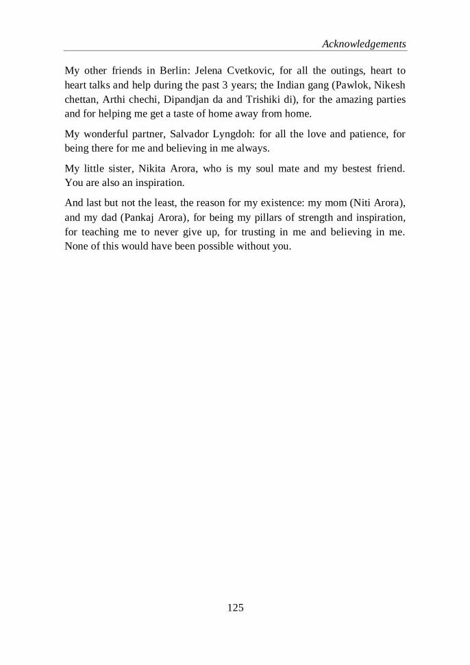
Acknowledgements
125
My other friends in Berlin: Jelena Cvetkovic, for all the outings, heart to
heart talks and help during the past 3 years; the Indian gang (Pawlok, Nikesh
chettan, Arthi chechi, Dipandjan da and Trishiki di), for the amazing parties
and for helping me get a taste of home away from home.
My wonderful partner, Salvador Lyngdoh: for all the love and patience, for
being there for me and believing in me always.
My little sister, Nikita Arora, who is my soul mate and my bestest friend.
You are also an inspiration.
And last but not the least, the reason for my existence: my mom (Niti Arora),
and my dad (Pankaj Arora), for being my pillars of strength and inspiration,
for teaching me to never give up, for trusting in me and believing in me.
None of this would have been possible without you.
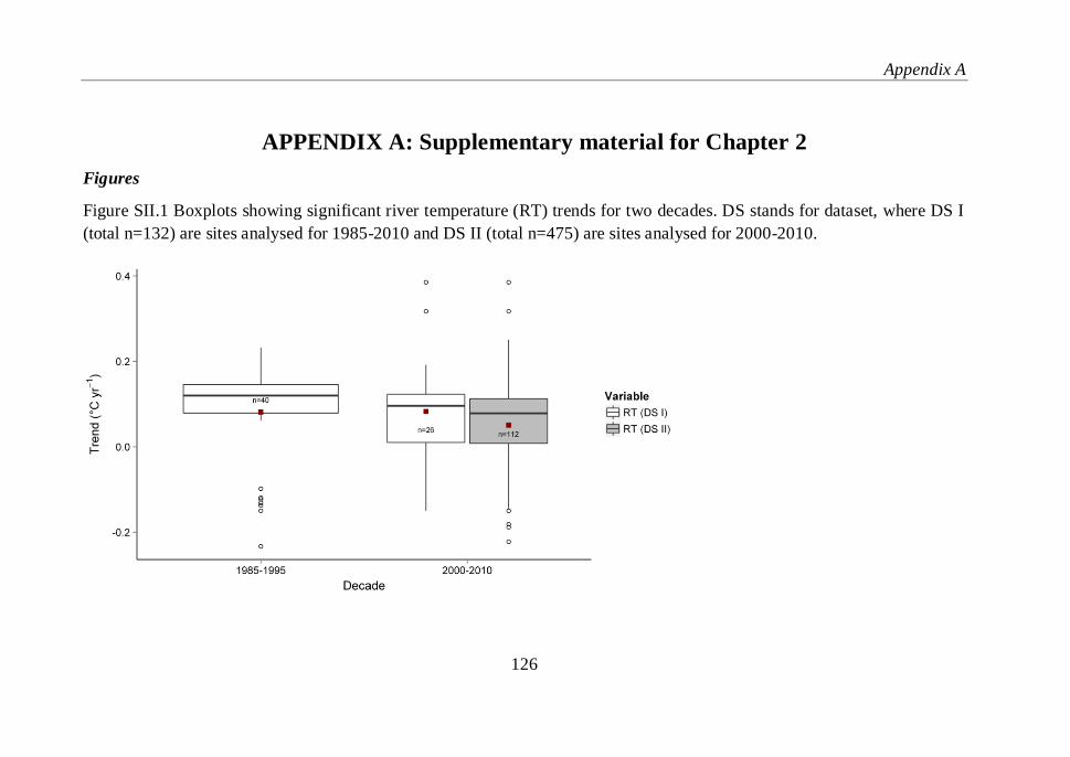
Appendix A
126
APPENDIX A: Supplementary material for Chapter 2
Figures
Figure SII.1 Boxplots showing significant river temperature (RT) trends for two decades. DS stands for dataset, where DS I
(total n=132) are sites analysed for 1985-2010 and DS II (total n=475) are sites analysed for 2000-2010.

Appendix A
127
Figure SII.2 Cumulative frequency distribution (ecdf) for proportion of forest, agriculture and urban land use cover types
within 1 km2 site buffers (time period:2000-2010; n=112).
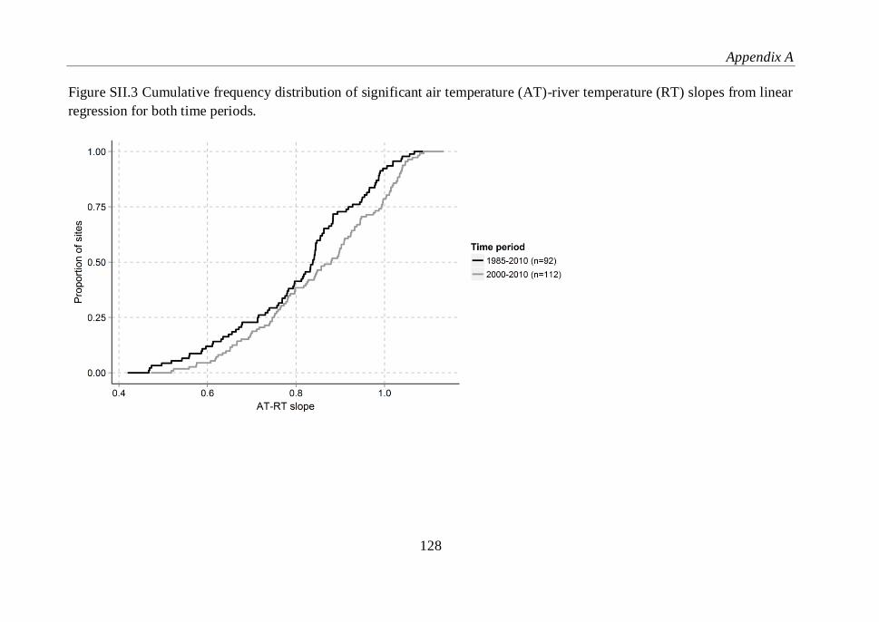
Appendix A
128
Figure SII.3 Cumulative frequency distribution of significant air temperature (AT)-river temperature (RT) slopes from linear
regression for both time periods.
Appendix A
129
Figure SII.4 Frequency of months with mean monthly river temperature above the threshold temperature of 22°C plotted for
several sites. The threshold temperature was based on thermal limits of fish and invertebrate species as mentioned in
Hardewig et al. (2004), Haidekker & Hering (2008) and Vornanen et al. (2014).
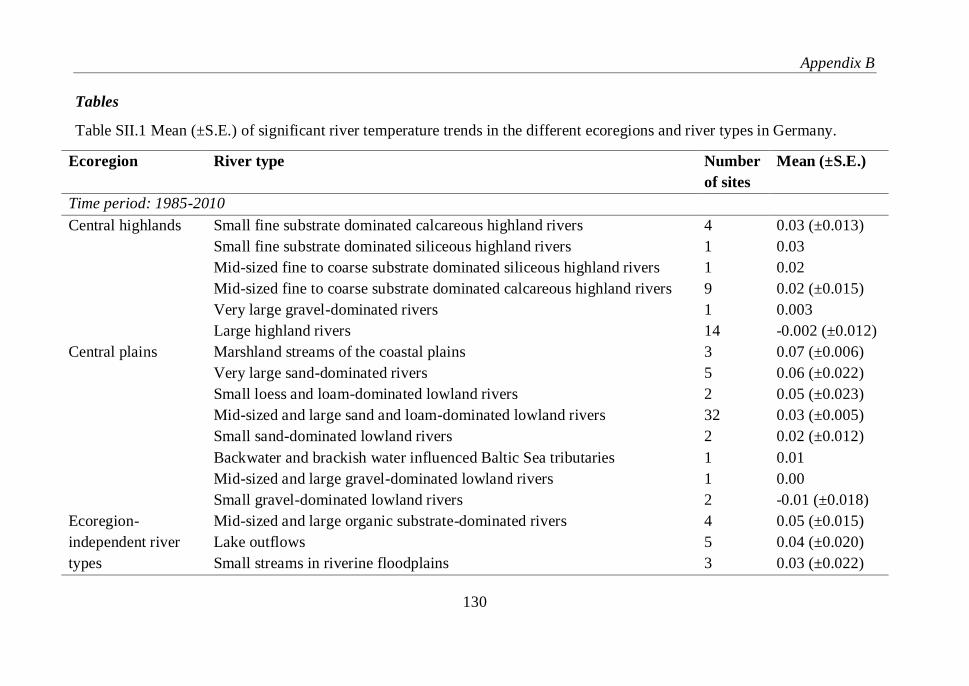
Appendix B
130
Tables
Table SII.1 Mean (±S.E.) of significant river temperature trends in the different ecoregions and river types in Germany.
Ecoregion River type Number
of sites
Mean (±S.E.)
Time period: 1985-2010
Central highlands
Small fine substrate dominated calcareous highland rivers 4 0.03 (±0.013)
Small fine substrate dominated siliceous highland rivers 1 0.03
Mid-sized fine to coarse substrate dominated siliceous highland rivers 1 0.02
Mid-sized fine to coarse substrate dominated calcareous highland rivers 9 0.02 (±0.015)
Very large gravel-dominated rivers 1 0.003
Large highland rivers 14 -0.002 (±0.012)
Central plains
Marshland streams of the coastal plains 3 0.07 (±0.006)
Very large sand-dominated rivers 5 0.06 (±0.022)
Small loess and loam-dominated lowland rivers 2 0.05 (±0.023)
Mid-sized and large sand and loam-dominated lowland rivers 32 0.03 (±0.005)
Small sand-dominated lowland rivers 2 0.02 (±0.012)
Backwater and brackish water influenced Baltic Sea tributaries 1 0.01
Mid-sized and large gravel-dominated lowland rivers 1 0.00
Small gravel-dominated lowland rivers 2 -0.01 (±0.018)
Ecoregion-
independent river
types
Mid-sized and large organic substrate-dominated rivers 4 0.05 (±0.015)
Lake outflows 5 0.04 (±0.020)
Small streams in riverine floodplains 3 0.03 (±0.022)
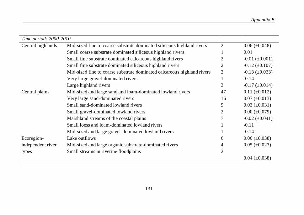
Appendix B
131
Time period: 2000-2010
Central highlands
Mid-sized fine to coarse substrate dominated siliceous highland rivers 2 0.06 (±0.048)
Small coarse substrate dominated siliceous highland rivers 1 0.01
Small fine substrate dominated calcareous highland rivers 2 -0.01 (±0.001)
Small fine substrate dominated siliceous highland rivers 2 -0.12 (±0.107)
Mid-sized fine to coarse substrate dominated calcareous highland rivers 2 -0.13 (±0.023)
Very large gravel-dominated rivers 1 -0.14
Large highland rivers 3 -0.17 (±0.014)
Central plains
Mid-sized and large sand and loam-dominated lowland rivers 47 0.11 (±0.012)
Very large sand-dominated rivers 16 0.07 (±0.013)
Small sand-dominated lowland rivers 9 0.03 (±0.031)
Small gravel-dominated lowland rivers 2 0.00 (±0.079)
Marshland streams of the coastal plains 7 -0.02 (±0.041)
Small loess and loam-dominated lowland rivers 1 -0.11
Mid-sized and large gravel-dominated lowland rivers 1 -0.14
Ecoregion-
independent river
types
Lake outflows 6 0.06 (±0.038)
Mid-sized and large organic substrate-dominated rivers 4 0.05 (±0.023)
Small streams in riverine floodplains 2
0.04 (±0.038)
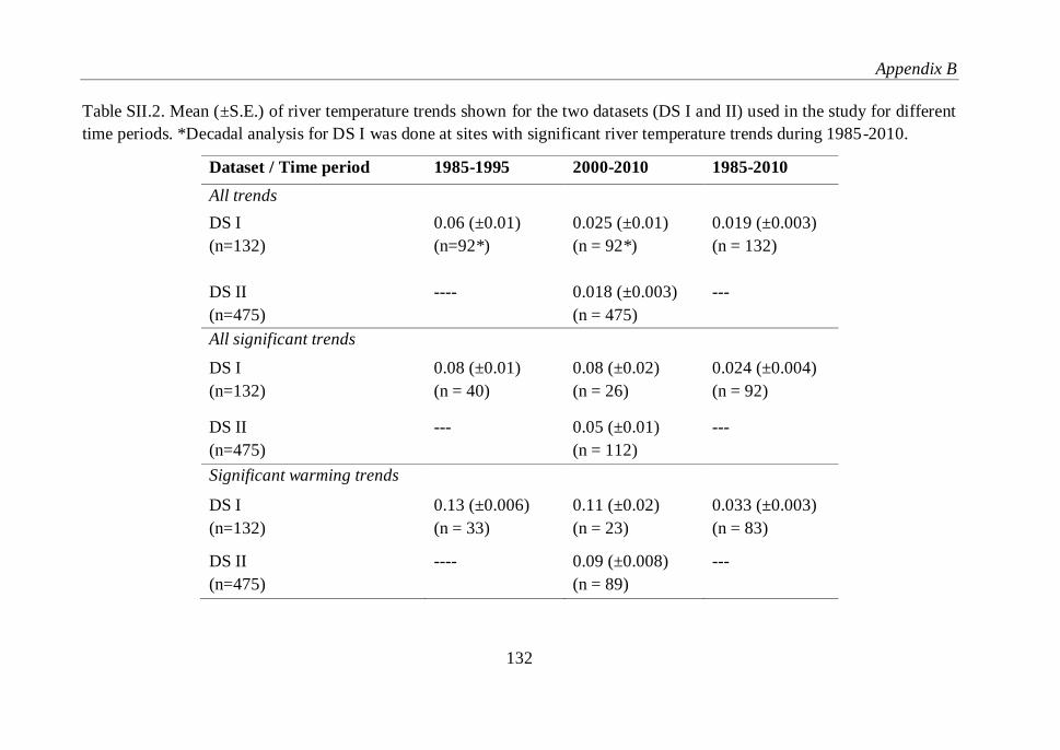
Appendix B
132
Table SII.2. Mean (±S.E.) of river temperature trends shown for the two datasets (DS I and II) used in the study for different
time periods. *Decadal analysis for DS I was done at sites with significant river temperature trends during 1985-2010.
Dataset / Time period 1985-1995 2000-2010 1985-2010
All trends
DS I
(n=132)
0.06 (±0.01)
(n=92*)
0.025 (±0.01)
(n = 92*)
0.019 (±0.003)
(n = 132)
DS II
(n=475)
---- 0.018 (±0.003)
(n = 475)
---
All significant trends
DS I
(n=132)
0.08 (±0.01)
(n = 40)
0.08 (±0.02)
(n = 26)
0.024 (±0.004)
(n = 92)
DS II
(n=475)
--- 0.05 (±0.01)
(n = 112)
---
Significant warming trends
DS I
(n=132)
0.13 (±0.006)
(n = 33)
0.11 (±0.02)
(n = 23)
0.033 (±0.003)
(n = 83)
DS II
(n=475)
---- 0.09 (±0.008)
(n = 89)
---
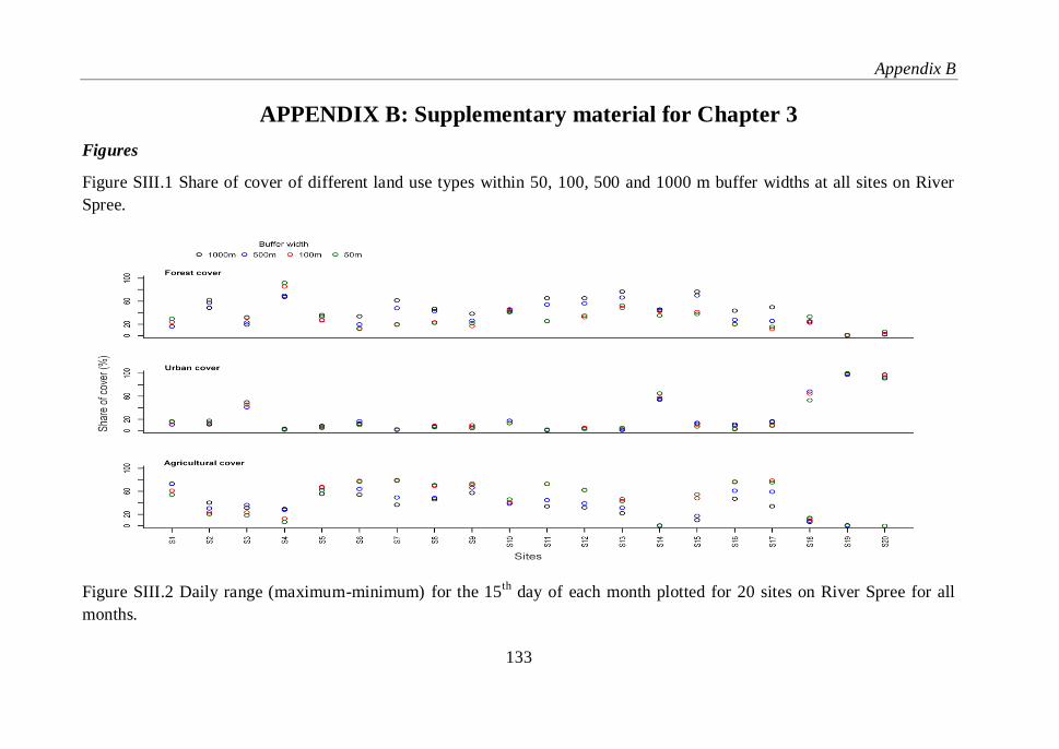
Appendix B
133
APPENDIX B: Supplementary material for Chapter 3
Figures
Figure SIII.1 Share of cover of different land use types within 50, 100, 500 and 1000 m buffer widths at all sites on River
Spree.
Figure SIII.2 Daily range (maximum-minimum) for the 15th
day of each month plotted for 20 sites on River Spree for all
months.
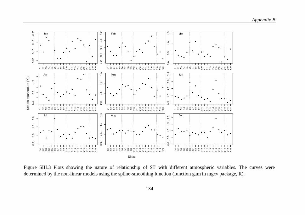
Appendix B
134
Figure SIII.3 Plots showing the nature of relationship of ST with different atmospheric variables. The curves were
determined by the non-linear models using the spline-smoothing function (function gam in mgcv package, R).
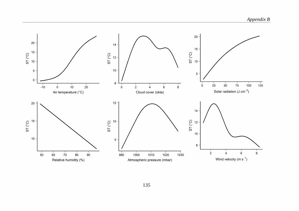
Appendix B
135
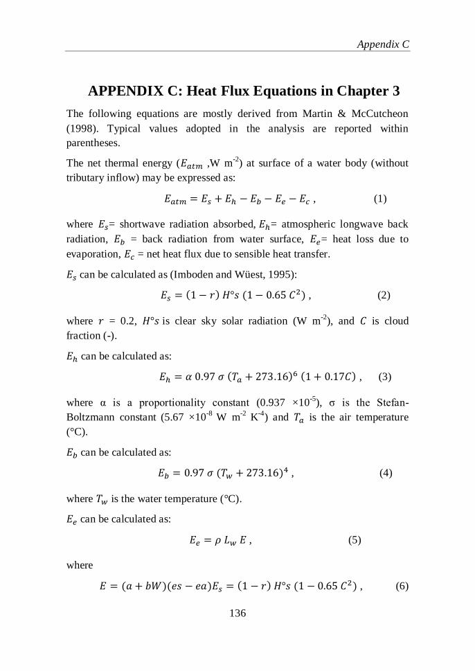
Appendix C
136
APPENDIX C: Heat Flux Equations in Chapter 3
The following equations are mostly derived from Martin & McCutcheon
(1998). Typical values adopted in the analysis are reported within
parentheses.
The net thermal energy (𝐸𝑎𝑡𝑚 ,W m-2
) at surface of a water body (without
tributary inflow) may be expressed as:
𝐸𝑎𝑡𝑚 = 𝐸𝑠 + 𝐸ℎ − 𝐸𝑏 − 𝐸𝑒 − 𝐸𝑐 , (1)
where 𝐸𝑠= shortwave radiation absorbed, 𝐸ℎ= atmospheric longwave back
radiation, 𝐸𝑏 = back radiation from water surface, 𝐸𝑒= heat loss due to
evaporation, 𝐸𝑐 = net heat flux due to sensible heat transfer.
𝐸𝑠 can be calculated as (Imboden and Wüest, 1995):
𝐸𝑠 = (1 − 𝑟) 𝐻°𝑠 (1 − 0.65 𝐶2) , (2)
where 𝑟 = 0.2, 𝐻°𝑠 is clear sky solar radiation (W m-2
), and 𝐶 is cloud
fraction (-).
𝐸ℎ can be calculated as:
𝐸ℎ = 𝛼 0.97 𝜎 (𝑇𝑎 + 273.16)6 (1 + 0.17𝐶) , (3)
where α is a proportionality constant (0.937 ×10⁻⁵
), σ is the Stefan-
Boltzmann constant (5.67 ×10⁻⁸
W m-2
K-4
) and 𝑇𝑎 is the air temperature
(°C).
𝐸𝑏 can be calculated as:
𝐸𝑏 = 0.97 𝜎 (𝑇𝑤 + 273.16)4 , (4)
where 𝑇𝑤 is the water temperature (°C).
𝐸𝑒 can be calculated as:
𝐸𝑒 = 𝜌 𝐿𝑤 𝐸 , (5)
where
𝐸 = (𝑎 + 𝑏𝑊)(𝑒𝑠 − 𝑒𝑎)𝐸𝑠 = (1 − 𝑟) 𝐻°𝑠 (1 − 0.65 𝐶2) , (6)
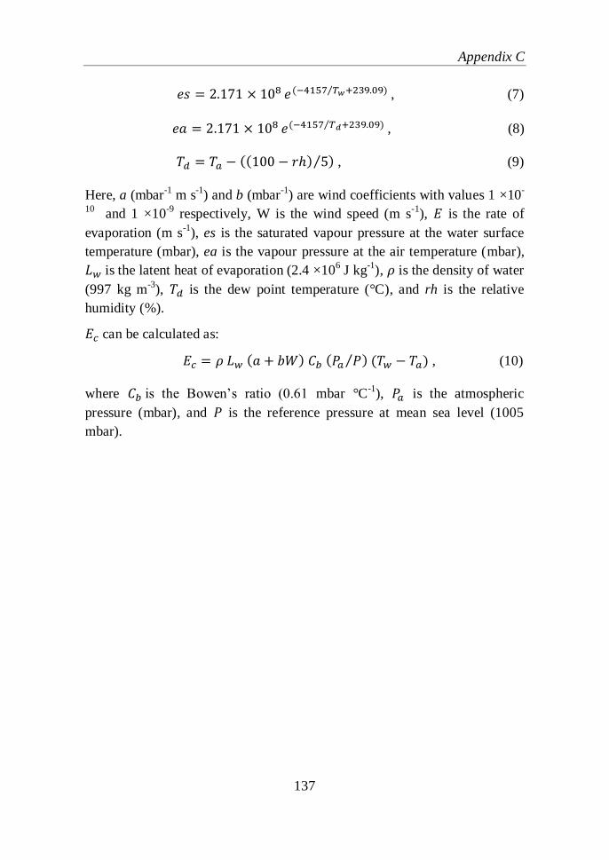
Appendix C
137
𝑒𝑠 = 2.171 × 10⁸ 𝑒(−4157 𝑇𝑤+239.09)⁄ , (7)
𝑒𝑎 = 2.171 × 10⁸ 𝑒(−4157 𝑇𝑑+239.09)⁄ , (8)
𝑇𝑑 = 𝑇𝑎 − ((100 − 𝑟ℎ) 5⁄ ) , (9)
Here, a (mbar-1
m s-1
) and b (mbar-1
) are wind coefficients with values 1 ×10-
10 and 1 ×10
-9 respectively, W is the wind speed (m s
-1), 𝐸 is the rate of
evaporation (m s-1
), es is the saturated vapour pressure at the water surface
temperature (mbar), ea is the vapour pressure at the air temperature (mbar),
𝐿𝑤 is the latent heat of evaporation (2.4 ×10⁶ J kg
-1), 𝜌 is the density of water
(997 kg m-3
), 𝑇𝑑 is the dew point temperature (°C), and rh is the relative
humidity (%).
𝐸𝑐 can be calculated as:
𝐸𝑐 = 𝜌 𝐿𝑤 (𝑎 + 𝑏𝑊) 𝐶𝑏 (𝑃𝑎 𝑃⁄ ) (𝑇𝑤 − 𝑇𝑎) , (10)
where 𝐶𝑏 is the Bowen’s ratio (0.61 mbar °C-1
), 𝑃𝑎 is the atmospheric
pressure (mbar), and 𝑃 is the reference pressure at mean sea level (1005
mbar).