rivers and streams - thayer school of engineeringd30345d/books/efm/...although there is no precise...

Chapter 15

Rivers and Streams

SUMMARY: Rivers are, in first approximation, nearly one-dimensional flows drivenby gravity down a slope and resisted by friction. While this may seem simple froma physical perspective, nonlinearities in the dynamics engender complex behavior.After a description of the basic hydraulic regimes, the chapter addresses water-qualityissues.

15.1 Open Channel Flow

Introduction

Streams and rivers form an essential link in the hydrological cycle and, in thatcapacity, provide freshwater for consumption and irrigation. Through their watershed,they also gather, convey and disperse almost any substance that enters water on land.Streams and rivers are thus central actors of environmental transport and fate.

Rivers and streams are types of open channels, i.e., conduits of water with a freesurface. In contrast to canals, ditches, aquaducts and other structures designed andbuilt by humans, rivers and streams are the products of natural geological processesand, as a consequence, are quite irregular. They have the ability to scour their beds,carry sediments and deposit these sediments, forever altering their own channels.Although there is no precise distinction made between rivers and streams, streams(Figure 15.1) are smaller and more rugged, their depth is shallow, and their watersgenerally flow faster, whereas rivers (Figure 15.2) are deeper, wider and more tran-quil. As we shall see, open-channel dynamics, called hydraulics, allow for two ratheropposite types of motion, one shallow and fast (supercritical) and the other deep andslow (subcritical). However, it would be unwise to charaterize streams by one typeand rivers by the other, because the same channel may exhibit varying properties

115

116 CHAPTER 15. RIVERS & STREAMS

Figure 15.1: A small stream inVermont, USA. [Photo by theauthor]

Figure 15.2: The Connecticut River at the level of Hanover, New Hampshire, USA.[Photo by the author]

15.1. OPEN CHANNEL FLOW 117

along its downstream path that make the water alternatively pass from one regimeto the other. This is often the case when the bottom slope is irregular.

In a first step, we establish the equations governing the water velocity and waterdepth as functions of the downstream distance and time, with particular attentionpaid to the case of a rectangular channel bed. Then, we consider a series of particularcases of interest: steady and unsteady flow, gradually and rapidly varying in thedownstream direction.

Equations of motion

River flow is actually three-dimensional because the velocity depends not only ondownstream distance but also on depth and transverse position. This is so becausefriction against the bottom and banks causes the velocity to decrease from a maximumat the surface near the middle of the stream to zero along the bottom and sides. Inaddition, centrifugal effects in river bends generate secondary circulations that renderthe velocity a full three-dimensional vector.

Because we wish to emphasize here the manner by which the flow varies in thedownstream direction, we will neglect cross-stream velocity components as well ascross-stream variations of the downstream component, by considering the speed u asthe water velocity averaged across the stream and a function of only the downstreamdistance x and time t. Because the flow in a river almost never reverses, the fact thatwe take x directed downstream implies that u is a positive quantity.

With a free surface exposed to the atmosphere, the water depth in a river can,too, vary in space and time. This implicates a second flow variable, namely the waterdepth, which we denote h and take as function of x and t, like the velocity. And likeu, h must be positive everywhere. The existence of two dependent variables, u(x, t)and h(x, t), calls for two governing equations. Naturally, these are statements of massconservation and momentum budget.

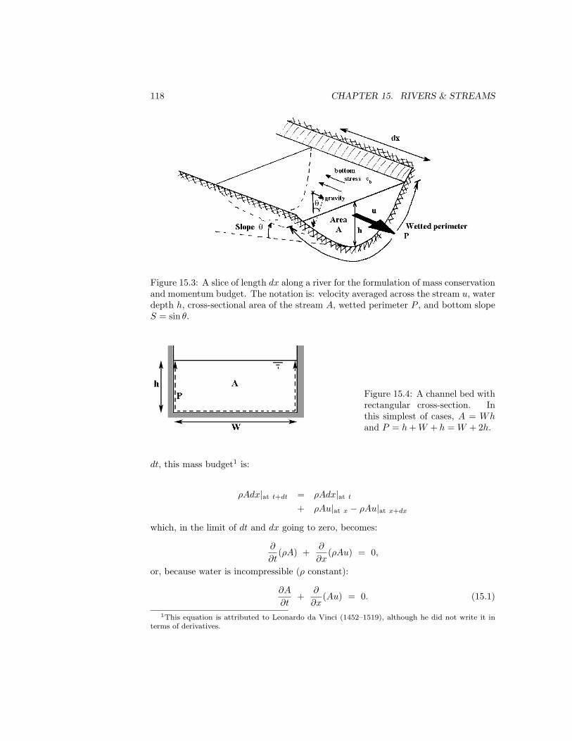
To establish the pair of governing equations, consider a slice of river as depictedin Figure 15.3. Geometric quantities are: A the cross-sectional area occupied by thewater, P the wetted perimeter (shortest underwater distance from bank to oppositebank following the curved bottom), S = sin θ the bottom slope, and h the waterdepth at the deepest point. The cross-sectional area A and wetted perimeter P areeach a function of the water depth h, because as h rises A and P increase in a waythat depends on the shape of the channel bed. For example, a channel bed withrectangular cross-section of width W (Figure 15.4) yields A = Wh and P = W + 2h.

Mass conservation

Conservation of mass is relatively straightforward. We simply need to state thatthe accumulation over time of mass ρAdx inside the slice of length dx is caused by apossible difference between the amount of mass ρAu that enters per time at positionx and the amount that leaves per time at position x + dx. For a short time interval


Figure 15.3: A slice of length dx along a river for the formulation of mass conservationand momentum budget. The notation is: velocity averaged across the stream u, waterdepth h, cross-sectional area of the stream A, wetted perimeter P , and bottom slopeS = sin θ.

Figure 15.4: A channel bed withrectangular cross-section. Inthis simplest of cases, A = Whand P = h+W + h = W + 2h.

dt, this mass budget1 is:

ρAdx|at t+dt = ρAdx|at t

+ ρAu|at x − ρAu|at x+dx

which, in the limit of dt and dx going to zero, becomes:

∂

∂t(ρA) +

∂

∂x(ρAu) = 0,

or, because water is incompressible (ρ constant):

∂A

∂t+

∂

∂x(Au) = 0. (15.1)

1This equation is attributed to Leonardo da Vinci (1452–1519), although he did not write it interms of derivatives.


Since the manner in which the cross-sectional area A increases with the waterdepth h is known from the shape of the channel bed, the preceding equation actuallygoverns the temporal evolution of the water depth h. It requires the knowledge ofthe velocity u, for which a second equation is necessary. This will be fulfilled once wehave established the momentum budget.

In the meantime, it is instructive to write the mass-conservation equation in thecase of a rectangular cross-section of constant width. With A = Wh, Equation (15.1)reduces to:

∂h

∂t+

∂

∂x(hu) = 0. (15.2)

Momentum budget

We write that the time rate of change of momentum inside our slice of river is themomentum flux entering upstream, minus the momentum flux exiting downstream,plus the sum of accelerating forces (acting in the direction of the flow), and minusthe sum of the decelerating forces (acting against the flow). Symbolically:

d

dt[Momentum inside the slice] = Momentum flux entering at x

− Momentum flux exiting at x+ dx

+ Pressure force in the rear

− Pressure force ahead

+ Downslope gravitational force

− Frictional force along the bottom.

The momentum is the mass times the velocity, that is (ρdV )u = ρAudx, whereasthe momentum flux is the mass flux times the velocity, that is (ρAu)u = ρAu2. Thepressure force Fp at each end of the slice is obtained from the integration of thedepth-dependent pressure over the cross-section:

Pressure force = Fp =

∫∫

pdA =

∫ h

0

p(z)w(z)dz,

in which p(z) and w(z) are, respectively, the pressure and channel width at levelz, with z varying from zero at the bottom-most point to h at the surface. Underthe assumption of a hydrostatic balance, the pressure increases linearly with depthaccording to

p(z) = ρg(h− z), (15.3)

discounting the atmospheric pressure which acts all around and has no net effect onthe flow. The pressure force is thus equal to:

Fp =

∫ h

0

ρg(h− z)w(z)dz, (15.4)


and is a function of how filled the channel is. In other words, it is a function of depthh. Taking the h derivative (which will be needed later), we have:

dFh

dh= [ρg(z − h)w(z)]z=h +

∫ h

0

ρgw(z)dz

= ρg

∫ h

0

w(z)dz = ρgA. (15.5)

The gravitational force is the weight of the water slice projected along the x–direction, which is mg times the sine of the slope angle θ:

Gravitational force = [(ρdV )g] sin θ = ρgASdx. (15.6)

Finally, the frictional force is the bottom stress τb multiplied by the wetted surfacearea:

Frictional force = τbPdx. (15.7)

River flows are typically in a state of turbulence and, within a certain level of approx-imation, the bottom stress is proportional to the square of the velocity. Invoking adrag coefficient CD, we write:

Bottom stress = τb = CDρu2, (15.8)

which resembles a Reynolds stress (τ = −ρu′w′, with the turbulent fluctuations u′

and w′ each proportional to the average velocity u). The frictional force exerted onthe slice of water is then:

Frictional force = τbPdx = CDρPu2dx. (15.9)

Values for the drag coefficient in rivers vary between 0.003 and 0.02, but there is nouniversal value for a given channel bed because CD varies with the Reynolds numberof the flow as well as with the shape and roughness of the channel bed. For the sakeof mathematical simplicity, however, we do not enter into those details right away.

We now gather the pieces of the momentum budget:

[ρAudx|at t+dt − ρAudx|at t]

dt= ρAu2|at x − ρAu2|at x+dx

+ Fp|at x − Fp|at x+dx

+ ρgASdx

− CDρPu2dx,

or, in differential form,

∂

∂t(ρAu) +

∂

∂x(ρAu2) = − ∂Fp

∂x+ ρgAS − CDρPu2.


Using the mass-conservation equation (15.1), we can reduce the left-hand side ofthis equation. Then, thanks to (15.5), the gradient of the pressure force becomes

∂Fp

∂x=

dFp

dh

∂h

∂x= ρgA

∂h

∂x.

A division by ρA finally yields:

∂u

∂t+ u

∂u

∂x= − g

∂h

∂x+ gS − CD

u2

Rh. (15.10)

In this equation the ratio of the cross-sectional area A over the wetted perimeter P ,which has the dimension of a length, was defined as

Rh =A

P. (15.11)

This is called the hydraulic radius. Because most rivers are much wider than they aredeep, the wetted perimeter is generally not much more than the width (P ≃ W ), andthe hydraulic radius is approximately the average depth h, which itself is not verydifferent from the center depth if the channel has a broad flat bottom, as is often thecase with natural streams:

Rh ≃ A

W= h ≃ h. (15.12)

The average depth h is exactly equal to the maximum depth h for a rectangularcross-section (Figure 15.4).

In Equation (15.10), the quantity Rh is a function of the water depth h. Themomentum equation, therefore, establishes a new relation between the velocity uand depth h, which together with mass conservation (15.1) forms a closed set of twoequations for two unknowns.

Because each equation contains a first-order derivative in time and also one inspace, the system is of second order in both time and space. Two initial conditionsand two boundary conditions are thus required to specify fully the problem. Theinitial conditions are naturally the spatial distribution of ho(x) and uo(x) at someoriginal time, but it is far less clear what the boundary conditions ought to be andwhere they should be applied. As we shall see, imposing an upstream value of h andan upstream value of u does not necessarily work.

For a wide channel with broad flat bottom or with a rectangular cross-section, Rh

may be replaced by h, and the momentum equation reduces to:

∂u

∂t+ u

∂u

∂x= − g

∂h

∂x+ gS − CD

u2

h. (15.13)

The pair (15.1)–(15.10) are called the Saint-Venant2 equations. Even in its sim-plified form, the set (15.2)–(15.13) for a wide rectangular channel is highly nonlinear.So, non-unique solutions and other surprises may occur.

2Adhemar de Saint-Venant (1797–1886), a French civil engineer who spent a significant part ofhis career working for the country’s Bridges and Highways Department


15.2 Uniform Frictional Flow

Our first particular case is that of a steady and uniform flow down a constant slope.With the temporal and spatial derivatives set to zero, Equation (15.1) is triviallysatisfied, while the momentum budget (15.10) reduces to:

CDu2

Rh= gS, (15.14)

which simply states that the downslope force of gravity is resisted entirely by bottomfriction. This is similar to a parachute in action, in which the downward force ofgravity, which is constant, is balanced by the upward force of air drag, which isproportional to the square of the velocity. The equation can be readily solved for thevelocity:

u =

√

gRhS

CD. (15.15)

This is known as the Chezy3 formula.For a wide channel with broad flat bottom, the hydraulic radius Rh is nearly the

water depth h, and (15.15) reduces to:

u =

√

ghS

CD. (15.16)

The formula (in either form) is physically correct but hides a complication insidethe drag coeffcient CD, which varies from river to river and with the water depth.Over the years, a number of improvements to the formula have been proposed torender the dependence on the water depth and bed roughness more explicit. We shallpresent only two here.

River flow falls in the category of shear turbulence. Thus, according to Section8.2, an appropriate representation of the velocity profile over depth is the logarithmicprofile:

u(z) =u∗

κln

z

zo, (15.17)

in which u∗ is the friction velocity (related to the stress against the boundary), κ thevon Karman constant, and zo the roughness height (a fraction of the mean height ofthe bottom asperities). As shown in Section 8.2, from this profile, one can obtain arelation between the bottom stress and the depth-averaged velocity u:

τb =ρκ2u2

[ln(h/zo)− 1]2. (15.18)

from which follows an expression for the drag coefficient:

3in honor of Antoine Leonard de Chezy (1718–1798), a French engineer who designed canals forsupplying water to the city of Paris

15.2. UNIFORM FLOW 123

CD =κ2

[ln(h/zo)− 1]2. (15.19)

It is clear from this expression that the drag coefficient depends on both the roughnessof the channel bed and the water depth. For κ = 0.41 and a height ratio h/zo in therange 30–2000, the drag coefficient varies between 0.004 and 0.03. Substituting in theChezy formula (15.16), we obtain:

u =

√

ghS

κ2

[

lnh

zo− 1

]

. (15.20)

Having abundant data at his disposal and looking for a power law, Manning4

determined that a 2/3 power was giving the best fit and proposed the followingformula, in terms of the hydraulic radius:

u =1

nR

2/3h S1/2 . (15.21)

This is not too surprising since for realistic values of h/zo (on the order of 1000), thebest power-law fit to the function ln(h/zo) − 1 is 1.87(h/zo)

1/6, turning (15.20) intoa 2/3 power of h.

In Equation(15.21), the coefficient n in the denominator is called the Manning

coefficient and its value depends on the roughness of the channel bed (Table 15.1).

Regardless of what is done with the drag coeffcient, Equation (15.15) remains validfrom basic physical principles. This gives the water velocity u in terms of the waterdepth h, and we may ask: How does a river select a specific value for u and a specificvalue for h water depth among the infinite possibilities offered by this functionalrelationship? The degree of freedom is set by the river’s volumetric flow rate, calledthe discharge and noted Q. With

Q = Au, (15.22)

Equations (15.15) and (15.22) form a two-by-two system of equations for h and u.The solution in the particular case of a wide rectangular channel (A = Wh and

Rh ≃ h) is:

h =

(

CDQ2

gSW 2

)

1

3

(15.23)

u =

(

gSQ

CDW

)1

3

. (15.24)

4Robert Manning (1816–1897), Irish engineer and surveyor. History reveals that he was the firstto propose a 2/3 power law.


Table 15.1: Values of the Manning coefficient for common channels

CHANNEL TYPE n

Artificial channels finished cement 0.012unfinished cement 0.014brick work 0.015rubble masonry 0.025smooth dirt 0.022gravel 0.025with weeds 0.030cobbles 0.035

Natural channels mountain streams 0.045clean and straight 0.030clean and winding 0.040with weeds and stones 0.045most rivers 0.035with deep pools 0.040irregular sides 0.045dense side growth 0.080

Flood plains farmland 0.035small brushes 0.125with trees 0.150

Because the water depth h varies like Q2/3 whereas the velocity u varies as Q1/3,we deduce that an increase in discharge generates a larger increase in depth than invelocity. So, when a flood condition arises, a river adapts by increasing its depthmore than its velocity. The interesting result, however, is that the two quantities areintimately related to each other. It is presumed that this is the reason why Romanengineers of antiquity were successful at conveying clean water by aquaducts andremoving waste water by sewers5.

When the flow is not uniform but gradually varying, because the slope is notconstant or there are other elements that activate the derivatives in (15.1) and (15.10),the value of h given by (15.23) is not necessarily the water depth realized by the streambut nonetheless serves as a useful reference against which the actual water depth maybe compared. In this case, it is called the normal depth and is denoted by hn:

hn =

(

CDQ2

gSW 2

)

1

3

. (15.25)

As we shall see later, the cases h < hn (flow is too thin and fast) and h > hn (theflow is too thick and slow) exhibit different dynamical properties.

5Indeed, Romans did not have a notion of time on the scale of the second and minute, only on thescale of hours and days by following the motion of the sun in the sky. As a consequence, they hadno concept of a velocity and only had at their disposal the water depth, which they could measurewith a stick. So, all their calculations were exclusively based on water depth, but the fact that h

and u are tightly related to each other allowed them to obtain practical estimates for the design oftheir water lines.

15.3. THE FROUDE NUMBER 125

15.3 The Froude Number

In what follows, a dimensionless ratio plays a crucial role. It is the so-called Froude

number, defined from the average velocity u and the average depth h as:

Fr =u

√

gh. (15.26)

Physically, it compares the actual water velocity to the speed of gravity waves on thesurface (traveling at speed

√gh in a shallow fluid of depth h, according to Section

4.1.5).Two cases arise. Either the water flows less fast than waves on its surface (u <

√

gh → Fr < 1) and the flow is said to be subcritical, or the water flows faster than

the waves on its surface u >√

gh → Fr > 1) and the flow is said to be supercritical.The flow is critical when its Froude number is unity.

The critical depth is the depth that a given discharge Q = Au adopts when theflow is critical. For a wide, rectangular channel (A = Wh and h = h), it is

hc =

(

Q2

gW 2

)

1

3

. (15.27)

A way of determining whether a flow is subcritical or supercritical is to compareits actual depth h to the critical depth hc for that flowrate: If h > hc, the flow issubcritical, while for h < hc the flow is supercritical.

15.4 Gradually Varied Flow

We now turn our attention to slowly varying flows, in which downstream variationsplay a role (∂/∂x 6= 0), but continue to restrict our attention to steady flows (∂/∂t =0). With the velocity obtained in terms of the water depth and discharge [u = Q/Aaccording to (15.22)], the momentum equation (15.10) becomes:

− Q2

A3

dA

dh

dh

dx+ g

dh

dx= gS − CD

Q2

RhA2,

which can be simplified by noting as earlier that dA/dh is the width W at the surface(see Figure 15.5). Furthermore, with A/W = h, the average depth, it becomes:

− Q2

A2h

dh

dx+ g

dh

dx= gS − CD

Q2

RhA2.

Now, gathering the dh/dx terms together and dividing by g, we obtain:

(

1 − Q2

gA2h

)

dh

dx= S − CDQ2

gRhA2. (15.28)


Figure 15.5: Relation be-tween cross-sectional area A,width W and water depth hin a non-rectangular channel.When the water depth risesincrementally by dh, the areaincreases by Wdh.

The fraction inside the parentheses on the left-hand side is equal to u2/gh and isthus the Froude number squared. The equation governing the downstream variationof water depth then takes the form:

(1 − Fr2)dh

dx= S

(

1 − CDQ2

gSRhA2

)

. (15.29)

As we can note, it is not a priori clear whether the depth increases (dh/dx > 0)or decreases (dh/dx < 0) in the downstream direction, because each parentheticalexpression can be either positive or negative. A number of possibilities arise, whichwe shall discuss them in the simpler case of a wide rectangular channel.

Wide rectangular channel

When the river channel is wide and rectangular, the average depth h and maximumdepth h are the same, the cross-sectional area A is Wh, the wetted perimeter P isnearly the width W , making the hydraulic radius Rh = A/P nearly equal to the waterdepth. With these simplifications, the preceding equation (15.29) becomes:

(

1 − Q2

gW 2h3

)

dh

dx= S

(

1 − CDQ2

gSW 2h3

)

,

or

(

1 − h3c

h3

)

dh

dx= S

(

1 − h3n

h3

)

, (15.30)

where hc and hn are respectively the critical and normal depths [see (15.27) and(15.25)]:

hc =

(

Q2

gW 2

)

1

3

and hn =

(

CDQ2

gSW 2

)

1

3

. (15.31)

Because the drag coefficient CD depends, although weakly, on the water depthh, according to (15.19) or some other formula proposed by various authors, the de-pendence of right-hand side of (15.30) on the variable h is more complicated than itappears. Nonetheless, the sign of the right-hand side is determined by comparing the

15.4. GRADUALLY VARIED FLOW 127

Figure 15.6: The profiles of the water surface in the eight possible cases of graduallyvaried flow.

actual water depth h value with the normal depth hn, whatever its exact value maybe.

We also note that, because hn depends on h (via CD) but hc does not, there cannotexist a situation in which hn and hc are equal to each other over any finite distance x.Indeed, if such were the case, Equation (15.30) would reduce to dh/dx = S, yieldingh(x) = Sx+constant, which makes h not constant and with it CD and hn. In otherwords, the case hn = hc cannot arise and needs not be considered.

Various possible cases

Equation (15.30) can be cast as

dh

dx= S

h3 − h3n

h3 − h3c

, (15.32)

which shows that the sign of dh/dx depends on how the actual water depth h comparesto both the critical and normal depths, hc and hn.

The bottom slope S is usually positive as rivers flow downhill. However, there arecases when the slope may be locally negative, forcing the water to flow over a risingbottom. A prime example is the overflow from a lake, in which the water flows froma deeper basin over a sill and then down along a river channel. In the case of anadverse slope, the parameter S is negative and with it the normal depth hn. Withthis in mind, the following cases can arise: The normal depth hn can be (1) negative,(2) positive and less than the critical depth hc, or (3) positive and greater than hc.For hn to exceed hc, the channel slope S must be sufficiently weak, namely

S < CD. (15.33)

In such case, the slope is said to be mild. In the contrary case, when (15.33) is notsatisfied, the slope is said to be steep, and hn falls below hc.

And, for every one of these cases, the actual water depth h may lie in any intervaldefined by 0, hc and hn, if the latter is positive. This leads to the following set ofeight possible cases:


Adverse slope (S < 0, hn < 0 < hc):A1: 0 < h < hc

A2: hc < hMild slope (S > 0, 0 < hc < hn):

M1: 0 < h < hc

M2: hc < h < hn

M3: hn < hSteep slope (S > 0, 0 < hn < hc):

S1: 0 < h < hn

S2: hn < h < hc

S3: hc < h

It is straightforward to note that dh/dx is positive in the following 5 cases: A1,M1, M3, S1, S3, and negative in the 3 others: A2, M2, S2. Next, we note that whenh approaches hn it does so asymptotically (cases S1 and S2), but when it approacheshc it does so in a singular way (dh/dx approaching infinity, cases A1, A2, M1 andM2). Finally, when h increases without bound (cases M3 and S3), Equation (15.32)yields dh/dx → S, implying that the rise in water depth compensates for the dropin bottom, and the water surface becomes horizontal. The water profile in the eightcases is displayed in Figure 15.6.

The behavior of the water level in some of the cases displayed in Figure 15.6 appearto be quite odd at first glance, because they lead to a singularity (dh/dx → ∞), butthey make sense in combinations with one another, as shown in Figure 15.7.

15.5 Lake Discharge Problem

A practical problem in hydraulics is the determination of the discharge (volumetricflow rate) from a lake given its water level and the slope of the exit channel. Twocases are possible: Either the slope of the exit channel is mild or steep. The selectionreduces to finding whether the channel slope S falls below or exceeds the value ofthe drag coefficient [see Inequality (15.33)] Since, the drag coefficient CD in the exitchannel is dependent on the water depth h and since the latter is not known until thedischarge is determined, the solution must proceed by trial and errors. But, let usassume here that we have made a reasonable guess about the value of CD and thatwe therefore know whether the slope of the exit channel is mild or steep.

The easier of the two cases is that of an exit channel with a steep slope (S > CD).The flow in the stream draining the lake is then of type S1, S2 or S3. By virtueof Figure 15.6, it is clear that we can reject S3, because the lake is upstream, notdownstream. The flow in the stream is therefore supercritical. And, of S1 and S2, itis quite clear that we need to select S2 because the flow goes from being deeper in thelake to shallower in the stream. The water velocity is virtually nil in the deep lake,and the Froude number there is nearly zero. Thus, the lake flow approaching the exit

15.5. LAKE DISCHARGE 129

Figure 15.7: Combinations of gradually-varied flows: (a) stream passing from a mildto a milder slope; (b) change from a steep to a steeper slope; (c) change from a mild toa steep slope; (d) lake discharging in a river with steep slope; (e) lake discharging in ariver with mild slope, which becomes steep further downstream; (f) lake dischargingin a river with mild slope, which runs into another lake. [Adapted from Sturm, 2001]


is subcritical. As the flow needs to pass from subcritical in the lake to supercriticalin the stream, it crosses criticality (h = hc) at the transition from the lake to thestream, that is, at the sill point (highest bottom point), as indicated in Figure 15.7d,and the sill exerts control.

Generally, the bottom rises abruptly in the lake in the vicinity of the sill point,and we can consider the portion of the flow on the lake side of the sill as rapidly varied(frictionless). The Bernoulli principle holds, telling us that the sum u2/2 + g(h + b)is constant from the deep lake to the sill. On the deep side, u ≃ 0 whereas h + b isequal to H, the elevation of the water surface in the lake above the height of the sill(see Figure 15.7d, with the datum taken as the sill level). At the sill, the velocity iscritical, u =

√gh (Fr = 1), whereas b is zero. Conservation of the Bernoulli function

then provides:

0

2+ gH =

gh

2+ gh,

which yields

h =2

3H, (15.34)

at the sill and, in turn,

u =√

gh =

√

2

3gH , (15.35)

at the sill, too. The discharge Q is the product Whu, where W is the channel width.The answer to the problem is thus:

Q = Whu =

(

2

3

)3/2

WH√

gH = 0.544 WH√

gH . (15.36)

The case of an exit channel with mild slope (S < CD) is somewhat more compli-cated. Rejecting immediately type M1, because the lake is upstream and not down-stream, we are left with a choice between flow types M2 and M3, each with controlat the downstream end of the channel, that is, away from the lake. If we can assumethat the channel is relatively long, then the flow at the head of the channel is theupstream asymptotic behavior of either M2 or M3, (as depicted in Figure 15.7e and15.7f). Thus, we are brought to conclude that the water depth reaches the normalvalue (h = hn) at the head of the channel. Assuming as in the case of a steep slopethat the lake flow approaching the sill varies rapidly from rest, we can again applythe Bernoulli principle and write:

0

2+ gH =

u2

2+ ghn,

which yields the velocity at the sill point:

u =√

2g(H − hn) . (15.37)

15.6. RAPIDLY VARIED FLOW 131

In terms of the discharge Q, the normal water depth is hn = (CDQ2/gSW 2)1/3 andthe corresponding water velocity is u = Q/Whn = (gSQ/CDW )1/3. Using these in(15.37) yields the value of Q:

Q =

[

1

2

(

S

CD

)2/3

+

(

CD

S

)1/3]

−3/2

WH√

gH , (15.38)

which reverts to (15.36) when S = CD, providing continuity between the two cases ofmild and steep slopes.

If the channel draining the lake does not preserve its mild slope for a long distance,then one needs to start from the end point of this channel stretch where control isoccurs and integrate in the upstream direction all the way to the sill. This is quitecomplicated because numerical integration requires a value for Q, which is not yetknown. One has therefore to proceed by successive trials until u2/2 + gh equals gHat the sill, to establish connection with the lake.

15.6 Rapidly Varied Flow

Bernoulli principle

In considering rapidly varied flow, friction may be neglected and the drag coeffi-cient CD is set to zero. Equation (15.10) in steady state reduces to:

udu

dx+ g

dh

dx+ g

db

dx= 0,

in which we have introduced the elevation b(x) of the channel bottom, so that theslope is minus its gradient: S = −db/dx.

This can be integrated over distance to obtain the Bernoulli principle:

u2

2+ gh + gb = B = a constant. (15.39)

Elimination of the velocity u by virtue of conservation equation (15.22) of the flowrate Q yields

Q2

2A2+ gh + gb = B. (15.40)

This constitutes an algebraic equation for the water depth h since the cross-sectionalarea A is a function of h. Given a cross-sectional profile A(h) and bottom elevationb, we can in principle solve the equation for h and, as either or both of these twoproperties change in the downstream direction, so does the value of h.

For a channel of rectangular cross-section, A = Wh with W the channel width,Equation (15.40) becomes:


Figure 15.8: Water flowing down a weir, which is a type of rapidly varied flow. TheBernoulli principle may be applied between Points 1 and 2. [Photo c©Chanson 2000]

Q2

2W 2h2+ gh + gb = B. (15.41)

The parameters are the discharge Q, the channel width W , the bottom elevation b,and the level B of energy in the flow. For given values of these parameters, the waterdepth h can be calculated. The parameters Q and B are constants along the stream,but rapid changes can occur in the width W and bottom elevation b. The water depthh then adapts locally, and this is the essence of a rapidly varied flow.

Note that Equation (15.41) can be turned into a cubic polynomial, which mayhave one, two or three real roots. Whether any, some or all of the real roots arepositive, which is required for h to be physically realizable, needs to be investigated.

It is the tradition in civil engineering, of which hydraulics is a discipline, to usevariables that correspond to vertical distances, called heads. To this effect, Equations(15.39) and (15.41) are divided by g:

u2

2g+ h + b =

B

g(15.42)

Q2

2gW 2h2+ h + b =

B

g. (15.43)

The term u2/2g = Q2/2gW 2h2 is called the velocity head, whereas h and b are obvi-ously vertical heights, that of water above the bottom of the channel and that of thebottom of the channel above sea level, respectively.

Specific energy


Figure 15.9: Variation of spe-cific energy E with waterdepth. It is customary inthis type of plot to have halong the vertical axis becauseit corresponds to a verticallength.

If we consider two points along the flow (Figure 15.8), with Point 1 upstream ofPoint 2, Equation (15.43) requires

Q2

2gW 21 h

21

+ h1 =Q2

2gW 22 h

22

+ h2 + ∆b,

in which ∆b = b2 − b1 is the change in bottom elevation. From this expression, it isclear that the sum of the velocity head and water depth must change if there is anychange in channel elevation. In consequence, it is instructive to consider this sumof two terms, which was first introduced by Bakhmeteff (1932) and has come to becalled the specific energy. By definition therefore,

E =Q2

2gW 2h2+ h (15.44)

for a channel with discharge Q and rectangular cross-section of width W .We note the following interchange in E upon varying h: When one of the two

terms increases, the other necessarily decreases. The limits of h going to zero and toinfinity are both E → ∞, and since E is finite for finite values of h and is obviouslywell behaved, it follows that E reaches a minimum for some value of h (Figure 15.9).Setting to zero the derivative with respect to h, we obtain:

− Q2

gW 2h3+ 1 = 0,

of which the solution is

hc =

(

Q2

gW 2

)

1

3

, (15.45)


in which we recognized the critical depth [see (15.27). The minimum value of E isobtained by setting h = hc:

Emin =3

2

(

Q2

gW 2

)

1

3

=3hc

2. (15.46)

A plot of the function E(h) is provided in Figure 15.9. It is clear that thereexist two possible values for h when E exceeds its minimum, one when it is at itsmimimum, and none when it falls below its minimum. [There also exists another realh root but it is always negative and not included in the plot.] When the channelwidth W increases, both Emin and hc decrease, and the curve moves inward, beingsqueezed inside the wedge defined by the horizontal axis and the bissectrix (h = Eline), and when W decreases the curve moves away from the apex of the wedge.

The Froude number is

Fr =u√gh

=

√

Q2

gW 2h3=

(

hc

h

)3

2

. (15.47)

Therefore, the upper branch of E corresponds to subcritical flow (Fr < 1) and thelower branch to supercritical flow (Fr > 1). The minimum of E corresponds to acritical state (Fr = 1), and this is why hc is called the critical depth. For any valuehigher than Emin, there thus exist two states, one subcritical (thick and slow, calledfluvial) and one supercritical (thin and fast, called torrential), but no state is realizablewhen E falls below Emin.

Flow over a bump

Let us now consider what happens when the stream encounters a bump alongthe bottom, while its width remains unchanged. So, b is now a function of x whichincreases and then decreases. Equations (15.43) requires the specific energy to changeaccording to

E + b =B

g, (15.48)

in which B/g is a constant. Thus, E must decrease where b increases and vice versa.At the top of the bump, E is lower than what it was upstream by exactly the heightof the bump, say ∆b. If the bump is modest and the flow is subcritical upstream,the point on the specific-energy diagram (Figure 15.10a) slides downward, the flowbecomes thinner and a bit faster. Physically, the flow is constricted from below andmust accelerate to accommodate an unchanged flowrate. But, acceleration demandsa force, and the surface must fall somewhat so that the flow can slide downwards toaccelerate. Another way of understanding this is to realize that the increase in kineticenergy necessary to squeeze the flow above the bump can only be at the expense ofpotential energy, and, as the potential energy falls, so does the surface.

Note the positive feedback in the situation. The flow is squeezed from below by thebump and must simultaneously experience a squeeze from the top. This can obviously


Figure 15.10: The possible ways by which a free-surface flow adapts to a bottombump: (a) The bump is modest, and the flow remains subcritical all along, exhibitingonly a dip over the bump; (b) the bump is high, and the flow becomes critical at thetop of the bump and supercritical thereafter.

lead to a problem: If the bump is of sufficient height, the required drop in the surfacelevel might become excessive and intersect the raised bottom. This is what happenswhen the height of the bump exceeds the difference between the upstream value of Eand its minimum Emin. The value of E should fall below its minimum but this maynot happen. The flow cannot pass over the bump, at least not all of it. The flow issaid to be choked.

The situation becomes unsteady. Water arrives at the obstacle faster than itcan pass over it and accumulates. This accumulation in turn raises the water levelupstream, and, with it, the potential energy of the flow. Mathematically, the value ofthe Bernoulli function B is now augmenting, and with it the specific energy E of theflow upstream. This will continue until E has been raised just enough that the newdifference E − Emin above the minimum can match the height ∆b of the bump.

On the specific-energy diagram, the point slides down along the upper branch onthe climbing side of the bump and reaches the minimum at the top (Figure 15.10b).Downstream, the point does not proceed reversibly but keeps on sliding along the


Figure 15.11: The possible ways by which a free-surface flow passes through a narrow-ing section: (a) The narrowing is modest, and the flow remains subcritical all along,exhibiting only a dip in the constriction; (b) the narrowing is significant, and the flowbecomes critical at the narrowest section and supercritical thereafter.

lower branch of the curve. The flow has become thin and fast, that is, supercritical.The bump acts as a dam and spillway (see Figure 15.8 for example).

Both previous cases assumed that the oncoming flow was subcritical. Should itbe supercritical, again one of two things can happen. If the height of the bump ismodest, the flow slows down and thickens over the bump, because on the specificenergy diagram the point rises as it moves to the left and then relaxes. If the heightof the bump is large, the flow switches from being supercritical to subcritical. As itwill be shown later, however, supercritical flows are unstable and do not persist. Anapproaching supercritical flow is therefore quite unlikely.

Flow in a narrowing channel

Another way by which a flow can be choked and pass from subcritical to super-critical state is through a narrowing of the channel width. Now, b remains constantbut the width W of the channel experiences a local decrease, say from W upstream


and downstream to Wmin at the narrowest point (Figure 15.11). Since the bottomelevation b remains unchanged, the specific energy, too, remains constant by virtue of(15.48), but as the width W decreases, the specific-energy minimum (15.46) increasesand the curve in the E–h diagram moves to the right.

If the narrowing of the channel is modest (Figure 15.11a), the water depth dropssome as the channel narrows and recovers if the channel widens afterwards. But, if therestriction in channel cross-section is significant, then the flow undergoes a transitionfrom subcritical to supercritical state (assuming that it was subcritical upstream),with the critical point occurring at the narrowest cross-section (see Figure 15.11b).

Flooding

An interesting situation occurs when a river overflows its normal channel and spillsonto a broader floodplain. The floodplain naturally forms a new and wider channelbut the compounded cross-section of natural channel plus floodplain may no longerbe idealized as a channel of rectangular cross-section.

Consider a channel of arbitrary cross-section, for which the cross-sectional areaA(h) is some complicated function of the water depth h. The specific energy dependson h in the following general way:

E =Q2

2gA2(h)+ h, (15.49)

and reaches an extremum with respect to h when its derivative dE/dh vanishes, whichoccurs when:

1

A3(h)

dA

dh=

g

Q2.

As Figure 15.5 shows, the channel width at the surface is such that dA = Wdh andthus dA/dh = W . The preceding equation can therefore be expressed as:

A3(h)

W (h)=

Q2

g, (15.50)

which by virtue of its nonlinearity may admit more than one solution. If there is aunique solution, it must be a minimum since E tends to positive infinity when h goesto zero and to infinity. If (15.50) admits more than one root, then it is most likelythat the solutions come in a set of 3, 5 etc. (barring the exceptional cases of doubleroots). With three solutions, we expect two minima separated by one maximum.

Defining the averaged depth h as the cross-sectional area divided by the surfacewidth, namely

h =A

W, (15.51)

then (15.50) can be recast as


Figure 15.12: An idealized river channel and its floodplain. The river channel has awidth W and depth H, while the floodplain has a width W ′ significantly larger thanW .

A2h =Q2

g. (15.52)

If the Froude number is defined in terms of the averaged depth as

Fr =u

√

gh, (15.53)

then, using u = Q/A, we have

Fr =

√

Q2

gA2h, (15.54)

which reaches 1 whenever E reaches an extremum, as for the rectangular cross-section.

Channel with floodplain

A channel and its surrounding floodplain may be idealized as a wide and shallowrectangular channel with a deeper and narrower rectangular channel embedded withinit, as depicted in Figure 15.12.

In the non-flooding case h ≤ H, the cross-sectional area is A = Wh, the velocityu = Q/Wh, and the specific energy

E =Q2

2gW 2h2+ h,

whereas in the flooding case h > H, the cross-sectional area is A = WH+W ′(h−H)= W ′h−(W ′−W )H, the velocity u = Q/[W ′h−(W ′−W )H] and the specific energy

E =Q2

2g[W ′h− (W ′ −W )H]2+ h.

Extrema of E occur for


h =

(

Q2

gW 2

)

1

3

for h ≤ H

h =

(

Q2

gW ′2

)

1

3

+W ′ −W

W ′H for h > H,

and these are distinct roots if

(

Q2

gW 2

)

1

3

< H <

(

Q2

gW ′2

)

1

3

+W ′ −W

W ′H (15.55)

These inequalities can be recast as:

W

W ′<

Q2

gW 2H3< 1 (15.56)

Figure 15.13: Existence of minima of the specific energy depending on the riverdischarge Q in the case of a channel plus floodplain. In the intermediate range, thereare two roots, one corresponding to flooding and the other to the river confined to itsbed.

Figure 15.13 depicts the situation in terms of the normalized dischargeQ2/gW 2H3,and we note that for low discharges (Q2/gW 2H3 < W/W ′), there is a single mini-mum to E, which is the one of the rectangular river channel. The possibilities arefast, supercritical flow confined to the river bed but slow, subcritical flow possiblyflooding.

For a large discharge (Q2/gW 2H3 > 1), there is also a single minimum for E, butthis one corresponds to a critical water depth in the flooding configuration (h > H).Slow, subcritical flow must be flooding, whereas fast supercritical flow may or maynot be contained in the river bed.

The intricate case is the intermediate one (W ′/W < Q2/gW 2H3 < 1), when bothinequalities can be met simultaneously. The specific energy in this case exhibits twominima, one for h < H and the other for h > H, separated by a maximum at h = H,where the E-curve has a discontinuous derivative (Figure 15.14). There can be up tofour different flow states corresponding to the same discharge Q and specific energyE, two subcritical and two supercritical states. The elucidation of the various casesis tedious, and we shall leave the topic by simply remarking that the prediction of


Figure 15.14: The specific-energy diagram in the caseof a compound channel (riverbed plus floodplain) whenthe discharge is intermediate(W/W ′ < Q2/gW 2H3 < 1).The specific energy E exhibitstwo minima and one localmaximum.

flooding is not as straightforward as it may first appear. In particular, it is not clearwhether placing sand bags to avoid flooding at one location (in an inhabited sectionof the river, for example) may or may not choke the flow. Should it choke the flow, itis likely to cause more flooding upstream.

15.7 Hydraulic Jump

Supercritical flows are unstable and, under slight perturbations, which are alwaysunavoidable, naturally reverse to subcritical conditions. The transition from an up-stream, thin and fast flow to a downstream, thick and slow flow is called a hydraulic

jump. The jump appears as a retrogressive wave that tries to creep upstream butcannot because the flow opposes its progression. There is a loss of energy in thehydraulic jump, i.e., the specific energy E [see (15.44)] drops across the jump. Thus,the Bernoulli principle is invalidated, but both mass conservation and momentumbudget continue to hold and can be used to determine the changes in the flow acrossthe jump.

Figure 15.15: A hydraulicjump and the attendingnotation.

In a channel of uniform width (W = constant) and with flat bottom (b = 0), wemay write (Figure 15.15):

Mass conservation: ρh1u1 = ρh2u2, (15.57)

15.7. JUMP 141

Figure 15.16: Change in flow characteristics caused by a hydraulic jump.

Momentum budget: ρh1u21 +

ρgh21

2= ρh2u

22 +

ρgh22

2, (15.58)

where subscripts 1 and 2 refer respectively to the upstream and downstream condi-tions. The momentum budget is quite simple because on a flat horizontal bottom,there is no force on the flow besides the hydrostatic pressure force. (Recall thatbottom friction is neglected in rapidly varied flows, which is the case in a hydraulicjump.)

Combining the preceding two equations, we obtain after some algebra the ratiosof the downstream velocity and height to their respective upstream values:

u1

u2

=h2

h1

=

(

Fr1Fr2

)2

3

=

√

1 + 8Fr21 − 1

2, (15.59)

where Fri = ui/√ghi is the Froude number at position i. Equation (15.59) shows

that the amount of change in the jump is determined solely by the upstream Froudenumber. Thus, given upstream conditions h1 and u1, it is a simple matter to predictthe downstream characteristics h2 and u2 of the flow, and, from them, to calculatethe energy loss across the jump, called the head loss. The head loss across a hydraulicjump is equal to:

∆E = E1 − E2 =(h2 − h1)

3

4h1h2

, (15.60)

which is positive as long as h2 exceeds h1, that is, if the flow switches from supercriticalto subcritical state. This energy loss can be computed from the upstream Froude


number and used to locate the post-jump point on the specific energy diagram, asdone in Figure 15.16.

Consider now the case of a river in which the flow is repeatedly made supercriticalby multiple dams and lateral constrictions, and each time reverts to a subcritical stateby means of hydraulic jumps. With every successive jump, the flow loses energy, untilthere is no more energy to lose. This occurs when the point on the specific-energydiagram has migrated to E = Emin, at which point h = hc. Thus, on a bottom thatis horizontal (except for the occasional dams), the critical state is the attractor. Thisalso holds true for the case of a mild slope. As seen in Figure 15.6, the normal flowis the attractor only on a steep slope.

15.8 Air-Water Exchanges

Surface chemistry

Wherever water is in contact with air, such as in rivers, ponds, lakes and oceans,a chemical transfer occurs between the two fluids. Some of the water evaporatescreating moisture in the atmosphere while some of the air dissolves into the water.Different constituents of air (N2, O2, CO2 etc.) dissolve to different degrees and inamounts that depend on temperature.

At equilibrium, a relation known as Henry’s Law exists between the amounts ofthe gas dissolved in the water and the amount present in the atmosphere:

[gas]in water = KH pgas in air (15.61)

which states a proportionality between the concentration of gas dissolved in the water([gas]in water, in moles per liter, noted M), and the partial pressure6 of the same gasin the air (pgas in air, in atmosphere, noted atm). The coefficient of proportionality

is the so-called Henry’s Law constant, KH (in M/atm). Table 15.2 lists its values foroxygen and carbon dioxide at various temperatures.

Example 16.1

Let us apply Henry’s Law to dissolved oxygen (DO) in water at two differenttemperatures. At 15◦C, Table 15.2 provides KH = 0.0015236 M/atm, which yieldsunder a standard partial pressure of oxygen in the atmosphere equal to 0.2095 atm:

[O2] = (0.0015236 M/atm) × (0.2095 atm) = 3.19 10−4 M.

6The partial pressure of a gas species in a gas mixture is the pressure times the mole fraction ofthat species in the mixture. For example, oxygen is 20.95% of the air on a molar basis and, therefore,PO2

is 20.95% of the atmospheric pressure, or 0.2095 atm under standard conditions.

15.8. AIR-WATER EXCHANGES 143

Table 15.2: Values of Henry’s Law constant for oxygen and carbon dioxide.

Temperature Oxygen Carbon dioxide(◦C) (M/atm) (M/atm)

0 0.0021812 0.0764255 0.0019126 0.06353210 0.0016963 0.05327015 0.0015236 0.04546320 0.0013840 0.03917225 0.0012630 0.033363

And, since the molecular weight of the oxygen molecule is 2 × 16 = 32 g/mole =32000 mg/mole, we deduce

DO = 32000 mg/mole × 3.19 10−4 moles/L = 10.21 mg/L.

Likewise, at 20◦C:KH is 0.0013840 M/atm, leading successively to [O2] = 0.0013840× 0.2095 = 2.89 10−4 M and DO = 32000 × 2.89 10−4 = 9.23 mg/L.

Dissolved-oxygen values determined from Henry’s Law are realized only whenan equilibrium is reached between the water and air, which is not always the case.Thus, a distinction must be made between this equilibrium value, called the saturatedvalue denoted DOs, and the actual value, DO. Table 15.3 recapitulates the saturatedvalues of dissolved oxygen for various temperatures and under a standard atmosphericpressure.

Reaeration and volatilization

Henry’s Law expresses an equilibrium between air and water, but not all situationsare at equilibrium because processes in one medium may skew the situation. Anexample is the consumption of dissolved oxygen by bacteria in dirty water. The oxygendepletion disrupts the surface equilibrium, and the resulting imbalance draws a fluxof new oxygen from the air into the water. In other words, equilibrium correspondsto a state of no net flux between the two fluids, whereas displacement away fromequilibrium is characterized by a flux in the direction of restoring the situation towardequilibrium.

A useful way of determining the flux in non-equilibrium situation is the so-calledthin-film model. According to this model, both fluids have thin boundary layers (a fewmicrometers thick), in which the concentration of the substance under considerationvaries from the value inside that fluid rapidly but continually to a value at the interfacebetween the two fluids, as depicted in Figure 15.17.


Table 15.3: Values of saturated dissolved oxygen DOs as function of temperature, inpure freshwater under standard atmospheric pressure.

Temperature Oxygen Temperature Oxygen(◦C) (mg/L) (◦C) (mg/L)

0 14.6 13 10.61 14.2 14 10.42 13.8 15 10.23 13.5 16 10.04 13.1 17 9.75 12.8 18 9.56 12.5 19 9.47 12.2 20 9.28 11.9 21 9.09 11.6 22 8.810 11.3 23 8.711 11.1 24 8.512 10.8 25 8.4

Figure 15.17: The thin-film model at the air-water interface during a situation awayfrom equilibrium.

15.8. AIR-WATER EXCHANGES 145

If we denote by Ca and Cw the air and water concentrations of the substance awayfrom the interface, by Cao and Cwo the concentrations at the interface, by da and dwthe thicknesses of the film layers, and by Da and Dw the air and water moleculardiffusivities, we can write two statements. First, because there is no accumulationor depletion of the substance at the interface itself, the diffusion flux in the air mustexactly match that in the water:

q = DaCao − Ca

da= Dw

Cw − Cwo

dw(15.62)

Also, instantaneous equilibrium may be assumed at the level of the interface:

Cwo = KH po = KH RT Cao, (15.63)

where po is the partial pressure of the substance in the air at the level of the interface,equal to RT Cao according to the ideal-gas law. Replacing Cwo by this value in (15.62)and solving for Cao, we obtain:

Cao =dwDaCa + daDwCw

dwDa + daDwKHRT, (15.64)

and the flux q can be expressed as:

q =DaDw

dwDa + daDwKHRT(Cw − KHRTCa)

=1

dw

Dw

+ da

Da

KHRT(Cw − KHp), (15.65)

where p is the partial pressure of the substance in the air away from the interface.The outcome is that the flux is proportional to the departure (Cw − KHp) fromequilibrium. Lumping the front fraction as a single coefficient of reaeration kr, wewrite:

q = kr (Cw − KHp). (15.66)

Naturally, this flux is in the direction of restoration toward equilibrium. If the concen-tration in the water is less than at equilbrium (Cw < KHp), then the flux is negative(q < 0), meaning downward from air into water, and vice versa if the concentrationin the water exceeds that of equilibrium (Cw > KHp → q > 0), or upward fromwater into the air.

In the particular case of oxygen, equilibrium is achieved at saturation, when theactual dissolved oxygen DO equals the maximum, saturated amount DOs. Thus, thereaeration flux is expressed in terms of the oxygen deficit:

kr (DOs − DO),

which is counted positive if the water is taking oxygen from the air. The precedingexpression is on a per-area, per-time basis. To obtain the rate of oxygen intake, wemultiply by the area As of the water surface exposed to the air:


Table 15.4: Typical values of the reaeration coefficient for various streams. [FromPeavy, Rowe and Tchobanoglous, 1985]

Stream type Kr at 20◦C(in 1/day)

Sluggish river 0.23–0.35Large river of low velocity 0.35–0.46Large stream of normal velocity 0.46–0.49Swift streams 0.69–1.15Rapids and waterfalls > 1.15

R = Askr (DOs − DO). (15.67)

The coefficient of reaeration kr depends on temperature. The formula most oftenused is

kr(at T ) = kr(at 20◦C) 1.024T−20 , (15.68)

where T is here the temperature in degrees Celsius. The value at the reference tem-perature of 20◦C depends on the degree of agitation (turbulence) in the water, whichin turns depends on the velocity and depth of the water. A useful empirical formulais

kr(at 20◦C) = 3.9

(u

h

)1/2

, (15.69)

In this formula, which is dimensionally inconsistent, the stream velocity u and depthh must be expressed in m/s and m, respectively, to obtain the kr value in m/day.In most applications, the reaeration coefficient has to be divided by the water depth,and some authors define the ratio

Kr =krh

(15.70)

as the reaeration coefficient. Table 15.4 lists typical values of this ratio.

15.9 Dissolved Oxygen

Biological oxygen demand

15.9. DISSOLVED OXYGEN 147

By far the most important characteristic determining the quality of a river orstream is its dissolved oxygen. While the saturated value DOs is rarely achieved,a stream can nonetheless be considered healthy as long as its dissolved oxygen DOexceeds 5 mg/L. Below 5 mg/L, most fish, especially the more desirable species suchas trout, do not survive. Actually, trout and salmon need at least 8 mg/L duringtheir embryonic and larval stages and the first 30 days after hatching.

Except for pathogens, organic matter in water is generally not harmful in andof itself but may be considered as a pollutant because its bacterial decompositiongenerates a simultaneous oxygen depletion. Indeed, bacteria that feed on organicmatter consume oxygen as part of their metabolism, just as we humans need to botheat and breathe. The product of the decomposition is generally cellular material andcarbon dioxide. The more organic matter is present, the more bacteria feed on it,and the greater the oxygen depletion. For this reason, the amount of organic matteris directly related to oxygen depletion, and it is useful to measure the quantity oforganic matter not in terms of its own mass but in terms of the mass of oxygen it willhave removed by the time it is completely decomposed by bacteria. This quantity iscalled the Biochemical Oxygen Demand and noted BOD. Like disolved oxygen DO, itis expressed in mg/L. BOD values can be extremely large in comparison to levels ofdissolved oxygen. For example, BOD of untreated domestic sewage generally exceedsof 200 mg/L and drops to 20–30 mg/L after treatment in a conventional wastewatertreatment facility. Still, a value of 20 mg/L is high in comparison to the maximum,saturated value of dissolved oxygen (no more than 8 to 12 mg/L). This implies thateven treated sewage must be diluted, lest it completely depletes the receiving streamfrom its oxygen.

Should the BOD of a waste be excessive and the DO value reach zero, the absenceof oxygen causes an anaerobic condition, in which the oxygen-demanding bacteria dieoff and are replaced by an entirely different set of non-oxygen-demanding bacteria,called anaerobic bacteria. The by-product of their metabolism is methane (CH4) andhydrogen sulfide (H2S), both of which are gases that escape to the atmosphere andof which the latter is malodorous. Needless to say, such condition is to be avoided atall cost!

Under normal, aerobic conditions, organic matter decays at a rate proportional toits amount, that is, the decay rate of BOD is proportional to the BOD value. Thus,we write:

d BOD

dt= −Kd BOD, (15.71)

where Kd is the decay constant of the organic matter. Since by definition, BOD is theamount of oxygen that is potentially depleted, every milligram of BOD that is decayedentrains a loss of one milligram of dissolved oxygen. Therefore, the accompanyingdecay of DO is:

d DO

dt= −Kd BOD, (15.72)

Like the reaeration coefficient, the decay coefficient depends on temperature. Theformula most often used is


Table 15.5: Typical values of the decay coefficient for various types of wastes. [FromDavis and Cornwell, 1991]

Waste type Kd at 20◦C(in 1/day)

Raw domestic sewage 0.35–0.70Treated domestic sewage 0.12–0.23Pollutted river water 0.12–0.23

Kd(at T ) = Kd(at 20◦C) 1.047T−20 , (15.73)

where T is here the temperature in degrees Celsius. The value at the reference tem-perature of 20◦C depends on the nature of the waste. Table 15.5 lists a few commonvalues.

Oxygen sag curve

Let us now consider a river in which a BOD-laden discharge is introduced. Down-stream of that point, the decay of BOD is accompanied by a consumption of DO,which in turn creates an increasing deficit of dissolved oxygen. But, as the oxygendeficit grows, so does the reaeration rate, according to (15.67). At some point down-stream, reaeration is capable of overcoming the loss due to BOD decomposition, whichgradually slows down as there is increasingly less BOD remaining. The net result is avariation of dissolved oxygen downstream of the discharge that first decays and thenrecovers, with a minimum somewhere along the way. Plotting the DO value as afunction of the downstream distance yields a so-called oxygen-sag curve.

Because the worst water condition occurs where the dissolved oxygen is at itslowest, it is important to determine the location of the minimum, if any, and itsvalue. For this purpose, let us model the river as a one-dimensional system, withuniform volumetric flowrate Q along the downstream direction x measured from thepoint of discharge (x = 0). The 1D assumption presupposes relatively rapid verticaland transverse mixing of the discharge. Let us further assume that the situation is insteady state (constant discharge and stream properties unchanging over time), andthat the flow is sufficiently swift to create a highly advective situation, so that wemay neglect diffusion in the downstream direction.

We establish the BOD and DO budgets for a slice dx of the river, as depicted inFigure 15.18. The volume of this slice is V = Adx and the surface exposed to the airis As = Wdx, where A is the river’s cross-sectional area and W its width.

In steady state, there is no accumulation or depletion, and the BOD budget de-mands that the downstream export be the upstream import minus the local decay,namely:

15.9. DISSOLVED OXYGEN 149

Figure 15.18: Dissolved oxygen and BOD budgets in a stretch of a transversely wellmixed river.

Q BOD(x+ dx) = Q BOD(x) − Kd V BOD.

Using V = Adx and re-arranging, we write:

QBOD(x+ dx)− BOD(x)

dx= −Kd A BOD.

In the limit of a short slice, the difference on the left-hand side becomes a derivativein x, and since Q = Au, a division by A yields:

ud

dxBOD = −Kd BOD. (15.74)

The solution is

BOD(x) = BODo exp

(

−Kd x

u

)

, (15.75)

where BODo is the value of the biochemical oxygen demand of the waste dischargedat x = 0.

Similarly, the budget of dissolved oxygen consists in balancing the downstreamexport plus the local decay with the upstream import and the local reaeration:

Q DO(x+ dx) + Kd V BOD = Q DO(x) + kr As (DOs −DO).

Using V = Adx and As = Wdx and re-arranging the terms, we obtain

QDO(x+ dx)−DO(x)

dx= krW (DOs −DO) − Kd A BOD.


In the limit of a short slice, the differential equation is:

ud

dxDO =

krW

A(DOs −DO) − Kd BOD.

Next, we recall A/W = H (the cross-sectional area of the river divided by its widthis the average depth) and kr/H = Kr, and we also substitute for BOD the solutiongiven by (15.75):

ud

dxDO = Kr (DOs −DO) − Kd BODo exp

(

−Kd x

u

)

. (15.76)

The solution is

DO(x) =Kd BODo

Kd − Kr

[

exp

(

−Kd x

u

)

− exp

(

−Kr x

u

)]

− (DOs −DOo) exp

(

−Kr x

u

)

+ DOs, (15.77)

where DOo is the level of dissolved oxygen at the discharge point, which may or maynot be equal to the saturated value DOs. The first term represents the effect of theBOD consumption, while the second represents the recovery toward saturation froma possible prior deficit.

As anticipated earlier, the function DO(x) may reach a minimum (Figure 15.19).Setting the derivative of DO with respect to x equal to zero and solving for the criticalvalue xc, we obtain:

xc =u

Kr −Kdln

{

Kr

Kd

[

1 − (Kr −Kd)(DOs −DOo)

Kd BODo

]}

. (15.78)

This is the distance downstream from the discharge to the location where the lowestdissolved oxygen occurs. At that location, the BOD decay rate exactly balances thereaeration rate, so that there is no local change in the amount of dissolved oxygen.Note that an xc value may not exist if the expression inside the logarithm is negative.This occurs when the upstream oxygen deficit DOs−DOo is relatively large comparedto the BODo loading, in which case the dissolved oxygen simply recovers from itsinitial deficit without passing through a minimum anywhere downstream.

There is a useful simplification in the case when the stream has no prior oxygendeficit (DOs −DOo = 0). The expression for the critical distance reduces to:

xc =u

Kr −Kdln

(

Kr

Kd

)

, (15.79)

which, we note, is independent of the loading BODo and always exists. The ratioKr/Kd has been called the self-purification ratio.

Once the critical distance xc is determined, the minimum value DOmin of thedissolved oxygen is found by substitution of (15.78) or (15.79), whichever applies,into (15.77). No mathematical expression is written down here because it is extremelycumbersome. In practice, numerical values are used before the substitution.

15.10. SEDIMENTATION AND EROSION 151

Figure 15.19: The oxygen-sag curve showing the initial decay of dissolved oxygenunder pollutant loading and subsequent recovery by reaeration. (Figure adaptedfrom Masters, 1997)

Mathematically, it may happen that DOmin falls below zero, which is physicallyimpossible. Should this be the case, the dissolved oxygen reaches zero before a min-imum is reached [at an x location found by setting expression (15.77) to zero], andDO = 0 exists further downstream. Over this stretch of the stream, the BOD nolonger decays according to (15.74) because there is not enough oxygen, and the pre-ceding formalism no longer holds. Instead, anaerobic degradation must be considered.

The model tacitly also assumes that the only oxygen demands on the river are theBOD of the discharge and any prior oxygen deficit. In actual rivers, sediments maycause a significant additional oxygen demand, because many forms of river pollutioncontain suspended solids (SS) that gradually settle along the river bed, spreadingover a long distance, and subsequently decay. In heavily polluted rivers, this sedimentoxygen demand (SOD) can be in the range 5–10 mg/(m2.day) along the surface of thechannel bed. In budget (15.76), the sediment oxygen demand appears as a sink termon the left-hand side equal to −SOD/h, and solution (15.77) needs to be amended,but this is beyond our scope.

15.10 Sedimentation and Erosion

Rivers and stream carry material in the form of solid particles that may alternativelybe deposited on the river bed (sedimentation) and entrained into the moving water(erosion). Such material may be contaminated, and therefore one pollution transportmechanism in a river is by successive erosion and sedimentation.


Table 15.6: Typical diameters of sediment particles

Type of particle ds

(mm)Fine clay smaller than 0.001Medium clay between 0.001 and 0.002Coarse clay between 0.002 and 0.004Fine silt between 0.004 and 0.016Medium silt between 0.016 and 0.031Coarse silt between 0.031 and 0.062Fine sand between 0.062 and 0.25Medium sand between 0.25 and 0.50Coarse sand between 0.50 and 2.0Fine gravel between 2.0 and 8.0Medium gravel between 8 and 16Coarse gravel between 16 and 64Small cobble between 64 and 128Large cobble between 128 and 256Small boulder between 256 and 512Medium boulder between 512 and 1024Large boulder larger than 1024

Studies have shown that the entrainment of a solid particle lying on the bed intothe flow depends primarily on the size of the particle and the stress of the movingwater onto the bed. Physically, the bottom stress exerts on a particle lying on topof the packed bed a force that is a combination of drag and lift and, depending onthe particle’s weight, this force may or may not be sufficient to entrain the particle.A first quantity to consider, therefore, is the apparent weight of the particle in thewater (actual weight corrected by the buoyancy force):

Apparent weight of particle = Actual weight − Weight of displaced water

= ρs

(

πd3s6

)

g − ρ

(

πd3s6

)

g

=π

6(ρs − ρ) gd3s, (15.80)

where ds is the particle diameter, ρs its density7, and ρ the density of water. Theparticle is assumed to be spherical. Typically, sediment particles consist of quartzand clay minerals with a density of

ρs = 2650 kg/m3. (15.81)

A particle is entrained into the flow when the bottom stress τb exceeds a criticalvalue. The greater the weight of the particle, the stronger must be the stress. Ac-

7The subscript s stands for solid.


Figure 15.20: Relation between the particle size of the bed material and the Shieldsparameter, which compares the bottom stress to the resistance to particle entrain-ment. Note the logarithmic scales and that the horizontal axis is the Reynolds numberat the size of the particle, with u∗ =

√

τb/ρ being the turbulent velocity and ν thekinematic viscosity (1.01 × 10−6 m2/s for water at ambient temperatures). [Adaptedfrom Chanson, 2004]

cording to Equations (15.8) and (15.15), the bottom stress is related to the bed slopeS by

τb = ρgRhS, (15.82)

where Rh is the hydraulic radius. For a wide and shallow river, Rh is nearly equalto the water depth h, and τb ≃ ρghS, which is a more practical quantity becausedepth is much easier to determine than the hydraulic radius.

Over the cross-sectional area As = πd2s/4 of a particle of diameter ds, this forceis on the order of τbAs ∼ τbd

2s, and it is to be compared to the apparent weight of

the particle (proportional to d3s), given by (15.80). The ratio defines a dimensionlessnumber, called the Shields parameter

Sh =τb

(ρs − ρ)gds=

u2∗

(s− 1)gds, (15.83)


Figure 15.21: Hjulstrom diagram relating flow velocity and bed material size to ero-sion, entrainment, transport and deposition. (From Ward and Trimble, 2004)

in the definition of which numerical constants have been eliminated for simplification,u∗ is the turbulent velocity defined from the bottom stress by (See Section 8.2)

u∗ =

√

τbρ

, (15.84)

and s = ρs/ρ = 2.65 is the particle specific gravity. Figure 15.20 shows how thevalue of the Shields parameter required to lift a particle into the flow depends on theparticle diameter ds. The relationship is not unique and there is some scatter, becauseunderlying factors are present, such as the particle shape and possible cohesion forcesamong particles. Most particles fall in the asymptotic regime (right side of graph) forwhich the middle value is Shcrit = 0.047. With this critical value and for s = 2.65,the entrainment criterion can be stated as:

If u2∗

< 0.078 gds −→ no entrainment

If u2∗

> 0.078 gds −→ erosion.

Because the mean stream velocity u is intimately related to the bottom stress, viaEquation (15.8), the Shields diagram of Figure 15.20 can be recast in terms of particlediameter and stream velocity. The result is the so-called Hjulstrom diagram (Figure15.21), which also shows the settling velocity.

Once particle are entrained into the flow, they have a tendency to settle back tothe bottom. For a bottom stress only slightly larger than the critical value, particles


take off, make a leap and fall back onto the bottom. This process is called saltation

(= making jumps), but for larger values of the bottom stress, turbulent motions canovercome the particle settling velocity and keep particles aloft and far away fromthe bottom. Whether particles saltate along the bottom or are mixed throughoutthe water column depends on how the turbulent velocity u∗ compares to the particlesettling velocity ws.

The particle settling velocity is the downward velocity at which the particle fallswhen its apparent weight is counteracted by the upward drag force, as for a parachute:

π

6(ρs − ρ) gd3s =

1

2CDs ρw2

s

πd2s4

, (15.85)

where CDs is the drag coefficient of the fluid flow around the particle. For typicalsediment particles, an experimental value for this drag coefficient spanning a widerange of Reynolds numbers was provided by Cheng (1997):

CDs =

[

(

24

Res

)2/3

+ 1

]3/2

, (15.86)

where the Reynolds number at the particle level is defined as

Res =wsdsν

. (15.87)

Solving (15.85) for the settling velocity, we obtain:

ws =

√

4(s− 1)gds3CDs

. (15.88)

Table 18.2 lists values of the drag coefficient and settling velocity for a variety ofparticle diameters.

Laboratory experiments indicate that suspension in the water column occurs when

u∗ > (0.2 to 2) ws. (15.89)

A modification of the Shields diagram 15.20 that incorporates the suspension criterionis shown in Figure 15.22.

The amount of sediment transported by the stream, if any, is called the wash load,suspended load or simply bed load. The load is carried downstream by a combination ofsliding, rolling and bouncing of the particles along the bottom. Several formulae havebeen proposed over the years to estimate this particle transport. A simple formulafor ms, the particle mass transport per unit width of stream, is due to Nielsen (1992):

ms = 1.63(Sh− Shcrit)ρsdsvs, (15.90)

in which vs is the average horizontal speed of the particles, taken equal to 4.8u∗, Sh isthe Shields parameter defined in (15.83) and Shcrit is the critical value obtained from


Table 15.7: Drag coefficients and settling velocities of sediment particles in water,based on a specific gravity s = 2.65. [From Chanson, 2004]

ds CDs ws

(mm) (m/s)0.1 36.2 0.0080.2 8.0 0.0230.5 2.4 0.0671.0 1.6 0.1172.0 1.3 0.1865.0 1.1 0.31410 1.0 0.45420 1.0 0.65050 1.0 1.034100 1.0 1.466200 1.0 2.075

Figure 15.20 or Figure 15.22. Another, somewhat more complicated formula for thebed load transport is the so-called Meyer–Peter–Muller equation (Ward and Timble,2004):

ms

ρs√

(s− 1)gd3s=

[

4u2∗

(s− 1)gds− 0.188

]3/2

, (15.91)

wherems is expressed in kg/(m·s), ds is the mean particle size (in m), and u∗ =√

τb/ρthe turbulent velocity (in m/s). Regardless of the formula being used, the valueobtained ought to be considered as very approximate.

Example 16.2

An application here

Problems

16-1. The White River in Vermont (USA) has a channel cross-section resembling aparabola with profile b(y) = a y2, where y is the cross-channel variable (definedwith y = 0 at the center of the stream) and b(y) is the bottom elevation mea-sured from zero at the center. The Manning coefficient is n = 0.040 and thedownstream bed slope is S = 5.0 × 10−5. In the summer, the width of the riverand the center water depth are, respectively, 9.8 m and 1.2 m.

(a) In that season, what are the hydraulic radius of the river, its mean velocityand volumetric discharge?


Figure 15.22: Modified Shields diagram showing the critical stress (solid line) and thesuspension criterion (dashed line) versus the non-dimensionalized particle diameter.(From Chanson, 2004)

(b) Is the summer flow subcritical or supercritical?

(c) What is the energy dissipation rate per meter of river?

(d) In winter, the discharge is 10 times larger. What are then the center depthand average velocity?

16-2. Determine the water depth h and velocity u in uniform river flow obeying theManning formula (15.21), each in term of the discharge Q. Assume a widerectangular channel.

Then apply this to the Rhine River near Karlsruhe in Germany, where thechannel width is 171 m, the bed slope 3.13 × 10−4, and the Manning coefficientn = 0.022. If the channel depth is 4.8 m, what maximum discharge can flowthrough the channel before flooding occurs?

16-3. Somewhere in the Alps, a mountain lake discharges into a 8-m wide stream withboulders across the bottom and gravel along its sides, thus having a Manningcoefficient n = 0.041. At the starting point on the edge of the lake, the streambottom lies 0.90 m below the open water level in the lake and, downstream ofthat point, the bottom slope is uniform at S = 0.005.

(a) What is the volumetric discharge of the lake into the stream? And, for thisdischarge, can the bottom slope be considered mild or steep?

(b) What are the water depth and velocity at the head of the stream? And,what are they far downstream (assuming no change in slope, width or bottom


roughness along the way)?

(c) At what value of the lake’s open-water level (measured from the streambottom at its head) would the stream slope switch from mild to steep?

16-4. A 5.2 m wide, flat-bottom stream carries 11.6 m3/s down a slope that changesquite abruptly from 0.0013 to 0.130. The Manning coefficient n remains thesame at 0.035 despite the change in slope.

(a) Assuming that each stretch of slope is fairly long, determine the water depthfar upstream, at the knee (point where the slope changes) and far downstream.

(b) At which point is the velocity greatest?

16-5. A 4.2 m wide channel is lined with coarse sand with average particle diameterds of 1.35 mm and Manning coefficient n estimated at 0.022. Its slope S is 3.2× 10−4. What is the minimum discharge that causes bed erosion?

16-6. The drainage area of Lull’s brook at the level of Hartland, Vermont (USA),is 41.9 km2 and receives an annual precipitation of 1.14 m. Evaporation andseepage through the ground contribute to a water loss of 79%, so that only 21%flows into the stream. The channel width is 1.8 m, bed slope 3.8 × 10−3, andManning coefficient 0.04.

(a) What is the average stream discharge? What are the water depth andvelocity under the assumption of uniform flow?

(b) Is the slope mild or steep?

(c) What is the bottom stress?

(d) What size particles can this stream keep in suspension? (For this, use thecriterion: settling velocity = turbulent velocity.)

16-7. What stream velocity is required to cause a bed load transport of 0.15 kg/(mcdots)when sediment particles have a diameter of 0.06 mm, the bottom roughness (dueto ripples) is 0.5 mm and the water depth is 0.85 m?

16-8.

Chapter 16

NEXT CHAPTER

THIS IS TO ENSURE THAT CHAPTER 16 ENDS ON AN EVEN PAGE SO THATCHAPTER 17 CAN BEGIN ON AN ODD PAGE.

159

rivers and streams - thayer school of engineeringd30345d/books/efm/...although there is no precise...

Documents