rmetrics user guides · a.10 rmetrics package: fportfoliobacktest. . . . . . . . . . . . . . . ....

CONTENTS

DEDICATION III

PREFACE V

About this Book . . . . . . . . . . . . . . . . . . . . . . . . . . . . . . . . . . . . vComputations . . . . . . . . . . . . . . . . . . . . . . . . . . . . . . . . . . . . . vAudience Background . . . . . . . . . . . . . . . . . . . . . . . . . . . . . . . viGetting Help . . . . . . . . . . . . . . . . . . . . . . . . . . . . . . . . . . . . . . viGetting Started . . . . . . . . . . . . . . . . . . . . . . . . . . . . . . . . . . . . viiGetting Support . . . . . . . . . . . . . . . . . . . . . . . . . . . . . . . . . . . viiAcknowledgements . . . . . . . . . . . . . . . . . . . . . . . . . . . . . . . . . viii

CONTENTS XI

LIST OF FIGURES XIX

LIST OF TABLES XXIII

INTRODUCTION 1

I Managing Data Sets of Assets 3

INTRODUCTION 5

1 GENERIC FUNCTIONS TO MANIPULATE ASSETS 71.1 timeDate and timeSeries Objects . . . . . . . . . . . . . . . . . . . . 71.2 Loading timeSeries Data Sets . . . . . . . . . . . . . . . . . . . . . . 91.3 Sorting and Reversing Assets . . . . . . . . . . . . . . . . . . . . . . 101.4 Alignment of Assets . . . . . . . . . . . . . . . . . . . . . . . . . . . . . 131.5 Binding and Merging Assets . . . . . . . . . . . . . . . . . . . . . . . 141.6 Subsetting Assets . . . . . . . . . . . . . . . . . . . . . . . . . . . . . . . 171.7 Aggregating Assets . . . . . . . . . . . . . . . . . . . . . . . . . . . . . 201.8 Rolling Assets . . . . . . . . . . . . . . . . . . . . . . . . . . . . . . . . . 22

xi

XII CONTENTS

2 FINANCIAL FUNCTIONS TO MANIPULATE ASSETS 252.1 Price and Index Series . . . . . . . . . . . . . . . . . . . . . . . . . . . 252.2 Returns and Cumulated Returns Series . . . . . . . . . . . . . . 262.3 Drawdowns Series . . . . . . . . . . . . . . . . . . . . . . . . . . . . . . 272.4 Durations Series . . . . . . . . . . . . . . . . . . . . . . . . . . . . . . . 282.5 How to Add Your Own Functions . . . . . . . . . . . . . . . . . . . 29

3 BASIC STATISTICS OF FINANCIAL ASSETS 333.1 Summary Statistics . . . . . . . . . . . . . . . . . . . . . . . . . . . . . 333.2 Sample Mean and Covariance Estimates . . . . . . . . . . . . . 363.3 Estimates for Higher Moments . . . . . . . . . . . . . . . . . . . . . . 373.4 Quantiles and Related Risk Measures . . . . . . . . . . . . . . . . 383.5 Computing Column Statistics . . . . . . . . . . . . . . . . . . . . . 393.6 Computing Cumulated Column Statistics . . . . . . . . . . . . 40

4 ROBUST MEAN AND COVARIANCE ESTIMATES 414.1 Robust Covariance Estimators . . . . . . . . . . . . . . . . . . . . . . 414.2 Comparisons of Robust Covariances . . . . . . . . . . . . . . . . 434.3 Minimum Volume Ellipsoid Estimator . . . . . . . . . . . . . . . 434.4 Minimum Covariance Determinant Estimator . . . . . . . . . . 444.5 Orthogonalized Gnanadesikan-Kettenring Estimator . . . . 464.6 Nearest-Neighbour Variance Estimator . . . . . . . . . . . . . . . 474.7 Shrinkage Estimator . . . . . . . . . . . . . . . . . . . . . . . . . . . . 484.8 Bagging Estimator . . . . . . . . . . . . . . . . . . . . . . . . . . . . . 494.9 How to Add a New Estimator to the Suite . . . . . . . . . . . . . 494.10 How to Detect Outliers in a Set of Assets . . . . . . . . . . . . . . . 51

II Exploratory Data Analysis of Assets 53

INTRODUCTION 55

5 FINANCIAL TIME SERIES AND THEIR PROPERTIES 575.1 Financial Time Series Plots . . . . . . . . . . . . . . . . . . . . . . . . 575.2 Box Plots . . . . . . . . . . . . . . . . . . . . . . . . . . . . . . . . . . . . . 675.3 Histogram and Density Plots . . . . . . . . . . . . . . . . . . . . . . 695.4 Quantile-Quantile Plots . . . . . . . . . . . . . . . . . . . . . . . . . . 71

6 CUSTOMIZATION OF PLOTS 756.1 Plot Labels . . . . . . . . . . . . . . . . . . . . . . . . . . . . . . . . . . . 756.2 More About Plot Function Arguments . . . . . . . . . . . . . . . . . 776.3 Selecting Colours . . . . . . . . . . . . . . . . . . . . . . . . . . . . . . . 816.4 Selecting Character Fonts . . . . . . . . . . . . . . . . . . . . . . . . 886.5 Selecting Plot Symbols . . . . . . . . . . . . . . . . . . . . . . . . . . 90

CONTENTS XIII

7 MODELLING ASSET RETURNS 917.1 Testing Asset returns for Normality . . . . . . . . . . . . . . . . . . . 917.2 Fitting Asset returns . . . . . . . . . . . . . . . . . . . . . . . . . . . . 937.3 Simulating Asset Returns from a given Distribution . . . . . . 94

8 SELECTING SIMILAR OR DISSIMILAR ASSETS 978.1 Functions for Grouping Similar Assets . . . . . . . . . . . . . . . . 978.2 Grouping Asset Returns by Hierarchical Clustering . . . . . . 988.3 Grouping Asset Returns by k-means Clustering . . . . . . . . . 1008.4 Grouping Asset Returns through Eigenvalue Analysis . . . . 1038.5 Grouping Asset Returns by Contributed Cluster Algorithms 1038.6 Ordering Data Sets of Assets . . . . . . . . . . . . . . . . . . . . . . 106

9 COMPARING MULTIVARIATE RETURN AND RISK STATISTICS 1079.1 Star and Segment Plots . . . . . . . . . . . . . . . . . . . . . . . . . . . 1079.2 Segment Plots of Basic Return Statistics . . . . . . . . . . . . . . 1089.3 Segment Plots of Distribution Moments . . . . . . . . . . . . . . 1109.4 Segment Plots of Box Plot Statistics . . . . . . . . . . . . . . . . . . 1119.5 How to Position Stars and Segments in Star Plots . . . . . . . 112

10 PAIRWISE DEPENDENCIES OF ASSETS 11310.1 Simple Pairwise Scatter Plots of Assets . . . . . . . . . . . . . . . 11310.2 Pairwise Correlations Between Assets . . . . . . . . . . . . . . . . 11610.3 Tests of Pairwise Correlations . . . . . . . . . . . . . . . . . . . . . 12010.4 Image Plot of Correlations . . . . . . . . . . . . . . . . . . . . . . . . 12010.5 Bivariate Histogram Plots . . . . . . . . . . . . . . . . . . . . . . . . 122

III Portfolio Framework 127

INTRODUCTION 129

11 S4 PORTFOLIO SPECIFICATION CLASS 13111.1 Class Representation . . . . . . . . . . . . . . . . . . . . . . . . . . . . . 13111.2 The Model Slot . . . . . . . . . . . . . . . . . . . . . . . . . . . . . . . . 13511.3 The Portfolio Slot . . . . . . . . . . . . . . . . . . . . . . . . . . . . . . 13911.4 The Optim Slot . . . . . . . . . . . . . . . . . . . . . . . . . . . . . . . . 14311.5 The Message Slot . . . . . . . . . . . . . . . . . . . . . . . . . . . . . . 14511.6 Consistency Checks on Specifications . . . . . . . . . . . . . . . . 145

12 S4 PORTFOLIO DATA CLASS 14712.1 Class Representation . . . . . . . . . . . . . . . . . . . . . . . . . . . . . 14712.2 The Data Slot . . . . . . . . . . . . . . . . . . . . . . . . . . . . . . . . . 15012.3 The Statistics Slot . . . . . . . . . . . . . . . . . . . . . . . . . . . . . . . 151

XIV CONTENTS

13 S4 PORTFOLIO CONSTRAINTS CLASS 15313.1 Class Representation . . . . . . . . . . . . . . . . . . . . . . . . . . . . 15313.2 Long-Only Constraint String . . . . . . . . . . . . . . . . . . . . . . 15613.3 Unlimited Short Selling Constraint String . . . . . . . . . . . . . 15713.4 Box Constraint Strings . . . . . . . . . . . . . . . . . . . . . . . . . . 15813.5 Group Constraint Strings . . . . . . . . . . . . . . . . . . . . . . . . 15913.6 Covariance Risk Budget Constraint Strings . . . . . . . . . . . . 16013.7 Non-Linear Weight Constraint Strings . . . . . . . . . . . . . . . . 16113.8 Case study: How To Construct Complex Portfolio Constraints163

14 PORTFOLIO FUNCTIONS 16714.1 S4 Class Representation . . . . . . . . . . . . . . . . . . . . . . . . . . 167

IV Mean-Variance Portfolios 173

INTRODUCTION 175

15 MARKOWITZ PORTFOLIO THEORY 17715.1 The Minimum Risk Mean-Variance Portfolio . . . . . . . . . . . 17715.2 The Feasible Set and the Efficient Frontier . . . . . . . . . . . . 17815.3 The Minimum Variance Portfolio . . . . . . . . . . . . . . . . . . 17915.4 The Capital Market Line and Tangency Portfolio . . . . . . . . 18015.5 Box and Group Constrained Mean-Variance Portfolios . . . 18015.6 Maximum Return Mean-Variance Portfolios . . . . . . . . . . . 18115.7 Covariance Risk Budgets Constraints . . . . . . . . . . . . . . . . . 181

16 MEAN-VARIANCE PORTFOLIO SETTINGS 18316.1 Step 1: Portfolio Data . . . . . . . . . . . . . . . . . . . . . . . . . . . 18316.2 Step 2: Portfolio Specification . . . . . . . . . . . . . . . . . . . . . 18316.3 Step 3: Portfolio Constraints . . . . . . . . . . . . . . . . . . . . . . . 184

17 MINIMUM RISK MEAN-VARIANCE PORTFOLIOS 18517.1 How to Compute a Feasible Portfolio . . . . . . . . . . . . . . . . 18517.2 How to Compute a Minimum Risk Efficient Portfolio . . . . . 18717.3 How to Compute the Global Minimum Variance Portfolio . 18817.4 How to Compute the Tangency Portfolio . . . . . . . . . . . . . . 19017.5 How to Customize a Pie Plot . . . . . . . . . . . . . . . . . . . . . . 192

18 MEAN-VARIANCE PORTFOLIO FRONTIERS 19518.1 Frontier Computation and Graphical Displays . . . . . . . . . 19518.2 The ‘long-only’ Portfolio Frontier . . . . . . . . . . . . . . . . . . . 19918.3 The Unlimited ‘short’ Portfolio Frontier . . . . . . . . . . . . . . 20018.4 The Box-Constrained Portfolio Frontier . . . . . . . . . . . . . . 20318.5 The Group-Constrained Portfolio Frontier . . . . . . . . . . . . . 207

CONTENTS XV

18.6 The Box/Group-Constrained Portfolio Frontier . . . . . . . . . 20918.7 Creating Different ‘Reward/Risk Views’ on the Efficient Fron-

tier . . . . . . . . . . . . . . . . . . . . . . . . . . . . . . . . . . . . . . . . . 211

19 CASE STUDY: DOW JONES INDEX 215

20 ROBUST PORTFOLIOS AND COVARIANCE ESTIMATION 21920.1 Robust Mean and Covariance Estimators . . . . . . . . . . . . . 22020.2 The MCD Robustified Mean-Variance Portfolio . . . . . . . . . 22020.3 The MVE Robustified Mean-Variance Portfolio . . . . . . . . . 22220.4 The OGK Robustified Mean-Variance Portfolio . . . . . . . . . . 22720.5 The Shrinked Mean-Variance Portfolio . . . . . . . . . . . . . . . 23120.6 How to Write Your Own Covariance Estimator . . . . . . . . . 232

V Mean-CVaR Portfolios 237

INTRODUCTION 239

21 MEAN-CVAR PORTFOLIO THEORY 24121.1 Solution of the Mean-CVaR Portfolio . . . . . . . . . . . . . . . . 24221.2 Discretization . . . . . . . . . . . . . . . . . . . . . . . . . . . . . . . . 24221.3 Linearization . . . . . . . . . . . . . . . . . . . . . . . . . . . . . . . . . . 244

22 MEAN-CVAR PORTFOLIO SETTINGS 24522.1 Step 1: Portfolio Data . . . . . . . . . . . . . . . . . . . . . . . . . . . 24522.2 Step 2: Portfolio Specification . . . . . . . . . . . . . . . . . . . . . 24522.3 Step 3: Portfolio Constraints . . . . . . . . . . . . . . . . . . . . . . 246

23 MEAN-CVAR PORTFOLIOS 24723.1 How to Compute a Feasible Mean-CVaR Portfolio . . . . . . . . 24723.2 How to Compute the Mean-CVaR Portfolio with the Lowest

Risk for a Given Return . . . . . . . . . . . . . . . . . . . . . . . . . . 24923.3 How to Compute the Global Minimum Mean-CVaR Portfolio250

24 MEAN-CVAR PORTFOLIO FRONTIERS 25524.1 The Long-only Portfolio Frontier . . . . . . . . . . . . . . . . . . . 25524.2 The Unlimited ‘Short’ Portfolio Frontier . . . . . . . . . . . . . . . 25724.3 The Box-Constrained Portfolio Frontier . . . . . . . . . . . . . . . 26124.4 The Group-Constrained Portfolio Frontier . . . . . . . . . . . . 26324.5 The Box/Group-Constrained Portfolio Frontier . . . . . . . . . 26624.6 Other Constraints . . . . . . . . . . . . . . . . . . . . . . . . . . . . . . . 26724.7 More About the Frontier Plot Tools . . . . . . . . . . . . . . . . . . 268

XVI CONTENTS

VI Portfolio Backtesting 273

INTRODUCTION 275

25 S4 PORTFOLIO BACKTEST CLASS 27725.1 Class Representation . . . . . . . . . . . . . . . . . . . . . . . . . . . . . 27725.2 The Windows Slot . . . . . . . . . . . . . . . . . . . . . . . . . . . . . . 27925.3 The Strategy Slot . . . . . . . . . . . . . . . . . . . . . . . . . . . . . . . 28325.4 The Smoother Slot . . . . . . . . . . . . . . . . . . . . . . . . . . . . . 28525.5 Rolling Analysis . . . . . . . . . . . . . . . . . . . . . . . . . . . . . . . 288

26 CASE STUDY: SPI SECTOR ROTATION 29726.1 SPI Portfolio Backtesting . . . . . . . . . . . . . . . . . . . . . . . . . . 29726.2 SPI Portfolio Weights Smoothing . . . . . . . . . . . . . . . . . . . 29826.3 SPI Portfolio Backtest Plots . . . . . . . . . . . . . . . . . . . . . . . 29926.4 SPI Performance Review . . . . . . . . . . . . . . . . . . . . . . . . . 299

27 CASE STUDY: GCC INDEX ROTATION 30327.1 GCC Portfolio Weights Smoothing . . . . . . . . . . . . . . . . . . . 30427.2 GCC Performance Review . . . . . . . . . . . . . . . . . . . . . . . . . 30427.3 Alternative Strategy . . . . . . . . . . . . . . . . . . . . . . . . . . . . 305

VII Appendix 309

A PACKAGES REQUIRED FOR THIS EBOOK 311A.1 Rmetrics Package: fPortfolio . . . . . . . . . . . . . . . . . . . . . . . 311A.2 Rmetrics Package: timeDate . . . . . . . . . . . . . . . . . . . . . . 312A.3 Rmetrics Package: timeSeries . . . . . . . . . . . . . . . . . . . . 313A.4 Rmetrics Package: fBasics . . . . . . . . . . . . . . . . . . . . . . . . 314A.5 Rmetrics Package: fAssets . . . . . . . . . . . . . . . . . . . . . . . . . 314A.6 Contributed R Package: quadprog . . . . . . . . . . . . . . . . . . 315A.7 Contributed Package: Rglpk . . . . . . . . . . . . . . . . . . . . . . 316A.8 Recommended Packages from base R . . . . . . . . . . . . . . . . . 317A.9 Contributed RPackages . . . . . . . . . . . . . . . . . . . . . . . . . . . 317A.10 Rmetrics Package: fPortfolioBacktest . . . . . . . . . . . . . . . . . 317

B DESCRIPTION OF DATA SETS 319B.1 Data Set: SWX . . . . . . . . . . . . . . . . . . . . . . . . . . . . . . . . 319B.2 Data Set: LPP2005 . . . . . . . . . . . . . . . . . . . . . . . . . . . . . 319B.3 Data Set: SPISECTOR . . . . . . . . . . . . . . . . . . . . . . . . . . . 320B.4 Data Set: SMALLCAP . . . . . . . . . . . . . . . . . . . . . . . . . . . . 321B.5 Data Set: GCCINDEX . . . . . . . . . . . . . . . . . . . . . . . . . . . . 321

C R MANUALS ON CRAN 323

CONTENTS XVII

D RMETRICS ASSOCIATION 325

E RMETRICS TERMS OF LEGAL USE 329

BIBLIOGRAPHY 331

INDEX 337

ABOUT THE AUTHORS 345

CHAPTER 20

ROBUST PORTFOLIOS AND COVARIANCE

ESTIMATION

> library(fPortfolio)

Mean-variance portfolios constructed using the sample mean and covari-ance matrix of asset returns often perform poorly out-of-sample due toestimation errors in the mean vector and covariance matrix. As a conse-quence, minimum-variance portfolios may yield unstable weights thatfluctuate substantially over time. This loss of stability may also lead toextreme portfolio weights and dramatic swings in weights with only minorchanges in expected returns or the covariance matrix. Consequentially,we observe frequent re-balancing and excessive transaction costs.To achieve better stability properties compared to traditional minimum-variance portfolios, we try to reduce the estimation error using robustmethods to compute the mean and/or covariance matrix of the set offinancial assets. Two different approaches are implemented: robust meanand covariance estimators, and the shrinkage estimator1.If the number of time series records is small and the number of consideredassets increases, then the sample estimator of covariance becomes moreand more unstable. Specifically, it is possible to provide estimators thatimprove considerably upon the maximum likelihood estimate in termsof mean-squared error. Moreover, when the number of records is smallerthan the number of assets, the empirical estimate of the covariance matrixbecomes singular.

1For further information, we recommend the text book by Marazzi (1993)

219

220 ROBUST PORTFOLIOS AND COVARIANCE ESTIMATION

20.1 ROBUST MEAN AND COVARIANCE ESTIMATORS

In the mean-variance portfolio approach, the sample mean and samplecovariance estimators are used by default to estimate the mean vectorand covariance matrix.This information, i.e. the name of the covariance estimator function, iskept in the specification structure and can be shown by calling the functiongetEstimator(). The default setting is

> getEstimator(portfolioSpec())

[1] "covEstimator"

There are many different implementations of robust and related estima-tors for the mean and covariance in R’s base packages and in contributedpackages. The estimators listed below can be accessed by the portfoliooptimization program.

LISTING 20.1: RMETRICS FUNCTIONS TO ESTIMATE ROBUST COVARIANCES FOR PORTFOLIO

OPTIMIZATION

Functions:covEstimator Covariance sample estimatorkendallEstimator Kendall's rank estimatorspearmanEstimator Spearman's rank estimatormcdEstimator MCD, minimum covariance determinant estimatormveEstimator MVE, minimum volume ellipsoid estimatorcovMcdEstimator Minimum covariance determinant estimatorcovOGKEstimator Orthogonalized Gnanadesikan-Kettenring estimatorshrinkEstimator Shrinkage covariance estimatorbaggedEstimator Bagged covariance estimator

20.2 THE MCD ROBUSTIFIED MEAN-VARIANCE PORTFOLIO

The minimum covariance determinant, MCD, estimator of location andscatter looks for the h > n/2 observations out of n data records whoseclassical covariance matrix has the lowest possible determinant. The rawMCD estimate of location is then the average of these h points, whereasthe raw MCD estimate of scatter is their covariance matrix, multipliedby a consistency factor and a finite sample correction factor (to make itconsistent with the normal model and unbiased for small sample sizes).The algorithm from the MASS library is quite slow, whereas the one fromcontributed package robustbase (Rousseeuw et al., 2008) is much moretime-efficient. The implementation in robustbase uses the fast MCD al-gorithm of Rousseeuw & Van Driessen (1999). To optimize a Markowitzmean-variance portfolio, we just have to specify the name of the mean/co-variance estimator function. Unfortunately, this can take some time since

20.2. THE MCD ROBUSTIFIED MEAN-VARIANCE PORTFOLIO 221

we have to apply the MCD estimator in every instance when we call thefunction covMcdEstimator(). To circumvent this, we perform the covari-ance estimation only once at the very beginning, store the value globally,and use its estimate in the new function fastCovMcdEstimator().

> lppData <- 100 * LPP2005.RET[, 1:6]> covMcdEstimate <- covMcdEstimator(lppData)> fastCovMcdEstimator <-

function(x, spec = NULL, ...)covMcdEstimate

Next we define the portfolio specification

> covMcdSpec <- portfolioSpec()> setEstimator(covMcdSpec) <- "fastCovMcdEstimator"> setNFrontierPoints(covMcdSpec) <- 5

and optimize the MCD robustified portfolio (with long-only default con-straints).

> covMcdFrontier <- portfolioFrontier(data = lppData, spec = covMcdSpec)

> print(covMcdFrontier)

Title:MV Portfolio FrontierEstimator: fastCovMcdEstimatorSolver: solveRquadprogOptimize: minRiskConstraints: LongOnlyPortfolio Points: 5 of 5

Portfolio Weights:SBI SPI SII LMI MPI ALT

1 1.0000 0.0000 0.0000 0.0000 0.0000 0.00002 0.1379 0.0377 0.1258 0.5562 0.0000 0.14243 0.0000 0.0998 0.2088 0.3712 0.0000 0.32024 0.0000 0.1661 0.2864 0.0430 0.0000 0.50465 0.0000 0.0000 0.0000 0.0000 0.0000 1.0000

Covariance Risk Budgets:SBI SPI SII LMI MPI ALT

1 1.0000 0.0000 0.0000 0.0000 0.0000 0.00002 0.0492 0.1434 0.1209 0.2452 0.0000 0.44133 0.0000 0.2489 0.0878 -0.0071 0.0000 0.67044 0.0000 0.2624 0.0660 -0.0027 0.0000 0.67435 0.0000 0.0000 0.0000 0.0000 0.0000 1.0000

Target Returns and Risks:mean mu Cov Sigma CVaR VaR

1 0.0000 0.0000 0.1261 0.1304 0.2758 0.21772 0.0215 0.0215 0.1242 0.1153 0.2552 0.17333 0.0429 0.0429 0.2493 0.2117 0.5698 0.35614 0.0643 0.0643 0.4023 0.3363 0.9504 0.55745 0.0858 0.0858 0.5684 0.5016 1.3343 0.8978


Description:Mon Dec 22 21:21:08 2014 by user: Rmetrics

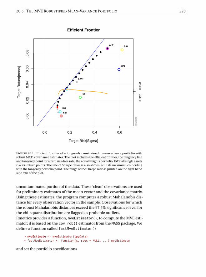
Note that for the Swiss Pension Fund benchmark data set the "covMcdEs-timator" is about 20 time slower than the sample covariance estimator,and the "mcdEstimator" is even slower by a factor of about 300.For the plot we recalculate the frontier on 20 frontier points.

> setNFrontierPoints(covMcdSpec) <- 20> covMcdFrontier <- portfolioFrontier(

data = lppData, spec = covMcdSpec)> tailoredFrontierPlot(

covMcdFrontier,mText = "MCD Robustified MV Portfolio",risk = "Sigma")

The frontier plot is shown in Figure 20.1.To display the weights, risk attributions and covariance risk budgets forthe MCD robustified portfolio in the left-hand column and the same plotsfor the sample covariance MV portfolio in the right-hand column of afigure:

> ## MCD robustified portfolio> par(mfcol = c(3, 2), mar = c(3.5, 4, 4, 3) + 0.1)> col = qualiPalette(30, "Dark2")> weightsPlot(covMcdFrontier, col = col)> text <- "MCD"> mtext(text, side = 3, line = 3, font = 2, cex = 0.9)> weightedReturnsPlot(covMcdFrontier, col = col)> covRiskBudgetsPlot(covMcdFrontier, col = col)> ## Sample covariance MV portfolio> longSpec <- portfolioSpec()> setNFrontierPoints(longSpec) <- 20> longFrontier <- portfolioFrontier(data = lppData, spec = longSpec)> col = qualiPalette(30, "Set1")> weightsPlot(longFrontier, col = col)> text <- "COV"> mtext(text, side = 3, line = 3, font = 2, cex = 0.9)> weightedReturnsPlot(longFrontier, col = col)> covRiskBudgetsPlot(longFrontier, col = col)

The weights, risk attributions and covariance risk budgets are shown inFigure 20.2.

20.3 THE MVE ROBUSTIFIED MEAN-VARIANCE PORTFOLIO

Rousseeuw & Leroy (1987) proposed a very robust alternative to classicalestimates of mean vectors and covariance matrices, the Minimum Vol-ume Ellipsoid, MVE. Samples from a multivariate normal distributionform ellipsoid-shaped ‘clouds’ of data points. The MVE corresponds tothe smallest point cloud containing at least half of the observations, the

20.3. THE MVE ROBUSTIFIED MEAN-VARIANCE PORTFOLIO 223

0.0 0.2 0.4 0.6

0.00

0.02

0.04

0.06

0.08

●

●

●

●

●

●

●

●

●

●

●

●

●

●

●

●

●

●

●

●

Efficient Frontier

Target Risk[Sigma]

Targ

et R

etur

n[m

ean]

Rm

etric

s

●

●

EWP

●

●

●

●

●

●

SBI

SPI

SII

LMI

MPI

ALT

●

0.02

81

0.0

341

Rm

etric

s

FIGURE 20.1: Efficient frontier of a long-only constrained mean-variance portfolio withrobust MCD covariance estimates: The plot includes the efficient frontier, the tangency lineand tangency point for a zero risk-free rate, the equal weights portfolio, EWP, all single assetsrisk vs. return points. The line of Sharpe ratios is also shown, with its maximum coincidingwith the tangency portfolio point. The range of the Sharpe ratio is printed on the right handside axis of the plot.

uncontaminated portion of the data. These ‘clean’ observations are usedfor preliminary estimates of the mean vector and the covariance matrix.Using these estimates, the program computes a robust Mahalanobis dis-tance for every observation vector in the sample. Observations for whichthe robust Mahalanobis distances exceed the 97.5% significance level forthe chi-square distribution are flagged as probable outliers.Rmetrics provides a function, mveEstimator(), to compute the MVE esti-mator; it is based on the cov.rob() estimator from the MASS package. Wedefine a function called fastMveEstimator()

> mveEstimate <- mveEstimator(lppData)> fastMveEstimator <- function(x, spec = NULL, ...) mveEstimate

and set the portfolio specifications


0.0

0.4

0.8 SBI

SPISIILMIMPIALT

0.0

0.4

0.8

0.126 0.15 0.329 0.54

4.07e−05 0.0542 0.0813

Target Risk

Target Return

Wei

ght

Weights

Rm

etric

s

MCD

0.00

0.04

0.08 SBI

SPISIILMIMPIALT

0.00

0.04

0.08

0.126 0.15 0.329 0.54

4.07e−05 0.0542 0.0813

Target Risk

Target Return

Wei

ghte

d R

etur

n

Weighted Returns

Rm

etric

s

0.0

0.4

0.8 SBI

SPISIILMIMPIALT

0.0

0.4

0.8

0.126 0.15 0.329 0.54

4.07e−05 0.0542 0.0813

Target Risk

Target Return

Cov

Ris

k Bu

dget

s

Cov Risk Budgets

Rm

etric

s

0.0

0.4

0.8 SBI

SPISIILMIMPIALT

0.0

0.4

0.8

0.126 0.147 0.322 0.529

4.07e−05 0.0542 0.0813

Target Risk

Target Return

Wei

ght

Weights

Rm

etric

s

COV

0.00

0.04

0.08 SBI

SPISIILMIMPIALT

0.00

0.04

0.08

0.126 0.147 0.322 0.529

4.07e−05 0.0542 0.0813

Target Risk

Target Return

Wei

ghte

d R

etur

n

Weighted Returns

Rm

etric

s

0.0

0.4

0.8 SBI

SPISIILMIMPIALT

0.0

0.4

0.8

0.126 0.147 0.322 0.529

4.07e−05 0.0542 0.0813

Target Risk

Target Return

Cov

Ris

k Bu

dget

s

Cov Risk Budgets

Rm

etric

s

FIGURE 20.2: Weights plot for MCD robustified and COV MV portfolios. Weights along theefficient frontier of a long-only constrained mean-variance portfolio with robust MCD (left)and sample (right) covariance estimates: The graphs from top to bottom show the weights,the weighted returns or in other words the performance attribution, and the covariance riskbudgets, which are a measure for the risk attribution. The upper axis labels the target risk,and the lower labels the target return. The thick vertical line separates the efficient frontierfrom the minimum variance locus. The risk axis thus increases in value to both sides of theseparator line. The legend to the right links the assets names to colour of the bars.

20.3. THE MVE ROBUSTIFIED MEAN-VARIANCE PORTFOLIO 225

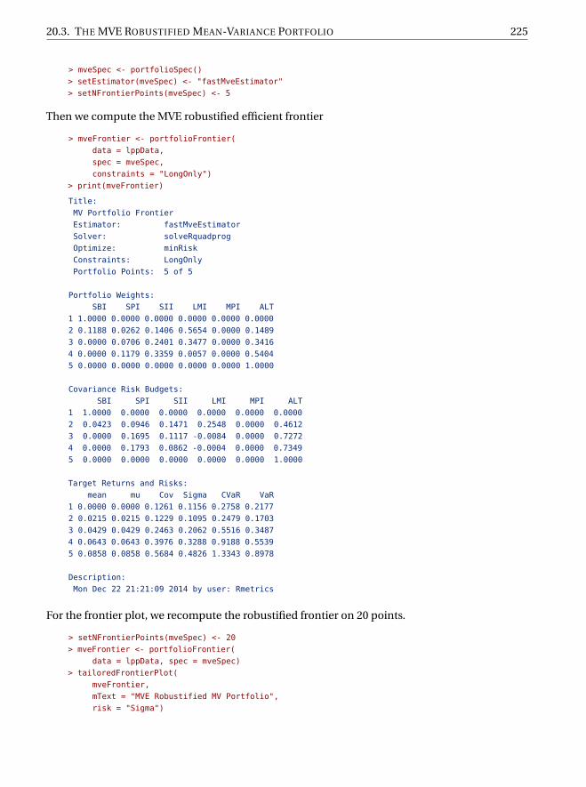
> mveSpec <- portfolioSpec()> setEstimator(mveSpec) <- "fastMveEstimator"> setNFrontierPoints(mveSpec) <- 5

Then we compute the MVE robustified efficient frontier

> mveFrontier <- portfolioFrontier(data = lppData,spec = mveSpec,constraints = "LongOnly")

> print(mveFrontier)

Title:MV Portfolio FrontierEstimator: fastMveEstimatorSolver: solveRquadprogOptimize: minRiskConstraints: LongOnlyPortfolio Points: 5 of 5


1 1.0000 0.0000 0.0000 0.0000 0.0000 0.00002 0.1188 0.0262 0.1406 0.5654 0.0000 0.14893 0.0000 0.0706 0.2401 0.3477 0.0000 0.34164 0.0000 0.1179 0.3359 0.0057 0.0000 0.54045 0.0000 0.0000 0.0000 0.0000 0.0000 1.0000


1 1.0000 0.0000 0.0000 0.0000 0.0000 0.00002 0.0423 0.0946 0.1471 0.2548 0.0000 0.46123 0.0000 0.1695 0.1117 -0.0084 0.0000 0.72724 0.0000 0.1793 0.0862 -0.0004 0.0000 0.73495 0.0000 0.0000 0.0000 0.0000 0.0000 1.0000


1 0.0000 0.0000 0.1261 0.1156 0.2758 0.21772 0.0215 0.0215 0.1229 0.1095 0.2479 0.17033 0.0429 0.0429 0.2463 0.2062 0.5516 0.34874 0.0643 0.0643 0.3976 0.3288 0.9188 0.55395 0.0858 0.0858 0.5684 0.4826 1.3343 0.8978


For the frontier plot, we recompute the robustified frontier on 20 points.

> setNFrontierPoints(mveSpec) <- 20> mveFrontier <- portfolioFrontier(

data = lppData, spec = mveSpec)> tailoredFrontierPlot(

mveFrontier,mText = "MVE Robustified MV Portfolio",risk = "Sigma")


0.0 0.2 0.4 0.6

0.00

0.02

0.04

0.06

0.08

●

●

●

●

●

●

●

●

●

●

●

●

●

●

●

●

●

●

●

●

Efficient Frontier

Target Risk[Sigma]

Targ

et R

etur

n[m

ean]

Rm

etric

s

●

●

EWP

●

●

●

●

●

●

SBI

SPI

SII

LMI

MPI

ALT

●

0.02

71

0.0

324

Rm

etric

s

FIGURE 20.3: Efficient frontier of a long-only constrained mean-variance portfolio withrobust MVE covariance estimates: The plot includes the efficient frontier, the tangency lineand tangency point for a zero risk-free rate, the equal weights portfolio, EWP, all single assetsrisk vs. return points. The line of Sharpe ratios is also shown, with its maximum coincidingwith the tangency portfolio point. The range of the Sharpe ratio is printed on the right handside axis of the plot.

The frontier plot is shown in Figure 20.3.To complete this section, we will show the weights and the performanceand risk attribution plots (left-hand column of Figure 20.4).

> col = divPalette(6, "RdBu")> weightsPlot(mveFrontier, col = col)> boxL()> text <- "MVE Robustified MV Portfolio"> mtext(text, side = 3, line = 3, font = 2, cex = 0.9)> weightedReturnsPlot(mveFrontier, col = col)> boxL()> covRiskBudgetsPlot(mveFrontier, col = col)> boxL()

For the colours we have chosen a diverging red to blue palette. The boxL()

20.4. THE OGK ROBUSTIFIED MEAN-VARIANCE PORTFOLIO 227

0.0

0.4

0.8 SBI

SPISIILMIMPIALT

0.0

0.4

0.8

0.126 0.148 0.325 0.534

4.07e−05 0.0542 0.0813

Target Risk

Target Return

Wei

ght

Weights

Rm

etric

s

MVE0.

000.

040.

08 SBISPISIILMIMPIALT

0.00

0.04

0.08

0.126 0.148 0.325 0.534

4.07e−05 0.0542 0.0813

Target Risk

Target Return

Wei

ghte

d R

etur

n

Weighted Returns

Rm

etric

s

0.0

0.4

0.8 SBI

SPISIILMIMPIALT

0.0

0.4

0.8

0.126 0.148 0.325 0.534

4.07e−05 0.0542 0.0813

Target Risk

Target Return

Cov

Ris

k Bu

dget

s

Cov Risk Budgets

Rm

etric

s

0.0

0.4

0.8 SBI

SPISIILMIMPIALT

0.0

0.4

0.8

0.126 0.15 0.329 0.54

4.07e−05 0.0542 0.0813

Target Risk

Target Return

Wei

ght

Weights

Rm

etric

s

MCD

0.00

0.04

0.08 SBI

SPISIILMIMPIALT

0.00

0.04

0.08

0.126 0.15 0.329 0.54

4.07e−05 0.0542 0.0813

Target Risk

Target Return

Wei

ghte

d R

etur

n

Weighted Returns

Rm

etric

s

0.0

0.4

0.8 SBI

SPISIILMIMPIALT

0.0

0.4

0.8

0.126 0.15 0.329 0.54

4.07e−05 0.0542 0.0813

Target Risk

Target Return

Cov

Ris

k Bu

dget

s

Cov Risk Budgets

Rm

etric

s

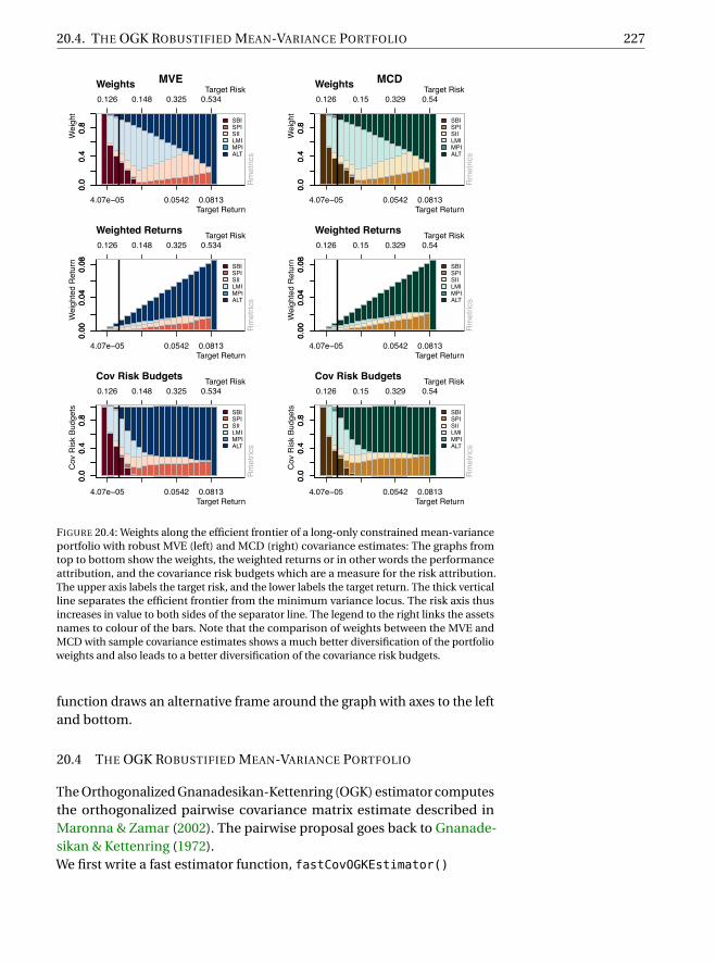
FIGURE 20.4: Weights along the efficient frontier of a long-only constrained mean-varianceportfolio with robust MVE (left) and MCD (right) covariance estimates: The graphs fromtop to bottom show the weights, the weighted returns or in other words the performanceattribution, and the covariance risk budgets which are a measure for the risk attribution.The upper axis labels the target risk, and the lower labels the target return. The thick verticalline separates the efficient frontier from the minimum variance locus. The risk axis thusincreases in value to both sides of the separator line. The legend to the right links the assetsnames to colour of the bars. Note that the comparison of weights between the MVE andMCD with sample covariance estimates shows a much better diversification of the portfolioweights and also leads to a better diversification of the covariance risk budgets.

function draws an alternative frame around the graph with axes to the leftand bottom.

20.4 THE OGK ROBUSTIFIED MEAN-VARIANCE PORTFOLIO

The Orthogonalized Gnanadesikan-Kettenring (OGK) estimator computesthe orthogonalized pairwise covariance matrix estimate described inMaronna & Zamar (2002). The pairwise proposal goes back to Gnanade-sikan & Kettenring (1972).We first write a fast estimator function, fastCovOGKEstimator()


> covOGKEstimate <- covOGKEstimator(lppData)> fastCovOGKEstimator <- function(x, spec = NULL, ...) covOGKEstimate

then we set the portfolio specification

> covOGKSpec <- portfolioSpec()> setEstimator(covOGKSpec) <- "fastCovOGKEstimator"> setNFrontierPoints(covOGKSpec) <- 5

and finally we compute the OGK robustified frontier

> covOGKFrontier <- portfolioFrontier(data = lppData, spec = covOGKSpec)

> print(covOGKFrontier)

Title:MV Portfolio FrontierEstimator: fastCovOGKEstimatorSolver: solveRquadprogOptimize: minRiskConstraints: LongOnlyPortfolio Points: 5 of 5


1 1.0000 0.0000 0.0000 0.0000 0.0000 0.00002 0.0990 0.0171 0.1593 0.5723 0.0000 0.15223 0.0000 0.0650 0.2661 0.3277 0.0000 0.34114 0.0000 0.1179 0.3433 0.0000 0.0000 0.53885 0.0000 0.0000 0.0000 0.0000 0.0000 1.0000


1 1.0000 0.0000 0.0000 0.0000 0.0000 0.00002 0.0347 0.0583 0.1827 0.2605 0.0000 0.46393 0.0000 0.1540 0.1329 -0.0089 0.0000 0.72214 0.0000 0.1790 0.0895 0.0000 0.0000 0.73155 0.0000 0.0000 0.0000 0.0000 0.0000 1.0000


1 0.0000 0.0000 0.1261 0.1270 0.2758 0.21772 0.0215 0.0215 0.1223 0.1197 0.2419 0.17413 0.0429 0.0429 0.2460 0.2222 0.5450 0.34184 0.0643 0.0643 0.3976 0.3532 0.9175 0.55235 0.0858 0.0858 0.5684 0.5236 1.3343 0.8978


> setNFrontierPoints(covOGKSpec) <- 20> covOGKFrontier <- portfolioFrontier(

data = lppData, spec = covOGKSpec)> tailoredFrontierPlot(

covOGKFrontier,mText = "OGK Robustified MV Portfolio",

20.4. THE OGK ROBUSTIFIED MEAN-VARIANCE PORTFOLIO 229

0.0 0.2 0.4 0.6

0.00

0.02

0.04

0.06

0.08

●

●

●

●

●

●

●

●

●

●

●

●

●

●

●

●

●

●

●

●

Efficient Frontier

Target Risk[Sigma]

Targ

et R

etur

n[m

ean]

Rm

etric

s

●

●

EWP

●

●

●

●

●

●

SBI

SPI

SII

LMI

MPI

ALT

●

0.02

78

0.0

333

Rm

etric

s

FIGURE 20.5: Efficient frontier of a long-only constrained mean-variance portfolio withrobust OGK covariance estimates: The plot includes the efficient frontier, the tangency lineand tangency point for a zero risk-free rate, the equal weights portfolio, EWP, all single assetsrisk vs. return points. The line of Sharpe ratios is also shown, with its maximum coincidingwith the tangency portfolio point. The range of the Sharpe ratio is printed on the right handside axis of the plot.

risk = "Sigma")

The frontier plot is shown in Figure 20.5.The weights, and the performance and risk attributions are shown in theleft-hand column of Figure 20.6.

> col = divPalette(6, "RdYlGn")> weightsPlot(covOGKFrontier, col = col)> text <- "OGK Robustified MV Portfolio"> mtext(text, side = 3, line = 3, font = 2, cex = 0.9)> weightedReturnsPlot(covOGKFrontier, col = col)> covRiskBudgetsPlot(covOGKFrontier, col = col)


0.0

0.4

0.8 SBI

SPISIILMIMPIALT

0.0

0.4

0.8

0.126 0.148 0.325 0.535

4.07e−05 0.0542 0.0813

Target Risk

Target Return

Wei

ght

Weights

Rm

etric

s

OGK

0.00

0.04

0.08 SBI

SPISIILMIMPIALT

0.00

0.04

0.08

0.126 0.148 0.325 0.535

4.07e−05 0.0542 0.0813

Target Risk

Target Return

Wei

ghte

d R

etur

n

Weighted Returns

Rm

etric

s

0.0

0.4

0.8 SBI

SPISIILMIMPIALT

0.0

0.4

0.8

0.126 0.148 0.325 0.535

4.07e−05 0.0542 0.0813

Target Risk

Target Return

Cov

Ris

k Bu

dget

s

Cov Risk Budgets

Rm

etric

s

0.0

0.4

0.8 SBI

SPISIILMIMPIALT

0.0

0.4

0.8

0.126 0.15 0.329 0.54

4.07e−05 0.0542 0.0813

Target Risk

Target Return

Wei

ght

Weights

Rm

etric

s

MCD

0.00

0.04

0.08 SBI

SPISIILMIMPIALT

0.00

0.04

0.08

0.126 0.15 0.329 0.54

4.07e−05 0.0542 0.0813

Target Risk

Target Return

Wei

ghte

d R

etur

n

Weighted Returns

Rm

etric

s

0.0

0.4

0.8 SBI

SPISIILMIMPIALT

0.0

0.4

0.8

0.126 0.15 0.329 0.54

4.07e−05 0.0542 0.0813

Target Risk

Target Return

Cov

Ris

k Bu

dget

s

Cov Risk BudgetsR

met

rics

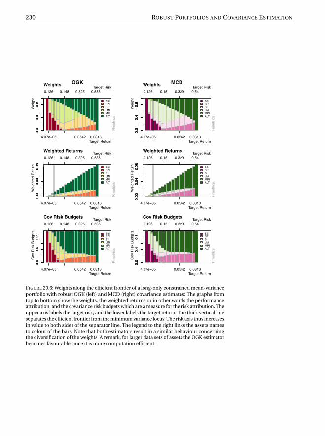
FIGURE 20.6: Weights along the efficient frontier of a long-only constrained mean-varianceportfolio with robust OGK (left) and MCD (right) covariance estimates: The graphs fromtop to bottom show the weights, the weighted returns or in other words the performanceattribution, and the covariance risk budgets which are a measure for the risk attribution. Theupper axis labels the target risk, and the lower labels the target return. The thick vertical lineseparates the efficient frontier from the minimum variance locus. The risk axis thus increasesin value to both sides of the separator line. The legend to the right links the assets namesto colour of the bars. Note that both estimators result in a similar behaviour concerningthe diversification of the weights. A remark, for larger data sets of assets the OGK estimatorbecomes favourable since it is more computation efficient.

20.5. THE SHRINKED MEAN-VARIANCE PORTFOLIO 231

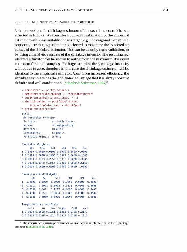
20.5 THE SHRINKED MEAN-VARIANCE PORTFOLIO

A simple version of a shrinkage estimator of the covariance matrix is con-structed as follows. We consider a convex combination of the empiricalestimator with some suitable chosen target, e.g., the diagonal matrix. Sub-sequently, the mixing parameter is selected to maximize the expected ac-curacy of the shrinked estimator. This can be done by cross-validation, orby using an analytic estimate of the shrinkage intensity. The resulting reg-ularized estimator can be shown to outperform the maximum likelihoodestimator for small samples. For large samples, the shrinkage intensitywill reduce to zero, therefore in this case the shrinkage estimator will beidentical to the empirical estimator. Apart from increased efficiency, theshrinkage estimate has the additional advantage that it is always positivedefinite and well conditioned, (Schäfer & Strimmer, 2005)2.

> shrinkSpec <- portfolioSpec()> setEstimator(shrinkSpec) <- "shrinkEstimator"> setNFrontierPoints(shrinkSpec) <- 5> shrinkFrontier <- portfolioFrontier(

data = lppData, spec = shrinkSpec)> print(shrinkFrontier)

Title:MV Portfolio FrontierEstimator: shrinkEstimatorSolver: solveRquadprogOptimize: minRiskConstraints: LongOnlyPortfolio Points: 5 of 5


1 1.0000 0.0000 0.0000 0.0000 0.0000 0.00002 0.0328 0.0020 0.1498 0.6507 0.0000 0.16473 0.0000 0.0193 0.2550 0.3372 0.0000 0.38854 0.0000 0.0378 0.3454 0.0000 0.0000 0.61685 0.0000 0.0000 0.0000 0.0000 0.0000 1.0000


1 1.0000 0.0000 0.0000 0.0000 0.0000 0.00002 0.0111 0.0062 0.1629 0.3231 0.0000 0.49683 0.0000 0.0422 0.1227 -0.0096 0.0000 0.84474 0.0000 0.0527 0.0893 0.0000 0.0000 0.85805 0.0000 0.0000 0.0000 0.0000 0.0000 1.0000


1 0.0000 0.0000 0.1261 0.1261 0.2758 0.21772 0.0215 0.0215 0.1214 0.1217 0.2368 0.1810

2 The covariance shrinkage estimator we use here is implemented in the R packagecorpcor (Schaefer et al., 2008).


0.0 0.2 0.4 0.6 0.8

0.00

0.02

0.04

0.06

0.08

●

●

●

●

●

●

●

●

●

●

●

●

●

●

●

●

●

●

●

●

Efficient Frontier

Target Risk[Sigma]

Targ

et R

etur

n[m

ean]

Rm

etric

s

●

●

EWP

●

●

●

●

●

●

SBI

SPI

SII

LMI

MPI

ALT

●

0.02

34

0.0

285

Rm

etric

s

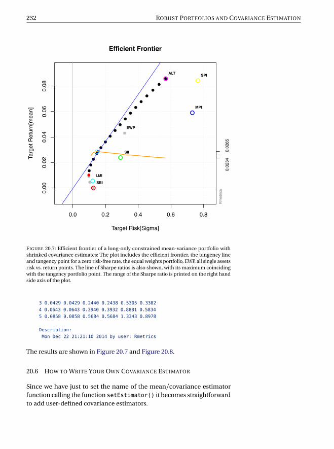
FIGURE 20.7: Efficient frontier of a long-only constrained mean-variance portfolio withshrinked covariance estimates: The plot includes the efficient frontier, the tangency lineand tangency point for a zero risk-free rate, the equal weights portfolio, EWP, all single assetsrisk vs. return points. The line of Sharpe ratios is also shown, with its maximum coincidingwith the tangency portfolio point. The range of the Sharpe ratio is printed on the right handside axis of the plot.

3 0.0429 0.0429 0.2440 0.2438 0.5305 0.33824 0.0643 0.0643 0.3940 0.3932 0.8881 0.58345 0.0858 0.0858 0.5684 0.5684 1.3343 0.8978


The results are shown in Figure 20.7 and Figure 20.8.

20.6 HOW TO WRITE YOUR OWN COVARIANCE ESTIMATOR

Since we have just to set the name of the mean/covariance estimatorfunction calling the function setEstimator() it becomes straightforwardto add user-defined covariance estimators.

20.6. HOW TO WRITE YOUR OWN COVARIANCE ESTIMATOR 233

0.0

0.4

0.8 SBI

SPISIILMIMPIALT

0.0

0.4

0.8

0.126 0.147 0.322 0.529

4.07e−05 0.0271 0.0542 0.0813

Target Risk

Target Return

Wei

ght

Weights

Rm

etric

s

Shrinked MV Portfolio

0.00

0.04

0.08 SBI

SPISIILMIMPIALT

0.00

0.04

0.08

0.126 0.147 0.322 0.529

4.07e−05 0.0271 0.0542 0.0813

Target Risk

Target Return

Wei

ghte

d R

etur

n

Weighted Returns

Rm

etric

s

0.0

0.4

0.8 SBI

SPISIILMIMPIALT

0.0

0.4

0.8

0.126 0.147 0.322 0.529

4.07e−05 0.0271 0.0542 0.0813

Target Risk

Target Return

Cov

Ris

k Bu

dget

s

Cov Risk Budgets

Rm

etric

s

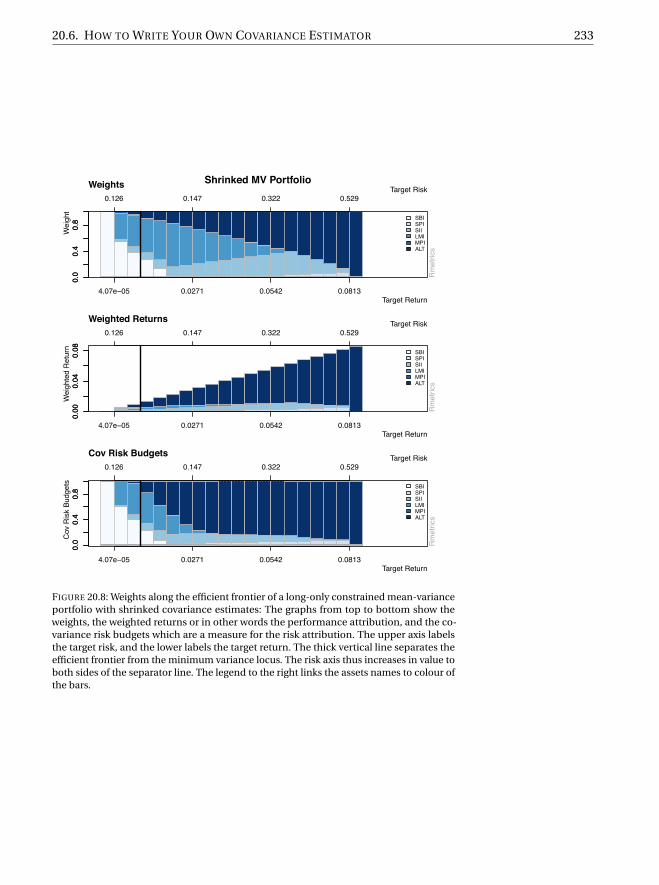
FIGURE 20.8: Weights along the efficient frontier of a long-only constrained mean-varianceportfolio with shrinked covariance estimates: The graphs from top to bottom show theweights, the weighted returns or in other words the performance attribution, and the co-variance risk budgets which are a measure for the risk attribution. The upper axis labelsthe target risk, and the lower labels the target return. The thick vertical line separates theefficient frontier from the minimum variance locus. The risk axis thus increases in value toboth sides of the separator line. The legend to the right links the assets names to colour ofthe bars.


Let us show an example. InR’s recommended package MASS there is a func-tion (cov.trob()) which estimates a covariance matrix assuming the datacome from a multivariate Student’s t distribution. This approach providessome degree of robustness to outliers without giving a high breakdownpoint3.

> covtEstimator <- function (x, spec = NULL, ...) {x.mat = as.matrix(x)list(mu = colMeans(x.mat), Sigma = MASS::cov.trob(x.mat)$cov) }

> covtSpec <- portfolioSpec()> setEstimator(covtSpec) <- "covtEstimator"> setNFrontierPoints(covtSpec) <- 5> covtFrontier <- portfolioFrontier(

data = lppData, spec = covtSpec)> print(covtFrontier)

Title:MV Portfolio FrontierEstimator: covtEstimatorSolver: solveRquadprogOptimize: minRiskConstraints: LongOnlyPortfolio Points: 5 of 5


1 1.0000 0.0000 0.0000 0.0000 0.0000 0.00002 0.0749 0.0156 0.1490 0.6061 0.0000 0.15443 0.0000 0.0517 0.2479 0.3420 0.0000 0.35834 0.0000 0.0896 0.3441 0.0000 0.0000 0.56635 0.0000 0.0000 0.0000 0.0000 0.0000 1.0000


1 1.0000 0.0000 0.0000 0.0000 0.0000 0.00002 0.0260 0.0527 0.1627 0.2873 0.0000 0.47143 0.0000 0.1205 0.1179 -0.0089 0.0000 0.77064 0.0000 0.1326 0.0897 0.0000 0.0000 0.77775 0.0000 0.0000 0.0000 0.0000 0.0000 1.0000


1 0.0000 0.0000 0.1261 0.1109 0.2758 0.21772 0.0215 0.0215 0.1220 0.1043 0.2420 0.17413 0.0429 0.0429 0.2451 0.2006 0.5424 0.34324 0.0643 0.0643 0.3958 0.3217 0.9066 0.56455 0.0858 0.0858 0.5684 0.4697 1.3343 0.8978


3Intuitively, the breakdown point of an estimator is the proportion of incorrect observa-tions an estimator can handle before giving an arbitrarily unreasonable result

20.6. HOW TO WRITE YOUR OWN COVARIANCE ESTIMATOR 235

0.0 0.2 0.4 0.6

0.00

0.02

0.04

0.06

0.08

●

●

●

●

●

●

●

●

●

●

●

●

●

●

●

●

●

●

●

●

Efficient Frontier

Target Risk[Sigma]

Targ

et R

etur

n[m

ean]

Rm

etric

s

●

●

EWP

●

●

●

●

●

●

SBI

SPI

SII

LMI

MPI

ALT

●

0.02

56

0.0

309

Rm

etric

s

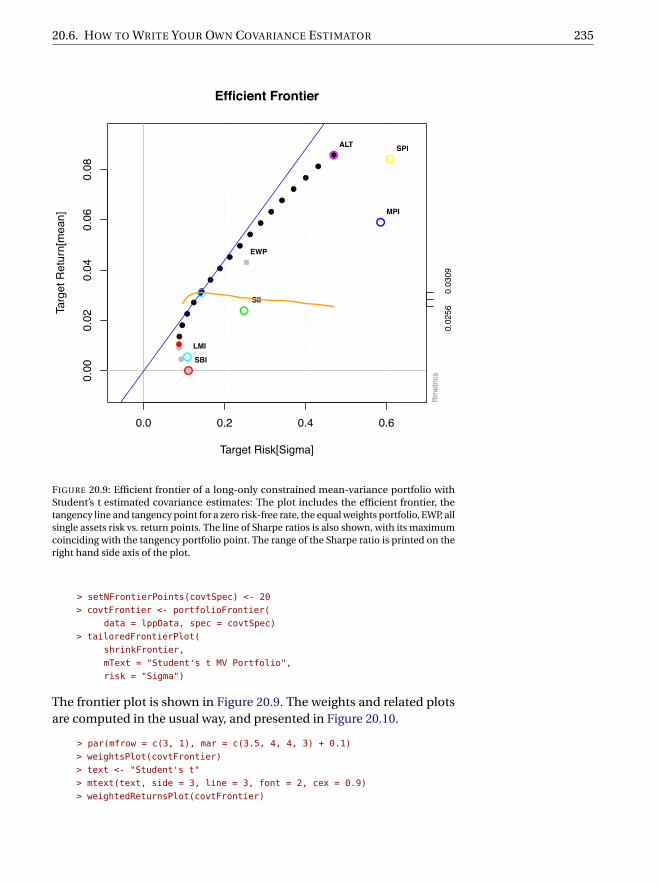
FIGURE 20.9: Efficient frontier of a long-only constrained mean-variance portfolio withStudent’s t estimated covariance estimates: The plot includes the efficient frontier, thetangency line and tangency point for a zero risk-free rate, the equal weights portfolio, EWP, allsingle assets risk vs. return points. The line of Sharpe ratios is also shown, with its maximumcoinciding with the tangency portfolio point. The range of the Sharpe ratio is printed on theright hand side axis of the plot.

> setNFrontierPoints(covtSpec) <- 20> covtFrontier <- portfolioFrontier(

data = lppData, spec = covtSpec)> tailoredFrontierPlot(

shrinkFrontier,mText = "Student's t MV Portfolio",risk = "Sigma")

The frontier plot is shown in Figure 20.9. The weights and related plotsare computed in the usual way, and presented in Figure 20.10.

> par(mfrow = c(3, 1), mar = c(3.5, 4, 4, 3) + 0.1)> weightsPlot(covtFrontier)> text <- "Student's t"> mtext(text, side = 3, line = 3, font = 2, cex = 0.9)> weightedReturnsPlot(covtFrontier)


0.0

0.4

0.8 SBI

SPISIILMIMPIALT

0.0

0.4

0.8

0.126 0.148 0.323 0.532

4.07e−05 0.0271 0.0542 0.0813

Target Risk

Target Return

Wei

ght

Weights

Rm

etric

s

Student's t0.

000.

040.

08 SBISPISIILMIMPIALT

0.00

0.04

0.08

0.126 0.148 0.323 0.532

4.07e−05 0.0271 0.0542 0.0813

Target Risk

Target Return

Wei

ghte

d R

etur

n

Weighted Returns

Rm

etric

s

0.0

0.4

0.8 SBI

SPISIILMIMPIALT

0.0

0.4

0.8

0.126 0.148 0.323 0.532

4.07e−05 0.0271 0.0542 0.0813

Target Risk

Target Return

Cov

Ris

k Bu

dget

s

Cov Risk Budgets

Rm

etric

s

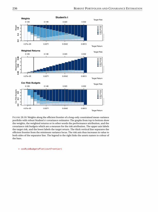
FIGURE 20.10: Weights along the efficient frontier of a long-only constrained mean-varianceportfolio with robust Student’s t covariance estimates: The graphs from top to bottom showthe weights, the weighted returns or in other words the performance attribution, and thecovariance risk budgets which are a measure for the risk attribution. The upper axis labelsthe target risk, and the lower labels the target return. The thick vertical line separates theefficient frontier from the minimum variance locus. The risk axis thus increases in value toboth sides of the separator line. The legend to the right links the assets names to colour ofthe bars.

> covRiskBudgetsPlot(covtFrontier)

rmetrics user guides · a.10 rmetrics package: fportfoliobacktest. . . . . . . . . . . . . . . ....

Documents