rms.technictrang.ac.thrms.technictrang.ac.th/files/3920600658739_13100311115933.pdf · chapter9 273...
TRANSCRIPT

9C H A P T E R
273
Strengthof MaterialsJames R. Hutchinson
OUTLINE
AXIALLY LOADED MEMBERS 274Modulus of Elasticity � Poisson’s Ratio � Thermal Deformations � Variable Load
THIN-WALLED CYLINDER 280
GENERAL STATE OF STRESS 282
PLANE STRESS 283Mohr’s Circle—Stress
STRAIN 286Plane Strain
HOOKE’S LAW 288
TORSION 289Circular Shafts � Hollow, Thin-Walled Shafts
BEAMS 292Shear and Moment Diagrams � Stresses in Beams � Shear Stress � Deflection of Beams � Fourth-Order BeamEquation � Superposition
COMBINED STRESS 307
COLUMNS 309
SELECTED SYMBOLS AND ABBREVIATIONS 311
PROBLEMS 312
SOLUTIONS 319
Mechanics of materials deals with the determination of the internal forces(stresses) and the deformation of solids such as metals, wood, concrete, plasticsand composites. In mechanics of materials there are three main considerations inthe solution of problems:
FundEng_Index.book Page 273 Wednesday, November 28, 2007 4:42 PM
274 Chapter 9 Strength of Materials
1. Equilibrium
2. Force-deformation relations
3. Compatibility
Equilibrium refers to the equilibrium of forces. The laws of statics must holdfor the body and all parts of the body. Force-deformation relations refer to therelation of the applied forces to the deformation of the body. If certain forces areapplied, then certain deformations will result. Compatibility refers to the compat-ibility of deformation. Upon loading, the parts of a body or structure must notcome apart. These three principles will be emphasized throughout.
AXIALLY LOADED MEMBERS
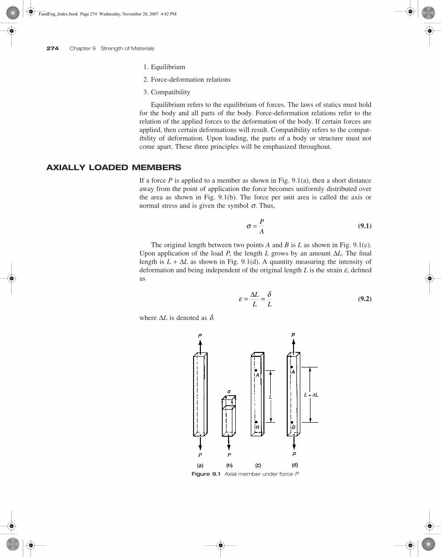
If a force P is applied to a member as shown in Fig. 9.1(a), then a short distanceaway from the point of application the force becomes uniformly distributed overthe area as shown in Fig. 9.1(b). The force per unit area is called the axis ornormal stress and is given the symbol s. Thus,
(9.1)
The original length between two points A and B is L as shown in Fig. 9.1(c).Upon application of the load P, the length L grows by an amount ∆L. The finallength is L + ∆L as shown in Fig. 9.1(d). A quantity measuring the intensity ofdeformation and being independent of the original length L is the strain e, definedas
(9.2)
where ∆L is denoted as d.
Figure 9.1 Axial member under force P
σ = PA
ε δ= =∆LL L
FundEng_Index.book Page 274 Wednesday, November 28, 2007 4:42 PM
Axially Loaded Members 275
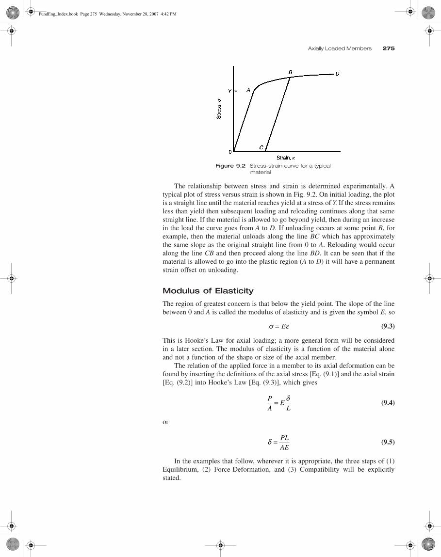
The relationship between stress and strain is determined experimentally. Atypical plot of stress versus strain is shown in Fig. 9.2. On initial loading, the plotis a straight line until the material reaches yield at a stress of Y. If the stress remainsless than yield then subsequent loading and reloading continues along that samestraight line. If the material is allowed to go beyond yield, then during an increasein the load the curve goes from A to D. If unloading occurs at some point B, forexample, then the material unloads along the line BC which has approximatelythe same slope as the original straight line from 0 to A. Reloading would occuralong the line CB and then proceed along the line BD. It can be seen that if thematerial is allowed to go into the plastic region (A to D) it will have a permanentstrain offset on unloading.
Modulus of Elasticity
The region of greatest concern is that below the yield point. The slope of the linebetween 0 and A is called the modulus of elasticity and is given the symbol E, so
s = Ee (9.3)
This is Hooke’s Law for axial loading; a more general form will be consideredin a later section. The modulus of elasticity is a function of the material aloneand not a function of the shape or size of the axial member.
The relation of the applied force in a member to its axial deformation can befound by inserting the definitions of the axial stress [Eq. (9.1)] and the axial strain[Eq. (9.2)] into Hooke’s Law [Eq. (9.3)], which gives
(9.4)
or
(9.5)
In the examples that follow, wherever it is appropriate, the three steps of (1)Equilibrium, (2) Force-Deformation, and (3) Compatibility will be explicitlystated.
Figure 9.2 Stress-strain curve for a typical material
PA
EL
= δ
δ = PLAE
FundEng_Index.book Page 275 Wednesday, November 28, 2007 4:42 PM
276 Chapter 9 Strength of Materials
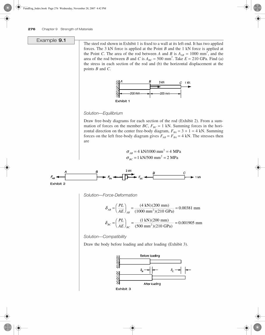
Example 9.1The steel rod shown in Exhibit 1 is fixed to a wall at its left end. It has two appliedforces. The 3 kN force is applied at the Point B and the 1 kN force is applied atthe Point C. The area of the rod between A and B is AAB = 1000 mm2, and thearea of the rod between B and C is ABC = 500 mm2. Take E = 210 GPa. Find (a)the stress in each section of the rod and (b) the horizontal displacement at thepoints B and C.
Solution—Equilibrium
Draw free-body diagrams for each section of the rod (Exhibit 2). From a sum-mation of forces on the member BC, FBC = 1 kN. Summing forces in the hori-zontal direction on the center free-body diagram, FBA = 3 + 1 = 4 kN. Summingforces on the left free-body diagram gives FAB = FBA = 4 kN. The stresses thenare
Solution—Force-Deformation
Solution—Compatibility
Draw the body before loading and after loading (Exhibit 3).
Exhibit 1
σσ
AB
BC
= == =
4 4
1
kN/1000 mm MPa
kN/500 mm 2 MPa
2
2
Exhibit 2
Exhibit 3
δ
δ
ABAB
BCBC
PL
AE
PL
AE
=
= =
=
= =
( )( ).
( )( )( )( )
.
4 200210
0 00381
1 200210
0 001905
kN mm(1000 mm )( GPa)
mm
kN mm500 mm GPa
mm
2
2
FundEng_Index.book Page 276 Wednesday, November 28, 2007 4:42 PM

Axially Loaded Members 277
It is then obvious that
In this first example the problem was statically determinate, and the threesteps of Equilibrium, Force-Deformation, and Compatibility were independentsteps. The steps are not independent when the problem is statically indeterminate,as the next example will show.
Example 9.2Consider the same steel rod as in Example 9.1 except that now the right end isfixed to a wall as well as the left (Exhibit 4). It is assumed that the rod is builtinto the walls before the load is applied. Find (a) the stress in each section of therod, and (b) the horizontal displacement at the point B.
Solution—Equilibrium
Draw free-body diagrams for each section of the rod (Exhibit 5). Summing forcesin the horizontal direction on the center free-body diagram
It can be seen that the forces cannot be determined by statics alone so that theother steps must be completed before the stresses in the rods can be determined.
Solution—Force-Deformation
The equilibrium, force-deformation, and compatibility equations can now besolved as follows (see Exhibit 6). The force-deformation relations are put into thecompatibility equations:
δ δB AB= = 0 00381. mm
δ δ δC AB BC= + = + =0 00381 0 001905 0 00571. . . mm
Exhibit 4
− + + =F FAB BC 3 0
Exhibit 5
δ ABAB
AB
AB
PL
AE
F L
A E=
=
δ BCBC
BC
BC
PL
AE
F L
A=
=
F L
A E
F L
A EAB
BC
BC
BC2= −
FundEng_Index.book Page 277 Wednesday, November 28, 2007 4:42 PM

278 Chapter 9 Strength of Materials
Then, FAB = −2FBC. Insert this relationship into the equilibrium equation
The stresses are
The displacement at B is
Poisson’s Ratio
The axial member shown in Fig. 9.1 also has a strain in the lateral direction. Ifthe rod is in tension, then stretching takes place in the longitudinal directionwhile contraction takes place in the lateral direction. The ratio of the magnitudeof the lateral strain to the magnitude of the longitudinal strain is called Poisson’sratio n.
(9.6)
Poisson’s ratio is a dimensionless material property that never exceeds 0.5.Typical values for steel, aluminum, and copper are 0.30, 0.33, and 0.34, respectively.
Example 9.3A circular aluminum rod 10 mm in diameter is loaded with an axial force of2 kN. What is the decrease in diameter of the rod? Take E = 70 GN/m2 andv = 0.33.
Solution
The stress isThe longitudinal strain isThe lateral strain isThe decrease in diameter is then
Exhibit 6
− + + = = + + = − =F F F F F FAB BC BC BC BC AB3 0 2 3 1 2; kN and kN
σσ
AB
BC
= == − = −
2 2
1 2
kN/1000 mm MPa (tension)
kN/500 mm MPa (compression)
2
2
δ δA AB ABF L AE= = = =/( ) ( )( )/[( )(2 200 1000 210 kN mm mm GPa)] 0.001905mm2
ν = − Lateral strainLongitudinal strain
σ π= = = =P A/ kN/ 5 mm GN/m MN/m2 2 2 22 0 0255 25 5( ) . .ε σ1 70 0 000364on
2/E (25.5 MN/m ) GN/m= = =/( ) .ε ε1at on = − = − = −v 1 0 33 0 000364 0 000120. ( . ) .
− = − − =D mm 0.000120) mm1atε ( )( .10 0 00120
FundEng_Index.book Page 278 Wednesday, November 28, 2007 4:42 PM

Axially Loaded Members 279
Thermal Deformations
When a material is heated, expansion forces are created. If it is free to expand,the thermal strain is
(9.7)
where a is the linear coefficient of thermal expansion, t is the final temperatureand t0 is the initial temperature. Since strain is dimensionless, the units of a are°F−1 or °C−1 (sometimes the units are given as in/in/°F or m/m/°C which amountsto the same thing). The total strain is equal to the strain from the applied loadsplus the thermal strain. For problems where the load is purely axial, this becomes
(9.8)
The deformation d is found by multiplying the strain by the length L
(9.9)
Example 9.4 A steel bolt is put through an aluminum tube as shown in Exhibit 7. The nut ismade just tight. The temperature of the entire assembly is then raised by 60°C.Because aluminum expands more than steel, the bolt will be put in tension andthe tube in compression. Find the force in the bolt and the tube. For the steel bolt,take E = 210 GPa, a = 12 × 10−6 °C−1 and A = 32 mm2. For the aluminum tube,take E = 69 GPa, a = 23 × 10−6 °C−1 and A = 64 mm2.
Solution—Equilibrium
Draw free-body diagrams (Exhibit 8). From equilibrium of the bolt it can be seen that PB = PT .
Solution—Force-Deformation
Note that both members have the same length and the same force, P.
The minus sign in the second expression occurs because the tube is in compression.
ε αt t t= −( )0
εT
ε σ αT Et t= + −( )0
δ α= + −PL
AEL t t( )0
Exhibit 8
Exhibit 7
δ αBB B
B
PL
A EL t t= + −( )0
δ αTT T
T
PL
A EL t t= − + −( )0
FundEng_Index.book Page 279 Wednesday, November 28, 2007 4:42 PM

280 Chapter 9 Strength of Materials
Solution—Compatibility
The tube and bolt must both expand the same amount, therefore,
Solving for P gives P = 1.759 kN.
Variable Load
In certain cases the load in the member will not be constant but will be a continuousfunction of the length. These cases occur when there is a distributed load on themember. Such distributed loads most commonly occur when the member is sub-jected to gravitation, acceleration or magnetic fields. In such cases, Eq. (9.5) holdsonly over an infinitesimally small length L = dx. Eq. (9.5) then becomes
(9.10)
or equivalently
(9.11)
Example 9.5 An aluminum rod is hanging from one end. The rod is 1 m long and has a squarecross-section 20 mm by 20 mm. Find the total extension of the rod resulting fromits own weight. Take E = 70 GPa and the unit weight g = 27 kN/m3.
Solution—Equilibrium
Draw a free-body diagram (Exhibit 9). The weight of the section shown in Exhibit 9 is
which clearly yields P as a function of x, and Eq. (9.11) gives
THIN-WALLED CYLINDER
Consider the thin-walled circular cylinder subjected to a uniform internal pressureq as shown in Fig. 9.3. A section of length a, is cut out of the vessel in (a). Thecut-out portion is shown in (b). The pressure q can be considered as acting across
δ δB T=
δ δB T
P
P
= = ××
+ ×°
× × °
− ××
+ ×°
× × °
−
−
( )
( )
100210
12 101
100
6923 10
1100
6
6
mm32 mm GPa C
mm 60 C
=100 mm
64 mm GPa C mm 60 C
2
2
dP x
AEdxδ = ( )
δ = ∫ P xAE
dxL ( )
0
Exihibit 9
W V Ax P= = =γ γ
δ γ γ γ µ= = = =
=∫ ∫AxAE
dxE
xdxLE
L L
0 0
22
2
27 1
2 700 1929
3
kN
m
GN
m
m) m
2
(.
FundEng_Index.book Page 280 Wednesday, November 28, 2007 4:42 PM

Thin-Walled Cylinder 281
the diameter as shown. The tangential stress st is assumed constant through thethickness. Summing forces in the vertical direction gives
(9.12)
(9.13)
where D is the inner diameter of the cylinder and t is the wall thickness. The axialstress is also assumed to be uniform over the wall thickness. The axial stresscan be found by making a cut through the cylinder as shown in (c). Consider thehorizontal equilibrium for the free-body diagram shown in (d). The pressure qacts over the area and the stress sa acts over the area which gives
(9.14)
so
(9.15)
Example 9.6Consider a cylindrical pressure vessel with a wall thickness of 25 mm, an internalpressure of 1.4 MPa, and an outer diameter of 1.2 m. Find the axial and tangentialstresses.
Solution
Figure 9.3
qDa tat− =2 0σ
σ t
qDt
=2
σa
πr2 πDt
σ π πa Dt qD=
2
2
σ a
qDt
=4
q D t
qDt
qDt
t
a
= = − = =
= = ××
=
= = ××
=
1 4 1200 50 1150
21 4
32 2
41 4
16 1
.
..
..
MPa; mm; 25 mm
MPa 1150 mm2 25 mm
MPa
MPa 1150 mm4 25 mm
MPa
σ
σ
FundEng_Index.book Page 281 Wednesday, November 28, 2007 4:42 PM

282 Chapter 9 Strength of Materials
GENERAL STATE OF STRESS
Stress is defined as force per unit area acting on a certain area. Consider a bodythat is cut so that its area has an outward normal in the x direction as shown inFig. 9.4. The force ΔF that is acting over the area ΔAx can be split into itscomponents ΔFx, ΔFy, and ΔFz. The stress components acting on this face are thendefined as
(9.16)
(9.17)
(9.18)
The stress component is the normal stress. It acts normal to the x face in the xdirection. The stress component is a shear stress. It acts parallel to the x facein the y direction. The stress component is also a shear stress and acts parallelto the x face in the z direction. For shear stress, the first subscript indicates theface on which it acts, and the second subscript indicates the direction in which itacts. For normal stress, the single subscript indicates both face and direction. Inthe general state of stress, there are normal and shear stresses on all faces of anelement as shown in Fig. 9.5.
Figure 9.4 Stress on a face
Figure 9.5 Stress at a point (shown in positive directions)
σ x A
x
xx
F
A=
→lim
Δ
ΔΔ0
τ xy A
y
xx
F
A=
→lim
Δ
ΔΔ0
τ xz A
z
xx
F
A=
→lim
Δ
ΔΔ0
σ x
τ xy
τ xz
Chapter 09.fm Page 282 Tuesday, March 4, 2008 12:43 PM
Plane Stress 283
From equilibrium of moments around axes parallel to x, y, and z and passingthrough the center of the element in Fig. 9.5, it can be shown that the followingrelations hold
(9.19)
Thus, at any point in a body the state of stress is given by six components: The usual sign convention is to take the components
shown in Fig. 9.5 as positive. One way of saying this is that normal stresses arepositive in tension. Shear stresses are positive on a positive face in the positivedirection. A positive face is defined as a face with a positive outward normal.
PLANE STRESS
In elementary mechanics of materials, we usually deal with a state of plane stressin which only the stresses in the x-y plane are non-zero. The stress components
are taken as zero.
Mohr’s Circle—Stress
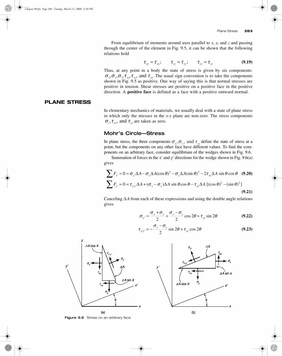
In plane stress, the three components define the state of stress at apoint, but the components on any other face have different values. To find the com-ponents on an arbitrary face, consider equilibrium of the wedges shown in Fig. 9.6.
Summation of forces in the x′ and y′ directions for the wedge shown in Fig. 9.6(a)gives
(9.20)
(9.21)
Canceling from each of these expressions and using the double angle relationsgives
(9.22)
(9.23)
τ τ τ τ τ τxy yx yz zy zx xz= = =; ;
σ σ σ τ τ τx y z xy yz zx, , , , ., and
σ τ τz xz yz, , and
σ τx y xy, ,σ and
F A A A Ax x x y xy′ ′= = − − −∑ 0 22 2σ σ θ σ θ τ θ θΔ Δ Δ Δ(cos ) (sin ) sin cos
F A A Ay x y x y xy′ ′ ′= = + − − −∑ 0 2 2τ σ σ θ θ τ θ θΔ Δ Δ( ) cos [(cos ) (sin ) sin ]
Δ A
σσ σ σ σ
θ τ θ′ =+
+−
+xx y x y
xy2 22 2cos sin
τσ σ
θ τ θ′ ′ = −−
+x yx y
xy22 2sin cos
Figure 9.6 Stress on an arbitrary face
Chapter 09.fm Page 283 Tuesday, March 11, 2008 2:10 PM
284 Chapter 9 Strength of Materials
Similarly, summation of forces in the y′ direction for the wedge shown in Fig. 9.6(b)gives
(9.24)
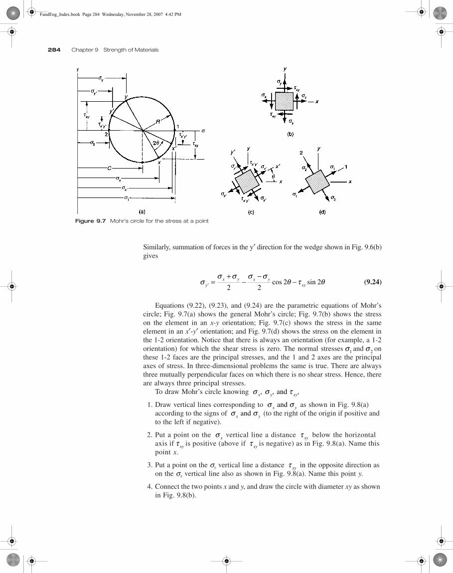
Equations (9.22), (9.23), and (9.24) are the parametric equations of Mohr’scircle; Fig. 9.7(a) shows the general Mohr’s circle; Fig. 9.7(b) shows the stresson the element in an x-y orientation; Fig. 9.7(c) shows the stress in the sameelement in an x′-y′ orientation; and Fig. 9.7(d) shows the stress on the element inthe 1-2 orientation. Notice that there is always an orientation (for example, a 1-2orientation) for which the shear stress is zero. The normal stresses and onthese 1-2 faces are the principal stresses, and the 1 and 2 axes are the principalaxes of stress. In three-dimensional problems the same is true. There are alwaysthree mutually perpendicular faces on which there is no shear stress. Hence, thereare always three principal stresses.
To draw Mohr’s circle knowing
1. Draw vertical lines corresponding to as shown in Fig. 9.8(a) according to the signs of (to the right of the origin if positive and to the left if negative).
2. Put a point on the vertical line a distance below the horizontal axis if is positive (above if is negative) as in Fig. 9.8(a). Name this point x.
3. Put a point on the sy vertical line a distance in the opposite direction as on the sx vertical line also as shown in Fig. 9.8(a). Name this point y.
4. Connect the two points x and y, and draw the circle with diameter xy as shown in Fig. 9.8(b).
Figure 9.7 Mohr’s circle for the stress at a point
σσ σ σ σ
θ τ θ′ =+
−−
−yx y x y
xy2 22 2cos sin
σ1 σ 2
σ σ τx y xy, , , and
σ σx y and σ σx y and
σ x τ xy
τ xy τ xy
τ xy
FundEng_Index.book Page 284 Wednesday, November 28, 2007 4:42 PM

Plane Stress 285
Upon constructing Mohr’s circle you can now rotate the xy diameter throughan angle of 2q to a new position x′y′, which can determine the stress on any faceat that point in the body as shown in Fig. 9.7. Note that rotations of 2q on Mohr’scircle correspond to q in the physical plane; also note that the direction of rotationis the same as in the physical plane (that is, if you go clockwise on Mohr’s circle,the rotation is also clockwise in the physical plane). The construction can also beused to find the principal stresses and the orientation of the principal axes.
Problems involving stress transformations can be solved with Eqs. (9.22),(9.23), and (9.24), from construction of Mohr’s circle, or from some combination.As an example of a combination, it can be seen that the center of Mohr’s circlecan be represented as
(9.25)
The radius of the circle is
(9.26)
The principal stresses then are
(9.27)
Example 9.7Given Find the principle stresses andtheir orientation.
Solution
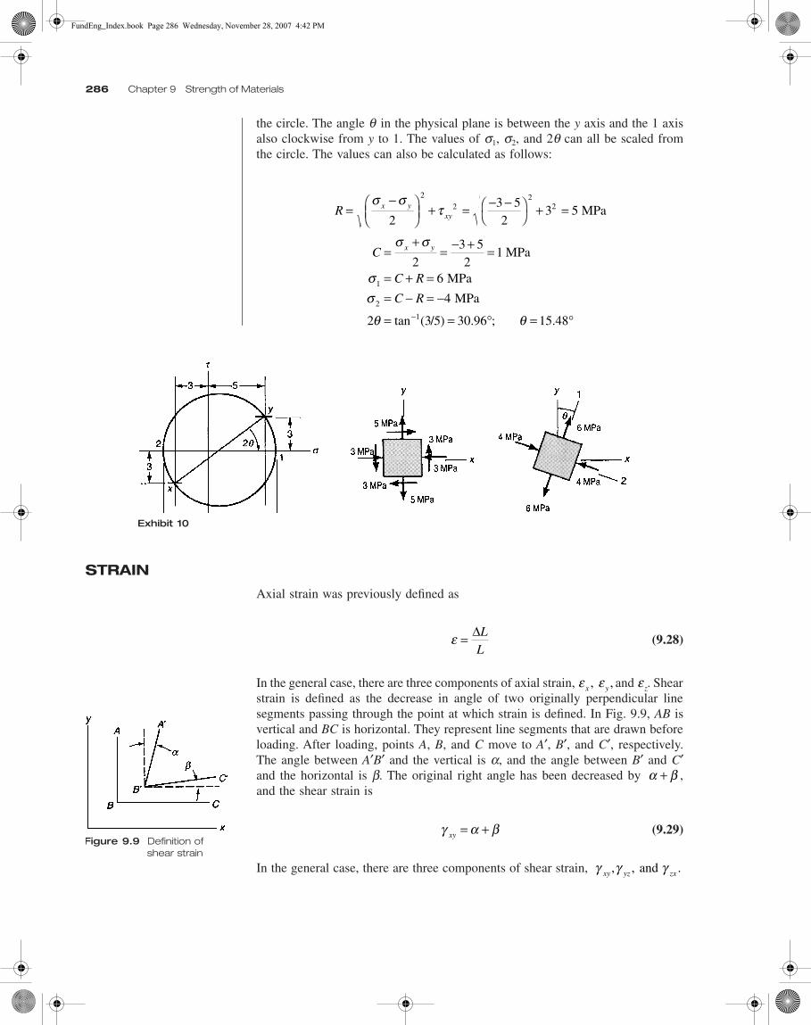
Mohr’s circle is constructed as shown in Exhibit 10. The angle 2q was chosen asthe angle between the y axis and the 1 axis clockwise from y to 1 as shown in
Figure 9.8 Constructing Mohr’s circle
C x y=+σ σ2
R x yxy=
−
+σ σ
τ2
2
2
σ σ1 2= + = −C R C R;
σ σ τx y xy= − = =3 5 3 MPa; MPa; MPa.
FundEng_Index.book Page 285 Wednesday, November 28, 2007 4:42 PM
286 Chapter 9 Strength of Materials
the circle. The angle q in the physical plane is between the y axis and the 1 axisalso clockwise from y to 1. The values of s1, s2, and 2q can all be scaled fromthe circle. The values can also be calculated as follows:
STRAIN
Axial strain was previously defined as
(9.28)
In the general case, there are three components of axial strain, and . Shearstrain is defined as the decrease in angle of two originally perpendicular linesegments passing through the point at which strain is defined. In Fig. 9.9, AB isvertical and BC is horizontal. They represent line segments that are drawn beforeloading. After loading, points A, B, and C move to A′, B′, and C′, respectively.The angle between A′B′ and the vertical is a, and the angle between B′ and C′and the horizontal is b. The original right angle has been decreased by ,and the shear strain is
(9.29)
In the general case, there are three components of shear strain,
R x yxy=
−
+ = − −
+ =
σ στ
23 52
3 52
22
2 MPa
C
C R
C R
x y=+
= − + =
= + == − = −
= = ° = °−
σ σ
σσ
θ θ
23 52
1
6
4
3 5 30 96 15 48
1
MPa
MPa
MPa
2 tan
2
1( / ) . ; .
Exhibit 10
ε = ∆LL
ε εx y, , ε z
Figure 9.9 Definition of shear strain
α β+
γ α βxy = +
γ γ γxy yz zx, , . and
FundEng_Index.book Page 286 Wednesday, November 28, 2007 4:42 PM
Strain 287
Plane Strain
In two dimensions, strain undergoes a similar rotation transformation as stress.The transformation equations are
(9.30)
(9.31)
(9.32)
These equations are the same as Eq. (9.22), (9.23), and (9.24) for stress, exceptthat the has been replaced with with y , and Therefore,Mohr’s circle for strain is treated the same way as that for stress, except for thefactor of two on the shear strain.
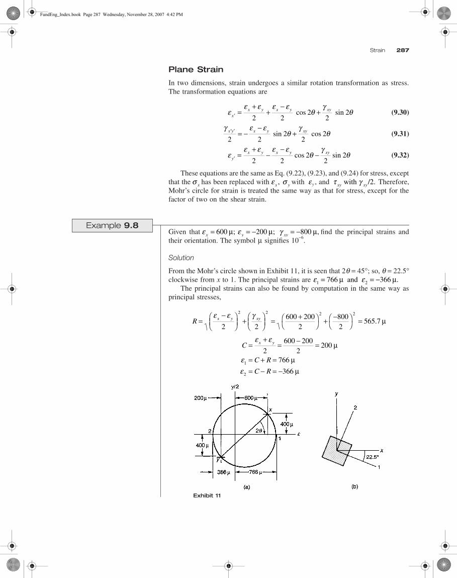
Example 9.8 Given that find the principal strains andtheir orientation. The symbol µ signifies 10−6.
Solution
From the Mohr’s circle shown in Exhibit 11, it is seen that 2q = 45°; so, q = 22.5°clockwise from x to 1. The principal strains are
The principal strains can also be found by computation in the same way asprincipal stresses,
εε ε ε ε
θγ
θ′ =+
+−
+xx y x y xy
2 22
22cos sin
γ ε εθ
γθ′ ′ = −
−+x y x y xy
2 22
22sin cos
εε ε ε ε
θγ
θ′ =+
−−
−yx y x y xy
2 22
22cos sin
σ x ε σx y, ε τ γxy xy with / .2
Exhibit 11
ε ε γx y xy= = − = −600 200 800µ µ µ; ; ,
ε ε1 2766 366= = −µ µ and .
R x y xy=−
+
= +
+ −
=
ε ε γ2 2
600 2002
8002
565 72 2 2 2
. µ
C
C R
C R
x y=+
= − =
= + == − = −
ε ε
εε
2600 200
2200
766
3661
2
µ
µµ
FundEng_Index.book Page 287 Wednesday, November 28, 2007 4:42 PM

288 Chapter 9 Strength of Materials
HOOKE’S LAW
The relationship between stress and strain is expressed by Hooke’s Law. For anisotropic material it is
(9.33)
(9.34)
(9.35)
(9.36)
(9.37)
(9.38)
Further, there is a relationship between E, G, and v which is
(9.39)
Thus, for an isotropic material there are only two independent elastic con-stants. An isotropic material is one that has the same material properties in alldirections. Notable exceptions to isotropy are wood- and fiber-reinforced com-posites.
Example 9.9A steel plate in a state of plane stress is known to have the following strains:
If E = 210 GPa and v = 0.3, what are thestress components, and what is the strain
Solution
In a state of plane stress, the stresses sz = 0, txz = 0 and tyz = 0. From Hooke’s law,
Inverting these relations gives
Mpa
Mpa
From Hooke’s law, the strain gxy is
= 32.3 MPa
ε σ σ σx x y zEv v= − −1
( )
ε σ σ σy y z xEv v= − −1
( )
ε σ σ σz z x yEv v= − −1
( )
γ τxy xyG= 1
γ τyz yzG= 1
γ τzx zxG= 1
GE
v=
+2 1( )
ε ε γx y xy= = =650 250 400µ µ µ, , . and ε z?
ε σ νσx x yE= − −1
0( )
ε σ νσy y xE= − −1
0( )
σν
ε νεx x y
E=−
+ =−
+ =1
210650 0 3 250 167 32 ( ) [ . ( )] .
GPa1 0.32 µ µ
σν
ε νεy y x
E=−
+ =−
+ =1
210250 0 3 650 102 72 ( ) [ . ( )] .
GPa1 0.32 µ µ
γτ
τγ
xyxy
xyxy
GG
Ev
E
v= =
+=
+=
+;
( );
( )(
( . )2 1 2 1210
2 1 0 3 GPa) (400 )µ
FundEng_Index.book Page 288 Wednesday, November 28, 2007 4:42 PM

Torsion 289
The strain in the z direction is
TORSION
Torsion refers to the twisting of long members. Torsion can occur with membersof any cross-sectional shape, but the most common is the circular shaft. Anotherfairly common shaft configuration, which has a simple solution, is the hollow,thin-walled shaft.
Circular Shafts
Fig. 9.10(a) shows a circular shaft before loading; the r-q-z cylindrical coordinatesystem is also shown. In addition to the outline of the shaft, two longitudinal lines,two circumferential lines, and two diametral lines are shown scribed on the shaft.These lines are drawn to show the deformed shape loading. Fig. 9.10(b) showsthe shaft after loading with a torque T. The double arrow notation on T indicatesa moment about the z axis in a right-handed direction. The effect of the torsionis that each cross-section remains plane and simply rotates with respect to othercross-sections. The angle f is the twist of the shaft at any position z. The rotationf(z) is in the q direction.
The distance b shown in Fig. 9.10(b) can be expressed as b = fr or as b = g z.The shear strain for this special case can be expressed as
(9.40)
For the general case where f is not a linear function of z the shear strain can beexpressed as
(9.41)
df/dz is the twist per unit length or the rate of twist.
ε σ σ σ σz x y x yEv v
vE
= − − = − +
= − + = −
10
0 3210
167 3
( ) ( )
.( .
GPa MPa 102.7 MPa) 386 µ
γ φφz r
z=
γ φφz r
d
dz=
Figure 9.10 Torsion in a circular shaft
FundEng_Index.book Page 289 Wednesday, November 28, 2007 4:42 PM

290 Chapter 9 Strength of Materials
The application of Hooke’s Law gives
(9.42)
The torque at the distance z along the shaft is found by summing the contributionsof the shear stress at each point in the cross-section by means of an integration
(9.43)
where J is the polar moment of inertia of the circular cross-section. For a solidshaft with an outer radius of ro the polar moment of inertia is
(9.44)
For a hollow circular shaft with outer radius ro and inner radius ri, the polarmoment of inertia is
(9.45)
Note that the J that appears in Eq. (9.43) is the polar moment of inertia only forthe special case of circular shafts (either solid or hollow). For any other cross-section shape, Eq. (9.43) is valid only if J is redefined as a torsional constant notequal to the polar moment of inertia. Eq. (9.42) can be combined with Eq. (9.43)to give
(9.46)
The maximum shear stress occurs at the outer radius of the shaft and at the locationalong the shaft where the torque is maximum.
(9.47)
The angle of twist of the shaft can be found by integrating Eq. (9.43)
(9.48)
For a uniform circular shaft with a constant torque along its length, this equationbecomes
(9.49)
Example 9.10The hollow circular steel shaft shown in Exhibit 12 has an inner diameter of25 mm, an outer diameter of 50 mm, and a length of 600 mm. It is fixed at theleft end and subjected to a torque of 1400 N • m as shown in Exhibit 12. Findthe maximum shear stress in the shaft and the angle of twist at the right end. TakeG = 84 GPa.
τ γ φφ φz zG Gr
d
dz= =
T r dA Gddz
r dA GJddzz
AA= = =∫∫ τ φ φ
φ 2
Jro=
π 4
2
J r ro i= −( )π2
4 4
τ φz
Tr
J=
τ φzoT r
J maxmax=
φ = ∫ T
GJdz
L
0
φ = TL
GJ
FundEng_Index.book Page 290 Wednesday, November 28, 2007 4:42 PM

Torsion 291
Solution
Hollow, Thin-Walled Shafts
In hollow, thin-walled shafts, the assumption is made that the shear stress τsz isconstant throughout the wall thickness t. The shear flow q is defined as the productof τsz and t. From a summation of forces in the z direction, it can be shown thatq is constant—even with varying thickness. The torque is found by summing thecontributions of the shear flow. Fig. 9.11 shows the cross-section of the thin-walledtube of nonconstant thickness. The z coordinate is perpendicular to the plane ofthe paper. The shear flow q is taken in a counter-clockwise sense. The torqueproduced by q over the element ds is
d T = qr ds
The total torque is, therefore,
(9.50)
The area dA is the area of the triangle of base ds and height r,
dA = (base)(height) = (9.51)
Exhibit 12
Figure 9.11 Cross-section of thin-walled tube
J r r= −( ) = − = ×π π2 2
25 12 5 575 104 4 3 4o i [( ( . ] mm) mm) mm4 4
τθz
T r
J maxmax
4
N m)(25 mm)mm
MPa= = •×
=o (.
1400575 10
60 83
φ = = •×
=TLGJ
(( )
.1400
84 575 100 017383
N m)(600 mm) GPa)( mm
rad4
T qr ds q r ds= =∫ ∫
12
r ds
2
Chapter 09.fm Page 291 Wednesday, March 12, 2008 9:17 AM

292 Chapter 9 Strength of Materials
so that
(9.52)
where Am is the area enclosed by the wall (including the hole). It is best to usethe centerline of the wall to define the boundary of the area, hence Am is the meanarea. The expression for the torque is
T = 2Amq (9.53)
and from the definition of q the shear stress can be expressed as
(9.54)
Example 9.11A torque of 10 kN • m is applied to a thin-walled rectangular steel shaft whosecross-section is shown in Exhibit 13. The shaft has wall thicknesses of 5 mm and10 mm. Find the maximum shear stress in the shaft.
Solution
Am = (200 − 5)(300 − 10) = 56,550 mm2
The maximum shear stress will occur in the thinnest section, so t = 5 mm.
BEAMS
Shear and Moment Diagrams
Shear and moment diagrams are plots of the shear forces and bending moments,respectively, along the length of a beam. The purpose of these plots is to clearlyshow maximums of the shear force and bending moment, which are important inthe design of beams. The most common sign convention for the shear force andbending moment in beams is shown in Fig. 9.12. One method of determining theshear and moment diagrams is by the following steps:
1. Determine the reactions from equilibrium of the entire beam.
2. Cut the beam at an arbitrary point.
r ds Am∫ = 2
τ szm
TA t
=2
Exhibit 13
τ szm
TA t
= = • =2
102 56 550 5
17 68 2
kN mmm mm)
MNm2( , )(
.
FundEng_Index.book Page 292 Wednesday, November 28, 2007 4:42 PM
Beams 293
3. Show the unknown shear and moment on the cut using the positive sign convention shown in Fig. 9.12.
4. Sum forces in the vertical direction to determine the unknown shear.
5. Sum moments about the cut to determine the unknown moment.
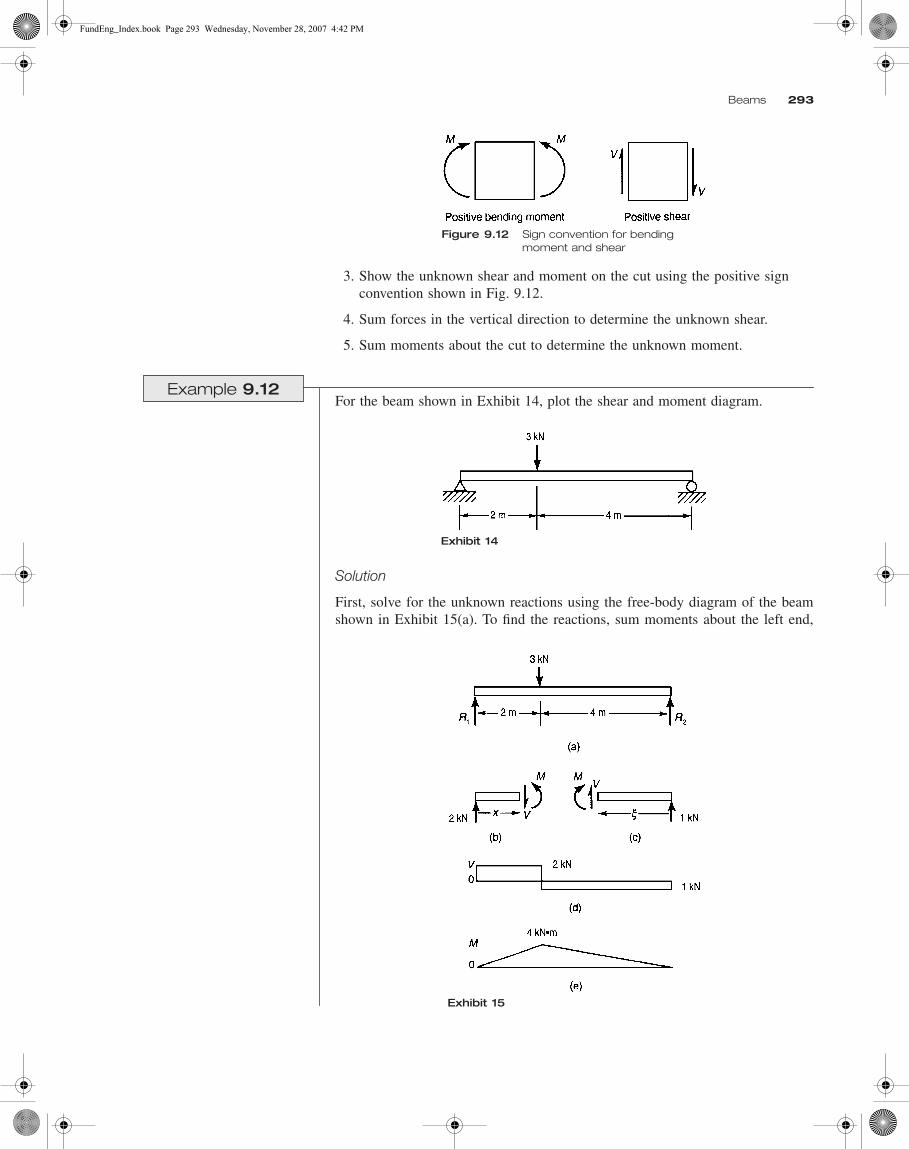
Example 9.12 For the beam shown in Exhibit 14, plot the shear and moment diagram.
Solution
First, solve for the unknown reactions using the free-body diagram of the beamshown in Exhibit 15(a). To find the reactions, sum moments about the left end,
Figure 9.12 Sign convention for bending moment and shear
Exhibit 14
Exhibit 15
FundEng_Index.book Page 293 Wednesday, November 28, 2007 4:42 PM

294 Chapter 9 Strength of Materials
which gives
6R2 − (3)(2) = 0 or R2 = 6/6 = 1 kN
Sum forces in the vertical direction to get
R1 + R2 = 3 = R1 + 1 or R1 = 2 kN
Cut the beam between the left end and the load as shown in Exhibit 15(b). Showthe unknown moment and shear on the cut using the positive sign conventionshown in Fig. 9.12. Sum the vertical forces to get
V = 2 kN (independent of x)
Sum moments about the cut to get
M = R1x = 2x
Repeat the procedure by making a cut between the right end of the beam and the3-kN load, as shown in Exhibit 15(c). Again, sum vertical forces and sum momentsabout the cut to get
V = 1 kN (independent of x ), and M = 1x
The plots of these expressions for shear and moment give the shear and momentdiagrams shown in Exhibit 15(d) and 15(e).
It should be noted that the shear diagram in this example has a jump at thepoint of the load and that the jump is equal to the load. This is always the case.Similarly, a moment diagram will have a jump equal to an applied concentratedmoment. In this example, there was no concentrated moment applied, so themoment was everywhere continuous.
Another useful way of determining the shear and moment diagram is by usingdifferential relationships. These relationships are found by considering an elementof length ∆ x of the beam. The forces on that element are shown in Fig. 9.13.Summation of forces in the y direction gives
(9.55)
which gives
(9.56)
Figure 9.13
q x V VdVdx
x∆ ∆+ − − = 0
dV
dxq=
FundEng_Index.book Page 294 Wednesday, November 28, 2007 4:42 PM

Beams 295
Summing moments and neglecting higher order terms gives
−M + M + (9.57)
which gives
(9.58)
Integral forms of these relationships are expressed as
(9.59)
(9.60)
Example 9.13The simply supported uniform beam shown in Exhibit 16 carries a uniform loadof w0 . Plot the shear and moment diagrams for this beam.
Solution
As before, the reactions can be found first from the free-body diagram of the beamshown in Exhibit 17(a). It can be seen that, from symmetry, R1 = R2. Summingvertical forces then gives
dMdx
x V x∆ ∆− = 0
dM
dxV=
V V q dxx
x
2 11
2
− = ∫M M V dx
x
x
2 11
2
− = ∫
Exhibit 16
Exhibit 17
R R Rw L
= = =1 20
2
FundEng_Index.book Page 295 Wednesday, November 28, 2007 4:42 PM

296 Chapter 9 Strength of Materials
The load q = −w0, so Eq. (9.59) reads
Noting that the moment at x = 0 is zero, Eq. (9.60) gives
It can be seen that the shear diagram is a straight line, and the moment variesparabolically with x. Shear and moment diagrams are shown in Exhibit 17(b) andExhibit 17(c). It can be seen that the maximum bending moment occurs at the centerof the beam where the shear stress is zero. The maximum bending moment alwayshas a relative maximum at the place where the shear is zero because the shear isthe derivative of the moment, and relative maxima occur when the derivative is zero.
Often it is helpful to use a combination of methods to find the shear andmoment diagrams. For instance, if there is no load between two points, then theshear diagram is constant, and the moment diagram is a straight line. If there is auniform load, then the shear diagram is a straight line, and the moment diagram isparabolic. The following example illustrates this method.
Example 9.14Draw the shear and moment diagrams for the beam shown in Exhibit 18(a).
Solution
Draw the free-body diagram of the beam as shown in Exhibit 18(b). From a sum-mation of the moments about the right end,
From a summation of forces in the vertical direction,
V V w dxw L
w xx
= − = −∫0 00
002
M Mw L
w x dxw Lx w x w x
L xx
= − −
= + − = −∫0
00
0
0 02
0
20
2 2 2
( )
10 4 7 3 2 34 3 41 1R R= + = =( )( ) ( )( ) ; .so kN
R2 7 3 4 3 6= − =. . kN
Exhibit 18
FundEng_Index.book Page 296 Wednesday, November 28, 2007 4:42 PM
Beams 297
The shear in the left portion is 3.4 kN, the shear in the right portion is −3.6 kNand the shear in the center portion is 3.4 − 4 = −0.6 kN. This is sufficientinformation to draw the shear diagram shown in Exhibit 18(c). The moment at Ais zero, so the moment at B is the shaded area A1 and the moment at C is A1 − A2.
The moments at A and D are zero, and the moment diagram consists of straightlines between the points A, B, C, and D. There is, therefore, enough informationto plot the moment diagram shown in Exhibit 18(d).
Stresses in Beams
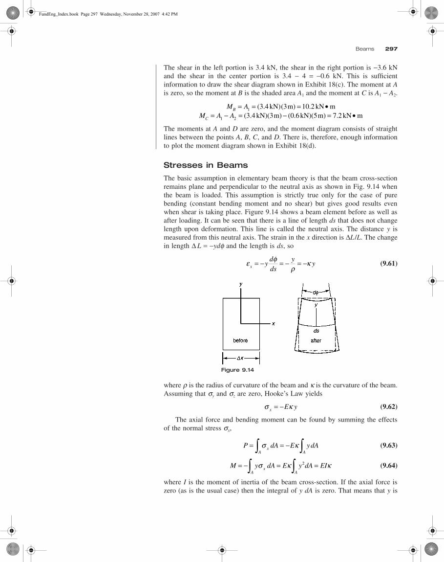
The basic assumption in elementary beam theory is that the beam cross-sectionremains plane and perpendicular to the neutral axis as shown in Fig. 9.14 whenthe beam is loaded. This assumption is strictly true only for the case of purebending (constant bending moment and no shear) but gives good results evenwhen shear is taking place. Figure 9.14 shows a beam element before as well asafter loading. It can be seen that there is a line of length ds that does not changelength upon deformation. This line is called the neutral axis. The distance y ismeasured from this neutral axis. The strain in the x direction is ∆L /L. The changein length ∆ L = −ydf and the length is ds, so
(9.61)
where r is the radius of curvature of the beam and k is the curvature of the beam.Assuming that sy and sz are zero, Hooke’s Law yields
(9.62)
The axial force and bending moment can be found by summing the effectsof the normal stress sx,
(9.63)
(9.64)
where I is the moment of inertia of the beam cross-section. If the axial force iszero (as is the usual case) then the integral of y dA is zero. That means that y is
Figure 9.14
M AM A A
B
C
= = = •= − = − = •
1
1 2
3 43
( .( .
kN)(3m) 10.2 kN m4 kN)(3m) (0.6kN)(5m) 7.2 kN m
ε φρ
κx ydds
yy= − = − = −
σ κx E y= −
P dA E ydAxA A
= = −∫ ∫σ κ
M y dA E y dA EIxA A
= − = =∫ ∫σ κ κ2
FundEng_Index.book Page 297 Wednesday, November 28, 2007 4:42 PM
298 Chapter 9 Strength of Materials
measured from the centroidal axis of the cross-section. Since y is also measuredfrom the neutral axis, the neutral axis coincides with the centroidal axis. FromEq. (9.62) and (9.64), the bending stress sx can be expressed as
(9.65)
The maximum bending stress occurs where the magnitude of the bendingmoment is a maximum and at the maximum distance from the neutral axis. Forsymmetrical beam sections the value of ymax = ±C where C is the distance to theextreme fiber so the maximum stress is
(9.66)
where S is the section modulus (S = I/C).
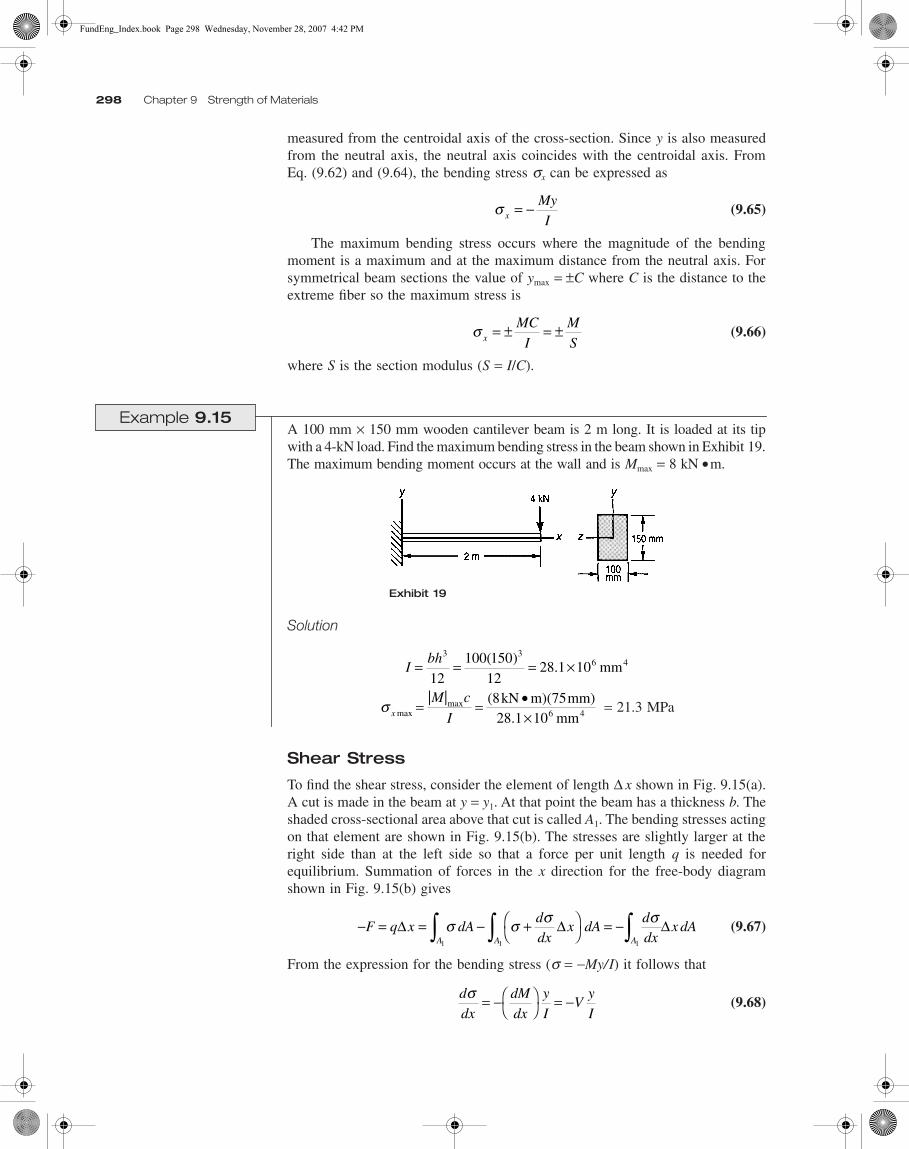
Example 9.15A 100 mm × 150 mm wooden cantilever beam is 2 m long. It is loaded at its tipwith a 4-kN load. Find the maximum bending stress in the beam shown in Exhibit 19.The maximum bending moment occurs at the wall and is Mmax = 8 kN • m.
Solution
= 21.3 MPa
Shear Stress
To find the shear stress, consider the element of length ∆ x shown in Fig. 9.15(a).A cut is made in the beam at y = y1. At that point the beam has a thickness b. Theshaded cross-sectional area above that cut is called A1. The bending stresses actingon that element are shown in Fig. 9.15(b). The stresses are slightly larger at theright side than at the left side so that a force per unit length q is needed forequilibrium. Summation of forces in the x direction for the free-body diagramshown in Fig. 9.15(b) gives
(9.67)
From the expression for the bending stress (s = −My/I) it follows that
(9.68)
σ x
My
I= −
σ x
MC
I
M
S= ± = ±
Exhibit 19
Ibh= = = ×
3 36 4
12100 150
1228 1 10
( ). mm
σ x
M c
Imaxmax| |
= = •×
(8kN m)(75mm)28.1 10 mm6 4
− = = − +
= −∫ ∫ ∫F q x dA
ddx
x dAddx
x dAA A A
∆ ∆ ∆σ σ σ σ1 1 1
d
dx
dM
dx
y
IV
y
I
σ = −
= −
FundEng_Index.book Page 298 Wednesday, November 28, 2007 4:42 PM

Beams 299
Substituting Eq. (9.68) into Eq. (9.67) gives
(9.69)
If the shear stress t is assumed to be uniform over the thickness b then t = q/band the expression for shear stress is
(9.70)
where V is the shear in the beam, Q is the moment of area above (or below) thepoint in the beam at which the shear stress is sought, I is the moment of inertiaof the entire beam cross-section, and b is the thickness of the beam cross-sectionat the point where the shear stress is sought. The definition of Q from Eq. (9.69) is
(9.71)
Example 9.16The cross-section of the beam shown in Exhibit 20 has an applied shear of 10 kN.Find (a) the shear stress at a point 20 mm below the top of the beam and (b) themaximum shear stress from the shear force.
Solution
The section is divided into two parts by the dashed line shown in Exhibit 21(a).The centroids of each of the two sections are also shown in Exhibit 21(a). Thecentroid of the entire cross-section is found as follows
Figure 9.15 Shear stress in beams
qV
Iy dA
VQ
IA= =∫
1
τ = VQ
Ib
Q y dA A yA
= =∫1
1
Exhibit 20y
y A
A
n n
n
N
n
n
N= = + ++
==
=
∑∑
1
1
60 20 30 20 80 20 1060 20 80 20
27 14( )( )( ) ( )( )( )
( )( ) ( )( ). mm (from bottom)
FundEng_Index.book Page 299 Wednesday, November 28, 2007 4:42 PM
300 Chapter 9 Strength of Materials
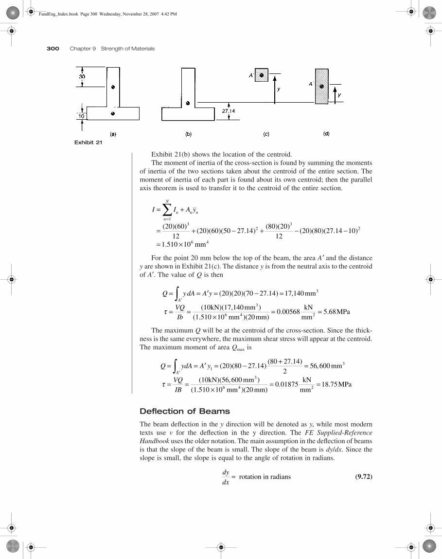
Exhibit 21(b) shows the location of the centroid.The moment of inertia of the cross-section is found by summing the moments
of inertia of the two sections taken about the centroid of the entire section. Themoment of inertia of each part is found about its own centroid; then the parallelaxis theorem is used to transfer it to the centroid of the entire section.
For the point 20 mm below the top of the beam, the area A′ and the distancey are shown in Exhibit 21(c). The distance y is from the neutral axis to the centroidof A′. The value of Q is then
The maximum Q will be at the centroid of the cross-section. Since the thick-ness is the same everywhere, the maximum shear stress will appear at the centroid.The maximum moment of area Qmax is
Deflection of Beams
The beam deflection in the y direction will be denoted as y, while most moderntexts use v for the deflection in the y direction. The FE Supplied-ReferenceHandbook uses the older notation. The main assumption in the deflection of beamsis that the slope of the beam is small. The slope of the beam is dy/dx. Since theslope is small, the slope is equal to the angle of rotation in radians.
(9.72)
Exhibit 21
I I A yn
n
N
n n= +
= + − + − −
= ×
=∑
13
23
2
6 4
20 6012
20 60 50 27 1480 20
1220 80 27 14 10
1 510 10
( )( )( )( )( . )
( )( )( )( )( . )
. mm
Q ydA A y
VQIb
A= = ′ = − =
= =×
= =
′∫ ( )( )( . ) ,20 20 70 27 14 17 140 3mm
(10kN)(17,140mm )(1.510 10 mm )(20mm)
0.00568kN
mm5.68MPa
3
6 4 2τ
Q ydA A y
VQ
IB
A= = ′ = − + =
= =×
= =
′∫ 1 20 80 27 1480 27 14
256 600( )( . )
( . ), mm
(10kN)(56,600 mm )(1.510 10 mm )(20 mm)
0.01875kN
mm18.75MPa
3
3
6 4 2τ
dy
dx= rotation in radians
FundEng_Index.book Page 300 Wednesday, November 28, 2007 4:42 PM
Beams 301
Because the slope is small it also follows that
(9.73)
From Eq. (9.62) this gives
(9.74)
This equation, together with two boundary conditions, can be used to find thebeam deflection. Integrating twice with respect to x gives
(9.75)
(9.76)
where the constants C1 and C2 are determined from the two boundary conditions.Appropriate boundary conditions are on the displacement y or on the slope dy/dx.In the common problems of uniform beams, the beam stiffness EI is a constantand can be removed from beneath the integral sign.
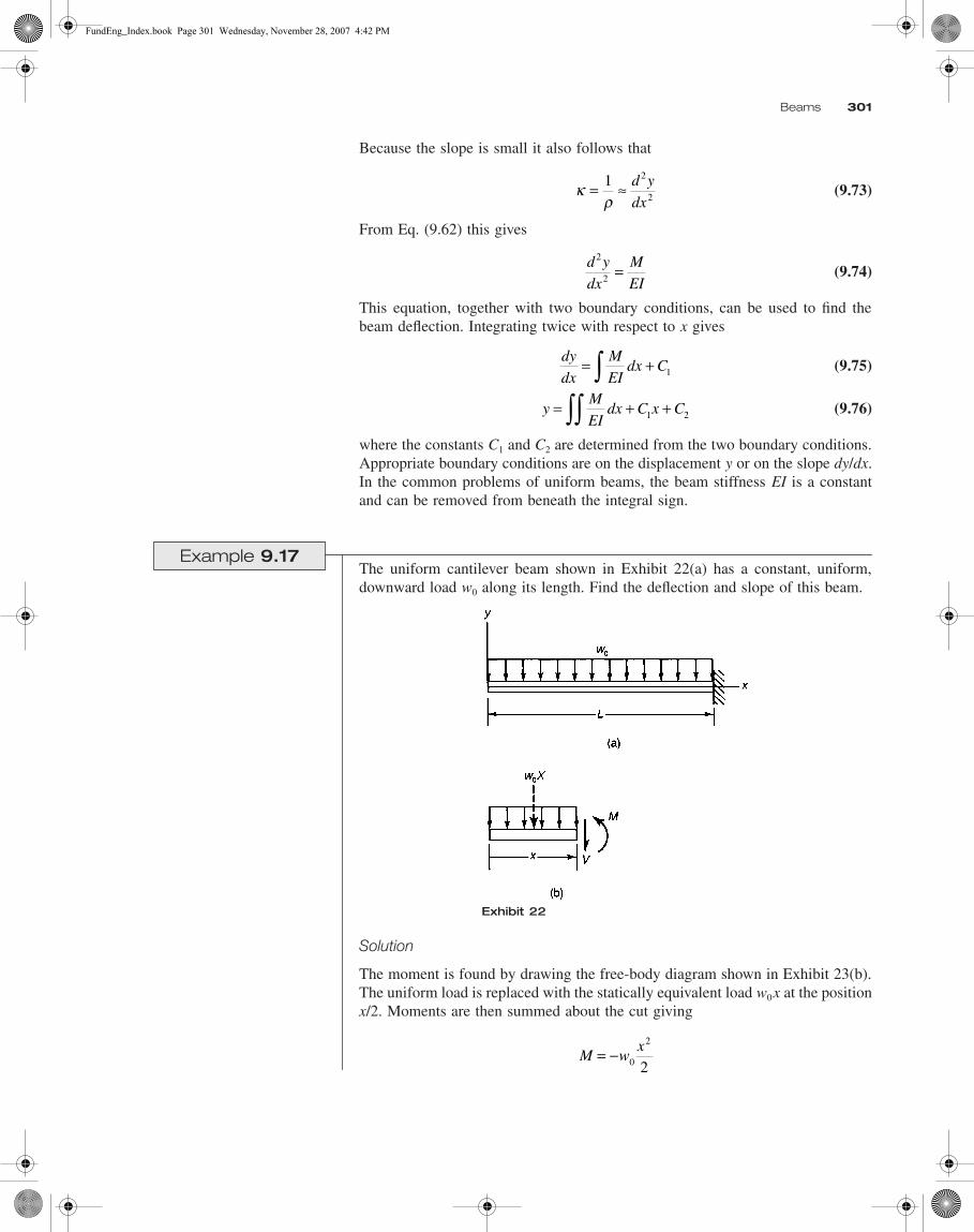
Example 9.17The uniform cantilever beam shown in Exhibit 22(a) has a constant, uniform,downward load w0 along its length. Find the deflection and slope of this beam.
Solution
The moment is found by drawing the free-body diagram shown in Exhibit 23(b).The uniform load is replaced with the statically equivalent load w0x at the positionx/2. Moments are then summed about the cut giving
κρ
= ≈1 2
2
d y
dx
d y
dx
M
EI
2
2 =
dy
dx
M
EIdx C= +∫ 1
yM
EIdx C x C= + +∫∫ 1 2
Exhibit 22
M wx= − 0
2
2
FundEng_Index.book Page 301 Wednesday, November 28, 2007 4:42 PM

302 Chapter 9 Strength of Materials
Integrating twice with respect to x,
At x = L the displacement and slope must be zero so that
Therefore,
Inserting C1 and C2 into the previous expressions gives
Fourth-Order Beam Equation
The second-order beam Eq. (9.74) can be combined with the differential relation-ships between the shear, moment, and distributed load. Differentiate Eq. (9.74)with respect to x, and use Eq. (9.58).
(9.77)
Differentiate again with respect to x and use Eq. (9.56).
(9.78)
For a uniform beam (that is, constant EI ) the fourth-order beam equation becomes
(9.79)
This equation can be integrated four times with respect to x. Four boundaryconditions are required to solve for the four constants of integration. The boundary
dy
dx
M
EIdx C
EIw
xdx C
w x= + = −
+ = −∫1 0
2
101
216
33
1
03
1 2
16
124
EIC
yw x
EIdx C x C
w
∫ +
= −
+ + = − 00
4
1 2
x
EIC x C∫ + +
y Lw L
EIC L C
dy
dxL
w L
EI
( )
( )
= = − + +
= = −
01
24
016
04
1 2
03
++ C1
Cw L
EIC
w L
EI10
3
20
416
18
= = −;
yw
EIx xL L= − − +0 4 3 4
244 3( )
dy
dx
w
EIL x= −0 3 3
6( )
ddx
EId ydx
dMdx
V2
2
= =
d
dxEI
d y
dx
dV
dxq
2
2
2
2
= =
EId y
dxq
4
4 =
FundEng_Index.book Page 302 Wednesday, November 28, 2007 4:42 PM
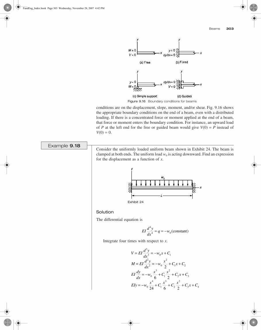
Beams 303
conditions are on the displacement, slope, moment, and/or shear. Fig. 9.16 showsthe appropriate boundary conditions on the end of a beam, even with a distributedloading. If there is a concentrated force or moment applied at the end of a beam,that force or moment enters the boundary condition. For instance, an upward loadof P at the left end for the free or guided beam would give V(0) = P instead ofV(0) = 0.
Example 9.18Consider the uniformly loaded uniform beam shown in Exhibit 24. The beam isclamped at both ends. The uniform load w0 is acting downward. Find an expressionfor the displacement as a function of x.
Solution
The differential equation is
Integrate four times with respect to x.
Figure 9.16 Boundary conditions for beams
Exhibit 24
EId y
dxq w
4
4 0= = − ( )constant
V EId y
dxw x C
M EId y
dxw
xC x C
EIdy
dxw
xC
xC x C
EIy wx
Cx
Cx
C x C
= = − +
= = − + +
= − + + +
= − + + + +
3
3 0 1
2
2 0
2
1 2
0
3
1
2
2 3
0
4
1
3
2
2
3 4
2
6 2
24 6 2
FundEng_Index.book Page 303 Wednesday, November 28, 2007 4:42 PM

304 Chapter 9 Strength of Materials
The four constants of integration can be found from four boundary conditions.The boundary conditions are
These lead to the following:
Solving the last two equations for C1 and C2 gives
Inserting these values into the equation for y gives
Some solutions for uniform beams with various loads and boundary conditionsare shown in Table 9.1.
ydy
dxy L
dy
dxL( ) ; ( ) ; ( ) ; ( )0 0 0 0 0 0= = = =
EIy C
EIdydx
C
EIy L wL
CL
CL
EIdydx
L wL
CL
C L
( )
( )
( )
( )
0 0
0 0
024 6 2
06 2
4
3
0
4
1
3
2
2
0
3
1
2
2
= =
= =
= = − + +
= = − + +
C w L C w L1 0 2 021
21
12= = −;
yw x
EIx xL L= − − +
02
2 2124
112
124
Table 9.1 Deflection and slope formulas for beams
Beam Deflection, v Slope, v′
1. For 0 x a
For a x L
For 0 x a
For a x L
2.
3. For 0 x a
For a x L
For 0 x a
For a x L
4.
≤ ≤
yPx
EIa x= −
2
63( )
≤ ≤
yPa
EIx a= −
2
63( )
≤ ≤dydx
pxEI
a x= −2
2( )
≤ ≤
dydx
PaEI
a=2
2
yw x
EIx Lx L= − − +0
22 2
244 6( )
dydx
w x
EIx Lx L= − − +0 2 2
612 12( )
≤ ≤
yPbxLEI
L b x= − −6
2 2 2( )
≤ ≤
yPa L x
LEILx a x= − − −( )
( )6
2 2 2
≤ ≤dydx
PbLEI
L b x= − −6
32 2 2( )
≤ ≤dydx
PaLEI
L a Lx x= + − +6
2 6 32 2 2( )
yw x
EIL Lx x= − − +0 3 2 3
242( )
dydx
w
EIL Lx x= − − +0 3 2 3
246 4( )
FundEng_Index.book Page 304 Wednesday, November 28, 2007 4:42 PM
Beams 305
Superposition
In addition to the use of second-order and fourth-order differential equations, avery powerful technique for determining deflections is the use of superposition.Because all of the governing differential equations are linear, solutions can bedirectly superposed. Use can be made of tables of known solutions, such as thosein Table 9.1, to form solutions to many other problems. Some examples of super-position follow.
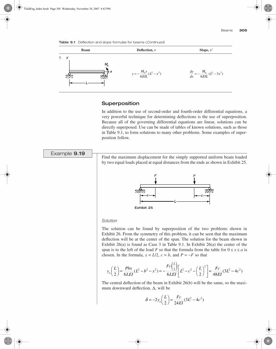
Example 9.19Find the maximum displacement for the simply supported uniform beam loadedby two equal loads placed at equal distances from the ends as shown in Exhibit 25.
Solution
The solution can be found by superposition of the two problems shown inExhibit 26. From the symmetry of this problem, it can be seen that the maximumdeflection will be at the center of the span. The solution for the beam shown inExhibit 26(a) is found as Case 3 in Table 9.1. In Exhibit 26(a) the center of thespan is to the left of the load F so that the formula from the table for 0 x a ischosen. In the formula, x = L/2, c = b, and P = −F so that
The central deflection of the beam in Exhibit 26(b) will be the same, so the maxi-mum downward deflection, ∆, will be
Table 9.1 Deflection and slope formulas for beams (Continued)
Beam Deflection, v Slope, v′
5.
yM x
EILL x= − −0 2 2
6( )
dydx
M
EILL x= − −0 2 2
63( )
Exhibit 25
≤ ≤
yL Pbx
LEIL b x
Fc
LEIL c
L FcEI
L ca
L
2 6 6 2 483 42 2 2 2 2
22 22
= − − = −
( )− −
= −( ) ( )
δ = −
= −2
2 243 42 2y
L FcEI
L ca ( )
FundEng_Index.book Page 305 Wednesday, November 28, 2007 4:42 PM
306 Chapter 9 Strength of Materials
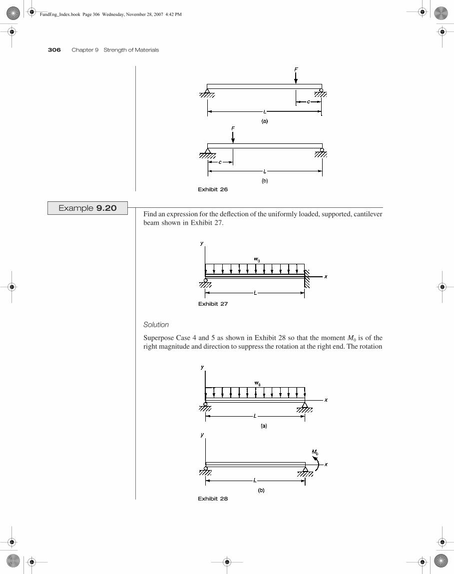
Example 9.20Find an expression for the deflection of the uniformly loaded, supported, cantileverbeam shown in Exhibit 27.
Solution
Superpose Case 4 and 5 as shown in Exhibit 28 so that the moment M0 is of theright magnitude and direction to suppress the rotation at the right end. The rotation
Exhibit 26
Exhibit 27
Exhibit 28
FundEng_Index.book Page 306 Wednesday, November 28, 2007 4:42 PM

Combined Stress 307
for each case from Table 9.1 is
Setting the rotation at the end equal to zero gives
Substituting this expression into the formulas in the table and adding gives
COMBINED STRESS
In many cases, members can be loaded in a combination of bending, torsion, andaxial loading. In these cases, the solution of each portion is exactly as before; theeffects of each are simply added. This concept is best illustrated by an example.
Example 9.21In Exhibit 29, there is a thin-walled, aluminum tube AB, which is attached to awall at A. The tube has a rectangular cross-section member BC attached to it. Avertical load is placed on the member BC as shown. The aluminum tube has anouter diameter of 50 mm and a wall thickness of 3.25 mm. Take P = 900 N, a =450 mm, and b = 400 mm. Find the state of stress at the top of the tube at the pointD. Draw Mohr’s circle for this point, and find the three principal stresses.
dy
dx
w
EIL L L
w L
EI
dy
dx
M
EILL L
M L
EI
x L
x L
= − − + =
= − − =
=
=
4
0 3 3 3 03
5
0 2 2 0
246 4
24
63
3
( )
( )
dy
dx
dy
dx
w L
EI
M L
EI
Mw L
x L x L
+
= = − +
= −
= =4 5
03
0
00
2
024 3
8
yw x
EIL Lx x
w L x
EIL x
w x
EIL Lx x= − − + + − = − − +0 3 2 3 0
22 2 0 3 2 3
242
8 6 483 2( ) ( ) ( )
Exhibit 29
FundEng_Index.book Page 307 Wednesday, November 28, 2007 4:42 PM

308 Chapter 9 Strength of Materials
Solution
Cut the tube at the Point D. Draw the free-body diagram as in Exhibit 30(a). Fromthat free-body diagram, a summation of moments at the cut about the z axis gives
T = Pa = (900 N)(450 mm) = 405 N • m
A summation of moments at the cut about an axis parallel with the x axis gives
Mb = Pb = (900 N)(400 mm) = 360 N • m
A summation of vertical forces gives
V = P
Exhibit 30(b) shows the force and moments acting on the cross-section. Thebending and shearing stresses caused by these loads are
The shearing stress attributed to V will be zero at the top of the beam and canbe neglected. The moments of inertia are
At the top of the tube r = 25 mm and y = 25 mm, so the stresses are
Exhibit 30
σ
τ
τ
θ
θ
zb
xxb
zz
zxx
M y
IM
TrI
T
VQI b
V
=
=
=
( )
( )
( )
from
from
from
Ir r
Ir r
I
xxo i
zo i
xx
=−( )
= − = ×
=−( )
= = ×
π π
π
4 4 4 43 4
4 43 4
425 21 75
4131 10
22 262 10
( . )mm
mm
σ
τ θ
zb
xx
zz
M y
I
TrI
= = •×
=
= = •×
=
( )( ).
360 25131 10
68 73 4
N m mmmm
MPa
(405 N m)(25mm)262 10 mm
38.6 MPa3 4
FundEng_Index.book Page 308 Wednesday, November 28, 2007 4:42 PM

Columns 309
The Mohr’s circle plot for this is shown in Exhibit 31.
Because this is a state of plane stress, the third principal stress is
s3 = 0
COLUMNS
Buckling can occur in slender columns when they carry a high axial load.Fig. 9.17(a) shows a simply supported slender member with an axial load. Thebeam is shown in the horizontal position rather than in the vertical position forconvenience. It is assumed that the member will deflect from its normally straightconfiguration as shown. The free-body diagram of the beam is shown in Fig. 9.17(b).Figure 9.17(c) shows the free-body diagram of a section of the beam. Summationof moments on the beam section in Fig. 9.17(c) yields
M + Py = 0 (9.80)
Since M is equal to EI times the curvature, the equation for this beam can beexpressed as
(9.81)
where
(9.82)
Exhibit 31
R zz=
−
+ = −
+ =
σ στθ
θ268 7 0
238 6 51 7
22
22.
. . MPa
C
C RC R
z= = =
= + == − = −
σ σ
σσ
θ
268 7
234 4
86 117 3
1
2
..
..
MPa
MPaMPa
Figure 9.17 Buckling of simply supported column
d y
dxy
2
2 0+ =λ
λ2 = P
EI
FundEng_Index.book Page 309 Wednesday, November 28, 2007 4:42 PM

310 Chapter 9 Strength of Materials
The solution satisfying the boundary conditions that the displacement is zeroat either end is
v = sin (l x), where l = np/L n = 1, 2, 3… (9.83)
The lowest value for the load P is the buckling load, so n = 1 and the criticalbuckling load, or Euler buckling load, is
(9.84)
For other than simply supported boundary conditions, the shape of the deflectedcurve will always be some portion of a sine curve. The simplest shape consistentwith the boundary conditions will be the deflected shape. Fig. 9.18 shows a sinecurve and the beam lengths that can be selected from the sine curve. The criticalbuckling load can be redefined as
(9.85)
where the radius of gyration r is defined as . The ratio L /r is called theslenderness ratio.
From Fig. 9.18, it can be seen that the values for Le and k are as follows:
For simple supports: L = Le; Le = L; k = 1
For a cantilever: L = 0.5Le; Le = 2L; k = 2
For both ends clamped: L = 2Le; Le = 0.5L; k = 0.5
For supported-clamped: L = 1.43Le; Le = 0.7L; k = 0.7
Figure 9.18 Buckling of columns with various boundary conditions
PEI
Lcr = π 2
2
PEI
LEI
kLE
kL recr = = =π π π2
2
2
2
2
2( ) ( / )
I A/
FundEng_Index.book Page 310 Wednesday, November 28, 2007 4:42 PM

Selected Symbols and Abbreviations 311
In dealing with buckling problems, keep in mind that the member must beslender before buckling is the mode of failure. If the beam is not slender, it willfail by yielding or crushing before buckling can take place.
Example 9.22 A steel pipe is to be used to support a weight of 130 kN as shown in Exhibit 32.The pipe has the following specifications: OD = 100 mm, ID = 90 mm, A = 1500mm2, and I = 1.7 × 106 mm4. Take E = 210 GPa and the yield stress Y = 250 MPa.Find the maximum length of the pipe.
Solution
First, check to make sure that the pipe won’t yield under the applied weight. Thestress is
This stress is well below the yield, so buckling will be the governing mode offailure. This is a cantilever column, so the constant k is 2. The critical load is
Solving for L gives
The maximum length is 2.6 m.
SELECTED SYMBOLS AND ABBREVIATIONS
Exhibit 32
σ = = = <P
AY
1301500
86 72
kNmm
MPa.
PEI
Lcr = π 2
22( )
LEI
P= = × =π π
4(210 GPa)(1.7 10 mm )
4(130 kN)2.60 m
6 4
Symbol or Abbreviation Description
s stress
e strain
v Poisson’s ratio
kip kilopound
E modulus of elasticity
d deformation
W weight
P load
P, p pressure
I moment of inertia
t shear stress
T torque
A area
M moment
V shear
L length
F force
FundEng_Index.book Page 311 Wednesday, November 28, 2007 4:42 PM
312 Chapter 9 Strength of Materials
PROBLEMS
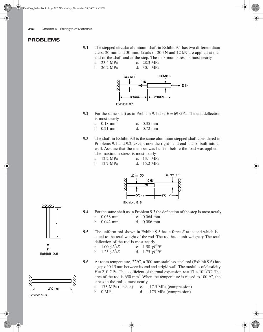
9.1 The stepped circular aluminum shaft in Exhibit 9.1 has two different diam-eters: 20 mm and 30 mm. Loads of 20 kN and 12 kN are applied at the end of the shaft and at the step. The maximum stress is most nearlya. 23.4 MPa c. 28.3 MPab. 26.2 MPa d. 30.1 MPa
9.2 For the same shaft as in Problem 9.1 take E = 69 GPa. The end deflection is most nearlya. 0.18 mm c. 0.35 mmb. 0.21 mm d. 0.72 mm
9.3 The shaft in Exhibit 9.3 is the same aluminum stepped shaft considered in Problems 9.1 and 9.2, except now the right-hand end is also built into a wall. Assume that the member was built in before the load was applied. The maximum stress is most nearlya. 12.2 MPa c. 13.1 MPab. 12.7 MPa d. 15.2 MPa
9.4 For the same shaft as in Problem 9.3 the deflection of the step is most nearlya. 0.038 mm c. 0.064 mmb. 0.042 mm d. 0.086 mm
9.5 The uniform rod shown in Exhibit 9.5 has a force F at its end which is equal to the total weight of the rod. The rod has a unit weight g. The total deflection of the rod is most nearlya. 1.00 g L2/E c. 1.50 g L2/Eb. 1.25 g L2/E d. 1.75 g L2/E
9.6 At room temperature, 22°C, a 300-mm stainless steel rod (Exhibit 9.6) has a gap of 0.15 mm between its end and a rigid wall. The modulus of elasticity E = 210 GPa. The coefficient of thermal expansion a = 17 × 10−6/°C. The area of the rod is 650 mm2. When the temperature is raised to 100 °C, the stress in the rod is most nearlya. 175 MPa (tension) c. −17.5 MPa (compression)b. 0 MPa d. −175 MPa (compression)
Exhibit 9.1
Exhibit 9.3
Exhibit 9.5
Exhibit 9.6
FundEng_Index.book Page 312 Wednesday, November 28, 2007 4:42 PM

Problems 313
9.7 A steel cylindrical pressure vessel is subjected to a pressure of 21 MPa. Its outer diameter is 4.6 m, and its wall thickness is 200 mm. The maximum principal stress in this vessel is most nearlya. 183 MPa c. 362 MPab. 221 MPa d. 432 MPa
9.8 A pressure vessel shown in Exhibit 9.8 is known to have an internal pressure of 1.4 MPa. The outer diameter of the vessel is 300 mm. The vessel is made of steel; v = 0.3 and E = 210 GPa. A strain gage in the circumferential direction on the vessel indicates that, under the given pressure, the strain is 200 × 10−6. The wall thickness of the pressure vessel is most nearlya. 3.2 mm c. 6.4 mmb. 4.3 mm d. 7.8 mm
9.9 An aluminum pressure vessel has an internal pressure of 0.7 MPa. The vessel has an outer diameter of 200 mm and a wall thickness of 3 mm. Poisson’s ratio is 0.33 and the modulus of elasticity is 69 GPa for this material. A strain gage is attached to the outside of the vessel at 45° to the longitudinal axis as shown in Exhibit 9.9. The strain on the gage would read most nearlya. 40 × 10−6 c. 80 × 10−6
b. 60 × 10−6 d. 160 × 10−6
9.10 If sx = −3 MPa, sy = 5 MPa, and txy = −3 MPa, the maximum principal stress is most nearlya. 4 MPa c. 6 MPab. 5 MPa d. 7 MPa
9.11 Given that sx = 5 MPa, sy = −1 MPa, and the maximum principal stress is 7 MPa, the shear stress txy is most nearlya. 1 MPa c. 3 MPab. 2 MPa d. 4 MPa
9.12 Given ex = 800 µ, ey = 200 µ, and gxy = 400 µ, the maximum principal strain is most nearlya. 840 µ c. 900 µb. 860 µ d. 960 µ
Exhibit 9.8
Exhibit 9.9
FundEng_Index.book Page 313 Wednesday, November 28, 2007 4:42 PM

314 Chapter 9 Strength of Materials
9.13 A steel plate in a state of plane stress has the same strains as in Problem 9.12: ex = 800 µ, ey = 200 µ, and gxy = 400 µ. Poisson’s ratio v = 0.3 and the modulus of elasticity E = 210 GPa. The maximum principal stress in the plane is most nearlya. 109 MPa c. 173 MPab. 132 MPa d. 208 MPa
9.14 A stepped steel shaft shown in Exhibit 9.14 has torques of 10 kN • m applied at the end and at the step. The maximum shear stress in the shaft is most nearlya. 760 MPa c. 870 MPab. 810 MPa d. 930 MPa
9.15 The shear modulus for steel is 83 MPa. For the same shaft as in Problem 9.14, the rotation at the end of the shaft is most nearlya. 0.014° c. 1.4°b. 0.14° d. 14°
9.16 The same stepped shaft as in Problems 9.14 and 9.15 is now built into a wall at its right end before the load is applied (Exhibit 9.16). The maximum stress in the shaft is most nearlya. 130 MPa c. 230 MPab. 200 MPa d. 300 MPa
9.17 For the same shaft as in Problem 9.16, the rotation of the step is most nearlya. 0.2° c. 1.8°b. 1.1° d. 2.1°
9.18 A strain gage shown in Exhibit 9.18 is placed on a circular steel shaft which is being twisted with a torque T. The gage is inclined 45° to the axis. If the strain reads e45 = 245 m, the torque is most nearlya. 1000 N•m c. 1570 N•mb. 1230 N•m d. 2635 N•m
Exhibit 9.14
Exhibit 9.16
Exhibit 9.18
FundEng_Index.book Page 314 Wednesday, November 28, 2007 4:42 PM
Problems 315
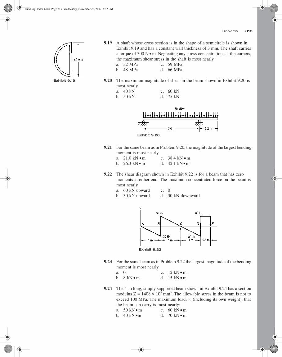
9.19 A shaft whose cross section is in the shape of a semicircle is shown in Exhibit 9.19 and has a constant wall thickness of 3 mm. The shaft carries a torque of 300 N • m. Neglecting any stress concentrations at the corners, the maximum shear stress in the shaft is most nearlya. 32 MPa c. 59 MPab. 48 MPa d. 66 MPa
9.20 The maximum magnitude of shear in the beam shown in Exhibit 9.20 is most nearlya. 40 kN c. 60 kNb. 50 kN d. 75 kN
9.21 For the same beam as in Problem 9.20, the magnitude of the largest bending moment is most nearlya. 21.0 kN • m c. 38.4 kN • mb. 26.3 kN • m d. 42.1 kN • m
9.22 The shear diagram shown in Exhibit 9.22 is for a beam that has zero moments at either end. The maximum concentrated force on the beam is most nearlya. 60 kN upward c. 0b. 30 kN upward d. 30 kN downward
9.23 For the same beam as in Problem 9.22 the largest magnitude of the bending moment is most nearlya. 0 c. 12 kN • mb. 8 kN • m d. 15 kN • m
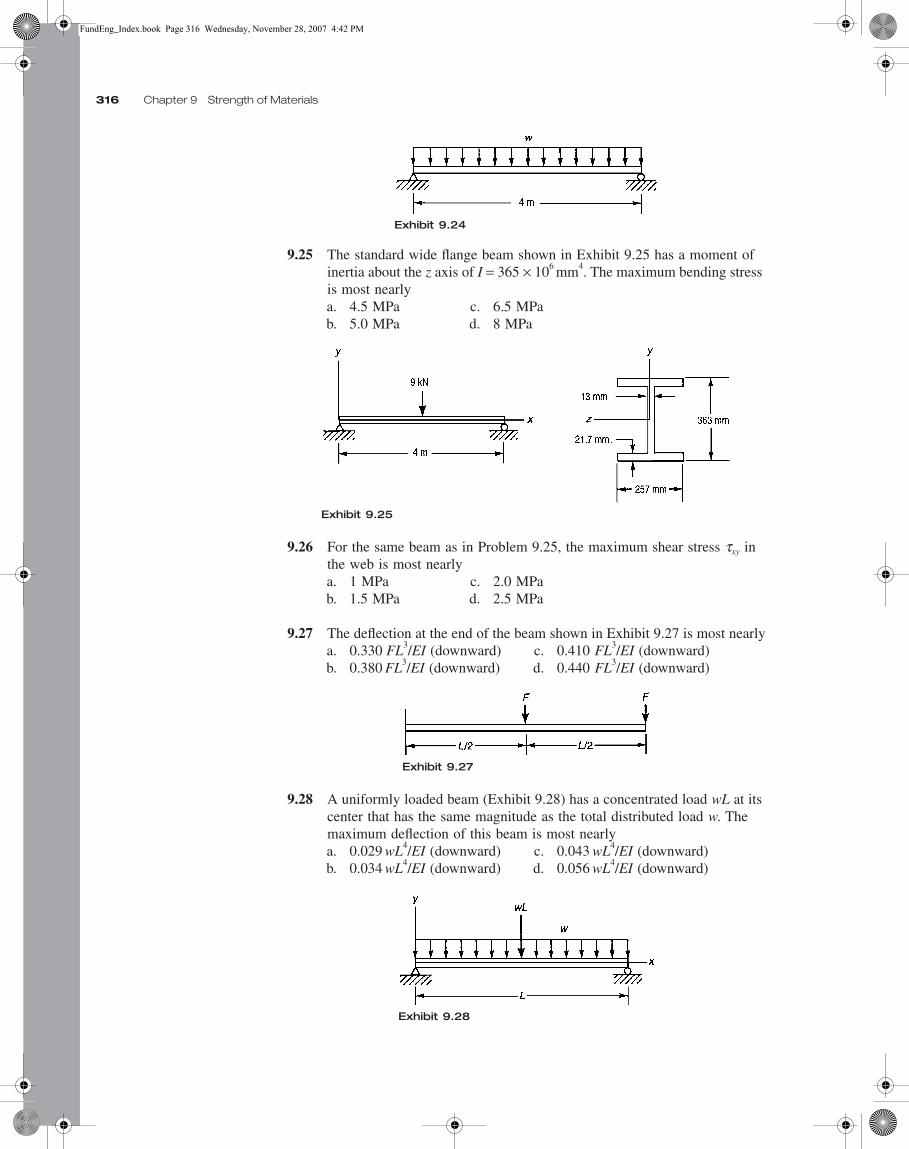
9.24 The 4-m long, simply supported beam shown in Exhibit 9.24 has a section modulus Z = 1408 × 103 mm3. The allowable stress in the beam is not to exceed 100 MPa. The maximum load, w (including its own weight), that the beam can carry is most nearly:a. 50 kN • m c. 60 kN • mb. 40 kN •m d. 70 kN • m
Exhibit 9.20
Exhibit 9.22
Exhibit 9.19
FundEng_Index.book Page 315 Wednesday, November 28, 2007 4:42 PM
316 Chapter 9 Strength of Materials
9.25 The standard wide flange beam shown in Exhibit 9.25 has a moment of inertia about the z axis of I = 365 × 106 mm4. The maximum bending stress is most nearlya. 4.5 MPa c. 6.5 MPab. 5.0 MPa d. 8 MPa
9.26 For the same beam as in Problem 9.25, the maximum shear stress txy in the web is most nearlya. 1 MPa c. 2.0 MPab. 1.5 MPa d. 2.5 MPa
9.27 The deflection at the end of the beam shown in Exhibit 9.27 is most nearlya. 0.330 FL3/EI (downward) c. 0.410 FL3/EI (downward)b. 0.380 FL3/EI (downward) d. 0.440 FL3/EI (downward)
9.28 A uniformly loaded beam (Exhibit 9.28) has a concentrated load wL at its center that has the same magnitude as the total distributed load w. The maximum deflection of this beam is most nearlya. 0.029 wL4/EI (downward) c. 0.043 wL4/EI (downward)b. 0.034 wL4/EI (downward) d. 0.056 wL4/EI (downward)
Exhibit 9.24
Exhibit 9.25
Exhibit 9.27
Exhibit 9.28
FundEng_Index.book Page 316 Wednesday, November 28, 2007 4:42 PM
Problems 317
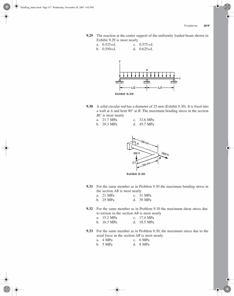
9.29 The reaction at the center support of the uniformly loaded beam shown in Exhibit 9.29 is most nearlya. 0.525wL c. 0.575 wLb. 0.550wL d. 0.625wL
9.30 A solid circular rod has a diameter of 25 mm (Exhibit 9.30). It is fixed into a wall at A and bent 90° at B. The maximum bending stress in the section BC is most nearlya. 21.7 MPa c. 32.6 MPab. 29.3 MPa d. 45.7 MPa
9.31 For the same member as in Problem 9.30 the maximum bending stress in the section AB is most nearlya. 21 MPa c. 31 MPab. 25 MPa d. 39 MPa
9.32 For the same member as in Problem 9.30 the maximum shear stress due to torsion in the section AB is most nearlya. 15.2 MPa c. 17.4 MPab. 16.3 MPa d. 18.5 MPa
9.33 For the same member as in Problem 9.30, the maximum stress due to the axial force in the section AB is most nearlya. 4 MPa c. 6 MPab. 5 MPa d. 8 MPa
Exhibit 9.29
Exhibit 9.30
FundEng_Index.book Page 317 Wednesday, November 28, 2007 4:42 PM

318 Chapter 9 Strength of Materials
9.34 For the same member as in Problem 9.30, the maximum principal stress in the section AB is most nearlya. 17 MPa c. 39 MPab. 27 MPa d. 44 MPa
9.35 A truss is supported so that it can’t move out of the plane (Exhibit 9.35). All members are steel and have a square cross section 25 mm by 25 mm. The modulus of elasticity for steel is 210 GPa. The maximum load P that can be supported without any buckling is most nearlya. 14 kN c. 34 kNb. 25 kN d. 51 kN
9.36 A beam is pinned at both ends (Exhibit 9.36). In the x-y plane it can rotate about the pins, but in the x-z plane the pins constrain the end rotation. In order to have buckling equally likely in each plane, the ratio b/a is most nearlya. 0.5 c. 1.5b. 1.0 d. 2.0
Exhibit 9.35
Exhibit 9.36
FundEng_Index.book Page 318 Wednesday, November 28, 2007 4:42 PM

Solutions 319
SOLUTIONS
9.1 c. Draw free-body diagrams. Equilibrium of the center free-body diagram gives
F1 = 20 − 12 = 8 kN
The areas are
A1 = pr2 = p(10 mm)2 = 314 mm2
A2 = pr2 = p(15 mm)2 = 707 mm2
The stresses are
9.2 b. The force-deformation equations give
Compatibility of deformation gives
9.3 c. Draw the free-body diagrams. From the center free-body diagram, sum-mation of forces yields
F2 = 12 kN + F1
Force-deformation relations are
Compatibility gives
dend = 0 = d1 + d2 = 0.01384 F1 + 0.00410 F2
Exhibit 9.1a
Exhibit 9.3a
σ
σ
1 2
8314
25 5= = =
= = =
PAPA
kNmm
MPa
20 kN707mm
28.3MPa2 2
.
δ
δ
11
2
= = =
= = =
P L
A E
P L
A E
1
1 12
2 2
2 22
(8kN)(300mm)(314 mm )(69GPa)
0.1107mm
(20 kN)(250mm)(707mm )(69GPa)
0.1025mm
δ δ δend mm= + = + =1 2 0 1107 0 1025 0 213. . .
δ
δ
11 1
1 1
22 2
2 2
22707
0 00410
= = =
= = =
P L
A E
FF
P L
A E
FF
( kN)(300mm)
(314mm )(69GPa)0.01384
kN)(200mm)
mm )(69GPa
12 1
2
(
( ).
FundEng_Index.book Page 319 Wednesday, November 28, 2007 4:42 PM

320 Chapter 9 Strength of Materials
Substitution of the equilibrium relation, F2 = 12 + F1, into the above equation gives
0 = 0.01384 F1 + 0.00410 (12 + F1)F1 = −2.74 kN, F2 = 9.26 kN
The stresses are
9.4 a. The same three-step process as in Problem 9.3 must be carried out. Since this process has already been completed, the results can be used. The deflection can be expressed as
d = d1 = −d2 = 0.01384 F1 = 0.01384 (−2.74) = −0.0380 mm
9.5 c. Draw a free-body diagram. Summation of forces in the vertical direction gives
9.6 d. A force will develop in the rod if it attempts to grow more than 0.15 mm. Assuming that it does grow that amount, the displacement is
9.7 b. In a cylindrical pressure vessel the three principal stresses are
The maximum is σt, which gives
9.8 b. The stresses in the pressure vessel are, as in the last problem,
The wall thickness is usually thin enough so that it can be assumed that
σ σ1 2
2 74314
8 739 26
13 10= = − = − = = =P
A
P
A
( . )( )
.( . )
.kN
mmMPa;
kN(707mm )
MPa2 2
Exhibit 9.5a
P AL Ax
PAE
dxA L x
AEdx
EL
L LE
L L
= +
= = + = +
=∫ ∫γ γ
δ γ γ γ0 0
22 2
232
( )
δ α
σ
= + − =
= + ×°
° − °
= += −
= = − = −
−
PLAE
L t t
P
PP
PA
o( ) .
( )( )( )
.
..
0 15
617 10
1300 100
0 15
112 7650
173 5
6
2
mm
(300mm)50mm)(210GPa C
mm C 22 C
mm 0.00220 0.3978112.7 kN
kNmm
MPa
σ σ σt a rqD t qD t= = ≈/ ; / ;2 4 0
σ t
qD
t= = − =
2(21MPa)(4600 mm 400 mm)
2(200 mm)221MPa
σ σ σt a r
qDt
qDt
= = ≈2 4
0; ;
D Di o≈
FundEng_Index.book Page 320 Wednesday, November 28, 2007 4:42 PM
Solutions 321
The tangential strain can be found from Hooke’s law:
The thickness is then
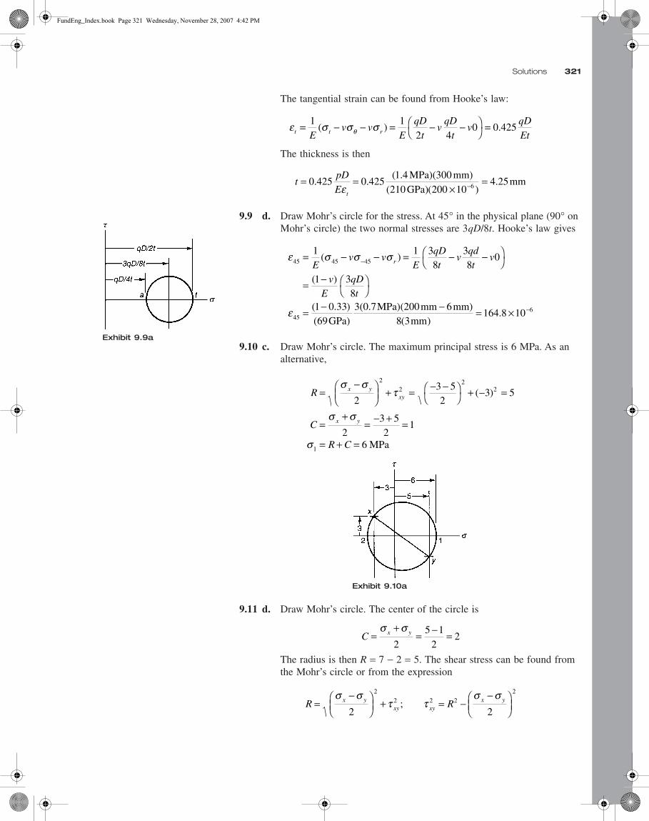
9.9 d. Draw Mohr’s circle for the stress. At 45° in the physical plane (90° on Mohr’s circle) the two normal stresses are 3qD/8t. Hooke’s law gives
9.10 c. Draw Mohr’s circle. The maximum principal stress is 6 MPa. As an alternative,
9.11 d. Draw Mohr’s circle. The center of the circle is
The radius is then R = 7 − 2 = 5. The shear stress can be found from the Mohr’s circle or from the expression
Exhibit 9.10a
ε σ σ σθt t rEv v
E
qD
tv
qD
tv
qD
Et= − − = − −
=1 1
2 40 0 425( ) .
tpD
E t
= =×
=−0 425 0 4251 4
210 200 104 256. .
( .( ( )
.ε
MPa)(300 mm)GPa)
mm
Exhibit 9.9a
ε σ σ σ
ε
45 45 45
456
1 1 38
38
0
1 38
1 0 3369 8 3
164 8 10
= − − = − −
= −
= − − = ×
−
−
Ev v
EqDt
vqdt
v
vE
qDt
r( )
( )
( . )( ( )
.GPa)
3(0.7MPa)(200mm 6mm)mm
R
C
R C
x yxy
x y
=−
+ = − −
+ − =
=+
= − + =
= + =
σ στ
σ σ
σ
23 52
3 5
23 52
1
6
2
22
2
1
( )
MPa
C x y=+
= − =σ σ
25 1
22
R Rx yxy xy
x y=−
+ = −−
σ στ τ
σ σ2 2
2
2 2 2
2
;
FundEng_Index.book Page 321 Wednesday, November 28, 2007 4:42 PM
322 Chapter 9 Strength of Materials
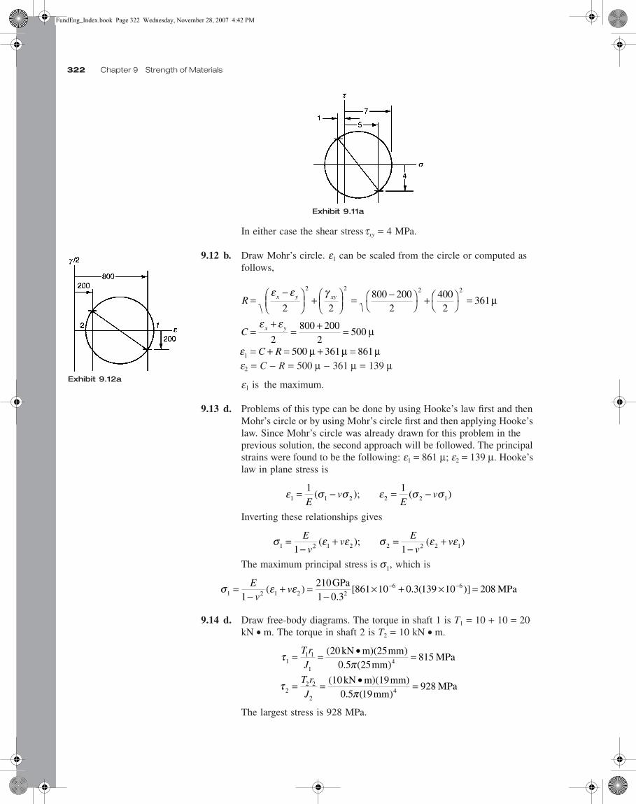
In either case the shear stress txy = 4 MPa.
9.12 b. Draw Mohr’s circle. e1 can be scaled from the circle or computed as follows,
e2 = C − R = 500 µ − 361 µ = 139 µ
e1 is the maximum.
9.13 d. Problems of this type can be done by using Hooke’s law first and then Mohr’s circle or by using Mohr’s circle first and then applying Hooke’s law. Since Mohr’s circle was already drawn for this problem in the previous solution, the second approach will be followed. The principal strains were found to be the following: e1 = 861 µ; e2 = 139 µ. Hooke’s law in plane stress is
Inverting these relationships gives
The maximum principal stress is , which is
9.14 d. Draw free-body diagrams. The torque in shaft 1 is T1 = 10 + 10 = 20 kN • m. The torque in shaft 2 is T2 = 10 kN • m.
The largest stress is 928 MPa.
Exhibit 9.11a
R
C
C R
x y xy
x y
=−
+
= −
+
=
=+
= + =
= + = + =
ε ε γ
ε ε
ε
2 2800 200
24002
361
2800 200
2500
500 361 861
2 2 2 2
1
µ
µ
µ µ µ
Exhibit 9.12a
ε σ σ ε σ σ1 1 2 2 2 1
1 1= − = −E
vE
v( ); ( )
σ ε ε σ ε ε1 2 1 2 2 2 2 11 1=
−+ =
−+E
vv
Ev
v( ); ( )
σ1
σ ε ε1 2 1 2 26 6
12101 0 3
861 10 0 3 139 10 208=−
+ =−
× + × =− −Ev
v( ).
[ . ( )]GPa
MPa
τπ
τπ
11 1
14
2 2
24
200 5 25
815
0 5 19928
= = • =
= = • =
T r
J
T r
J
( ). ( )
. ( )
kN m)(25mmmm
MPa
(10 kN m)(19mm)mm
MPa2
FundEng_Index.book Page 322 Wednesday, November 28, 2007 4:42 PM

Solutions 323
9.15 d. From the force-deformation relations,
From compatibility,
f = f1 + f2 = 5.63° + 8.43° = 14.06°
9.16 d. Draw the free-body diagrams. Equilibrium of the center free body gives
T1 = T2 + 10
The force-deformation relations are
Compatibility requires that
f1 + f2 = 0 = 49.1 × 10⁻³ + (4.91 × 10⁻³ + 14.7 × 10⁻³)T2
Solving for the torques gives
The stresses then are
Exhibit 9.14a
φπ
φπ
11 1
14
22 2
24
83 0 5 250 982 5 63
83 0 5 190 1471 8 43
= = • = = °
= = • = = °
T L
GJ
T L
GJ
(( ) . (
. .
(( ) . (
. .
20 kN m)(250mm)GPa mm)
rad
10 kN m)(250mm)GPa mm)
rad
Exhibit 9.16a
φπ
φπ
11 1
1
24
3 32
22 2
2
24
32
10 250
83 0 5 2549 1 10 4 91 10
250
83 0 5 1914 7 10
= =+
= × + ×
= = = ×
− −
−
T L
GJ
TT
T r
J
TT
( )( )
( ) . ( ). .
(
( ) . ( ).
mm
GPa mm
mm)
GPa mm
T
T T
2
2
5 3052 207
2 50
10 2 50 10 7 50
= = − •
= + = − + = •
.
..
. .
kN m
kN m1
τπ
τπ
11 1
14
2 2
24
7 500 5 25
306
2 50 5 19
232
= = • =
= = − • = −
T r
J
T r
J
( . ). (
( . ). (
kN m)(25mmmm)
MPa
kN m)(19mmmm)
MPa2
FundEng_Index.book Page 323 Wednesday, November 28, 2007 4:42 PM

324 Chapter 9 Strength of Materials
9.17 d. The same three-step process as in Problem 9.16 must be carried out. Since this process has already been completed, the results can be used. The rotation can be expressed as
9.18 a. For a torsion problem, the shear strain is
Other shear strains in the r − f orientation are zero. Mohr’s circle for this state of strain is shown in Exhibit 9.18(a). From Mohr’s circle,
9.19 d. In thin-walled shafts the shear stress is
The area A is the cross-sectional area of the shaft including the hole so,
9.20 c. Draw the free-body diagram of the beam, replacing the distributed load with its statically equivalent loads. Summation of moments about the left end gives
0 = −3.6 R2 + (108)(1.8) + (36)(4.2)R2 = 96 kN
Summation of forces in the vertical direction gives
R1 = 144 − 96 = 48 kN
Exhibit 9.18a
φ φ φπ
= = − = = • = = °1 21 1
1
7 5083
0 0368 2 11T L
GJ( .(
. .kN m)(250mm)
GPa)0.5 (25mm)rad4
γτ
φφ
zz
G
Tr
GJ= =
εγ τ
ε π
φ φ45
454 6
2 2 22 2 83 0 5 25 245 10
25998
= = =
= = × = •−
z z
GTrGJ
TGJ
r( )[ . ( ]( )GPa mm)
mmN m
τ sz
T
At=
2
Ar
TAtsz
= = − =
= = • =
π π
τ
2 22
225
2760
2
( )mm 3mmmm
300N m2(760mm )(3mm)
65.7 MPa2
FundEng_Index.book Page 324 Wednesday, November 28, 2007 4:42 PM

Solutions 325
This is enough information to plot the shear diagram (Exhibit 9.20b). The largest magnitude of shear is 60 kN.
9.21 c. The maximum bending moment occurs where the shear is zero. From the shear diagram, the distance to the zero from the left end can be found by similar triangles.
The areas of the shear diagrams are the changes in moment (Exhibit 9.21a).
Exhibit 9.20a
Exhibit 9.20b
Exhibit 9.21a
Exhibit 9.21b
48 1083 6
48 3 6108
1 6x
x= = =.
;( )( . )
. m
A
A
1
2
= = •
= = •
(48kN)(1.6m)2
38.4 kN m
(36kN)(1.2m)2
21.6kN m
FundEng_Index.book Page 325 Wednesday, November 28, 2007 4:42 PM
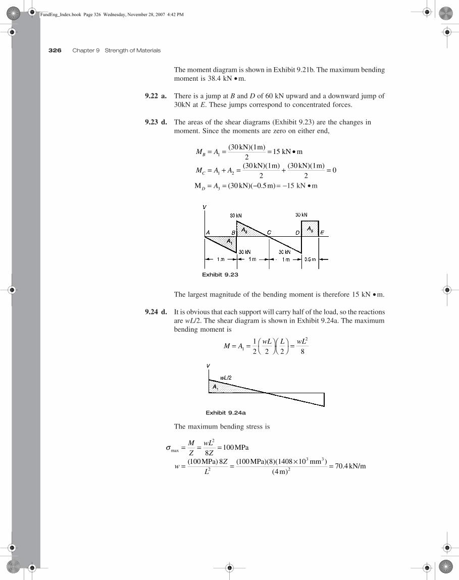
326 Chapter 9 Strength of Materials
The moment diagram is shown in Exhibit 9.21b. The maximum bending moment is 38.4 kN • m.
9.22 a. There is a jump at B and D of 60 kN upward and a downward jump of 30kN at E. These jumps correspond to concentrated forces.
9.23 d. The areas of the shear diagrams (Exhibit 9.23) are the changes in moment. Since the moments are zero on either end,
= −15 kN • m
The largest magnitude of the bending moment is therefore 15 kN • m.
9.24 d. It is obvious that each support will carry half of the load, so the reactions are wL/2. The shear diagram is shown in Exhibit 9.24a. The maximum bending moment is
The maximum bending stress is
Exhibit 9.23
Exhibit 9.24a
M A
M A A
B
C
= = = •
= + = + =
1
1 2
(30 kN)(1m)2
15 kN m
(30 kN)(1m)2
(30 kN)(1m)2
0
M 30 kN)( 0.5m)D A= = −3 (
M AwL L wL= =
=1
212 2 2 8
σ max
( ( )( )
.
= = =
= = × =
MZ
wLZ
wZ
L
2
2 2
8100
100 8 1004
70 4
MPa
MPa) MPa)(8)(1408 10 mmm
kN/m3 3
FundEng_Index.book Page 326 Wednesday, November 28, 2007 4:42 PM

Solutions 327
9.25 a. Draw the free-body diagram and the shear and moment diagrams as shown in Exhibit 9.25a. The maximum bending stress is
9.26 a. From the previous problem, the maximum shear in the beam is 4.5 kN. The maximum shearing stress will take place at the centroid (Exhibit 9.26), so a cut must be made there in order to calculate Q. The moment of the area Q is, therefore,
The maximum shear stress is then
Exhibit 9.25a
Exhibit 9.26
σ maxmax
(
).= =
• ( )×
=M c
I
94 48
363
4
kN m)
(365 10 mmMPa
mm
26
Q A y A y
Q
Q
= +
= −
+ + −
×−
= ×
1 1 2 2
6 3
257
1 117 10
(
.
mm)(21.7mm)363mm
221.7mm
2363mm
221.7mm
(13mm)21.7mm
2
mm
363 mm
2
�
τ = = ××
=VQ
Ib
(4.5kN)(1.117 10 mm )(365 10 mm )(13mm)
1.060 MPa6 3
6 4
FundEng_Index.book Page 327 Wednesday, November 28, 2007 4:42 PM
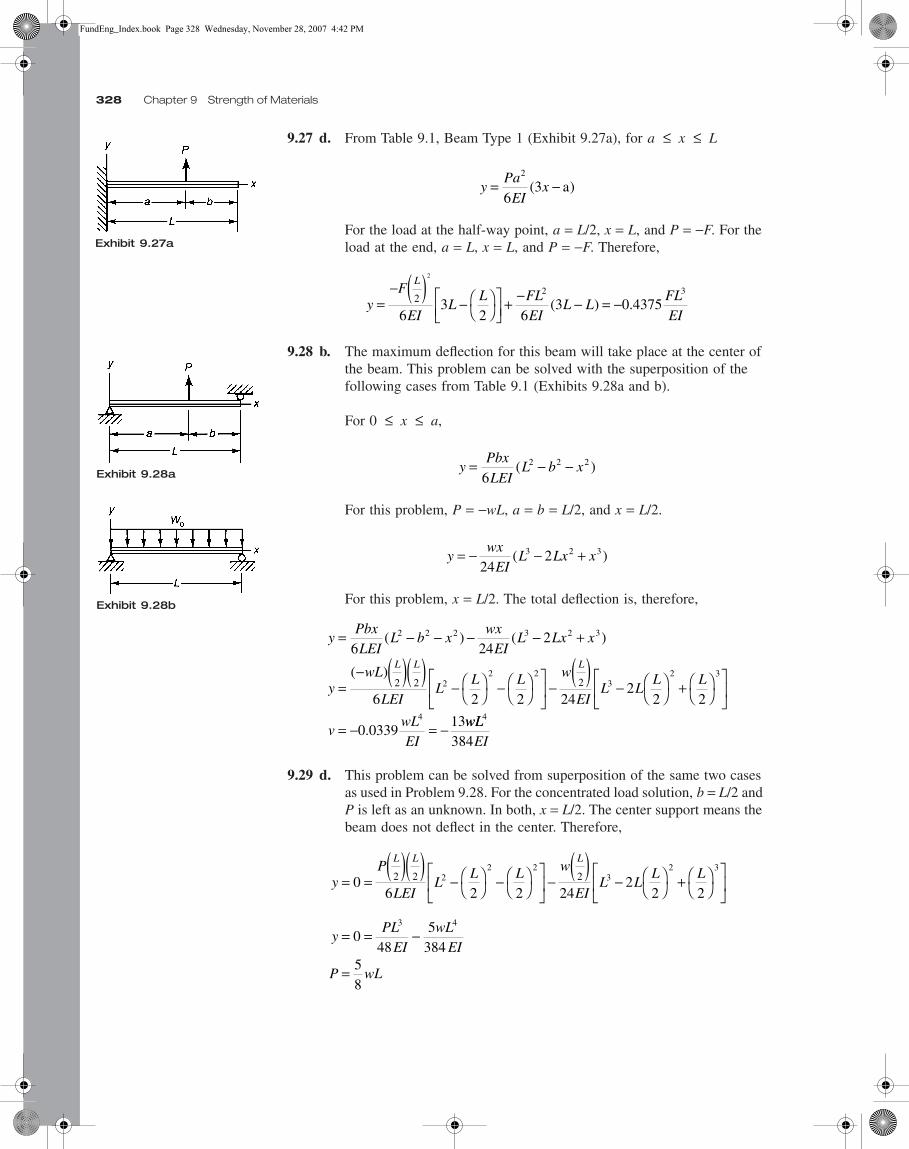
328 Chapter 9 Strength of Materials
9.27 d. From Table 9.1, Beam Type 1 (Exhibit 9.27a), for a x L
For the load at the half-way point, a = L/2, x = L, and P = −F. For the load at the end, a = L, x = L, and P = −F. Therefore,
9.28 b. The maximum deflection for this beam will take place at the center of the beam. This problem can be solved with the superposition of the following cases from Table 9.1 (Exhibits 9.28a and b).
For 0 x a,
For this problem, P = −wL, a = b = L/2, and x = L/2.
For this problem, x = L/2. The total deflection is, therefore,
9.29 d. This problem can be solved from superposition of the same two cases as used in Problem 9.28. For the concentrated load solution, b = L/2 and P is left as an unknown. In both, x = L/2. The center support means the beam does not deflect in the center. Therefore,
Exhibit 9.27a
≤ ≤
yPa
EIx= −
2
63( )a
yF
EIL
L FLEI
L LFLEI
L
=− ( )
−
+ − − = −2
2
63
2 63 0 4375
2 3
( ) .
≤ ≤
yPbx
LEIL b x= − −
62 2 2( )Exhibit 9.28a
Exhibit 9.28b
ywx
EIL Lx x= − − +
2423 2( )3
yPbxLEI
L b xwx
EIL Lx x
ywL
LEIL
L L w
EIL L
L L
vwLEI
L L L
= − − − − +
=− ( )( )
−
−
−
( )−
+
= − = −
6 242
6 2 2 242
2 2
0 033913
2 2 2 3 2 3
22 2
32 3
4
2 2 2
( ) ( )
( )
.wLwL
EI
4
384
yP
LEIL
L L w
EIL L
L L
yPL
EIwL
EI
P wL
L L L
= =( )( )
−
−
−
( )−
+
= = −
=
06 2 2 24
22 2
048
5384
58
2 2 222 2
32 3
3 4
FundEng_Index.book Page 328 Wednesday, November 28, 2007 4:42 PM

Solutions 329
9.30 c. Draw the free-body diagram (Exhibit 9.30a). From a summation of moments about the cut at B, the maximum bending moment in BC is the moment M = 200 N × 250 mm or 50 kN • m. The maximum bending stress is
9.31 d. Draw the free-body diagram (Exhibit 9.31). The maximum stresses in section AB will occur at A. Summation of forces in the vertical direction gives VA = 200 N. Summation of forces along the direction of the rod AB gives P = 2000 N. Summation of moments along the rod AB gives TA = 200 N × 250 mm or 50 kN • mm. Summation of moments at the cut perpendicular to the rod AB gives MA = 200 N × 300 mm = 600 kN • mm. The maximum bending stress is
9.32 b. From the free-body diagram in Problem 9.31, the maximum torque is 50 kN • mm. The maximum shear stress is, therefore,
9.33 a. From the free-body diagram in Problem 9.31, the maximum axial force is 2000 N. The maximum stress due to this force is, therefore,
Exhibit 9.30a
Exhibit 9.31
σπ
= = • =McI
(. ( . )
500 25 12 5 4
kN mm)(12.5mm)mm
32.6 MPa
σπ
= = • =McI
(. (
60 kN mm)(12.5mm).5mm)
39.1 MPa40 25 12
τπmax
max (. ( .
= = • =T r
J0 5
0 5 12 50 kN mm)(12.5mm)
mm)16.30 MPa4
σπ
= = =P
A
200012 5
4 072
Nmm
MPa( . )
.
FundEng_Index.book Page 329 Wednesday, November 28, 2007 4:42 PM

330 Chapter 9 Strength of Materials
9.34 d. The stresses were found in the previous three problems. There is an axial stress due to both bending and axial loads. This stress is
s = 39.1 MPa + 4.07 MPa = 43.2 MPa
The shear stress is 16.3 MPa. These are the only non-zero stresses. The maximum principal stress can be calculated as follows,
9.35 a. Draw the free-body diagram of the joint B (Exhibit 9.35a). Summation of forces in the vertical direction gives
Summation of forces in the horizontal direction gives
Solving for FAB and FBC gives
The member AC is in tension and does not need to be considered. The moment of inertia for both members is
The critical buckling load for member AB is
The load P for buckling to occur in AB is
The critical buckling load for member BC is
R
C
C R
x yxy
x y
=−
+ = −
+ =
=+
= + =
= + = + =
σ στ
σ σ
σ
243 2 0
216 3 22 0
243 2 0
221 6
22 0 21 6 43 6
2
22
2
1
.. .
..
. . .
MPa
MPa
MPa
Exhibit 9.35a
P F FAB BC=+
++
1 5
1 5 0 9
1 5
2 7 1 52 2 2 2
.
. .
.
. .
F FAB BC
0 9
1 5 0 9
2 7
2 7 1 52 2 2 2
.
. .
.
. .+=
+
F P F PAB BC= =0 875 0 515. ; .
Ibh= = =
34
1225
1232 600
(,
mm)(25mm)mm
3
P FEI
LABcr
2 4
2 2
(210GPa)(32,600 )(1.5m) (0.9m)
22.0 kN= = =+
=π π2
2
P = =22 kN0.875
25.2 kN
P FEI
LBCcr
2 4
2 2
(210GPa)(32,600mm )[(2.7m) (1.5m) ]
7.07 kN= = =+
=π π2
2
FundEng_Index.book Page 330 Wednesday, November 28, 2007 4:42 PM
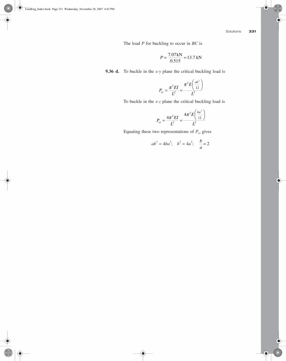
Solutions 331
The load P for buckling to occur in BC is
9.36 d. To buckle in the x-y plane the critical buckling load is
To buckle in the x-z plane the critical buckling load is
Equating these two representations of Pcr gives
ab3 = 4ba3; b2 = 4a2;
P = =7.07kN0.515
3.7 kN1
PEI
L
E
L
ab
cr = =
π π2
2
2
2
3
12
PEI
L
E
L
ba
cr = =
4
42
2
2
2
3
12π π
b
a= 2
FundEng_Index.book Page 331 Wednesday, November 28, 2007 4:42 PM

FundEng_Index.book Page 332 Wednesday, November 28, 2007 4:42 PM