road pavement construction and maintenance using … · basic tools for such predictions for...
TRANSCRIPT
BTE Publicat ion Summary
Date
Search
Results
Subject
Series
A to Z
Exit
GO BACK
Pavement Management: Development of a Life Cycle Costing Technique
Occasional PaperThis paper provides a simple method for evaluating alternative strategies for road pavement construction and maintenance using a life cycle costing approach.
Bureau of Transport and Communications Economics
Pavement Management : Development of a Life Cycle
Costing Technique
AUSTRALIAN GOVERNMENT PUBLISHING SERVICE, CANBERRA
0 Commonwealth of Australia 1990
ISBN 0 644 10287 X ISSN 1032-0539
This work is copyright. Apart from any use as permitted under the Copyright Act 1968, no part may be reproduced by any process without written permission from the Director Publishing and Marketing, AGPS. Inquiries should be directed to the Manager, AGPS Press, Australian Government Publishing Service, GPO Box 84, Canberra, ACT 2601.
Printed in Australia by Better Printing Service, 1 Foster Street, Queanbeyan N.S.W. 2620
FOREWORD
This paper provides a method for evaluating strategies for road pavement construction and maintenance. It outlines a comparison of road pavement deterioration algorithms, presents a simple model for the analysis of flexible road pavements in Australia, and discusses that models application.
Engineering skills are improving to the point that predictions can now be made of the likely condition of road pavements throughout their life. This study provides basic tools for such predictions for flexible pavements under a range of environmental, maintenance and operational conditions.
The life cycle costing model detailed in this paper is a powerful technique that can be used to analyse the interactions of the road pavement, traffic and environmental conditions over time and to develop a more comprehensive understanding of road pavement deterioration and rehabilitation.
This work and the subsequent use of the resulting computer analysis will enhance research capabilities in examining road cost recovery issues.
The research forthis paperwas undertaken by Messrs J:E. Millerand K. Y. Loong with the assistance of Kinhill Engineers Pty Ltd and Dynatest PMS.
Anthony Ockwell Research Manager
Bureau of Transport and Communications Economics Canberra July 1990
iii
CONTENTS
FOREWORD
ABSTRACT
SUMMARY
CHAPTER 1
CHAPTER 2
CHAPTER 3
CHAPTER 4
CHAPTER 5
INTRODUCTION
CONCEPTS BEHIND THE DEVELOPMENT OF AN ANALYTICAL TECHNIQUE Concept of life cycle costing Some fundamental considerations Computer programs available for road analysis Development of a life cycle costing technique
PAVEMENT DETERIORATION.RELATl0NSHlPS Assessing the algorithms The algorithm and Australian conditions
DESCRIPTION OF THE LIFE CYCLE COSTING COMPUTER MODEL Road length and traffic modules Existing and proposed pavement condition modules Intervention points module Impact of intervention module Local calibration factors module Construction and maintenance costs module Vehicle operating costs module Net present value module
OUTPUTS AND APPLICATION OF THE LIFE CYCLE COSTING MODEL Use of the model for pavement life assessment Maintenance, reseal and asphalt overlay options Further applications and limitations of the model
Page iii
xi
xiii
1
1 1 12 18
21 24 24 29 31 32 32 33 34
35 35 36 40
V
CHAPTER 6 CONCLUSIONS Page 43
APPENDIX I DEFLECTIONS AND STRUCTURAL NUMBERS FOR NEW PAVEMENTS 45
51
57
61
APPENDIX II CONSTRUCTION AND MAINTENANCE COSTS
REFERENCES
ABBREVIATIONS
vi
TABLES
4.1
4.2
4.3
4.4
5.1
5.2
5.3
5.4
I. 1
1.2
1.3
1.4
1.5
1.6
Possible intervention based on IRI roughness criteria
Possible intervention based on NAASRA roughness criteria
Possible time-based maintenance triggers
Recommended values for the environmental coefficient m for various climates
Life cycle costing analysis of possible terminal roughness options for a low traffic road
Life cycle costing analysis of possible terminal roughness options for a high traffic divided road
Life cycle costing analysis of reseal options
Life cycle costing analysis of asphalt overlay options
Thin bituminous surfacing: pavement thickness requirements
Thin bituminous surfacing, 500 megapascal basecourse: deflections
Thin bituminous surfacing, 500 megapascal basecourse: structural numbers
Thin bituminous surfacing, 350 megapascal basecourse: deflections
Thin bituminous surfacing, 350 megapascal basecourse: structural numbers
Thin bituminous surfacing, 250 megapascal basecourse: deflections
Page 30
30
30
33
36
38
39
40
46
46
47
47
48
48
vi i
Page
structural numbers 49 1.7 Thin bituminous surfacing, 250 megapascal basecourse:
11.1 Construction costs for cross-section A, in 1988 prices 53
11.2 Construction costs for cross-section B, in 1,988 prices 54
11.3 Construction costs for cross-section C, in 1988 prices 55
11.4 Resealing and shape correction costs, in 1988 prices 56
viii
FIGURES
2.1
3.1
4.1
4.2
4.3
4.4
4.5
4.6
5.1
5.2
5.3
11.1
A possible pavement construction and preservation sequence
Progression of various components of roughness
Representative pavement cross-sections used
The life cycle costing model
IRI, NRM and PSI roughness comparison
Relationship of structural number to deflection
Structural number versus design traffic
Improvement in structural number following an asphalt or granular overlay
Life cycle costing analysis of three reconstruction options for a low traffic road
Life cycle costing analysis of three reseal options
Life cycle costing analysis of three asphalt overlay options
Routine maintenance costs
Page 9
13
22
25
27
27
28
32
37
37
41
51
ix
ABSTRACT
This paper presents a method for assessing road pavements using a life cycle costing approach. It discusses the use of the method and outlines the way in which the algorithms were developed.
The project draws on the results of extensive research carried out by the World Bank. It provides a first step towards transforming that work so as to take into account Australian road conditions and pavement measurement characteristics. The paper also includes a discussion of the integration of vehicle operating costs and benefit-cost ratios and of the packaging of this work into a simple spreadsheet computer model.
The model has a number of applications, including the optimisation of construction, maintenance and vehicle operating costs. It can also be used to examine heavy vehicle pavement damage and cost recovery issues. Further, it can be easily calibrated to suit different geographical or environmental conditions and could be extended to the analysis of rigid pavements.
One of the strengths of the model is its flexibility, which will enable it to be restructured to suit particular needs.
xi
SUMMARY
This paper provides a simple method for evaluating alternative strategies for road pavement construction and maintenance using a life cycle costing approach.
It examines a number of pavement deterioration algorithms and discusses the development of a life cycle costing computer model. The most recent World Bank (or Paterson) algorithm was selected as a base for the work. This algorithm was formulated after extensive development work and appeared to be the most suitable for Australian conditions.
Using the algorithm as a starting point, the Bureau developed a road pavement deterioration and life cycle costing analysis tool by incorporating Australian road pavement characteristics covering a wide range of traffic, environmental and maintenance conditions.
The Bureau developed a spreadsheet-based computer model to calculate life cycle costs for flexible pavements. The model can be used to assess the cost and pavement roughness implications of differing pavement types and maintenance and construction strategies with differing traffic levels. It uses the net present value method to assess future costs. Additionally, the model includes a preliminary means of evaluating vehicle operating costs. Using the model, pavement maintenance options can be assessed against the minimisation of total road user costs plus road authority costs or the maximisation of benefits at differing budget levels.
The model was developed primarily forthe examination of single lengths of road, but it can also be integrated with pavement management systems to examine multiple road lengths.
xiii
CHAPTER 1 INTRODUCTION
A primary concern of administrators of the Australian road system has moved from the construction of new roads to the management of existing road infrastructure. For this reason there is a growing need for pavement management systems and analytical tools to evaluate pavements, including pavement use and the resulting deterioration. The life cycle costing model, detailed in this paper, is such an analytical tool.
Life cycle costing can be defined as an economic assessment of road infrastructure and its use during its life. The concept of the ‘life’ of a road pavement is discussed in chapter 2. The total life cycle could include research, planning, design, acquisition, construction, maintenance, operation, disposal, and other costs associated with owning or using such a facility.
This paper presents the results of a study that had as its major objective the development of a methodology for assessing the life cycle costs of road pavements under differing traffic loads and environmental conditions. The study required the development of a road condition measure, and the compilation of capital and maintenance cost data, which could be applied using economic theory ~
to typical road pavements to show how design, construction and maintenance programs might be modified to reduce total life cycle costs.
The Federal Government recognises the importance of ensuring that road construction and maintenance outlays are managed in a cost-efficient manner. The optimum allocation must involve a trade-off between construction, maintenance and vehicle operating costs. The emphasis of most State, Territory and local government authorities is on maintenance and rehabilitation of the existing system rather than on the construction of new roads. Of the $4000 million per annum spent on Australian roads by all levels of government, at least $1 400 million per annum is spent on routine maintenance activities (BTCE 1989). The proportion of total road funds allocated to maintenance is increasing. Because activities such as resealing, overlays and reconstruction are considered as components of the maintenance of a roadway, in this paper the total costs involved are considerable.
The Federal Government’s Australian Centennial Roads Development Program introduces the need for road authorities to adopt pavement management systems to assist in the effective maintenance of the Australian road system.
1
BTCE Occasional Paper 700
In the 1990s road maintenance is expected to assume greater prominence. The use of analytical tools such as the life cycle costing model will provide guidance in formulating future road construction and maintenance strategies.
In developing the life cycle costing methodology and the subsequent computer model, the Bureau took the following steps:
- It determined maintenance 'triggers'. It obtained and organised unit cost data. It selected standard pavement cross-sections. It tested the concepts using data sets. It produced a spreadsheet life cycle costing model.
As the study progressed two workshops were conducted, at which BTCE staff, consultants and road engineers reviewed progress. Following the first workshop and the production of an'interim report, the study proceeded with the collection and compilation of sample cost data and the application of those data to the deterioration algorithm to verify the relationships for traffic levels and road conditions. Typical tabulations were produced following some adjustment of the earlier relationships. Maintenance triggers were then applied to test the impact of roadworks such as maintenance, resealing, and resheetings or overlays. At the conclusion of this stage the second workshop was held; it was attended by local government engineers as well as staff of the Bureau and the Department of Transport and Communications.
To ensure that the study was kept to manageable proportions, the Bureau limited its initial work to sealed roads with flexible pavements. A preliminary model was then developed. This work could be enlarged to cover other pavement types, including rigid pavements and unsealed roads. The research work will provide a basis for expansion by those interested in other pavement issues (such as the impact of traffic and environmental conditions) and for further development of the use of vehicle operating costs as part of the assessment.
It assessed and selected deterioration algorithms.
2

CHAPTER 2 CONCEPTS BEHIND THE DEVELOPMENT OF AN ANALYTICAL TECHNIQUE
This chapter discusses the concept and application of life cycle costing (LCC) to road pavement evaluation, considers currently available road assessment computer models, and discusses the development of the LCC model.
CONCEPT OF LIFE CYCLE COSTING
Life cycle costing is not a new concept. Businesses, industries, government agencies and individuals have been using LCC analysis as a tool for project management and evaluation for many years.
Life cycle costing analysis is often associated with the evaluation of an asset with a definite life expectancy. With periodic upgradings a road pavement may have an indefinite life, but the use of LCC analysis is equally appropriate. This is largely because changes in conditions over the long term do not have a significant impact on the short term results.
Life cycle costing is a means of analysing the total cost of acquisition, construction, operation and maintenance of a product or system during its entire life. LCC analysis introduces the economic theory necessary for the comparison of various systems or equipment for design, support and maintenance alternatives, and it allows for the assessment of risk in the decision-making process. LCC analysis serves to:
define areas with high maintenance and operational costs as aconsequence of design decisions; and provide budget estimates for inclusion in long range cost projection and financial planning data.
More specifically, pavement LCC analysis can assist in comparing rigid and flexible pavements, and in assessing heavy vehicle damage and cost recovery. It can also be used to assess benefits of alternative maintenance strategies.
In general, the following are the major cost categories in LCC analysis:
- production and construction costs; research and development costs;
3
BTCE Occasional Paper 100
maintenance, operating and logistics support costs; and retirement and disposal costs.
The costs associated with research and development and production and construction can normally be grouped into one category - the initial capital cost of the system. The projected or future costs can include the costs of logistics support, maintenance and operating costs and the retirement and disposal costs.
In summary, LCC analysis can be defined as a systematic analytical process of evaluating various alternative courses 0f:action with the objective of selecting the most appropriate way to employ resources (Blanchard 1978, 1986). It is an iterative process devised to achieve a cost-effective solution.
SOME FUNDAMENTAL CONSIDERATIONS
A number of items are pertinent to the selection of a method for analysing competing alternatives on the basis of projected LCC; these items are discussed in the following paragraphs.
The economic life of a road pavement
As noted, in performing life cycle costing analysis one may assume a time span differing from the actual physical life cycle of an item. This time span, identified as the ‘economic life’, is the time that is considered directly relevant to the objective of the analysis and is feasible in terms of acquiring sufficient economic data for decision-making purposes.
In the assessment of life cycle costs it is necessary to examine the construction and subsequent maintenance works on the pavement. The time span should cover the pavement life and would ensure that discounting effects would minimise any residual costs. There is no point in extending the evaluation period excessively as it is difficult to estimate future traffic and deterioration.
Once determined, the analysis period for a particular project should be the same for all design options. In practice, however, the choice of the length of analysis period depends on pavement type, data availability and the designer‘s judgment. The choice of varying analysis periods for different design strategies in an LCC model provides the flexibility for users to satisfy their local requirements.
Net present value method
The net present value method is used for the life cycle costing analysis. All future costs for each year in the life cycle are discounted to the present value. That is, the present value of costs for a given alternative can be calculated by discounting cost elements (such as the initial capital cost of construction, routine maintenance costs, rehabilitation costs, and vehicle operating costs) using adiscount rate. The alternatives can then be evaluated to arrive at an optimal solution.
4
Chapter 2
Choice of discount rate
In project appraisal, a dollar's worth of costs or benefits incurred today should not be treated as having the same effect on the return from the project as a dollar's worth at a distant time. It is therefore important to take account of different time profiles of costs and benefits when assessing public (or private) sector investment proposals. By applying a discount rate, future costs and benefits can be converted into their equivalent values today to obtain the 'present value'.
There is no consensus among economists and planners on the correct choice of a discount rate. In recent years, benefitxost analysis practitioners have devoted much effort to the search for a single discount rate appropriate for public expenditure decisions. Four main approaches have been suggested: - the social rate of time preference (SRTP); m the social opportunity cost of capital (SOC);
a weighted average of SRTP and SOC; and - the SRTP, allowing for the effects of the public project on private investment by 'shadow pricing' the benefits and costs of the project.
Each of these approaches is discussed in detail in a Department of Finance (1 987) discussion paper on the choice of discount rate for evaluating public sector investment projects.
Conceptually, public sector projects should be evaluated using a discount rate encompassing the risk premium and allowances for payment of taxation equivalent to that applying for comparable private sector investments. However, if there is uncertainty in determining market-related risk or tax levels specific to a particular project, the average market-required rate of return can provide a benchmark for selecting the discount rate. Sensitivity analysis can also be used where the specification of the desired rate of return is subject to a range of uncertainty, as will frequently be the case.
In practice, the choice of discount rate used will always be subject to personal judgment as well as economic and political considerations. The discount rates used in this LCC analysis are chosen arbitrarily; readers are encouraged to chose a discount rate based on their own judgment.
Risk consideration
In the LCC analysis, if any change in an input variable results in a large change in the result, or if questionable assumptions are used in the evaluation process, these areas could be further evaluated using techniques such as sensitivity analysis and risk analysis (for example, using three-level estimates such as pessimistic values, optimistic values and expected values). The sensitivity analysis will assist in identifying the riskiness of the project. Efforts to reduce risk could be made by improving input data. In addition, when the LCC results of the alternative techniques are particularly close, the magnitude of risk associated with the decision could be determined.
5
BTCE Occasional Paper 100
Dealing with inflation
When developing time-based cost profiles, inflation should be considered for each year in the life cycle. When reviewing the various causes of inflation, however, one must be careful to avoid overestimating and double-counting for the effects of inflation. If possible, inflation factors should be estimated on a year-to-year basis. The factors may be established by using price indices or by applying a uniform escalation rate.
As with the discount rate, determination of the inflation rate requires an element of judgment. For simplicity, a uniform inflation rate is recommended for LCC analysis of pavement design and maintenance alternatives. Users of the LCC model can choose an inflation rate for their own projects.
Residual values
Residual, or salvage, values are unlikely to have a significant impact on the evaluation and ranking of road pavement design and maintenance strategies. When discounted to present value, the residual value is relatively small, and insignificant to the overall life cycle cost.
COMPUTER PROGRAMS AVAILABLE FOR ROAD ANALYSIS
Models for road assessments
The most well known road assessment model is the Highway Design and Maintenance Standards Model (HDM-Ill) (Watanatada, Dhareswar & Rzende-Lima 1985; Watanatada, Harral et al. 1987), which was developed by the World Bank for the evaluation of road projects in developing countries. The output of HDM-Ill provides a summary of itemised annual costs for a particular strategy including construction, maintenance, travel time,,vehicle operation and exogenous (for example, accident) costs. General traffic effects are highlighted in the model. Future costs are discounted to present values, using selected discount rates and foreign exchange components of cost items.
HDM-Ill has many similarities with the Australian road planning model - the NAASRA Improved Model for Project Assessment Costing (NIMPAC) - and its derivative Road Evaluation System (REVS).
A comparison of HDM-Ill with NIMPAC and REVS was summarised by Hoban (1 988). The following are the key differences between the models:
NIMPAC and REVS can work directly from a road database; HDM-Ill does not have this facility. NIMPAC generates major improvements based on non-economic criteria; HDM-Ill requires the user to specify construction improvement options. HDM-Ill provides much more detailed modelling of road deterioration mechanisms and alternative maintenance strategies than NIMPAC.
6
Chapter 2
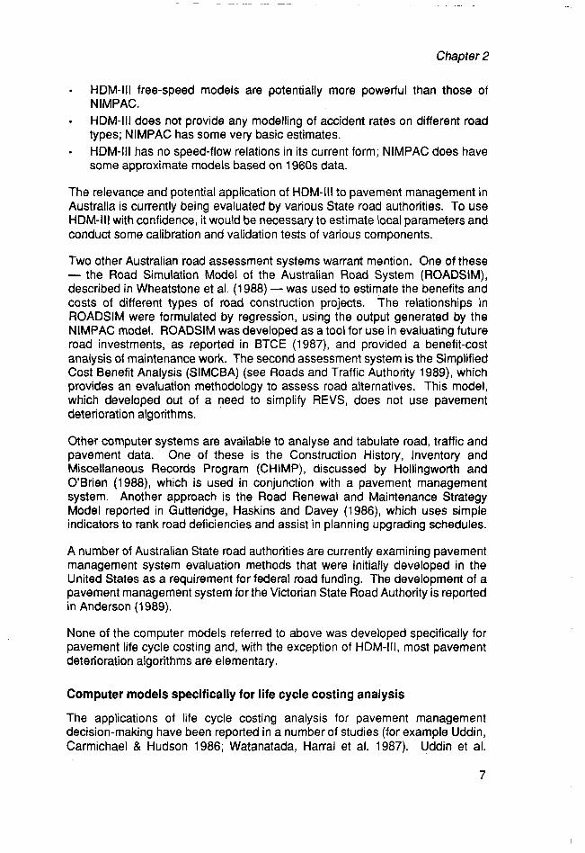
HDM-Ill free-speed models are potentially more powerful than those of NIMPAC. HDM-Ill does not provide any modelling of accident rates on different road types; NIMPAC has some very basic estimates. - HDM-Ill has no speed-flow relations in its current form; NIMPAC does have some approximate models based on 1960s data.
The relevance and potential application of HDM-Ill to pavement management in Australia is currently being evaluated by various State road authorities. To use HDM-Ill with confidence, it would be necessary to estimate local parameters and conduct some calibration and validation tests of various components.
Two other Australian road assessment systems warrant mention. One of these - the Road Simulation Model of the Australian Road System (ROADSIM), described in Wheatstone et al. (1 988) - was used to estimate the benefits and costs of different types of road construction projects. The relationships in ROADSIM were formulated by regression, using the output generated by the NIMPAC model. ROADSIM was developed as a tool for use in evaluating future road investments, as reported in BTCE (1987), and provided a benefit-cost analysis of maintenance work. The second assessment system is the Simplified Cost Benefit Analysis (SIMCBA) (see Roads and Traffic Authority 1989), which provides an evaluation methodology to assess road alternatives. This model, which developed out of a need to simplify REVS, does not use pavement deterioration algorithms.
Other computer systems are available to analyse and tabulate road, traffic and pavement data. One of these is the Construction History, Inventory and Miscellaneous Records Program (CHIMP), discussed by Hollingworth and OBrien (1988), which is used in conjunction with a pavement management system. Another approach is the Road Renewal and Maintenance Strategy Model reported in Gutteridge, Haskins and Davey (1986), which uses simple indicators to rank road deficiencies and assist in planning upgrading schedules.
A number of Australian State road authorities are currently examining pavement management system evaluation methods that were initially developed in the United States as a requirement for federal road funding. The development of a pavement management system for the Victorian State Road Authority is reported in Anderson (1 989).
None of the computer models referred to above was developed specifically for pavement life cycle costing and, with the exception of HDM-Ill, most pavement deterioration algorithms are elementary.
Computer models specifically for life cycle costing analysis
The applications of life cycle costing analysis for pavement management decision-making have been reported in a number of studies (for example Uddin, Carmichael & Hudson 1986; Watanatada, Harral et al. 1987). Uddin et al.
7
BTCE Occasional Paper 700
describe a life cycle costing program developed for the Pennsylvania Department of Transport. The program comprises both BASIC and FORTRAN components and provides for economic evaluation of a range of strategies for design and rehabilitation of road pavements. However, the pavement deterioration algorithm is somewhat simplistic. Further information on the use of life cycle costing techniques in the United States was collected by survey and reported in NCHRP (1985). Whilst 31 States confirmed that they use life cycle costing or similar techniques, most use basic pavement deterioration equations or performance curves. NCHRP (1 985,19) reported, ‘Most of these were developed for a given area or set of conditions and cannot be applied on any expanded basis. Further work is needed in this area’.
It was decided that it would be more effective to develop a pavement life cycle costing model incorporating the latest research on pavement deterioration, rather than to attempt to modify existing approaches.
DEVELOPMENT OF A LIFE CYCLE COSTING TECHNIQUE
Life cycle costing and pavement deterioration
Life cycle costing analysis is a valuable technique for making economic evaluations of competing funding strategies for road pavement design and maintenance. Each strategy should involve consideration of costs for initial construction, routine maintenance and rehabilitation, as well as of other items such as user benefits and vehicle operating costs.
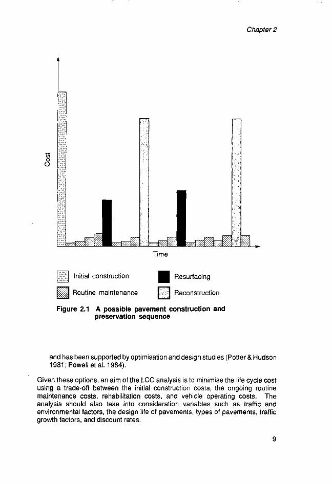
LCC analysis is not intended to generate new pavement designs. Design strategies can, however, be an important element of economic evaluation because they affect the initial construction costs, maintenance costs, vehicle operating costs and other user benefits. Figure 2.1 illustrates one possible pavement design and preservation strategy involving the scheduling of activities during the life of a pavement.
As reported in Lay (1986), to achieve a balanced strategy, the road pavement designer could be faced with a range of options, among them the following:
the construction of a pavement with a low initial cost, followed by frequent low cost strengthening by overlays - this option could be used when initial capital is limited but a steady flow of maintenance funds is available, and it could be considered as a staged-construction approach; the construction of a high quality pavement that reduces future maintenance costs and extends the time between major pavement rehabilitation operations -when funds are available, it may be appropriate to increase pavement life by increasing the pavement thickness and improving the quality of the initial construction; and the construction of a higher strength initial pavement, followed by frequent thin overlays-this approach will extend the time before major rehabilitation,
8
Chapter 2
...... 0 ..... . . . . Initial construction .... . . .
Time
Resurfacing ..... ..... ..... ..... Routine maintenance Reconstruction .....
Figure 2.1 A possible pavement construction and preservation sequence
and has been supported by optimisation and design studies (Potter & Hudson 1981 ; Powell et al. 1984).
Given these options, an aim of the LCC analysis is to minimise the life cycle cost using a trade-off between the initial construction costs, the ongoing routine maintenance costs, rehabilitation costs, and vehicle operating costs. The analysis should also take into consideration variables such as traffic and environmental factors, the design life of pavements, types of pavements, traffic growth factors, and discount rates.
9

CHAPTER 3 PAVEMENT DETERIORATION RELATIONSHIPS
The most important technical aspect of the development of a road pavement life cycle costing technique is the selection of a pavement deterioration algorithm - that is, a mathematical formula used to predict the deterioration of a pavement under typical Australian operating and environmental conditions.
In considering the life cycle of a road pavement, deterioration could be monitored using one or more of the following performance measures:
structural capacity; roughness; safety; riding comfort.
Pavement roughness
For the purpose of this study, roughness was adopted as the single most appropriate criterion for measuring road deterioration since this approach is recognised by both road users and State road authorities throughout Australia. It is also the approach adopted by overseas road authorities using pavement management systems. The importance of roughness as a primary measure of road condition is discussed in detail by Paterson (1 987, 15), who states:
Road roughness therefore emerges as a key property of road condition to be considered in any economic evaluation of design and maintenance standards for pavements, and also in any functional evaluation of the standards desired by road users.
There is a correlation between pavement roughness and riding comfort for users; in the future, riding comfort will be assessed by Australian road user panels as a measure of user satisfaction with the road pavement.
Pavement deterioration algorithms
In choosing roughness as the basis of adeterioration relationship for pavements, it was necessary to select an algorithm that reflected the increase in roughness over time and was consistent with practical Australian experience. The Bureau tested an initial selection of seven existing algorithms:
11

BTCE Occasional Paper 700
case 7 - a basic deterioration algorithm relating roughness to axle loadings and based on a concept discussed by Calvert (1 986); case 2- a simple algorithm relating future roughness to current roughness and based on an initial BTCE concept; case 3- an algorithm to extrapolate roughness over time using an existing roughness measure; - case 4 - an algorithm that was presented at the 1986 Australian Road Research Board conference (Paterson 1986), and which was subsequently developed and assessed as cases 5 and 7; case 5- the algorithm used in HDM-Ill (discussed in World Bank 1986); case 6- an algorithm specified by Parsley and Robinson (1 982); case 7- a later version of the Paterson (1986) algorithm, more adequately covering cracking and environmental deterioration (see Paterson 1987 for details).
Significant variables
When assessing a suitable deterioration algorithm for this study it was important to consider how the algorithm incorporated the major variables. For instance, Cox and Rolt (1986) note that pavement deterioration algorithms should desirably include terms relating to the following:
a change in traffic levels; the strength of the pavement; - an allowance for poor material quality;
. an allowance for the effect of the environment; rut occurrence and progression; crack occurrence and progression; and - pothole Occurrence and progression.
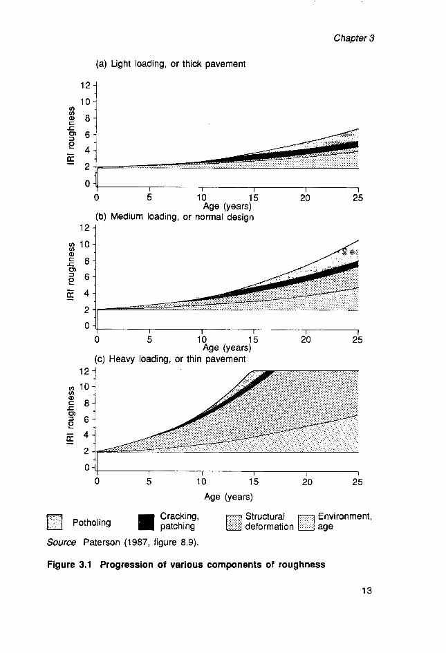
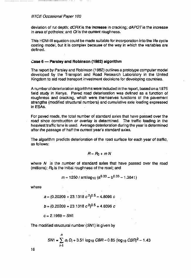
Figure 3.1 shows the impact of the various components of deterioration for pavements of differing strengths and traffic loadings. It shows the relative balance between environmental deterioration and deformation or structural or traffic deterioration for various pavement strengths. It also shows that patching and pothole components do not cause an increase in roughness until later years. The figure has been taken from Paterson (1 987) and is derived from the algorithm described as case 7.
ASSESSING THE ALGORITHMS
Each of the seven algorithms was assessed against: - the Cox and Rolt (1986) criteria listed in the preceding section; and
the guidelines outlined by NAASRA (1987b), which were used as a base to measure the adequacy of the algorithms in reflecting Australian road pavement, traffic and environmental conditions.
12
Chapter 3
(a) Light loading, or thick pavement
0 5 10 15 20 25 Age (years)
(b) Medium loading, or normal design
0 I
0 5 10 15 20 25
(c) Heavy loading, or thin pavement
I I I 1
Age (years)
0 0 5 10 15 20 25
l I I I l
Age (years)
Source Paterson (1987, figure 8.9).
Figure 3.1 Progression of various components of roughness
13
BTCE Occasional Paper 100
Case 1 - Calvert (1986) algorlthm
Calvert (1 986) presented a simple pavement deterioration algorithm:
R,,- R o + A n + B € S A C
where Rnis NAASRA roughness meter (NRM) counts per kilometre at yearn; R0 is initial NRM roughness (in counts per kilometre); n is time (in years) since construction; €SA is total equivalent standard axles after construction year n; and A, B and C are Coefficients.
This relationship was presented as a concept and the algorithm does not cover the major elements discussed by Cox and Rolt (1986). The regression coefficients proposed were unspecified, so further work would be required to calibrate them. This algorithm was explored by Loong and Miller (1989) but was not considered further in this work, because of the lack of a pavement strength parameter.
Case 2 - initial BTCE algorithm
The Bureau proposed a simple algorithm to undertake preliminary life cycle costing development. The algorithm is defined thus:
R"+, = A + B R , , ~
where Rn+l is roughness at year n + 1 ; A is annual roughness due to ageing; Rn is roughness at year n; and B and C are coefficients.
Coefficientsfor this algorithm were determined using the ratio of initial roughness to terminal roughness, selected as indicated by NAASRA (1987b, 49). As with case 1, the values of coefficients B and C were not specified, but they would probably be related to pavement strength or thickness.
Case 3 - roughness extrapolation algorithm
Case 3 provides an algorithm similar to that of case 2; it is used to extrapolate roughness change to a future date and is described by the Department of Transport and Works, Northern Territory (1989). The equation has the following form:
where Rn is roughness at year n; RC is current roughness; Rch is roughness change over a time period; tch is time period of roughness change Rch; tn is time to year n; and C is a coefficient, given as 1 . l 8 to approximate accelerating deterioration.
The first three algorithms (cases 1 ,2 and 3), which extrapoiate future roughness using existing roughness, may be satisfactory after calibration for specific road or traffic situations, but once calibrated for one road pavement they would not
14
Chapter 3
necessarily be applicable to other pavements. These three algorithms do not contain mathematical relationships for the pavement criteria specified by Cox and Rolt (1 986), so the Bureau rejected them.
Case 4 - Paterson (1986) algorithm
The equation described by Paterson (1986) provides an example of a long term roughness projection for pavements under good maintenance:
dRt = 648 (SNC + 1 )”.62 dNf4 + 0.1 20 dRDS + 0.0061 dCRX + 0.01 12 d f A T + 0.1 54 dVPOT + 0.0248 Rf t
where dRtis the increase in roughness over period t; Rt is the roughness at time t, in international roughness index (RI) units; dRDS is the increase in rut depth standard deviation of both wheelpaths; dCRXis the increase in indexed area of cracking; dPATis the increase in areaof surface patching; dVPOTis the increase in volume of open potholes per kilometre; t is the incremental time period of analysis (years); dNf4 is the incremental number of equivalent standard axles (ESA) in period t (million ESAs per lane); and SNC is the corrected structural number for pavement strength.
In this algorithm the measure of roughness used is the international roughness index ( M ) . The correlation between the NAASRA roughness meter (NRM) and IRI roughness measures is discussed in chapter 4.
The case 4 algorithm satisfies the Cox and Rolt (1986) criteria, including the structural, environmental and surface condition terms.
Case 5 -The HDM-Ill algorithm
The relationship used in HDM-Ill provides another algorithm for determining the change in roughness. The algorithm allows for the prediction of cracking, which influences deterioration in later years. Again, the equation uses structural, environmental and deterioration terms, and the similarity with other World Bank algorithms can be observed.
dQid =13Kgp[134fMT(SNCK+1)”~0YE4+0.114dRDS + 0.0066 dCRX + 0.42 &POT] + Kge 0.023 QI
where dQid is the predicted change in road roughness during the analysis year due to road deterioration; Kgp is the user-specified deterioration factor for roughness progression (default value is 1); EMT is 2.71 8°.023 Kge AGB; Kge is the user-specified deterioration factor for the environment-related annual fractional increase in roughness (default value is 1); AGE3 is pavement age; SNCKis the modified structural number adjusted for the effect of cracking, based on SNK (SNK is the predicted reduction in the structural number due to cracking since the last pavement reseal, overlay or reconstruction based on the predicted excess cracking beyond the amount that existed in the old surfacing layers); YE4 is the annual number of equivalent axle loads; dRDS is the increase in standard
15
BTCE Occasional Paper 700
deviation of rut depth; dCRXis the increase in cracking; dAPQTis the increase in area of potholes; and Q/ is the current roughness.
This HDM-Ill equation could be made suitable for incorporation into the life cycle costing model, but it is complex because of the way in which the variables are defined.
Case 6 - Parsley and Robinson (1982) algorithm
The report by Parsley and Robinson (1982) outlines a prototype computer model developed by the Transport and Road Research Laboratory in the United Kingdom to aid road transport investment decisions for developing countries.
A number of deterioration algorithms were included in the report, based on a 1975 field study in Kenya. Paved road deterioration was defined as a function of roughness and cracking, which were themselves functions of the pavement strengths (modified structural numbers) and cumulative axle loading expressed in ESAs.
For paved roads, the total number of standard axles that have passed over the road since construction or overlay is determined. The traffic loading in the heaviest traffic lane is used. Average deterioration during the year is determined after the passage of half the current year's standard axles.
The algorithm predicts deterioration of the road surface for each year of traffic, as follows:
R = R o + m N
where N is the number of standard axles that have passed over the road (millions); R0 is the initial roughness of the road; and
m = 1250 / antiloglo (ao.as - - 1.3841)
where
a = (0.20209 + 23.1 31 8 G ~ ) ~ . ~ - 4.8096 C
b = (0.20209 + 23.131 8 c ~ ) ~ . ~ + 4.8096 C
C = 2.1 989 - SN1
The modified structural number (SNl) is given by
Chapter 3
where ajis the strength coefficient of layer i; Djis the thickness of layer i(inches); CBR is the California bearing ratio of the subgrade; and where, for bituminous surfacings, aiis the AASHO strength coefficient - for road bases
ai= (29.14 CBRi - 0.1 977 CBRi2 + 0.00045 CBRj3) lo4 and for sub-bases
ai= 0.01 + 0.065 log10 (CBRj)
where CBRiis the California bearing ratio of the layer i.
In this algorithm the input data could not be directly related to the requirements of the NAASRA pavement design manual. There was also uncertainty about the relationship between the California bearing ratio and pavement stiffness for Australian conditions.
As with the HDM-Ill equation (case 5), this algorithm lacked some 'user friendliness' owing to the way in which variables were specified. Other algorithms require less data and were more appropriate.
Case 7 - Paterson (1 987) Algorithm
Following the most recent Paterson algorithm (Paterson 1987, equation 8.13), which is described as a component algorithm:
dRt = 134 e"' SNCK5.0 dNf4 + 0.1 14 dRDS + 0.0066 dCRX + 0.003 Hp dPAT + 0.16 dVPOT+ m Rt dt
where dRtis the increase in IRI roughness over time period t; Rtis the roughness at time t(metres per kilometre IRI); t is the age of pavement or overlay (years); m is the environmental coefficient; dNf4 is the incremental number of equivalent standard axles in period cff (million ESAs per lane); dRDS is the increase in rut depth standard deviation of both wheelpaths (millimetres); dCRXis the increase in area of cracking (per cent); Hp is the patch protrusion (millimetres); dPATis the increase in area of surface patching (per cent); dVPOT is the increase in volume of open potholes (millimetres per lane-kilometre); dt is the incremental time period of analysis (years); and
SNCK= 1 + SNC- 0.0000758 H CRX
where SNC is the modified structural number of pavement strength; H is the thickness of cracked layer (millimetres); and CRX is the area of cracking (per cent).
This algorithm seemed the most satisfactory for use in Australia for several reasons:
the way in which it satisfies the Cox and Rolt (1 986) criteria for traffic, pavement strength, environment, rutting and cracking;
17
BTCE Occasional Paper 7 00
its relative simplicity; and . it represents the compilation of the results of extensive World Bank work.
The algorithm was superior to the other six algorithms. It is also in a form suitable for incorporation in a computer spreadsheet model designed to increment roughness year by year.
?ne Paterson aggregate algorithm
It is important to note that Paterson specified an aggregate roughness trend algorithm that is described as a suitable alternative to the case 7 component algorithm for general pavement life estimates. The aggregate model (equation 8.20 in Paterson 1987), has the following form:
Rlt = [ RIO + 725 (SNC + 1 )4.99 NE+ ] eo.01 53
where R/t is the roughness at time t (metres per kilometre IRI); RIO is the roughness at time 0 (metres per kilometre IRI); NE4tis the cumulative equivalent standard axles until time t (million ESAs per lane); t is the age of the pavement since overlay or construction; and SNC is the modified structural number.
Paterson advises that this equation should be used only for flexible pavements without extensive cracking, and that empirical evidence suggests that an indicator of surface distress could be incorporated to enhance the predictive accuracy of this simplified algorithm. The structure of the algorithm can provide guidance on the emphasis for subsequent refinement.
THE ALGORITHM AND AUSTRALIAN CONDITIONS
The Bureau subsequently undertook work to ensure that the case 7 algorithm matched Australian conditions and road pavement data-collection arrangements.
Australian pavement data collection
As a component of their pavement management systems, Australian State road authorities are expected to collect data on roughness, rutting, cracking and surface texture. Surface texture changes are not considered as a predictor variable for pavement deterioration. The following measures are expected to be used: . rutting - ruts greater than 20 millimetres deep; and
cracking - cracks of any type more than 2 millimetres wide.
The measure of severity is expected to be defined thus: class 0- occasional, isolated or not present; class 7 - intermittent; and class 2- continuous, widespread.
Many local government authorities are also starting to collect pavement data.
18
Chapter 3
Rutting In Australia rutting is generally defined in terms of the proportion of pavement length with ruts greater than a specified depth. It has been assumed that any increase in rutting length is likely to be related to any increase in the case 7 rut depth, and for this reason the term dRDS has been replaced with dRDL as a measure of rutting length. The rutting coefficient was reduced to match the proportion of rutting length rather than the standard deviation of rut depth. Understanding of the contribution of this factor to pavement deterioration is expected to improve with further research.
Pavement strength Pavement strength, which is directly related to a Benkelman beam (or similar) deflection measure, is the most difficult measure to obtain, particularly for the investigation of road systems. Methods to provide approximate strength measures are discussed in chapter 4.
Patching and potholes The patching and pothole terms in the case 7 algorithm require further consideration because the area patched is more a measure of work undertaken than of pavement deficiency. In any case, Paterson (1 987) notes that potholing tends to cause only a small contribution to pavement deterioration, with the effect not being realised until later years as shown in figure 3.1. This variable is expected to have even less impact in Australia, where road standards are high is comparison with the developing countries in which the research was undertaken. The case 7 algorithm was assessed to ensure that it predicted the pavement design expected by NAASRA (1 987b).
Cracking It is assumed that under Australian conditions cracks wider than 2 millimetres would be the most appropriate cracking measure. These generally correspond to the class 1 and 2 cracks noted in Paterson’s equation 5.3 ( 1 987). The rate of progression of cracking specified by Paterson’s figure 5.1 (c) is considered appropriate for Australian conditions.
For the time until the first crack, Paterson’s equation 5.28(a) is considered appropriate and has been used in this work:
Time until first crack = 13.2 e(-20.7 dNE4’sNc2)
using the variables as previously defined.
Australian algorithm
The roughness algorithm, based on Paterson’s ( 1 987) equation 8.1 3 modified to suit Australian conditions, is as follows:
dRt = 134 P‘ SNCK5.’ dNE4 + 0.01 2 dRDL + 0.0066 dCRX + m Rtdf + (0.003 Hp dPAT+ 0.16 dVPOT)
19

BTCE Occasional Paper 100
where dRDL is the increase in occurrence of 20 millimetre rutting, expressed as a percentage of the total wheel path length; and dCRX is the increase in percentage of pavement area of the occurrence of intermittent cracks wider than 2 millimetres.
The Paterson patching and pothole variables are optional since the accuracy of the result is influenced little by their omission. The coefficients for the Australian parameters dRDL and dCRX are expected to be refined further as more information becomes available. The equation in this form should provide a higher level of accuracy than the Paterson aggregate algorithm because it incorporates rutting, cracking and environmental terms.
The Bureau has incorporated the foregoing algorithm into a computer-based spreadsheet model capable of analysing the deterioration of flexible road pavements. It is anticipated that this equation will be developed further and calibrated as pavement management systems become more widely used and as Australian pavement deterioration is further researched. The algorithm is proposed as a base; it is expected to be continuously improved as data become available.
20
CHAPTER 4 DESCRIPTION OF THE LIFE CYCLE COSTING COMPUTER MODEL
This chapter discusses the development of the BTCE life cycle costing computer model, which provides the means of utilising the Australian pavement deterioration algorithm developed in chapter 3.
As noted in chapter 2, the Bureau developed a new computer program rather than modifying an existing model such as NIMPAC or HDM-Ill. It did this for a number of reasons:
The approach had to reflect the pavement and traffic interaction, rather than addressing the wider road location, alignment and capacity issues.
- The approach had to reflect the impact of the environment on the deterioration of road pavements, which can be a deciding factor for pavement life, particularly under low traffic conditions. The computer model was required to incorporate an Australian algorithm and conditions. Flexible computer spreadsheets with the potential for easy modification and integration with pavement management systems were available.
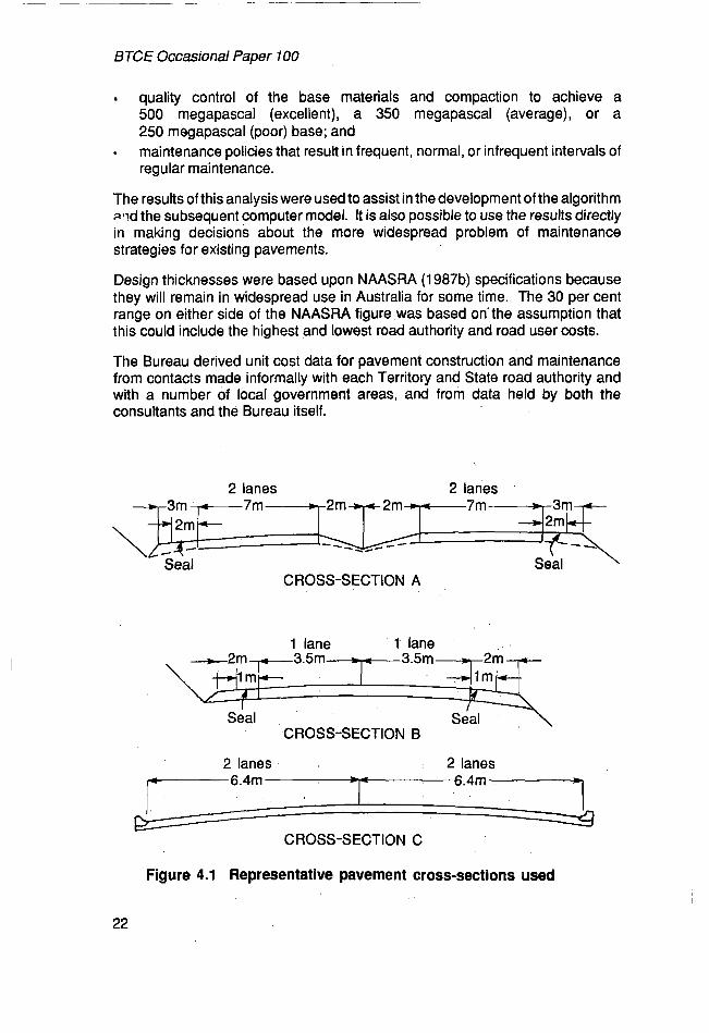
As part of the initial testing of the approach, the Bureau checked annual pavement construction, maintenance and rehabilitation costs over a forty-year period for a range of traffic, environmental and maintenance strategy conditions. Rather than attempting to tabulate every combination of flexible pavement width, the Bureau chose three road cross-sections, representing more than 90 per cent of Australian roads and providing for shoulder as well as travelled pavement influences. Figure 4.1 shows the three representative cross-sections used.
The computer model can be used in deciding pavement construction and maintenance strategies for new and existing roads. I t can be used to assess a wide variety of options; the tabulations and appendices in this report provide examples of some of the possibilities for decision-making, using the life cycle costing approach, for:
pavement of NAASRA design thickness (as per NAASRA 1987b) and
flush bituminous seal surfacing or asphalt concrete surfacing; pavements that are up to 30 per cent thicker or thinner than that thickness;
21
BTCE Occasional Paper 100
quality control of the base materials and compaction to achieve a 500 megapascal (excellent), a 350 megapascal (average), or a 250 megapascal (poor) base; and maintenance policies that result in frequent, normal, or infrequent intervals of regular maintenance.
The results of this analysis were used to assist in the development of the algorithm sild the subsequent computer model. It is also possible to use the results directly in making decisions about the more widespread problem of maintenance strategies for existing pavements.
Design thicknesses were based upon NAASRA (1 987b) specifications because they will remain in widespread use in Australia for some time. The 30 per cent range on either side of the NAASRA figure was based onsthe assumption that this could include the highest and lowest road authority and road user costs.
The Bureau derived unit cost data for pavement construction and maintenance from contacts made informally with each Territory and State road authority and with a number of local government areas, and from data held by both the consultants and the Bureau itself.
2 lanes 2 lanes -3m = 7m
Seal CROSS-SECTION A
1 lane 1 lane
Seal CROSS-SECTION B
2 lanes 2 lanes
CROSS-SECTION C
Figure 4.1 Representative pavement cross-sections used
22
Chapter 4
Construction cost data were more abundant and reliable than maintenance cost data. Nevertheless, the data sets represent a reasonable ‘average’ cost. Users of a computer-based life cycle costing model can supply actual cost and other parameters fitting their particular conditions.
Research undertaken during this phase of the study revealed that no single algorithm accounted accurately for all pavement serviceability parameters and that it may be many years before any greatly improved algorithms are developed and tested.
The computer deterioration model
In order to use the Australian road deterioration algorithm described in chapter 3, the Bureau developed a computer spreadsheet model incorporating the following features:
a method of specifying the contribution each variable makes towards the pavement roughness; an environmental factorthat can be set to accommodate arid, normal or humid conditions; a series of local calibration factors to enable the model to be tuned to meet specific local conditions and to improve its sensitivity; and
- a graphic output to permit an examination of the results.
Initial assumptions were made in the spreadsheet model as to the improvement in pavement roughness and strength due to various maintenance options. These preliminary estimates have been based on NAASRA (1 987b). Users of the LCC model can easily change these parameters if necessary. The Bureau designed the model for use with commercially available computer spreadsheet comprising the following ten modules:
module 7 - road length; module 2 - traffic; module 3- existing pavement condition;
- module 4- proposed pavement condition; module 5- intervention points; module 6- impact of intervention; module 7- local calibration factors; module 8- construction and maintenance costs; - module 9- vehicle operating cost;
. module 70- net present value.
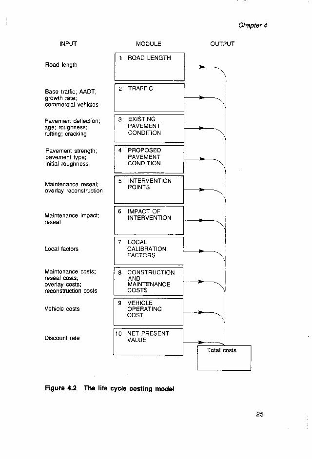
Figure 4.2 shows a schematic layout of the model and the relationship of the modules. The spreadsheet model has a number of features:
9 It can examine existing roads and assist in assessing future maintenance and It assesses unit road sections sequentially.
reconstruction options, as well as investigating proposed roads.
23
BTCE Occasional Paper 100
. It can easily be rearranged to operate using database information and to analyse road systems made up of multiple sections.
. It is based on the assumption that the section of road being examined has uniform properties. If the section under consideration is not homogeneous, the model can be reconfigured or shorter sections created.
The algorithm and the model are applicable to flexible bituminous pavements. The model can provide a base for the necessary research for Australian concrete and unsealed pavements.
The remainder of this chapter follows the logic of the computer spreadsheet model and describe the model’s ten components.
ROAD LENGTH AND TRAFFIC MODULES
Modules 1 and 2 provide a profile of traffic over a forty-year period for a number of vehicle types. Data required include the estimated annual average daily traffic, the number of traffic lanes, traffic composition and the traffic growth rate for each vehicle type. From this profile, the equivalent standard axles of the traffic can be calculated. The equivalent standard axle (ESA) rating for a vehicle is a measure of the relative effect of any load and axle configuration on a road pavement in terms of the number of passes of a standard reference axle. The number of ESAs is calculated using the relationships provided by NAASRA (1 987b, ch. 7).
EXISTING AND PROPOSED PAVEMENT CONDITION MODULES
The spreadsheet model can be used to analyse the following: . existing pavements, where information on the existing pavement will be
required as input to the model; existing pavements that are expected to be replaced by new pavements after a period of time has elapsed, where both the existing and the proposed pavement details will be required; and
- completely new pavements, where only new pavement information will be required as input to the model.
For existing pavements, parameters such as the current pavement strength must be measured. For proposed pavements, pavement strength will need to be calculated.
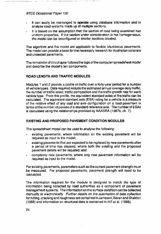
The information required for the module is designed to match the type of information being collected by road authorities as a component of pavement management systems. The information on the surface condition can be collected manually or electronically. Further details on the automation of data collection for rutting, cracking and roughness arecontained in Jameson, Baran and Sheldon (1988) and information on structural data is contained in Hill et al. (1988).
24
INPUT MODULE
Chapter 4
OUTPUT
Road length 1 ROAD LENGTH l-
Base traffic; AADT; growth rate; commercial vehicles
2 TRAFFIC t” Pavement deflection; age; roughness; rutting; cracking
3 EXISTING PAVEMENT CONDITION t”
Pavement strength; pavement type; initial roughness
4 PROPOSED PAVEMENT CONDITION
Maintenance reseal; overlay reconstruction
Maintenance impact; reseal
Local factors
Maintenance costs; reseal costs; overlay costs; reconstruction costs
Vehicle costs
Discount rate
I 5 INTERVENTION I
I PolNTS t“ 6 IMPACT OF
INTERVENTION
7 LOCAL ’i I
CALIBRATION FACTORS
l 1 ! 8 CONSTRUCTION
AND MAINTENANCE COSTS
I l
I 9 VEHICLE 1 i OPERATING 1 COST
1 I
VALUE
Figure 4.2 The life cycle costing model
25
BTCE Occasional Paper 100
Roughness
For existing pavements, roughness is measured; for proposed pavements the initial roughness is estimated. The model will calculate the subsequent roughness deterioration.
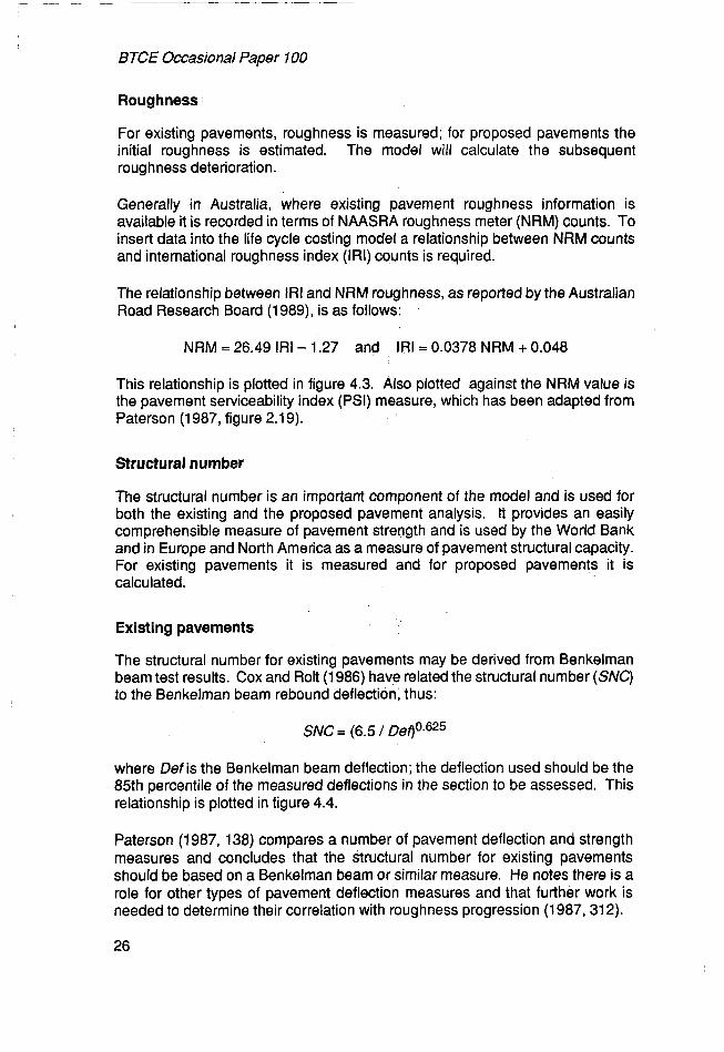
Generally in Australia, where existing pavement roughness information is available it is recorded in terms of NAASRA roughness meter (NRM) counts. To insert data into the life cycle costing model a relationship between NRM counts and international roughness index (IRI) counts is required.
The relationship between IRI and NRM roughness, as reported by the Australian Road Research Board (1 989), is as follows:
NRM = 26.49 IRI - 1.27 and IRI = 0.0378 NRM + 0.048
This relationship is plotted in figure 4.3. Also plotted against the NRM value is the pavement serviceability index (PSI) measure, which has been adapted from Paterson (1 987, figure 2.1 9).
Structural number
The structural number is an important component of the model and is used for both the existing and the proposed pavement analysis. It provides an easily comprehensible measure of pavement strength and is used by the World Bank and in Europe and North America as a measure of pavement structural capacity. For existing pavements it is measured and for proposed pavements it is calculated.
Existing pavements
The structural number for existing pavements may be derived from Benkelman beam test results. Cox and Rolt (1986) have related the structural number (SNC) to the Benkelman beam rebound deflection, thus:
SNC = (6.5 f Det)Q.625
where Defis the Benkelman beam deflection; the deflection used should be the 85th percentile of the measured deflections in the section to be assessed. This relationship is plotted in figure 4.4.
Paterson (1987, 138) compares a number of pavement deflection and strength measures and concludes that the structural number for existing pavements should be based on a Benkelman beam or similar measure. He notes there is a role for other types of pavement deflection measures and that further work is needed to determine their correlation with roughness progression (1987, 312).
26

8 -
7-
- 6 - v> a
- 1 , / PS I
I / - \
0 30 60 90 1 2 0 150 160 2 io 240 NRM
Figure 4.3 IRI, NRM and PSI roughness comparison
71
I I I I I 1 I I I l
1 1.5 2 2.5 3 3.5 4 4.5 5 5.5 6 Structural number
Figure 4.4 Relationship of structural number to deflection
27

BTCE Occasional Paper 100
Proposed pavements
The module for proposed pavements contains the details of the pavement proposal. As with the existing pavement, certain parameters are required. Again, the structural number is needed; it may be calculated by either mechanistic analysis or empirical analysis.
For the mechanistic analysis, computer programs such as CIRCLY or ELSYM5 would be used to determine the surface deflection. This analysis requires the input of the modulus of the expected pavement materials and layer thicknesses. This approach is described further by NAASRA (1987b). Appendix I presents results of such analyses for a number of traffic and pavement options.
In the case of empirical analysis, the method assumes that a pavement was designed as outlined by NAASRA (1987b) and uses figure 10.3, 'Design deflection against design traffic', of that document. The approximate structural numbercan be calculated from the design surface deflection for the design traffic. Figure 4.5 of this paper plots the relationship. Regression analysis of the relationship provides the following equation:
SNC = 0.40 log DT+ 3.00
where SNC is the structural number and DTis the design traffic for 20 years (million ESAs). This empirical analysis is not as accurate as the mechanistic analysis.
1.8 ! I I 1 I I
1 000 10 000 100 000 1 000 000 10 000 000 100 000 000 Traffic for 20 years (ESAs)
Figure 4.5 Structural number versus design traffic
28
Chapter 4
Change in pavement strength over time
For either an existing or a proposed pavement, the LCC spreadsheet model will calculate any deterioration in pavement strength using the relationship defined by Paterson (1987, equation 8.11), where pavement strength (SNC) is progressively reduced (to become SNCK) after the onset of cracking. The time expected until the first crack is discussed in chapter 3.
Pavement rutting and cracking
It is necessary to provide information about the rutting and cracking of an existing pavement. The measure for the extent of rutting is as follows:
increase in occurrence of rutting greater than 20 millimetres deep, expressed as a percentage of the total wheel path length.
For cracking, the measure is as follows: increase in percentage of pavement area where intermittent cracks greater than 2 millimetres wide occur.
Both these measures will coincide with the AUSTROADS (1989) proposals for the surface condition and pavement condition indices used as components of the State road authorities pavement management systems.
Change in rutting and cracking over time
The model will calculate changes in rutting and cracking for either existing or proposed pavements, in increments of one year. For proposed pavements, it is expected that the rutting will follow the deterioration patterns specified by Paterson (1987) in equation 7.1 1 and that the cracking will follow his specifications in equation 5.28 and figure 5.1 (c). For existing pavements the current rutting and cracking (if any) is specified as an input, with future rutting and cracking determined within the model, following the patterns already noted.
INTERVENTION POINTS MODULE
Maintenance triggers
The intervention points module of the spreadsheet model allows the testing of the effectiveness of various activities such as maintenance, resealing, and resheeting or overlay. The trigger for the commencement of these works could be time-based or roughness-based.
When developing this work, after a relationship for pavement deterioration had been determined it was necessary for the Bureau to define the level of deterioration at which a maintenance activity should be initiated. In the case of simple reseals, which have little impact upon roughness, a purely time-based maintenance trigger would be the most realistic and suitable.
29
BTCE Occasional Paper 700
TABLE 4.1 POSSIBLE INTERVENTION BASED ON IRI ROUGHNESS CRITERIA
/R/ Roughness prior W k m ) Acfion fo intervention
0-2 DO nothing Very satisfactory
2-3 Preventative maintenance Satisfactory (rejuvenation, reseal)
3-4 Corrective maintenance Poor (shape correction)
4-6 Rehabilitation Barely tolerable
6+ Reconstruction Unsatisfactory
TABLE 4.2 POSSIBLE INTERVENTION BASED ON NAASRA ROUGHNESS CRITERIA
Roughness (NRM counts/km)
Cross-section A Cross-section B Cross-section C Action
<50 458 <68 Do nothing
50-69 60-79 65-84 Preventive maintenance (rejuvenation, reseal)
90-1 19 100-119 ,l 05-1 24 Corrective maintenance (shape correction)
11 0-149 150-1 69 170-189 ' Rehabilitation (structural)
150+ 170+ 190+ Reconstruction
Cross-sections A, B, C: see figure 4.1
TABLE 4.3 POSSIBLE TIME-BASED MAINTENANCE TRIGGERS
Trigger pattern (years)
Maintenance lnfrequent Normal Frequent
Routine Rejuvenation or enrichment Reseal or thin overlay
5 3
7 5
15 10
30
Chapter 4
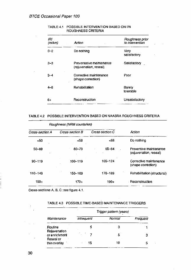
The flexibility of the LCC model allows differing maintenance strategies to be tested. The designer can try various options, some of which are shown in tables 4.1 and 4.2.
The roughness-based criteria can be described in the model input data in terms of IRI or NRM counts.
Time-based maintenance triggers used in the model could apply to routine maintenance, rejuvenation or enrichment, and reseal or thin overlay. Routine maintenance includes pothole and edge patching. Rejuvenation or enrichment could include a light bitumen emulsion spray or equivalent, and reseal or thin overlay could include a hot bitumen seal or a thin asphalt concrete overlay. Table 4.3 shows three time-based patterns that could be built into the model. The LCC model provides an opportunity for assessing the interaction and implications of various time-based and condition-based strategies.
The figures in table 4.3 are provided as a guide; the model can easily be set up to accommodate particular conditions. Use of the LCC model is expected to improve understanding of the optimum time to commence maintenance intervention activities.
IMPACT OF INTERVENTION MODULE
For module 6 the details of the expected improvements in the pavement condition following maintenance works are entered. For example, a reseal would be expected to have an impact on cracking, to have a minimal impact on the immediate pavement roughness and strength, but to have an impact on pavement life. Agranularorasphalt overlay, on the other hand, would have a positive impact on pavement strength, roughness and pavement life.
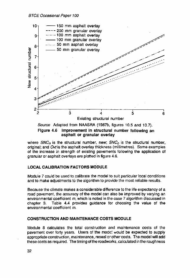
Granular overlays and structural numbers
The improvement in the structural number of an existing pavement after a granular overlay treatment, can be assessed using figure 10.5 of NAASRA (1987b) and figure 4.4 .of this paper. The improvement in strength can be calculated from the following equation:
where SNCn is the structural number, new; SNC, is the structural number, original; and Ovtk the granular overlay thickness (millimetres).
SNCn = SNCO [l /(l - 0.0024 Ovt)]0,625
Asphalt overlays and structural numbers
The improvement in the structural number of an existing pavement after an asphalt overlay treatment can be assessed using figure 10.7 of NAASRA (1 987b) and figure 4.4 of this paper. The improvement in strength can be calculated from the following equation:
SNCn = SNCo [l/(l - 0.00323 Ovt)]0.625
31
BTCE Occasional Paper 100
10- - 150 mm asphalt overlay "" 200 mm granular overlay
9- 100 mm asphalt overlay
& 50 mm granular overlay
z 7
- 100 mm granular overlay "'. '" ' 50 mm asphalt overlay 8-
E -
E 3 6-
a
- c 0 3 L
2 I 1 I 1
2 3 4 5 6 Existing structural number
Source Adapted from NAASRA (1987b, figures 10.5 and 10.7). Figure 4.6 Improvement in structural number following an
where SNC, is the structural number, new; SNC, is the structural number, original; and Ovt is the asphalt overlay thickness (millimetres). Some examples of the increase in strength of existing pavements following the application of granular or asphalt overlays are plotted in figure 4.6.
asphalt or granular overlay
LOCAL CALIBRATION FACTORS MODULE
Module 7 could be used to calibrate the model to suit particular local conditions and to make adjustments to the algorithm to provide the most reliable results.
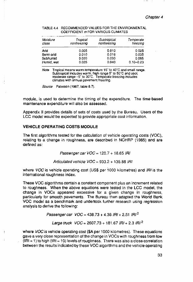
Because the climate makes a considerable difference to the life expectancy of a road pavement, the accuracy of the model can also be improved by varying an environmental coefficient m, which is noted in the case 7 algorithm discussed in chapter 3. Table 4.4 provides guidance for choosing the value of the environmental coefficient m.
CONSTRUCTION AND MAINTENANCE COSTS MODULE
Module 8 calculates the total construction and maintenance costs of the pavement over forty years. Users of the mode! would be expected to supply appropriate construction, maintenance, reseal or other costs. The model will add these costsas required. The timing of the roadworks, calculated in the roughness
32
Chapter 4
TABLE 4.4 RECOMMENDED VALUES FOR THE ENVIRONMENTAL COEFFICIENT m FOR VARIOUS CLIMATES
Moisture Tropical Subtropical Temperate class nonfreezing nonfreezing freezing
Arid 0.005 0.01 0 0.025 Semi-arid 0.01 0 0.01 6 0.035 Subhumid 0.020 0.030 0.065 Humid, wet 0.025 0.040 0.10-0.23
Note Tropical means warm temperature 15' to 40'C and small range. Subtropical includes warm, high range 5'to 50'C and cool, moderate range -5' to 30%. Temperate freezing includes climates with annual pavement freezing.
Source Paterson (1987, table 8.7).
module, is used to determine the timing of the expenditure. The time-based maintenance expenditure will also be assessed.
Appendix I I provides details of sets of costs used by the Bureau. Users of the LCC model would be expected to provide appropriate cost information.
VEHICLE OPERATING COSTS MODULE
The first algorithms tested for the calculation of vehicle operating costs (VOC), relating to a change in roughness, are described in NCHRP (1985) and are defined as:
Passenger c a r VOC = 120.7 + 18.65 1/31
Articulated vehicle VOC = 933.2 + 135.88 IRI
where VOC is vehicle operating cost (US$ per l000 kilometres) and /RI is the international roughness index.
These VOC algorithms contain a constant component plus an increment related to roughness. When the above equations were tested in the LCC model, the change in VOCs appeared excessive for a given change in roughness, particularly for smooth pavements. The Bureau then adapted the World Bank VOC model as a benchmark and undertook further research using regression analysis to derive the following:
Passenger car VOC = 438.73 + 4.38 IRI + 2.51 /RI2
Large truck VOC = 2607.73 + 181.67 IRI + 2.3 IRI
where VOC is vehicle operating cost ($A per 1000 kilometres). These equations gave a very close representation of the change in VOCs with roughness from low (IRI = 1) to high (IRI = 10) levels of roughness. There was also aclose correlation between the results indicated by these VOC algorithms and the vehicle operating
33
BTCE Occasional Paper 100
costs of Australian cars reported in NRMA (1 989). Regression analysis was also undertaken for other vehicle types. A simple VOC model described by Ullidtz (1 983) assisted in the calibration of the derived VOC algorithms.
Details of the work of the World Bank on this subject are contained in World Bank (1986, 1988). Further information on the use of vehicle operating costs as a component of road assessment systems is contained in Satish and Lingras (1 989).
The present VOC module does not include travel time costs for drivers, passengers or freight.
A more complex computer model would be required if issues such as congestion, accident and traffic delay costs due to roadworks were to be incorporated. Road realignments, urban areas, non-pavement expenditure and bridges would represent further levels of complexity. The sensitivity of vehicle operating costs to road roughness and vehicle speeds is an area where further research is warranted.
NET PRESENT VALUE MODULE
The model currently uses the net present value method (module 10) to calculate total road.authority costs and the total vehicle operating costs. These two major costs can be summed and it is expected that the minimisation of both road authority costs and vehicle operating costs will be an important application for the LCC model.
Maintenance benefit-cost ratio
The model also calculates a benefit-cost ratio using the reduction in the net present value of vehicle operating costs (base case less improved case) as the benefits, divided by the net present value reduction in the total authority costs. There are conceptual problems associated with determining a benefit-cost ratio for maintenance work: it is difficult to quantify the benefits of activities such as routine maintenance. Another problem is the determination of what is the base maintenance case against which to compare alternative strategies. In the LCC model the base case is calculated allowing for an increase in roughness up to the reconstruction trigger point (or the initial roughness level if that was greater) and calculating the vehicle operating costs up to, and then at, that level. The base case allows for routine maintenance only and does not include any resealing, resheeting or reconstruction. The routine maintenance level can also be increased at high roughness levels. Because of the flexibility of the LCC model, all assumptions can be quickly checked. Chapter 5 deals with the issue in greater detail.
34

CHAPTER 5 OUTPUTS AND APPLICATION OF THE LIFE CYCLE COSTING MODEL
The Bureau incorporated the work discussed in chapter 4 in a spreadsheet computer program so that its research will have a practical application. With the growth in personal computers, spreadsheets are now widely used; they are powerful tools, particularly for answering the ‘What if?’ questions. Use of a spreadsheet-based model eliminates many computer coding problems, and the software is documented. Because the model incorporates off-the-shelf cornputer software it can easily function as a framework that can be rearranged. Another virtue of the model is its simplicity.
USE OF THE MODEL FOR PAVEMENT LIFE ASSESSMENT
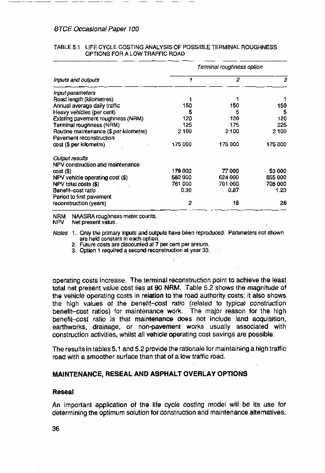
Table 5.1 illustrates the operation of the life cycle costing model. The options used are three typical road pavements, each 1 kilometre long. The LCC model is used to assess differing pavement construction and maintenance strategies. The first comparison for a typical low traffic volume road examines differing terminal roughness options.
As the terminal roughness increases - which will reduce the discounted construction and maintenance costs - the vehicle operating costs will increase. The terminal reconstruction point to achieve the least total net present value cost lies at 180 NRM.
Because there are benefits to be gained from reconstructing higher traffic roads at lower roughness levels, a set of curves could be produced to indicate optimum reconstruction points against various traffic levels.
The vehicle operating costs shown in table 5.1 increase by only 21 per cent over the roughness range shown because other factors contribute to the costs. Figure 5.1 provides a diagrammatic representation of the options shown in the table. The figure shows that roughness increases until the prescribed trigger point is reached, at which point the pavement is reconstructed.
Table 5.2 presents a similar case, a high traffic, divided road with a heavier pavement. As in table 5.1, as the terminal roughness increases - which will reduce the discounted construction and maintenance costs - the vehicle
35
BTCE Occasional Paper 7 00
TABLE 5.1 LIFE CYCLE COSTING ANALYSIS OF POSSIBLE TERMINAL ROUGHNESS OPTIONS FOR A LOW TRAFFIC ROAD
Terminal roughness option
Inputs and outputs l 2 3
Input parameters Road length (kilometres) 1 1 1 Annual average daily traffic 150 150 150 Heavy vehicles (per cent) 5 5 5 Existing pavement roughness (NRM) 120 120 120 Terminal roughness (NRM) 125 1 75 225 Routine maintenance ($ per kilometre) 2 100 2 100 2 100 Pavement reconstruction cost ($ per kilometre) 175 000 175 000 175 000
Output results NPV construction and maintenance
NPV vehicle operating cost ($) 582 000 624,000 655 000 NPV total costs ($) 761 000 701 000 708 000 Benefitast ratio 0.30 0.87 1.23 Period to first pavement reconstruction (years) 2 18 26
NRM NAASRA roughness meter counts. NPV Net present value.
Notes 1. Only the primary inputs and outputs have been reproduced. Parameters not shown
cost ($1 179 000 77 000 53 000
are held constant in each option. 2. Future costs are discounted at 7 per cent per annum. 3. Option 1 required a second reconstruction at year 33.
operating costs increase. The terminal reconstruction point to achieve the least total net present value cost lies at 90 NRM. Table 5.2 shows the magnitude of the vehicle operating costs in relation to the road authority costs; it also shows the high values of the benefit-cost ratio (related to typical construction benefit-cost ratios) for maintenance work. The major reason for the high benefit-cost ratio is that maintenance does not include land acquisition, earthworks, drainage, or non-pavement works usually associated with construction activities, whilst all vehicle operating cost savings are possible.
The results in tables 5.1 and 5.2 provide the rationale for maintaining a high traffic road with a smoother surface than that of a low traffic road.
MAINTENANCE, RESEAL AND ASPHALT OVERLAY OPTIONS
Reseal
An important application of the life cycle costing model will be its use for determining the optimum solution for construction and maintenance alternatives.
36
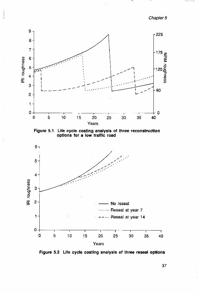
Chapter 5
3
2
0 ' L O 0 5 10 15 20 25 30 3 5 4 0
Years
Figure 5.1 Life cycle costing analysis of three reconstruction options for a low traffic road
- No reseal . . . . . . . Reseal at year 7
"" Reseal at year 14
I I I I I I I I
0 5 10 15 20 25 30 35 40
Years
Figure 5.2 Life cycle costing analysis of three reseal optlons
37

BTCE Occasional Paper 7 00
TABLE 5.2 LIFE CYCLE COSTING ANALYSIS OF POSSIBLE TERMINAL ROUGHNESS OPTIONS FOR A HIGH TRAFFIC DIVIDED ROAD
Terminal roughness option
Inputs and outputs l 2 3
Input parameters Road length (kilometres) 1 Annual average daily traffic 10 000 Heavy vehicles (per cent) 5 Existing pavement roughness (NRM) 120 Initial roughness after construction (NRM) 60 Terminal roughness (NRM) 125 Routine maintenance costs ($ per kilometre) 20 000 Pavement reconstruction cost ($ per kilometre) 1 250 000
Output results NPV construction and maintenance costs ($1 1 477 000 NPV vehicle operating costs ($) 38 677 000 NPV total cost ($) 40 154 000 Benefit-cost ratio 2.61 Period to first pavement reconstruction (years) 2
l 10 000
5 120 60 175
20 000
1 250 000
692 000 41 469 000 42 161 000
7.62
15
1 10 000
5 120 60 225
20 000
1 250 000
532 000 43 323 000 43 839 000
12.78
22
NRM NAASRA roughness meter counts. NPV Net present value.
Notes 1. Only the primary inputs and outputs have been reproduced. Parameters not shown are held constant in each option.
2. Future costs are discounted at 7 per cent per annum. 3. The same terminal roughness figures have been used for both tables 5.1 and 5.2
which have produced the very high benefitxost ratios in this table.
One typical problem is when to reseal an existing road to maximise the pavement life. There is an optimum time to reaseal to ensure that the reseal is neither too early or too late to maximise the efficiency of the work. The LCC model can assist in this decision. Table 5.3 presents options for a section of road.
It can seen that option 2 provides the greatest pavement life. Figure 5.2 indicates clearly that the pavement may have deteriorated to the point where option 3, resealing at year 14, does not extend the pavement life over option 2, resealing at year 7. Option 2 is the preferred alternative.
Reseals have virtually no immediate impact on the pavement roughness or strength but decrease the rate of the roughness deterioration, by eliminating pavement cracks and reducing the environmental deterioration. Figure 5.2 provides the evidence that it is inefficient to reseal badly deteriorated pavements.
38
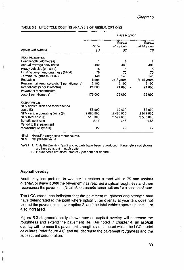
Chapter 5
l
TABLE 5.3 LIFE CYCLE COSTING ANALYSIS OF RESEAL OPTIONS
Inputs and outputs
Reseal option
Reseal Reseal None at 7 years at 14 years
!l) (2) (3)
Input parameters Road length (kilometres) Annual average daily traffic Heavy vehicles (per cent) Existing pavement roughness (NRM) Terminal roughness (NRM) Resealing Routine maintenance costs ($ per kilometre) Reseal cost ($ per kilometre) Pavement reconstruction cost ($ per kilometre)
Output results NPV construction and maintenance
NPV vehicle operating costs ($) NPV total cost ($) Benefit-cost ratio Period to first pavement reconstruction (years)
costs ($1
1 400
18 70 140
None 2 100 21 000
175 000
58 000 2 060 000 2 519 000
2.1 1
22
1 400
18 70 140
At 7 years 2 100 21 000
175 000
62 000 2 465 000 2 527 000
1.48
29
l 400
18 70 140
At 14 years 2 100 21 000
175 000
57 000 2 072 000 2 530 000
1.66
27
NRM NAASRA roughness meter counts. NPV Net present value.
Notes 1. Only the primary inputs and outputs have been reproduced. Parameters not shown are held constant in each option.
2. Future costs are discounted at 7 per cent per annum.
Asphalt overlay
Another typical problem is whether to resheet a road with a 75 mm asphalt overlay, or leave it until the pavement has reached a critical roughness and then reconstruct the pavement. Table 5.4 presents these options for a section of road.
The LCC model has indicated that the pavement roughness and strength may have deteriorated to the point where option 3, an overlay at year ten, does not extend the pavement life over option 2, and the total vehicle operating costs are also increased.
Figure 5.3 diagrammatically shows how an asphalt overlay will decrease the roughness and extend the pavement life. As noted in chapter 4, an asphalt overlay will increase the pavement strength by an amount which the LCC model calculates (refer figure 4.6) and will decrease the pavement roughness and the subsequent deterioration.
39
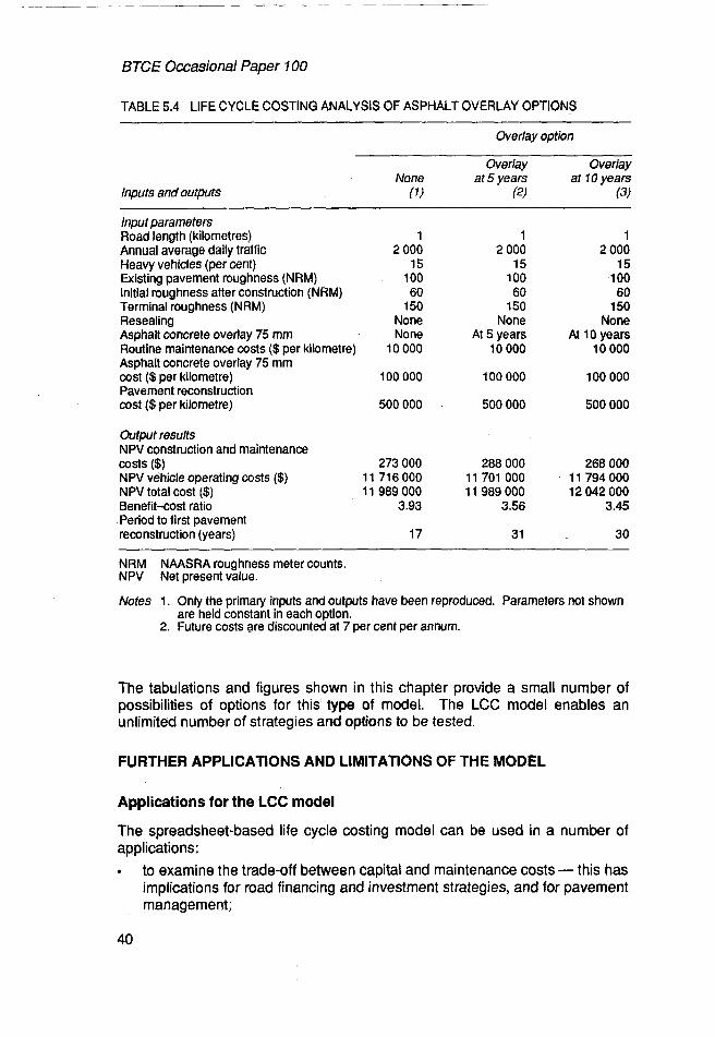
BTCE Occasional Paper 100
TABLE 5.4 LIFE CYCLE COSTING ANALYSIS OF ASPHALT OVERLAY OPTIONS
Overlay option
Overlay Overlay None at 5 years at 10 years
Inputs and outputs (7) (2) (3)
Input parameters Road length (kilometres) Annual average daily traffic Heavy vehicles (per cent) Existing pavement roughness (NRM) Initial roughness after construction (NRM) Terminal roughness (NRM) Resealing Asphalt concrete overlay 75 mm Routine maintenance costs ($ per kilometre) Asphalt concrete overlay 75 mm cost ($ per kilometre) Pavement reconstruction cost ($ per kilometre)
1 2 000
15 100 60 150
None None
10 000
100 000
500 000
1 2 000
15 100 60 150
None At 5 years
10 000
100 000
500 000
1 2 000
15 100 60 150
None At 10 years
l0 000
100 000
500 000
Output results NPV construction and maintenance
NPV vehicle operating costs ($) 1 1 716000 1 1 701 000 11 794 000 NPV total cost ($) 1 1 989 000 1 1 989 000 12 042 000 Benefit-cost ratio 3.93 3.56 3.45 Period to first pavement reconstruction (years) 17 31 30
NRM NAASRA roughness meter counts. NPV Net present value.
Notes 1. Only the primary inputs and outputs have been reproduced. Parameters not shown
costs ($1 273 000 288 000 268 000
are held constant in each option. 2. Future costs are discounted at 7 per cent per annum.
The tabulations and figures shown in this chapter provide a small number of possibilities of options for this type of model. The LCC model enables an unlimited number of strategies and options to be tested.
FURTHER APPLICATIONS AND LIMITATIONS OF THE MODEL
Applications for the LCC model
The spreadsheet-based life cycle costing model can be used in a number of applications:
to examine the trade-off between capital and maintenance costs - this has implications for mad financing and investment strategies, and for pavement management;
40
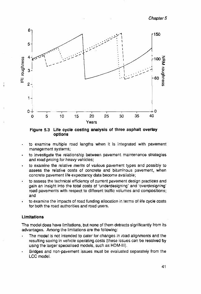
Chapter 5
I
/
/
O l I I I l I I I 10 0 5 10 15 20 25 30 35 40
Years
Figure 5.3 Life cycle costing analysis of three asphalt overlay options
- to examine multiple road lengths when it is integrated with pavement management systems; to investigate the relationship between pavement maintenance strategies and road pricing for heavy vehicles: to examine the relative merits of various pavement types and possibly to assess the relative costs of concrete and bituminous pavement, when concrete pavement life expectancy data become available; to assess the technical efficiency of current pavement design practices and gain an insight into the total costs of ‘underdesigning’ and ‘overdesigning’ road pavements with respect to different traffic volumes and compositions; and to examine the impacts of road funding allocation in terms of life cycle costs for both the road authorities and road users.
Limitations
The model does have limitations, but none of them detracts significantly from its advantages. Among the limitations are the following:
The model is not intended to cater for changes in road alignments and the resulting saving in vehicle operating costs (these issues can be resolved by using the larger specialised models, such as HDM-Ill).
. Bridges and non-pavement issues must be evaluated separately from the LCC model.
41

BTCE Occasional Paper 100
The results of the model, as is the case with all similar models, are only as accurate as the mathematical relationships used. However, these relationships, and hence the accuracy of the model, can be continually improved as data become available. The model was not designed for rigid or unsealed pavements. It can, however, act as a framework for incorporating these pavements as data become available.
42
It is important that pavement construction and maintenance decisions are based on the best available information. With its simplicity and comparatively small data requirements, the life cycle costing model can provide engineers and decision-makers with a valuable tool for better allocating road funds, and road construction and maintenance strategies. The model is flexible enough to allow modification to data inputs so as to accommodate different pavement configurations and local environments. The model will provide a framework for subsequent research on this subject.
The Bureau’s work and the life cycle costing model are steps towards understanding pavement deterioration. The model will provide an economic and engineering tool for examining road pavements, their use, and reconstruction and maintenance options.
43

APPENDIX I DEFLECTIONS AND STRUCTURAL NUMBERS FOR NEW PAVEMENTS
For existing pavements, the structural number, which is required as input to the life cycle costing model, can be measured. For new pavements, the structural number needs to be calculated. This appendix provides examples of the results of such calculations, based on NAASRA (1 987b), for pavement depth, pavement deflection and pavement structural number for a thin bituminous surfacing (flush seal) on an unbound 500, 350 or 250 megapascal base comprised of crushed rock or gravel.
The thickness T in each table is the design thickness, computed using NAASRA (1987b). The pavement thicknesses T - 30 per cent and T - 15 per cent represent pavements thinner than the NAASRA design, and T + 15 per cent and T + 30 per cent represent thicker pavements. These have been included as a first step in assessing the cost-effectiveness of differing pavement designs.
The structural numbers shown in tables 1.3,1.5 and 1.7 have been computed using the surface deflections shown in tables 1.2, 1.4 and 1.6. The ELSYM5 computer program has been used.
45
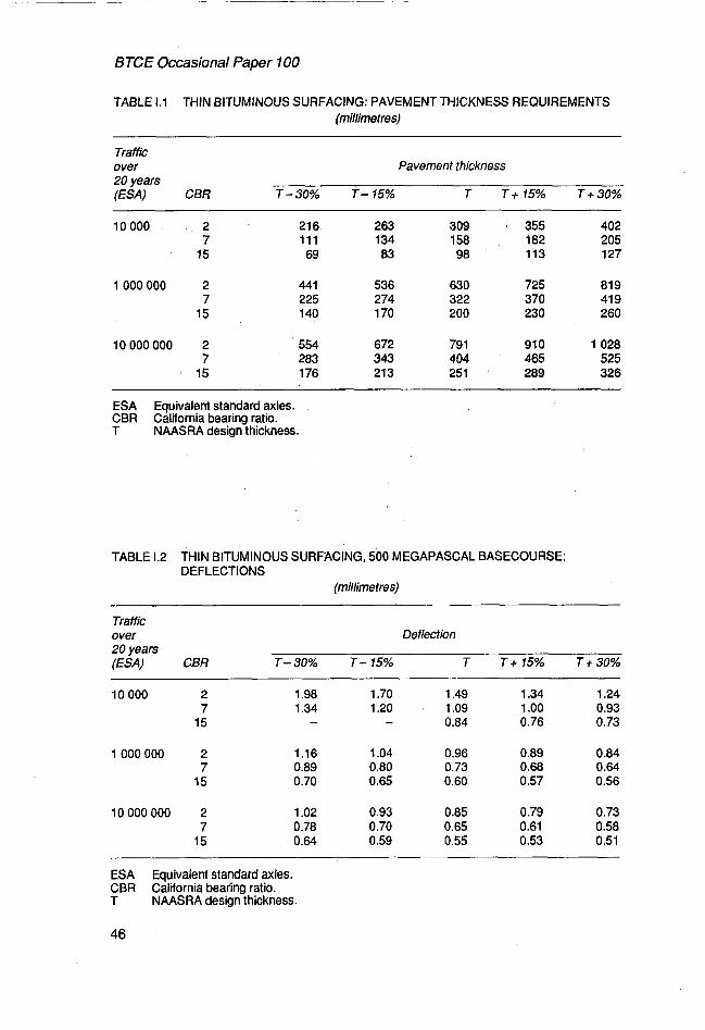
BTCE Occasional Paper 100
TABLE 1.1 THIN BITUMINOUS SURFACING: PAVEMENT THICKNESS REQUIREMENTS (millimetres)
~~
Traffic over Pavement thickness 20 years ( E W CBR T - 3 0 % T - 15% T T + 1 5 % T + 3 0 %
10 000 2 21 6 263 309 355 402 7 111 134 158 182 205
15 69 83 98 113 127
l 000 000 2 441 536 630 725 81 9 7 225 274 322 370 41 9
15 140 1 70 200 230 260
10000000 2 554' 672 791 91 0 1 028 7 283 343 404 . 465 525
' 15 176 213 25 1 289 326
ESA Equivalent standard axles. CBR California bearing ratio. T NAASRA design thickness.
TABLE 1.2 THIN BITUMINOUS SURFACING, 500 MEGAPASCAL BASECOURSE: DEFLECTIONS
(millimetres)
Traffic over Deflection 20 years ( E W CBR T - 3 0 % T - 15% T T + 15% T + 3 0 %
10 000 2 1.98 1.70 1.49 1.34 1.24 7 1.34 1.20 1.09 1 .oo 0.93
- - 0.84 0.76 0.73 15
1 000 000 2 1 . l6 1.04 0.96 0.89 0.84 7 0.89 0.80 0.73 0.68 0.64
15 0.70 0.65 0.60 0.57 0.56
10 000 000 2 1.02 0.93 0.85 0.79 0.73 7 0.78 0.70 0.65 0.61 0.58
15 0.64 0.59 0.55 0.53 0.51
ESA Equivalent standard axles. CBR California bearing ratio. T NAASRA design thickness.
46
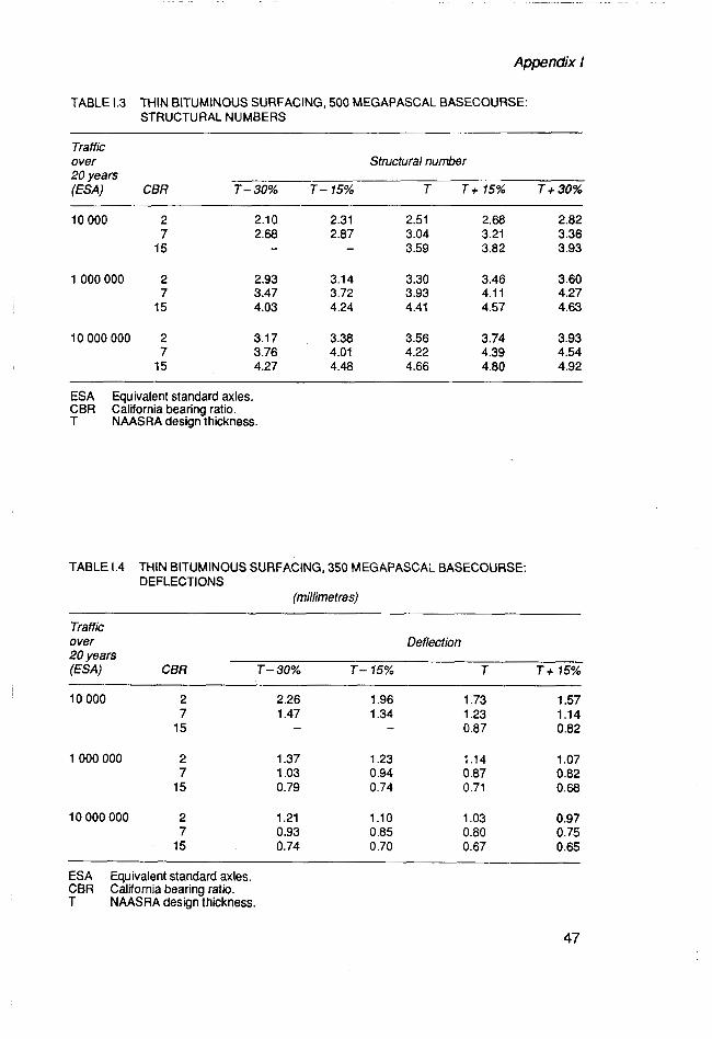
Appendix I
TABLE 1.3 THIN BITUMINOUS SURFACING, 500 MEGAPASCAL BASECOURSE: STRUCTURAL NUMBERS
Traffic over Structural number 20 years ( E W CBR T-30% T- 15% T T + 15% T+30%
10 000 2 7 15
1 000 000 2 7 15
10 000 000 2 7 15
2.10 2.68
2.93 3.47 4.03
3.1 7 3.76 4.27
2.31 2.87
3.14 3.72 4.24
3.38 4.01 4.48
2.51 3.04 3.59
3.30 3.93 4.41
3.56 4.22 4.66
2.68 3.21 3.82
3.46 4.1 1 4.57
3.74 4.39 4.80
2.82 3.36 3.93
3.60 4.27 4.63
3.93 4.54 4.92
ESA Equivalent standard axles. CBR California bearing ratio. T NAASRA design thickness.
TABLE 1.4 THIN BITUMINOUS SURFACING, 350 MEGAPASCAL BASECOURSE: DEFLECTIONS
(millimetres)
Traffic over Deflection 20 years ( E W CBI? T - 30% T- 15% T J+ 75%
10 000 2 2.26 1.96 1.73 1.57 7 1.47 1.34 1.23 1 .l4
- 0.87 0.82
~
15 -
1 000 000 2 1.37 1.23 1 .l4 1.07 7 1.03 0.94 0.87 0.82 15 0.79 0.74 0.71 0.68
10 000 000 2 1.21 1 .l0 l .03 0.97 7 0.93 0.85 0.80 0.75 15 0.74 0.70 0.67 0.65
ESA Equivalent standard axles. CBR California bearing ratio. T NAASRA design thickness.
47
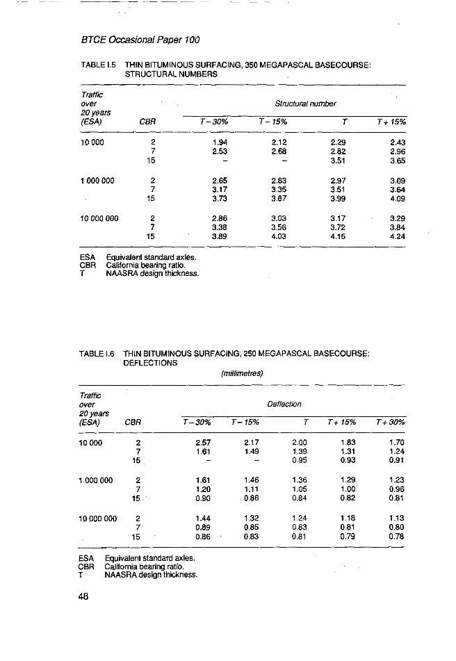
BTCE Occasional Paper 700
TABLE 1.5 THIN BITUMINOUS SURFACING, 350 MEGAPASCAL BASECOURSE: STRUCTURAL NUMBERS
Traffic over Structural number 20 years ( E W CBR T- 30% T- 15% T T+ 15%
10 000 2 1.94 2.12 2.29 2.43 7 2.53 2.68 2.82 2.96
- - 3.51 3.65 15
1 000 000 2 2.65 2.83 2.97 3.09 7 3.17 3.35 3.51 3.64 15 3.73 3.87 3.99 4.09
10 000 000 2 2.86 3.03 3.17 3.29 7 3.38 3.56 3.72 3.84 15 3.89 4.03 4.15 4.24
ESA Equivalent standard axles. CBR California bearing ratio. T NAASRA design thickness.
TABLE 1.6 THIN BITUMINOUS SURFACING, 250 MEGAPASCAL BASECOURSE: DEFLECTIONS
(millimetres)
Traffic over Deflection 20 years ( E W CBR T - 30% T- 15% T T + 75% T+30%
~~
10 000 2 2.57 2.17 2.00 1.83 1.70 7 1.61 1.49 1.39 1.31 1.24
- - 0.95 0.93 0.91 15
1 000 000 2 1.61 1.46 1.36 1.29 1.23 7 1.20 1.11 1.05 1 .oo 0.96 15 0.90 0.86 0.84 0.82 0.81
10000 000 2 1.44 l .32 1.24 1 .l8 1 .l3 7 0.89 0.85 0.83 0.81 0.80 15 0.86 0.83 0.81 0.79 0.78
ESA Equivalent standard axles. CBR California bearing ratio. T NAASRA design thickness.
48
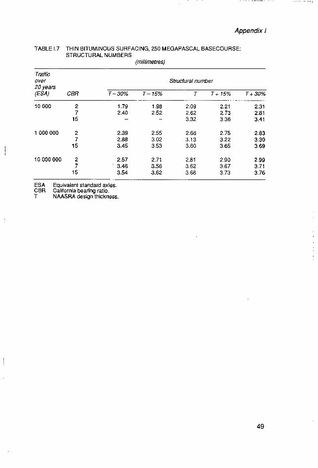
Appendix I
TABLE 1.7 THIN BITUMINOUS SURFACING, 250 MEGAPASCAL BASECOURSE: STRUCTURAL NUMBERS
(millimetres)
Traffic over Structural number 20 years (=A) CBR T-30% T - 15% T T + 75% T+30%
10 000 2 7 15
1 000 000 2 7
l 15
10000000 2 7 15
1.79 2.40
-
2.39 2.88 3.45
2.57 3.46 3.54
1.98 2.52
-
2.55 3.02 3.53
2.71 3.56 3.62
2.09 2.62 3.32
2.66 3.13 3.60
2.81 3.62 3.68
2.21 2.73 3.36
2.75 3.22 3.65
2.90 3.67 3.73
2.31 2.81 3.41
2.83 3.30 3.69
2.99 3.71 3.76
ESA Equivalent standard axles. CBR California bearing ratio. T NAASRA design thickness.
49
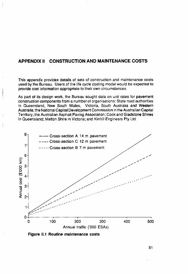
APPENDIX II CONSTRUCTION AND MAINTENANCE COSTS
This appendix provides details of sets of construction and maintenance costs used by the Bureau. Users of the life cycle costing model would be expected to provide cost information appropriate to their own circumstances.
As part of its design work, the Bureau sought data on unit rates for pavement construction components from a number of organisations: State road authorities in Queensland, New South Wales, Victoria, South Australia and Western Australia; the National Capital Development Commission in the Australian Capital Territory; the Australian Asphalt Paving Association; Cook and Gladstone Shires in Queensland; Melton Shire in Victoria; and Kinhill Engineers Pty Ltd.
Cross-section A 14 m pavement "" Cross-section C 12 m pavement ...... Cross-section B 7 m pavement
Annual traffic ('000 ESAs)
Figure 11.1 Routine maintenance costs
51

BTCE Occasional Paper 100
The data were tabulated and averaged to produce typical 1988 unit rates which were then used for each of the representative cross-sections (A, B and C), as shown in figure 4.1, to produce cost per kilometre rates, as set out in tables 11.1, 11.2 and 11.3. These tables cover the following types of pavements:
type I -flush seals on an unbound base; . type II - 50-millimetre asphalt concrete; and
type I l l - 100-millimetre asphalt concrete on an unbound base.
The Bureau also sought from the same sources information about typical maintenance costs; the data supplied were, however difficult to compare or average. Maintenance expenditure is evidently much more variable than construction costs, and it has been assumed to be related to traffic conditions.
On the basis of the limited data received and the experience of those involved in the project, the Bureau synthesised a routine maintenance cost per annum from the annual traffic rates. This is included as figure 11.1.
Finally, reseal and shape correction maintenance activities were costed on the basis of construction rates after due allowance for the smaller scale of the works. Rates per kilometre are listed in table 11.4.
This information is provided for guidance only.
52
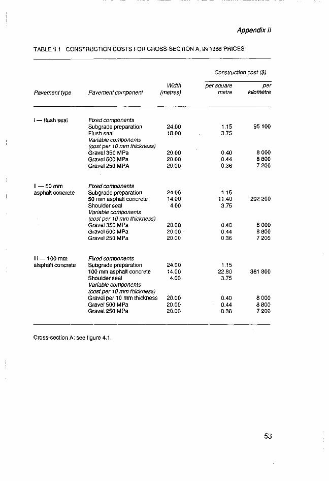
Appendix II
TABLE 11.1 CONSTRUCTION COSTS FOR CROSS-SECTION A, IN 1988 PRICES
Construction cost ($)
Width per square Per Pavement type Pavement component (metres) metre kilometre
I -flush seal fixed componenfs Subgrade preparation Flush seal Variable components (cost per 70 mm thickness) Gravel 350 MPa Gravel 500 MPa Gravel 250 MPA
II -50 mm Fixed components asphalt concrete Subgrade preparation
50 mm asphalt concrete Shoulder seal Variable components (cost per IO mm thickness) Gravel 350 MPa Gravel 500 MPa Gravel 250 MPa
111 - 100 mm Fixed components alsphalt concrete Subgrade preparation
100 mm asphaR concrete Shoulder seal Variable components (cost per 70 mm thickness) Gravel per 10 mm thickness Gravel 500 MPa Gravel 250 MPa
24.00 18.00
20.00 20.00 20.00
24.00 14.00 4.00
20.00 20.00 20.00
24.00 14.00 4.00
20.00 20.00 20.00
1.15 95 100 3.75
0.40 8 000 0.44 8 800 0.36 7 200
1 .l5
3.75 11.40 202 200
0.40 8 000 0.44 8 800 0.36 7 200
1 .l5
3.75 22.80 361 800
0.40 8 000 0.44 8 800 0.36 7 200
Cross-section A: see figure 4.1.
53
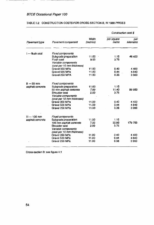
BTCE Occasional Paper 100
TABLE 11.2 CONSTRUCTION COSTS FOR CROSS-SECTION B, IN 1988 PRICES
Construction cost $
Width per square Per Pavement type Pavement component (metres) metre kilometre
I -flush seal
II - 50 mm asphalt concrete
111 - 100 mm asphalt concrete
Fixed components Subgrade preparation Flush seal Variable components (cost per 10 mm thickness) Gravel 350 MPa Gravel 500 MPa Gravel 250 MPA
Fixed components Subgrade preparation 50 mm asphalt concrete Shoulder seal Variable components (cost per 10 mm thickness) Gravel 350 MPa Gravel 500 MPa Gravel 250 MPa
Fixed components Subgrade preparation l00 mm asphalt concrete Shoulder seal Variable components (cost per 7 0 mm thickness) Gravel 350 MPa Gravel 500 MPa Gravel 250 MPa
l l .oo 9.00
1 1 .oo 1 1 .oo 1 1 .oo
1 1 .oo 7.00 2.00
11 .oo l 1 .oo 11 .oo-
1 1 .oo 7.00 2.00
1 1 .oo 1 1 .oo 1 1 .oo
1.15 3.75
0.40 0.44 0.36
l .l5 1 1.40 3.75
0.40 0.44 0.36
1.15 22.80 3.75
0.40 0.44 0.36
46 400
4 400 4 840 3 960
99 950
4 400 4 840 3 960
179 750
4 400 4 840 3 960
Cross-section B: see figure 4.1
54

Appendix II
TABLE 11.3 CONSTRUCTION COSTS FOR CROSS-SECTION C, IN 1988 PRICES
Construction cost $
Width per square Pavement type Pavement component (metres) metre
I -flush seal Fixed components Subgrade preparation 12.80 1 .l5 Flush seal 12.80 3.75 Variable components (cost per 10 mm thickness) Gravel 350 MPa 12.80 0.40 Gravel 500 MPa 12.80 0.44 Gravel 250 MPA 12.80 0.36
I I -50 mm Fixed components asphalt concrete Subgrade preparation 12.80 1 .l5
50 mm asphalt concrete 12.80 11.40 Variable components (cost per 10 mm thickness) Gravel 350 MPa 12.80 0.40 Gravel 500 MPa 12.80 0.44 Gravel 250 MPa 12.80 0.36
111 - 100 mm Fixed wmponents asphalt concrete Subgrade preparation 12.80 1.15
100 mm asphalt concrete 12.80 22.80 Variable components (cost per 10 mm thickness) Gravel 350 MPa 12.80 0.40 Gravel 500 MPa 12.80 0.44 Gravel 250 MPa 12.80 0.36
Per kilometre
62 720
5 120 5 632 4 608
160 640
5 120 5 632 4 608
306 560
5 120 5 632 4 608
Cross-section C: see figure 4.1,
55
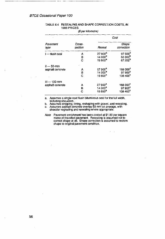
BTCE Occasional Paper 700
TABLE 11.4 RESEALING AND SHAPE CORRECTION COSTS, IN 1988 PRICES
($ per kilometre)
cost
Pavement CrOSS- Shape type section Reseal correction
~~~~ ~
I -flush seal A B C
II - 50-mm asphalt concrete A
B C
111 - 100-mm asphalt concrete A
B C
27 900a 14 OOOa 19 800a
27 900a 14 OOOa 19 800a
27 900a 14 OOOa 19 800a
97 500b 50 300b 67 200b
188 000'
138 400' 97 gooc
188 000'
138 400' 97 gooc
a. Assumes a single coat flush bituminous seal for the full width,
b. Assumes stripping, tining, reshaping with gravel, and resealing. c. Assumes asphalt concrete overlay 50 mm on average, with
Note Pavement enrichment has been costed at $1 .OO per square metre of travelled pavement. Resealing is assumed not to correct shape at all. Shape correction is assumed to restore shape to original pavement condition.
including shoulders.
shoulder regrading and resealing where appropriate.
56
REFERENCES
Anderson, D. (1989), Pavement Management in Victoria, Implementation of a System to Assist the Road Construction Authority, in 45th Municipal Engineers Conference (Vic.), Local Government Engineers Association of Victoria & Road Construction Authority, Melbourne.
Australian Road Research Board (1 989), NAASRA Roughness Meter Calibration via the Road-profile-based International Roughness index (/RI), Research Report ARR 164, Australian Road Research Board, Melbourne.
AUSTROADS (1 989), Pavement Management in Australia - National Issues, AUSTROADS, Sydney.
Blanchard, B. S. (1978), Design and Manage to Life Cycle Cost, M/A Press, Oregon.
- (1 986), Logistics Engineering and Management, Prentice-Hall, Englewood Cliffs, New Jersey.
Blanchard, B. S. & Fabrysky, W. J. (1981), System Engineering and Analysis, Prentice-Hall, Englewood Cliffs, New Jersey.
BTCE (1 987), Assessment of the Australian Road System: 1987, Report 61, AGPS, Canberra.
- (1 989), Australian Road Financing Statistics, 1977-78 to 1986-87, Information Paper 33, AGPS, Canberra.
Calvert, F. (1 986), Development of the Federal Bureau of Transport Economics Pavement Life Cycle Costs Model, paper presented at 8th Conference of Australian Institutes of Transport Research, Launceston.
Cox, J. B. & Rolt, J. (1986), An Integrated Approach to Pavement Design Based on HDM-Ill, in Proceedings 13th ARRB Conference, vol. 13, part 4, Australian Road Research Board, Melbourne, pp. 135-49.
Department of Finance (1 987), The Choice ofDiscountRate forEvaluating Public Sector Investment Projects - Discussion Paper, Department of Finance, Canberra.
57
BTCE Occasional Paper 100
Department of Transport and Works, Northern Territory (1 989), Victoria Highway Development Strategy - Pavement Life Prediction, Department of Transport and Works, Darwin.
Gutteridge, Haskins i3 Davey (1 986), Road Renewal and Maintenance Strategy Model, Mackay City Council, Mackay, Queensland.
Hill, P., Youdale, G. P., Mallon, P., Sheldon, G. N., Haley, M., Bagia, R. K., Lowe, O., Campbell, N., Glanville, D., Kirbos, E. and Hibberd, S. (1988), Deflectolab - Truck Mounted Automated Pavement Deflection Measuring Device, in Proceedings 14th ARRB Conference, vol. 5, Australian Road Research Board, Melbourne.
Hoban, C. (1988), The Highway Design and Maintenance Model HDM-Ill - an Introduction, in Proceedings of the Workshop on the Highway Design and Maintenance Model HDM-Ill, Australian Road Research Board, Melbourne.
Hollingworth, C. & O’Brien, B. E. (1988), CHIMP - a Powerful Microcomputer Asset Management System for Road Authorities, in Proceedings 74th ARRB Conference, vol. 5, Australian Road -Research Board, Melbourne.
Jameson, G. W., Baran, B. T. & Sheldon, G. N. (1988), Australian Experience with the Swedish Laser Road Surface Tester, in Proceedings 14th ARRB Conference, vol. 5, Melbourne.
Lay, M. G. (1986), Handbook of Road Technology, vol. 8, Planning and Pavements, Gordon and Breach Science, New York.
Loong, K. Y. i3 Miller, J. E. (1 989), Road Pavement Design and Maintenance - A Life Cycle Cost Approach, in lnternationalConference Proceedings ‘Transpo’89, Ministry of Communications, Beijing, China.
NAASRA (1 987a), A Guide to the Visual Assessment of Pavement Condition, NAASRA, Sydney.
- (1987b), Pavement Design - Guide to the Structural Design of Road Pavements, NAASRA, Sydney.
NCHRP (1 985), Life-cycle CostAnalysis ofpavements Transportation Research Board, National Research Council, Washington D.C.
NRMA (1989), What it Costs to Run Your Car, NRMA, Sydney.
Parsley, L. i3 Robinson, R. (1982). The TRRL Road Investment Model for Developing Countries (RTI”), Laboratory Report 1057, Transport and Road Research Laboratory, Crowthorne, England.
Paterson, W. D. 0. (1986), Prediction of Road Deterioration, in Proceedings 73th ARRB Conference, vol. 13, part 4, Australian Road Research Board, Melbourne.
References
- (1 987), Road Det erioration and Mainte nan ce Effects - Models for Planning and Management, Johns Hopkins University Press, Baltimore.
Potter, D. W. & Hudson, W. R. (1981), Optimisation of Highway Maintenance Using Highway Design Model, Australian Road Research, 11 (1).
Powell, D. W., Potter, J. F., Mayhew, H. C. & Nunn, M. E. (1 984), The Structural Design of Bitumen Roads, Laboratory Report 1132, Transport and Road Research Laboratory, Crowthorne, England.
Roads and Traffic Authority (1 989), Simplified Cost Benefit Analysis, unpublished report, Road and Traffic Authority, New South Wales, Sydney, July.
Satish, C. & Lingras, P. J. (1989), Cost of Driving and Convenience for Two-lane Highways, Journal of Transportation Engineering, 1 15:no. 3, May.
Uddin, W., Carmichael, R. F. & Hudson, W. R. (1986), Life Cycle Analysis of Pavement Management Decision Making -Final Report, Department of Transportation, Washington, D.C.
Ullidtz, P. (1983), Paper presented at Transportation Research Board Meeting, Washington D.C. January.
Watanatada, T., Dhareswar, A. M. & Rzende-Lima, P. R. S. (1985), Models for Predicting Vehicle Speeds and Operating Costs based on Mechanistic Principles, in Highway Design and Maintenance Standards Study, World Bank, Washington, D.C.
Watanatada, T., Harral, C. G., Paterson, W. D. O., Dhareshwar, A. M., Bhandari, A. & Tsunokawa, K. (1 987), The Highway Design and Maintenance Standards Model, vols 1 & 2, Johns Hopkins University Press, Baltimore.
Wheatstone, S., Gargett, D., Ada, N. & Noon, M. (1 988), Roadsim: An Economic Simulation Model of the Australian Road System, in Proceedings 14th ARRB Conference, vol. 14, Australian Road Research Board, Melbourne, Canberra, pp. 236-46.
World Bank(1986), The Highway Design and Maintenance Standards Model, vol. 1, Description of the HDM-Ill Model, World Bank, Washington, D.C.
- (1987), Vehicle Operating Costs: Users Manual, World Bank, Washington, D.C.
- (1988), Road Transport Taxation in Developing Countries, Discussion Paper 26, World Bank, Washington, D.C.
59
ABBREVIATIONS
AADT BTCE CBR CHIMP
CIRCLY ELSYM5 €SA HDM-Ill IRI LCC NAASRA NCHRP NIMPAC NPV NRM NRMA PMS PS I REVS ROADSIM SIMCBA SOC SRTP VOC
Annual average daily traffic Bureau of Transport and Communications Economics California bearing ratio Construction History Inventory and Miscellaneous Records Program A computer based pavement design program A computer based pavement design program Equivalent standard axle Highway Design and Maintenance Standards Model International roughness index Life cycle costing National Association of Australian State Road Authorities National Co-operative Highway Research Program NAASRA Improved Model for Project Assessment Costing Net present value NAASRA Roughness Meter National Roads and Motorists’ Association Pavement management system Pavement serviceability index Road evaluation system Road Simulation Model of the Australian Road System Simplified Cost Benefit Analysis Social opportunity cost of capital Social rate of time preference Vehicle operating costs
61