road traﬃc noise prediction model ‘‘asj rtn-model 2018

Road traffic noise prediction model ‘‘ASJ RTN-Model 2018’’:

Report of the Research Committee on Road Traffic Noise

Shinichi Sakamoto

Chairman of the Research Committee on Road Traffic Noise, Acoustical Society of Japan

Keywords: Road traffic noise, Prediction model, Sound power level, Sound propagation, Predictionaccuracy

PACS number: 43.50.Lj, 43.28.Js [doi:10.1250/ast.41.529]

PREFACE

Background

In 1974, the Acoustical Society of Japan first organized

a research committee to develop a road traffic noise

prediction model. This committee has been continuously

undertaking research activities since then with the aim of

developing an adequate prediction method for road traffic

noise on the basis of state-of-the-art knowledge in response

to the demands of trends [1]. As a result of its activities, a

prediction model called ASJ Model 1975 was published

in 1975, which provided a method of calculating the 50

percentile A-weighted sound pressure level (LA50) [2,3].

This model was widely accepted and applied to assess-

ments of noise around roads for many years. After that,

research activities were continued to improve the accuracy

of prediction and expand the scope of its application [4–6].

In parallel with these activities, from 1988, the committee

worked on the development of a new prediction method

based on the equivalent continuous A-weighted sound

pressure level (LAeq). The outcomes of the research were

summarized, and the calculation model (ASJ Model 1993)

was published in 1994 [7]. This model proposed general

procedures for the calculation of LAeq at roads with a

uniform cross-sectional structure.

Afterwards, there was a substantial change in the

environmental administration concerning noise. In June

1997, the ‘‘Environmental Impact Assessment Law’’ was

promulgated, whose enactment was based on the ‘‘Environ-

ment Basic Law’’ (the law revising the ‘‘Basic Law for

Environmental Pollution Control,’’ which was issued in

November 1993), and it was enforced in June 1999, two

years after its promulgation. In addition, the ‘‘Environ-

mental Quality Standards for Noise’’ (enacted in 1971) was

revised in September 1998 and enforced in April of the

following year. In the standards, LAeq was adopted in place

of LA50 as the noise index for road traffic assessment. At the

same time, the standard values for general residential areas

and areas facing roads were renewed.

Corresponding to these changes, the above-mentioned

ASJ Model 1993 was later developed further on the basis of

a surveillance study, and ASJ Model 1998 was reported in

April 1999 as a new model based on LAeq assessment [8].

The model had an expanded scope of application to cover

almost all types of roads and structures, including general

roads and special road sections, such as interchanges, road

tunnels, semi-underground roads, and overhead/double-

deck viaducts. In addition, the structure-borne noise of

viaduct roads was newly included in this model. Shortly

after its report, further research activity was started with

the aims of expanding its field of application, introducing

wave-based computational methods for sound propagation,

and improving the prediction accuracy. As a result, ASJ

RTN-Model 2003 [9], ASJ RTN-Model 2008 [10], and ASJ

RTN-Model 2013 [11] were completed and published in

April 2004, April 2009, and April 2014, respectively.

ASJ Model 1998 and newer models were comprehen-

sively adopted in the ‘‘Technical Method for Environ-

mental Impact Assessment of Roads’’ and have been

widely used for road traffic noise prediction (the assess-

ment of future environments) in Japan [12,13]. The ASJ

RTN-Model is also used to design environmental preser-

vation measures (noise abatement measures) and to

estimate the current state of noise during environmental

monitoring (regular observation). Thus, on the basis of the

fact that the prediction model is used for not only the

prediction of future environments but also the estimations

of present environments and the design of noise mitigation

measures, the research committee has been working on

finding solutions to the problems remaining unsolved in

ASJ RTN-Model 2013 [14]. After five years of research

and investigation, the new model, ‘‘ASJ RTN-Model

2018,’’ has been completed and is published in this Journal.

529

Acoust. Sci. & Tech. 41, 3 (2020) #2020 The Acoustical Society of Japan

INVITED REVIEW

http://dx.doi.org/10.1250/ast.41.529

Table 1.1 shows the organization and the members of

the committee. In this report, the results of research and

investigation are summarized.

Summary of the revisions in the current version

The contents of ASJ RTN-Model 2018 are shown in

Table 1.2. The current model is based on ASJ RTN-Model

2013 to which the following revisions were made.

(1) Sound source characteristics

. The classification of road vehicles from an acoustical

viewpoint was reviewed and changed from the

conventional four-category classification to a three-

category classification.

. The values of the A-weighted sound power level of

road vehicles were updated, and their calculation

methods were given for respective types of road

pavement.

. In the types of road pavement, a gap-graded asphalt

mixture (referred to as ‘‘KOUKINOU II’’) was newly

included.

. The representative sound power spectra of vehicle

noise, which are shown in Appendix A1, are revised

usign the latest data.

. The latest knowledge on the A-weighted sound power

levels of hybrid vehicles (HVs) and electric vehicles

(EVs) is shown in Appendix A2.

. Sound power levels on dense asphalt in an accelerat-

ing traffic flow section are shown in Appendix A3.

Sound power levels on general roads paved with

porous asphalt are shown in Appendix A4.

(2) Calculation of sound propagation

. The corrections due to sound attenuation by diffrac-

tion and reflection were reviewed, and part of calcula-

tion formulae and values of coefficients were updated.

. For correction for diffraction, sound diffraction over a

knife wedge (assuming a barrier) and that over a right-

angled wedge (assuming an embankment or a build-

ing) were discriminated, and formulae for respective

fundamental correction terms were given.

. According to the update of sound power spectra of

vehicles and the addition of KOUKINOU II to road

pavement types, values of the coefficients for calcu-

lation formulae for correction terms for diffraction

were updated.

. The calculation methods for a thick barrier and a

barrier with an overhung were changed.

Table 1.1 Organization and members of the research committee on road traffic noise.

Name Affiliation

Chair Shinichi Sakamoto Institute of Industrial Science, The University of Tokyo

Secretaries Ken Anai Faculty of Engineering, Fukuoka University

Yasuaki Okada Faculty of Science and Technology, Meijo University

Akinori Fukushima NEWS Environmental Design Inc.

Toshio Matsumoto Kobayasi Institute of Physical Research

Yosuke Yasuda Faculty of Engineering, Kanagawa University

Katsuya Yamauchi Faculty of Design, Kyushu University

Takatoshi Yokota Kobayasi Institute of Physical Research

Members Ryuji Inoue�1 National Institute for Land and Infrastructure Management

Akiyoshi Ito Japan Automobile Research Institute

Hiroyuki Imaizumi National Institute of Advanced Industrial Science and Technology

Terutoshi Tajika Environmental Technical Laboratory, Ltd.

Kunio Nakasaki�1 Nippon Expressway Research Institute Co., Ltd.

Osamu Funahashi�2 Nippon Expressway Research Institute Co., Ltd.

Toshiaki Mabuchi�2 National Institute for Land and Infrastructure Management

Technical adviser Hideo Ohno Hino Motors, Ltd.

Advisers Teruo Iwase Professor Emeritus at Niigata University

Yasuo Oshino Former Senior Chief at Japan Automobile Research Institute

Kazutoshi Fujimoto Professor Emeritus at Kyushu University

Kohei Yamamoto Kobayasi Institute of Physical Research

�1Until fiscal 2017, �2From fiscal 2018

Acoust. Sci. & Tech. 41, 3 (2020)

530

. The calculation method for the ground effect over a

porous asphalt pavement was newly added.

. For the scattered reflection method included in the

calculation method of sound reflection, the method of

setting the calculation conditions was described.

. On the basis of the numerical investigation of the

meteorological effect on the sound propagation of

road traffic noise, the upper limit of attenuation effect

due to diffraction and the ground effect was deter-

mined.

. The calculation method of frequency-dependent prop-

agation was updated to the generalized energy-baseed

method. The method is shown in Appendix A5.

. For a calculation method based on the wave-based

numerical analyses, the contents are updated. The

details are shown in Appendix A6.

(3) Special road sections

. The calculation method of noise around a road tunnel

was changed to a method taking into consideration

directivity characteristics of sound radiation from the

tunnel mouth.

. For noise around flat/overhead roads and double-deck

viaducts, the calculation method of scattered reflec-

tion was simplified.

. The calculation method of noise prediction at signal-

ized intersections was updated. The details are shown

in Appendix A7.

(4) Noise behind a single building and in built-up areas

. For road traffic noise in built-up areas, the calculation

method based on a point source model given in the

previous model was simplified from an engineering

viewpoint and the content was updated.

. The detailed calculation method based on a point

Table 1.2 Contents of ASJ RTN-Model 2018.

Chapter Section

1. Outline of the prediction method 1.1 Scope(general procedure) 1.2 Terms and definitions

1.3 General calculation procedure and basic equations

2. Sound source characteristics 2.1 Classification of road vehicles2.2 Sound power levels of road vehicles2.3 Correction of sound power level for various factors

3. Method of calculating sound 3.1 Basic equationspropagation 3.2 Correction for diffraction �Ldif

3.3 Correction for ground effect �Lgrnd

3.4 Correction for atmospheric absorption �Lair

3.5 Calculation of sound reflection3.6 Meteorological effect

4. Noise at special road sections 4.1 Interchanges4.2 Junctions4.3 Signalized intersections4.4 Road tunnels4.5 Depressed and semi-underground roads4.6 Flat roads with an overhead viaduct, double-deck viaducts

5. Structure-borne noise of 5.1 Scopeviaducts 5.2 Noise calculation procedure

6. Noise behind single building 6.1 Noise behind single buildingand in built-up areas 6.2 Noise behind building complex

Appendices Appendix A1 Sound power spectra of vehicle noiseAppendix A2 Sound power levels of hybrid and electric vehiclesAppendix A3 Sound power levels of road vehicles on dense asphalt pavement in accelerationAppendix A4 Sound power levels of road vehicles on porous asphalt general roadsAppendix A5 Calculation of frequency-dependent propagationAppendix A6 Wave-based numerical analysisAppendix A7 Signalized intersectionsAppendix A8 Advanced calculation method for noise behind building complex

References Reference R1 Noise reduction effect of double-layer porous asphalt pavementReference R2 Sound propagation around barriers with overhangs and edge-modified barriersReference R3 Expressions for LAeq under simple road conditionsReference R4 Study of prediction accuracy

S. SAKAMOTO: ROAD TRAFFIC NOISE PREDICTION MODEL ‘‘ASJ RTN-Model 2018’’

531

source model is described in Appendix A8.

(5) Others

. Regarding the prediction accuracy of ASJ RTN-

Model 2018, the examinations based on latest knowl-

edge are shown in Reference R4.

ACKNOWLEDGEMENTS

On the occasion of the release of the new prediction

model, the committee would like to express its sincere

thanks to Nippon Expressway Research Institute Co., Ltd.,

who provided opportunities to conduct research activities

concerning road traffic noise, financially supported our

research project, and contributed valuable documents. The

committee would like to express its thanks to the Ministry

of the Environment, Nagoya Expressway Public Corpo-

ration, and Tokyo Metropolitan Government, for their

contribution in providing valuable data. The committee

would also like to thank the National Institute for Land and

Infrastructure Management, Metropolitan Expressway

Co., Ltd., and Hanshin Expressway Co., Ltd., for their

participation in our meetings and for their valuable

suggestions.

MAIN BODY

1. OUTLINE OF THE PREDICTIONMETHOD (GENERAL PROCEDURE)

In this chapter, the scope of ASJ RTN-Model 2018, the

definition or interpretation of technical terms used in this

model, the concept of the calculation method, and the

general procedure of calculation are described.

1.1. Scope

The conditions applicable to ASJ RTN-Model 2018 are

as follows. For conditions related to the structure-borne

noise of viaducts, refer to Chapter 5.

(1) Types of road

General roads (flat, bank, cut, and viaduct) and special

road sections (interchanges, junctions, signalized intersec-

tions, road tunnels, depressed/semi-underground roads, flat

roads with overhead viaducts, and double-deck viaducts).

(2) Traffic volume

No limitation.

(3) Running speed of vehicles

40 to 140 km/h for sections of a steady traffic flow on

expressways and general roads, 0 to 60 km/h for sections

of non-steady traffic flow on general roads, 0 to 80 km/h

for acceleration/deceleration sections on expressways such

as interchanges, 0 to 60 km/h for acceleration/deceleration

sections on general roads, such as in the vicinity of

signalized intersections.

(4) Prediction range

Up to a horizontal distance of 200 m from the road

under consideration and up to a height of 12 m above the

ground.

Note: The validity of the model has been examined for thisprediction range; however, the model is applicable without anylimitation on the calculation range.

(5) Meteorological conditions

No wind or strong temperature profile is assumed as the

standard condition.

1.2. Terms and Definitions

The meanings of the main terms related to the road

traffic noise used in ASJ RTN-Model 2018 are as follows.

(1) A-weighted sound pressure level (LA)

LA is ten times the logarithm to base 10 of the ratio of

the square of the A-weighted sound pressure pAeðtÞ to the

square of a reference value p0, defined as

LAðtÞ ¼ 10 lgp2

AeðtÞp2

0

; ð1:1Þ

where LAðtÞ and pAeðtÞ are the A-weighted sound pressure

level [dB] and the root-mean-square A-weighted sound

pressure pAðtÞ [Pa], respectively. The reference value p0 is

20 mPa.

In the case of road traffic noise measurement, LAðtÞ is

obtained with the standard frequency weighting (A-

weighting) and the standard time weighting (F-weighting),

which are specified in IEC 61672-1:2013. It is expressed as

LA,FðtÞ ¼ 10 lg

1

�F

Z t

�1p2

Að�Þ � e�t��

�F d�

p20

; ð1:2Þ

where �F is the time constant of the standard time

weighting, the value is 125 ms for F-weighting. � is the

variable expressing time [s].

(2) A-weighted equivalent continuous sound pressure

level (LAeq;T)

LAeq;T [dB] is the time-averaged A-weighted sound

pressure of fluctuating noise during a stated time interval of

duration T [s] (starting at t1 and ending t2), defined as

LAeq;T ¼ 10 lg

1

T

Z t2

t1

p2AðtÞdt

p20

: ð1:3Þ

LAeq;T is also termed the time-averaged sound pressure

level. In the following, the symbol T can be omitted and

represented by the symbol LAeq if the time interval does not

need to be stated.

(3) Sound exposure level (LEA;T)

LEA;T [dB] represents the total sound energy of

fluctuating noise over the measurement period T [s]

(starting at t1 and ending t2). It is ten times the logarithm

to base 10 of the ratio of the integral of the square of the

Acoust. Sci. & Tech. 41, 3 (2020)

532

A-weighted sound pressure over a duration T to the square

of the reference value p0, defined as

LEA;T ¼ 10 lg

1

T0

Z t2

t1

p2AðtÞdt

p20

; ð1:4Þ

where T0 is a reference time of 1 s.

Note: For measurements of sound exposure over a specified timeinterval, the duration of integration should be reported and thenotation should be LEA;T .

(4) Single-event sound exposure level (LEA)

This represents the sound exposure level for a single

noise event, for example, when one vehicle passes in front

of a receiver. The value [dB] is defined as ten times the

logarithm to base 10 of the square of the A-weighted sound

pressure, which is integrated over the entire time of the

event and normalized by the reference time, i.e.,

LEA ¼ 10 lg

1

T0

Z t2

t1

p2AðtÞdt

p20

: ð1:5Þ

Note: If the whole duration of the single noise event is includedwithin the duration T (from t1 to t2), the sound exposure level LEA

does not depend on the duration T .

(5) A-weighted sound power level of running vehicle

(LWA)

LWA is ten times the logarithm to base 10 of the ratio

of the A-weighted sound power PA [W] (the sound energy

emitted in 1 s) radiated from a single running vehicle to the

sound power reference level P0,

LWA ¼ 10 lgPA

P0

; ð1:6Þ

where LWA is the A-weighted sound power level [dB], and

P0 ¼ 10�12 [W]. The sound power level is determined on

the assumption that the vehicle is a point source.

The A-weighted sound power level calculated for each

1=N-octave band using Eq. (1.6), to show the frequency

characteristics, is referred to as the 1=N-octave band sound

power level.

(6) Unit pattern

The time history of the A-weighted sound pressure

level observed at a prediction point (observation point)

when a single vehicle travels along a road is referred to as

the unit pattern. This is generally expressed as a function of

time but also can be treated as a function of distance along

the traffic lane for practical calculation.

(7) Major source of vehicle noise

The noise from a running vehicle includes engine

noise, exhaust system noise, suction system noise, tire/road

noise, driving system noise, and cooling system noise. In

the prediction model, all components of noise are assumed

to be emitted from a single point source.

(8) Vehicle classification

Two types of vehicle classification are applicable, that

is, a three-category classification (light vehicles, medium-

sized vehicles, and large-sized vehicles) and a two-

category classification (light vehicles and heavy vehicles).

In addition, motorcycles and buses are classified as other

categories.

Note: The sound power levels of hybrid and electric vehicles (HVsand EVs, respectively) are almost the same as that of gasoline enginevehicles (GEVs) at a running speed of 40 km/h or more. Thus, HVsand EVs are included in the same classification as GEVs (refer toAppendix A2).

(9) Running conditions of vehicles

The states are classified into two types: a state with an

almost constant speed flow (steady running condition) and

a state with varying speed (non-steady running condition or

transient running condition). The latter includes the non-

steady running condition at general roads, and acceleration,

deceleration, and halting at interchanges, junctions, and

signalized intersections.

(10) Types of pavement

This prediction model is applicable to road surfaces

with the following three types of surface:

1) Dense asphalt pavement: pavement made of dense

asphalt concrete.

2) Porous asphalt pavement: drainage asphalt con-

crete pavement with a porous structure, which is sometimes

referred to as KOUKINOU I, high-performance pavement,

or low-noise pavement. In this prediction model, pavement

with a maximum chipping size of 13 mm and a designed

void content of 20% is considered to be the standard type.

3) KOUKINOU II: porous asphalt formed in layers

with the top layer having a maximum chipping size of

13 mm and the bottom layer of stone mastic asphalt (SMA).

Its drainage performance is slightly inferior to that of

porous asphalt; however, it has better durability.

Note 1: A double-layer porous asphalt pavement, which has a self-cleaning effect on pore clogging and acoustic absorption propertiesfor enhanced noise reduction, has been developed. The details of thistype of pavement are shown in Reference R1. The double-layerporous asphalt pavement adopted by Tokyo Metropolitan Govern-ment is made of porous asphalt formed in layers with the top layerhaving a maximum chipping size of 5 mm, a target void content of18–25%, and a thickness of 20 mm, and the bottom layer having amaximum chipping size of 13 mm, a target void content of 16–22%,and a thickness of 50 mm.

Note 2: Other types of pavement, such as heat-reflective pavement,are also being developed. However, these have not been consideredin this model owing to their limited use.


533

(11) Noise barriers

There are two types of noise barrier, a reflective barrier,

which consists of reflective materials on both sides, and an

absorptive barrier, whose surface on the source side is

treated with an absorptive material. The absorptive noise

barrier made of metal is widely used as a countermeasure

for road traffic noise.

Note: A representative absorptive noise barrier, which is sometimescalled the ‘‘standard metallic absorptive-type barrier’’ in Japan,consists of a 95-mm-thick metal box filled with a fibrous porousmaterial (thickness of 50 mm and density of 32 kg/m3). The box isconstructed of aluminum plates with slits on the road side and a 1.6-mm-thick iron plate on the back to optimize its sound insulationperformance.

(12) Structure-borne noise of viaducts

The structures of a viaduct, such as the slabs and

girders, vibrate when vehicles are running on it. Running

vehicles generate mechanical vibrations in these structures.

The vibrations produce noise at audible frequencies, which

is referred to as the structure-borne noise of viaducts.

However, the impulsive sound generated at expansion

joints is not included in this model.

(13) Effective (air) flow resistivity (�e)

This is the equivalent flow resistivity (unit: kPa s/m2)

deduced by the theoretical curve fitting of frequency

characteristics of the excess attenuation observed above a

finite-impedance boundary such as the ground surface.

1.3. General Calculation Procedure and Basic Equa-

tions

The principles and basic equations used in the present

prediction model and the flow of the calculation are as

follows.

1.3.1. Principles and basic equations used in the

prediction model

In the calculation of road traffic noise using LAeq;T , the

basic procedure is to obtain the time history of LA observed

at a prediction point (the unit pattern) for a single vehicle

that is considered to be an omnidirectional point source

passing along the road under consideration, and to calculate

the sound pressure exposure level LEA for the single

vehicle. By taking account of the traffic conditions (traffic

volume, vehicle type composition, etc.) in the above

results, the time-averaged value of the noise at a prediction

point in terms of energy is calculated. The concrete

procedure is as follows.

First, the objective road (lane) is divided into several

sections (see Fig. 1.1). Here, the running speed vi [m/s]

and the A-weighted sound power level LWA;i of the running

vehicle at the ith divided section should be regarded as

constant. One of the sections is selected, and a representa-

tive point (source point) is set at the center point of

the section, and the A-weighted sound power level LWA;i is

set.

Next, the A-weighted sound pressure level LA;i at the

prediction point is calculated according to calculation

method of sound propagation. The sound exposure level for

the ith section LEA;Ti;i during the interval Ti, in which the

vehicle exists in the ith section, is calculated as follows

(see Fig. 1.2)

LEA;Ti;i ¼ LA;i þ 10 lgTi

T0

; ð1:7Þ

where T0 ¼ 1 s (the reference time).

The above calculation is performed for every section.

Then, the single-event sound exposure level LEA [dB] at the

prediction point when a vehicle travels along the entire

road (lane) is calculated as

LEA ¼ 10 lgXi

10LEA;Ti ;i

10 : ð1:8Þ

The sound power level is dependent on the vehicle

type. Therefore, LEA is calculated for each vehicle type,

and the equivalent continuous A-weighted sound pressure

level LAeq;T is calculated by taking into consideration the

traffic volume for the vehicle type,

LAeq;T ¼ 10 lg

Xj

NT ; j10LEA; j

10

T; ð1:9Þ

where T [s] is the total time interval, LEA; j [dB] is the

single-event sound exposure level for vehicle type j

calculated by Eq. (1.8), and NT ; j is the traffic volume

Road

Prediction point

Fig. 1.1 Sound propagation from a sound source to aprediction point.

Fig. 1.2 Unit pattern.

Acoust. Sci. & Tech. 41, 3 (2020)

534

(number of vehicles) of vehicle type j during the time

interval T .

1.3.2. General calculation procedure

A flow showing the general procedure for calculating

road traffic noise based on this model is shown in Fig. 1.3.

The outline of the calculation procedure is as follows.

(1) Setting road structures, roadside conditions, and

prediction point

The first step of the procedure includes setting the road

structure, the position of the source, the prediction point,

the positions of the sound obstacles, the ground surface

conditions along the propagation path, and so on.

(2) Setting positions of lanes

The calculation position for each lane is located at

the center of the lane. However, it is possible to combine

two or more lanes into a single hypothetical lane. For

instance, a hypothetical lane can be located along the

centerline between two lanes of traffic traveling in opposite

directions.

(3) Setting discrete source positions

Discrete source positions are set on the lanes at 0 m

height. The positions are generally located within a range

of �20l (l: shortest distance from the calculation lane to

the prediction point) from the point of intersection of lines

representing the lane and the perpendicular from the

prediction point on the lane. They are located with an

interval of l or less. On the other hand, in the cases where

the vehicle running speed varies with acceleration-decel-

eration as seen in special road sections or where the

propagation property rapidly changes with the arrangement

of the sound source, the prediction point, and other

acoustical factors, it may be necessary to shorten the

intervals of the discrete sources to capture the maximum

level of the unit pattern correctly. Moreover, to obtain an

accurate value of the single-event sound exposure level of

the unit pattern, the point sources should be set in the range

where the sound pressure level goes down to �10 dB or

less than the maximum level.

Fig. 1.3 Calculation procedure for predicting road traffic noise.


535

Note: Since the maximum level is not always observed by a sourcethat is located at a position where the distance between the lane andthe prediction point is the shortest, it is necessary to set thecalculation conditions around the prediction point by preliminarycalculations.

(4) Setting the power level of the source

LWA is set considering the running condition of the

vehicle (steady flow, non-steady flow, acceleration, decel-

eration, and idling while at rest), running speed, and

corrections (power-level change due to the type of pave-

ment, road gradient, directivity, and other factors).

(5) Calculation of the unit pattern

The unit pattern LA;i at the prediction point is calculated

when a single vehicle runs alone along the objective road.

The unit pattern is calculated separately by lane and by

vehicle type.

(6) Calculation of the energy integration of the unit

pattern and LAeq

The single-event sound exposure level LEA for the

respective vehicle type is calculated using Eq. (1.8). By

taking into consideration the traffic volume NT [number of

vehicles] during time interval T [s], the equivalent

continuous A-weighted sound pressure level LAeq;T is

obtained using Eq. (1.9). When the road has multiple

lanes, LAeq;T for the entire road is calculated using the

energy summation of the obtained results for respective

driving lanes.

In the case of noise prediction around a viaduct road,

the structure-borne noise of the viaduct should be taken

into consideration in addition to vehicle noise. If a viaduct

has a structure separated by a gap between lanes, the noise

is calculated by considering that each set of lanes exists

independently. Sound attenuation caused by buildings and

the variation of sound due to the effect of wind can also be

calculated when required.

2. SOUND SOURCE CHARACTERISTICS

In ASJ RTN-Model 2018, the calculation method for

the sound power level of each type of road vehicle is

specified. The sound power level of road vehicles depends

on the pavement type and road gradient, as well as the

vehicle type and running speed. Moreover, because there

is directivity in the noise radiation of road vehicles, this

factor may have to be considered. The basic equation for

the sound power level in the model is given as a function of

the running speed separately for sections under several

vehicle running conditions and pavement types, and the

effects of other factors are considered in the correction

terms.

The representative sound power spectra of vehicle

noise for each type of pavement are shown in Appendix

A1.

2.1. Classification of Road Vehicles

Road vehicles are basically classified into three or two

categories, as shown in Table 2.1 [15]. The three-category

classification places importance on noise radiation charac-

teristics, whereas the two-category classification takes

practicality into account. When the noise generated from

motorcycles is considered separately, the motorcycle

category shown in Table 2.2 can be added [16]. In the

prediction of road traffic noise, not only the sound power

level of each road vehicle but also the percentage of each

type of vehicle comprising the traffic volume is an

important factor. Thus, the percentage of heavy vehicles

(large-sized and medium-sized vehicles) in the two-

category classification is widely used and is sometimes

referred to as a factor affecting road traffic noise.

Note 1: In the previous model (ASJ RTM-Model 2013), lightvehicles were classified into two types: passenger cars and small-

Table 2.1 Vehicle categories (excluding motorcycles).

Two-category Three-category Characteristics

Passenger cars used exclusively for carrying passengers with capacity of 10 or fewer

Light vehicles Small-sized vehicles with engine displacement exceeding 0.050 liter and with overalllength of 4.7 m or less

Vehicles with overall length exceeding 4.7 m excluding large-sized vehiclesMedium-sized vehicles (most vehicles in this category have 2 axles).

Medium-sized buses with capacities from 11 to 29 passengers

Heavy vehiclesVehicles with gross vehicle weight of over 8 t or maximum authorized payload of

Large-sized vehiclesover 5 t (most vehicles in this category have 3 or more axles).

Large-sized buses with capacity of 30 or more passengers

Large-sized special motor vehicles

Note: The three-category classification nearly corresponds to that in road vehicle noise regulations in Japan, which is based on vehicleweight and engine output.

Acoust. Sci. & Tech. 41, 3 (2020)

536

sized vehicles. However, these vehicle types are specified in the samecategory, because the ratio of the number of registered small-sizedvehicles to that of passenger cars has been very small [15].

Note 2: Hybrid vehicles (HVs) and electric vehicles (EVs) areincluded in the category of light vehicles. Latest knowledgeregarding the sound power levels of these vehicles is introduced inAppendix A2.

2.2. Sound Power Levels of Road Vehicles

The sound power levels of road vehicles generally

varies with vehicle speed, engine rotational speed, and

engine load. However, in this model, the sound power level

is given simply as a function of vehicle speed, similarly to

that in the previous model, for practicality and conven-

ience. The change in the generated noise due to the road

gradient and sound radiation directivity is considered in the

correction terms.

2.2.1. Calculation method for sound power level for

each type of pavement and section

The A-weighted sound power level of a road vehicle is

given for each type of pavement, namely, dense asphalt,

porous asphalt, and KOUKINOU II pavement (see Sub-

sections 2.2.2–2.2.4). A schematic of the A-weighted

sound power level in the steady and non-steady traffic

flow sections, which are defined in the following parts, is

shown in Fig. 2.1.

1) Steady traffic flow section

This is a section of an expressway or a general road

sufficiently distant from signalized intersections where

vehicles can be driven in the top-gear position or its

equivalent. The vehicle speed V is in the range from 40 to

140 km/h.

2) Non-steady traffic flow section

This is a section of general road including signalized

intersections where vehicles frequently accelerate and

decelerate. V is in the range from 10 to 60 km/h.

Note: The average sound power level under the running conditionsincluding acceleration, deceleration, and stopping can be obtained byapplying the equation used for the non-steady traffic flow sectiondescribed here.

The A-weighted sound power levels can be individu-

ally calculated for the sections under running conditions

including acceleration and deceleration, as seen in the

section near an expressway tollgate or a junction to a

general road. Figure 2.2 shows a schematic of the A-

weighted sound power level for the acceleration and

deceleration running conditions.

(1) Sound power level near an expressway tollgate

1) Acceleration running condition

The acceleration running condition is defined as the

transitional state from stopping at a tollgate to steady

running in the main lane. The speed range is from 1 to

80 km/h. When the vehicle starts moving and accelerates

from the tollgate, a constant power level is applied until it

reaches 1 km/h (the value obtained when V ¼ 10 km/h is

substituted into the equation for the deceleration running

condition, see Fig. 2.2(a)). Acceleration at speeds exceed-

ing 80 km/h is treated as the steady running condition.

2) Deceleration running condition

The deceleration running condition is defined as the

transitional state from steady running in the main lane to

stopping at the tollgate. The speed range is from 10 to

140 km/h. The sound power level at 10 km/h is applied at

speeds of less than 10 km/h.

(2) Sound power level near a junction

A junction is defined as a road section where the

running condition of vehicles changes from acceleration to

steady-state running or vice versa, for example, a road

section where vehicles exit an expressway along a ramp to

a non-expressway road.


The speed range is from 1 to 60 km/h. Acceleration at

speeds exceeding 60 km/h is treated as the steady running

condition (see Fig. 2.2(b)).


The speed range is 10 km/h or more. The sound power

level at 10 km/h is applied at speeds of less than 10 km/h.

2.2.2. Sound power levels of road vehicles on dense

asphalt pavement

The A-weighted sound power level LWA [dB] of a road

vehicle running on a dense asphalt pavement is given by

Table 2.2 Vehicle category (motorcycles).

Category Characteristics

Motorcycles Motorcycles and mopeds

0 20 40 60 80 100 120 140

Running speed [km/h]

10 dB

Rel

ativ

e A

-wei

ghte

d so

und

pow

er le

vel

Steady traffic flow sectionLWA= a + b lgV + C

Non-steady traffic flow sectionLWA= a + b lgV + C

Fig. 2.1 A-weighted sound power level in steady andnon-steady traffic flow sections.


537

LWA ¼ aþ b lgV þ C; ð2:1Þ

where V is the vehicle speed [km/h], a and b are regression

coefficients, and C is the correction term from a reference

value.

LWA varies with the road conditions, such as the road

surface or gradient. Because there are various sound

sources in a road vehicle and the noise generated from

these sources is affected by the body shape, the vehicle

noise has directivity. To consider the change in noise

radiation caused by these factors, the correction term C is

given by

C ¼ �Lgrad þ�Ldir þ�Letc; ð2:2Þ

where �Lgrad is the correction for road gradient [dB], �Ldir

is the correction for sound radiation directivity [dB], and

�Letc is the correction for other factors [dB] (see

Section 2.3).

(1) Sound power levels in steady and non-steady traffic

flow sections

The values of coefficients a and b in Eq. (2.1) are given

in Table 2.3, which are provided separately for the steady-

and non-steady traffic flow sections. The coefficient b,

which represents the speed dependence of the noise

generated, is 30 for the steady traffic flow section and 10

for the non-steady traffic flow section.

(2) Sound power levels in acceleration and deceleration

sections

In the sections near an expressway tollgate or a

junction, vehicle noise depends on its running condition.

The A-weighted sound power levels during acceleration

and deceleration are individually calculated. For the

acceleration running condition, the values of coefficients

a and b in Eq. (2.1) are given in Appendix A3. For the

deceleration running condition, the values of steady traffic

flow, which are given in Table 2.3, are applied. The speed

dependent coefficient b is 30 for the deceleration section

and 10 for the acceleration section.

2.2.3. Sound power levels of road vehicles on porous

asphalt pavement

The noise reduction effect due to a porous asphalt

pavement depends on the vehicle types, and the number of

years since the pavement was constructed. The correction

value is based on measurement data. The A-weighted

(a) Expressway tollgate

(b) Junction

10 dB

Deceleration sectionLWA= a + b lgV + c lg (1+y ) + C

Acceleration sectionLWA= a + b lgV + c lg (1+y ) + C

LWA: Constant

10 20 40 60 80 100 120 140Rel

ativ

e A

-wei

ghte

d so

und

pow

er le

vel


10 dB

Deceleration sectionLWA= a + b lgV + c lg (1+y ) + C

Acceleration sectionLWA= a + b lgV + c lg (1+y ) + C

LWA: Constant

10 20 40 60 80 100 120 140Rel

ativ

e A

-wei

ghte

d so

und

pow

er le

vel


Fig. 2.2 A-weighted sound power level near an express-way tollgate and a junction.

Table 2.3 Coefficients a and b for dense asphalt pavement (steady and non-steady traffic flow sections).

Steady traffic flow section Non-steady traffic flow sectionClassification (40 � V � 140 km/h) (10 � V � 60 km/h)

a b a b

Light vehicles 45.8 82.3Three-category Medium-sized vehicles 51.4 30 87.1 10

Large-sized vehicles 54.4 90.0

Two-categoryLight vehicles 45.8

3082.3

10Heavy vehicles 53.2 88.8

Motorcycles 49.6 30 85.2 10

Note: For LWA in deceleration running condition on expressways (10 km/h � V), the coefficients a and b are given by those of the steadytraffic flow section.

Acoust. Sci. & Tech. 41, 3 (2020)

538

sound power level LWA [dB] of a road vehicle running on

the porous asphalt pavement is given as

LWA ¼ aþ b lgV þ c lgð1þ yÞ þ C; ð2:3Þ

C ¼ �Lgrad þ�Ldir þ�Ltraf þ�Letc; ð2:4Þ

where a, b, and c are regression coefficients and y indicates

the number of years since the pavement was constructed.

The terms making up the correction term C, �Ltraf is a term

taking into account the changes in the noise reduction

effect depending on the daily traffic volume (see Note 3

below). Concerning the other correction factors (�Lgrad,

�Ldir, and �Letc), see Section 2.3.

Note 1: The coefficients of LWA on a porous asphalt pavement weredetermined using the measurement data for the steady runningcondition on expressways where the elapsed time since theconstruction of the pavement was within 11 years and the trafficvolume was 15,000 or less vehicles per day [17]. Therefore, thecalculation equations are applicable under those conditions.

Note 2: According to results of recent measurements, it is clear thatthe frequency characteristics of vehicle noise differ among themeasurement sites but do not differ in terms of the elapsed years afterthe construction [17].

Note 3: The noise reduction effect due to a porous asphalt pavementdepends on not only the elapsed years but also the daily trafficvolume. However, the relationships between the traffic volume andthe noise reduction effect of the porous pavement have not yet beenanalyzed quantitatively. Therefore, the correction value �Ltraf isassumed to be 0 dB.

Note 4: The noise reduction effect of a double-layer porous asphaltpavement is introduced in Reference R1.

(1) Sound power levels in steady traffic flow section

The values of coefficients a, b, and c in Eq. (2.3) for the

steady traffic flow section on an expressway are given in

Table 2.4. The speed range is from 60 to 140 km/h. The

speed dependent coefficient b on a porous asphalt pave-

ment is 25. In the case of motorcycles, b and c are always

30 and 0, respectively.

With regard to the sound power levels on a general road

with porous asphalt pavement, the coefficients a, b, and c

are given in Appendix A4 using Eqs. (2.3) and (2.4).

(2) Sound power levels in acceleration and deceleration

sections

The A-weighted sound power levels in the sections

near an expressway tollgate or a junction are given for each

type of vehicle using Eqs. (2.3) and (2.4), the coefficients

a, b, and c for an acceleration running condition are given

in Table 2.5, whereas those for a deceleration running

condition are given in Table 2.4. In the case of motor-

cycles, c is always 0.

2.2.4. Sound power levels of road vehicles on

KOUKINOU II pavement

The A-weighted sound power level LWA [dB] of a road

vehicle running on a KOUKINOU II pavement is given by

Eqs. (2.3) and (2.4), as similarly to the porous asphalt

pavement [17].

Table 2.4 Coefficients a, b, and c for porous asphalt pavement (steady traffic flow and deceleration sections).

(a) Three and two categories

Steady traffic flow section Steady traffic flow section

Three-(60 � V � 140 km/h) (60 � V � 140 km/h)

categoryDeceleration running condition Two-category Deceleration running condition

(10 km/h � V) (10 km/h � V)

a b c a b c

Light vehicles 50.6 1.5 Light vehicles 50.6 1.5Medium-sized

56.5 0.7vehicles 25

Heavy vehicles 57.725

0.6Large-sized

58.7 0.5vehicles

(b) Motorcycles and large-sized buses

Steady traffic flow section Steady traffic flow section(60 � V � 140 km/h) (60 � V � 140 km/h)

Classification Deceleration running condition Classification Deceleration running condition(10 km/h � V) (10 km/h � V)

a b c a b c

Motorcycles 49.6 30 —Large-sized

56.1 25 0.5buses

Note: The coefficients for large-sized buses are given separately because their LWA values are lower than those of other large-sized vehicleshaving 3 or more axles.


539

Note 1: The coefficients of LWA on a KOUKINOU II pavementwere determined using the measurement data for the steady runningcondition on expressways where the elapsed time since thecompletion of the construction of the pavement was within 6 yearsand the traffic volume was 15,000 or less vehicles per day [17].Therefore, the equations are applicable under those conditions.

Note 2: The noise reduction effect due to a KOUKINOU IIpavement depends on not only the elapsed years but also the dailytraffic volume. However, the relationships between the traffic volumeand the noise reduction effect of the pavement have not yet beenanalyzed quantitatively. Therefore, the correction value �Ltraf isassumed to be 0 dB.

(1) Sound power levels in steady traffic flow section

The values of coefficients a, b, and c in Eq. (2.3) for

the steady traffic flow section on expressway are given in

Table 2.6. The speed range is from 60 to 140 km/h. The

speed dependent coefficient b on a KOUKINOU II pave-

ment is 30 for all vehicle types. In the case of motorcycles,

c is always 0.

Note: Since the knowledge is insufficient at this stage to determineLWA in the acceleration and deceleration sections, only LWA in thesteady traffic flow section is defined.

2.3. Correction of Sound Power Level for Various

Factors

In this section, the equations used to calculate the

correction for road gradient, sound radiation directivity,

and other factors are described.

2.3.1. Correction for road gradient

To consider the change in the power level due to the

road gradient, �Lgrad is calculated as

�Lgrad ¼ 0:14igrad þ 0:05i2grad 0 � igrad � igrad,max; ð2:5Þ

where igrad is the gradient of the road [%] and igrad,max is

the maximum applicable gradient; their values at various

vehicle speeds are shown in Table 2.7. This correction is

applied only to heavy vehicles ascending inclined roads of

sufficient length.

Note: This correction term is derived from the running load oninclined sections obtained from the equation of motion of a vehicle[18,19].

2.3.2. Correction for sound radiation directivity

A vehicle is considered to be a compound sound source

comprising multiple sound sources such as the engine,

tires, and mufflers. Because the noise generated from these

sources is affected by the body shape, vehicle noise has

directivity [20,21]. This directivity is taken into account in

the following ways.

The correction related to the directivity of vehicles

�Ldir is given by

�Ldir ¼ðaþ b � cos ’þ c � cos 2’Þ cos � ’ < 75�

0 ’ � 75�

�;

ð2:6Þwhere the coordinate system is shown in Fig. 2.3 and the

Table 2.5 Coefficients a, b, and c for porous asphalt pavement (acceleration sections near an expressway tollgate and ajunction).


Acceleration running condition

ClassificationNear an expressway tollgate Near a junction

(1 � V < 60 km/h) (60 � V � 80 km/h) (1 � V � 60 km/h)

a b c a b c a b c

Light vehicles 79.1 6.4 88.0 6.4 76.6 6.4Medium-sized

85.7 3.6 94.6 3.6 83.2 3.6Three-category vehicles 10 5 10

Large-sized88.6 3.6 97.5 3.6 86.1 3.6

vehicles

Light vehicles 79.1 6.4 88.0 6.4 76.6 6.4Two-category Heavy

87.410

3.6 96.35

3.6 84.910

3.6vehicles

Note: For LWA of large-sized buses, the coefficients a, b, and c are given by those of large-sized vehicles.

(b) Motorcycles

Acceleration running condition

ClassificationNear an expressway tollgate Near a junction

(1 � V � 80 km/h) (1 � V � 60 km/h)

a b c a b c

Motorcycles 87.7 10 — 85.2 10 —

Acoust. Sci. & Tech. 41, 3 (2020)

540

coefficients a, b, and c are given in Table 2.8. This

equation is applicable at speeds of 40 km/h or more. In the

case of � � 80�, � is treated as � ¼ 80�. � has the following

relationship with � (the projection angle of � on the

horizontal plane):

� ¼ tan�1ðsin’ tan�Þ ’ 6¼ 0: ð2:7Þ

This correction is applied to the calculation of sound

reflection from the underside of a viaduct and noise

propagation to the higher floors of buildings in the vicinity

of roads.

Note: Although it is also possible to apply this correction topositions where a high noise barrier is installed, an additionalconsideration is required in the case of a reflective noise barrier,since the sound field becomes complicated owing to the multiplereflections generated between the noise barrier surface and thevehicle body.

2.3.3. Correction for other factors

Regarding the correction for other factors �Letc, it is

necessary to consider the change in noise from running

vehicles owing to illegal remodeling (vehicles equipped

with illegal tires and mufflers), different types of tire, and

pavement surface temperature. However, the relationships

between these factors and noise generation have not yet

been analyzed quantitatively. Therefore, the correction

value �Letc is assumed to be 0 dB.

3. METHOD OF CALCULATINGSOUND PROPAGATION

An engineering method of calculating outdoor noise

propagation considering the decay with distance due to

geometrical spreading (inverse-square law), the diffraction

Table 2.7 Maximum applicable gradients at differentspeeds.

Speed [km/h] igrad,max [%]

40 750 660 580 4

100 3

Fig. 2.3 Illustration of coordinate system used forconsidering sound radiation directivity.

Table 2.8 Coefficients of correction term for soundradiation directivity.

ClassificationCoefficients

a b c

Light vehicles �1:8 �0:9 �2:3Heavy vehicles �2:6 �1:1 �3:4

Table 2.6 Coefficients a, b, and c for KOUKINOU II pavement (steady traffic flow section).


Three-Steady traffic flow section Steady traffic flow section

category(60 � V � 140 km/h) Two-category (60 � V � 140 km/h)

a b c a b c

Light vehicles 45.2 0.1 Light vehicles 45.2 0.1Medium-sized

49.5 0.5vehicles 30

Heavy vehicles 50.330

0.4Large-sized

50.9 0.4vehicles

(b) Motorcycles and large-sized buses

Steady traffic flow section Steady traffic flow sectionClassification (60 � V � 140 km/h) Classification (60 � V � 140 km/h)

a b c a b c

Motorcycles 49.6 30 —Large-sized

47.9 30 0.4buses

Note: The coefficients for large-sized buses are given separately because their LWA values are lower than those of other large-sized vehicleshaving 3 or more axles.


541

effect, ground absorption, and attenuation due to atmo-

spheric absorption is described in this chapter. The method

of calculating the fluctuation in the A-weighted sound

pressure level due to meteorological factors such as wind,

and of calculating the reflection and transmission of sound

are also described. Overall values (i.e., the summation of

all frequency components) of the A-weighted sound

pressure level are directly calculated by the method

described in this chapter.

The methods of calculating the propagation for each

frequency component are described in Appendix A5. For

complicated boundary shapes or absorption characteristics,

the wave-based numerical analyses described in Appendix

A6 or scale-model experiments [22] can be applied.

3.1. Basic Equations

The A-weighted sound pressure level LA;i [dB] for

noise propagation from the ith source position to the

prediction point is calculated considering attenuation due

to various factors in the sound propagation from an

omnidirectional point source in a hemi-free field as

LA;i ¼ LWA;i � 8� 20 lg ri þ�Lcor;i; ð3:1Þ

where LWA;i is the A-weighted sound power level of a

single running vehicle at the ith source position [dB] and riis the direct distance from the ith source position to the

prediction point [m]. �Lcor;i denotes the correction related

to various attenuation factors in the sound propagation

from the ith source position to the prediction point [dB],

and is given by

�Lcor;i ¼ �Ldif;i þ�Lgrnd;i þ�Lair;i; ð3:2Þ

where �Ldif;i is the correction for diffraction [dB], �Lgrnd;i

is the correction for the ground effect [dB], and �Lair;i is

the correction for atmospheric absorption [dB]. The suffix i

for the source position is hereafter omitted for simplicity of

notation.

3.2. Correction for Diffraction �Ldif

The correction for diffraction �Ldif due to acoustical

obstacles such as noise barriers is calculated using �Ld,k

and �Ld,r, which are functions of the diffraction path

difference �. Correction terms due to various types of

diffraction are listed in Table 3.1.

3.2.1. Fundamental correction terms for diffraction,

�Ld,k and �Ld,r

The fundamental correction terms for diffraction, �Ld,k

and �Ld,r [dB], are calculated using Eqs. (3.3) and (3.4),

respectively, as functions of the path difference � [m] for

diffraction considering a point source S, a diffraction

point O, and a prediction point P (see Fig. 3.1). �Ld,k is

applied for diffraction around a knife wedge, such as a

simple thin barrier [23,24]. �Ld,r is applied for diffraction

around a wedge with an opening angle of approximately

90�, such as a building and an embankment [25,26].

(1) Knife wedge �Ld,k (for a simple barrier)

�Ld,k ¼

�20� 10 lgðcspec�Þcspec� � 1

�5� 17:0 � sinh�1ðcspec�Þ0:415

0 � cspec� > 1

min½0;�5þ 17:0 � sinh�1ðcspecj�jÞ0:415cspec� < 0

8>>>>>>>><>>>>>>>>:

ð3:3Þ

(2) Wedge with an opening angle �Ld,r (for a building

and an embankment)

�Ld,r ¼

�17:5� 10 lgðcspec�Þcspec� � 1

�2:5� 17:0 � sinh�1ðcspec�Þ0:415

0 � cspec� < 1

min½0;�25þ 17:0 � sinh�1ðcspecj�jÞ0:415cspec� < 0

8>>>>>>>><>>>>>>>>:

ð3:4Þ

Here, � is defined as a negative value when S is visible

from P. The function min½a; b gives the smaller value of a

and b. The coefficient cspec is defined as shown in

Table 3.2. �Ld,k and �Ld,r as functions of � are illustrated

in Fig. 3.2.

Note 1: Equations (3.3) and (3.4) are determined by curve-fitting toapproximate the correction values obtained from the equations forsound diffraction at a single frequency (see Appendix A5) and thefrequency characteristics of the noise from a running vehicle (seeAppendix A1).

Note 2: The data used for the above-mentioned curve-fitting arelimited to those for a path difference � up to approximately 20 m andfor �Ld,k and �Ld,r down to about �30 dB. If the path difference ismore than 20 m, the attenuation value is not as high as that obtainedfrom the above equations because the power in the low-frequencyrange is dominant.

Note 3: If the path difference � exceeds 20 m, the correction fordiffraction for the overall value is calculated through the method forfrequency-dependent propagation presented in Appendix A5. If thetransmission through the barrier is considered, the correction fortransmission should be taken into account through the procedurepresented in Subsection 3.2.8.

Note 4: The directivity of the vehicle noise can be considered in thecalculation for diffraction by applying the directivity correction ofthe power level (see Subsection 2.3.2) to the direction from pointsource S to diffraction point O.

3.2.2. Correction for single diffraction

(1) Simple barrier �Ldif,sb

The correction term �Ldif,sb for diffraction around a

single diffraction point, such as the top of a simple plane

barrier, is calculated as

Acoust. Sci. & Tech. 41, 3 (2020)

542

�Ldif,sb ¼

�Ld,k

except for standard metallic

absorptive-type barrier

�Ld,k þ Cdif,abs

for standard metallic

absorptive-type barrier

8>>>>>>><>>>>>>>:

; ð3:5Þ

where Cdif,abs is the correction term for the absorption effect

of the standard metallic absorptive-type barrier and is

calculated as [27]

Cdif,abs ¼�0:5 lgð1þ 20�Þ � > 0

0 � � 0

�: ð3:6Þ

Note 1: Transmitted sound is considered if it cannot be ignored. Thecalculation procedure is presented in Subsection 3.2.8.

Note 2: The correction term Cdif,abs can be considered for theabsorptive barrier, the absorption coefficient of which is larger thanthat of the standard metallic absorptive-type barrier.

S P

O

(a) For S invisible from Pδ = L − R

S

P

O

(b) For S visible from Pδ = − ( L − R )

Fig. 3.1 Direct path R ¼ SP, diffraction path L ¼ SOþOP and path difference �.

Table 3.2 Values of the coefficient cspec.

Classification of noise cspec

Noise from running

Dense asphalt pavement 1.00

vehiclePorous asphalt pavement 0.75

KOUKINOU II 0.96

Structure-borne noise(Independent of viaduct type) 0.60

from viaduct

Table 3.1 Symbols of correction terms for various types of diffraction.

Purpose Symbols Summary Equation

Fundamental term �Ld,k Fundamental terms for various types of diffraction: �Ld,k Eq. (3.3)�Ld,r is applied for diffraction around a knife wedge, such as a Eq. (3.4)

simple thin barrier; �Ld,r is applied for diffraction arounda wedge with an opening angle, such as a building and anembankment.

Single diffraction by �Ldif,sb Single diffraction around a simple barrier Eq. (3.5)simple barrier

Cdif,abs Absorption effect of the standard metallic absorptive-type Eq. (3.6)barrier

Single diffraction by �Ldif,rw Single diffraction at an edge of a bank road, a cut road, Eq. (3.7)embankment and a building

Double diffraction by �Ldif,db Double diffraction around double barriers with a spacing Eq. (3.8)double barriers of 5 m or more

Double diffraction by �Ldif,tb Double diffraction around two diffraction wedges with an Eq. (3.9)thick barrier opening angle of about 90�, such as an embankment or a

building

Barrier with overhang �Ldif,ob Diffraction around a barrier with an overhang on the edge Eq. (3.10)

Cdif,ob Overhang effect (additional correction term by a barrier Eq. (3.11)with an overhang)

Edge-modified barrier �Ldif,emb Diffraction around a barrier with acoustic device on the Eq. (3.12)top edge to reduce diffracted sound

�Ldif,hb Diffraction around a hypothetical simple barrier Eq. (3.3)

Cdif,emb Additional correction term by a modified edge Reference R2

Low-height barrier �Ldif,low Single diffraction around a low-height barrier with a Eq. (3.13)height of 1 m or less in flat terrain; calculated as theinsertion loss to a barrier with a height of 0 m

Transmission through �Ldif,trns Summation of diffraction over a barrier and transmission Eq. (3.14)barrier through barrier

�Ldif,slit Diffraction around a slit opening Eq. (3.15)


543

(2) Embankment �Ldif,rw

The correction term �Ldif,rw for diffraction around a

wedge with an opening angle, such as the edge of a bank

road, a cut road, and a building, is given by

�Ldif,rw ¼ �Ld,r: ð3:7Þ

Note: Small obstacles such as curbstones, guardrails, and guardropes around the road are ignored.

(3) Barrier with a finite length

There are two methods for obtaining the correction

term due to diffraction around a barrier with a finite length:

one is a ‘‘one-path’’ method considering only diffraction

over the top edge of the barrier, and the other is a method

involving the summation of diffractions over the top edge

and around the side edges [28]. The latter method is used to

calculate the unit pattern, whereas the values of LAE or LAeq

calculated by integrating the unit pattern are almost the

same regardless of the method. Here, the one-path method

is described.

If line segment SP from point source S to prediction

point P crosses a finite barrier, as shown in Fig. 3.3,

�Ldif,sb is calculated using Eq. (3.5). If not, the propagation

from S to P is calculated for the terrain without a barrier.

Note 1: To obtain more accurate unit patterns or to investigate thedependence of the A-weighted sound pressure level on the sourceposition, a method involving the summation of diffractions over thetop edge and around the side edges can be used [28].

Note 2: When vehicles run on a viaduct with a finite barrier and linesegment SP does not cross the barrier, the railings along the road areconsidered as barriers.

3.2.3. Correction for double diffraction �Ldif,db

(1) Parallel double barriers

The correction term �Ldif,db for diffraction around a

pair of barriers with a spacing of 5 m or more, shown in

Figs. 3.4 and 3.5(a), is calculated as [29]

�Ldif,db ¼�LSXP,k þ�LXYP,k �SXP � �SYP

�LSYP,k þ�LSXY,k �SXP < �SYP

�; ð3:8Þ

where X and Y are diffraction points, and �LABC,k is �Ld,k

for diffraction path ABC with path difference �ABC.

Note 1: The power of the lower frequency range is more dominantbehind double barriers than behind a single barrier. In the formercase, the attenuation value may not be as high as the correction forthe overall value calculated using Eq. (3.8) with the fundamentalcorrection term calculated using Eq. (3.3). If the attenuation fordiffraction due to the double barriers exceeds approximately 30 dB(�Ldif,db < �30 dB), �Ldif,db should be calculated from the insertionloss obtained by using the equations for sound diffraction at a knifewedge at a single frequency (see Appendix A5.2.1) and thefrequency characteristics of the noise from a running vehicle (seeAppendix A1). See Appendix A5.2.4.

(a) Knife wedge ΔLd,k

(b) Wedge with an opening angle ΔLd,r

-30

-25

-20

-15

-10

-5

00.001 0.01 0.1 1 10

Δ Ld,

k[d

B]

Diffraction path difference δ [m]

Dense asphaltPorous asphaltKOUKINOU IIStructure-borne noise

Invisible (δ > 0)

Visible (δ < 0)

-30

-25

-20

-15

-10

-5

00.001 0.01 0.1 1 10

Δ Ld,

r[d

B]

Diffraction path difference δ [m]


Invisible (δ > 0)

Visible (δ < 0)

Fig. 3.2 �Ld,k and �Ld,r as functions of path difference �.

S

P

S

Barrierconsidered

Barriernot considered

Finite barrier

Fig. 3.3 One-path method.

S

PX

Y

S

PX Y

(a) δ SXP ≥ δ SYP

X Y

S P S PX

Y

(b) δ SXP < δ SYP

Fig. 3.4 Calculation of diffraction around double barriers.

Acoust. Sci. & Tech. 41, 3 (2020)

544

Note 2: See Ref. [30] for a calculation method of the correction forthe diffraction around triple barriers. The power of the lowerfrequency range may be more dominant behind triple barriers thanbehind double barriers.

(2) Irregular double diffraction

There are some irregular cases of double diffraction as

shown in Figs. 3.5(b) and 3.5(c). Figure 3.5(b) shows the

case of double diffraction at a tunnel portal and a barrier

outside, and Fig. 3.5(c) shows the case in which barriers

are installed at the roadsides of both a main road and a side

road that joins the main road. In such cases, the correction

term for the double diffraction �Ldif,db is calculated using

Eq. (3.8) after the determination of diffraction points X

and Y [31].

3.2.4. Thick barrier �Ldif,tb

The correction term �Ldif,tb for double diffraction

around an acoustical obstacle, such as an embankment and

a building, is calculated, considering two diffraction points

as shown in Fig. 3.6, as [25,32]

�Ldif,tb ¼�LSXP,r þ�LXYP,r �SXP � �SYP

�LSYP,r þ�LSXY,r �SXP < �SYP

�; ð3:9Þ

where X and Y are the diffraction points, and �LABC,r is

�Ld,r for diffraction path ABC with path difference �ABC.

Note: The power of the lower frequency range is more dominantbehind a thick barrier than behind a single barrier. In the former case,the attenuation value may not be as high as the correction for theoverall value calculated using Eq. (3.9) with the fundamentalcorrection term calculated using Eq. (3.4). If the attenuation fordiffraction due to the thick barrier exceeds approximately 30 dB(�Ldif,tb < �30 dB), �Ldif,tb should be calculated from the insertionloss obtained using the equations for sound diffraction at a wedgewith an opening angle at a single frequency (see Appendix A5.2.2)and the frequency characteristics of the noise from a running vehicle(see Appendix A1). See Appendix A5.2.4.

3.2.5. Barrier with an overhang �Ldif,ob

The correction term �Ldif,ob for diffraction around a

barrier with an overhang, i.e., a barrier with its top end

folded, is obtained by adding a correction term to the

correction term for diffraction around a hypothetical thick

barrier whose edges correspond to the diffraction points X

and Y of the barrier with an overhang as shown in Fig. 3.7

[33]:

�Ldif,ob ¼ �Ldif,tb þ Cdif,ob; ð3:10Þ

Cdif,ob ¼ AB

B��Ldif,tb

� �C

� 1

( ); ð3:11Þ

where�Ldif,tb is the correction term for diffraction around a

thick barrier [dB], and Cdif,ob is the correction term for the

difference in insertion loss between the barrier with an

overhang and the thick barrier. The coefficients A, B, and C

are presented in Table 3.3 with the profiles of the barrier.

Note 1: The values in Eq. (3.11) and Table 3.3 were obtained byfunction approximation of the difference in the insertion loss of roadtraffic noise level between reflective barriers with overhangs andthick barriers. The values of the insertion loss were obtained throughwave-based numerical analysis.

(a) Normal type (b) Twisted type (c) Reversed type

Fig. 3.5 Double diffraction around acoustical obstacles I and II.

S

PX

Y

S

PX Y

(a) δ SXP ≥ δ SYP

S P

X Y

S PX

Y

(b) δ SXP < δ SYP

Fig. 3.6 Calculation of diffraction around a thickbarrier.


545

Note 2: If the overhang width is less than 1 m, Cdif,ob ¼ 0 dB [34].

Note 3: Cdif,ob is independent of the type of pavement.

Note 4: Cases of overhang width less than 50 cm have not beeninvestigated. In such cases, calculate for a hypothetical simplebarrier, the edge of which corresponds to that of the original barrier.

Note 5: The presented method is not applicable to the cases of alarge overhang, because multiple reflections occur between theundersurface of the overhang and the road surface. When it isnecessary to predict such cases, wave-based numerical analysisshould be applied.

Note 6: In addition to the presented method, there is a method inwhich the effect of the overhang of several types of sound-absorbingbarrier is considered using equations obtained from experimentaldata (see Reference R2).

3.2.6. Edge-modified barrier �Ldif,emb

Barriers with acoustic devices, such as absorbers,

installed on their top edge to reduce diffracted sound

behind the barriers are referred to as edge-modified

barriers. The correction term �Ldif,emb for diffraction

around an edge-modified barrier is obtained by adding

the correction term for the acoustic device on the top of the

barrier to the correction term for diffraction around a

hypothetical simple barrier whose top edge corresponds to

the intersection of two straight lines SO and PO in Fig. 3.8:

the line through the point source and the source-side

diffraction point, and the line through the prediction point

and the receiver-side diffraction point:

�Ldif,emb ¼ �Ldif,hb þ Cdif,emb; ð3:12Þ

where �Ldif,hb is the correction term for diffraction around

a hypothetical simple barrier, i.e., �Ld,k [dB] obtained by

Eq. (3.3) with the path difference � for diffraction point O

in Fig. 3.8, and Cdif,emb is the correction term for the

acoustic device on the top of the barrier. Cdif,emb depends

on the size and sound reduction mechanism of the device; it

is difficult to establish a generalized scheme to calculate

this term. The procedure to obtain this term for some edge-

modified barriers is presented in Reference R2.

3.2.7. Low-height barrier �Ldif,low

The correction term �Ldif,low for diffraction around a

barrier with a height of 1 m or less in flat terrain is given as

the insertion loss of the barrier:

�Ldif,low ¼ �Ld,k,1 ��Ld,k,0; ð3:13Þ

where �Ld,k,1 and �Ld,k,0 are �Ld,k for O1 (the top edge of

the barrier) and O0 (the intersection of the barrier and the

ground) shown in Fig. 3.9, respectively.

3.2.8. Transmission through barrier �Ldif,trns

If the transmission through a barrier is considered in the

geometry shown in Fig. 3.10, the correction term �Ldif,trns

for the summation of diffraction around a barrier and the

transmission is calculated as

�Ldif,trns ¼ 10 lgð10�Ld,k,1=10 þ 10ð�Ldif,slit�RA,RTNÞ=10Þ; ð3:14Þ

where �Ld,k,1 is �Ld,k for the top edge O1, �Ldif,slit [dB] is

the correction term for slit diffraction, and RA,RTN [dB] is

the sound reduction index of the barrier considering the

(a) T-type (b) L-type

S P

X Y

S P

X Y

(c) Y-type (d) Semi-Y-type

S P

X Y

S P

X

Y

Hypotheticalobstacle

Fig. 3.7 Approximation of a barrier with an overhang.

Table 3.3 Coefficients in Eq. (3.11) for Cdif,ob.

Type of barrier with overhang A B C

T-type 3.0 10.0 1.0Y-type 3.5 10.0 2.0L-type 1.5 10.0 1.5

Semi-Y-type 1.5 10.0 1.5

O

Edge-modifiedbarrier

S

P

X Y

Hypothetical barrier

Fig. 3.8 Hypothetical simple barrier in calculation ofdiffraction around an edge-modified barrier.

Upper diffraction point

Lower diffraction point Lower diffraction path ( )d,0LΔ

Upper diffraction path ( )d,1LΔ

SP

O1

O0

Fig. 3.9 Calculation of diffraction around a low barrier.

Acoust. Sci. & Tech. 41, 3 (2020)

546

A-weighted spectra of vehicle running noise. Examples of

RA,RTN for typical barrier panels in Japan are given in

Table 3.4.

�Ldif,slit denotes the energy of sound propagating

through the slit opening O0–O1, corresponding to the

barrier with sound reduction index RA,RTN ¼ 0 [dB] as

shown in Fig. 3.11; this is given as the difference between

the sound energies diffracted around two hypothetical

barrier tops O0 and O1 as shown in Fig. 3.12,

�Ldif,slit ¼

10 lgð10�Ld,k,0=10 � 10�Ld,k,1=10ÞSO1 þ O1P � SO0 þ O0P

10 lgð10�Ld,k,1=10 � 10�Ld,k,0=10ÞSO1 þ O1P < SO0 þ O0P

8>>><>>>:

; ð3:15Þ

where �Ld,k;n is �Ld,k for the diffraction point On.

Note: It is preferable to apply RA,RTN values measured for actualbarrier panels instead of the example values in Table 3.4. Barriersbuilt on-site do not always accomplish the expected effect, whichwas previously measured in laboratories, because of gaps betweenthe panels and posts.

3.3. Correction for Ground Effect �Lgrnd

(1) Basic equations

Sound propagated from road traffic to a receiver on the

roadside is attenuated owing to the effects of ground

surfaces, that is, road surfaces, road slopes, and roadside

ground surfaces. The correction term �Lgrnd for excess

attenuation is calculated as the summation of attenuations

due to all surfaces, independently of the type of road

surface pavement, as [35]

�Lgrnd ¼Xni¼1

�Lgrnd;i; ð3:16Þ

�Lgrnd;i ¼�Ki lg

ri

rc;iri � rc;i

0 ri < rc;i

8<: ; ð3:17Þ

where �Lgrnd;i is the correction for attenuation [dB] due to

the ith ground surface, Ki is the coefficient for the excess

attenuation due to the ith ground surface, and ri is the

propagation distance [m] over the ith ground surface. The

attenuation due to the ith ground surface is considered only

in the range ri � rc;i.

The coefficient Ki and critical distance rc;i depend on

the type of ground surface. Equations for Ki and rc;i for

three typical types of ground surface are described in the

following. �Lgrnd;i ¼ 0 [dB] for surfaces paved with

asphalt concrete.

Note 1: Ground and meteorological effects are not independent butclosely related to each other [36,37]. Therefore, when the propaga-tion distance is long and the calculation value for attenuation dueto the ground effect exceeds 30 dB (�Lgrnd;i < �30 dB), �Lgrnd;i ¼�30 dB, because such a large attenuation as the calculation valuedoes not occur owing to wind and atmospheric turbulence, especiallyunder headwind conditions [38].

Note 2: Equation (3.16) is defined on the basis of excess attenuationcalculated for various situations considering sound propagation overhomogeneous boundary surfaces with a finite impedance and theaverage sound power spectrum of noise from vehicles on a denseasphalt pavement [39].

Note 3: It has been confirmed through experiments using loud-speakers on an expressway that excess attenuation over a porousasphalt pavement is equivalent to that over compacted ground [40].

S

P

1O

0OBarrier

Fig. 3.10 Calculation of transmitted sound.

Table 3.4 Typical values of sound reduction indexesfor common barrier panels in Japan.

Barrier panel Typical value of RA,RTN [dB]

Absorptive panels(standard metallic absorptive type)

25

Reflective panels(polycarbonate with a thickness of 20approximately 5 mm)

SlitopeningS

P

1O

0O

Fig. 3.11 Diffraction through a slit opening.

(a) SO1 + O1P ≥ SO0 + O0P (b) SO1 + O1P < SO0 + O0P

S

P

1O

0O

S

P1O

0O

Fig. 3.12 Hypothetical barriers for calculation of slitdiffraction.


547

Note 4: Careful attention is required when using the methodpresented in Section 3.3. If the ground surface is divided finely, thepropagation distance on each ground surface does not reach thecritical distance rc;i, and excess attenuation does not occur. A simplecalculation method [41] that approximates the cumulative excessattenuation for the subdivision of the ground surface has beenproposed.

Note 5: Diffraction and ground effects are not independent butclosely related to each other. When a barrier is installed at a roadside,the diffraction effect increases whereas the ground effect decreasesbecause the height of the propagation path increases. The groundeffect in such a case is calculated as the sum of the correction termsdue to the two ground surfaces on both sides of the barrier. If thereflection from the ground cannot be ignored at the prediction pointbehind the barrier due to the pavement surface and others, thereflected sound from the ground is added assuming specularreflection (see Appendix A5).

(2) Coefficient for excess attenuation due to ground Ki

The coefficient Ki in Eq. (3.17) is calculated for each

ground surface as a function of the average height of the

propagation path Ha;i [m] [42].

1) Loose soil

Ki ¼3:93

ffiffiffiffiffiffiffiffiffiffiffiffiffiffiffiffiffiffiffiffiffiffiffiffiHa;i þ 0:081

pþ 15:1 0:6 � Ha;i < 1:5

20:0 Ha;i � 1:5

(

ð3:18Þ2) Grassland

Ki ¼6:98

ffiffiffiffiffiffiffiffiffiffiffiffiffiffiffiffiffiffiffiffiffiffiffiffiHa;i � 0:537

pþ 9:85 0:6 � Ha;i < 1:5

2:48ffiffiffiffiffiffiffiffiffiffiffiffiffiffiffiffiffiffiffiffiffiffiHa;i � 1:42

pþ 16:0 1:5 � Ha;i < 4:0

20:0 Ha;i � 4:0

8><>:

ð3:19Þ

3) Compacted ground and porous asphalt pavement

Ki ¼4:97Ha;i � 0:472Ha;i

2 þ 5:0 0:6 � Ha;i < 3:0

1:53ffiffiffiffiffiffiffiffiffiffiffiffiffiffiffiffiffiffiffiffiffiffiHa;i � 2:94

pþ 15:3 Ha;i � 3:0

(

ð3:20ÞThe average height of the propagation path Ha;i is defined

as the average of the two heights Hi�1 and Hi at both ends

of the considered ground surface along the shortest

propagation path, as shown in Fig. 3.13. When Ha;i is less

than 0.6 m, Ha;i ¼ 0:6.

Ha;i ¼Hi�1 þ Hi

2Hi�1 þ Hi � 1:2

0:6 Hi�1 þ Hi < 1:2

8<: : ð3:21Þ

(3) Critical distance for excess attenuation due to the

ground rc;i

The critical distance rc;i for excess attenuation due to

the ground is calculated as

rc;i ¼ gðZiÞ � ðHa;iÞ f ðZiÞ; ð3:22Þ

where Zi is given by

Zi ¼jHi�1 � HijðHi�1 þ HiÞ

; ð3:23Þ

using the two heights Hi�1 and Hi at both ends of the

considered ground surface. f ðZiÞ is a function of Zi as

follows:

(a) Flat

H0

Road surface Ground

r1

r2H1

H2

(b) BankH3

H0r1

H1r2

H2r3

(c) Cut

Road surface

Ground

Slope

(d) Viaduct

Road surface

Ground

Ground

Road surface

H3

r3

H2

r2H1

r1

H0

H0r1

H1

r2

H3

S

S

S

S

P

P

P

PP

P

P

P

Fig. 3.13 Heights of propagation paths for various terrains.

Acoust. Sci. & Tech. 41, 3 (2020)

548

1) Loose soil

f ðZiÞ ¼

2:09 0:0 � Zi < 0:4

2:09� 0:124ðZi � 0:4Þ 0:4 � Zi < 0:8

þ 0:711ðZi � 0:4Þ2

� 2:47ðZi � 0:4Þ3

2:00� 1:72ðZi � 0:8Þþ 21:6ðZi � 0:8Þ2 0:8 � Zi � 1:0

� 189ðZi � 0:8Þ3

8>>>>>>>>>>><>>>>>>>>>>>:

ð3:24Þ2) Grassland

f ðZiÞ ¼

2:3 0:0 � Zi < 0:4

2:3� 0:387ðZi � 0:4Þþ 0:920ðZi � 0:4Þ2 0:4 � Zi � 1:0

� 5:47ðZi � 0:4Þ3

8>>><>>>:

ð3:25Þ

3) Compacted ground and porous asphalt pavement

f ðZiÞ ¼

2:3 0:0 � Zi < 0:2

2:3þ 0:170ðZi � 0:2Þ�1:38ðZi � 0:2Þ2 0:2 � Zi � 1:0

�0:648ðZi � 0:2Þ3

8>>><>>>:

ð3:26ÞgðZiÞ in Eq. (3.22) is calculated as

gðZiÞ ¼ aþ bZi þ cZ2i þ dZ3

i ; ð3:27Þ

where the values of coefficients a, b, c, and d in this

equation for each type of ground are listed in Table 3.5.

Note that rc;i for Ha;i < 1:1 over a compacted ground

surface or porous asphalt pavement is calculated as

rc;i ¼ gðZiÞ � ð1:1Þ f ðZiÞ � 10ðHa;i�1:1Þ�hðZiÞ; ð3:28Þ

where

hðZiÞ ¼ 0:517� 0:0592Zi � 1:30Z2i þ 1:19Z3

i : ð3:29Þ

3.4. Correction for Atmospheric Absorption �Lair

The correction term �Lair for attenuation due to

atmospheric acoustical absorption is calculated considering

the standard state of the atmosphere (temperature: 20�C,

relative humidity: 60%, static pressure: 101.325 kPa) as

�Lair ¼ �6:84r

1000

� �þ 2:01

r

1000

� �2

� 0:345r

1000

� �3

;

ð3:30Þ

where r is the distance from the source to the prediction

point [m].

Note: Equation (3.30) is derived from the method of calculatingatmospheric acoustical absorption defined in ISO 9613-1:1993 byapplying a spectrum model for noise from vehicles running in thesteady state on dense asphalt concrete [43]. If it is necessary topredict different atmospheric states from the standard state, �Lair canbe calculated from the attenuation values obtained by using equationsfor atmospheric absorption at a single frequency (see AppendixA5.3.1) and the frequency characteristics of the noise from a runningvehicle (see Appendix A1). See Appendix A5.3.2.

3.5. Calculation of Sound Reflection

Sound reflection is significant and not negligible in the

prediction of sound propagation around depressed/semi-

underground roads and roads under viaducts. Specular

reflection is considered if the reflecting surface is flat and

of sufficient size. For uneven surfaces, scattered reflection

is considered.

3.5.1. Specular reflection

(1) Basic equation

A semi-infinite flat reflecting surface is considered as

shown in Fig. 3.14(a); the source S and prediction point P

are located away from the end O of the reflecting surface.

The reflection in this situation is equivalently considered as

the contribution from a mirror-image source S0 diffracted

around a hypothetical absorbing barrier, which is set

complementarily to the original reflecting surface, as shown

in Fig. 3.14(b). The specular reflection is calculated as

LA,refl ¼ LWA � 8� 20 lg r þ�Lrefl þ�Labs; ð3:31Þ

where LA,refl is the A-weighted sound pressure level of the

reflected sound [dB], r is the direct path length from S0 to P

[m], �Lrefl is the correction for the finiteness of the size of

the reflecting surface [dB] (referred to as the ‘‘correction

for reflection’’ hereafter), and �Labs is the correction for

the absorbing characteristics of the reflecting surface [dB]

(see Subsection 3.5.3).

(2) Correction for reflection �Lrefl

The calculation of �Lrefl, using a fundamental correc-

tion term for reflection �Lr, is described below.

1) Fundamental correction term for reflection �Lr

�Lr is calculated as a function of the path difference �

[m] between the diffraction path S0OP and the direct path

S0P:

�Lr ¼�20� 10 lgðcspec�Þ cspec� � 1

�3� 19:3 � sinh�1ððcspec�Þ0:33Þ 0 � cspec� < 1

�:

ð3:32Þ

Table 3.5 Coefficients in gðZiÞ.

Ground a b c d

Loose soil 35.1 3.26 �61:2 30.3Grassland 23.8 1.69 �38:2 23.3

Compacted ground 18.6 0.946 �32:5 32.2


549

The values in Table 3.2 are applied to the coefficient cspec.

�Lr is shown as a function of � in Fig. 3.15.

Note: Energy complementarity is assumed in Eq. (3.32) [44].

2) Correction term for reflection from a semi-infinite

plane �Lrefl,semi

The correction term �Lrefl,semi for reflection from a

semi-infinite plane in Fig. 3.14(a) is calculated considering

the hypothetical barrier as shown in Fig. 3.14(b). For S0

invisible from P in Fig. 3.14(b),

�Lrefl,semi ¼ �Lr; ð3:33Þotherwise, for S0 visible from P in Fig. 3.14(b),

�Lrefl,semi ¼ 10 lgð1� 10�Lr=10Þ: ð3:34Þ

3) Correction term for reflection from a finite-width

plane �Lrefl,slit (slit method)

As shown in Fig. 3.16(a), consider a source S, pre-

diction point P, and flat reflective plane O1–O2 with a finite

width and an infinite length (i.e., a strip). The reflected

sound from the strip is equivalently considered as the

contribution from a mirror-image source S0 to prediction

point P through slit opening O1–O2 with the same width as

the strip (see Fig. 3.16(b)).

(a) Reflection from a semi-infinite flat plane

(b) Propagation from a mirror-image source S'

S

S'

P

O

r

S

S'

P

OSemi-infinitereflecting plane

Complementaryhypothetical barrier

Fig. 3.14 Calculation of sound reflection from a semi-infinite flat plane.

-30

-25

-20

-15

-10

-5

00.001 0.01 0.1 1 10

Δ Lr[d

B]

Path difference δ [m]


Fig. 3.15 �Lr as a function of path difference �.

(a) Reflection from a flat strip

(b) Propagation from a mirror-image source S'

(c) Hypothetical barriers for slit-method calculation

S'

P

O1

O2

S'

P

O1O2

S'

P

O1 O2

r

S'

P

O1 O2

Fig. 3.16 Calculation of reflection by the slit method.

Acoust. Sci. & Tech. 41, 3 (2020)

550

The energy of sound passing through the slit opening is

calculated as the difference between the energies of sounds

diffracted around the two hypothetical barriers shown in

Fig. 3.16(c). The correction term �Lrefl,slit is calculated as

�Lrefl,slit ¼ 10 lgj10�Lrefl,1=10 � 10�Lrefl,2=10j; ð3:35Þ

where �Lrefl,1 is defined as �Lrefl,semi for O1 using

Eq. (3.33) and �Lrefl,2 is defined as �Lrefl,semi for O2 using

Eq. (3.34).

4) Reflection from a rectangular plane �Lrefl,rect

Reflection from a rectangular plane such as an exterior

wall around a building is calculated as the contribution

from a mirror-image source S0 to prediction point P

through an opening in an infinite screen that is equivalent

to the rectangular plane.

As shown in Fig. 3.17, consider a hypothetical infinite

screen with a rectangular opening �0; the surface of the

screen is divided into eight segments, �1 to �8, with four

lines that include the four sides of the opening. Dijk is

defined as the summation of the sound contributions from

regions �i, �j, and �k. The correction term for the

reflection �Lrefl,rect [dB] is calculated as a decibel

conversion of the ratio of energy passing through the

rectangular opening (region �0) to the energy passing

through all regions [44]:

�Lrefl,rect ¼ 10 lgD0 ¼ 10 lgð1� D1{8Þ; ð3:36Þ

where D0 is the relative contribution through region �0,

and D1{8 is the relative contribution through regions �1 to

�8, i.e., D0 + D1{8 ¼ 1. D1{8 is calculated as

D1{8 ¼ D123 þ D678 þ D4 þ D5; ð3:37Þ

D4 ¼ ð1� D123 � D678Þ D146; ð3:38Þ

D5 ¼ ð1� D123 � D678Þ D358; ð3:39Þ

Dijk ¼ 10�Lrefl;ijk=10; ð3:40Þ

where �Lrefl;ijk is �Lrefl for the situation with regions i, j,

and k open and the other regions closed and is calculated

using Eqs. (3.33) and (3.34).

3.5.2. Scattered reflection

A method of calculating scattered reflection from an

uneven surface, such as the underside of a viaduct with a

girder structure, is presented here assuming Lambert’s

cosine law [45,46]. As shown in Fig. 3.18, point source S,

prediction point P, and reflecting surface B are located in a

hemi-free field above the ground. Vector n denotes the

normal of the small element �� of the reflecting surface B.

The A-weighted sound pressure level at P, LA,refl [dB], of

the sound reflected from the whole reflecting surface is

calculated as

LA,refl ¼ LWA � 16

þ 10 lg

ZB

cos � cos

r2R2d� þ�Labs; ð3:41Þ

where � and are the incidence and reflection angles at

the reflecting surface B, r and R are the distances from the

center of the small element �� to the point source S and

prediction point P [m], respectively, and �Labs is the

correction term for sound absorption of the reflecting

surface B [dB].

To numerically execute the integration in Eq. (3.41),

the reflecting surface B is divided into N elements Bi

(Bi 2 B, i ¼ 1 to N), and LA,refl is calculated using the

following equation:

LA,refl ¼ LWA � 16

þ 10 lgXNi¼1

Si cos �i cos i

r2i R2i

þ�Labs; ð3:42Þ

where Si is the area of Bi [m2], and ri, Ri, �i, and i are r,

R, �, and for the center of Bi, respectively.

Note 1: When the reflection angle approaches 90�, the energy ofthe reflected sound approaches zero in Eq. (3.41) owing to cos �0, leading to a significant error; careful attention is required.

Note 2: Equations (3.41) and (3.42) are those for a free field. Whenthe sound source is on a road surface (in a hemi-free field), theconstant ‘‘�16’’ in the equations is replaced with ‘‘�13.’’

Note 3: There is a method of calculating reflection from arectangular scattering surface using the angle of view [47].

1Γ 2Γ 3Γ

4Γ 0Γ 5Γ

6Γ 7Γ 8Γ

P

S′

S

Fig. 3.17 Calculation of reflection from a rectangularplane (region �0).

S

ψr

σΔB

R

θ Pn

Bi

Fig. 3.18 Scattered reflection method.


551

3.5.3. Correction for sound absorption �Labs

The correction term for sound absorption �Labs is

calculated as

�Labs ¼ 10 lgð1� A,RTNÞ; ð3:43Þ

where A,RTN is the absorption coefficient considering the

spectrum of typical road traffic noise. A measured value of

A,RTN is preferred; the typical values of the average

absorption coefficient against oblique incidence [48] in

Table 3.6 are applicable if the measured values of A,RTN

are not provided.

3.6. Meteorological Effect

The methods of calculating sound propagation pre-

sented above are those in a homogeneous atmosphere with

no wind. In reality, however, meteorological factors such

as wind, temperature gradient, and atmospheric turbulence

affect sound propagation. According to numerical analyses,

the effect of barriers changes owing to the effect of wind,

and it may not be as effective as when there is no wind

[38]. The change in LAeq due to the effect of wind, �Lm,line,

[dB], for a straight road is estimated independently of the

road structure, the presence of noise barriers, and the

ground surface condition as

�Lm,line ¼0:88 lg

l

15

� �� Uvec l > 15

0 l � 15

8<: ; ð3:44Þ

where l is the horizontal distance from the center of the

road to the prediction point [m] and Uvec ¼ U cos � is the

vector component of the average wind speed U [m/s] for

angle � between the wind direction and the line perpen-

dicular to the road through the prediction point. Uvec is

positive in the downwind direction and negative in the

upwind direction.

Examples of �Lm,line obtained from Eq. (3.44), round-

ed to the nearest 0.5 dB, are given in Table 3.7.

Note: Equation (3.44) is tentatively given on the basis of on-sitemeasurements of road traffic noise after consideration of empiricalequations derived from experiments on the effect of wind inpropagation around a point source [49].

4. NOISE AT SPECIAL ROAD SECTIONS

At special road sections, including interchanges, junc-

tions, signalized intersections, tunnels, depressed roads,

semi-underground roads, flat roads with overhead viaducts

and double-deck viaducts, the road structure and traffic

flow are very complicated. For the calculation of road

traffic noise, special treatment is required. The following

methods are applied to individual road sections.

4.1. Interchanges

Interchange sections consist of a main road and a ramp

with varying horizontal and vertical alignments. At the

branch section, where the main road and ramp are

connected, vehicles decelerate to leave or accelerate to

join the main traffic flow. At the tollgate in the interchange,

vehicles decelerate, stop (or move slowly), and accelerate.

Generally, the geometrical configuration of the interchange

and the traffic flow are complicated (see Fig. 4.1). The

noise calculation method at interchange sections was

developed as a result of research based on the above

characteristics and is described in the following.

4.1.1. Calculation procedure

Since the speed of vehicles at an interchange, including

the tollgate, depends on their position on the road, the

method of calculating a unit pattern is slightly more

complicated than that for general roads. First, the sound

power level corresponding to the running condition at each

discrete source position is calculated by the method

described in Chapter 2. Then, the sound propagation from

each source to a prediction point is calculated by the

method described in Chapter 3. As a result of the

calculation, a unit pattern as a function of time is obtained

by taking the relationship between the vehicle running

position and the elapsed running time into consideration.

As an example, a schematic illustration of the position of a

vehicle, the running condition and speed, the emitted sound

power level, and the unit pattern in the vicinity of a tollgate

is shown in Fig. 4.2 for a vehicle moving from a main road

Table 3.6 Typical values of absorption coefficient.

Materials A,RTN

Absorptive panels coveringbottom surfaces of viaducts

0.90

Absorptive panels covering sidesurfaces of depressed roads

0.85

Absorptive panels(standard metallic absorptive type)

0.75

Absorptive materials on exteriorwalls of buildings

0.75

Absorptive materials coveringbridge columns

0.70

Absorptive panels covering side surfacesof roadside grass planters

0.70

Concrete, dense asphalt 0.00–0.02

Table 3.7 Change in LAeq due to effect of wind �Lm,line

[dB].

Vector wind speed Distance from road center l [m]

Uvec [m/s] 50 100 200

�1 �0:5 �0:5 �1:0�3 �1:5 �2:0 �3:0�5 �2:5 �3:5 �5:0

(�Lm,line is positive for positive Uvec.)

Acoust. Sci. & Tech. 41, 3 (2020)

552

to a branch road through a ramp and tollgate with variable

running speed. To obtain the unit pattern as a function of

time, it is necessary to provide a time history as shown in

this figure. The unit pattern is calculated by setting the

position of the vehicle, its initial speed, acceleration, final

speed, and standstill time. The method for the calculation

of LAeq from the obtained unit pattern is the same as that for

general roads.

4.1.2. Acceleration of vehicles

When a vehicle accelerates or decelerates at an

interchange, the values of acceleration shown in Table 4.1

are applied [6,50]. For the acceleration of motorcycles, the

values for passenger cars are applied.

4.1.3. Service time at tollgate

The service time at a tollgate is defined as the standstill

time for vehicles, which is required for issuing tickets at

the entrance and collecting fare at the exit. The values

indicated in Table 4.2 are applied [51].

Note: If an Electronic Toll Collection (called ETC in Japan) systemis installed at the tollgate, the acceleration and passing speed throughthe tollgate, which are set on the basis of in-situ measurement results,are used [52].

4.2. Junctions

Here, a junction is defined as a road section where

vehicles are joining or leaving a traffic flow while

accelerating or decelerating. An example is shown in

Fig. 4.1, where the ramp of an expressway is connected

with a general road. The noise calculation method is the

same as that used when vehicles join or leave a main road

through a ramp in an interchange.

Tollgate

Branch road(General public road)

Main road(Expressway)

Runninglane

Off-rampOn-ramp

Ramp

Rampdeceleration

acceleration

stop acceleration

decelerationconstantspeed

deceleration

deceleration

acceleration

acceleration

Junction

constantspeed

constantspeed

constantspeed

constantspeed

constantspeed

constantspeed

constantspeed

Fig. 4.1 Schematic configuration of an interchange and the behavior of a vehicle.

Fig. 4.2 Schematic illustration showing the speed,sound power level, and unit pattern as functions oftime in the vicinity of a tollgate.

Table 4.1 Values of acceleration while accelerating anddecelerating at an interchange [m/s2].

Heavy vehicles

Type ofLight vehicles

Medium- Large-vehicle sized sized

vehicles vehicles

Acceleration 1.8 1.3 1.1 1.2

Deceleration �1:0 — — �0:8

Table 4.2 Service times at a tollgate [s].

Entrance 6

Exit 14

Fixed charge 8


553

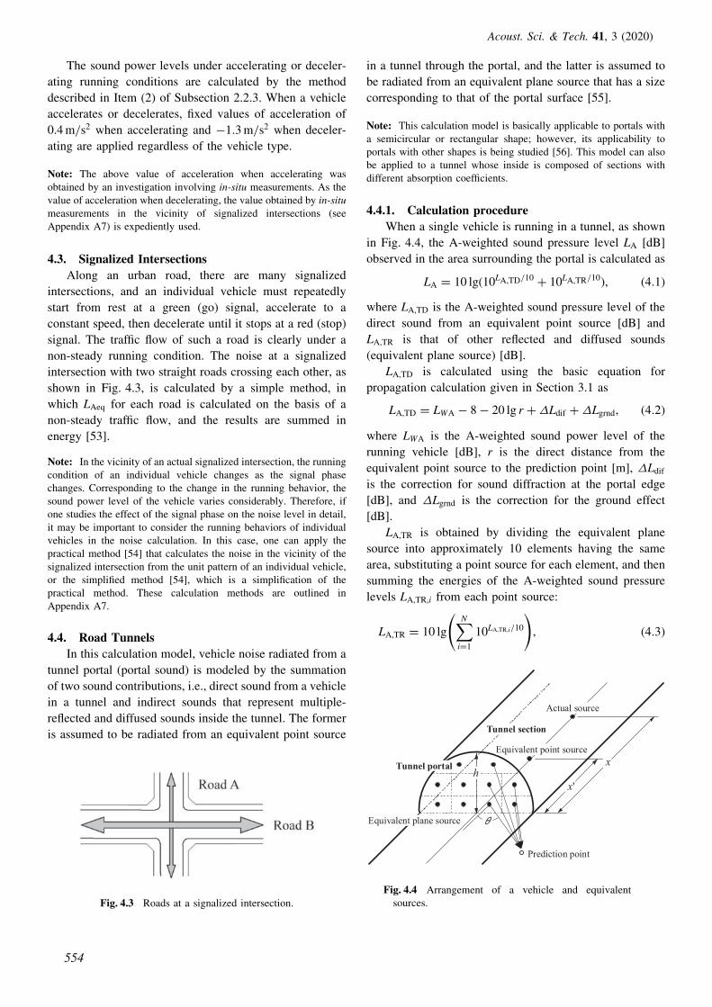
The sound power levels under accelerating or deceler-

ating running conditions are calculated by the method

described in Item (2) of Subsection 2.2.3. When a vehicle

accelerates or decelerates, fixed values of acceleration of

0.4 m/s2 when accelerating and �1:3 m/s2 when deceler-

ating are applied regardless of the vehicle type.

Note: The above value of acceleration when accelerating wasobtained by an investigation involving in-situ measurements. As thevalue of acceleration when decelerating, the value obtained by in-situmeasurements in the vicinity of signalized intersections (seeAppendix A7) is expediently used.

4.3. Signalized Intersections

Along an urban road, there are many signalized

intersections, and an individual vehicle must repeatedly

start from rest at a green (go) signal, accelerate to a

constant speed, then decelerate until it stops at a red (stop)

signal. The traffic flow of such a road is clearly under a

non-steady running condition. The noise at a signalized

intersection with two straight roads crossing each other, as

shown in Fig. 4.3, is calculated by a simple method, in

which LAeq for each road is calculated on the basis of a

non-steady traffic flow, and the results are summed in

energy [53].

Note: In the vicinity of an actual signalized intersection, the runningcondition of an individual vehicle changes as the signal phasechanges. Corresponding to the change in the running behavior, thesound power level of the vehicle varies considerably. Therefore, ifone studies the effect of the signal phase on the noise level in detail,it may be important to consider the running behaviors of individualvehicles in the noise calculation. In this case, one can apply thepractical method [54] that calculates the noise in the vicinity of thesignalized intersection from the unit pattern of an individual vehicle,or the simplified method [54], which is a simplification of thepractical method. These calculation methods are outlined inAppendix A7.

4.4. Road Tunnels

In this calculation model, vehicle noise radiated from a

tunnel portal (portal sound) is modeled by the summation

of two sound contributions, i.e., direct sound from a vehicle

in a tunnel and indirect sounds that represent multiple-

reflected and diffused sounds inside the tunnel. The former

is assumed to be radiated from an equivalent point source

in a tunnel through the portal, and the latter is assumed to

be radiated from an equivalent plane source that has a size

corresponding to that of the portal surface [55].

Note: This calculation model is basically applicable to portals witha semicircular or rectangular shape; however, its applicability toportals with other shapes is being studied [56]. This model can alsobe applied to a tunnel whose inside is composed of sections withdifferent absorption coefficients.

4.4.1. Calculation procedure

When a single vehicle is running in a tunnel, as shown

in Fig. 4.4, the A-weighted sound pressure level LA [dB]

observed in the area surrounding the portal is calculated as

LA ¼ 10 lgð10LA,TD=10 þ 10LA,TR=10Þ; ð4:1Þ

where LA,TD is the A-weighted sound pressure level of the

direct sound from an equivalent point source [dB] and

LA,TR is that of other reflected and diffused sounds

(equivalent plane source) [dB].

LA,TD is calculated using the basic equation for

propagation calculation given in Section 3.1 as

LA,TD ¼ LWA � 8� 20 lg r þ�Ldif þ�Lgrnd; ð4:2Þ

where LWA is the A-weighted sound power level of the

running vehicle [dB], r is the direct distance from the

equivalent point source to the prediction point [m], �Ldif

is the correction for sound diffraction at the portal edge

[dB], and �Lgrnd is the correction for the ground effect

[dB].

LA,TR is obtained by dividing the equivalent plane

source into approximately 10 elements having the same

area, substituting a point source for each element, and then

summing the energies of the A-weighted sound pressure

levels LA,TR;i from each point source:

LA,TR ¼ 10 lgXNi¼1

10LA,TR;i=10

!; ð4:3Þ

Fig. 4.3 Roads at a signalized intersection.

Equivalent point source

Actual source

Tunnel portal

Tunnel section

Equivalent plane source

x'

x

Prediction point

h

Fig. 4.4 Arrangement of a vehicle and equivalentsources.

Acoust. Sci. & Tech. 41, 3 (2020)

554

LA,TR;i ¼ L0WA,R � 8� 20 lg ri þ�Ldif;i þ�Lgrnd;i

þ n � 10 lgðcos �iÞ; ð4:4Þ

n ¼ nað1� e�nbxÞ; ð4:5Þ

L0WA,R ¼ LWA,R � 10 lgN; ð4:6Þ

where ri is the direct distance from the ith equivalent plane

source to the prediction point [m], �i is the angle between

the vector connecting the prediction point from the ith

equivalent plane source and the running direction of

vehicles on the road, and n is the directivity coefficient

for the whole equivalent plane source, calculated using

Eq. (4.5) with the real distance x [m] along the lane from

the tunnel portal to the real point source [57]. The values

in Table 4.3 are used for na and nb. N is the number of

elements into which the plane source is divided, LWA,R is

the A-weighted sound power level of the plane source [dB],

and L0WA,R is the A-weighted sound power level when the

divided elements of the plane source are considered as

point sources [dB].

4.4.2. Location and sound power level of equivalent

point source

The sound power level of the equivalent point source is

specified as that of the actual sound source (running

vehicle), and its position x0 (distance from the portal) [m] is

calculated by applying the parameter related to absorption

in the tunnel, a, and the actual distance from the portal to

the vehicle x [m] as

x0 ¼ ax: ð4:7Þ

If the tunnel is composed of several sections with different

absorption coefficients, a is calculated as

a ¼

Xi¼1

ðaixiÞXi¼1

xi; ð4:8Þ

where ai is the parameter related to absorption in the ith

section and xi is the length of the ith section [m].

The sound power level of the equivalent plane source

LWA,R [dB] set at the portal plane position is calculated by

subtracting the A-weighted sound power PA,D [W] of the

sound radiated as direct sound from the A-weighted sound

power PA,T [W] of all sound radiated from the portal. It is

calculated as

LWA,R ¼ 10 lgPA,T � PA,D

10�12

� �: ð4:9Þ

If the tunnel has a semicircular portal with radius h [m],

PA,T and PA,D are calculated as

PA,T ¼PA

21�

axffiffiffiffiffiffiffiffiffiffiffiffiffiffiffiffiffiffiffiffih2 þ ðaxÞ2

p( )

; ð4:10Þ

PA,D ¼PA

21�

xffiffiffiffiffiffiffiffiffiffiffiffiffiffiffih2 þ x2p

� �; ð4:11Þ

where PA is the A-weighted sound power of the actual

source [W].

If the tunnel has a rectangular portal with width 2w [m]

and height h [m], PA,T and PA,D are calculated as

PA,T ¼PA

�tan�1 whffiffiffiffiffiffiffiffiffiffiffiffiffiffiffiffiffiffiffiffiffiffiffiffiffiffiffiffiffiffiffiffiffiffiffiffiffiffiffiffiffiffiffiffiffiffiffiffi

ðaxÞ4 þ ðw2 þ h2Þ � ðaxÞ2p

( ); ð4:12Þ

PA,D ¼PA

�tan�1 whffiffiffiffiffiffiffiffiffiffiffiffiffiffiffiffiffiffiffiffiffiffiffiffiffiffiffiffiffiffiffiffiffiffiffiffiffi

x4 þ ðw2 þ h2Þ � x2p

( ): ð4:13Þ

4.4.3. Parameter related to absorption inside a tunnel

For the parameter related to sound absorption inside

a tunnel a, the values shown in Table 4.4 are applied

depending on the type of pavement on the road surface.

Note: The relationship between a and the mean absorptioncoefficient of the inner wall of a tunnel A,RTN (refer to Subsec-tion 3.5.3) has been investigated, and the value of a can be estimatedby applying the mean absorption coefficient A,RTN [55,56].

4.5. Depressed and Semi-Underground Roads

A depressed road is defined as a road whose surface

is lower than the surrounding ground and has artificial

sidewall structures (retained walls). If a depressed road

has a horizontal overhang structure on the ceiling, it is

referred to as a semi-underground road in this model. On a

depressed road, multiple sound reflections may occur

between sidewalls. In contrast, on a semi-underground

road, multiple sound reflections tend to occur in the space

surrounded by the road surface, the sidewalls, and the

ceiling. To calculate sound propagation from a depressed/

semi-underground road with these characteristics, several

methods can be used. Among these methods, a calculation

method using a slit method (image source method) and a

Table 4.3 Parameters related to the directivity ofequivalent plane source.

Wall surface condition na nb

Without absorption measure 1.6 0.1

Absorption measure on sidewalls — —

Absorption measure on entire wall — —

Table 4.4 Parameter a related to absorption in tunnel.

Wall surface conditionDense asphalt

pavementDrainage asphalt

pavement

Without absorption measure 0.04 0.1

Absorption measure on sidewalls — 0.4

Absorption measure on entire wall 0.6 —


555

simple method assuming a directional point source model

are provided here. If a more precise prediction is required,

wave-based numerical analysis (see Appendix A6) or a

scale-model experiment [22] is available.

Note: Correction for the noise mitigation effect of absorptivelouvers [58], which are installed on the aperture of a semi-underground road, is applicable only for the simple calculationmethod using a directional point source model.

4.5.1. Slit method (image source method)

(1) Scope

The slit method is applied to depressed roads and semi-

underground roads where the width of the aperture above

the road is at least approximately 75% of the road width.

(2) Basic equations

As shown in Fig. 4.5, the actual source is denoted as

S0, and mirror-image sources, which are the origins of

sound sources reflected by the sidewalls, are denoted as

S1 to Sn. The A-weighted sound pressure level LA [dB] at

prediction point P is calculated as

LA ¼ 10 lg 10LA,0=10 þXNi¼1

fð1� A,RTNÞi � 10LA;i=10g

" #;

ð4:14Þwhere LA,0 is the contribution to the A-weighted sound

pressure level of the actual source [dB], which is calculated

using Eq. (3.1), LA;i is the contribution to the A-weighted

sound pressure level of the ith mirror-image source [dB],

n is the number of mirror-image sources (number of

reflections), and A,RTN is the absorption coefficient of the

sidewall surface (see Subsection 3.5.3).

The contribution from a mirror-image source LA;i is

calculated as

LA;i ¼ LWA � 8� 20 lg ri þ�Lcor;i þ�Lrefl,slit;i; ð4:15Þ

where LWA is the A-weighted sound power level of a

running vehicle [dB], ri is the distance from the ith mirror-

image source to the prediction point [m], �Lcor;i is the

correction for sound attenuation during the propagation

from the ith mirror-image source to the prediction point

[dB], and �Lrefl,slit;i is the correction for the reflection at a

slit part against the ith mirror image source [dB] (refer to

Section 3.5).

Note: In the calculation of the slit method, since the convergencewill be slow even if the number of reflections is increased, one canend at an appropriate number of reflections, but at least tworeflections must be used.

4.5.2. Simple calculation method using a directional

point source model

(1) Scope

This calculation method is applied to the case where

both left and right sides of the cross section of a semi-

underground road are symmetric, and the traffic flows

(composition of vehicle classification and traffic volume)

on the lanes with traffic moving in opposite directions are

almost equivalent.

(2) Basic equations

The A-weighted sound pressure level LA observed at

prediction point P is calculated by considering propagation

in a hemi-free field and an equivalent directional point

source located at the center of an aperture (see Fig. 4.6) as

LA ¼ LWA,su þ 10 lgfaþ ð1� aÞ cosnð�Þ ’g� 8� 20 lg r; ð4:16Þ

nð�Þ ¼ nmax sin� �; ð4:17Þwhere a, nmax, and � are parameters for the directivity of

each equivalent point source and r is the distance from the

equivalent point source S0 to prediction point P [m]. LWA,su

is the apparent sound power level of the equivalent

directional point source S0 determined from the direction

of ’ ¼ 0 [deg] in the coordinate system shown in Fig. 4.6,

given by

LWA,su ¼ LWA þ�Ldim,su þ�Ldir,su

þ�Labs,su þ�Llouver;ð4:18Þ

where LWA is the A-weighted sound power level of a

running vehicle [dB], �Ldim,su is the correction for the

dimensions of a semi-underground road structure [dB],

�Ldir,su is the correction for the directivity of an equivalent

source, �Labs,su is the correction for the absorption in a

θ

φ

Prediction pointP

S r

S’

Width of road L

Height H

Width of apertureW

Absorption coefficient αA,RTN

Fig. 4.6 Coordinate system for calculation of semi-underground roads.

Fig. 4.5 Actual source and mirror-image source groupsof a depressed road.

Acoust. Sci. & Tech. 41, 3 (2020)

556

semi-underground road [dB], and �Llouver is the correction

for the noise mitigation effect of absorptive louvers when

the louvers are installed on the aperture of a semi-

underground road [dB].

�Ldim,su is calculated using the absorption coefficient of

the road surface A,RTN considering the spectrum of typical

road traffic noise, the width of the road L [m], the width

of the aperture W [m], and the height H [m] (see Fig. 4.6)

as [59]

�Ldim,su ¼ 10 lg

�2

�tan�1 W

2Hþ�WH

3L2

þðL�WÞð1� A,RTNÞW

fLA,RTN þ ð1� A,RTNÞWgL

�:

ð4:19Þ

The values given in Table 4.5 for a, nmax, �, and �Ldir,su

for each dimension are applied, which are derived from the

results of scale-model experiments and numerical analysis

based on wave theory [60,61]. The value for A,RTN is 0

for a dense asphalt pavement. In the case of a porous

asphalt pavement, values determined on the basis of in-situ

measurement results are used as A,RTN [62]. The value for

�Labs,su is 0 dB when the wall surface of the inner structure

has a reflective finish and �1 dB when it has an absorptive

finish. An example of a directivity pattern calculated using

the values in Table 4.5 is shown in Fig. 4.7. The value for

�Llouver is 0 dB when no absorptive louvers are installed.

When louvers are installed, the value determined based on

the results of in-situ measurement and scale model experi-

ment is used [63].

(3) Correction for diffraction by noise barriers

If a noise barrier is installed in the vicinity of an

aperture of a semi-underground road, the A-weighted

sound pressure level LA [dB] at prediction point P is

calculated as

Table 4.5 Parameters for directivity of equivalent point source.

Inner structure of Inner structure of

Road Over- Aperture widthsemi-underground road has a semi-underground road has an

width hang (as percentage)reflective finish absorptive finish

lengtha nmax �

�Ldir,su a nmax ��Ldir,su

[dB] [dB]

5 m (25%) 0.15 1.4 1.7 1.61 0.05 2.0 1.2 2.68

1 m 7.5 m (37.5%) 0.15 1.2 1.7 1.45 0.05 2.0 1.2 2.68

20 m10 m (50%) 0.15 1.0 2.0 1.20 0.05 2.1 1.2 2.77

5 m (25%)0.13 1.5 2.0 1.62 0.03 1.9 1.1 2.77

4 m7.5 m (37.5%)

10 m (50%) 0.13 1.2 2.0 1.40 0.03 2.1 0.9 3.15

5 m to 7.5 m0.15 1.6 2.2 1.58 — — — —

1 m(16.7% to 25%)

10 m (33%) 0.15 1.2 2.0 1.36 — — — —

30 m15 m (50%) 0.15 1.0 2.0 1.20 — — — —

5 m to 7.5 m0.12 1.6 2.2 1.65 — — — —

4 m(16.7% to 25%)

10 m (33%) 0.12 1.2 2.0 1.42 0.03 1.9 1.0 2.99

15 m (50%) 0.12 1.0 2.0 1.25 0.03 2.0 1.0 3.09

Fig. 4.7 Example of radiation directivity of noise (road width: 20 m, overhang width: 4 m, aperture width: 7.5 m, reflectivefinish inside).


557

LA ¼ L0A þ�Ldif,sb; ð4:20Þ

where L0A is the A-weighted sound pressure level calcu-

lated at hypothetical prediction point P0 [dB]; P0 is located

in the direction from S0 to the top edge of a noise barrier O

(diffraction point) and S0P ¼ S0P0 (see Fig. 4.8). �Ldif,sb is

the correction for diffraction calculated with the path

difference � [m], determined from the path from S0 to P

through O [dB].

Note: If a semi-underground road with an identical cross sectionis straight for a sufficient length, discrete equivalent point sources inline can be treated as a line source. From this concept, a method forproviding directivity as a function of only ’ is being studied [64].

4.6. Flat Roads with an Overhead Viaduct, Double-

Deck Viaducts

4.6.1. Types of underside of viaduct and calculation

methods

The underside of a viaduct may have a smooth and flat

shape, or an uneven shape, as shown in Fig. 4.9. Depend-

ing on the shape of the underside, either the slit method or

the scattered reflection method is applied, as described

next. For ordinal noise calculation, the former method is

generally applied, while the latter is applied if the

unevenness is not negligible [46,65]. These methods are

applicable to the cases in which a noise barrier is not

installed on a flat road with an overhead viaduct, or a noise

barrier is installed only on a single side of a flat road. The

concept of the calculation for double-deck viaducts is the

same as that for flat roads with overhead viaducts. When

especially high barriers are installed on both sides of a flat

road with an overhead viaduct, neither the slit method nor

the scattered reflection method can be applied because the

sound field is complicated in the space surrounded by the

road surface, the noise barriers, and the underside of the

viaduct. In this case, wave-based numerical analysis is

applied (see Appendix A6).

Note 1: In addition to the void slab structure shown in Fig. 4.9,structures with flat sound-absorbing boards installed on the undersidecan be regarded as ‘‘flat type.’’

Note 2: When the overhead viaduct is wide, for example, owing to atollgate, the effect of high-order reflected sound cannot be ignored.The boundary energy integral equation method has been proposed asan energy-based noise prediction method for such cases [66].

Note 3: The geometrical ray-tracing method is one of the qualitativeprediction methods and effective for investigating the range of thereflected sound from the underside of a viaduct.

4.6.2. Slit method (image source method)

As shown in Fig. 4.10, consider a case when a noise

barrier is installed on a single side of a flat road. For an

ordinary viaduct road with four to six lanes, consider the

four major sound paths of (a) a direct sound (S to P), (b) a

reflection from the underside of a viaduct road (S0 to P),

and (c) reflections from the underside and ground (S0 to P0

and S00 to P). The A-weighted sound pressure level LA [dB]

at prediction point P is calculated using the following

Fig. 4.9 Shapes of the underside of a viaduct road.

Prediction pointP

P'

O

S'


PO

S'

rr2r1

r1+ r2 - rPrediction point


Fig. 4.8 Geometry for calculation of diffraction effect.

Fig. 4.10 Propagation paths in the slit method.

Acoust. Sci. & Tech. 41, 3 (2020)

558

equation based on the total contribution from these sound

paths:

LA ¼ 10 lgð10LA,0=10 þ 10LA,1=10 þ 10LA,2=10 þ 10LA,3=10Þ;ð4:21Þ

where LA,0, LA,1, LA,2, and LA,3 are the A-weighted sound

pressure levels of the direct sound, the reflection from the

underside of the viaduct, and the reflections from the

underside and ground (S0 to P0 and S00 to P), respectively.

Among them, LA,1, LA,2, and LA,3 are calculated using the

following equation:

LA;i ¼ LWA � 8� 20 lg ri þ�Ldif,sb;i ði ¼ 1 to 3Þ;

þ�Lrefl,slit;i þ�Labs ð4:22Þ

where �Ldif,sb;i is the correction for attenuation due to

the noise barrier for the ith mirror-image source [dB],

�Lrefl,slit;i is the correction for reflection calculated by the

slit method [dB] (see Subsection 3.5.1), and �Labs is the

correction for sound attenuation due to the absorptive

surface [dB]. In some practical cases, it is necessary to

consider a double diffraction at the top of the noise barrier

and the open edge of the slit. For convenience, however,

the edge of the slit is neglected in the calculation of

�Ldif,sb;i, and the noise barrier is neglected in the

calculation of �Lrefl,slit;i. For the case where the underside

of a viaduct is absorptive, the correction for absorption

�Labs is applied (see Subsection 3.5.3).

Since the range of the effect of a reflected sound from

the underside of a viaduct strongly depends on the position

of the sound source, the sound source is set at the center of

an actual lane in the calculation (here, two or more lanes

should not be combined into one hypothetical lane). For

the case when no noise barrier is installed on a flat road,

only the path S0 to P0 is selected to calculate the reflection

from the underside and ground. In the actual calculation,

the term for LA,3 of Eq. (4.21) is ignored, and LA,1 and LA,2

in Eq. (4.22) are calculated by setting �Ldif,sb,1 ¼ 0 and

�Ldif,sb,2 ¼ 0.

Note: Even if the underside of a viaduct is treated with anabsorptive material, the beams of piers may not be absorptive.Therefore, it is desirable to use a mean sound absorption coefficientweighted by the ratio of the areas of the absorptive and non-absorptive surfaces.

4.6.3. Scattered reflection method [47]

(1) Equations

As shown in Fig. 4.11, a scattered reflection surface B

with a width of the viaduct is assumed beneath girders on

the underside of the viaduct above source and prediction

points. Similarly to the slit method, we consider the four

major paths of (a) a direct sound (S to P), (b) the reflection

from the underside of a viaduct (S to P through B), and

(c) the reflections from the underside and ground (S to P0

through B and S to P through B0). The A-weighted sound

pressure level LA [dB] at prediction point P is calculated

using Eq. (4.21). Different from the slit method, however,

the reflected surface B is divided into elements Bj ( j ¼ 1 to

N), and LA,1, LA,2, and LA,3 in Eq. (4.21) are calculated as

LA; j ¼ LWA � 13þ 10 lgXNj¼1

Sj cos �j � cos j � Dj j

r2j R2j

ði ¼ 1 to 3Þ; ð4:23Þ

Dj ¼ 10�Ldif,sb; j=10; ð4:24Þ

where Sj is the area [m2] of element Bj of the scattered

reflection surface B, �j and j are the incidence and

reflection angles at the center of Bj, respectively, rj is the

distance [m] from source point S to the center of Bj, and Rj

is the distance [m] from the center of Bj to prediction

point P (see Fig. 4.12). Dj and �Ldif,sb; j are the diffraction

coefficient and correction [dB] for sound attenuation due to

the noise barrier, respectively, when a point source is set at

the center of Bj, and j (¼ 1� j) and j are the reflection

and absorption coefficients of Bj, respectively. The reflec-

tion angle j is the angle between the normal vector n and

the propagation direction as shown in Fig. 4.12.

If a noise barrier is not installed on the roadside of a flat

road, only the path from S to P0 through B is specified as

the reflection path from the underside and ground. In the

actual calculation, the term for LA,3 of Eq. (4.21) can be

ignored, and LA,2 is calculated using Eq. (4.23) with Dj ¼1. Sources may be combined into a representative hypo-

thetical lane (see Item 1.3.2 (2)).

(2) Calculation settings

When a flat road and an overhead viaduct road are

parallel and the cross sections of the roads are regarded as

being uniform, the scattered reflection surface B is divided

with quadrilateral elements, the width of which is one-

quarter or less of the height H [m] of the surface B. The

ranges of the discrete point sources and of the reflection

surface for the calculation are shown in Table 4.6 and

Fig. 4.13.

P

P'S

Viaduct road

Mirror image ofviaduct road

Scattered reflection surface B

Prediction point

Mirror image of scatteredreflection surface B'

Source

Fig. 4.11 Propagation paths in the scattered reflectionmethod.


559

This method cannot be used if the flat road and the

overhead viaduct road are crossed. When calculating LAeq

in such cases, first, calculate the unit pattern of the reflected

sound from the underside of the viaduct through three-

dimensional calculation (summation of LA,1 to LA,3 in

Eq. (4.21)). Next, for the range from the maximum value

of the unit pattern to approximately �15 dB, add the direct

sound LA,0 using Eq. (4.21); for the other range, omit LA,1

to LA,3, i.e., use only the direct sound LA,0. Lastly, calculate

LAeq from LAE obtained from the total unit pattern.

Note: The direct sound LA,0 is calculated according to Item 1.3.2(3).

5. STRUCTURE-BORNE NOISEOF VIADUCTS

When vehicles run on a viaduct road, noise is generated

by the vibration of the structure, which is referred to as

structure-borne noise of the viaduct. The degree of noise

depends on the type of viaduct and the speed and weight

of vehicles. The noise calculation method is described in

the following [67,68].

5.1. Scope

(1) Type of viaduct

General steel viaducts and concrete viaducts, as shown

in Table 5.1.

(2) Type of vehicle

Only heavy vehicles are considered.

Note: Since the structure-borne noise of viaducts for light vehiclesis relatively minor, it is omitted in this model.

(3) Running speed of vehicles

Applicable for vehicles running at 40 km/h or more.

5.2. Noise Calculation Procedure

5.2.1. Setting of hypothetical sound source

The structure-borne noise of a viaduct is radiated from

(b) When the center of Bj can be seen from P

nRjrj θj

ψj

Bj

Predictionpoint P

Scattered reflectionsurface B

Source S

Viaduct road

Source S

Predictionpoint Pn

θjψj Rj


rj

Bj

(a) When the center of Bj cannot be seen from P

Fig. 4.12 Definition of reflection angle j in thescattered reflection method.

Table 4.6 Calculation conditions for reflection soundfrom the underside of viaduct.

Item Condition

Range of discrete pointsources, xS

xP � ð1:5lB þ 70Þ � xS � xP þð1:5lB þ 70Þ

Range of reflectionsurface, xB

xS ��xB � xB � xS þ�xB,�xB ¼ H þ 15

Width (side length) ofquadrilateral element Bi

H=4 or less


0

z

Source S

Predictionpoint P

(0, yP, zP)

(xS, yS, 0)

zB

W

(0, yP, -zP)

Predictionpoint P

(xP , yP, zP)

x

Source S

(a) Cross section

(b) Plan view

Hl B

xB

xS + Δ xB

xP − xB

(xS, yS, 0)


Area of reflective

surface B in the calculation

y

y

Δ

xBΔ

Δ

Fig. 4.13 Calculation conditions in the scattered reflec-tion method.

Acoust. Sci. & Tech. 41, 3 (2020)

560

the entire slab and girder structure. However, for conven-

ience of calculation, an omnidirectional point source is

assumed as an equivalent moving sound source that is

synchronized with the running vehicle. The moving point

source is set on the surface of the underside of the viaduct

(on the bottom edge of the main girders for a girder

structure, or on the bottom surface of a slab for a void slab

structure) at a hypothetical lane that is located directly

beneath the center of each set of lanes traveling in both

directions. In the calculation of LAeq;T , discrete point

sources are set on the hypothetical lane (see Fig. 5.1).

5.2.2. A-weighted sound power level of hypothetical

point source

The A-weighted sound power level of a hypothetical

point source LWA,str [dB] is calculated as

LWA,str ¼ aþ 30 lgV ; ð5:1Þ

where V is the running speed [km/h] and a is the value

allocated to each type of viaduct as given in Table 5.2.

Regarding the type of viaduct, a five-category classification

is recommended. A three-category classification can be

used if the type of viaduct cannot be fixed precisely.

Note 1: The value of a for each type of viaduct was determined bypower-averaging a number of values a, each of which was calculatedusing Eq. (5.1) with measured data for each individual viaduct. Thisprocedure is the same as that for determining the constant valuesused in the equations for sound power level for running vehicles.

Note 2: For other types of viaduct, studies based on in-situinvestigations (Reference R5.2) are necessary [69].

5.2.3. Calculation of unit pattern

The A-weighted sound pressure level of noise propa-

gated from each source point on the hypothetical lane to the

prediction point LA,str [dB] is calculated as

LA,str ¼ LWA,str � 8� 20 lg r þ�Ldif ; ð5:2Þ

where r is the distance from the source point to the

prediction point [m] and �Ldif is the correction to the

structure-borne noise of the viaduct for the sound diffrac-

tion effect due to the shielding by the slab or girder

structure [dB]. �Ldif,sb is used as �Ldif for diffraction

around the I-girders and steel I-girders, and �Ldif,rw is used

for diffraction around the steel box girders, box girders,

and void slab girders, shown in Table 5.1 (see Subsec-

tion 3.2.2).

Note 1: It is not necessary to consider the contribution of the soundreflection from the ground surface in the above calculationprocedure, because its effect is already taken into account whendetermining the constant a in the equation for LWA,str.

Note 2: The correction for the sound diffraction effect due to thestructure-borne noise of the viaduct �Ldif is formulated using a

Table 5.1 Types of viaduct road.

Type Steel viaduct Concrete viaduct

Slab Steel Concrete Concrete

GirderSteel box girder Steel I-girder I-girder

Other than I-girder

structure Box girder Void slab girder

Illustration

Note: The parts colored in black are slabs. All illustrations in this table show concrete slabs.

Fig. 5.1 Arrangement of hypothetical point sources forstructure-borne noise.

Table 5.2 Value of a for each viaduct type.

Type of viaduct a

Steel slab steel box girder 40.7

Steel viaduct Concrete slab steel box girder 35.538.9

Concrete slab steel I-girder 40.4

Concrete I-girder 31.834.8

viaduct Other than I-girder 35.9


561

calculation chart for diffraction [23,24] and the measured spectrumof the structure-borne noise.

The unit pattern of the structure-borne noise is obtained

by applying the above-mentioned calculation to all source

points. The method of calculating LAeq from the unit

pattern is similar to that for calculating vehicle running

noise on general roads.

6. NOISE BEHIND SINGLE BUILDINGAND IN BUILT-UP AREAS

Behind a single building or building complex along the

sides of roads, the road traffic noise is attenuated by their

screening effect. To predict the degree of attenuation,

methods of calculating noise around a single building and

behind a dense building complex are given below using the

following prediction model.

6.1. Noise behind Single Building

As a method of calculating noise around a single

building along the sides of roads, the following prediction

model is considered. In this method, only the diffraction by

the top of a single building is considered (referred to as the

one-path method), and diffraction by the sides of the

building is ignored.

Buildings are thick obstacles with limited lengths.

Around a single building, it is necessary to consider the

noise attenuation due to the screening effect of the

building. Thus, LAeq behind a single building is calculated

by applying the methods of calculating the correction for

diffraction caused by a finite-length barrier (Subsection

3.2.2(3)) and diffracted sounds (Subsection 3.2.4), and

finally summing the direct sounds and diffracted sounds

(see Fig. 6.1(a)). In this model, the building is represented

by a rectangular parallelepiped, and it is assumed that there

is no sound absorption on the walls of the building.

The unit pattern is calculated as

LA0;i ¼ LWA;i � 8� 20 lg r0;i þ�Lbldg;i; ð6:1Þ

where LA0;i is the A-weighted sound pressure level [dB] of

the direct sound component (or diffracted sound compo-

nent) from Si. �Lbldg;i is the correction for the diffraction

by the building [dB]. r0;i is the distance [m] between the

sound source Si and the receiver P.

In the calculation of the unit pattern, as shown in

Fig. 6.1(b), when line segment SP crosses the building, the

building is treated as an infinite-length barrier with depth

D [m], and then �Lbldg is calculated similarly to �Ldif,tb

using Eq. (3.9). When the line segment does not cross the

building, it is concluded that there is no building and then

�Lbldg is equal to zero.

Note 1: LA0;i calculated by the one-path method mentioned abovewidely changes when the line segment SP is positioned near the end

of the building. Therefore, the method cannot be applied in the caseof calculating a precise unit pattern. The detailed calculation methodconsidering the diffraction by the top and sides of the building isprovided in the literature [70,71].

Note 2: The calculated LAeq using the one-path method and thatusing the method considering the diffraction by the top and sides ofthe building are approximately equal except only in very specialcases [71].

6.2. Noise behind Building Complex

In this prediction model, a practical calculation method

is provided for predicting noise behind a dense building

complex. It is assumed for the methods described here that

the detached houses are of standard size in Japan; therefore,

the calculation methods are not applicable to built-up areas

with buildings of different sizes and different conditions of

building locations.

It is recommended to employ the advanced calculation

method, which is described in Appendix A8, in certain

situations, for example, when the unit patterns must be

calculated more correctly for planning countermeasures

against noise or when the detailed diffraction and reflection

by the sides of the buildings must be considered.

6.2.1. Practical calculation method using a point

source model [72]

When detached houses are located in an area facing a

plane road, noise behind the detached houses attenuates

owing to the screening effect of the houses. In this case, the

(a) Direct sound (diffracted sound)

(b) Calculation of ΔLbldg by one-path method

Fig. 6.1 Calculation of noise behind a single building.

Acoust. Sci. & Tech. 41, 3 (2020)

562

A-weighted sound pressure level LA;i at a prediction point

from the ith source position is calculated as

LA;i ¼ LWA;i � 8� 20 lg ri þ�LB;i; ð6:2Þ

where LWA;i is the A-weighted sound power level of a

single running vehicle at the ith source position [dB] and riis the direct distance from the ith source position to the

prediction point [m]. �LB;i denotes the correction related

to the attenuation due to the detached houses along the

propagation path from the ith source position to the

prediction point [dB]. It is given by the following equation.

The suffix i for the source position is hereafter omitted for

simplicity of notation.

�LB ¼ p ��LBB þ q

p ¼ 0:017ðH � hp � 8:8Þ þ 1

q ¼ �0:063ðH � hp � 8:8Þð6:3Þ

Here, H is the height of the detached houses [m] and hp is

the height of the prediction point [m]. �LBB is the

correction value [dB] when H is 10 m and hp is 1.2 m

and is given by

�LBB ¼ 10 lg b0 þ b1 ��

�þ b2 � 10�0:0904��dSP

� �; ð6:4Þ

where b0 ¼ 0:046, b1 ¼ 1:01, and b2 ¼ 0:554. In Eq. (6.4),

the term related to �=� indicates the direct sound from the

source to the prediction point. � and � are the perspective

angles [rad] from the prediction point to a part of the target

road of 10 m length where the sound source S is the

midpoint, as shown in Figs. 6.2 and 6.3, in the cases with

and without detached houses, respectively.

The term related to 10�0:0904��dSP indicates sounds other

than the direct sounds. As shown in Fig. 6.4, dSP is the

horizontal distance between S and P. A 15-m-wide

rectangular area is assumed between S and P, and the

density of the houses � (the ratio of the location area of the

detached houses to the rectangular area) is calculated.

Equations (6.3) and (6.4) were deduced from the results

of scale-model experiments assuming residential areas in

which many detached houses of standard size in Japan

were located. In the experiments, the horizontal distances

between the prediction points and the target roads were 20

to 50 m. The ratio of the total area of the detached houses to

the location area was in the range from 0.16 to 0.34. The

heights (H) of the detached houses were 4 to 10 m and the

heights (hp) of the receiver were 1.2 to 9.2 m. Therefore,

this calculation method is valid in these ranges. Further-

more, hp should be less than H. If the heights of the

detached houses are different from each other and the roofs

are not flat, the mean height of the detached houses can be

used as H [73].

6.2.2. Simplifying the computation of practical calcu-

lation method [74,75]

Equation (6.4) is expressed as a sum of the constant b0,

the component of direct sound, and the component other

than the direct sound (referred to as Eoth). In the case of the

buildings lying evenly in the target area, the error of �LBB

would be maintained under 0.5 dB if Eoth was omitted by

the following three judgement procedures.Fig. 6.2 Perspective angles to the road � in the cases

without detached houses.

Fig. 6.3 Perspective angles to the road � in the caseswith detached houses.

Fig. 6.4 Horizontal distance between S and P, dSP, andbuilding density � in the area of 15 m width and dSP

length.


563

(1) Judgement procedure using horizontal distance

between the source and prediction point

When the distance from the source to the prediction

point (dSP) exceeds 254 m, Eoth can be set to zero and the

density of the houses (�) need not to be calculated.

This is an easy procedure because the judgement can be

implemented only using dSP.

(2) Judgement procedure considering the direct sound

When dSP is less than 254 m, the shortest omittable

distance (d�SP) from the prediction point P to the source S is

calculated as

d�SP ¼ �234�

�

� �3

þ 659�

�

� �2

� 386�

�

� �þ 220; ð6:5Þ

and when dSP exceeds d�SP, Eoth can be set to zero.

Even though the calculation using Eq. (6.5) is required,

this judgement is useful since it can be implemented

regardless of the visibility of the source from the prediction

point.

(3) Judgement procedure when the source is invisible

from the prediction point

When houses are uniformly distributed and � is zero,

point sound sources are selected in order of increasing

distance from the prediction point and used to calculate

� � dSP. Once � � dSP exceeds 22.1, Eoth can be set to zero for

the sound source point and subsequent points.

This procedure enables Eoth to be set to zero and the

calculation of � for all sources of � ¼ 0 to be omitted

before the distance becomes d�SP. Although this is a more

complicated procedure than (1) and (2), it can be useful

when the calculation cost should be minimized.

Note: Only the contribution of sounds propagating into the buildingcomplex is considered in this prediction model. When the height ofthe receiver is greater than those of the buildings or noise is predictedfor a viaduct with a noise barrier or for a banked road, it is necessaryto consider the contribution of sounds propagating over the buildings.

APPENDICES

Appendix A1 SOUND POWER SPECTRAOF VEHICLE NOISE

In this appendix, the frequency characteristics (power

spectrum) of running vehicle noise on dense asphalt,

porous asphalt, and KOUKINOU II pavements are describ-

ed.

A1.1. Power Spectrum for Dense Asphalt Pavement

The A-weighted sound power level for each frequency

band (1=n-octave band) on a dense asphalt pavement is

given by the following method. For the frequency bands,

the center frequencies for the octave bands are from 63 Hz

to 4 kHz, and those for the 1/3-octave bands are from

50 Hz to 5 kHz. The A-weighted band power level LWAð fc;iÞ[dB] for the ith center frequency fc;i [Hz] is calculated as

LWAð fc;iÞ ¼ LWA þ�LWAð fc;iÞ; ðA1.1Þ

where LWA is the A-weighted sound power level of the

road vehicle on a dense asphalt pavement [dB] (see

Subsection 2.2.2) and �LWAð fc;iÞ is the A-weighted rela-

tive power level for the frequency band of fc;i [dB].

Table A1.1 and Fig. A1.1 show the representative A-

weighted relative power level �LWAð fc;iÞ on a dense

asphalt pavement.

A1.2. Power Spectrum for Porous Asphalt Pavement

The A-weighted band power level LWAð fc;iÞ for the

center frequency fc;i [Hz] on a porous asphalt pavement

is given by Eq. (A1.1). In the equation, LWA is the A-

weighted sound power level on porous asphalt (see

Subsection 2.2.3), which was determined using the meas-

urement data for the steady running condition on express-

ways where the elapsed time since the construction of the

pavement was within 11 years, and �LWAð fc;iÞ is the

representative A-weighted relative power level shown in

Table A1.2 and Fig. A1.1.

Table A1.1 A-weighted relative band power level�LWAð fc;iÞ on dense asphalt pavement.

Center frequency A-weighted relative band power level [dB]

[Hz] Octave band 1/3-octave band

50 �38:763 63 �30:2 �35:4

80 �32:7

100 �29:8125 125 �22:1 �27:2

160 �25:0

200 �21:2250 250 �14:0 �18:8

315 �17:2

400 �15:4500 500 �7:9 �13:3

630 �10:6

800 �8:31,000 1,000 �3:0 �7:2

1,250 �8:0

1,600 �9:32,000 2,000 �6:0 �10:8

2,500 �13:2

3,150 �15:84,000 4,000 �13:4 �18:8

5,000 �21:7

Overall 0.0 0.0

Acoust. Sci. & Tech. 41, 3 (2020)

564

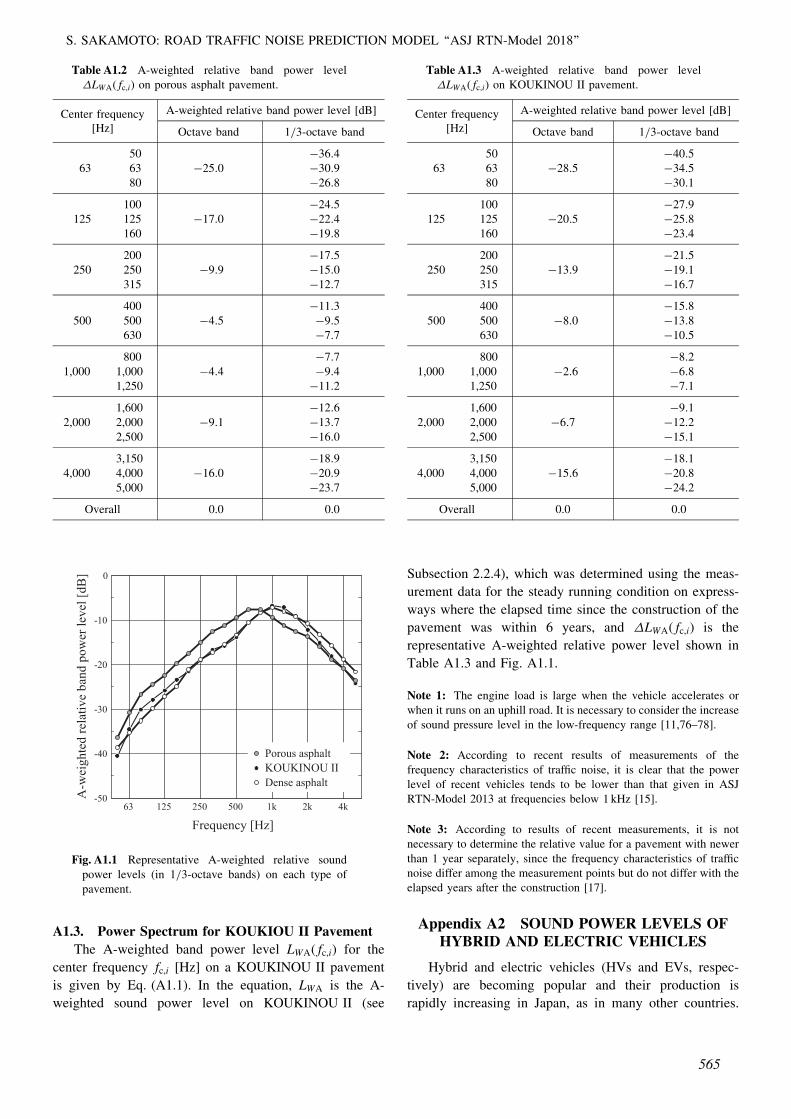
A1.3. Power Spectrum for KOUKIOU II Pavement

The A-weighted band power level LWAð fc;iÞ for the

center frequency fc;i [Hz] on a KOUKINOU II pavement

is given by Eq. (A1.1). In the equation, LWA is the A-

weighted sound power level on KOUKINOU II (see

Subsection 2.2.4), which was determined using the meas-

urement data for the steady running condition on express-

ways where the elapsed time since the construction of the

pavement was within 6 years, and �LWAð fc;iÞ is the

representative A-weighted relative power level shown in

Table A1.3 and Fig. A1.1.

Note 1: The engine load is large when the vehicle accelerates orwhen it runs on an uphill road. It is necessary to consider the increaseof sound pressure level in the low-frequency range [11,76–78].

Note 2: According to recent results of measurements of thefrequency characteristics of traffic noise, it is clear that the powerlevel of recent vehicles tends to be lower than that given in ASJRTN-Model 2013 at frequencies below 1 kHz [15].

Note 3: According to results of recent measurements, it is notnecessary to determine the relative value for a pavement with newerthan 1 year separately, since the frequency characteristics of trafficnoise differ among the measurement points but do not differ with theelapsed years after the construction [17].

Appendix A2 SOUND POWER LEVELS OFHYBRID AND ELECTRIC VEHICLES

Hybrid and electric vehicles (HVs and EVs, respec-

tively) are becoming popular and their production is

rapidly increasing in Japan, as in many other countries.

63 125 250 500 1k 2k 4k -50

-40

-30

-20

-10

0

Frequency [Hz]

A-w

eigh

ted

rela

tive

band

pow

er le

vel [

dB]

Porous asphalt

Dense asphaltKOUKINOU II

Fig. A1.1 Representative A-weighted relative soundpower levels (in 1/3-octave bands) on each type ofpavement.

Table A1.2 A-weighted relative band power level�LWAð fc;iÞ on porous asphalt pavement.



50 �36:463 63 �25:0 �30:9

80 �26:8

100 �24:5125 125 �17:0 �22:4

160 �19:8

200 �17:5250 250 �9:9 �15:0

315 �12:7

400 �11:3500 500 �4:5 �9:5

630 �7:7

800 �7:71,000 1,000 �4:4 �9:4

1,250 �11:2

1,600 �12:62,000 2,000 �9:1 �13:7

2,500 �16:0

3,150 �18:94,000 4,000 �16:0 �20:9

5,000 �23:7

Overall 0.0 0.0

Table A1.3 A-weighted relative band power level�LWAð fc;iÞ on KOUKINOU II pavement.



50 �40:563 63 �28:5 �34:5

80 �30:1

100 �27:9125 125 �20:5 �25:8

160 �23:4

200 �21:5250 250 �13:9 �19:1

315 �16:7

400 �15:8500 500 �8:0 �13:8

630 �10:5

800 �8:21,000 1,000 �2:6 �6:8

1,250 �7:1

1,600 �9:12,000 2,000 �6:7 �12:2

2,500 �15:1

3,150 �18:14,000 4,000 �15:6 �20:8

5,000 �24:2

Overall 0.0 0.0


565

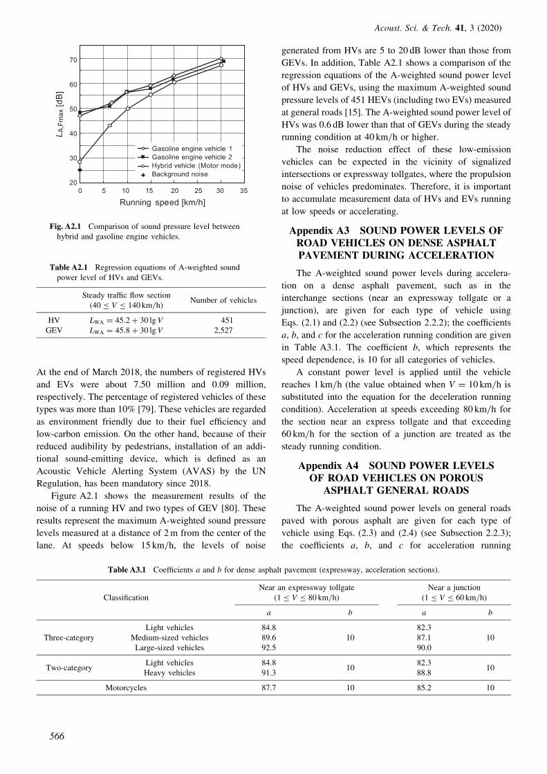
At the end of March 2018, the numbers of registered HVs

and EVs were about 7.50 million and 0.09 million,

respectively. The percentage of registered vehicles of these

types was more than 10% [79]. These vehicles are regarded

as environment friendly due to their fuel efficiency and

low-carbon emission. On the other hand, because of their

reduced audibility by pedestrians, installation of an addi-

tional sound-emitting device, which is defined as an

Acoustic Vehicle Alerting System (AVAS) by the UN

Regulation, has been mandatory since 2018.

Figure A2.1 shows the measurement results of the

noise of a running HV and two types of GEV [80]. These

results represent the maximum A-weighted sound pressure

levels measured at a distance of 2 m from the center of the

lane. At speeds below 15 km/h, the levels of noise

generated from HVs are 5 to 20 dB lower than those from

GEVs. In addition, Table A2.1 shows a comparison of the

regression equations of the A-weighted sound power level

of HVs and GEVs, using the maximum A-weighted sound

pressure levels of 451 HEVs (including two EVs) measured

at general roads [15]. The A-weighted sound power level of

HVs was 0.6 dB lower than that of GEVs during the steady

running condition at 40 km/h or higher.

The noise reduction effect of these low-emission

vehicles can be expected in the vicinity of signalized

intersections or expressway tollgates, where the propulsion

noise of vehicles predominates. Therefore, it is important

to accumulate measurement data of HVs and EVs running

at low speeds or accelerating.

Appendix A3 SOUND POWER LEVELS OFROAD VEHICLES ON DENSE ASPHALTPAVEMENT DURING ACCELERATION

The A-weighted sound power levels during accelera-

tion on a dense asphalt pavement, such as in the

interchange sections (near an expressway tollgate or a

junction), are given for each type of vehicle using

Eqs. (2.1) and (2.2) (see Subsection 2.2.2); the coefficients

a, b, and c for the acceleration running condition are given

in Table A3.1. The coefficient b, which represents the

speed dependence, is 10 for all categories of vehicles.

A constant power level is applied until the vehicle

reaches 1 km/h (the value obtained when V ¼ 10 km/h is

substituted into the equation for the deceleration running

condition). Acceleration at speeds exceeding 80 km/h for

the section near an express tollgate and that exceeding

60 km/h for the section of a junction are treated as the

steady running condition.

Appendix A4 SOUND POWER LEVELSOF ROAD VEHICLES ON POROUS

ASPHALT GENERAL ROADS

The A-weighted sound power levels on general roads

paved with porous asphalt are given for each type of

vehicle using Eqs. (2.3) and (2.4) (see Subsection 2.2.3);

the coefficients a, b, and c for acceleration running

0 5 10 15 20 25 30 35


70

60

50

40

30

20

Gasoline engine vehicle 1Gasoline engine vehicle 2Hybrid vehicle (Motor mode)Background noise

L A,F

max

[dB

]

Fig. A2.1 Comparison of sound pressure level betweenhybrid and gasoline engine vehicles.

Table A2.1 Regression equations of A-weighted soundpower level of HVs and GEVs.

Steady traffic flow section(40 � V � 140 km/h)

Number of vehicles

HV LWA ¼ 45:2þ 30 lgV 451GEV LWA ¼ 45:8þ 30 lgV 2,527

Table A3.1 Coefficients a and b for dense asphalt pavement (expressway, acceleration sections).

Near an expressway tollgate Near a junctionClassification (1 � V � 80 km/h) (1 � V � 60 km/h)

a b a b

Light vehicles 84.8 82.3Three-category Medium-sized vehicles 89.6 10 87.1 10

Large-sized vehicles 92.5 90.0


1082.3

10Heavy vehicles 91.3 88.8

Motorcycles 87.7 10 85.2 10

Acoust. Sci. & Tech. 41, 3 (2020)

566

condition are given in Table A4.1. The vehicle speed V is

in the range from 40 to 80 km/h for the steady traffic flow

section and from 10 to 60 km/h for the non-steady traffic

flow section. The coefficient b, which represents the speed

dependence, is 30 and 10 for the steady- and non-steady

traffic flow sections, respectively. The coefficient c is

always 0 for motorcycles.

Appendix A5 CALCULATION OFFREQUENCY-DEPENDENT

PROPAGATIOIN

In this appendix, a general energy-based calculation

method for frequency-dependent sound propagation, which

is not limited to road traffic noise, is presented.

A5.1. Basic Equations for Propagation

Consider point source S and prediction point P on a flat

ground surface as shown in Fig. A5.1. Generally, the

propagation paths to be considered are the two paths in

Fig. A5.1(a) when there is no barrier (no diffraction

calculation is required), and the four paths in Fig. A5.1(b)

when there is a barrier. In the prediction of road traffic

noise, however, the numbers of paths to be considered are

one and two without and with a barrier, respectively,

because the sound source is placed on a road surface. The

A-weighted sound pressure level LA [dB] is calculated

using the following equations. LA in Eq. (A5.1) corre-

sponds to that in Eq. (3.1).

LA ¼ 10 lgXi

10LAð fc;iÞ=10; ðA5.1Þ

LAð fc;iÞ ¼ 10 lgXMm¼1

10LA;mð fc;iÞ=10 þ�Lg,exð fc;iÞ; ðA5.2Þ

LA;mð fc;iÞ ¼ LWAð fc;iÞ � 11� 20 lg rm

þ�Ldif;mð fc;iÞ þ�Lair;mð fc;iÞ:ðA5.3Þ

Here, fc;i is the center frequency [Hz] of the ith band,

LAð fc;iÞ is the A-weighted sound pressure level [dB] for the

frequency band of fc;i, LA;mð fc;iÞ is the A-weighted sound

pressure level [dB] for propagation path m (see Fig. A5.1)

for the frequency band of fc;i, LWAð fc;iÞ is the sound power

level [dB] for the frequency band of fc;i, rm is the

propagation distance [m] for propagation path m (the

direct distance from the sound source or its mirror image

to the prediction point or its mirror image), �Ldif;mð fc;iÞand �Lair;mð fc;iÞ are the correction terms [dB] for prop-

agation path m for diffraction (�Ldif;mð fc;iÞ ¼ 0 dB without

a barrier) and atmospheric absorption, respectively, and

�Lg,exð fc;iÞ is the correction term [dB] for the excess

attenuation due to the ground. The calculation frequencies

fc;i are the 1/3-octave band center frequencies from 100 Hz

to 5 kHz. In the following, the subscript of frequency f and

subscript m representing a propagation path will be omitted

if there is no misunderstanding without them.

Note: In the road traffic noise prediction, firstly, LA is calculatedwith the moving sound source S to obtain the unit pattern; secondly,LEA is obtained from the unit pattern using Eq. (1.11); lastly, LAeq;T

is calculated using Eq. (1.12).

Table A4.1 Coefficients a, b, and c for porous asphalt pavement (general road, steady, and non-steady traffic flowsections).

Steady traffic flow section Non-steady traffic flow sectionClassification (40 � V � 80 km/h) (10 � V � 60 km/h)

a b c a b c

Light vehicles 41.0 7.3 76.6 7.3Medium-sized

47.6 3.6 83.2 3.6Three-category vehicles 30 10

Large-sized50.5 3.6 86.1 3.6

vehicles


307.3 76.6

107.3

Heavy vehicles 49.3 3.6 84.9 3.6

Motorcycles 49.6 30 — 85.2 10 —

(a) Without barrier (m = 1: SP, m = 2: SP′)

(b) With barrierm = 1: SOP, m = 2: SOP′, m = 3: S′OP, m = 4: S′OP′)(

Fig. A5.1 Sound propagation paths.


567

A5.2. Correction for Diffraction �Ldifð f Þ

Similar to the calculation procedures for road traffic

noise propagation presented in Chapter 3, the fundamental

correction terms for diffraction around a knife wedge and a

wedge with an opening angle of 90�, �Ld,kð f Þ and �Ld,rð f Þ[dB], are calculated using Eqs. (A5.4) and (A5.5), respec-

tively, and used for calculating correction terms for various

types of diffraction.

A5.2.1. Fundamental correction term for diffraction

around a knife wedge

The fundamental correction term �Ld,kð f Þ [dB] for

diffraction around a knife wedge such as a simple barrier is

calculated as [23,24]

�Ld,kð f Þ ¼

�13� 10 lgN N � 1

�5� 9:08 sinh�1ðjNj0:485Þ�0:324 � N < 1

0 N < �0:324

8>>><>>>:

; ðA5.4Þ

where N ¼ 2�=� is the Fresnel number, � is the diffraction

path difference [m] defined in Subsection 3.2.1, � ¼ c= f is

the wavelength [m], and c is the sound speed [m/s]

(343.7 m/s in 20�C atmosphere). The sign � is negative for

N � 0 and positive for N < 0.

Note 1: Equation (A5.4) was derived from a calculation chart [23]based on experimental values for diffraction around reflectivebarriers [24].

Note 2: In the experiment to derive Eq. (A5.4), the sound sourcewas located in the range of about 60� from the front of theobservation point. Hence, Eq. (A5.4) may overestimate the diffrac-tion effect in the case of ‘‘grazing incidence’’ in which the source ispositioned at a point far from the frontal prediction point. In suchcases, calculation formulae [81] deduced by the approximation of theasymptotic solution of sound diffraction [82] are applicable.

A5.2.2. Fundamental correction term for diffraction

around a wedge with an opening angle

The fundamental correction term �Ld,rð f Þ [dB] for

diffraction around a wedge with an opening angle, such as

a building and an embankment, is calculated as [25]

�Ld,rð f Þ ¼

�10:5� 10 lgN N � 1

�2:5� 9:08 sinh�1ðjNj0:485Þ�0:0718 � N < 1

0 N < �0:0718

8>>><>>>:

: ðA5.5Þ

A5.2.3. Calculation of correction terms for various

types of diffraction

The correction terms for various types of diffraction are

calculated using �Ld,kð f Þ and �Ld,rð f Þ at each frequency

through the procedures presented in Section 3.2.

Note 1: There are no frequency-dependent correction terms thatcorrespond to the correction terms Cdif,abs, Cdif,ob, Cdif,emb, and soforth, described in Section 3.2. Hence, frequency-dependent calcu-lations for diffraction cannot be performed. When these calculations

are required, the frequency-dependent correction terms should beobtained through a wave-based numerical analysis or an experiment.

A5.2.4. Correction term for diffraction on road traffic

noise

When the attenuation due to diffraction increases, the

low-frequency components are dominant behind the bar-

rier. If the attenuation due to diffraction exceeds approx-

imately 30 dB, the equations for the fundamental correction

terms for diffraction presented in Section 3.2 cannot be

used. To predict road traffic noise under such conditions,

the frequency-dependent fundamental correction terms for

diffraction are calculated using Eq. (A5.4) or Eq. (A5.5),

and the correction term for diffraction �Ldif is calculated

using the following equation, where the frequency-depend-

ent terms are weighted with the power spectrum of the

sound source. In the following equation, �Ldif or �Ldifð f Þis used as a general expression instead of various correction

terms for diffraction, such as �Ldif,sb shown in Table 3.1.

�Ldif ¼ 10 lg

Xi

10�LWAð fc;iÞþ�Ldif ð fc;iÞ

10

Xi

10�LWAð fc;iÞ

10

ðA5.6Þ

Here, �LWAð fc;iÞ is the A-weighted relative sound power

level [dB] for the frequency band of fc;i. When calculating

the values for the 1/3-octave bands, the values in

Appendix A1 are used.

A5.3. Correction for Atmospheric Absorption

�Lairð f Þ

A5.3.1. Equations

�Lairð f Þ is calculated as the product of attenuation per

unit length airð f Þ [dB/m] and the propagation path length

r [m]:

�Lairð f Þ ¼ �airð f Þ � r: ðA5.7Þ

airð f Þ is calculated using the following equation from

ISO 9613-1:1993 assuming atmospheric pressure of

101.325 kPa [83]:

airð f Þ ¼ f 2 10�10 1:60þbO frO

f 2rO þ f 2

þbN frN

f 2rN þ f 2

� �;

ðA5.8Þwhere frO and frN are the oxygen and nitrogen relaxation

frequencies, and bO and bN are the coefficients related to

the molecular absorption of oxygen and nitrogen, respec-

tively. They are calculated as

frO ¼ 24þ 4:04 104h0:02þ h

0:391þ h; ðA5.9Þ

frN ¼17:1ffiffiffiffiffiffiffiffiffiffiffiffiffiffiffiffiffiffiffi

TC þ 273p ½9þ 18100 h e

� 3500TCþ819; ðA5.10Þ

Acoust. Sci. & Tech. 41, 3 (2020)

568

h ¼ 41200 hr 10� 8070

ðTCþ273Þ1:261 ; ðA5.11Þ

bO ¼ 1:11 109 e� 2240TCþ273

293

TC þ 273

� �52

; ðA5.12Þ

bN ¼ 9:28 109 e� 3350TCþ273

293

TC þ 273

� �52

; ðA5.13Þ

where TC is the atmospheric temperature [�C] and hr is the

relative humidity [%].

A5.3.2. Correction term for atmospheric absorption

of road traffic noise

To calculate the attenuation due to the atmospheric

absorption of road traffic noise under various temperature

and humidity conditions, the frequency-dependent correc-

tion term �Lairð fc;iÞ is calculated using Eqs. (A5.7) to

(A5.13), and the correction term for atmospheric absorp-

tion �Lair is calculated using the following equation, where

the frequency-dependent terms �Lairð fc;iÞ are weighted

with the power spectrum of the sound source:

�Lair ¼ 10 lg

Xi

10�LWAð fc;i Þþ�Lairð fc;i Þ

10

Xi

10�LWAð fc;i Þ

10

; ðA5.14Þ

where �LWAð fc;iÞ is the A-weighted relative sound power


the values for 1/3-octave bands, the values in Appendix

A1 are used.

A5.4. Correction for Excess Attenuation due to

Ground �Lg,exð f Þ

�Lg,exð f Þ is the correction term of the sound pressure

level [dB] relative to a perfectly reflective surface. It is

simplified to �Lg,exð f Þ ¼ 0 to avoid the underestimation of

LA;ið f Þ, whereas, generally, �Lg,exð f Þ � 0.

A5.5. Calculation of Sound Reflection

A5.5.1. Basic equations

As shown in Fig. A5.2, consider a case where point

sound source S, prediction point P, and a reflecting surface

with ends of O1 and O2 are located above flat ground. In

the calculation of the reflected sound, set mirror images of

S and P with respect to the ground surface and the

reflecting surface. The A-weighted sound pressure level

LA,refl [dB] of the reflected sound is calculated using the

following equations:

LA,refl ¼ 10 lgXi

10LA,reflð fc;iÞ=10; ðA5.15Þ

LA,reflð fc;iÞ ¼ 10 lgXMm¼1

10LA,refl;mð fc;iÞ=10

þ�Lg,exð fc;iÞ; ðA5.16ÞLA,refl;mð fc;iÞ ¼ LWAð fc;iÞ � 11� 20 lg rm

þ�Lrefl;mð fc;iÞ þ�Labs;mð fc;iÞþ�Lair;mð fc;iÞðþ�Ldif;mð fc;iÞÞ;

ðA5.17Þ

where LA,reflð fc;iÞ is the A-weighted sound pressure level

[dB] of the reflected sound for the frequency band of fc;i,

LA,refl;mð fc;iÞ is the A-weighted sound pressure level [dB]

of the reflected sound for the propagation path m for the

frequency band of fc;i, LWAð fc;iÞ is the A-weighted sound

power level [dB] for the frequency band of fc;i, rm is

the propagation distance [m] for the propagation path m

(the direct distance from the sound source or its mirror

image to the prediction point or its mirror image),

�Lrefl;mð fc;iÞ, �Labs;mð fc;iÞ, �Ldif;mð fc;iÞ, and �Lair;mð fc;iÞare the correction terms [dB] for the propagation path m for

reflection, sound absorption, diffraction (�Ldif;mð fc;iÞ ¼ 0

dB in Fig. A5.2 because there is no barrier), and atmo-

spheric absorption, respectively, and �Lg,exð fc;iÞ is the

correction term [dB] for excess attenuation due to the

ground.

Note: The frequency dependence of the correction term for soundabsorption �Labsð fc;iÞ is set on the basis of the experimental data ofthe sound absorption coefficients of the surface or related literature.

A5.5.2. Correction for reflection �Lreflð f Þ

Similar to the calculation procedures for reflection

sound presented in Subsection 3.5.1, the fundamental

correction term �Lrð f Þ [dB] for reflection is calculated

using the following equation and used for calculating

correction terms for various types of reflection [44].

�Lrð f Þ ¼

10 lg0:5

ð1þ ð10NÞ23Þ

32

N � 0

10 lg 1�0:5

ð1þ ð10jNjÞ23Þ

32

( )N < 0

8>>>><>>>>:

ðA5.18Þ

A5.5.3. Calculation of correction terms for various

types of reflection

The correction terms for various types of reflection

S

S’

S’’

S’’’

O1 O2

P

P’

acoustical obstacle B

Fig. A5.2 Propagation paths for reflection sound. SðnÞ isthe mirror image of S.


569

are calculated using �Lrð f Þ at each frequency through the

procedures presented in Section 3.5.

A5.4.4. Correction term for absorption of road traffic

noise

To calculate the correction term for absorption materi-

als other than those listed in Table 3.6 for road traffic noise,

the term �Labs [dB] is calculated by weighting with the

power spectrum of the sound source,

�Labs ¼ 10 lg

Xi

10�LWAð fc;iÞ

10 ð1� ð fc;iÞÞ

Xi

10�LWAð fc;iÞ

10

; ðA5.19Þ

where �LWAð fc;iÞ is the A-weighted relative sound power


the values for 1/3-octave bands, the values in Appendix

A1 are used. ð fc;iÞ is the sound absorption coefficient of

the reflecting surface in the frequency band of fc;i.

Appendix A6 WAVE-BASED NUMERICALANALYSIS

For complicated road structures such as an overhead

road constructed over a flat road with parallel barriers and

a semi-underground road with large overhangs, a limita-

tion exists in the principle of applying the practical

calculation methods described in the main body. For such

cases, wave-based numerical methods, such as the boun-

dary element method (BEM) and the finite-difference

time-domain (FDTD) method, can be efficiently applied. If

the road structure is modeled in a simple case of a uniform

cross-sectional shape for a sufficiently long distance, two

calculation methods are practically applicable. One is a

simple two-dimensional numerical method. This method

assumes a coherent line source and requires considerably

smaller computational resources than three-dimensional

numerical methods. The other is a method using an

integral transform, by which sound pressure from a point

source is calculated and consequently a unit pattern can be

obtained by setting discrete point sources on a straight

line. In recent years, it has become possible to calculate

three-dimensional sound fields thanks to advances in

computer environments and the development of efficient

numerical methods. These methods are described in

Section A6.1.

On the other hand, outdoor sound propagation is

strongly affected by the atmospheric conditions, such as

wind and temperature. To consider such meteorological

effects, the parabolic equation (PE) method can be applied.

By this method, refracted sound propagation due to the

vertical distribution of wind speed and temperature and

the ground effect over a finite-impedance surface can be

calculated. However, the applicable sound field is restricted

to a simple hemi-free field with flat terrain without any

obstacles, such as barriers and buildings. The application of

the PE method is described in Section A6.2.

The points that should be noted in all the methods

described in this appendix are shown in Section A6.3.

A6.1. Calculation Methods for Complicated Road

Structures

A6.1.1. Two-dimensional wave-based numerical anal-

ysis

Consider a sufficiently long straight road with a

uniform cross-sectional shape. Under the condition that a

line source Qline exists over a range of perspective angles

[rad] as shown in Fig. A6.1, the band level of A-weighted

sound pressure at a center frequency of f [Hz], LAð f Þ [dB],

is calculated as

LAð f Þ � LWA,lineð f Þ þ 10 lg

�� 3

� 10 lg lþ�L2Dð f Þ; ðA6.1Þ

where LWA,lineð f Þ is the A-weighted sound power level over

a unit-length segment in Qline for a frequency band around

a center frequency f [Hz]. LWA,lineð f Þ is calculated using

the following equation with the band level of A-weighted

sound power LWAð f Þ [dB] (see Appendix A1) for a running

vehicle:

LWA,lineð f Þ ¼ LWAð f Þ � 10 lg1000V

N; ðA6.2Þ

where V is the average running speed of vehicles [km/h]

and N is the traffic volume [vehicles/h]. �L2Dð f Þ is the

insertion loss, which is obtained by the two-dimensional

wave-based numerical analysis of an obstacle as a barrier.

�L2Dð f Þ is calculated as

�L2Dð f Þ ¼ 10 lg�2DðkÞ�2D,00ðkÞ

��2; ðA6.3Þ

where �2DðkÞ is the complex sound pressure at the

wavenumber k (¼ 2� f =c, c is the sound speed) at the

prediction point P in a sound field with obstacles, and it is

obtained by the two-dimensional BEM or FDTD method

P

Qline

Ψ

l

Fig. A6.1 Sound propagation from a line source withfinite length.

Acoust. Sci. & Tech. 41, 3 (2020)

570

[84,85]. �2D,00ð f Þ is the complex sound pressure in a sound

field without obstacles (two-dimensional hemi-free field).

When using the two-dimensional BEM (with the temporal

term e�i!t), �2D,00ð f Þ is calculated as

�2D,00ð f Þ ¼i

2Hð1Þ0 ðklÞ; ðA6.4Þ

where Hð1Þ0 ðxÞ is the Hankel function of the first kind of

order zero and c is the sound speed [m/s].

When using the two-dimensional FDTD method, a

hemi-free field that has the sound source and the prediction

point at the same points as those in the sound field with the

road structure is assumed, and the FDTD calculation is

executed for the hemi-free field. From the result, �2D,00ð f Þis obtained.

Note: In two-dimensional wave-based numerical analysis, soundpropagation from a cylindrical source (coherent line source) is dealtwith, and therefore the sound propagation physically differs from thepropagation from a series of point sources with a random phase(incoherent line source), which is the ideal physical model of a soundsource of road traffic. However, according to investigations on theinsertion loss of barriers and the effects of ground for a straight roadwith sufficient length [86–88], the difference between the insertionloss calculated by two-dimensional wave-based numerical analysisand that theoretically calculated for an incoherent line sourceexisting in the range between �60 and +60� from a prediction pointis sufficiently small, within about 2 dB. Therefore, the insertion losscalculated by two-dimensional wave-based numerical analysis can bepractically applied to sound propagation in a three-dimensionalsound field to obtain an approximate sound pressure level at aprediction point.

A6.1.2. Application of integral transform

Consider a sound field that has a uniform cross-

sectional shape infinitely continuing in the z-direction

and point sound source S, as shown in Fig. A6.2. The

complex sound pressure at receiving point P in this field,

�3Dðx; y; z; kÞ, is related to the complex sound pressure

�2Dðx; y; k2DÞ in a two-dimensional field, which has the

cross-sectional shape as the original three-dimensional

sound field, by the following equation [89,90]:

�3Dðx; y; z; kÞ ¼1

�

Z þ10

�2Dðx; y;ffiffiffiffiffiffiffiffiffiffiffiffiffiffiffiffik2 � kz2

pÞ cos kzz dkz;

ðA6.5Þ

where the integral parameter kz is the z-directional

component of the wavenumber k. With the wavenumber

in the two-dimensional field defined as k2D ¼ffiffiffiffiffiffiffiffiffiffiffiffiffiffiffik2 � k2

z

p,

�2Dðx; y; k2DÞ is calculated as a function of the integral

parameter kz, with which k2D varies in the manner

k! 0! i � 1. All �2Dðx; y; k2DÞ are integrated according

to Eq. (A6.5), then �3Dðx; y; z; kÞ for the three-dimensional

field is obtained.

To obtain �2Dðx; y; k2DÞ, the BEM and FDTD method

can be applied. When the BEM is applied, the values of

�2Dðx; y; k2DÞ at discrete wavenumbers k2D are calculated

and the integration term in Eq. (A6.5) is approximately

obtained by summing the calculated values of

�2Dðx; y; k2DÞ. To ensure sufficient accuracy, it is necessary

to calculate two-dimensional solutions �2Dðx; y; k2DÞ at

many discrete wavenumbers with small intervals. In

particular, near k2D ¼ 0, �2Dðx; y; k2DÞ diverges to infinity

[91], and therefore the intervals of the wavenumber should

be sufficiently small.

When using the FDTD method, the values of

�2Dðx; y; k2DÞ at real and imaginary wavenumbers are

obtained by the Fourier and Laplace transformations of

an impulse response, respectively [92]. The sufficiently

small interval of the wavenumbers can be maintained by

increasing the data length of the impulse response by

adding zeros after the obtained response and then applying

the Fourier and Laplace transformations. However, this

method cannot be applied to a sound field with absorptive

boundaries.

A6.1.3. Three-dimensional wave-based numerical

analysis

Conventionally, three-dimensional wave-based numer-

ical analyses of outdoor noise propagation have not been

carried out owing to the large computational cost. How-

ever, thanks to the recent progress of the computer

environment and the development of efficient numerical

methods, three-dimensional wave-based analyses are being

put into practical use. For example, analyses using the fast

multipole boundary element method (FMBEM) [93,94],

which is a highly efficient BEM with the use of the fast

multipole method (FMM) [66,95,96], and analyses using

the FDTD method [97] have been reported.

A6.1.4. Notes on using BEM

(1) Size of boundary elements

The size of boundary elements should be set less than

1/5 of the wavelength [98,99]. If possible, a size of 1/8 of

the wavelength or less is preferable.

(2) Avoidance of internal resonance

Careful attention should be paid to avoid the phenom-

O x

y

z

Sound source(S)Receiver (P)

(x, y, z)

z

Fig. A6.2 Sound field with a structure of uniform cross-sectional shape.


571

enon that unexpectedly large errors occur at specific

frequencies that depend on the dimensions of an obstacle

owing to its internal resonance. This phenomenon is called

the non-uniqueness problem or the fictitious eigenfrequen-

cy difficulty. Several calculation methods to avoid this

problem have been reported [100–103].

(3) Analysis around thin objects

When the basic BEM is applied to an object that is

thinner than the boundary element size, calculation error

may occur owing to the proximity of the boundary

elements on both sides of the object and the singularity

of the kernel function of the boundary element integration.

To deal with this problem, the normal derivative formu-

lation in the BEM is often used with degenerate bounda-

ries, i.e., zero-thickness boundaries [104]. When using the

basic formulation, it is necessary to discretize the boundary

with boundary elements, the width of which is the

thickness of the object or less.

(4) Absorptive surfaces on top part of the barrier

When using edge-modified barriers (see Reference

R2), sound absorption materials at the top part of the

barriers are sometimes treated. In wave-based numerical

analyses, the boundary condition of a sound absorption

material is usually given as the specific acoustic impedance

of the material surface, assuming the locally reactive

condition (see A6.3.3). However, if the specific acoustic

impedance at the top of the barrier is adopted as the

absorption characteristics of the absorption material, the

diffracted sound over the barrier may be underestimated,

resulting in overestimation of the barrier effect. In such

cases, it is desirable to carry out the calculation with an

extended reaction model, in which the sound propagation

inside the absorption material is simulated [105].

A6.1.5. Notes on using FMBEM [106]

(1) Proper use according to frequency range

When using the FMBEM, it is desirable to use two

types of FMBEM: the FMBEM for low-frequency range

(LF-FMBEM) [94] and the FMBEM for high-frequency

range (HF-FMBEM) [93], from the viewpoint of computa-

tional efficiency. Here, the range where the non-dimen-

sional wavenumber kD is small is called the low-frequency

range, and the range with large kD is called the high-

frequency range, where D is the size of cells that group the

boundary elements in the FMBEM. Hybrid methods of

both types have also been proposed [107,108].

(2) Treatment of ground

In the BEM, the calculation boundaries can be limited

to those of only objects above the ground surface by

regarding the ground surface as an infinite rigid plane and

including the contribution from the mirror image reflected

by the ground surface in the fundamental solution (Green’s

function). On the other hand, this technique cannot be

applied directly to the FMBEM. Some efficient techniques

in the FMBEM for plane-symmetric sound fields have been

proposed [109,110].

A6.1.6. Notes on using FDTD method

(1) Selection of difference scheme

When using the simplest Yee algorithm [111], serious

numerical error due to accumulating dispersion error

occurs in the case where a large number of calculation

steps of 103 order or more are executed. To reduce the

dispersion error, a higher-order difference scheme repre-

sented by the FDTD (2,4) scheme [112] should be applied.

Note: To reduce the numerical dispersion error, various differentialschemes, such as the higher-order scheme [113] and the compactscheme [114], have been developed. Calculation methods withhigher accuracy related to not only the spatial difference approx-imation but also temporal integration are being investigated [115].

(2) Spatial grid size of finite difference

The spatial grid size of the finite difference should

be set to less than 1/20 of the wavelength for the Yee

algorithm considering the relationship between the spatial

grid size and the numerical dispersion error. 1/10 of the

wavelength or more is applicable when using the higher-

order difference scheme such as the FDTD (2,4) method. In

the FDTD method, zigzag approximation is usually applied

to simulate the object shape because the orthogonal grid

system is adopted in the FDTD method. When the shape of

the sound field is complicated, an adequate grid size to

approximate the shape of the sound field should be set.

(3) Non-reflection boundary

When applying the FDTD method to road traffic noise

prediction, it is necessary to set non-reflection termination

on the boundaries surrounding the calculation area to

realize a scattering condition ensuring that there are only

outgoing waves. A perfectly matched layer (PML)

[116,117], which is the most frequently applied boundary

condition in the FDTD analysis, is desirable. In particular,

for the calculation of the diffraction field, for example, the

shadow zone behind a barrier or a building, the PML

should be applied to avoid unexpected numerical reflec-

tions from the surrounding termination because the

amplitude of the diffraction sound may be considerably

smaller than that of the unexpected numerical reflection

from the surrounding termination.

A6.2. Calculation Method of Meteorological Effect

Outdoor sound propagation is strongly affected by

the vertical distribution of wind and temperature. The PE

method is often used as a calculation method that enables

meteorological effects to be considered [118,119].

A6.2.1. Application of PE method

The PE method is a numerical method in the frequency

domain for solving the one-way wave equation deduced

from the Helmholtz equation; the method treats only the

Acoust. Sci. & Tech. 41, 3 (2020)

572

outgoing wave. Assume a rotationally symmetric sound

field having a rotational axis z, as shown in Fig. A6.3, and

consider a two-dimensional coordinate system ðr; zÞ, where

z is the height from the ground and r is the horizontal

distance from a point source. This two-dimensional sound

field is discretized in a rectangular calculation grid, and the

sound pressure distribution at the grid points on the z-axis

is firstly set as the starting field condition. According to

the range-marching solution procedure, the complex sound

pressures at the grid points on the line r ¼ �r are

calculated from the given starting field condition on the

z-axis. In the same manner, complex sound pressures at

grid points on the lines r ¼ 2�r; 3�r; 4�r; . . . are succes-

sively obtained by the range-marching solution technique.

This calculation method can consider complex ground

impedance. Furthermore, meteorological effects can be

taken into consideration by setting the values of the

effective sound speed at respective grid points based on the

vertical distribution of the vector wind speed and temper-

ature. On the other hand, sound reflection and scattering by

acoustical obstacles cannot be considered because the

method originates from the one-way wave equation. As a

result, the PE method is generally applied to long-range

outdoor sound propagation in an open field without any

obstructing objects. Two types of calculation method are

known: the Crank-Nicolson PE (CN-PE) method, in which

the difference equation is constructed by applying the

Crank-Nicolson approximation to the differential term of

the advection equation, and Green’s function PE (GF-PE)

method, in which the plane wave expansions of the two-

dimensional sound field solution are used to improve the

calculation efficiency.

The PE method for road traffic noise prediction is

limited to flat terrain where point sound sources are on the

ground surface. When the sound sources are discretely

arranged on a target road as shown in Fig. A6.3 and the

unit pattern at a receiving point is calculated according to

the calculation procedures for sound propagation at a single

frequency (see Appendix A5), the correction for the excess

attenuation �Lg,exð f Þ in Eq. (A5.2) is calculated by the

following procedure [36].

As shown in Fig. A6.3, the calculation area for the PE

method is the two-dimensional cross section including

sound source Si and prediction point P. Let the height be

z, the wind speed VðzÞ, the temperature TðzÞ, and the

angle between the wind direction and the cross section �.

The effective sound speed ceffðzÞ at height z is calculated

as

ceffðzÞ ¼ 331:5þ 0:61TðzÞ þ VðzÞ cos �: ðA6.6Þ

Assuming this effective sound speed distribution, the PE

analysis at frequency f [Hz] is performed, and the complex

sound pressure �ið f Þ for propagation from the ith sound

source Si to the prediction point P is calculated.

For a sound field with rigid ground having the same

geometrical configuration of Si and P in a homogeneous

atmosphere without wind and a vertical gradient of

temperature, the complex sound pressure at frequency f ,

�i;00ð f Þ, is calculated by the PE method. After that, the

value of the correction for excess attenuation �Lg,exð f Þ is

obtained as

�Lg,exð f Þ ¼ 10 lg�ið f Þ�i;00ð f Þ

��2: ðA6.7Þ

A6.2.2. Notes on using PE method

(1) Reflection and scattering from acoustical obstacles

The PE method is a wave-based numerical method for

calculating sound propagation on a flat ground considering

the meteorological effects and the ground effect with finite

impedance based on the one-way wave equation. There-

fore, sound reflection and scattering by acoustical obstacles

cannot be considered in principle.

(2) Restriction of propagation direction

Whereas the PE method has high accuracy for sound

propagation along flat ground, the accuracy is degraded at

large elevation angles. The limitation of the applicable

elevation angle for the CN-PE method is around 30�. For

the GF-PE method, the limitation angle is around 75�.

(3) Grid spacing in finite difference

In the CN-PE method, the grid spacings �r and �z

should be set to 1/10 or less of the wavelength. In the GF-

PE method, �r can be set to approximately 10 times the

wavelength.

(4) Non-reflection termination

It is necessary to set an artificial gradually increasing

attenuation layer on the upper boundary to simulate the

hemi-free field condition. For the calculation of long-range

sound propagation, the attenuation layer should be suffi-

ciently thick (approximately 50 times the wavelength)

because the sound is incident on the attenuation layer at a

shallow angle in the distant region.

Si=2

Pr

z

θ

Si=0 Si=3Si=1 Si=4

Δr

Δz

Effective sound speed profile Artificial attenuation layer

Point source

Traffic lane (discrete sound sources)

Vector wind speedPrediction point

)(zv

Fig. A6.3 PE analysis for calculation of a unit pattern.


573

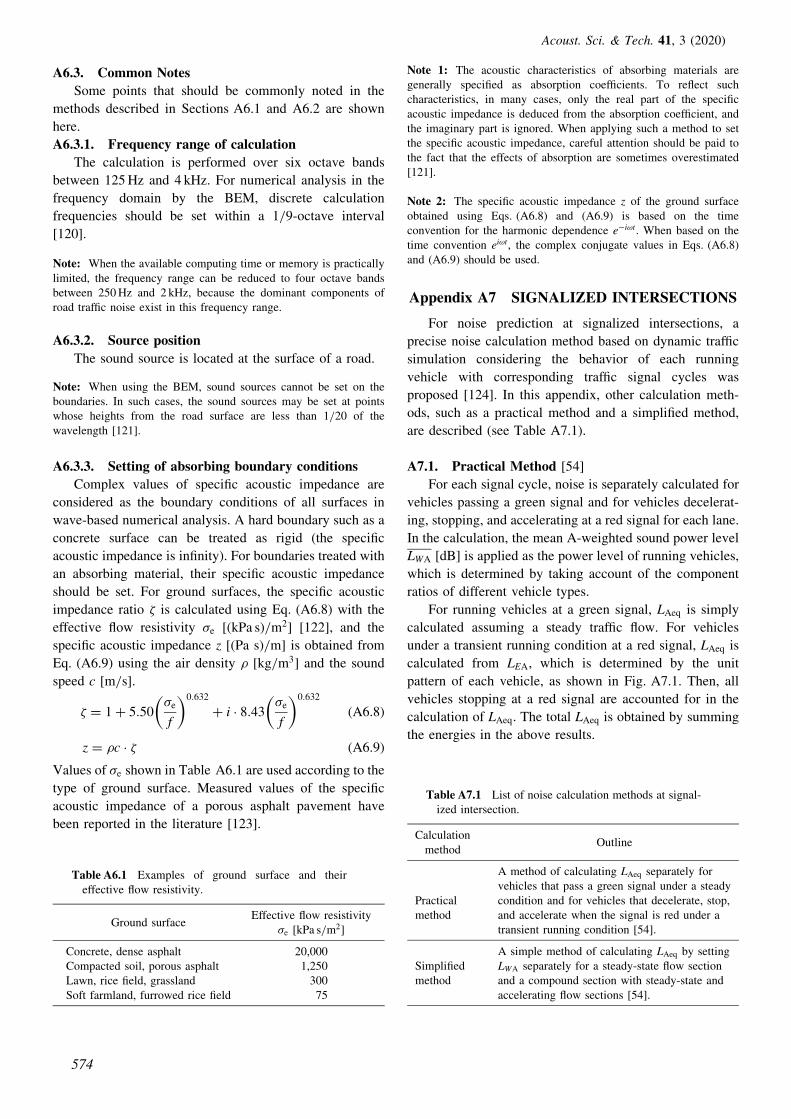
A6.3. Common Notes

Some points that should be commonly noted in the

methods described in Sections A6.1 and A6.2 are shown

here.

A6.3.1. Frequency range of calculation

The calculation is performed over six octave bands

between 125 Hz and 4 kHz. For numerical analysis in the

frequency domain by the BEM, discrete calculation

frequencies should be set within a 1/9-octave interval

[120].

Note: When the available computing time or memory is practicallylimited, the frequency range can be reduced to four octave bandsbetween 250 Hz and 2 kHz, because the dominant components ofroad traffic noise exist in this frequency range.

A6.3.2. Source position

The sound source is located at the surface of a road.

Note: When using the BEM, sound sources cannot be set on theboundaries. In such cases, the sound sources may be set at pointswhose heights from the road surface are less than 1/20 of thewavelength [121].

A6.3.3. Setting of absorbing boundary conditions

Complex values of specific acoustic impedance are

considered as the boundary conditions of all surfaces in

wave-based numerical analysis. A hard boundary such as a

concrete surface can be treated as rigid (the specific

acoustic impedance is infinity). For boundaries treated with

an absorbing material, their specific acoustic impedance

should be set. For ground surfaces, the specific acoustic

impedance ratio � is calculated using Eq. (A6.8) with the

effective flow resistivity �e [(kPa s)/m2] [122], and the

specific acoustic impedance z [(Pa s)/m] is obtained from

Eq. (A6.9) using the air density [kg/m3] and the sound

speed c [m/s].

� ¼ 1þ 5:50�e

f

� �0:632

þ i � 8:43�e

f

� �0:632

ðA6.8Þ

z ¼ c � � ðA6.9ÞValues of �e shown in Table A6.1 are used according to the

type of ground surface. Measured values of the specific

acoustic impedance of a porous asphalt pavement have

been reported in the literature [123].

Note 1: The acoustic characteristics of absorbing materials aregenerally specified as absorption coefficients. To reflect suchcharacteristics, in many cases, only the real part of the specificacoustic impedance is deduced from the absorption coefficient, andthe imaginary part is ignored. When applying such a method to setthe specific acoustic impedance, careful attention should be paid tothe fact that the effects of absorption are sometimes overestimated[121].

Note 2: The specific acoustic impedance z of the ground surfaceobtained using Eqs. (A6.8) and (A6.9) is based on the timeconvention for the harmonic dependence e�i!t. When based on thetime convention ei!t, the complex conjugate values in Eqs. (A6.8)and (A6.9) should be used.

Appendix A7 SIGNALIZED INTERSECTIONS

For noise prediction at signalized intersections, a

precise noise calculation method based on dynamic traffic

simulation considering the behavior of each running

vehicle with corresponding traffic signal cycles was

proposed [124]. In this appendix, other calculation meth-

ods, such as a practical method and a simplified method,

are described (see Table A7.1).

A7.1. Practical Method [54]

For each signal cycle, noise is separately calculated for

vehicles passing a green signal and for vehicles decelerat-

ing, stopping, and accelerating at a red signal for each lane.

In the calculation, the mean A-weighted sound power level

LWA [dB] is applied as the power level of running vehicles,

which is determined by taking account of the component

ratios of different vehicle types.

For running vehicles at a green signal, LAeq is simply

calculated assuming a steady traffic flow. For vehicles

under a transient running condition at a red signal, LAeq is

calculated from LEA, which is determined by the unit

pattern of each vehicle, as shown in Fig. A7.1. Then, all

vehicles stopping at a red signal are accounted for in the

calculation of LAeq. The total LAeq is obtained by summing

the energies in the above results.

Table A6.1 Examples of ground surface and theireffective flow resistivity.

Ground surfaceEffective flow resistivity

�e [kPa s/m2]

Concrete, dense asphalt 20,000Compacted soil, porous asphalt 1,250Lawn, rice field, grassland 300Soft farmland, furrowed rice field 75

Table A7.1 List of noise calculation methods at signal-ized intersection.

Calculationmethod

Outline

A method of calculating LAeq separately forvehicles that pass a green signal under a steady

Practical condition and for vehicles that decelerate, stop,method and accelerate when the signal is red under a

transient running condition [54].

A simple method of calculating LAeq by settingSimplified LWA separately for a steady-state flow sectionmethod and a compound section with steady-state and

accelerating flow sections [54].

Acoust. Sci. & Tech. 41, 3 (2020)

574

The A-weighted sound power levels near a signalized

intersection and the methods used to set various conditions

for the red-signal phase are given below.

A7.1.1. Sound power level near a signalized intersec-

tion


The acceleration running condition is defined as the

transitional state from stopping at a signalized intersection

to steady running. The speed range is from 1 to 60 km/h.

The constant power level (the value obtained when V ¼10 km/h is substituted into the equation for the deceleration

running condition) is applied to speeds of less than 1 km/h.

Acceleration at speeds exceeding 60 km/h is treated as a

steady running condition.


The deceleration running condition is defined as the

transitional state from steady running to stopping at a

signalized intersection. The speed range is more than

10 km/h. The sound power level at 10 km/h is applied at

speeds of less than 10 km/h.

A7.1.2. Method to set various conditions

(1) Mean A-weighted sound power level LWA

For the component ratio q of heavy vehicles in the two-

category classification, the mean A-weighted sound power

level LWA is calculated as

LWA ¼ aL þ b lgV þ 10 lgð1þ c � qÞ; ðA7.1Þ

where aL is a constant given in the equation of sound power

level for light vehicles [dB], b is a coefficient representing

the speed dependence, V is the running speed [km/h], and

c is the conversion coefficient of the sound power level

from a heavy vehicle to a light vehicle, which is calculated

using the following equation with the constant aH in the

equation for the sound power level for a heavy vehicle:

c ¼ 10ðaH�aLÞ=10 � 1: ðA7.2Þ

In the case of a dense asphalt pavement, the values to

be applied for aL, aH, and b are given in Table A7.2. In the

case of a porous asphalt pavement, the LWA can be

calculated using the values given in Table A4.1.

Note: The values for steady traffic flow sections in Table A4.1 areapplied to the deceleration running condition, whereas those for non-steady traffic flow sections are applied to the acceleration runningcondition.

(2) Setting of traffic volume

The number of vehicles that stop at a red signal during

one signal cycle NR [number of vehicles/cycle] is set as

NR ¼ NC �TR

TC

; ðA7.3Þ

where NC is the number of vehicles that pass through the

intersection in one signal cycle [number of vehicles/cycle],

TR is the duration of the red signal during one signal cycle

[s], and TC is the length of time of one signal cycle [s].

(3) Accelerations of vehicles

The accelerations while accelerating and decelerating

at signalized intersections are shown in Table A7.3.

(4) Mean headway and source positions of vehicles that

stop at red signal

The mean headway position d [m] of vehicles that stop

at a red signal is calculated as

d ¼ dL þ ðdH � dLÞ � q; ðA7.4Þ

where dL is the spacing of light vehicles that stop at a red

signal (¼ 6) [m], dH is the spacing of heavy vehicles that

stop at a red signal (¼ 12) [m], and q is the component

ratio of heavy vehicles. The source position of xn [m]

(distance from the stop line) of the nth vehicle that stops at

a red signal is calculated as

xn ¼ ðn� 0:5Þd: ðA7.5Þ

(5) Mean running speed when turning left/right

The mean running speed when turning left or right is

set to 20 km/h. However, speeds while accelerating to

20 km/h are calculated using the accelerations shown in

Table A7.3.

Fig. A7.1 Concept of time histories of LA for red-signalphase.

Table A7.2 Coefficients aL, aH, and b (dense asphaltpavement).

Running condition aL aH b

Acceleration 82.3 88.8 10Deceleration 45.8 53.2 30

Table A7.3 Accelerations while accelerating and decel-erating at signalized intersections.

Running condition Acceleration [m/s2]

Acceleration 1.0Deceleration �1:3


575

A7.2. Simplified Method [54]

The noise is calculated assuming that all vehicles

modeled in the practical method are represented by a single

vehicle with a constant speed along a steady-running

section. The road is divided into two sections. In one

section, all vehicles run steadily, and in the other, some

vehicles stop then accelerate at a red signal (a mixed

section with accelerating and steadily running vehicles).

The mean sound power level LWA of a vehicle is separately

given for each section. The concept of a mixed section with

accelerating and steadily running vehicles and a steady-

running section is illustrated in Fig. A7.2, and an illus-

tration of a unit pattern is shown in Fig. A7.3. LAeq;T is

calculated using Eq. (1.6) in Chapter 1 of the main body by

taking account of the traffic volume NT [vehicles] during

the time T [s] and LAE, which is obtained from the energy

integration of the unit pattern.

(1) Setting of mixed section and steady-running section

The length of the mixed section with accelerating and

steadily running vehicles is determined by summing the

section lengths lstop [m] and laccel [m], where lstop is the

distance from the front of the first vehicle to the rear of the

last vehicle when vehicles stop at a red signal and laccel is

the distance traveled by the first vehicle when it accelerates

to a constant speed after the signal turns green. The length

of each section is calculated as

lstop ¼ d � NR; ðA7.6Þ

laccel ¼v2

2aaccel

; ðA7.7Þ

where aaccel is the acceleration while accelerating [m/s2]

given in Table A7.3 and v is the speed in the steady-

running section [m/s]. A steady-running section is speci-

fied on both sides of the mixed section.

(2) Mean A-weighted sound power level LWA

The mean sound power level LWA for the steady-

running section is calculated using Eq. (A7.1). On the other

hand, LWA for the mixed section with accelerating and

steadily running vehicles is determined from the mean

sound power level LWA;B [dB] under the steady-running

condition (when the signal is green) and from LWA;R [dB]

under the accelerating condition, by averaging the power

using the component ratio of the traffic volume that passes

through the intersection at each signal phase. The mean

sound power level is calculated as

LWA ¼ 10 lgNR � 10LWA,R=10 þ ðNC � NRÞ � 10LWA,B=10

NC

;

ðA7.8Þwhere LWA;R is calculated by substituting the speed given

to vehicles in the steady-running section with the speed in

the equation for calculating the sound power level for

accelerating vehicles.

Appendix A8 ADVANCED CALCULATIONMETHOD FOR NOISE BEHINDBUILDING COMPLEX [125–127]

When the unit patterns must be calculated more

correctly for planning countermeasures against noise or

when the detailed diffraction and reflection by the sides of

the buildings must be considered, �LBB in Eq. (6.3) is

calculated using the following equation;

�LBB ¼ 10 lg

�a0 þ a1 �

�

�

þ a2

Xi

�i

��droad

dref;i

� �

þ a3 �1

n

Xnk¼1

0:251

1þ 0:522�k

� �

þ a4 � 10�0:0904��dSP

�;

ðA8.1Þ

where a0 ¼ 0:039, a1 ¼ 1:16, a2 ¼ 0:201, a3 ¼ 0:346, and

a4 ¼ 0:288.

In Eq. (A8.1), the term related to �=� indicates the

direct sound from the source to the prediction point. � and

� are the perspective angles [rad] from the prediction point

to a part of the target road of 10 m length where the sound

source S is the midpoint, as shown in Fig. A8.1, in the

Fig. A7.2 Concept of a compound section with accel-erating and steady running vehicles.

Fig. A7.3 Image of a unit pattern.

Acoust. Sci. & Tech. 41, 3 (2020)

576

cases with and without detached houses, respectively. The

term related toP

ið�i� �

droad

dref;iÞ indicates reflection sound

components. In this calculation method, the geometrical

reflections of the first and second orders from the detached

houses, which are located between the target road and the

prediction point and immediately behind the prediction

point, are considered. As shown in Fig. A8.2, �i is the

perspective angle [rad] from the first- or second-order

mirror point, P0 or P00, of the prediction point P to a portion

of the 10-m-long target road, droad is the perpendicular

distance between S and P, and dref;i is the perpendicular

distance between S and P0 or P00 (horizontal distance from

P0 or P00 to a foot on the perpendicular line at S).

The term related to 1n

Pnk¼1ð 0:251

1þ0:522�kÞ indicates the

diffracted sound from the source S to the prediction point P

via a vertex of a building O, as shown in Fig. A8.3. For the

calculation of this term, a number (n) of discrete source

points Sk are set on a part of the 10-m-long target road, and

the diffraction path difference SkOþ OP� SkP is calcu-

lated as �k [m]. When P is visible from Sk, the diffraction

sound is not calculated.

The term related to 10�0:0904��dSP indicates sounds other

than the direct, reflected, and single diffraction sounds. As

shown in Fig. 6.4, a 15-m-wide rectangular area is assumed

between S and P, and the density of the houses (the ratio of

the location area of the detached houses to the rectangular

area) � and the horizontal distance dSP between S and P are

calculated.

REFERENCES

Reference R1 NOISE REDUCTION EFFECTOF DOUBLE-LAYER POROUS ASPHALT

PAVEMENT

The double-layer porous asphalt pavement (DPA)

adopted in Japan is made of porous asphalt formed in

layers with the top layer having maximum chipping sizes

of 5–8 mm and thicknesses of 15–20 mm and the bottom

layer with a maximum chipping size of 13 mm and

thicknesses of 30–50 mm [128–130]. Figure R1.1 shows

the structures of DPA and a single-layer porous pavement

(PA).

(1) Noise reduction effect

Figure R1.2 shows the maximum A-weighted sound

pressure levels of a passenger car and a large-sized vehicle

measured on test tracks with DPA, PA, and a dense asphalt

pavement (DA) [131]. Figure R1.3 shows the noise

reduction effect of DPA, which was calculated using

the curves representing regression equations given in

Fig. R1.2. It can be seen that the A-weighted sound

pressure level on DPA decreases by 5–10 dB compared

with that on DA and by 4–6 dB compared with that on PA.

(2) Frequency characteristics of running noise

Figure R1.4 shows the maximum A-weighted sound

pressure levels in 1/3 octave bands on DPA, PA, and DA.

P

φ

P

SΦ

S

5m

d road

5m 5m5m

O

d road

O

Fig. A8.1 Perspective angles to the road, � and �, inthe cases without and with detached houses, respec-tively.

P

S

P’

S

P

P’

1st reflection

d ref , i

d road

d ref , i

d road

d road

d ref , i

θ i

θ i

2nd reflection

P

P’’

S

P’

θ i

5m 5m

P’

( )d roadd ref , iθ i

Traffic laneTraffic lane

Traffic lane

O O

O

S

PP’’ P’

( )d roadd ref , iθ i

5m 5m

Traffic lane

O

5m 5m5m 5m

Fig. A8.2 Perpendicular distance from P to S, droad, andperspective angle from mirror points of the receivers tothe source �i and the perpendicular distance dref;i.

P

Sk OS

Traffic lane5m 5m

Fig. A8.3 First-order diffraction sound with the vertexof the building as its diffraction point.


577

These data represent the sound spectra of the noise of

vehicles running at a constant speed of 60 km/h measured

on each pavement type (see Fig. R1.2). The sound pressure

levels on DPA at a frequency over 500 Hz are much lower

than those on DA. Moreover, the sound pressure levels of

DPA in the frequency range from 200 Hz to 1 kHz are

lower than those of PA.

(3) Aging variation in noise reduction effect

Aging variation in the noise reduction effect of DPA

was measured on general roads [130,132]. According to

these reports, the aging variation in the noise reduction

effect of DPA is similar to that of PA.

Reference R2 SOUND PROPAGATIONAROUND BARRIERS WITH OVERHANGS

AND EDGE-MODIFIED BARRIERS

To reduce diffracted noise more efficiently than by

using a standard simple barrier, edge-modified barriers or

barriers with overhangs are sometimes built along roads. In

this reference, methods for calculating sound propagation

around these barriers are described. Here, a barrier with its

top part simply folded is called a barrier with an overhang,

and a barrier with acoustic devices at the top edge is called

an edge-modified barrier.

Equations obtained through experiments have been

reported for the five types of barrier shown in Fig. R2.1

[133]. For other types of barrier including newly developed

ones, it is necessary to derive similar equations through

scale-model experiments or full-scale experiments.

The correction for diffraction around edge-modified

barriers and barriers with overhangs shown in Fig. R2.1 is

calculated using the following equations for each corre-

φ 5～8mm top

φ 13mm top

1515–20mm20mm

3030–50mm50mm

Double-layer porous asphalt pavement

φ 13mm top 4040–50mm50mm

Porous asphalt pavement

Fig. R1.1 Double- and single-layer porous asphalt pavements.

50

60

70

80

90

100

L A,F

max

[dB

]


Passenger car

Dense asphaltPorous asphaltDouble-layer porous asphalt

Dense: LA,Fmax = 11.9 + 32.2 lg VPorous: LA,Fmax = 27.5 + 22.7 lg VDouble-layer porous: LA,Fmax = 20.2 + 23.3 lg V

50

60

70

80

90

100

0 20 40 60 80 100 120

0 20 40 60 80 100 120

L A,F

max

[dB

]


Large-sized vehicle


Dense: LA,Fmax = 25.3 + 28.2 lg VPorous: LA,Fmax = 32.9 + 22.8 lg VDouble-layer porous: LA,Fmax = 26.0 + 24.6 lg V

Fig. R1.2 A-weighted sound pressure levels for differ-ent types of pavement.

0

5

10

15

0 20 40 60 80 100 120

Noi

se re

duct

ion

effe

ct [d

B]


DPA / DA, Passenger carDPA / DA, Large-sized vehicleDPA / PA, Passenger carDPA / PA, Large-sized vehicle

Fig. R1.3 Noise reduction by double-layer porous as-phalt pavement.

Acoust. Sci. & Tech. 41, 3 (2020)

578

sponding situation regarding the positions of source point S

and prediction point P shown in Fig. R2.2.

(For barriers with overhangs)

�Ldif,ob ¼ �Ldif,hb þ Cdif,ob ðR2.1Þ

(For edge-modified barriers)

�Ldif,emb ¼ �Ldif,hb þ Cdif,emb ðR2.2Þ

Here�Ldif,ob and�Ldif,emb [dB] are the correction terms for

diffraction around the barrier with an overhang and the

edge-modified barrier; �Ldif,hb [dB] is the correction term

for a hypothetical simple barrier whose top edge corre-

sponds to the intersection O of two straight lines SX and

PY: a line through the point source and the source-side

diffraction point, and a line through the prediction point

and the receiver-side diffraction point, as shown in

Fig. 3.8; and Cdif,ob and Cdif,emb are the correction terms

for the overhang and acoustic device, respectively.

When the prediction point P is located in Region 1 or

Region 2 as shown in Fig. R2.2, Cdif,ob and Cdif,emb are

calculated using the following equations. Cdif,ob and Cdif,emb

are 0 when P is in Region 3.

Cdif,ob

Cdif,emb

!¼�A� B lg �þ CRegion2 � � 1

�C � D sinh�1 �E þ CRegion2 0 � � < 1

(

ðR2.3Þ

CRegion2 ¼max½F lg � þ G; 0 P 2 Region 2

0 P 2 Region 1

(ðR2.4Þ

Here � is the path difference for the hypothetical simple

barrier [m], � is the angle between XY and XP in Fig. R2.2

[deg], and max½a; b gives the larger value of a and b.

Values for coefficients A to G are given in Table R2.1.

Note 1: Because the equations for Cdif,ob and Cdif,emb are derivedfrom the experimental results with absorptive barriers, they shouldnot be corrected with the correction term Cdif,abs for the absorptioneffect of the standard metallic absorptive-type barrier, defined asEq. (3.6).

Note 2: The prediction accuracy for barriers with overhangs inRegion 3 has not been verified.

Note 3: Procedures for calculating the A-weighted sound pressurelevel using the correction term �Ldif,ob or �Ldif,emb in wave-basednumerical analysis are shown in Ref. [134].

20

30

40

50

60

70

80

90A

-wei

ghte

d ba

nd so

und

pres

sure

leve

l[dB

]

Frequency [Hz]

Passenger car, 60 km/h


20

30

40

50

60

70

80

90

63 125 250 500 1k 2k 4k 8k

63 125 250 500 1k 2k 4k 8k

A-w

eigh

ted

band

soun

d pr

essu

re le

vel[

dB]

Frequency [Hz]

Large-sized vehicle, 60 km/h


Fig. R1.4 Frequency characteristics of the maximumA-weighted sound pressure levels in 1/3 octave bandson double-layer porous asphalt pavement.

(1) (2) (3) (4) (5)

3.0 m

1.5 m

1.15 m

0.36 m

2.0 m

1.0 m

3.0 m 5.0 m

Fig. R2.1 Types of edge-modified barriers and barriers with overhangs: (1) large branch type, (2) standard branch type,(3) branch type for bridges, (4) L-shaped (3 m), and (5) L-shaped (5 m). Broken lines indicate absorption surfaces.


579

Reference R3 EXPRESSIONS FOR LAeq

UNDER SIMPLE ROAD CONDITIONS

If a road is straight and infinitely long and the sound

diffraction and the effects of the ground are ignored,

LAeq can be determined using an analytical solution

[135].

LAeq;T can be calculated using the following equation

involving the single-event sound exposure level LEA [dB]

and the traffic volume NT [number of vehicles] passing a

prediction point during the time T [s]:

LAeq;T ¼ LEA þ 10 lgNT

TðR3.1Þ

When an omnidirectional point source with the A-weighted

sound power level LWA [dB] moves along a straight road

of infinite length at a constant speed V [km/h], LAE at the

distance l [m] from the lane can be analytically derived

from the following equation obtained by applying the

inverse-square law in a hemi-free field and integrating over

time up to infinity:

LAE ¼ LWA þ 10 lg3:6

2lV

� �: ðR3.2Þ

Then, LAeq;T can be calculated as

LAeq;T ¼ LWA � 10 lg l� 10 lgV þ 10 lgNT þ 10 lg3:6

2T:

ðR3.3ÞSince LWA is given for each vehicle category, LAeq;T for the

entire traffic is calculated by the energy summation of the

obtained results for respective vehicle types.

Reference R4 STUDY OF PREDICTIONACCURACY

The calculation models of sound power levels of road

vehicles and calculation methods of sound propagation

were updated so that the calculated value becomes more

accurate to the measured road traffic noise. Since many

assumptions are included in setting the power level of

running-vehicle noise and in simplifying the calculation of

noise propagation in ASJ RTN-Model 2018, it is necessary

to examine the prediction accuracy of this model.

Here, we describe the results of an investigation in

which actual measurement values are compared with

values predicted using the previous model. In addition, it

is necessary to note that several types of uncertainty are

included in the actual measurement values. We also

(2)

S

P

22

Region 3

Region 1X Y

(1)

S

P

22 θ

Region 3

Region 1

Region 2X Y

(3)

S

P

22

Region 3

Region 1

Region 2X Y

θ

Fig. R2.2 Definitions of regions 1 to 3: (1) large and standard branch-type barriers, (2) branch-type barriers for bridges, and(3) L-shaped barriers.

Table R2.1 Coefficients for the correction terms Cdif,ob and Cdif,emb.

Pavement Barrier A B C D E F GApplicablerange of �

Large branch type5.0 3.0 2.1 3.29 0.414

5.31 �1:4 0.11–10

Standard branch type 1.88 �0:3 0.0003–11

Dense Branch type for3.5 5.0 0.0 3.97 0.600 — — 0.0004–3.5

asphalt bridges

L-shaped (3 m)1.0 5.0 0.0 1.14 0.414

2.66 0.7 0.02–20

L-shaped (5 m) 3.66 1.4 0.08–34

Large branch type3.7 3.0 2.1 1.82 0.414

4.42 �1:6 0.11–10

Standard branch type 1.65 0.1 0.0003–11

Porous Branch type for2.5 4.5 0.0 2.84 0.600 — — 0.0004–3.5

asphalt bridges

L-shaped (3 m)1.0 3.5 0.0 1.14 0.414

2.30 1.2 0.02–20

L-shaped (5 m) 3.02 1.7 0.08–34

Acoust. Sci. & Tech. 41, 3 (2020)

580

examine the causes of errors that are likely to be significant

when considering the prediction accuracy of ASJ RTN-

Model 2018.

R4.1. Relationship between Predicted and Measured

Values at General Road Section [136]

R4.1.1. Actual measurement data used in this exami-

nation

The actual measurement data were obtained at straight

sections of general roads in fiscal year 2013 based on the

manual of constant monitoring of motor vehicle traffic

noise [137] by the Japanese Ministry of the Environment.

The measurements were in accordance with JIS

Z8731:1999, which is almost identical to ISO 1996-

1:2016. The measurement conditions of these data are as

follows.

(1) Noise levels considered

LAeq and LANðLA5; LA10; LA50; LA90;LA95Þ. The measure-

ment duration was 10 min, and multiple measurement were

performed over 24 h at each location.

(2) Measurement point

1.2 m above the ground on a public/private boundary.

The selected measurement points were away from juxta-

posed roads or road intersections, and without obstructions

or glass ground in the sound propagation path. The number

of lanes was from 1 to 4.

(3) Traffic volume

The traffic volume was determined with the three-

category or two-category vehicle classification for each

direction. The number of motorcycles was also counted

separately. The traffic volumes of the target roads were less

than 4,500 per hour, and the ratio of heavy vehicles varied

widely (from 0% to 100%).

(4) Running speed

Obtained for both directions. The measurement data of

traffic flow with running speed less than 40 km/h were

excluded from the examination.

R4.1.2. Calculation

The predicted values were obtained using the calcu-

lation procedures described in Reference R3; the A-

weighted sound power levels LWA on a dense asphalt

pavement in a steady traffic flow section were used.

Multiple lanes of traffic traveling in the same direction

were combined into a hypothetical single lane at the center

of the traffic stream.

R4.1.3. Comparison of predicted and measured values

The relationship between the predicted and actual

measurement values for daytime (6:00–22:00) and night-

time (22:00–6:00) is shown in Fig. R4.1. In the scatter

diagrams, the line where the predicted and measured values

coincide and its 3 dB range are also shown. The correlation

coefficients were 0.81 for daytime and 0.85 for nighttime.

The mean differences between the predicted and measured

values (�, predicted LAeq minus actual measurement

values) were +0.4 and �0:8 dB for daytime and nighttime,

respectively, indicating excellent agreement between the

two values. For daytime, 87% of the prediction was

included within the �3 dB range, where 78% was included

for nighttime.

R4.2. Relationship between Predicted and Measured

Values on Roadside of Expressway [138]

R4.2.1. Actual measurement data used in this exami-

nation

The actual measurement data were obtained at express-

ways with bank and cut road structures in fiscal years from

2014 to 2018. A summary of seven selected measurement

points is shown in Table R4.1.

N = 1354, Δ = 0.4, σ = 2.2r = 0.81

N = 1346, Δ = -0.8, σ = 2.6r = 0.85

Fig. R4.1 Relationship between predicted and mea-sured LAeq at flat and straight general road section.


581

(1) Noise levels considered

LAeq and LA95 (the lower limit of the 90% percentile

range). The measurement duration was 2 h for road 1–6,

while the duration was 15 min for road 7.

(2) Measurement point

The roadside measurement points were 1.2 m above the

ground surface. The reference measurement points for the

bank roads (roads 1–6) were 1.2–2.8 m above the road

surface at a distance of 7.5 m from the center of the closest

cruising lane. For the cut road (road 7), the reference point

was 3.0 m above the 2.0-m-high noise barrier on the top of

the slope.

(3) Traffic volume

The traffic volume for the bank roads (roads 1–6) was

determined with the three-category vehicle classification

for each direction and each lane. Buses and motorcycles

were separately counted. The traffic volume for the cut

road (road 7) was counted by traffic counter with the two-

category vehicle classification for each direction and each

lane.

The traffic volumes of the target roads (roads 1–7) were

from 800 to 4,000 per hour, and the ratio of heavy vehicles

were varied from 17% to 32%.

(4) Running speed

For the bank roads (roads 1–6), the running speed of

traffic was determined for each direction, each lane, and

each type of vehicle by visual measurements. For the cut

road (road 7), the running speed measured by the traffic

counter for each direction and each lane was used. The

average running speeds of the target traffic were from 80 to

110 km/h.

R4.2.2. Calculation

The predicted values were obtained by the calculation

procedure described in Subsection 1.3.2 using actual

measured traffic conditions.

The calculation position for each lane was located at

the center of the lane. The corrections for the diffraction on

the top of the slope of the bank structures were calculated

by the method for the wedge with an opening angle. The

correction for the noise barrier was calculated by the

method for the knife wedge. The correction for the

absorptive barrier was also involved. Regarding the

correction of the ground effect for the slope surface, the

coefficients for loose soil were used, while the correction

was set to 0 dB for the ground of the measurement side since

the surfaces were covered by an asphalt pavement. The

correction for atmospheric absorption was also involved.

Since the roadside measurement point of the cut road

(road 7) was behind a noise barrier, two types of calculation

were performed with and without taking account of the

reflection from the ground (see Note 5 in Section 3.3).

R4.2.3. Comparison of predicted and measured values

The relationship between the predicted and actual

measurement values for each road structure is shown in

Fig. R4.2. For the bank roads, the reflection of the ground

was considered. Since the measured LAeq were at least

10 dB higher than LA95, no correction of background noise

was performed.

For the bank roads, the predicted values corresponded

to within 3 dB of the measured values. With regard to the

porous asphalt pavements, the mean differences between

the predicted and measured values (�, predicted value of

LAeq minus actual measurement values) were +0.6 and

+0.8 dB at the reference and roadside points, respectively.

The mean differences for the KOUKINOU II pavement,

even though there was only one case, were +0.8 dB at the

reference and +1.5 dB at the roadside points.

For the cut road, the mean differences between the

predicted and measured values at the roadside point were

+0.3 and �1:6 dB in the case with and without taking

account of the ground reflection, respectively. The pre-

diction considering the ground reflection showed better

agreement with the actual measurement.

R4.3. Accuracy Verification of Practical Calculation

Method for Areas behind Buildings [139]

In ASJ RTN-Model 2018, a practical calculation

method is provided for predicting noise behind a dense

building complex (Section 6.2). Two types of verification

of the predicted and measured values were explained in

this section: the correspondence of A-weighted sound

pressure level using test vehicles and the correspondence of

Table R4.1 Summary of the measured data used for the examination.

Structure Pavement Number of measurement pointsNoise barriers

type Type Age Reference Roadside

1 bank porous 8.0 1 1 none2 bank porous 6.3 1 1 none3 bank porous 7.3 1 1 none4 bank porous 8.3 1 1 none5 bank porous 0.5 1 1 none6 bank KOUKINOU II 1.3 1 1 none7 cut porous 3.0 1 2 2 m height

Acoust. Sci. & Tech. 41, 3 (2020)

582

A-weighted equivalent continuous sound pressure levels

using road traffic census data.

R4.3.1. Verification using measurement value using

test vehicles

Unit patterns in areas behind buildings were verified for

the situation in which test vehicles run on a plane road or a

cut road at a steady speed.

(1) In a residential area facing a plane road

The correspondence between the prediction and actual

measurement values was examined in areas behind build-

ings facing a plane road. The test vehicles were independ-

ently passing by at a constant speed. The running speed and

the A-weighted sound power level of the test passenger

cars were estimated to be 35.6 km/h and 92.5 dB, respec-

tively. Those of the test motorcycles were estimated to be

46.1 km/h and 97.4 dB, respectively.

The prediction and actual measurement values of the

maximum A-weighted sound pressure level LA,Fmax at 9

points behind the buildings are shown in Fig. R4.3.

Regardless of vehicle type, the differences between the

prediction and actual measurement values were within

approximately �3 dB.

(2) In a residential area facing a cut road

The correspondence in areas behind buildings facing a

cut road was examined. A test vehicle (passenger car) was

independently passing by at a constant speed of 41.9 km/h,

and its A-weighted sound power level was estimated to be

98.6 dB.

The prediction and actual measurement values of the

maximum A-weighted sound pressure level LA,Fmax at 5 out

of 45 predicted points behind the buildings, where the

diffraction on the top of the slope would be considered, are

shown in Fig. R4.4. The calculations were performed with

the correction of the diffraction on the top of the slope

(shown as filled circles) and without correction in which

the road surface level was equal to the ground of the

residences (shown as open circles). The results demonstrate

that the practical calculation method can be applied to

areas facing a cut road with correction of the diffraction on

the top of the slope and the attenuation by buildings. The

differences between the prediction and actual measurement

values were within �3 dB.

R4.3.2. Verification using road traffic census data

Equivalent noise levels were calculated in areas behind

buildings facing plane roads, hereinafter called as Road-A

40

45

50

55

60

65

70

75

80

Pre

dict

edL A

eq[d

B]

Measured LAeq [dB]

Porous (Reference)Porous (Roadside)KOUKINOU II (Reference)KOUKINOU II (Roadside)

PorousReference :

Δ = 0.6 dBσ = 1.70 dB

N = 5Roadside :

Δ = 0.8 dB σ = 2.10 dB

KOUKINOU IIReference :

Δ = 0.8 dB, N = 1Roadside :

40

45

50

55

60

65

70

75

80

40 45 50 55 60 65 70 75 80

40 45 50 55 60 65 70 75 80

Pre

dict

edL A

eq[d

B]

Measured LAeq [dB]

Reference pointRoadside points (with reflection)Roadside points (without reflection)

Reference point

Roadside points (with reflection)Δ = 0.3 dB, σ = 0.14 dB, N = 2

Roadside points (without

Fig. R4.2 Relationship between predicted and mea-sured LAeq on the roadside of expressways.

Fig. R4.3 Relationship between predicted and mea-sured values of maximum A-weighted sound pressurelevels behind buildings facing a plane road.


583

and Road-B, to examine the prediction accuracy and to

develop a noise map. In this calculation, road traffic census

data were used for estimating the traffic conditions. As the

results of the estimations for road-A, the hourly traffic

volume consisted of 3,370 small-sized vehicles and 996

large-sized vehicles, and the average running speed was

36.7 km/h. The A-weighted sound power levels of the

vehicles were determined to be 92.7 dB for the small-sized

vehicles and 100.1 dB for the large-sized vehicles on the

assumption that the vehicles were running at a steady

speed, since the measurement point was distant from the

signalized intersections and its traffic was steady. As the

results of the estimations for Road-B, the hourly traffic

volumes consisted of 768 small-sized vehicles and 64

large-sized vehicles, and the average passage speed was

19.9 km/h. The A-weighted sound power levels were

determined to be 95.3 dB for the small-sized vehicles and

101.8 dB for the large-sized vehicles on the assumption

that the vehicles are not running at a steady speed owing to

the traffic signals along Road-B.

Figure R4.5 shows that the differences between the

prediction and actual measurement values at the intended

Road-A and Road-B were within approximately �3 and

�5 dB, respectively.

R4.4. Causes of Errors in ASJ RTN-Model 2018

R4.4.1. Setting of hypothetical traffic lanes

In ASJ RTN-Model 2018, it is permitted to combine

two or more lanes into a single hypothetical lane for

simplicity of the calculation. According to a previous

investigation [140], the difference in LAeq caused by

combining the lanes into a single lane was less than 1 dB,

even in the case of a road with eight lanes, if the distance

from the center of the nearest lane to the receiver was 5 m

or more. However, the error increases markedly when the

distance to the receiver is less than 5 m. Thus, when noise

is predicted in the vicinity of roads with multiple lanes, it is

recommended to increase the number of hypothetical lanes.

R4.4.2. Road traffic conditions

(1) Variations of vehicle running speed and sound

power level

In ASJ RTN-Model 2018, the sound power level of a

road vehicle is calculated under the assumption that all

vehicles classified in each category run at the same speed

(i.e., at the mean speed of all vehicles). According to the

results of examination from a stochastic viewpoint [141],

the change in LAeq due to the variation of running speed is

extremely small. Furthermore, the change in LAeq is 1 dB or

less if the standard deviation of the power level is 3 dB or

less.

(2) Vehicle classification

In ASJ RTN-Model 2018, two types of vehicle

classification are applied: the three-category classification

(small-sized vehicles, medium-sized vehicles, and large-

sized vehicles) and the two-category classification (light

vehicles and heavy vehicles). It is preferable to apply the

former classification. However, even when the two-cat-

egory classification is applied, the errors in the predicted

values caused by replacing the two-category classification

with the three-category classification are 1 dB or less if the

ratio of medium-sized vehicles to large-sized vehicles

ranges from 10 to 80% [136].

R4.4.3. Range of unit pattern calculation

In the basic scheme of ASJ RTN-Model 2018, point

sources are discretely set on lanes to obtain the unit pattern

Fig. R4.4 Relationship between predicted and mea-sured values of maximum A-weighted sound pressurelevels behind buildings facing a cut road.

Fig. R4.5 Relationship between predicted and mea-sured LAeq using road traffic census data.

Acoust. Sci. & Tech. 41, 3 (2020)

584

at the receiver, and then LAeq is calculated. In this case, it

is necessary to determine the range over which the point

sources must be arranged. In other words, the range of the

unit pattern calculation is essential. In Ref. [140], on the

basis of the calculated unit patterns for flat roads,

interchange sections, and the areas surrounding a tunnel

portal, the errors in LAeq caused by removing the low-level

portions of the unit pattern (i.e., the portions where the

A-weighted sound pressure level is 5, 10, or 15 dB smaller

than the maximum) are examined. As a result, it was found

that the errors are approximately 1 dB or less even when

the low-level portions 10 dB below the maximum for flat

roads and for interchange sections or 15 dB below the

maximum for areas surrounding a tunnel portal are

removed. However, since LAeq strongly depends on the

energy integration over the entire unit pattern, it is

necessary to note that a significant error may occur owing

to the lack of consecutive portions of the unit pattern.

Hence, it is necessary to avoid the excessive removal of

portions, even if the A-weighted sound pressure levels are

sufficiently smaller than the maximum.

R4.4.4. Problems encountered in actual measurements

In addition to considering problems in the prediction

calculation, it is necessary to consider the causes of

uncertainties in the actual measurements of road traffic

noise. Typical causes of uncertainties are discussed below.

It is also necessary to consider the measurement duration

necessary to stabilize the values of LAeq statistically.

(1) Effects of meteorological factors

When sounds propagate outdoors, the effects of the

temperature profile and wind in the atmosphere appear as

propagation distance increases. Attenuation may also occur

owing to atmospheric absorption, which depends on

atmospheric temperature and humidity. Among these

effects, the wind and temperature profiles are extremely

complicated, and it is still difficult to take these effects into

account in practical noise prediction. Thus, only the

variation of road traffic noise as affected by wind, which

is based on actual measurement results, is introduced in

ASJ RTN-Model 2018, as described in Section 3.6. Sound

propagation may also be affected by the temperature

gradient. However, its effect can be ignored for propaga-

tion distances of up to approximately 200 m, unless

extreme temperature inversion occurs. For attenuation

caused by atmospheric absorption, a comparatively precise

calculation is available, as described in Section 3.4.

(2) Influence of background noise

In the measurement of road traffic noise, other types of

noise (background noise) always affect the measurement

results to some extent. In particular, the effect of back-

ground noise is larger when the receivers are far from the

road or noise reduction measures such as noise barriers are

provided. Although several methods of estimating the

degree of background noise have already been investigated,

an approximate background noise level can be estimated by

simultaneously measuring the percentile level, LA90 or

LA95, along with LAeq.

(3) Effect of other factors

Since road traffic noise may be measured under

circumstances that are not taken into account in the

prediction, not only the causes described above but also

various other causes of errors must be considered, for

instance, errors caused by traffic flow conditions that are

different from those set in the prediction or a difference in

the performance of noise reduction measures such as noise

barriers due to their installation condition. For a porous

asphalt pavement, although the noise reduction effect and

its change with time after the installation are taken into

account in ASJ RTN-Model 2018, the deterioration of its

performance caused by the blockage of air pores may

significantly depend on its location. In the case of a

viaduct, not only structure-borne noise, which is already

taken into consideration in ASJ RTN-Model 2018, but also

noise from the expansion joints of the road may often be

included in actual measurement values.

REFERENCES

[1] S. Sakamoto, ‘‘Roles achieved by Research Committee onRoad Traffic Noise and future subjects to be solved by theCommittee,’’ Proc. Autumn Meet. Acoust. Soc. Jpn.,pp. 1543–1546 (2012) (in Japanese).

[2] K. Ishii, ‘‘Prediction of road traffic noise (part 1), method ofpractical calculation,’’ J. Acoust. Soc. Jpn. (J), 31, 507–517(1975) (in Japanese).

[3] K. Ikegaya, ‘‘Mathematical models and estimation forpredicting the road traffic noise,’’ J. Acoust. Soc. Jpn. (J),31, 559–565 (1975) (in Japanese).

[4] K. Ishii, ‘‘Prediction of road traffic noise,’’ J. Acoust. Soc. Jpn.(J), 33, 426–430 (1977) (in Japanese).

[5] M. Sasaki and M. Yamashita, ‘‘Discussion on the predictionmethod of traffic noise in the vicinity of the road tunnel,’’ J.Acoust. Soc. Jpn. (J), 40, 554–558 (1984) (in Japanese).

[6] M. Sasaki and M. Yamashita, ‘‘Discussion on the predictionmethod of traffic noise in the vicinity of road interchange,’’ J.Acoust. Soc. Jpn. (J), 40, 638–643 (1984) (in Japanese).

[7] H. Tachibana, ‘‘Energy-base prediction method of road trafficnoise from general types of roads (Report from ResearchCommittee of Road Traffic Noise in Acoustical Society ofJapan),’’ J. Acoust. Soc. Jpn. (J), 50, 227–252 (1994) (inJapanese).

[8] Research Committee of Road Traffic Noise in AcousticalSociety of Japan, ‘‘ASJ Prediction Model 1998 for RoadTraffic Noise — Report from Research Committee of RoadTraffic Noise in Acoustical Society of Japan —,’’ J. Acoust.Soc. Jpn. (J), 55, 281–324 (1999) (in Japanese).

[9] Research Committee of Road Traffic Noise in the AcousticalSociety of Japan (Chairman: H. Tachibana), ‘‘Road trafficnoise prediction model ‘ASJ RTN-Model 2003’ proposed bythe Acoustical Society of Japan,’’ J. Acoust. Soc. Jpn. (J), 60,192–241 (2004) (in Japanese).

[10] K. Yamamoto, ‘‘Road traffic noise prediction model ‘‘ASJRTN-Model 2008’’: Report of the Research Committee on


585

Road Traffic Noise,’’ Acoust. Sci. & Tech., 31, 2–55 (2010).[11] S. Sakamoto, ‘‘Road traffic noise prediction model ‘‘ASJ

RTN-Model 2013’’: Report of the Research Committee onRoad Traffic Noise,’’ Acoust. Sci. & Tech., 36, 49–108 (2015).

[12] National Institute for Land and Infrastructure Management inthe Ministry of Land, Infrastructure, Transport and Tourismof Japan, ‘‘Environment Impact Assessment Technique forRoad Project 4. Noise 4.1 Noise Caused by Road Traffic(Revision of FY 2014),’’ Technical Note of National Institutefor Land and Infrastructure Management, No. 842 (2015) (inJapanese).

[13] Highway Environment Research Institute, Technical Methodfor Environmental Impact Assessment of Roads, AdditionalVersion No. 2 (Maruzen, Tokyo, 2007) (in Japanese).

[14] S. Sakamoto, Y. Okada, A. Fukushima, T. Matsumoto, K.Anai and T. Tajika, ‘‘Discussions on establishing ASJ RTN-Model 2018,’’ Proc. Spring Meet. Acoust. Soc. Jpn.,pp. 1449–1450 (2018) (in Japanese).

[15] Y. Okada, T. Ichikawa, K. Yoshihisa, T. Uemura, M.Yonemura, H. Lee, S. Sakamoto and K. Yamauchi, ‘‘Soundpower level of road vehicles running on dense asphaltpavement at various sites in Japan,’’ Acoust. Soc. & Tech., 41,598–606 (2020).

[16] K. Tsukui, Y. Okada, K. Yoshihisa and Y. Oshino, ‘‘Measure-ment results of sound power levels for motorcycles and theircalculation model,’’ Tech. Rep. Noise and Vib. Acoust. Soc.Jpn., N-2009-21 (2009) (in Japanese).

[17] A. Fukushima, T. Itiki, T. Ohta, O. Funahashi, T. Ookura, H.Iwabuki and H. Kaneshige, ‘‘Sound power level and powerspectrum of road vehicles running on expressways,’’ Tech.Rep. Noise and Vib. Acoust. Soc. Jpn., N-2019-14 (2019) (inJapanese).

[18] Y. Oshino and H. Tachibana, ‘‘Prediction of road traffic noisetaking account of transient running condition of vehicles,’’Proc. Inter-noise 93, pp. 629–632 (1993).

[19] T. Tajika, Y. Oshino and H. Tachibana, ‘‘A study oncorrection to sound power levels of vehicles at a road withslope — Part 2. Calculation of the correction value consider-ing LAE —,’’ Tech. Rep. Noise and Vib. Acoust. Soc. Jpn., N-2004-18 (2004) (in Japanese).

[20] K. Tsukui, Y. Oshino and H. Tachibana, ‘‘Road traffic noisesimulation model taking account of vehicle noise directiv-ities,’’ Proc. Inter-noise 98, pp. 1633–1636 (1998).

[21] Y. Mori, A. Fukushima, K. Uesaka and H. Ohnishi, ‘‘Noisedirectivity of vehicles on actual road,’’ Proc. Inter-noise 99,pp. 209–212 (1999).

[22] T. Matsumoto, ‘‘Scale model experiments for prediction ofroad traffic noise,’’ J. Acoust. Soc. Jpn. (J), 63, 537–542(2007) (in Japanese).

[23] Z. Maekawa, ‘‘Noise reduction by barriers,’’ Appl. Acoust., 1,157–173 (1968).

[24] K. Yamamoto and K. Takagi, ‘‘Expressions of Maekawa’schart for computation,’’ Appl. Acoust., 37, 75–82 (1992).

[25] A. Fukushima, S. Sakamoto and Y. Yasuda, ‘‘Practicalcalculation method of noise reduction by thick barrier,’’ Tech.Rep. Noise and Vib. Acoust. Soc. Jpn., N-2018-35 (2018) (inJapanese).

[26] A. Fukushima, S. Sakamoto, Y. Yasuda and T. Yokota,‘‘Road traffic noise prediction model ‘‘ASJ RTN-Model2018’’ — Calculation model of sound propagation —,’’ Proc.Spring Meet. Acoust. Soc. Jpn., pp. 1397–1400 (2019) (inJapanese).

[27] T. Okubo and A. Fukushima, ‘‘Calculation method forabsorbing effect of absorptive noise barrier in road trafficnoise prediction,’’ Proc. Spring Meet. Acoust. Soc. Jpn.,

pp. 1123–1126 (2014) (in Japanese).[28] K. Takagi, R. Hotta and K. Yamamoto, ‘‘A simple method for

the calculation of noise attenuation by a finite length barrier,’’Appl. Acoust., 43, 353–365 (1994).

[29] K. Takagi, Y. Park, R. Hotta and K. Yamamoto, ‘‘Comparisonof simple prediction method for noise reduction by doublebarriers,’’ Proc. Inter-noise 96, pp. 779–782 (1996).

[30] K. Uesaka, H. Ohnishi, T. Miyake, K. Yamamoto and K.Takagi, ‘‘Calculation method for sound attenuation by multi-ple barriers with wide intervals,’’ Proc. Spring Meet. Acoust.Soc. Jpn., pp. 705–706 (1999) (in Japanese).

[31] A. Fukushima and T. Itiki, ‘‘Numerical analysis of diffractionsound field around anomalous double barriers and consid-eration of practical calculation model,’’ Tech. Rep. Noise andVib. Acoust. Soc. Jpn., N-2017-22 (2017) (in Japanese).

[32] S. Sakamoto, Y. Yasuda and A. Fukushima, ‘‘A study onpractical calculation method of diffraction field around thickbarrier,’’ Tech. Rep. Noise and Vib. Acoust. Soc. Jpn., N-2017-23 (2017) (in Japanese).

[33] A. Fukushima and S. Sakamoto, ‘‘Practical calculationmethod of noise reduction by overhanged barrier,’’ Tech.Rep. Noise and Vib. Acoust. Soc. Jpn., N-2019-12 (2019) (inJapanese).

[34] T. Okubo and K. Yamamoto, ‘‘Noise shielding efficiency ofbarriers with eaves against road traffic noise,’’ Proc. AutumnMeet. INCE/J, pp. 121–124 (2008) (in Japanese).

[35] T. Miyake, K. Uesaka, H. Ohnishi, K. Yamamoto and K.Takagi, ‘‘A study on expression of ground effect for vehiclenoise propagation,’’ Proc. Spring Meet. Acoust. Soc. Jpn.,pp. 725–726 (1998) (in Japanese).

[36] T. Yokota and T. Okubo, ‘‘Numerical experiments ofmeteorological effects on propagation of road traffic noise,’’Tech. Rep. Noise and Vib. Acoust. Soc. Jpn., N-2014-19(2014) (in Japanese).

[37] K. Yoshihisa, Y. Okada, T. Yokota and T. Iwase, ‘‘Exper-imental study on the effects of wind and the ground onhorizontal propagation of sound,’’ Proc. Inter-noise 2006,pp. 5540–5548 (2006).

[38] T. Yokota, T. Matsumoto and A. Fukushima, ‘‘Study on themeteorological effects on road traffic noise propagation:Numerical experiments on variations in ground attenuationand diffraction by a simple barrier due to wind effect,’’ Tech.Rep. Noise and Vib. Acoust. Soc. Jpn., N-2019-16 (2019) (inJapanese).

[39] K. Yamamoto and M. Yamashita, ‘‘A simple model forestimating excess attenuation of road traffic noise,’’ J. Acoust.Soc. Jpn. (E), 8, 13–22 (1987).

[40] A. Fukushima, T. Itiki, T. Ohta, T. Nakao, H. Iwabuki and T.Osafune, ‘‘Measurements of acoustic characteristics of drain-age asphalt and excess attenuation on sound propagation overthe surface,’’ Tech. Rep. Noise and Vib. Acoust. Soc. Jpn., N-2015-16 (2015) (in Japanese).

[41] T. Miyake, H. Toriumi and S. Suzuki, ‘‘Excess attenuation ofvehicle noise propagation over various grounds,’’ Proc.Autumn Meet. Acoust. Soc. Jpn., pp. 767–768 (2003) (inJapanese).

[42] K. Yamamoto, M. Yamashita and T. Mukai, ‘‘Revisedexpression of vehicle noise propagation over ground,’’ J.Acoust. Soc. Jpn. (E), 15, 233–241 (1994).

[43] K. Yoshihisa, T. Nasu, K. Takagi and H. Tachibana, ‘‘Effectof atmospheric absorption on road traffic noise propagation,’’Tech. Rep. Noise and Vib. Acoust. Soc. Jpn., N-1999-21(1999) (in Japanese).

[44] A. Fukushima and K. Yamamoto, ‘‘Calculation method ofnoise attenuation by barrier on the assumption of energetic

Acoust. Sci. & Tech. 41, 3 (2020)

586

reciprocity, and its applications,’’ Tech. Rep. Noise and Vib.Acoust. Soc. Jpn., N-2006-56 (2006) (in Japanese).

[45] H. Kuttruff, Room Acoustics (Spon Press, London, 2000),Chap. 4.

[46] A. Fukushima, T. Itiki and Y. Mori, ‘‘Sound reflection on thebottom of elevated road with I-type girders,’’ J. Acoust. Soc.Jpn. (J), 57, 587–595 (2001) (in Japanese).

[47] A. Fukushima, T. Itiki and T. Matsumoto, ‘‘Practicalcalculation conditions in prediction of reflected road vehiclenoise on bottom of elevated road structure by using scatteringreflection method,’’ Tech. Rep. Noise and Vib. Acoust. Soc.Jpn., N-2018-41 (2018) (in Japanese).

[48] Public theme for the construction technology evaluationsystem in 1995, ‘‘Development of high performance soundabsorptive panels’’ (in Japanese).

[49] H. Tachibana, K. Yoshihisa and K. Ishii, ‘‘Study on thepractical prediction of the effect of wind on noise propaga-tion,’’ Tech. Rep. Archit. Acoust. Acoust. Soc. Jpn., AA-83-05(1983) (in Japanese).

[50] O. Funahashi, T. Tajika and T. Matsumoto, ‘‘A study on theprediction method of road traffic noise of road interchange,’’Proc. Spring Meet. Acoust. Soc. Jpn., pp. 773–774 (2004) (inJapanese).

[51] Japan Society of Traffic Engineers, Traffic EngineeringHandbook 2008 (Maruzen, Tokyo, 2008), Chap. 6, Sect. 7(in Japanese).

[52] T. Matsumoto, M. Yoshida, K. Ishikawa, T. Nakao and T.Osafune, ‘‘Calculation of road traffic noise at ETC System inthe tollgate,’’ Tech. Rep. Noise and Vib. Acoust. Soc. Jpn., N-2014-17 (2014) (in Japanese).

[53] K. Yoshihisa, K. Tatsuda and Y. Okada, ‘‘The measurementsof road traffic noise at roadsides near the intersections withtraffic signals,’’ Tech. Rep. Noise and Vib. Acoust. Soc. Jpn.,N-2002-04 (2002) (in Japanese).

[54] Y. Namikawa, H. Yoshinaga, T. Tajika, Y. Oshino, K.Yoshihisa and K. Yamamoto, ‘‘Simple method for predictingnoise in the vicinity of signalized intersections,’’ Acoust. Sci.& Tech., 31, 87–94 (2010).

[55] T. Miyake, K. Takagi, K. Yamamoto, H. Tachibana and H.Iimori, ‘‘Study on prediction of road traffic noise aroundtunnel entrance,’’ J. INCE/J, 24, 127–135 (2000) (in Japa-nese).

[56] T. Fujimoto, ‘‘A study on prediction of tunnel noise —Extension of ASJ-Model by diffused image method —,’’Tech. Rep. Noise and Vib. Acoust. Soc. Jpn., N-2003-63(2003) (in Japanese).

[57] S. Sakamoto, T. Matsumoto and O. Funahashi, ‘‘Comparisonbetween calculation and field experiment of road traffic noisearound tunnel mouth,’’ Tech. Rep. Noise and Vib. Acoust. Soc.Jpn., N-2019-17 (2019) (in Japanese).

[58] T. Matsumoto, ‘‘Measures for road traffic noise by absorptivelouver,’’ J. INCE/J, 28, 334–338 (2004) (in Japanese).

[59] S. Sakamoto, S. Yokoyama, T. Matsumoto and O. Funahashi,‘‘Field experiment on sound propagation from a semi-under-ground road — Noise reduction effect of porous asphaltpavement,’’ Tech. Rep. Noise and Vib. Acoust. Soc. Jpn., N-2011-14 (2011) (in Japanese).

[60] S. Sakamoto and H. Tachibana, ‘‘Directional source model forcalculating the noise radiation from a semi-undergroundroad,’’ Proc. Spring Meet. Acoust. Soc. Jpn., pp. 771–772(2004) (in Japanese).

[61] S. Sakamoto, A. Fukushima and K. Yamamoto, ‘‘Calculationmethods of noise radiation from semi-underground road inASJ RTN-Model 2008,’’ Proc. Spring Meet. Acoust. Soc.Jpn., pp. 941–944 (2009) (in Japanese).

[62] S. Sakamoto, T. Matsumoto, T. Nakao and T. Osafune,‘‘Study on the absorption coefficient of road surface pavedwith drainage asphalt based on in-situ experiment,’’ Tech.Rep. Noise and Vib. Acoust. Soc. Jpn., N-2014-11 (2014) (inJapanese).

[63] T. Matsumoto and S. Sakamoto, ‘‘Prediction of road trafficnoise of semi-underground road installed absorptive louvers,’’Tech. Rep. Noise and Vib. Acoust. Soc. Jpn., N-2014-20(2014) (in Japanese).

[64] S. Sakamoto and H. Tachibana, ‘‘Determination of the valuesof the parameters used in the hypothetical source model fornoise radiation from semi-underground roads,’’ Tech. Rep.Noise and Vib. Acoust. Soc. Jpn., N-2004-13 (2004) (inJapanese).

[65] N. Abe, H. Sekine and Y. Yasuda, ‘‘Study on sound reflectionon the bottom of elevated road with I-type girders using three-dimensional wave-based numerical analysis,’’ Summ. Tech.Pap. Annu. Meet. Archit. Inst. Jpn., D-1, Environ. Eng. I,pp. 361–362 (2018).

[66] A. Fukushima, T. Itiki, M. Tsukamoto and M. Tamagawa,‘‘Prediction of noise level around double decks roads by usingintegral equations,’’ Proc. Autumn Meet. Acoust. Soc. Jpn.,pp. 739–740 (2002) (in Japanese).

[67] K. Ikeya, Y. Namikawa, H. Takubo, D. Tamagawa, H.Toriumi, A. Fukushima, T. Tajika and K. Yamamoto, ‘‘Studyfor prediction of structure-borne sound of viaducts due tomeasurement,’’ Tech. Rep. Noise and Vib. Acoust. Soc. Jpn.,N-2004-16 (2004) (in Japanese).

[68] T. Miyake, A. Fukushima, T. Tajika, M. Yamamoto and K.Yamamoto, ‘‘Calculation method for structure-borne noise ofviaduct in ASJ RTN-Model 2008,’’ Proc. Spring Meet.Acoust. Soc. Jpn., pp. 949–952 (2009) (in Japanese).

[69] Y. Ikeda, N. Saitou, T. Ueta, S. Ishiwata, M. Yamamoto andT. Osafune, ‘‘Calculation procedure of structure-borne noisefrom viaduct of the Second Tomei Expressway,’’ Tech. Rep.Noise and Vib. Acoust. Soc. Jpn., N-2009-25 (2009) (inJapanese).

[70] K. Uesaka, H. Ohnishi, T. Miyake and K. Takagi, ‘‘Calcu-lation methods for sound pressure level behind a buildingfacing an arterial road,’’ J. INCE/J, 23, 189–199 (1999) (inJapanese).

[71] K. Uesaka, H. Ohnishi, T. Miyake and K. Takagi, ‘‘Simplemethods for calculating LAeq behind a building and a row ofbuildings directly facing a road,’’ J. INCE/J, 23, 430–440(1999) (in Japanese).

[72] K. Fujimoto and K. Morita, ‘‘Prediction of insertion loss ofdetached houses against road traffic noise based on a pointsound source model — Simplification of prediction formulaF2012 —,’’ Tech. Rep. Noise and Vib. Acoust. Soc. Jpn., N-2015-14 (2015) (in Japanese).

[73] K. Fujimoto, K. Anai, K. Isogai and D. Sekito, ‘‘Prediction ofexcess attenuation of road traffic noise by detached houses:Applying of the formula to houses with gable roofs or variousheights,’’ Tech. Rep. Noise and Vib. Acoust. Soc. Jpn., N-2003-64 (2003) (in Japanese).

[74] K. Anai and K. Fujimoto, ‘‘Prediction of insertion loss ofdetached houses against road traffic noise based on a pointsound source model — Saving computation of F2012�—,’’Tech. Rep. Noise and Vib. Acoust. Soc. Jpn., N-2017-08(2017) (in Japanese).

[75] K. Fujimoto and K. Anai, ‘‘Prediction of insertion loss ofdetached houses against road traffic noise using a point soundsource model: Simplification of prediction formula F2012,’’Acoust. Sci. & Tech., 38, 287–294 (2017).

[76] T. Iwase, K. Nakasaki, Y. Namikawa and T. Mori, ‘‘On sound


587

spectral model of road vehicle for prediction of road trafficnoise: Considerations for establishing the ASJ RTN-Model2003,’’ Acoust. Sci. & Tech., 26, 71–75 (2005).

[77] A. Fukushima, T. Fukushima, T. Tajika, H. Sato and T. Iwase,‘‘Sound spectral model of road vehicle for prediction of roadtraffic noise,’’ Proc. Spring Meet. INCE/J, pp. 17–20 (2008)(in Japanese).

[78] T. Iwase, ‘‘On measurement of acoustical properties of thedrainage porous pavement surface of an actual road andevaluation of its noise reduction effect,’’ Proc. Autumn Meet.Acoust. Soc. Jpn., pp. 1077–1080 (2008) (in Japanese).

[79] Automobile Inspection & Registration Information Associa-tion, ‘‘Trends of registered road vehicles in Japan,’’ https://www.airia.or.jp/publish/statistics/ (accessed 28 Nov. 2019)(in Japanese).

[80] H. Tachibana, ‘‘General view of road traffic noise problem,’’Proc. Inter-noise 2010, pp. 6740–6749 (2010).

[81] A. Fukushima, ‘‘Calculation model of diffraction correctionby noise barrier,’’ Tech. Rep. Noise and Vib. Acoust. Soc.Jpn., N-2014-05 (2014) (in Japanese).

[82] J. J. Bowman, T. B. A. Senior and P. L. E. Uselenghi,Electromagnetic and Acoustic Scattering by Simple Shapes(North-Holland, Amsterdam, 1969), p. 335.

[83] A. Fukushima, ‘‘Calculation equations of the absorption ofsound by the atmosphere during propagation outdoors,’’ Tech.Rep. Noise and Vib. Acoust. Soc. Jpn., N-2014-10 (2014) (inJapanese).

[84] T. Sakuma, S. Sakamoto and T. Otsuru (Eds.), ComputationalSimulation in Architectural and Environmental Acoustics —Methods and Applications of Wave-based Computation(Springer Japan, Tokyo, 2014).

[85] Architectural Institute of Japan, Beginners’ ProgrammingGuide to Numerical Acoustic Simulation (Corona Publishing,Tokyo, 2012) (in Japanese).

[86] A. Fukushima and K. Fujiwara, ‘‘Numerical study on theinsertion loss of noise barrier for coherent/incoherent linesource,’’ J. Acoust. Soc. Jpn. (J), 58, 10–19 (2002) (inJapanese).

[87] A. Fukushima and S. Sakamoto, ‘‘Numerical study on theapplicability of 2-dimensional numerical analysis for roadtraffic noise prediction,’’ Tech. Rep. Noise and Vib. Acoust.Soc. Jpn., N-2003-71 (2003) (in Japanese).

[88] S. Sakamoto and A. Fukushima, ‘‘Experimental study on theapplicability of 2-dimensional numerical analysis for roadtraffic noise prediction,’’ Tech. Rep. Noise and Vib. Acoust.Soc. Jpn., N-2003-72 (2003) (in Japanese).

[89] D. Duhamel, ‘‘Efficient calculation of the three-dimensionalsound pressure field around a noise barrier,’’ J. Sound Vib.,197, 547–571 (1996).

[90] D. Duhamel and P. Sergent, ‘‘Sound propagation over noisebarriers with absorbing ground,’’ J. Sound Vib., 218, 799–823(1998).

[91] H. Nakajima, H. Tsuru and S. Ogata, ‘‘Analysis and errorinvestigation using Fourier transform of sound field producedby moving source,’’ J. Acoust. Soc. Jpn. (J), 60, 717–726(2004) (in Japanese).

[92] S. Sakamoto, ‘‘Calculation of sound propagation in three-dimensional field with constant cross section by Duhamel’sefficient method using transient solutions obtained by finite-difference time-domain method,’’ Acoust. Sci. & Tech., 30,72–82 (2009).

[93] T. Sakuma and Y. Yasuda, ‘‘Fast multipole boundary elementmethod for large-scale steady-state sound field analysis. PartI: Setup and validation,’’ Acta Acust. united Ac., 88, 513–525(2002).

[94] Y. Yasuda, T. Oshima, T. Sakuma, A. Gunawan and T.Masumoto, ‘‘Fast multipole boundary element method forlow-frequency acoustic problems based on a variety offormulations,’’ J. Comput. Acoust., 18, 363–395 (2010).

[95] Y. Yasuda, S. Sakamoto and T. Sakuma, ‘‘Application of thefast multipole boundary element method to sound fieldanalysis using a domain decomposition approach,’’ Proc.Inter-noise 2006, pp. 5416–5425 (2006).

[96] N. Abe, H. Sekine and Y. Yasuda, ‘‘Study on calculation ofsound attenuation by thick barrier: Comparison between ASJRTN-Model and three-dimensional wave-based numericalanalysis,’’ Proc. Autumn Meet. Acoust. Soc. Jpn., pp. 879–880(2017) (in Japanese).

[97] T. Oshima, T. Ishizuka and T. Kamijo, ‘‘Three-dimensionalurban acoustic simulations and scale-model measurementsover real-life topography,’’ J. Acoust. Soc. Am., 135, EL324–EL330 (2014).

[98] Y. Kawai, ‘‘On the prediction of noise propagation over aground with a step by using boundary integral equations,’’ J.Acoust. Soc. Jpn. (J), 56, 98–104 (2000) (in Japanese).

[99] D. C. Hothersall, S. M. Chandler-Wilde and M. N. Hajmirzae,‘‘Efficiency of single noise barriers,’’ J. Sound Vib., 146, 303–322 (1991).

[100] H. A. Schenck, ‘‘Improved integral formulation for acousticsradiation problems,’’ J. Acoust. Soc. Am., 44, 41–58 (1968).

[101] A. J. Burton and G. F. Miller, ‘‘The application of integralequation methods to the numerical solution of some exteriorboundary-value problems,’’ Proc. R. Soc. London, Ser. A, 323,201–210 (1971).

[102] T. Ishizuka and K. Fujiwara, ‘‘Improved method for boundaryelement method of analysis of barrier performance,’’ Proc.Autumn Meet. Acoust. Soc. Jpn., pp. 829–830 (2003) (inJapanese).

[103] T. Masumoto, T. Oshima, Y. Yasuda, T. Sakuma, M. Kabutoand M. Akiyama, ‘‘HRTF calculation in the full audiblefrequency range using FMBEM,’’ Proc. 19th Int. Congr.Acoust. (Madrid), COM-06-012 (2007).

[104] T. Terai, ‘‘On calculation of sound fields around threedimensional objects by integral equation methods,’’ J. SoundVib., 69, 71–100 (1980).

[105] T. Ishizuka and T. Okubo, ‘‘Inaccuracy due to local-reactionmodel in numerical analyses of noise-shielding efficiency ofbarriers with absorbing edge,’’ Acoust. Sci. & Tech., 30, 372–375 (2009).

[106] Y. Yasuda, H. Sekine, K. Higuchi and T. Oshima, ‘‘A basicinvestigation for prediction of outdoor sound propagation inlarge area using fast multipole boundary element method,’’Acoust. Sci. & Tech., 37, 87–90 (2016).

[107] H. Cheng, W. Y. Crutchfield, Z. Gimbutas, L. F. Greengard,J. F. Ethridge, J. Huang, V. Rokhlin, N. Yarvin and J. Zhao,‘‘A wideband fast multipole method for the Helmholtzequation in three dimensions,’’ J. Comput. Phys., 216, 300–325 (2006).

[108] N. A. Gumerov and R. Duraiswami, ‘‘A broadband fastmultipole accelerated boundary element method for the threedimensional Helmholtz equation,’’ J. Acoust. Soc. Am., 125,191–205 (2009).

[109] Y. Yasuda and T. Sakuma, ‘‘A technique for plane-symmetricsound field analysis in the fast multipole boundary elementmethod,’’ J. Comput. Acoust., 13, 71–85 (2005).

[110] Y. Yasuda, K. Higuchi, T. Oshima and T. Sakuma, ‘‘Efficienttechnique in low-frequency fast multipole boundary elementmethod for plane-symmetric acoustic problems,’’ Eng. Anal.Bound. Elem., 36, 1493–1501 (2012).

[111] K. S. Yee, ‘‘Numerical solution of initial boundary value

Acoust. Sci. & Tech. 41, 3 (2020)

588

problems involving Maxwell’s equations in isotropic media,’’IEEE Trans. Antennas Propag., 17, 585–589 (1966).

[112] M. F. Hadi and M. Piket-May, ‘‘A modified FDTD (2,4)scheme for modeling electrically large structures with highphase accuracy,’’ IEEE Trans. Antennas Propag., 45, 254–264 (1997).

[113] S. Sakamoto, ‘‘Phase-error analysis of high-order finitedifference time domain scheme and its influence on calcu-lation results of impulse response in closed sound field,’’Acoust. Sci. & Tech., 28, 295–309 (2007).

[114] S. K. Lele, ‘‘Compact finite difference scheme with spectral-like resolutions,’’ J. Comput. Phys., 103, 16–42 (1992).

[115] R. Iwatsu and H. Tsuru, ‘‘Optimization of linear multi-stepmethods for acoustic wave computation,’’ Research Institutefor Mathematical Science Kokyuroku, 1539, 1–14 (2007) (inJapanese).

[116] J. P. Berenger, ‘‘A perfectly matched layer for the absorptionof electromagnetic waves,’’ J. Comput. Phys., 114, 185–200(1994).

[117] Q. Qi and T. L. Geers, ‘‘Evaluation of the perfectly matchedlayer for computational acoustics,’’ J. Comput. Phys., 139,166–183 (1998).

[118] T. Ohshima, ‘‘Prediction of outdoor sound propagation usingparabolic equation method,’’ J. INCE/J, 28, 252–255 (2004)(in Japanese).

[119] T. Okubo, ‘‘Prediction of outdoor sound propagation usingGreen’s function parabolic equation method,’’ J. INCE/J, 36,212–217 (2012) (in Japanese).

[120] A. Fukushima and K. Fujiwara, ‘‘Numerical study on theinterval of frequencies in calculating the noise propagation,’’Tech. Rep. Noise and Vib. Acoust. Soc. Jpn., N-2002-61(2002) (in Japanese).

[121] A. Fukushima and S. Sakamoto, ‘‘Study on the 2-dimensionalnumerical analysis for road traffic noise prediction,’’ Tech.Rep. Noise and Vib. Acoust. Soc. Jpn., N-2004-12 (2004) (inJapanese).

[122] Y. Miki, ‘‘Acoustical properties of porous materials —Modification of Delany-Bazley models —,’’ J. Acoust. Soc.Jpn. (E), 11, 19–24 (1990).

[123] H. Hatanaka and K. Yamamoto, ‘‘Measurements and analysisof acoustic properties of drainage asphalt,’’ J. Acoust. Soc.Jpn. (E), 1, 55–62 (1999).

[124] T. Suzuki, Y. Oshino and H. Tachibana, ‘‘Road traffic noiseprediction model around signalized intersections takingaccount of right- and left-turn traffic,’’ J. Acoust. Soc. Jpn.(J), 60, 526–535 (2004) (in Japanese).

[125] K. Fujimoto, K. Tsuji and T. Tominaga, ‘‘Prediction methodof insertion loss of detached houses against road traffic noisebased on a point sound source model,’’ Proc. Inter-noise2013, pp. 421–430 (2013).

[126] K. Fujimoto, T. Tominaga and K. Morita, ‘‘Prediction methodof insertion loss of detached houses against road traffic noisebased on a point sound source model — Prediction formulaconsidering the heights of buildings and a prediction point,’’Proc. Inter-noise 2014, pp. 2367–2373 (2014).

[127] K. Fujimoto, K. Tsuji, T. Tominaga and K. Morita,‘‘Prediction of insertion loss of detached houses against roadtraffic noise using a point sound source model,’’ Acoust. Sci.& Tech., 36, 109–119 (2015).

[128] H. Fujita, ‘‘Present status of low noise pavement technology,’’Proc. Autumn Meet. Acoust. Soc. Jpn., pp. 993–996 (2012) (inJapanese).

[129] T. Tanaka, ‘‘Performance of two layer type low noisepavement taken into Tokyo roadway pavement system,’’Civil Engineering Support & Training Center Tokyo Metro-politan Government Annual Report 2011, pp. 19–30 (2011)(in Japanese).

[130] Y. Yamamoto and S. Sone, ‘‘Durability on noise reductioneffect of double-layer porous asphalt pavement,’’ Proc. SpringMeet. Acoust. Soc. Jpn., pp. 993–996 (2010) (in Japanese).

[131] Y. Oshino and H. Tachibana, ‘‘Combined effects of noisereduction measures of road vehicles, tires and pavements,’’Proc. Euro Noise 2003 (2003).

[132] K. Ishikawa, T. Ueta, E. Noguchi and M. Yoshida, ‘‘A studyon comparison of noise reduction effect of conventionaldrainage pavement and double-layer drainage pavement,’’Tech. Rep. Noise and Vib. Acoust. Soc. Jpn., N-2014-18(2014) (in Japanese).

[133] S. Muto, K. Nakasaki, M. Yamamoto, K. Ikeya and T.Matsumoto, ‘‘Calculation method of diffraction by multiple-edge noise barriers,’’ Proc. Spring Meet. Acoust. Soc. Jpn.,pp. 747–748 (2004) (in Japanese).

[134] T. Okubo, T. Matsumoto, K. Yamamoto, O. Funahashi and K.Nakasaki, ‘‘Efficiency of edge-modified noise barriers: In-trinsic efficiency determination of practical products andprediction of the diffracted sound field,’’ Acoust. Sci. & Tech.,31, 56–67 (2010).

[135] K. Yamamoto, T. Tajika, K. Takagi, Y. Oshino and H.Tachibana, ‘‘Prediction of road traffic noise by ‘ASJ Model1998’ — part 1: Simple model case —,’’ Proc. Autumn Meet.Acoust. Soc. Jpn., pp. 709–710 (1999) (in Japanese).

[136] K. Yamauchi, T. Tajika, A. Fukushima and K. Anai,‘‘Examination on prediction accuracy of the road traffic noiseprediction model ‘‘ASJ RTN-Model 2018’’,’’ Tech. Rep. Noiseand Vib. Acoust. Soc. Jpn., N-2019-19 (2019) (in Japanese).

[137] Ministry of Environment, Government of Japan, ‘‘Manual ofconstant monitoring of motor vehicle traffic noise,’’ https://www.env.go.jp/air/car/noise/note/kanshimanual.pdf (accessed28 Nov. 2019) (in Japanese).

[138] A. Fukushima, T. Itiki, T. Ohta, O. Funahashi, T. Okura, H.Iwabuki, H. Kaneshige and T. Osafune, ‘‘Comparison ofpredicted LAeq by ‘‘ASJ RTN-Model 2018’’ and measuredLAeq on the expressway,’’ Tech. Rep. Noise and Vib. Acoust.Soc. Jpn., N-2019-20 (2019) (in Japanese).

[139] K. Anai, T. Matsumoto, T. Yokota and S. Sakamoto,‘‘Accuracy verification of a practical method of road trafficnoise for areas behind buildings: Comparison of calculationvalues with measured ones in urban districts,’’ Tech. Rep.Noise and Vib. Acoust. Soc. Jpn., N-2019-18 (2019) (inJapanese).

[140] S. Yamaguchi, T. Tamesue, T. Saeki and M. Sasaki, ‘‘Effectsof approximation of types of vehicles, the number of lanesof road and the unit pattern on prediction error of LAeq,’’ J.Acoust. Soc. Jpn. (J), 58, 647–653 (2002) (in Japanese).

[141] T. Tamesue, S. Yamaguchi, T. Saeki and Y. Kato, ‘‘Effects ofvariations of velocity and acoustic power level of vehicles onpredicted value of LAeq,’’ J. Acoust. Soc. Jpn. (J), 56, 835–838(2000) (in Japanese).


589

road traﬃc noise prediction model ‘‘asj rtn-model 2018

Documents