rob 537: learning-based control -...
TRANSCRIPT

1
Week 6, Lecture 1 Deep Learning
(based on lectures by Fuxin Li, CS 519: Deep Learning)
Announcements: HW 3 Due TODAY
Midterm Exam on 11/6
Reading: Survey paper on Deep Learning (Schmidhuber 2015)
ROB 537: Learning-Based Control
• In weeks 1-‐3 we talked about neural networks • Message was:
Neural networks use data to learn a mapping from inputs to outputs … with a few caveats
Learning: Mapping Inputs to Outputs
2
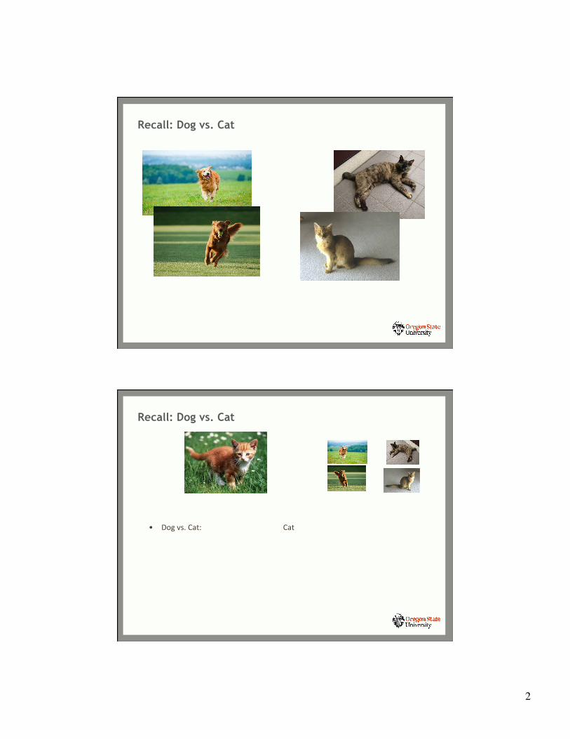
Recall: Dog vs. Cat
• Dog vs. Cat: Cat
Recall: Dog vs. Cat

3
Recall:
• Dog vs. Cat: Cat
• Movement vs. staYonary “Dog” maybe • Indoor vs. outdoor “Dog”
• Red vs. not red animal “Dog”
Recall: Dog vs. Cat or ???

4
Let’s revisit what happens in such a mapping
Label: “Motorcycle” Suggest tags Image search …
Speech recogniYon Music classificaYon Speaker idenYficaYon …
Web search AnY-‐spam Machine translaYon …
text
audio
images/video
Input: X Output: Y
ML
ML
ML
We want to map this picture to a label …
“motorcycle” ML
5
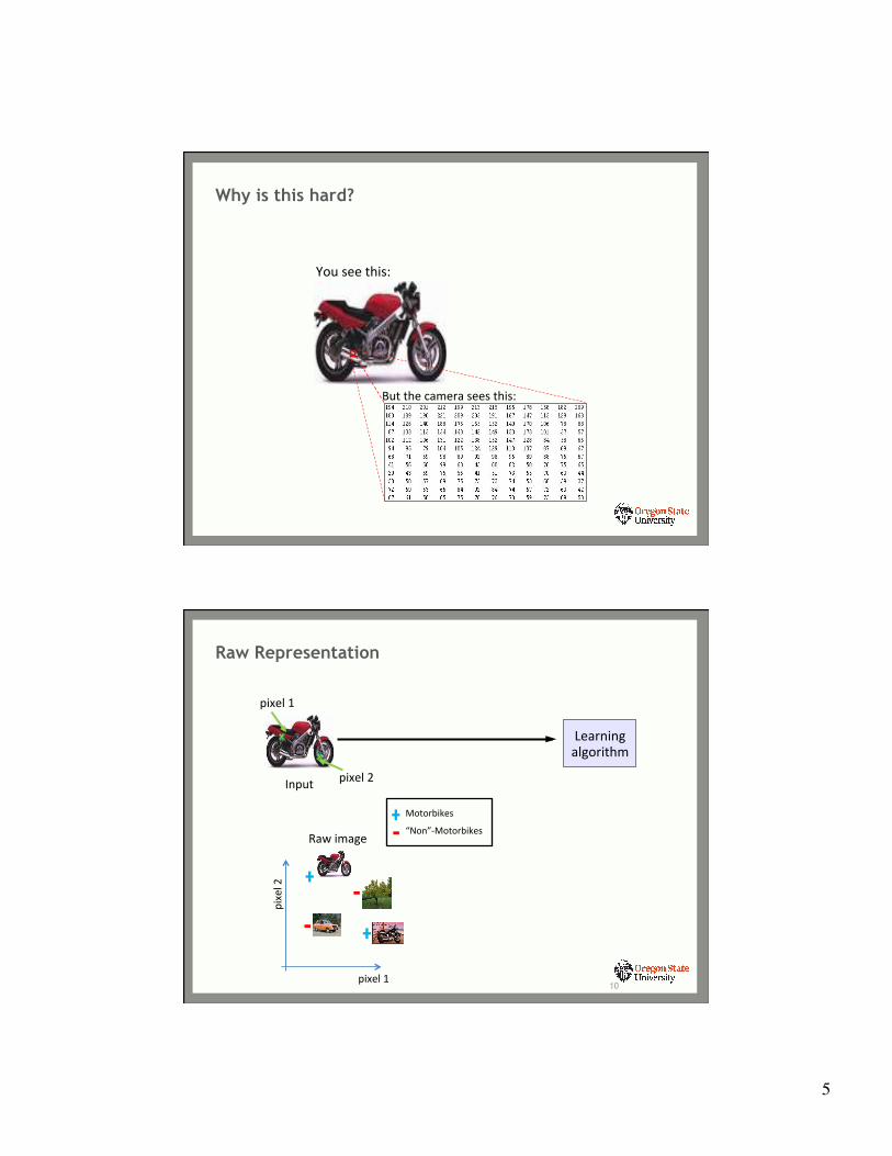
Why is this hard?
You see this:
But the camera sees this:
Raw Representation
Input
Raw image
Motorbikes
“Non”-‐Motorbikes
Learning algorithm
pixel 1
pixel 2
pixel 1
pixel 2
10
6
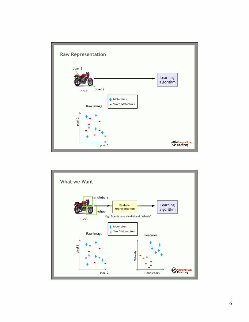
Raw Representation
Input
Motorbikes
“Non”-‐Motorbikes
Learning algorithm
pixel 1
pixel 2
pixel 1
pixel 2
Raw image
What we Want
Input
Motorbikes
“Non”-‐Motorbikes
Learning algorithm
pixel 1
pixel 2
Raw image
Handlebars
Whe
els
Features
handlebars
wheel
Feature representaYon
E.g., Does it have Handlebars? Wheels?
7
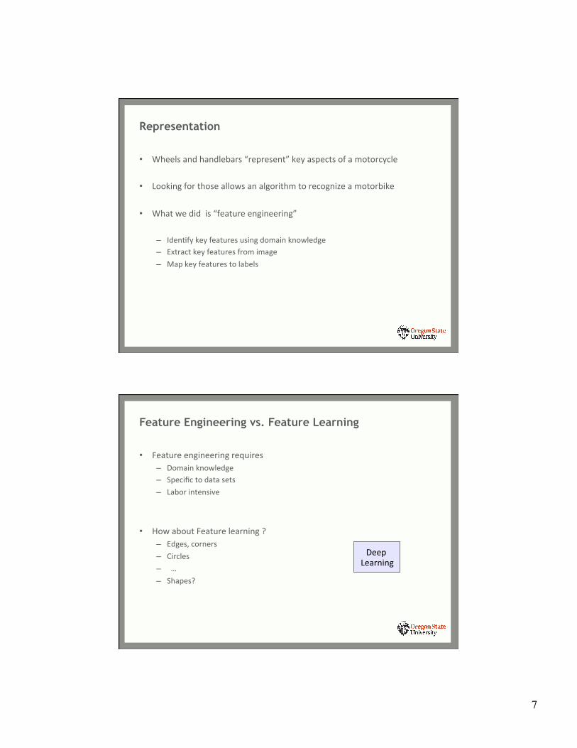
• Wheels and handlebars “represent” key aspects of a motorcycle
• Looking for those allows an algorithm to recognize a motorbike
• What we did is “feature engineering”
– IdenYfy key features using domain knowledge – Extract key features from image – Map key features to labels
Representation
• Feature engineering requires – Domain knowledge – Specific to data sets – Labor intensive
• How about Feature learning ? – Edges, corners – Circles – … – Shapes?
Feature Engineering vs. Feature Learning
Deep Learning

8
Deep Learning: Let’s learn the representation!
pixels edges object parts object models shapes
nose, eye Joe … happy corners
Deep Learning
Neural Network architecture with many layers
… wait a minute…
… is this new? Different than “just” neural networks?
Yes and No
9
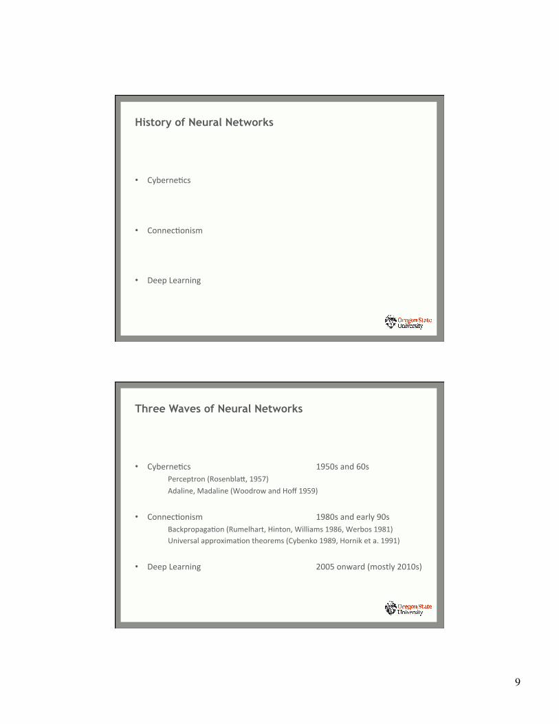
• CyberneYcs
• ConnecYonism
• Deep Learning
History of Neural Networks
• CyberneYcs 1950s and 60s Perceptron (Rosenblaf, 1957) Adaline, Madaline (Woodrow and Hoff 1959)
• ConnecYonism 1980s and early 90s BackpropagaYon (Rumelhart, Hinton, Williams 1986, Werbos 1981) Universal approximaYon theorems (Cybenko 1989, Hornik et a. 1991)
• Deep Learning 2005 onward (mostly 2010s)
Three Waves of Neural Networks

10
• CyberneYcs 1950s and 60s
1970s : Disillusionment 1 -‐ XOR (Minski, Papert 1969)
• ConnecYonism 1980s and early 90s ~1995-‐2005 : Disillusionment 2 -‐ (Support Vector Machine …)
• Deep Learning 2005 onward (mostly 2010s)
Three Waves of Neural Networks
First Two Waves Focused on
One hidden layer NNs Two hidden layer NNs
11
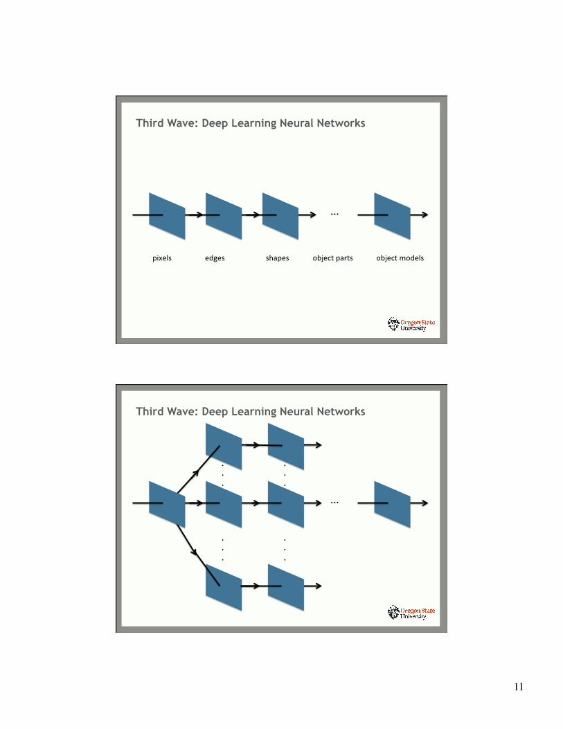
Third Wave: Deep Learning Neural Networks
…
pixels edges object parts object models shapes
Third Wave: Deep Learning Neural Networks
…
.
.
.
.
.
.
.
.
.
.
.
.
12
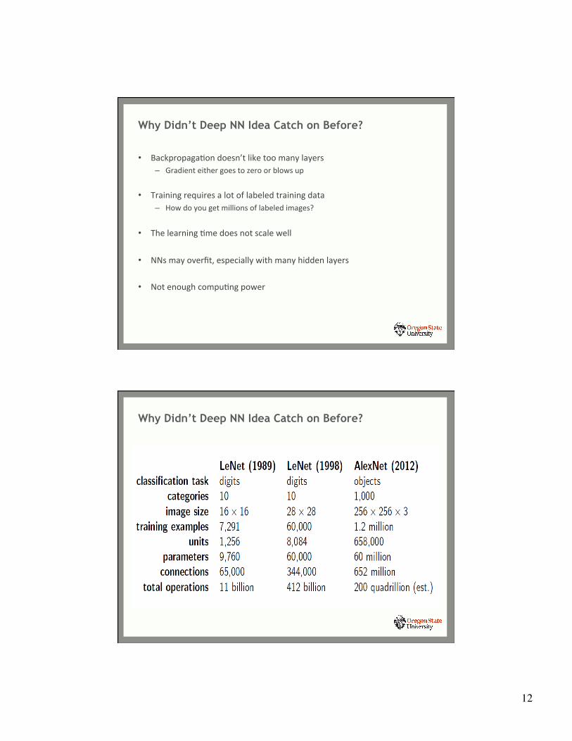
Why Didn’t Deep NN Idea Catch on Before?
• BackpropagaYon doesn’t like too many layers – Gradient either goes to zero or blows up
• Training requires a lot of labeled training data – How do you get millions of labeled images?
• The learning Yme does not scale well
• NNs may overfit, especially with many hidden layers
• Not enough compuYng power
Why Didn’t Deep NN Idea Catch on Before?
13
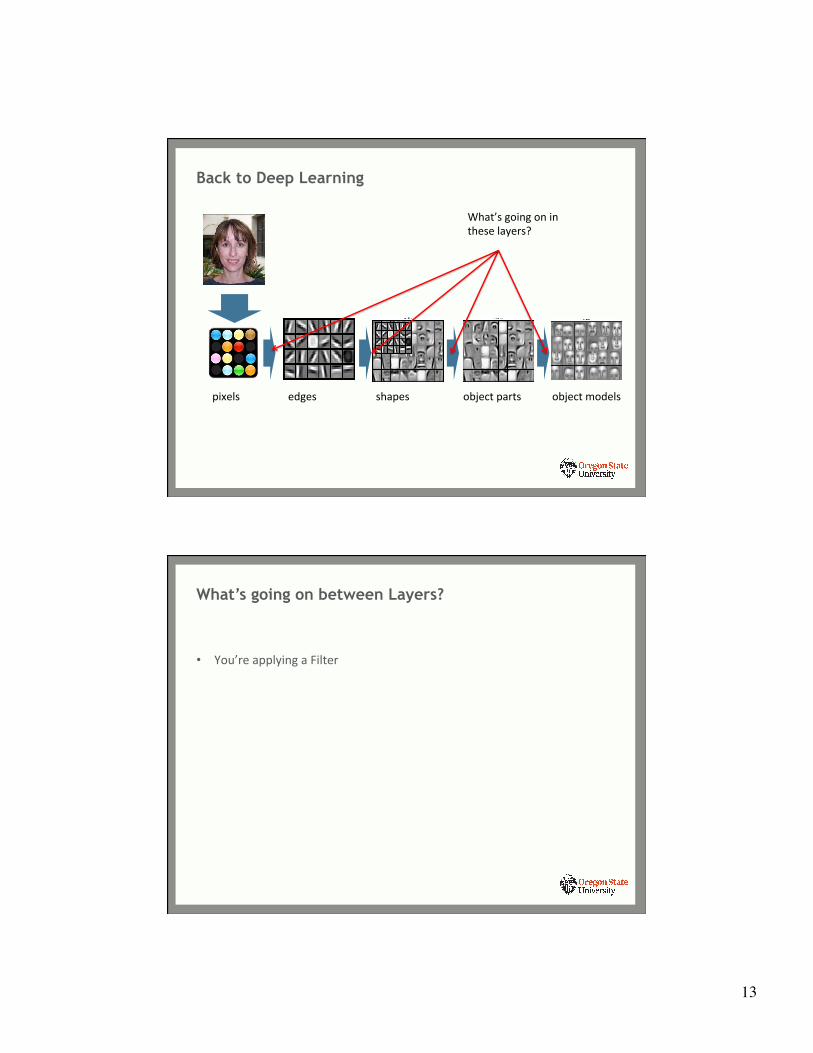
Back to Deep Learning
pixels edges object parts object models shapes
What’s going on in these layers?
• You’re applying a Filter
What’s going on between Layers?
14
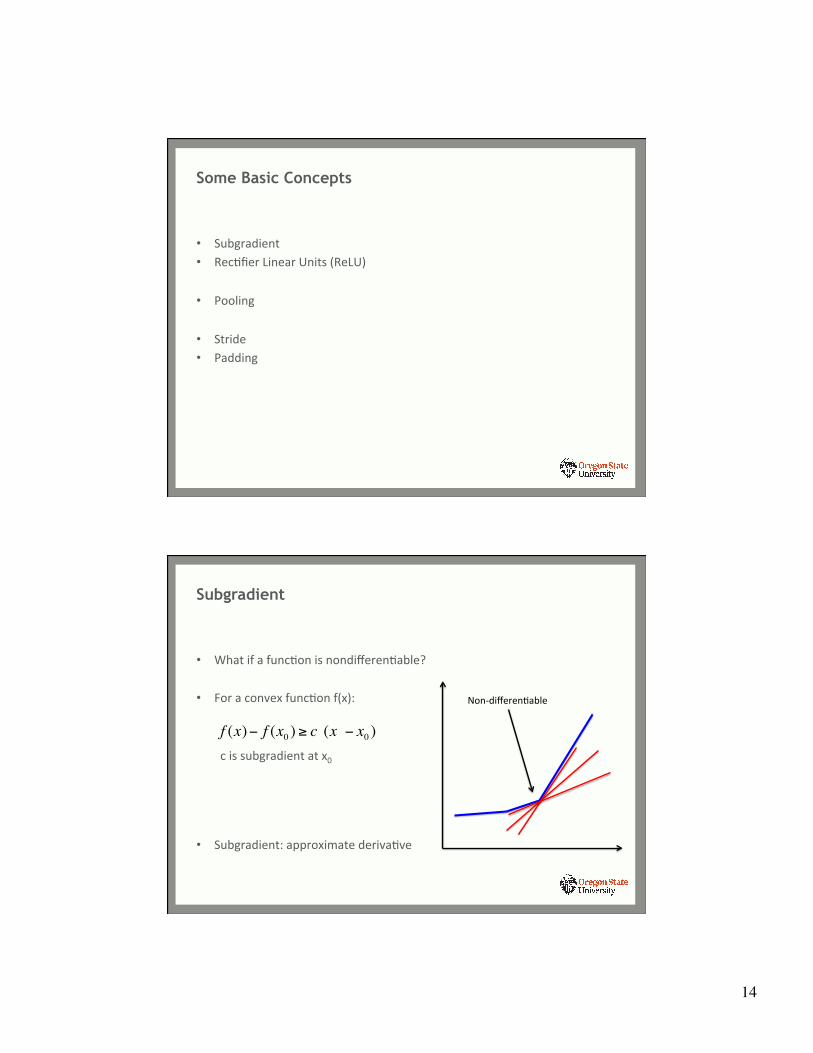
• Subgradient • RecYfier Linear Units (ReLU) • Pooling
• Stride • Padding
Some Basic Concepts
• What if a funcYon is nondifferenYable? • For a convex funcYon f(x):
c is subgradient at x0
• Subgradient: approximate derivaYve
Subgradient
Non-‐differenYable
f (x)− f (x0 ) ≥ c (x − x0 )
15
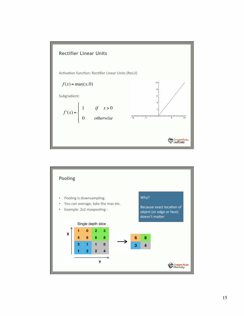
AcYvaYon funcYon: RecYfier Linear Units (ReLU)
Subgradient:
Rectifier Linear Units
f (x) =max(x, 0)
f '(x) =1 if x > 0
0 otherwise
!
"#
$#
• Pooling is downsampling. • You can average, take the max etc. • Example: 2x2 maxpooling :
Pooling
Why? Because exact locaYon of object (or edge or face) doesn’t mafer
16
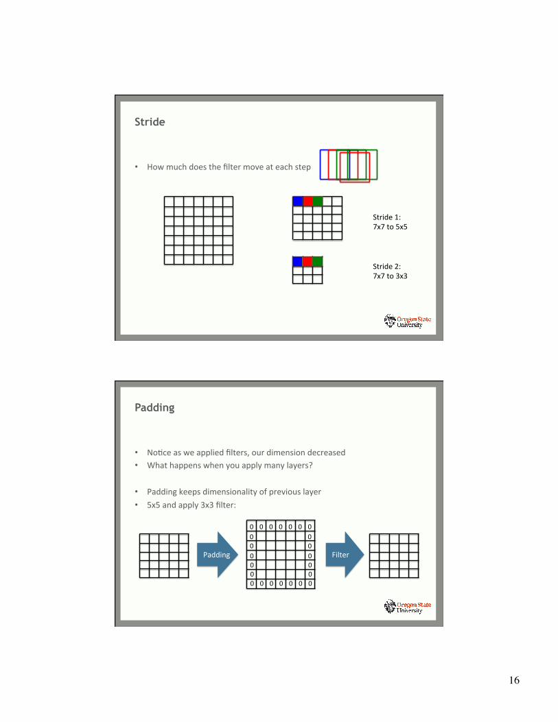
• How much does the filter move at each step
Stride
Stride 1: 7x7 to 5x5
Stride 2: 7x7 to 3x3
• NoYce as we applied filters, our dimension decreased • What happens when you apply many layers?
• Padding keeps dimensionality of previous layer • 5x5 and apply 3x3 filter:
Padding
0 0 0 0 0 0 0
0 0 0 0 0 0 0 0 0 0 0 0 0 0 0 0 0
Padding Filter
17
• Exploit structure in image
• Neighboring pixels carry local correlaYon
• Shapes carry long-‐range correlaYon
Convolutional Neural Networks
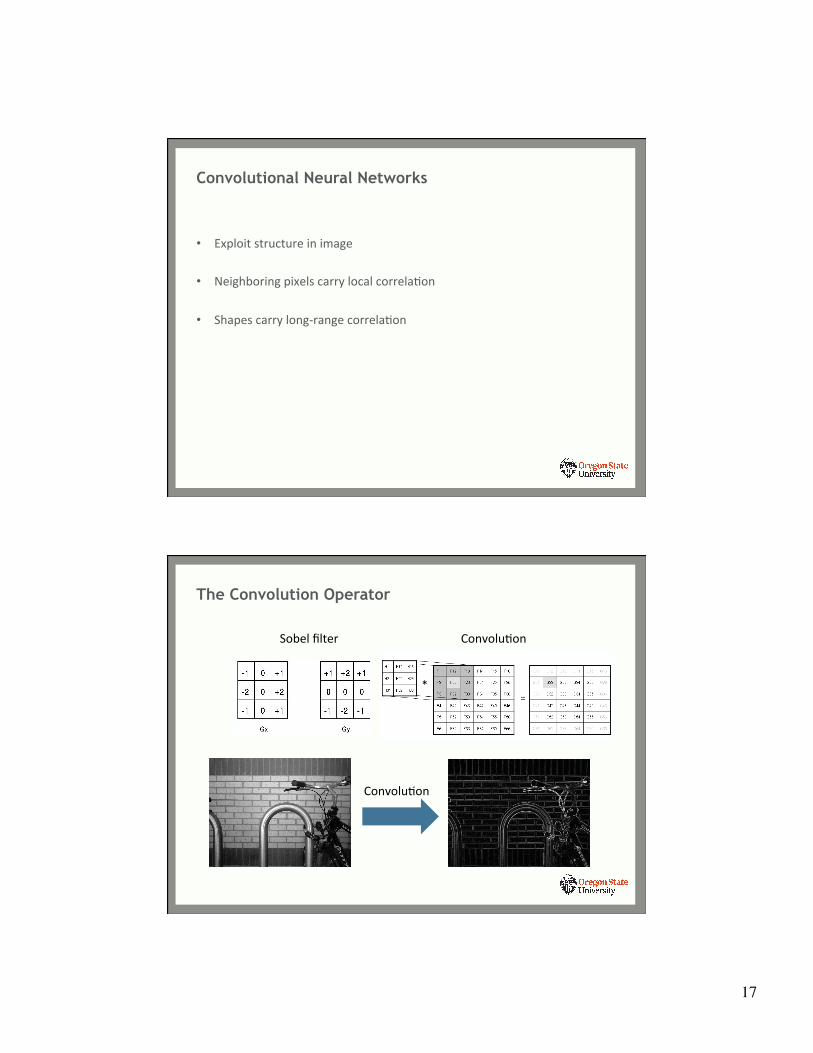
The Convolution Operator
ConvoluYon Sobel filter
ConvoluYon
*
18
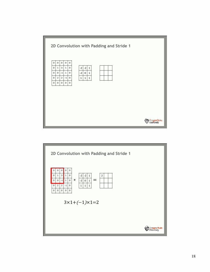
2D Convolution with Padding and Stride 1
0 0 0 0 0
0 1 3 1 0
0 0 -‐1 1 0
0 2 2 -‐1 0
0 0 0 0 0
-‐2 -‐2 1
-‐2 0 1
1 1 1
2D Convolution with Padding and Stride 1
0 0 0 0 0
0 1 3 1 0
0 0 -‐1 1 0
0 2 2 -‐1 0
0 0 0 0 0
∗-‐2 -‐2 1
-‐2 0 1
1 1 1
=2
3×1+(−1)×1=2
19
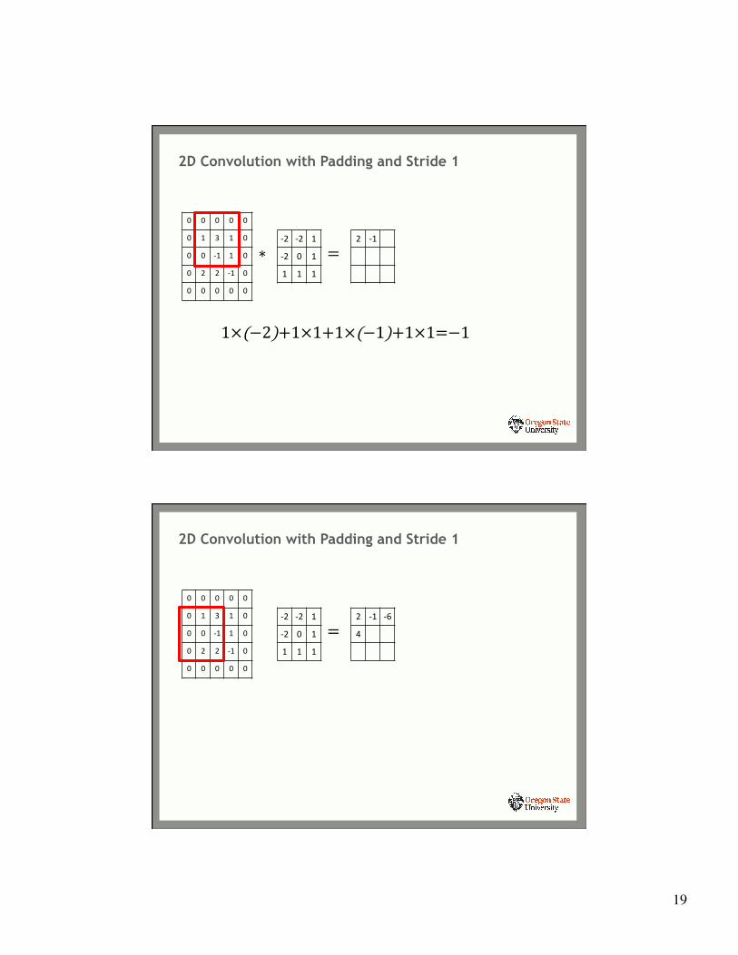
2D Convolution with Padding and Stride 1
0 0 0 0 0
0 1 3 1 0
0 0 -‐1 1 0
0 2 2 -‐1 0
0 0 0 0 0
∗-‐2 -‐2 1
-‐2 0 1
1 1 1
=2 -‐1
1×(−2)+1×1+1×(−1)+1×1=−1
2D Convolution with Padding and Stride 1
0 0 0 0 0
0 1 3 1 0
0 0 -‐1 1 0
0 2 2 -‐1 0
0 0 0 0 0
-‐2 -‐2 1
-‐2 0 1
1 1 1
=2 -‐1 -‐6
4

20
2D Convolution with Padding and Stride 1
0 0 0 0 0
0 1 3 1 0
0 0 -‐1 1 0
0 2 2 -‐1 0
0 0 0 0 0
∗-‐2 -‐2 1
-‐2 0 1
1 1 1
=2 -‐1 -‐6
4 -‐3
2D Convolution with Padding and Stride 1
0 0 0 0 0
0 1 3 1 0
0 0 -‐1 1 0
0 2 2 -‐1 0
0 0 0 0 0
∗-‐2 -‐2 1
-‐2 0 1
1 1 1
=2 -‐1 -‐6
4 -‐3 -‐5
21
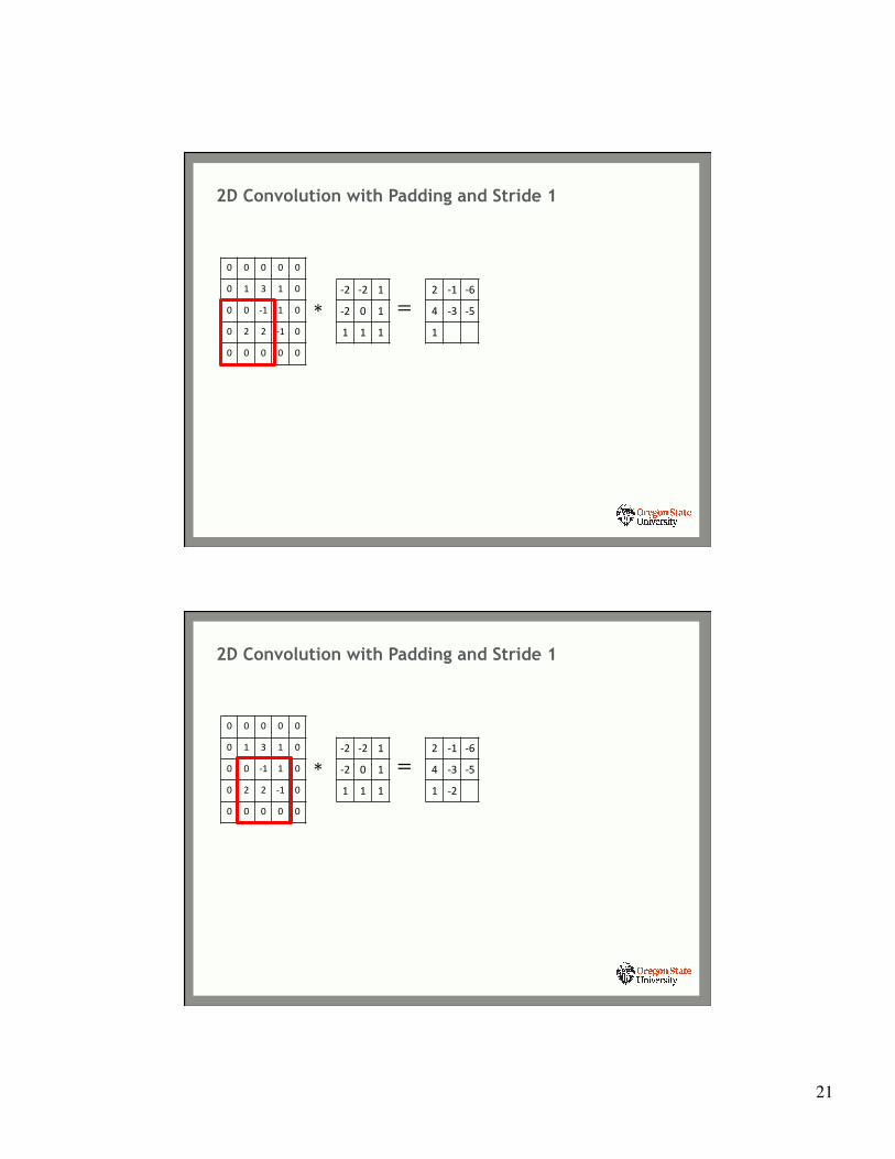
2D Convolution with Padding and Stride 1
0 0 0 0 0
0 1 3 1 0
0 0 -‐1 1 0
0 2 2 -‐1 0
0 0 0 0 0
∗-‐2 -‐2 1
-‐2 0 1
1 1 1
=2 -‐1 -‐6
4 -‐3 -‐5
1
2D Convolution with Padding and Stride 1
0 0 0 0 0
0 1 3 1 0
0 0 -‐1 1 0
0 2 2 -‐1 0
0 0 0 0 0
∗-‐2 -‐2 1
-‐2 0 1
1 1 1
=2 -‐1 -‐6
4 -‐3 -‐5
1 -‐2
22
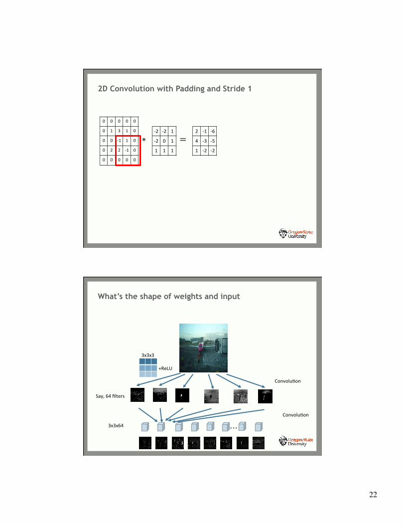
2D Convolution with Padding and Stride 1
0 0 0 0 0
0 1 3 1 0
0 0 -‐1 1 0
0 2 2 -‐1 0
0 0 0 0 0
∗-‐2 -‐2 1
-‐2 0 1
1 1 1
=2 -‐1 -‐6
4 -‐3 -‐5
1 -‐2 -‐2
What’s the shape of weights and input
…3x3x64
ConvoluYon
+ReLU
3x3x3
Say, 64 filters
ConvoluYon
23
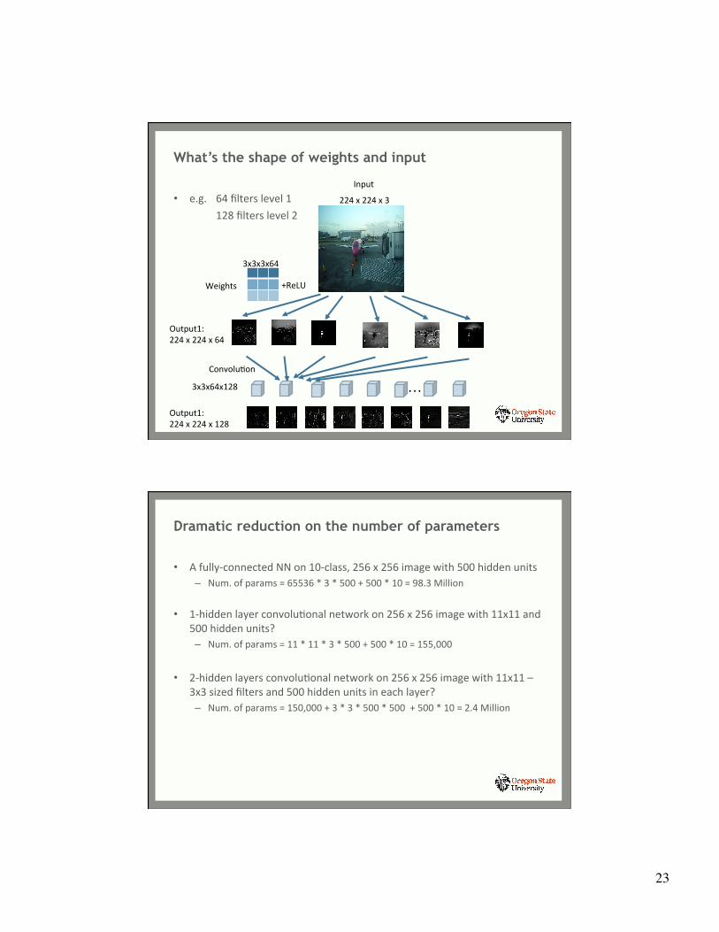
What’s the shape of weights and input
• e.g. 64 filters level 1 128 filters level 2
…3x3x64x128
ConvoluYon
+ReLU
3x3x3x64
224 x 224 x 3
Input
Weights
Output1: 224 x 224 x 64
Output1: 224 x 224 x 128
Dramatic reduction on the number of parameters
• A fully-‐connected NN on 10-‐class, 256 x 256 image with 500 hidden units – Num. of params = 65536 * 3 * 500 + 500 * 10 = 98.3 Million
• 1-‐hidden layer convoluYonal network on 256 x 256 image with 11x11 and 500 hidden units? – Num. of params = 11 * 11 * 3 * 500 + 500 * 10 = 155,000
• 2-‐hidden layers convoluYonal network on 256 x 256 image with 11x11 – 3x3 sized filters and 500 hidden units in each layer? – Num. of params = 150,000 + 3 * 3 * 500 * 500 + 500 * 10 = 2.4 Million
24
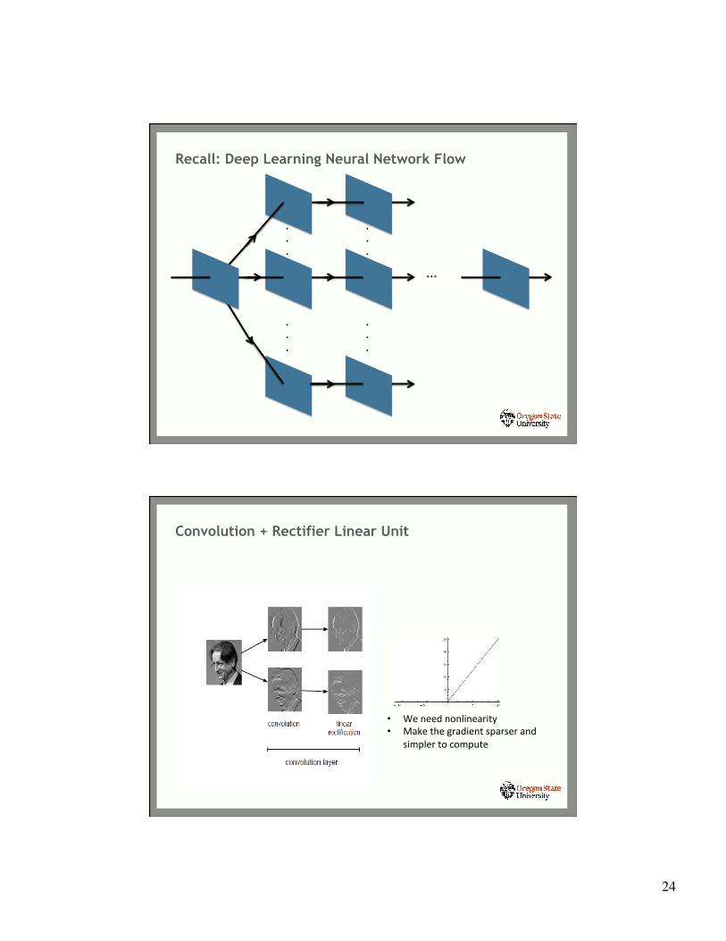
Recall: Deep Learning Neural Network Flow
…
.
.
.
.
.
.
.
.
.
.
.
.
Convolution + Rectifier Linear Unit
• We need nonlinearity • Make the gradient sparser and
simpler to compute
25
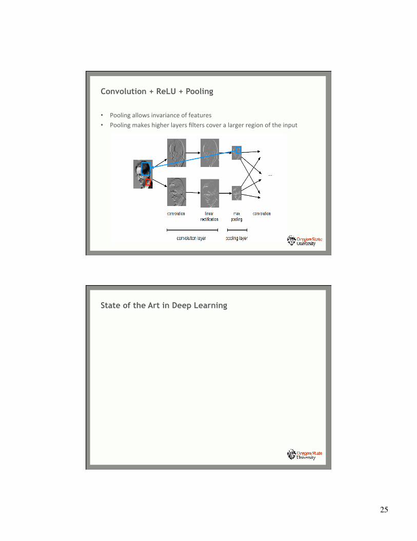
Convolution + ReLU + Pooling
• Pooling allows invariance of features • Pooling makes higher layers filters cover a larger region of the input
State of the Art in Deep Learning
26
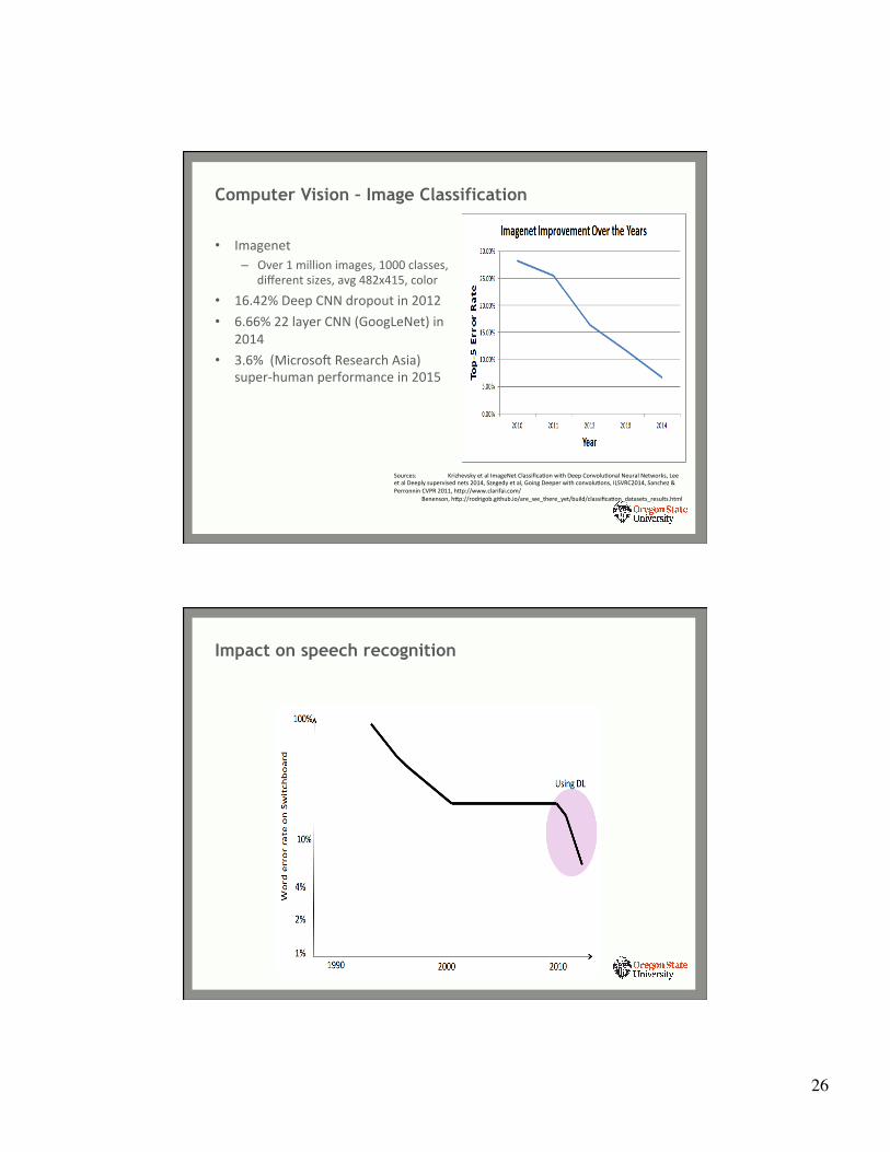
Computer Vision – Image Classification
• Imagenet – Over 1 million images, 1000 classes,
different sizes, avg 482x415, color
• 16.42% Deep CNN dropout in 2012 • 6.66% 22 layer CNN (GoogLeNet) in
2014 • 3.6% (Microsot Research Asia)
super-‐human performance in 2015
Sources: Krizhevsky et al ImageNet ClassificaYon with Deep ConvoluYonal Neural Networks, Lee et al Deeply supervised nets 2014, Szegedy et al, Going Deeper with convoluYons, ILSVRC2014, Sanchez & Perronnin CVPR 2011, hfp://www.clarifai.com/
Benenson, hfp://rodrigob.github.io/are_we_there_yet/build/classificaYon_datasets_results.html
Impact on speech recognition
27
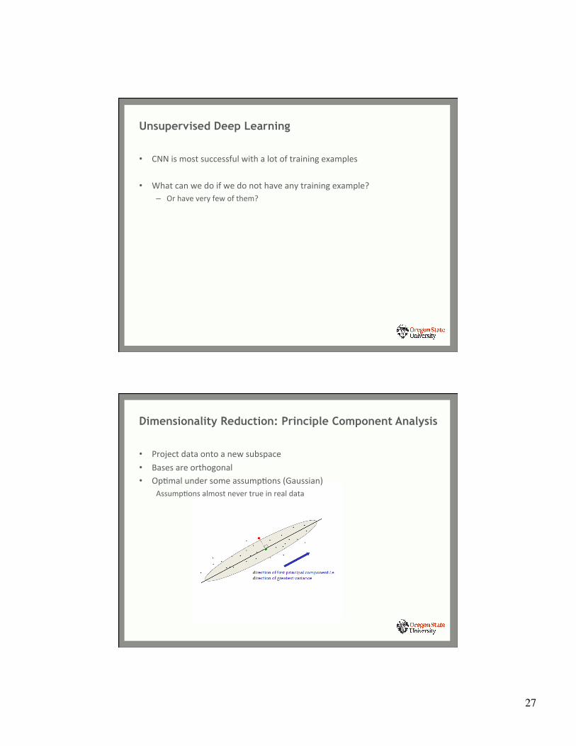
Unsupervised Deep Learning
• CNN is most successful with a lot of training examples
• What can we do if we do not have any training example? – Or have very few of them?
Dimensionality Reduction: Principle Component Analysis
• Project data onto a new subspace • Bases are orthogonal • OpYmal under some assumpYons (Gaussian)
AssumpYons almost never true in real data
28
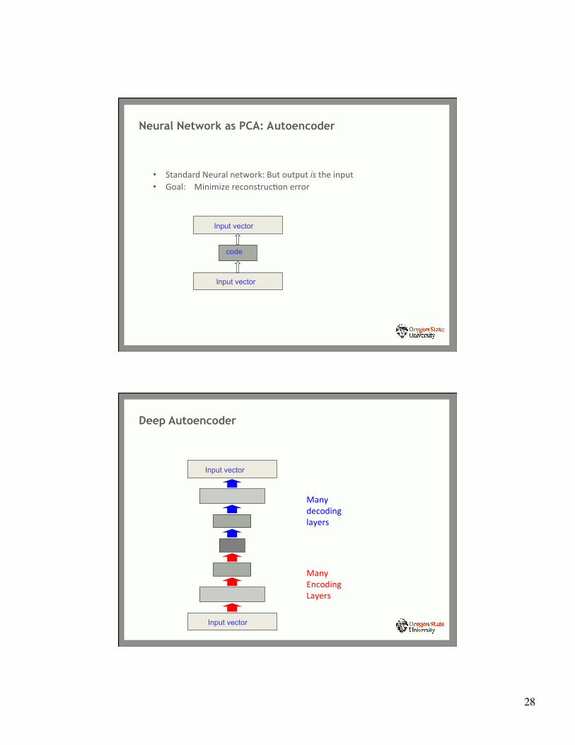
Input vector
Input vector
code
• Standard Neural network: But output is the input • Goal: Minimize reconstrucYon error
Neural Network as PCA: A utoencoder
Input vector
Input vector
Deep Autoencoder
Many Encoding Layers
Many decoding layers
29
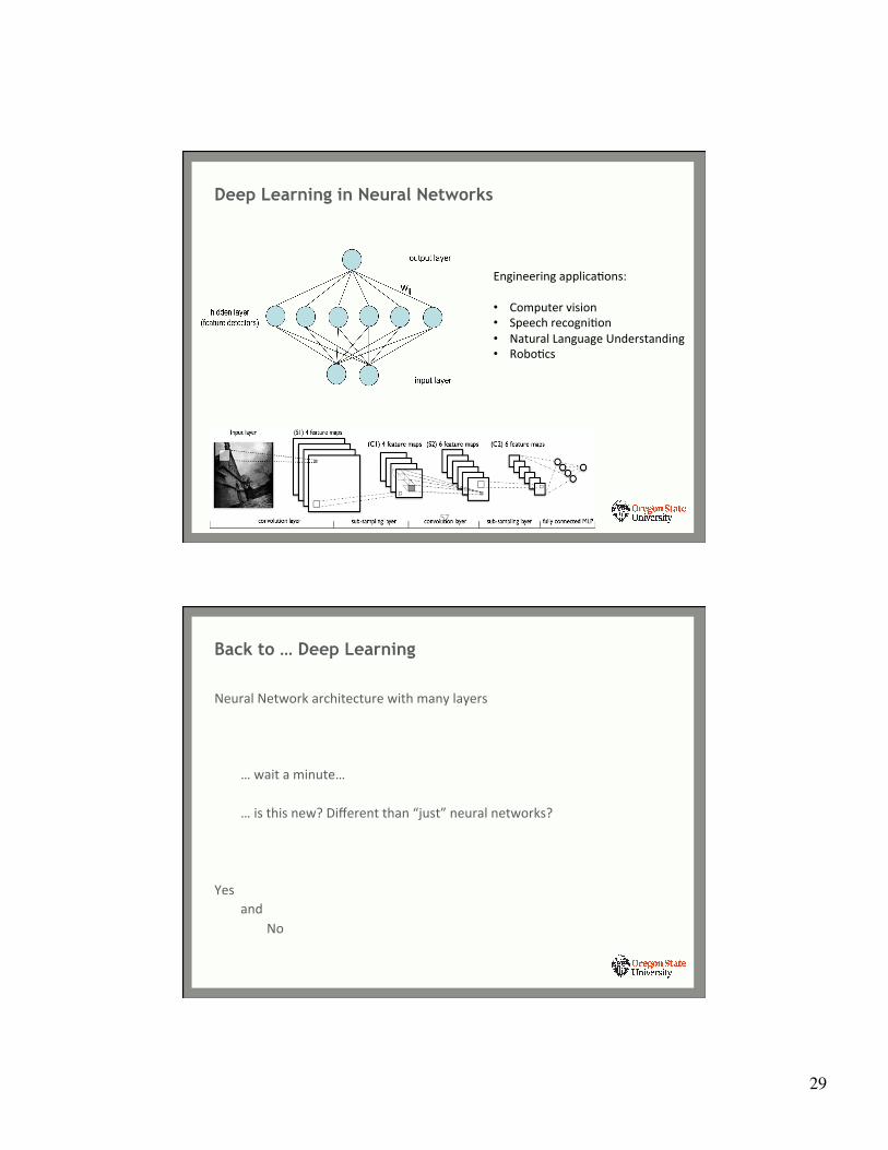
Engineering applicaYons: • Computer vision • Speech recogniYon • Natural Language Understanding • RoboYcs
57
Deep Learning in Neural Networks
Back to … Deep Learning
Neural Network architecture with many layers
… wait a minute…
… is this new? Different than “just” neural networks? Yes
and No

30
Why Didn’t Deep NN Idea Catch on Before?
• Not clear what deep fully connected networks learn
• BackpropagaYon doesn’t like too many layers – Gradient either goes to zero or blows up
• Training requires a lot of labeled training data – Million+ labeled images (Amazon Mechanical Turk)
• The learning Yme does not scale well
• NNs tend to overfit, especially with many hidden layers
• Not enough compuYng power
So What’s New ?
• ConvoluYon neural networks
• New acYvaYon funcYons and subgradients – ReLU
• Everything is on the internet … A lot of labeled data – Million+ labeled images (Amazon Mechanical Turk)
• More efficient learning algorithms: stochasYc gradient descent
• Pooling (dimensionality control)
• Much befer compuYng power … GPUs
31
What’s Next ?
Deep Learning: Methods and ApplicaYons, L. Deng and D. Yu, “FoundaYons and Trends in Signal Processing,” Vol. 7, Nos. 3–4, 197–387, 2013. (also, hfp://en.wikipedia.org/wiki/Hype_cycle )
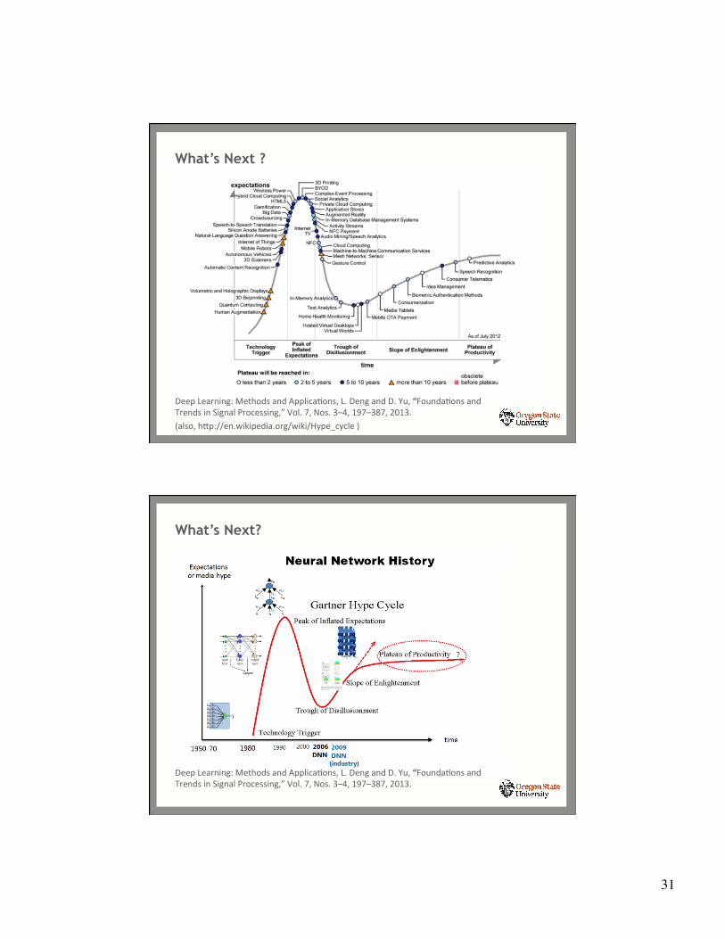
What’s Next?
Deep Learning: Methods and ApplicaYons, L. Deng and D. Yu, “FoundaYons and Trends in Signal Processing,” Vol. 7, Nos. 3–4, 197–387, 2013.