robin genuer jean-michel poggi random forests with r
TRANSCRIPT

Use R !
Robin GenuerJean-Michel Poggi
Random Forests with R

Use R!
Series Editors
Robert Gentleman, 23andMe Inc., South San Francisco, USA
Kurt Hornik, Department of Finance, Accounting and Statistics, WUWirtschaftsuniversität Wien, Vienna, Austria
Giovanni Parmigiani, Dana-Farber Cancer Institute, Boston, USA

This series of inexpensive and focused books on R will publish shorter booksaimed at practitioners. Books can discuss the use of R in a particular subject area(e.g., epidemiology, econometrics, psychometrics) or as it relates to statistical topics(e.g., missing data, longitudinal data). In most cases, books will combine LaTeXand R so that the code for figures and tables can be put on a website. Authorsshould assume a background as supplied by Dalgaard’s Introductory Statistics withR or other introductory books so that each book does not repeat basic material.
More information about this series at http://www.springer.com/series/6991
Use R!

Robin Genuer • Jean-Michel Poggi
Random Forests with R
123

Robin GenuerISPEDUniversity of BordeauxBordeaux, France
Jean-Michel PoggiLab. Maths Orsay (LMO)Paris-Saclay UniversityOrsay, France
ISSN 2197-5736 ISSN 2197-5744 (electronic)Use R!ISBN 978-3-030-56484-1 ISBN 978-3-030-56485-8 (eBook)https://doi.org/10.1007/978-3-030-56485-8
Translation from the French language edition: Les forêts aléatoires avec R by Robin Genuer andJean-Michel Poggi © Presses Universitaires de Rennes 2019 All Rights Reserved© Springer Nature Switzerland AG 2020This work is subject to copyright. All rights are reserved by the Publisher, whether the whole or partof the material is concerned, specifically the rights of translation, reprinting, reuse of illustrations,recitation, broadcasting, reproduction on microfilms or in any other physical way, and transmissionor information storage and retrieval, electronic adaptation, computer software, or by similar or dissimilarmethodology now known or hereafter developed.The use of general descriptive names, registered names, trademarks, service marks, etc. in thispublication does not imply, even in the absence of a specific statement, that such names are exempt fromthe relevant protective laws and regulations and therefore free for general use.The publisher, the authors and the editors are safe to assume that the advice and information in thisbook are believed to be true and accurate at the date of publication. Neither the publisher nor theauthors or the editors give a warranty, expressed or implied, with respect to the material containedherein or for any errors or omissions that may have been made. The publisher remains neutral with regardto jurisdictional claims in published maps and institutional affiliations.
This Springer imprint is published by the registered company Springer Nature Switzerland AGThe registered company address is: Gewerbestrasse 11, 6330 Cham, Switzerland

Preface
Random forests are a statistical learning method introduced by Leo Breiman in 2001.They are extensively used in many fields of application, due for sure not only to theirexcellent predictive performance, but also to their flexibility, with a few restrictionson the nature of the data. Indeed, random forests are adapted to both supervisedclassification problems and regression problems. In addition, they allow to considerqualitative and quantitative explanatory variables together without preprocessing.Moreover, they can be used to process standard data for which the number ofobservations is higher than the number of variables, while also performing very wellin the high dimensional case, where the number of variables is quite large in com-parison to the number of observations. Consequently, they are now among preferredmethods in the toolbox of statisticians and other data scientists.
Who Is This Book for?
This book is an application-oriented statistical presentation of random forests. It istherefore primarily intended not only for students in academic fields such as statisticaleducation, but also for practitioners in statistics and machine learning. A scientificundergraduate degree is quite sufficient to take full advantage of the concepts, methods,and tools covered by the book. In terms of computer science skills, little backgroundknowledge is required, though an introduction to the R language is recommended.
Book Content
Random forests are part of the family of tree-based methods; accordingly, after anintroductory chapter, Chap. 2 presents CART trees. The next three chapters aredevoted to random forests. They focus on their presentation (Chap. 3), on the
v

variable importance tool (Chap. 4), and on the variable selection problem (Chap. 5),respectively.
The structure of the chapters (except the introduction) is always the same. After apresentation of the concepts and methods, we illustrate their implementation on arunning example. Then, various complements are provided before examiningadditional examples.
Throughout the book, each result is given together with the R code that can beused to reproduce it. All lines of code are available online1 making things easy.
Thus, the book offers readers essential information and concepts, together withexamples and the software tools needed to analyze data using random forests.
Orsay, France Robin GenuerJune 2020 Jean-Michel Poggi
1https://RFwithR.robin.genuer.fr.
vi Preface

Acknowledgements
Our first thanks go to Eva Hiripi who suggested the idea of publishing the Englishversion of the French original edition of the book entitled “Les forêts aléatoires avecR” (Presses Universitaires de Rennes Ed.).
We would like to thank our colleagues who shared our thoughts about thesetopics through numerous collaborations, in particular, Sylvain Arlot, Servane Gey,Christine Tuleau-Malot, and Nathalie Villa-Vialaneix.
We would also like to thank Nicolas Bousquet and Fabien Navarro who saved usa lot of time by providing us a first raw translation, thanks to the tool theydeveloped for a large-scale automatic translation conducted in 2018. Of course, theauthors are entirely responsible for the final translated version.
Finally, we thank three anonymous reviewers for their useful comments andinsightful suggestions.
vii

Contents
1 Introduction to Random Forests with R . . . . . . . . . . . . . . . . . . . . . . 11.1 Preamble . . . . . . . . . . . . . . . . . . . . . . . . . . . . . . . . . . . . . . . . . . 11.2 Notation . . . . . . . . . . . . . . . . . . . . . . . . . . . . . . . . . . . . . . . . . . . 21.3 Statistical Objectives . . . . . . . . . . . . . . . . . . . . . . . . . . . . . . . . . . 31.4 Packages . . . . . . . . . . . . . . . . . . . . . . . . . . . . . . . . . . . . . . . . . . 41.5 Datasets . . . . . . . . . . . . . . . . . . . . . . . . . . . . . . . . . . . . . . . . . . . 5
1.5.1 Running Example: Spam Detection . . . . . . . . . . . . . . . . . . 51.5.2 Ozone Pollution . . . . . . . . . . . . . . . . . . . . . . . . . . . . . . . . 61.5.3 Genomic Data for a Vaccine Study . . . . . . . . . . . . . . . . . . 71.5.4 Dust Pollution . . . . . . . . . . . . . . . . . . . . . . . . . . . . . . . . . 7
2 CART . . . . . . . . . . . . . . . . . . . . . . . . . . . . . . . . . . . . . . . . . . . . . . . . 92.1 The Principle . . . . . . . . . . . . . . . . . . . . . . . . . . . . . . . . . . . . . . . 92.2 Maximal Tree Construction . . . . . . . . . . . . . . . . . . . . . . . . . . . . . 102.3 Pruning . . . . . . . . . . . . . . . . . . . . . . . . . . . . . . . . . . . . . . . . . . . 132.4 The rpart Package . . . . . . . . . . . . . . . . . . . . . . . . . . . . . . . . . . . 162.5 Competing and Surrogate Splits . . . . . . . . . . . . . . . . . . . . . . . . . 22
2.5.1 Competing Splits . . . . . . . . . . . . . . . . . . . . . . . . . . . . . . . 222.5.2 Surrogate Splits . . . . . . . . . . . . . . . . . . . . . . . . . . . . . . . . 232.5.3 Interpretability . . . . . . . . . . . . . . . . . . . . . . . . . . . . . . . . . 24
2.6 Examples . . . . . . . . . . . . . . . . . . . . . . . . . . . . . . . . . . . . . . . . . . 262.6.1 Predicting Ozone Concentration . . . . . . . . . . . . . . . . . . . . 262.6.2 Analyzing Genomic Data . . . . . . . . . . . . . . . . . . . . . . . . . 29
3 Random Forests . . . . . . . . . . . . . . . . . . . . . . . . . . . . . . . . . . . . . . . . 333.1 General Principle . . . . . . . . . . . . . . . . . . . . . . . . . . . . . . . . . . . . 33
3.1.1 Instability of a Tree . . . . . . . . . . . . . . . . . . . . . . . . . . . . . 343.1.2 From a Tree to an Ensemble: Bagging . . . . . . . . . . . . . . . 37
3.2 Random Forest Random Inputs . . . . . . . . . . . . . . . . . . . . . . . . . . 393.3 The randomForest Package . . . . . . . . . . . . . . . . . . . . . . . . . . . . 41
ix

3.4 Out-Of-Bag Error . . . . . . . . . . . . . . . . . . . . . . . . . . . . . . . . . . . . 423.5 Parameters Setting for Prediction . . . . . . . . . . . . . . . . . . . . . . . . . 43
3.5.1 The Number of Trees: ntree . . . . . . . . . . . . . . . . . . . . . 433.5.2 The Number of Variables Chosen at Each
Node: mtry . . . . . . . . . . . . . . . . . . . . . . . . . . . . . . . . . . 443.6 Examples . . . . . . . . . . . . . . . . . . . . . . . . . . . . . . . . . . . . . . . . . . 47
3.6.1 Predicting Ozone Concentration . . . . . . . . . . . . . . . . . . . . 473.6.2 Analyzing Genomic Data . . . . . . . . . . . . . . . . . . . . . . . . . 503.6.3 Analyzing Dust Pollution . . . . . . . . . . . . . . . . . . . . . . . . . 52
4 Variable Importance . . . . . . . . . . . . . . . . . . . . . . . . . . . . . . . . . . . . . 574.1 Notions of Importance . . . . . . . . . . . . . . . . . . . . . . . . . . . . . . . . 574.2 Variable Importance Behavior . . . . . . . . . . . . . . . . . . . . . . . . . . . 61
4.2.1 Behavior According to n and p . . . . . . . . . . . . . . . . . . . . . 614.2.2 Behavior for Groups of Correlated Variables . . . . . . . . . . . 63
4.3 Tree Diversity and Variables Importance . . . . . . . . . . . . . . . . . . . 654.4 Influence of Parameters on Variable Importance . . . . . . . . . . . . . . 664.5 Examples . . . . . . . . . . . . . . . . . . . . . . . . . . . . . . . . . . . . . . . . . . 68
4.5.1 An Illustration by Simulation in Regression . . . . . . . . . . . 684.5.2 Predicting Ozone Concentration . . . . . . . . . . . . . . . . . . . . 694.5.3 Analyzing Genomic Data . . . . . . . . . . . . . . . . . . . . . . . . . 714.5.4 Air Pollution by Dust: What Is the Local
Contribution? . . . . . . . . . . . . . . . . . . . . . . . . . . . . . . . . . 74
5 Variable Selection . . . . . . . . . . . . . . . . . . . . . . . . . . . . . . . . . . . . . . . 775.1 Generalities . . . . . . . . . . . . . . . . . . . . . . . . . . . . . . . . . . . . . . . . 775.2 Principle . . . . . . . . . . . . . . . . . . . . . . . . . . . . . . . . . . . . . . . . . . 795.3 Procedure . . . . . . . . . . . . . . . . . . . . . . . . . . . . . . . . . . . . . . . . . . 795.4 The VSURF Package . . . . . . . . . . . . . . . . . . . . . . . . . . . . . . . . . 815.5 Parameter Setting for Selection . . . . . . . . . . . . . . . . . . . . . . . . . . 875.6 Examples . . . . . . . . . . . . . . . . . . . . . . . . . . . . . . . . . . . . . . . . . . 88
5.6.1 Predicting Ozone Concentration . . . . . . . . . . . . . . . . . . . . 885.6.2 Analyzing Genomic Data . . . . . . . . . . . . . . . . . . . . . . . . . 90
References . . . . . . . . . . . . . . . . . . . . . . . . . . . . . . . . . . . . . . . . . . . . . . . . . . 93
Index . . . . . . . . . . . . . . . . . . . . . . . . . . . . . . . . . . . . . . . . . . . . . . . . . . . . . . 97
x Contents

Chapter 1Introduction to Random Forests with R
Abstract The two algorithms discussed in this bookwere proposed byLeoBreiman:CART trees, which were introduced in the mid-1980s, and random forests, whichemerged just under 20 years later in the early 2000s. This chapter offers an intro-duction to the subject matter, beginning with a historical overview. Some notations,used to define the various statistical objectives addressed in the book, are also intro-duced: classification, regression, prediction, and variable selection. In turn, the threeR packages used in the book are listed, and some competitors are mentioned. Lastly,the four datasets used to illustrate themethods’ application are presented: the runningexample (spam), a genomic dataset, and two pollution datasets (ozone and dust).
1.1 Preamble
The two algorithms discussed in this book were proposed by Leo Breiman: CART(Classification AndRegression Trees) trees, whichwere introduced in themid-1980s(Breiman et al. 1984), and random forests (Breiman 2001), which emerged justunder 20 years later in the early 2000s. At the confluence of statistics and statisticallearning, this shortcut among Leo Breiman’s multiple contributions, whose scientificbiography is described in Olshen (2001) and Cutler (2010), provides a remarkablefigure of these two disciplines.
Decision trees are the basic tool for numerous tree-based ensemble methods.Although known for decades and very attractive because of their simplicity andinterpretability, their use suffered, until the 1980s, from serious justified objections.From this point of view, CART offers to decision trees the conceptual framework ofautomaticmodel selection, giving them theoretical guarantees andbroad applicabilitywhile preserving their ease of interpretation.
But one of themajor drawbacks, instability, remains. The idea of random forests isto exploit the natural variability of trees. More specifically, it is a matter of disruptingthe construction by introducing some randomness in the selection of both individualsand variables. The resulting trees are then combined to construct the final prediction,
© Springer Nature Switzerland AG 2020R. Genuer and J.-M. Poggi, Random Forests with R, Use R!,https://doi.org/10.1007/978-3-030-56485-8_1
1

2 1 Introduction to Random Forests with R
rather than choosing one of them. Several algorithms based on such principles havethus been developed, for many of them, by Breiman himself: Bagging (Breiman1996), several variants of the Arcing (Breiman 1998), and Adaboost (Freund andSchapire 1997).
Random forests (RF in the following) are therefore a nonparametric method ofstatistical learning widely used in many fields of application, such as the study ofmicroarrays (Díaz-Uriarte and Alvarez De Andres 2006), ecology (Prasad et al.2006), pollution prediction (Ghattas 1999), and genomics (Goldstein et al. 2010;Boulesteix et al. 2012), and for a broader review, see Verikas et al. (2011). Thisuniversality is first and foremost linked to excellent predictive performance. Thiscan be seen in Fernández-Delgado et al. (2014) which crowns RF in a recent large-scale comparative evaluation, whereas less than a decade earlier, the article in Wuet al. (2008) with similar objectives mentions CART but not yet random forests! Inaddition, they are applicable to many types of data. Indeed, it is possible to considerhigh-dimensional data for which the number of variables far exceeds the number ofobservations. In addition, they are suitable for both classification problems (categori-cal response variable) and regression problems (continuous response variable). Theyalso allow handling a mixture of qualitative and quantitative explanatory variables.Finally, they are, of course, able to process standard data for which the number ofobservations is greater than the number of variables.
Beyond the performance and the easy to tune feature of the method with veryfew parameters to adjust, one of the most important aspects in terms of applicationis the quantification of the explanatory variables’ relative importance. This concept,which is not so much examined by statisticians (see, for example, Grömping 2015, inregression), finds a convenient definition in the context of random forests that is easyto evaluate and which naturally extends to the case of groups of variables (Gregoruttiet al. 2015).
Therefore, and we will emphasize this aspect very strongly, RF can be used forvariable selection. Thus, in addition to a powerful prediction tool, it can also be usedto select the most interesting explanatory variables to explain the response, among apotentially very large number of variables. This is very attractive in practice becauseit helps both to interpretmore easily the results and, above all, to determine influentialfactors for the problem of interest. Finally, it can also be beneficial for prediction,because eliminating many irrelevant variables makes the learning task easier.
1.2 Notation
Throughout the book, we will adopt the following notations. We assume that a learn-ing sample is available:
Ln = {(X1,Y1), . . . , (Xn,Yn)}

1.2 Notation 3
composed of n couples of independent and identically distributed observations, com-ing from the same common distribution as a couple (X,Y ). This distribution is, ofcourse, unknown in practice and the purpose is precisely to estimate it, or morespecifically to estimate the link that exists between X and Y .
We call the coordinates of X the “input variables” (or “explanatory variables” or“variables”), where we note X j for the j th coordinate, and we assume that X ∈ X ,a certain space that we will specify later. However, we assume that this space is ofdimension p, where p is the (total) number of variables.
Y refers to the “response variable” (or “explained variable” or “dependent vari-able”) and Y ∈ Y . The nature of the regression or classification problem depends onthe nature of the space Y:
• If Y = R, we have a regression problem.• If Y = {1, . . . ,C}, we have a classification problem with C classes.
1.3 Statistical Objectives
PredictionThe first learning objective is prediction. We are trying, using the learning sampleLn , to construct a predictor:
h : X → Y
which associates a prediction y of the response variable corresponding to any giveninput observation x ∈ X .
The “hat” onh is a notation to specify that this predictor is constructed using Ln .We omit the dependence over n for the predictor to simplify the notations, but it doesexist.
More precisely, we want to build a powerful predictor in terms of prediction error(also called generalization error):
• In regression, we will consider here the mathematical expectation of the quadraticerror: E
[
(Y −h(X))2]
.• In classification, the probability of misclassification: P
(
Y �= h(X))
.
The prediction error depends on the unknown joint distribution of the randomcouple (X,Y ), so it must be estimated. One classical way to proceed is, using a testsample Tm = {(X ′
1, Y′1), . . . , (X
′m,Y
′m)}, also drawn from the distribution of (X,Y ),
to calculate an empirical test error:
• In regression, it is the mean square error: 1m
∑mi=1
(
Y ′i −h(X ′
i ))2.
• In classification, the misclassification rate: 1m
∑mi=1 1Y ′
i �=h(X ′i ).

4 1 Introduction to Random Forests with R
In the case where a test sample is not available, the prediction error can still beestimated, for example, by cross-validation. In addition, we will introduce later on aspecific estimate using random forests.
Remark 1.1 In this book, we focus on regression problems and/or supervised clas-sification ones. However, RF have been generalized to various other statistical prob-lems.
First, for survival data analysis, Ishwaran et al. (2008) introduced Random Sur-vival Forests, transposing the main ideas of RF to the case for which the quantityto be predicted is the time to event. Let us also mention on this subject the work ofHothorn et al. (2006).
Random forests have also been generalized to the multivariate response variablecase (see the review by Segal and Xiao 2011, which also provides references fromthe 1990s).
Selection and importance of variablesA second classical objective is variable selection. This involves determining a subsetof the input variables that are actually useful and active in explaining the input–outputrelationship. The quality of a subset of selected variables is often assessed by theperformance obtained with a predictor using only these variables instead of all theinitial sets.
In addition, we can focus on constructing a hierarchy of input variables based ona quantification of the importance of the effects on the output variable. Such an indexof importance therefore provides a ranking of variables, from the most important tothe least important.
1.4 Packages
We will mainly focus on R three packages (R Core Team 2018):
• rpart (Therneau and Atkinson 2018) for tree methods, in Chap. 2.• randomForest (Liaw and Wiener 2018) for random forests, in Chaps. 3 and 4.• VSURF (Genuer et al. 2018) for variable selection using random forests, inChap. 5.
Remark 1.2 Regarding the variants of random forests discussed in the previoussection, the randomForestSRC package (Ishwaran and Kogalur 2017) provides aunified implementation of RF for regression, supervised classification, in a survivalcontext as well as for the multivariate response case.

1.5 Datasets 5
1.5 Datasets
1.5.1 Running Example: Spam Detection
Wewill illustrate the application of the different methods on the very classical spamdata for educational purposes, as a running example.
This well-known and freely available dataset is due to an engineer from Hewlett-Packard company, named George, who analyzed a sample of his professional emails:
• The observations are the 4,601 emails, of which 2,788 (i.e., 60 %) are desirableemails and 1,813 (i.e., 40 %) are undesirable emails, i.e., spam.
• The response variable is therefore binary: spam or non-spam. We will renamethe category non-spam to ok to make some graphs easier to read.
• There are p = 57 explanatory variables: 54 are proportions of occurrences ofwords or characters, such as $ (denoted charDollar), ! (denotedcharExclamation), free, money, and hp, two are related to the lengths ofthe capital letter sequences (the average, capitalAve, the longest,capitalLong), and finally the last is the number of capital letters in the mail,capitalTotal. These variables are classical and are defined using standard textanalysis procedures, allowing observations characterized by texts to be statisticallyprocessed through numerical variables.
The statistical objectives stated above are formulated for this example as follows:first, we want to build a good spam filter: a new email arrives, we have to predict if itis spam or not. Secondly, we are also interested in knowing which variables are themost important for the spam filter (here, words or characters).
To assess the performance of a spam filter, the dataset is randomly split into twoparts: 2,300 emails are used for learning while the other 2,301 emails are used to testpredictions.1
So we have a problem of 2-class classification (C = 2) with a number of indi-viduals (n = 2, 300 for learning, model building) much larger than the number ofvariables (p = 57). In addition, we have a large test sample (m = 2, 301) to evaluatean estimate of the prediction error.
Let us load the dataset into R, available in the kernlab package (Karatzoglouet al. 2004); let us rename the category nonspam to ok and fix the learning and testsets:
1Other usual choices are 70% of data for learning, 30% for test or even 80–20%: we choose 50–50%to stabilize estimation errors and reduce computational times.

6 1 Introduction to Random Forests with R
> data("spam", package = "kernlab")> set.seed(9146301)> levels(spam$type) <- c("ok", "spam")> yTable <- table(spam$type)> indApp <- c(sample(1:yTable[2], yTable[2]/2),
sample((yTable[2] + 1):nrow(spam), yTable[1]/2))> spamApp <- spam[indApp, ]> spamTest <- spam[-indApp, ]
Remark 1.3 The command set.seed(9146301) allows fixing the seed of therandom numbers generator in R. Thus, if the previous instruction block is executedseveral times, there will be no variability in the learning and test samples.
1.5.2 Ozone Pollution
TheOzone data is used inmany papers and is one of the classical benchmark datasetssince the article of Breiman and Friedman 1985.
The objective here is to predict themaximum ozone concentration associated witha day in 1976 in the Los Angeles area, using 12 weather and calendar variables. Thedata consist of 366 observations and 13 variables, each observation is associated witha day. The 13 variables are as follows:
• V1Months: 1 = January, …, 12 = December.• V2 Day of the month 1 to 31.• V3 Day of the week: 1 = Monday, …, 7 = Sunday.• V4 Daily maximum of hourly average of ozone concentrations.• V5 500 millibar (m) pressure height measured at Vandenberg AFB.• V6Wind speed (mph) at Los Angeles International Airport (LAX).• V7 Humidity (%) at LAX.• V8 Temperature (degrees F) measured at Sandburg, California.• V9 Temperature (degrees F) measured at El Monte, California.• V10 Inversion base height (feet) at LAX.• V11 Pressure gradient (mmHg) from LAX to Daggett, California.• V12 Inversion base temperature (degrees F) to LAX.• V13 Visibility (miles) measured at LAX.
So it is a problem of regressionwhere we have to predict V4 (the daily maximumozone concentration) using the other 12 variables, nine meteorological variables (V5to V13), and three calendar variables (V1 to V3).
In many cases, only continuous explanatory variables are considered. Here, thetree methods allow all of them to be taken into account, even if including V2 the dayof the month is a priori irrelevant.

1.5 Datasets 7
This dataset is available in the mlbench package (Leisch and Dimitriadou 2010)and can be loaded into R using the following command:
> data("Ozone", package = "mlbench")
1.5.3 Genomic Data for a Vaccine Study
The dataset vac18 is from an HIV prophylactic vaccine trial (Thiébaut et al. 2012).Expressions of a subset of 1,000 genes were measured for 42 observations corre-sponding to 12 negative HIV participants, from 4 different stimuli:
• The candidate vaccine (LIPO5).• A vaccine containing the Gag peptide (GAG).• A vaccine not containing the Gag peptide (GAG-).• A non-stimulation (NS).
The prediction objective here is to determine, in view of gene expression, thestimulation that has been used. So it is a 4-class high-dimensional classificationproblem. It should be noted that this prediction problem is an intermediate step inorder to reach the actual objective which is the selection of the most useful genes forthe discrimination between the different vaccines.
We load the vac18 data, available in the mixOmics package (Le Cao et al.2017):
> data("vac18", package = "mixOmics")
1.5.4 Dust Pollution
These data are published in Jollois et al. (2009).Airborne particles come from various origins, natural or human-induced, and the
chemical composition of these particles can vary a lot. In 2009, Air Normand, theair quality agency in Upper Normandy (Haute-Normandie), had about ten devicesmeasuring the concentrations of PM10 particles of diameter of less than 10 µ/m,expressed inµ/g/m3, in average over the past quarter of an hour. European regulationrules set the value of 50 µ/g/m3 (as a daily average) as the limit not to exceed morethan 35 days in the year for PM10.
We focused on a subnetwork of six PM10 monitoring stations: three in RouenGCM (industrial), JUS (urban), and GUI (near traffic); two in Le Havre REP (traffic)and HRI (urban); and finally a rural station in Dieppe AIL.

8 1 Introduction to Random Forests with R
The data considered for the six stations are
• For weather: rain PL, wind speed VV (max and average), wind direction DV (maxand dominant), temperature T (min, max, and average), temperature gradient GT(Le Havre and Rouen), atmospheric pressure PA, and relative humidity HR (min,max, and average).
• For pollutants: dust (PM10), nitrogen oxides (NO, NO2) for urban pollution andsulfur dioxide (SO2) for industrial pollution: in addition to those measured at eachstation, pollutants measured nearby are added:
– For GUI: addition of SO2 measured at JUS.– For REP: addition of SO2 measured in Le Havre (MAS station).– For HRI: addition of NO and NO2 measured at Le Havre (MAS station).
Let us load the data for the JUS station, included in the VSURF package:
> data("jus", package = "VSURF")

Chapter 2CART
Abstract CART stands for Classification And Regression Trees, and refers to a sta-tistical method for constructing tree predictors (also called decision trees) for bothregression and classification problems. This chapter focuses on CART trees, analyz-ing in detail the two steps involved in their construction: the maximal tree growingalgorithm,whichproduces a large family ofmodels, and the pruning algorithm,whichis used to select an optimal or suitable final one. The construction is illustrated onthe spam dataset using the rpart package. The chapter then addresses interpretabil-ity issues and how to use competing and surrogate splits. In the final section, treesare applied to two examples: predicting ozone concentration and analyzing genomicdata.
2.1 The Principle
CART stands for Classification And Regression Trees, and refers to a statisticalmethod, introduced by Breiman et al. (1984), for constructing tree predictors (alsocalled decision trees) for both regression and classification problems.
Let us start by considering a very simple classification tree on our running exampleabout spam detection (Fig. 2.1).
A CART tree is an upside-down tree: the root is at the top. The leaves of the treeare the nodes without descendants (for this example, 5 leaves) and the other nodesof the tree are nonterminal nodes (4 such nodes including the root) that have twochild nodes. Hence, the tree is said to be binary. Nonterminal nodes are labeled by acondition (a question) and leaves by a class label or a value of the response variable.When a tree is given, it is easy to use it for prediction. Indeed, to determine thepredicted value y for a given x , it suffices to go through the only path from the rootto a leaf, by answering the sequence of questions given by the successive splits andreading the value of y labeling the reached leaf. When you go through the tree, therule is as follows: if the condition is verified then you go to the left node and if not, goto the right. In our example, an email with proportions of occurrences of characters“!” and “$”, respectively, larger than 7.95 and 0.65% will thus be predicted as spamby this simple tree.
© Springer Nature Switzerland AG 2020R. Genuer and J.-M. Poggi, Random Forests with R, Use R!,https://doi.org/10.1007/978-3-030-56485-8_2
9

10 2 CART
|charExclamation< 0.0795
remove< 0.045 charDollar< 0.0065
capitalAve< 2.752
ok spam
ok spam
spam
Fig. 2.1 A very simple first tree, spam data
Other methods for building decision trees, sometimes introduced before CART,are available, such as CHAID (Kass 1980) and C4.5 (Quinlan 1993). Tree methodsare still of interest today, as can be seen in Patil and Bichkar (2012) in computerscience and Loh (2014) in statistics. Several variants for building CART trees arepossible, for example, by changing the family of admissible splits, the cost function,or the stopping rule. We limit ourselves in the sequel to the most commonly usedvariant, which is presented in Breiman et al. (1984). The latter containsmany variantswhich have not been widely disseminated and implemented. Indeed, the success ofthe simplest version has been ensured by its ease of interpretation. A concise andclear presentation in French of the regression CARTmethod can be found in Chap.2of Gey (2002) PhD thesis.
CART proceeds by recursive binary partitioning of the input space X and thendetermines an optimal sub-partition for prediction. Building a CART tree is thereforea two-step process. First, the construction of a maximal tree and the second step,called pruning, which builds a sequence of optimal subtrees pruned from themaximaltree sufficient from an optimization perspective.
2.2 Maximal Tree Construction
At each step of the partitioning process, a part of the space previously obtained issplit into two pieces.We can therefore naturally associate a binary tree to the partitionbuilt step by step. The nodes of the tree correspond to the elements of the partition.For example, the root of the tree is associated with the entire input space, its twochild nodes with the two subspaces obtained by the first split, and so on. Figure 2.2

2.2 Maximal Tree Construction 11
Fig. 2.2 Left: a classification tree to predict the class label corresponding to a given x . Right: theassociated partition in the explanatory variables’ space, here the unit square (C1, C2, and C5 do notappear because they are not associated with leaves)
illustrates the correspondence between a binary tree and the associated partition ofthe explanatory variables’ space (here the unit square).
Let us now detail the splitting rule. To make things simple, we limit to continuousexplanatory variableswhilementioning the qualitative case,whenever necessary. Theinput space is then R
p, where p is the number of variables. Let us consider the rootof the tree, associated with the entire space Rp, which contains all the observationsof the learning sample Ln . The first step of CART is to optimally split this root intotwo child nodes, and then this splitting is repeated recursively in a similar way. Wecall a split an element of the form
{X j ≤ d} ∪ {X j > d},
where j ∈ {1, . . . , p} andd ∈ R. Splitting according to {X j ≤ d} ∪ {X j > d}meansthat all observations whose value of the j th variable is smaller than d go into the leftchild node, and all those whose value is larger than d go into the right child node. Themethod then looks for the best split, i.e., the couple ( j, d) that minimizes a certaincost function:
• In the regression case, one tries to minimize the within-group variance resultingfrom splitting a node t into two child nodes tL and tR , the variance of a node tbeing defined by V (t) = 1
#t
∑
i :xi∈t (yi − yt )2 where yt and #t are, respectively,
the average and the number of the observations yi belonging to the node t . We aretherefore seeking to maximize:

12 2 CART
V (t) −(
#tL#t
V (tL) + #tR#t
V (tR)
)
.
• In the classification case, the possible labels are {1, . . . ,C}, and the impurity ofthe child nodes is most often quantified through the Gini index. The Gini indexof a node t is defined by Φ(t) = ∑C
c=1 pct (1 − pct ), where pct is the proportion
of observations of class c in the node t . We are then led, for any node t and anyadmissible split, to maximize
Φ(t) −(
#tL#t
Φ(tL) + #tR#t
Φ(tR)
)
.
It should be emphasized that at each node, the search for the best split is madeamong all the variables. Thus, a variable can be used in several splits (or only onetime or never).
In regression, we are therefore looking for splits that tend to reduce the varianceof the resulting nodes. In classification, we try to decrease the Gini purity function,and thus to increase the homogeneity of the obtained nodes, a node being perfectlyhomogeneous if it contains only observations of the same class label. It should benoted that the homogeneity of the nodes could be measured by another function,such as the misclassification rate, but this natural choice does not lead to a strictlyconcave purity function guaranteeing the uniqueness of the optimum at each split.This property, while not absolutely essential from a statistical point of view, is usefulfrom a computational point of view by avoiding ties for the best split selection.
In the case of a nominal explanatory variable X j , the above remains valid exceptthat in this case, a split is simply an element of the form
{X j ∈ d} ∪ {X j ∈ d},
where d and d are not empty and define a partition of the finite set of possible valuesof the variable X j .
Remark 2.1 In CART, we can take into account underrepresented classes by usingprior probabilities. The relative probability assigned to each class can be used toadjust the magnitude of classification errors for each class. Another way of doingthis is to oversample observations from rare classes, which is more or less equivalentto an overweighting of these observations.
Once the root of the tree has been split, we consider each of the child nodes andthen, using the same procedure, we look for the best way to split them into two newnodes, and so on. The tree is thus developed until a stopping condition is reached.The most natural condition is not to split a pure node, i.e., a node containing onlyobservations with the same outputs (typically in classification). But this criterion canlead to unnecessarily deep trees. It is often associated with the classical criterionof not splitting nodes that contain less than a given number of observations. Theterminal nodes, which are no longer split, are called the leaves of the tree. We will

2.2 Maximal Tree Construction 13
|
Fig. 2.3 Skeleton of the maximal tree, spam data
call the fully developed tree, the maximal tree, and denote it by Tmax. At the sametime, each node t of the tree is associated with a value: yt for regression or the labelof the majority class of observations present in the node t in the classification case.Thus, a tree is associated not only with a partition defined by its leaves but also bythe values that are attached to each piece of this partition. The tree predictor is thenthe piecewise constant function associated with the tree (Fig. 2.2).
The skeleton of the maximal tree on spam data is plotted in Fig. 2.3. Note that theedges are all not of the same length. In fact, the height of an edge connecting a nodeto its two children is proportional to the reduction in heterogeneity resulting from thesplitting. Thus, for splits close to the root, the homogeneity gains are significant whilefor those located toward the leaves of the maximal tree, the gains are very small.
2.3 Pruning
Pruning is the second step of the CART algorithm. It consists in searching for thebest pruned subtree of the maximal tree, the best in the sense of the generalizationerror. The idea is to look for a good intermediate tree between the two extremes: themaximal tree which has a high variance and a low bias, and the tree consisting onlyof the root (which corresponds to a constant predictor) which has a very low variancebut a high bias. Pruning is a model selection procedure, where the competing modelsare the pruned subtrees of the maximal tree, i.e., all binary subtrees of Tmax havingthe same root as Tmax.

14 2 CART
Since the number of these subtrees is finite, it would therefore be possible, at leastin principle, to build the sequence of all the best treeswith k leaves for 1 ≤ k ≤ |Tmax|,where |T | denotes the number of leaves of the tree T , and compare them, for exam-ple, on a test sample. However, the number of admissible models is exponential inthe characteristic sizes of the learning data leading to an explosive algorithmic com-plexity. Fortunately, an effective alternative allows a sufficient implicit enumerationto achieve an optimal result. The process simply consists in the pruning algorithm,which ensures the extraction of a sequence of nested subtrees (i.e., pruned fromeach other) T1, . . . , TK all pruned from Tmax, where Tk minimizes a penalized cri-terion where the penalty term is proportional to the number of leaves of the tree.This sequence is obtained iteratively by cutting branches at each step, which reducescomplexity to a reasonable level. In the following few lines, we will limit ourselvesto the regression case, the situation being identical in the classification case.
The key idea is to penalize the training error of a subtree T pruned from Tmax
err(T ) = 1
n
∑
{t leaf of T }
∑
(xi ,yi )∈t(yi − yt )
2 (2.1)
by a linear function of the number of leaves |T | leading to the following penalizedleast squares criterion:
critα(T ) = err(T ) + α|T | .
Thus, err(T ) measures the fit of the model T to the data and decreases when thenumber of leaves increases while |T | quantifies the complexity of the model T . Theparameter α, positive, tunes the intensity of the penalty: the larger the coefficient α,the more penalized are the complex models, i.e., with many leaves.
The pruning algorithm is summarized in Table 2.1, with the following conven-tions. For any internal node (i.e., a node that is not a leaf) t of a tree T , we note Tt thebranch of T resulting from the node t , i.e., all descendants of the node t . The errorof the node t is given by err(t) = n−1 ∑
{xi∈t}(yi − yt )2 and the error of the tree Tterr(Tt ) is defined by Eq. 2.1.
The central result of the book of Breiman et al. (1984) states that the strictlyincreasing sequence of parameters (0 = α1, . . . , αK ) and the associated with thesequence T1 � · · · � TK made up of nested models (in the sense of pruning) aresuch for all 1 ≤ k ≤ K :
∀α ∈ [αk, αk+1[ Tk = argmin{T subtree of Tmax}
critα(T )
= argmin{T subtree of Tmax}
critαk (T )
by setting αK+1 = ∞.

2.3 Pruning 15
Table 2.1 CART pruning algorithm
Input Maximal tree Tmax
Initialization α1 = 0, T1 = Tα1 = argminT pruned from Tmaxerr(T ).
initialize T = T1 and k = 1
Iteration While |T | > 1,
Calculate
αk+1 = min{t internal node of T }err(t) − err(Tt )
|Tt | − 1.
Prune all Tt branches of T such that
err(Tt ) + αk+1|Tt | = err(t) + αk+1
Take Tk+1 the pruned subtree thus obtained
Loop on T = Tk+1 et k = k + 1
Output Trees T1 � · · · � TK = {t1},Parameters (0 = α1; . . . ; αK )
In other words, the sequence T1 (which is nothing else than Tmax), T2, . . . , TK(which is nothing else than the tree reduced to the root) contains all the usefulinformation since for any α � 0, the subtree minimizing critα is a subtree of thesequence produced by the pruning algorithm.
This sequence can be visualized by means of the sequence of values (αk)1≤k≤K
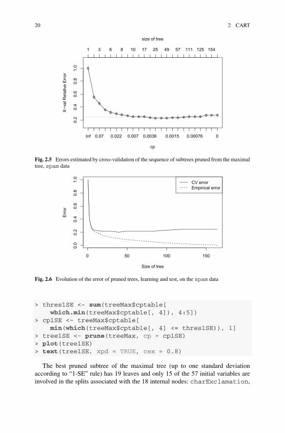
and the generalization errors of the corresponding trees T1, . . . , TK . In the graphof Fig. 2.5 obtained on the spam data (see p. 20), each point represents a tree:the abscissa is placed according to the value of the corresponding αk , the ordinateaccording to the error estimated by cross-validation with the estimation of the stan-dard deviation of the error materialized by a vertical segment.
The choice of the optimal tree can be made directly, by minimizing the errorobtained by cross-validation or by applying the “1 standard error rule” (“1-SE rule”in brief). This rule aims at selecting in the sequence a more compact tree reachingstatistically the same error. It consists in choosing the most compact tree reachingan error lower than the value of the previous minimum augmented by the estimatedstandard error of this error. This quantity is represented by the horizontal dotted lineon the example of Fig. 2.5.
Remark 2.2 The cross-validation procedure (V -fold cross-validation), executed bydefault in the rpart package is as follows. First, starting from Ln and applyingthe pruning algorithm, we obtain the sequences (Tk)1≤k≤K and (αk)1≤k≤K . Then,the learning sample is randomly divided into subsamples (often V = 10) so thatLn = E1 ∪ E2 ∪ · · · ∪ EV . For each v = 1, . . . , V , we build the sequence of subtrees(T v
k )1≤k≤KvwithLn \ Ev as learning sample. Then we calculate the validation errors
of the sequence of trees built on Ln: Rcv(Tk) = 1V
∑Vv=1
∑
(xi ,yi )∈Ev
(
yi − T vk (xi )
)2,

16 2 CART
where T vk minimizes the penalized criterion critα′
k, with α′
k = (αkαk+1)1/2.We finally
choose the model Tk where k = argmin1≤k≤K Rcv(Tk).Let us mention that the choice of α by a validation sample is not available in the
rpart package.
Finally, it should be noted that, of course, if a tree in the sequence has k leaves, itis the best tree with k leaves. On the other hand, this sequence does not necessarilycontain all the best trees with k leaves for 1 ≤ k ≤ |Tmax| but only a part of them.However, the “missing” trees are simply not competitive because they correspond tolarger values of the penalized criterion, so it is useless to calculate them. In additiontheir calculation could be more expensive since they are not, in general, pruned fromthe trees of the sequence.
As we will see below, random forests are, in most cases, forests of unpruned trees.However, it should be stressed that a CART tree, if it used alone, must be pruned.Otherwise, it would suffer from overfitting by being too adapted to the data in Ln
and exhibit a too large generalization error.
2.4 The rpart Package
The rpart package (Therneau and Atkinson 2018) implements the CART methodas a whole and is installed by default in R. The rpart() function allows to build atree whose development is controlled by the parameters of the rpart.control()function and pruning is achieved through the prune() function. Finally, the meth-odsprint(),summary(),plot(), and predict() allow retrieving and illus-trate the results. It should also be noted that rpart fully handles missing data, bothfor prediction (see Sect. 2.5.2) and for learning (see details on the Ozone examplein Sect. 2.6.1).
Other packages that implement decision trees are used in R, such as
• tree (Ripley 2018), quite close to rpart but which allows, for example, to tracethe partition associated with a tree in small dimension and use a validation samplefor pruning.
• rpart.plot (Milborrow 2018) which offers advanced graphics functions.• party (Hothorn et al. 2017) which proposes other criteria for optimizing the split-ting of a node.
Now let us detail the use of the functions rpart() and prune() on the spamdetection example.
The tree built with the default values of rpart() is obtained as follows. Notethat only the syntax formula =, data = is allowed for this function.
> library(rpart)> treeDef <- rpart(type ˜ ., data = spamApp)> print(treeDef, digits = 2)

2.4 The rpart Package 17
n= 2300
node), split, n, loss, yval, (yprob)* denotes terminal node
1) root 2300 910 ok (0.606 0.394)2) charExclamation< 0.08 1369 230 ok (0.834 0.166)
4) remove< 0.045 1263 140 ok (0.892 0.108)8) money< 0.15 1217 100 ok (0.917 0.083) *9) money>=0.15 46 11 spam (0.239 0.761) *
5) remove>=0.045 106 15 spam (0.142 0.858) *3) charExclamation>=0.08 931 250 spam (0.271 0.729)
6) charDollar< 0.0065 489 240 spam (0.489 0.511)12) capitalAve< 2.8 307 100 ok (0.674 0.326)
24) remove< 0.09 265 60 ok (0.774 0.226)48) free< 0.2 223 31 ok (0.861 0.139) *49) free>=0.2 42 13 spam (0.310 0.690) *
25) remove>=0.09 42 2 spam (0.048 0.952) *13) capitalAve>=2.8 182 32 spam (0.176 0.824)
26) hp>=0.1 14 2 ok (0.857 0.143) *27) hp< 0.1 168 20 spam (0.119 0.881) *
7) charDollar>=0.0065 442 13 spam (0.029 0.971) *
> plot(treeDef)> text(treeDef, xpd = TRUE)
The print() method allows to obtain a text representation of the obtaineddecision tree, and the sequence of methods plot() then text() give a graphicalrepresentation (Fig. 2.4).
Remark 2.3 Caution, contrary to what one might think, the tree obtained with thedefault values of the package is not an optimal tree in the pruning sense. In fact, itis a tree whose development has been stopped, thanks to the parameters minsplit(the minimum number of data in a node necessary for the node to be possiblysplit) and cp (the normalized complexity-penalty parameter), documented in therpart.control() function help page. Thus, as cp = 0.01 by default, thetree provided corresponds to the one obtained by selecting the one correspondingto α = 0.01 ∗ err(Tn) (where T1 is the root), provided that minsplit is not theparameter that stops the tree development. It is therefore not the optimal tree butgenerally a more compact one.
The maximal tree is then obtained using the following command (using theset.seed() function to ensure reproducibility of cross-validation results):
> set.seed(601334)> treeMax <- rpart(type ˜ ., data = spamApp, minsplit = 2, cp = 0)> plot(treeMax)
The application of the plot()method allows to obtain the skeleton of the max-imal tree (Fig. 2.3).

18 2 CART
|charExclamation< 0.0795
remove< 0.045
money< 0.145
charDollar< 0.0065capitalAve< 2.752
remove< 0.09
free< 0.2
hp>=0.105ok spam
spam
ok spamspam
ok spam
spam
Fig. 2.4 Classification tree obtained with the default values of rpart(), spam data
Information on the optimal sequence of the pruned subtrees of Tmax obtained byapplying the pruning algorithm is given by the command:
> treeMax$cptable
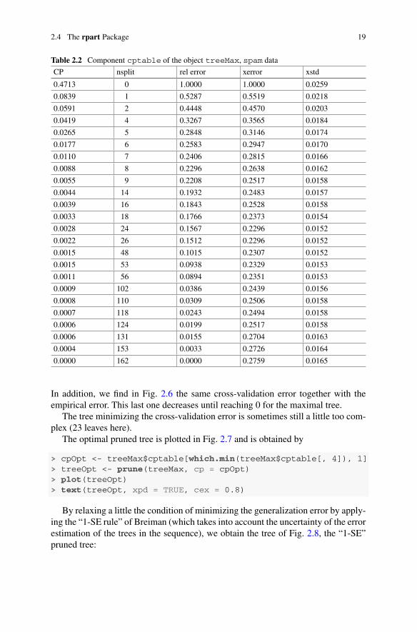
In the columns of Table 2.2, we find the value of the penalty parameter, the numberof splits of the corresponding optimal tree, the relative empirical error with respectto the one made by the tree restricted to the root, then the relative cross-validationerror, and an estimate of the standard deviation of the associated estimator.
More graphically, we can visualize the sequence of the pruned subtrees of Tmax
(Fig. 2.5), thanks to the plotcp() function:
> plotcp(treeMax)
Each point thus represents a tree, with the estimation of the standard deviationof the cross-validation error as a vertical segment, quite hard to distinguish on thisexample (see Fig. 2.11 for a more meaningful graph). The position of the pointindicates on the y-axis the (relative) cross-validation error, on the bottom x-axis thevalue of the penalty parameter, and on the top x-axis the number of leaves of the tree.
The shape of this graph is typical. Let us read it from left to right. When the modelis too simple, the bias dominates and the error is significant. Then, it decreasesfairly quickly until it reaches a minimum reflecting a good balance between biasand variance and finally rises slightly as the complexity of the model increases.
2.4 The rpart Package 19
Table 2.2 Component cptable of the object treeMax, spam data
CP nsplit rel error xerror xstd
0.4713 0 1.0000 1.0000 0.0259
0.0839 1 0.5287 0.5519 0.0218
0.0591 2 0.4448 0.4570 0.0203
0.0419 4 0.3267 0.3565 0.0184
0.0265 5 0.2848 0.3146 0.0174
0.0177 6 0.2583 0.2947 0.0170
0.0110 7 0.2406 0.2815 0.0166
0.0088 8 0.2296 0.2638 0.0162
0.0055 9 0.2208 0.2517 0.0158
0.0044 14 0.1932 0.2483 0.0157
0.0039 16 0.1843 0.2528 0.0158
0.0033 18 0.1766 0.2373 0.0154
0.0028 24 0.1567 0.2296 0.0152
0.0022 26 0.1512 0.2296 0.0152
0.0015 48 0.1015 0.2307 0.0152
0.0015 53 0.0938 0.2329 0.0153
0.0011 56 0.0894 0.2351 0.0153
0.0009 102 0.0386 0.2439 0.0156
0.0008 110 0.0309 0.2506 0.0158
0.0007 118 0.0243 0.2494 0.0158
0.0006 124 0.0199 0.2517 0.0158
0.0006 131 0.0155 0.2704 0.0163
0.0004 153 0.0033 0.2726 0.0164
0.0000 162 0.0000 0.2759 0.0165
In addition, we find in Fig. 2.6 the same cross-validation error together with theempirical error. This last one decreases until reaching 0 for the maximal tree.
The tree minimizing the cross-validation error is sometimes still a little too com-plex (23 leaves here).
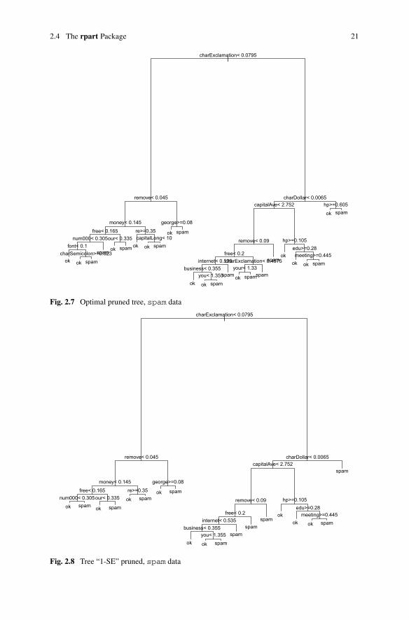
The optimal pruned tree is plotted in Fig. 2.7 and is obtained by
> cpOpt <- treeMax$cptable[which.min(treeMax$cptable[, 4]), 1]> treeOpt <- prune(treeMax, cp = cpOpt)> plot(treeOpt)> text(treeOpt, xpd = TRUE, cex = 0.8)
By relaxing a little the condition of minimizing the generalization error by apply-ing the “1-SE rule” of Breiman (which takes into account the uncertainty of the errorestimation of the trees in the sequence), we obtain the tree of Fig. 2.8, the “1-SE”pruned tree:
20 2 CART
cp
X−va
l Rel
ativ
e Er
ror
0.2
0.4
0.6
0.8
1.0
Inf 0.07 0.022 0.007 0.0036 0.0015 0.00076 0
1 3 6 8 10 17 25 49 57 111 125 154
size of tree
Fig. 2.5 Errors estimated by cross-validation of the sequence of subtrees pruned from the maximaltree, spam data
0 50 100 150
0.0
0.2
0.4
0.6
0.8
1.0
Size of tree
Erro
r
CV errorEmpirical error
Fig. 2.6 Evolution of the error of pruned trees, learning and test, on the spam data
> thres1SE <- sum(treeMax$cptable[which.min(treeMax$cptable[, 4]), 4:5])
> cp1SE <- treeMax$cptable[min(which(treeMax$cptable[, 4] <= thres1SE)), 1]
> tree1SE <- prune(treeMax, cp = cp1SE)> plot(tree1SE)> text(tree1SE, xpd = TRUE, cex = 0.8)
The best pruned subtree of the maximal tree (up to one standard deviationaccording to “1-SE” rule) has 19 leaves and only 15 of the 57 initial variables areinvolved in the splits associated with the 18 internal nodes: charExclamation,
2.4 The rpart Package 21
|charExclamation< 0.0795
remove< 0.045
money< 0.145free< 0.165
num000< 0.305font< 0.1
charSemicolon>=0.023
our< 0.335re>=0.35capitalLong< 10
george>=0.08
charDollar< 0.0065capitalAve< 2.752
remove< 0.09
free< 0.2internet< 0.535
business< 0.355you< 1.355
charExclamation< 0.4575your< 1.33
hp>=0.105edu>=0.28meeting>=0.445
hp>=0.605
ok ok spam
spam ok spam ok ok spam
ok spam
ok ok spam
spam ok spamspam
spamok
ok ok spam
ok spam
Fig. 2.7 Optimal pruned tree, spam data
|charExclamation< 0.0795
remove< 0.045
money< 0.145free< 0.165
num000< 0.305our< 0.335re>=0.35
george>=0.08
charDollar< 0.0065capitalAve< 2.752
remove< 0.09
free< 0.2internet< 0.535
business< 0.355you< 1.355
hp>=0.105edu>=0.28
meeting>=0.445ok spam ok spam
ok spamok spam
ok ok spam
spamspam
spamok
ok ok spam
spam
Fig. 2.8 Tree “1-SE” pruned, spam data
22 2 CART
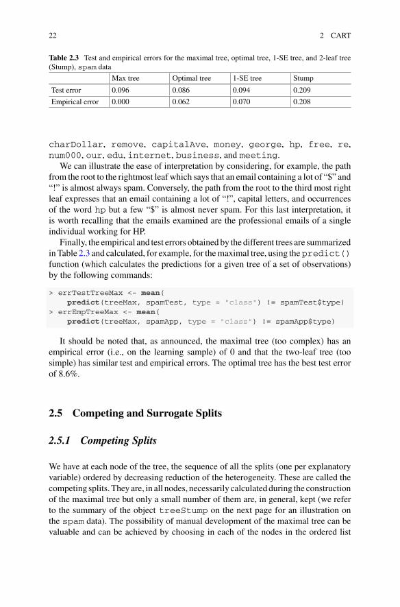
Table 2.3 Test and empirical errors for the maximal tree, optimal tree, 1-SE tree, and 2-leaf tree(Stump), spam data
Max tree Optimal tree 1-SE tree Stump
Test error 0.096 0.086 0.094 0.209
Empirical error 0.000 0.062 0.070 0.208
charDollar, remove, capitalAve, money, george, hp, free, re,num000, our, edu, internet, business, and meeting.
We can illustrate the ease of interpretation by considering, for example, the pathfrom the root to the rightmost leaf which says that an email containing a lot of “$” and“!” is almost always spam. Conversely, the path from the root to the third most rightleaf expresses that an email containing a lot of “!”, capital letters, and occurrencesof the word hp but a few “$” is almost never spam. For this last interpretation, itis worth recalling that the emails examined are the professional emails of a singleindividual working for HP.
Finally, the empirical and test errors obtained by the different trees are summarizedin Table 2.3 and calculated, for example, for themaximal tree, using the predict()function (which calculates the predictions for a given tree of a set of observations)by the following commands:
> errTestTreeMax <- mean(predict(treeMax, spamTest, type = "class") != spamTest$type)
> errEmpTreeMax <- mean(predict(treeMax, spamApp, type = "class") != spamApp$type)
It should be noted that, as announced, the maximal tree (too complex) has anempirical error (i.e., on the learning sample) of 0 and that the two-leaf tree (toosimple) has similar test and empirical errors. The optimal tree has the best test errorof 8.6%.
2.5 Competing and Surrogate Splits
2.5.1 Competing Splits
We have at each node of the tree, the sequence of all the splits (one per explanatoryvariable) ordered by decreasing reduction of the heterogeneity. These are called thecompeting splits. They are, in all nodes, necessarily calculatedduring the constructionof the maximal tree but only a small number of them are, in general, kept (we referto the summary of the object treeStump on the next page for an illustration onthe spam data). The possibility of manual development of the maximal tree can bevaluable and can be achieved by choosing in each of the nodes in the ordered list

2.5 Competing and Surrogate Splits 23
of splits, either the optimal one, or a slightly worse split. The actual split variablecould be less uncertain, easier, cheaper to measure, or even more interpretable (see,for example, Ghattas 2000).
2.5.2 Surrogate Splits
One of the practical difficulties in calculating a prediction is the presence of missingvalues. CART offers an effective and very elegant way to circumvent it. First of all,it should be noted that when some input variables are missing for a given x , there is aproblem only if the path to calculate the predicted value goes through a node whosesplit is based on one of these variables. Then, in a node where the split variable ismissing, one of the other variables can be used, for example, the second competingsplit. But this idea is not optimal, since the routing rule in the right and left nodes,respectively, can be very different from the routing rule induced by the optimal split.Hence, the idea is to calculate at each node the list of surrogate splits, defined bythe splits minimizing the number of routing errors with respect to the routing ruleinduced by the optimal split. This provides a method for handling missing values forprediction that is both local and efficient, avoiding to use global and often too coarseimputation methods.
These two aspects are illustrated by the following instructions.
> treeStump <- rpart(type ˜ ., data = spamApp, maxdepth = 1)> summary(treeStump)
Call:rpart(formula = type ˜ ., data = spamApp, maxdepth = 1)
n= 2300
CP nsplit rel error xerror xstd1 0.4713024 0 1.0000000 1.0000000 0.025864462 0.0100000 1 0.5286976 0.5474614 0.02177043
Variable importancecharExclamation free your charDollar
44 12 12 12capitalLong all
11 10
Node number 1: 2300 observations, complexity param=0.4713024predicted class=ok expected loss=0.393913 P(node) =1
class counts: 1394 906probabilities: 0.606 0.394
left son=2 (1369 obs) right son=3 (931 obs)Primary splits:

24 2 CART
charExclamation < 0.0795 to the left, improve=351.9304charDollar < 0.0555 to the left, improve=337.1138free < 0.095 to the left, improve=296.6714remove < 0.01 to the left, improve=290.1446your < 0.605 to the left, improve=272.6889
Surrogate splits:free < 0.135 to the left, agree=0.710, adj=0.285your < 0.755 to the left, agree=0.703, adj=0.267charDollar < 0.0555 to the left, agree=0.702, adj=0.264capitalLong < 53.5 to the left, agree=0.694, adj=0.245all < 0.325 to the left, agree=0.685, adj=0.221
Node number 2: 1369 observationspredicted class=ok expected loss=0.1658145 P(node) =0.5952174
class counts: 1142 227probabilities: 0.834 0.166
Node number 3: 931 observationspredicted class=spam expected loss=0.2706767 P(node) =0.4047826
class counts: 252 679probabilities: 0.271 0.729
This tree is the default tree of depth 1 (called stump), a typical weak classifier.The result of the method summary() provides information not only about thevisible parts of the tree (such as structure and splits) but also about the hidden parts,involving variables that do not necessarily appear in the selected tree. Thus, we firstfind competing splits and then surrogate splits. It should be noted that to mimic theoptimal routing rule, the best alternative split isfree < 0.135which differs fromthe competing split based on the same variable that is free < 0.095.
2.5.3 Interpretability
The interpretability of CART trees is one of the ingredients of their success. It isindeed very easy to answer the question of why, for a given x , a particular value ofy is expected. To do this, it suffices to provide the sequence of the answers to thequestions constituted by the successive splits encountered to go through the onlypath from the root to the associated leaf.
But more generally, beyond the interpretation of a particular prediction, once theCART tree has been built, we can consider the variables that intervene in the splits ofthe nodes of the tree. It is natural to think that the variables involved in splits close tothe root are the most important, since they correspond to those whose contribution tothe heterogeneity reduction is important. In a complementary way, we would tend tothink that the variables that do not appear in any split are not important. Actually, thisfirst intuition gives partial and biased results. Indeed, variables that do not appearin the tree can be important and even useful in this same model to deal with theproblem of missing data in prediction, for example. A more sophisticated variable

2.5 Competing and Surrogate Splits 25
importance index is provided by CART trees. It is based on the concept of surrogatesplits. According to Breiman et al. (1984), the importance of a variable can be definedby evaluating, in each node, the heterogeneity reduction generated by the use of thesurrogate split for that variable and then summing them over all nodes.
In rpart, the importance of the variable X j is defined by the sum of two terms.The first is the sum of the heterogeneity reductions generated by the splits involvingX j , and the second is weighted the sum of the heterogeneity reductions generatedby the surrogate splits when X j does not define the split. In the second case, theweighting is equal to the relative agreement, in excess of the majority routing rule,given for a node t of size nt , by
{
(nX j − nmaj)/(nt − nmaj) if nX j > nmaj
0 otherwise
where nX j and nmaj are the numbers of observations well routed with respect to theoptimal split of the node t , respectively, by the surrogate split involving X j and bythe split according to the majority rule (which routes all observations to the childnode of largest size). This weighting reflects the adjusted relative agreement betweenthe optimal routing rule and the one associated with the surrogate split involving X j ,in excess of the majority rule. The raw relative agreement would be simply given bynX j /nt .
However, as interesting as this variable importance indexmay be, it is no longer sowidely used today. It is indeed not very intuitive, it is unstable because it is stronglydependent on a given tree, and it is less relevant than the importance of variables bypermutation in the sense of random forests. In addition, its analog, which does notuse surrogate splits, exists for random forests but tends to favor nominal variablesthat have a large number of possible values (we will come back to this in Sect. 4.1).
> par(mar = c(7, 3, 1, 1) + 0.1)> barplot(treeMax$variable.importance, las = 2, cex.names = 0.8)
Nevertheless, it can be noted that the variable importance indices, in the sense ofCART, for the maximal tree (given by Fig. 2.9) provide for the spam detection exam-ple very reasonable and easily interpretable results. It makes it possible to identifya group of variables: charExclamation clearly at the top then capitalLong,charDollar, free and remove then, less clearly, a group of 8 variables amongwhich capitalAve, capitalTotal, money but also your and num000 intu-itively less interesting.

26 2 CART
char
Excl
amat
ion
capi
talL
ong
char
Dol
lar
free
rem
ove
capi
talA
veyo
urca
pita
lTot
al all
mon
eynu
m00
0yo
u hp will
edu
our
busi
ness
geor
gech
arSe
mic
olon
char
Has
hnu
m65
0hp
lm
ake
inte
rnet
char
Rou
ndbr
acke
tad
dres
sre
ceiv
enu
m85
repo
rtnu
m41
5ov
erem
ail
lab
font
mai
lpm
num
857
cred
it repr
ojec
tor
igin
alm
eetin
gla
bsnu
m19
99da
tate
chno
logy
addr
esse
sch
arSq
uare
brac
ket
teln
etor
der
peop
ledi
rect
parts
conf
eren
ce
0
50
100
150
200
250
300
350
Fig. 2.9 Importance of variables in the sense of CART for the maximal tree, spam data
2.6 Examples
2.6.1 Predicting Ozone Concentration
For a presentation of this dataset, see Sect. 1.5.2.Let us load the rpart package and the Ozone data:
> library("rpart")> data("Ozone", package = "mlbench")
Let us start by building a tree using the default values of rpart():
> OzTreeDef <- rpart(V4 ˜ ., data = Ozone)> plot(OzTreeDef)> text(OzTreeDef, xpd = TRUE, cex = 0.9)
Note that the response variable is in column 4 of the data Table and is denoted byV4.
Let us analyze this first tree (Fig. 2.10). This dataset has already been consideredin many studies and, although these are real data, the results are relatively easy tointerpret.
Looking at the first splits in the tree, we notice that the variables V8, V10 thenV1 and V2 define them. Let us explain why.
Ozone is a secondary pollutant, since it is produced by the chemical transformationof primary precursor gases generated directly from the exhaust pipes (hydrocarbonsand nitrogen oxides) in the presence of a catalyst for the chemical reaction: ultraviolet

2.6 Examples 27
|V8< 67.5
V10>=3574
V1=al
V2=abcfhjnpqrswxCD
V5< 5735
V8< 79.5
V2=bcdefhiklopsvwCDE
V11< −13.5
V12< 73.04
V2=abhijknorwxyzAE5.07
5.424
8.93 10.56 15.48 6.125 14.21 20.75
20.2921.12 28.05
Fig. 2.10 Default tree, Ozone data
radiation. The latter is highly correlated with temperature (V8 or V9), which is oneof the most important predictors of ozone. As a result, ozone concentrations peakduring the summer months and this explains why the month number (V1) is amongthe influential variables. Finally, above an agglomeration, the pollutants are dispersedin a box whose base is the agglomeration and whose height is given by the inversionbase height (V10).
Continuing to explore the tree, we notice that V2 defines splits quite close to theroot of the tree, despite the fact that V2 is the number of the day within the monthwhose relationshipwith the response variable can only be caused by sampling effects.The explanation is classical in tree-based methods: it comes from the fact that V2 is anominal variable with many possible values (here 31) involving a favorable selectionbias when choosing the best split.
Predictions can also be easily interpreted: for example, the leftmost leaf gives verylow predictions because it corresponds to cold days with a high inversion base height.On the other hand, the rightmost leaf provides much larger predictions because itcorresponds to hot days.
Of course, it is now necessary to optimize the choice of the final tree. Let us studyfor that the sequence of the pruned subtrees (Fig. 2.11) which is the result of thepruning step starting from the the maximal tree.
> set.seed(727325)> OzTreeMax <- rpart(V4 ˜ ., data = Ozone, minsplit = 2, cp = 0)> plotcp(OzTreeMax)

28 2 CART
cp
X−va
l Rel
ativ
e Er
ror
0.4
0.6
0.8
1.0
1.2
Inf 0.0076 0.0023 0.001 0.00044 0.00027 1e−04 3.6e−05
1 8 18 28 38 50 60 70 80 94 109 130 150 167
size of tree
Fig. 2.11 Errors estimated by cross-validation of the sequence of subtrees pruned from themaximaltree, Ozone data
> OzIndcpOpt <- which.min(OzTreeMax$cptable[, 4])> OzcpOpt <- OzTreeMax$cptable[OzIndcpOpt, 1]> OzTreeOpt <- prune(OzTreeMax, cp = OzcpOpt)> plot(OzTreeOpt)> text(OzTreeOpt, xpd = TRUE)
The best tree (Fig. 2.12) is particularly compact since it has only six leaves, thoseinvolving splits on twoof the threemajor variables highlighted above.Wewill see thata more complete, but above all, more automatic exploration of this aspect is providedby the permutation variable importance index in the context of random forests. Thisnotion will allow eliminating the variable V2 whose interest is doubtful.
There is a lot of missing data in this dataset and rpart() offers a clever way tohandle it during the learning step, without any imputation:
• The data with y missing are eliminated as well as those with all the componentsof x missing.
• Otherwise, to split a node:
– Calculate the impurity reductions for each variable using only the associatedavailable data and choose the best split as usual.
– For this split, observations that have a missing value for the associated splitvariable are routed, either using a surrogate split or to the most popular node incase the variables determining the best available surrogate splits are all missingfor this observation (the maximum number is a parameter, set to 5 by default).
– Finally, weights in the impurity reduction are updated to take into account thenew data routed.

2.6 Examples 29
|V8< 67.5
V10>=3574
V1=al
V8< 79.5
V2=bcdefhiklopsvwCDE5.07
5.424 11.07 13.96 20.2924.11
Fig. 2.12 Optimal pruned tree, Ozone data
2.6.2 Analyzing Genomic Data
For a presentation of this dataset, see Sect. 1.5.3.Let us load the rpart package, the vac18 data, and group in the same dataframe
in which the gene expressions and the stimulation are to be predicted:
> library(rpart)> data("vac18", package = "mixOmics")> VAC18 <- data.frame(vac18$genes, stimu = vac18$stimulation)
The tree obtainedwith the default values of rpart() is obtained as follows (notethe use of the argument use.n = TRUE in the text() function which displaysthe class distribution for each leaf):
> VacTreeDef <- rpart(stimu ˜ ., data = VAC18)> VacTreeDef
n= 42
node), split, n, loss, yval, (yprob)* denotes terminal node
1) root 42 31 LIPO5 (0.262 0.238 0.238 0.262)2) ILMN_2136089>=9.05 11 0 LIPO5 (1.000 0.000 0.000 0.000) *3) ILMN_2136089< 9.05 31 20 NS (0.000 0.323 0.323 0.355)
6) ILMN_2102693< 8.59 18 8 GAG+ (0.000 0.556 0.444 0.000)*7) ILMN_2102693>=8.59 13 2 NS (0.000 0.000 0.154 0.846) *

30 2 CART
|ILMN_2136089>=9.055
ILMN_2102693< 8.59LIPO511/0/0/0
GAG+ 0/10/8/0
NS0/0/2/11
Fig. 2.13 Default tree obtained with rpart() on the Vac18 data
> plot(VacTreeDef)> text(VacTreeDef, use.n = TRUE, xpd = TRUE)
The default tree, represented in Fig. 2.13, consists of only 3 leaves. This is due,on the one hand, to the fact that there are only 42 observations in the dataset, and,on the other hand, that the classes LIPO5 and NS are separated from the others veryquickly. Indeed, that the first split sends all the observations of class LIPO5, andonly them, to the left child node.
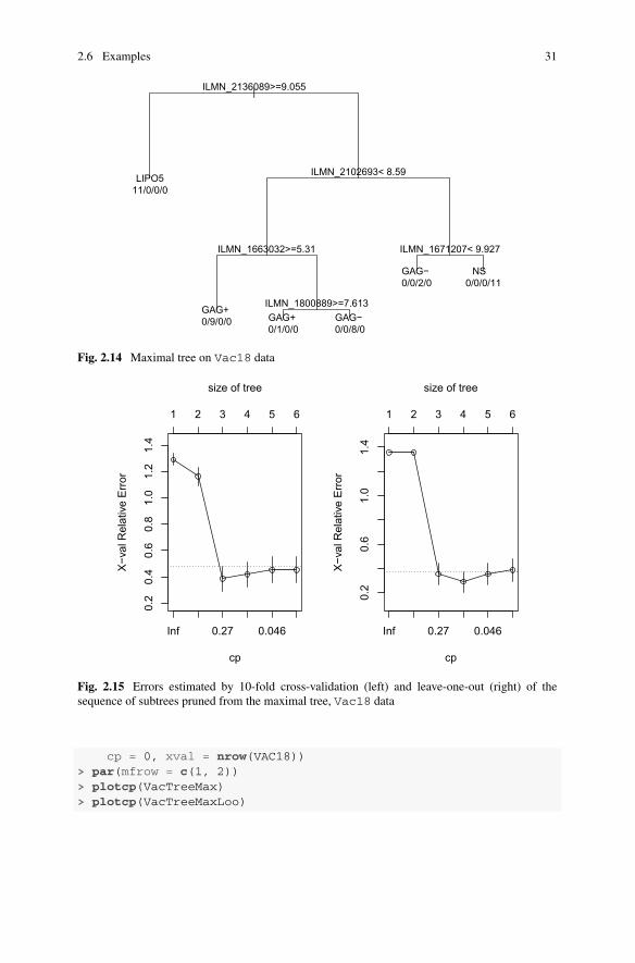
Themaximal tree has 6 leaves (Fig. 2.14). Thus in 5 splits, the classes are perfectlyseparated. We see on this example that considering only the variables appearing inthe splits of a tree (here the deepest tree which can be built using these data) canbe very restrictive: indeed, only 5 variables (corresponding to probe identifiers ofbiochips) among the 1,000 variables appear in the tree.
> set.seed(788182)> VacTreeMax <- rpart(stimu ˜ ., data = VAC18, minsplit = 2, cp = 0)> plot(VacTreeMax)> text(VacTreeMax, use.n = TRUE, xpd = TRUE)
The error estimated by validation for the sequence of pruned subtrees is plottedin the left graph of Fig. 2.15.
Given the small number of individuals, a leave-one-out estimate of the cross-validation error may be preferred. This is obtained by setting the argument xval,the number of folds of the cross-validation (argument of the rpart.control()function), as follows:
> set.seed(413745)> VacTreeMaxLoo <- rpart(stimu ˜ ., data = VAC18, minsplit = 2,
2.6 Examples 31
|ILMN_2136089>=9.055
ILMN_2102693< 8.59
ILMN_1663032>=5.31
ILMN_1800889>=7.613
ILMN_1671207< 9.927
LIPO511/0/0/0
GAG+ 0/9/0/0 GAG+
0/1/0/0GAG− 0/0/8/0
GAG− 0/0/2/0
NS0/0/0/11
Fig. 2.14 Maximal tree on Vac18 data
cp
X−va
l Rel
ativ
e Er
ror
size of tree
cp
X−va
l Rel
ativ
e Er
ror
0.2
0.4
0.6
0.8
1.0
1.2
1.4
0.2
0.6
1.0
1.4
Inf 0.27 0.046
1 2 3 4 5 6
Inf 0.27 0.046
1 2 3 4 5 6
size of tree
Fig. 2.15 Errors estimated by 10-fold cross-validation (left) and leave-one-out (right) of thesequence of subtrees pruned from the maximal tree, Vac18 data
cp = 0, xval = nrow(VAC18))> par(mfrow = c(1, 2))> plotcp(VacTreeMax)> plotcp(VacTreeMaxLoo)

32 2 CART
|ILMN_2136089>=9.055
ILMN_2102693< 8.59
ILMN_1663032>=5.31
LIPO511/0/0/0
GAG+ 0/9/0/0
GAG− 0/1/8/0
NS0/0/2/11
Fig. 2.16 Optimal pruned tree, Vac18 data
We can easily see on the right side of Fig. 2.15 that for leave-one-out cross-validation, the optimal tree consists of 4 leaves while the 1-SE tree is the same as thedefault tree (3 leaves). The optimal tree (Fig. 2.16) is obtained using the followingcommands:
> VacIndcpOpt <- which.min(VacTreeMaxLoo$cptable[, 4])> VaccpOpt <- VacTreeMaxLoo$cptable[VacIndcpOpt, 1]> VacTreeOpt <- prune(VacTreeMaxLoo, cp = VaccpOpt)> plot(VacTreeOpt)> text(VacTreeOpt, use.n = TRUE, xpd = TRUE)

Chapter 3Random Forests
Abstract The general principle of random forests is to aggregate a collection ofrandom decision trees. The goal is, instead of seeking to optimize a predictor “atonce” as for a CART tree, to pool a set of predictors (not necessarily optimal). Sinceindividual trees are randomly perturbed, the forest benefits from a more extensiveexploration of the space of all possible tree predictors, which, in practice, resultsin better predictive performance. Focusing on random forests, this chapter beginsby addressing the instability of a tree and subsequently introduces readers to tworandom forest variants: Bagging and Random Forest Random Inputs. The construc-tion of random forests is illustrated on the spam dataset using the randomForestpackage. The clever prediction error estimate Out-Of-Bag Error is also presented. Inturn, the chapter assesses the sensitivity of prediction performance to the two mainparameters: the number of trees and the number of variables picked at each node.In the final section, random forests are applied to three examples: predicting ozoneconcentration, analyzing genomic data, and analyzing dust pollution.
3.1 General Principle
The general principle of random forests (RF henceforth) is to aggregate a collectionof random decision trees. The goal is, instead of seeking to optimize a predictor “atonce” as for a CART tree, to pool a set of predictors (not necessarily optimal). Sinceindividual trees are randomly perturbed, the forest benefits from a more extensiveexploration of the space of all possible tree predictors, which, in practice, results inbetter predictive performance.
The general definition of random forests, given by Breiman (2001), is as follows:
Definition 3.1 (Random forests) Let(h(.,Θ1), . . . , h(.,Θq)
)be a collection of tree
predictors, withΘ1, . . . , Θq q i.i.d. randomvariables independent ofLn . The randomforest predictor h RF is obtained by aggregating this collection of random trees. Theaggregation is done as follows:
© Springer Nature Switzerland AG 2020R. Genuer and J.-M. Poggi, Random Forests with R, Use R!,https://doi.org/10.1007/978-3-030-56485-8_3
33

34 3 Random Forests
Fig. 3.1 General scheme ofrandom forests
• h RF (x) = 1
q
q∑
�=1
h(x,Θ�) (average of individual tree predictions) in regression.
• h RF (x) = argmax1≤c≤C
q∑
�=1
1h(x,Θ�)=c (majority vote among individual tree predictions)
in classification.
Remark 3.1 Actually, this definition is not exactly the same as that of Breiman(2001), which does not specify that the variables� are independent ofLn . However,we adopt Definition 3.1 in this book because we find it more appropriate. Indeed, itis consistent with the intuition that the additional randomness provided by the �
is disconnected from the learning sample and, in addition, it encompasses the mostcommonly used RF variants.
This definition is illustrated by the diagram in Fig. 3.1. This scheme will beadapted several times later in this chapter, depending on the different RF methodspresented.
In order to obtain good predictive performance, a random forest method mustbuild a collection of trees that is
• As diverse as possible, because aggregating a set of predictors that are all verysimilar would give nothing more than again a similar predictor.
• Made up of individual predictors with acceptable predictive capacity, because iffor a new observation x all trees provide a bad prediction, the aggregation of thesepredictions has no chance of being correct.
3.1.1 Instability of a Tree
Before presenting differentRFvariants,we illustrate awell-knownproperty ofCARTtrees, namely their instability. Instability here means that if the learning sample onwhich a CART tree is built is slightly modified, then the resulting tree is usually verydifferent from the original tree.

3.1 General Principle 35
To illustrate this behavior, let us build two CART trees (with parameter defaultvalues of the rpart() function) from two different bootstrap samples, namedspamBoot1 and spamBoot2, derived from the spam data learning sample,spamApp. The notion of bootstrap samples is introduced in the following definition.
Definition 3.2 (Bootstrap sample) A bootstrap sample of a learning sample Ln ofsize n is obtained by randomly drawing n observations from Ln with replacement,each observation (Xi ,Yi ) of Ln having a probability 1/n of being selected in eachdraw.
> set.seed(368910)> spamBoot1 <- spamApp[
sample(1:nrow(spamApp), nrow(spamApp), replace = TRUE), ]> treeBoot1 <- rpart(type ˜ ., data = spamBoot1)> plot(treeBoot1)> text(treeBoot1, xpd = TRUE)
> set.seed(368915)> spamBoot2 <- spamApp[
sample(1:nrow(spamApp), nrow(spamApp), replace = TRUE), ]> treeBoot2 <- rpart(type ˜ ., data = spamBoot2)> plot(treeBoot2)> text(treeBoot2, xpd = TRUE)
We note that the structures of the two trees (Figs. 3.2 and 3.3) are very different.This major difference is explained by the fact that, as illustrated, there are changesfrom the first splits (at the top of the tree). Thus, the recursive nature of CART treebuilding implies that these changes are reflected throughout the tree development. Inaddition, since the pruning step is conditional on the maximal tree, the differencesobserved would be as important for pruned trees.
If we compare them with the tree obtained in Fig. 2.4, we notice that the treebuilt on the sample spamBoot2 is relatively similar to the one built on the wholelearning sample spamApp. Thus, depending on the bootstrap sample, resulting treescould be very different from each other.
Finally, we could expect to see the variable charDollar appear in the rootnode split in such a situation, because in Sect. 2.5 we saw that it occurred in the firstconcurrent split of this node, with a value of improve relatively close to that of theoriginal split (made on the variable charExclamation).
Now let us compare predictions given by the two previous trees on the test sample.
> mean(predict(treeBoot1, spamTest, type = "class") !=predict(treeBoot2, spamTest, type = "class"))
[1] 0.08822251

36 3 Random Forests
|charDollar< 0.0335
remove< 0.06
free< 0.225
charExclamation< 0.326capitalAve< 2.295
charExclamation< 0.289capitalLong>=48.5
george>=0.34
hp>=0.24
okok spam ok ok spam
spam
spam
ok spam
Fig. 3.2 Classification tree obtained with the default values of rpart() on the bootstrap samplespamBoot1; spam data
|charExclamation< 0.079
remove< 0.025
money< 0.165
will< 0.235
charDollar< 0.0065
remove< 0.07
capitalAve< 2.752
free< 0.495ok ok spam
spam
ok spamspam
spam
spam
Fig. 3.3 Classification tree obtained with the default values of rpart() on the bootstrap samplespamBoot2, spam data

3.1 General Principle 37
This result illustrates that the instability of CART trees also results in a variationof predictions. In our example, about 8.8% of the test data has an altered prediction.
3.1.2 From a Tree to an Ensemble: Bagging
The first historical example of a random forest method that verifies the conditionsof Definition 3.1 is the Bagging method introduced by Breiman (1996). The wordBagging is the acronym for “Bootstrap aggregating”. Thus, the Bagging predictoris obtained by aggregating a set of tree predictors, each constructed on a differentbootstrap sample. This method is therefore a random forest where the hazard comesfrom the bootstrap draw.
The diagram of Fig. 3.4 summarizes the principle of Bagging.To illustrate Bagging on spam data, we can use the randomForest package,
presented in detail in Sect. 3.3.The Bagging predictor is obtained using the following command, for which the
mtry parameter of the randomForest() function is set to p, the number ofexplanatory variables, while all other parameters are kept to their default values. Wewill come back to the meaning of the mtry parameter in Sect. 3.2.
> library(randomForest)> bagging <- randomForest(type ˜ ., data = spamApp,
mtry = ncol(spamApp) - 1)> bagging
Call:
Fig. 3.4 Bagging diagram

38 3 Random Forests
randomForest(formula = type ˜ ., data = spamApp,
mtry = ncol(spamApp) - 1)
Type of random forest: classification
Number of trees: 500
No. of variables tried at each split: 57
OOB estimate of error rate: 6.13%
Confusion matrix:
ok spam class.error
ok 1339 55 0.03945481
spam 86 820 0.09492274
By default, 500 bootstrap samples are generated and a collection of 500 trees istherefore built before being aggregated.
Remark 3.2 The predictor thus created is not exactlyBagging, as defined in Fig. 3.4,because in fact maximal trees are built (and not optimal pruned trees as in CART). Sowe are considering here the maximal trees’ Bagging instead. To our knowledge, theBagging method with optimal pruned trees is not implemented directly in R. Morespecifically, in
• ipred (Peters and Hothorn 2017), all trees in Bagging can be pruned uniformlyusing the parameters of the rpart.control() function (see Sect. 2.4).
• adabag (Alfaro et al. 2013), the same uniform pruning can be obtained, but inaddition, the autoprune() function which automatically calculates the optimalpruned tree can easily be used to code the optimal trees’ Bagging.
Let us compute the test and learning errors obtained by Bagging on spam datausing the predict() function (which calculates the predictions of a set of obser-vations) and compare them to the errors obtained with CART trees (Table 3.1):
> errTestBagging <- mean(predict(bagging, spamTest) != spamTest$type)
> errEmpBagging <- mean(predict(bagging, spamApp) != spamApp$type)
In this example, the test error reached by Bagging is indeed lower than thoseobtained by the CART trees (only the smallest error, reached by the optimal tree andcomputed in Sect. 2.3, is recalled in the table). Intuitively, this decrease in prediction
Table 3.1 Test and empirical errors of the optimal tree and bagging, spam data
Optimal tree Bagging
Test error 0.086 0.062
Empirical error 0.062 0.000

3.1 General Principle 39
error is due to CART instability. In fact, the instability of CART allows to build aset of trees relatively different from each other in Bagging, because they are built ondifferent bootstrap samples.
In addition, Bagging, through aggregation, stabilizes CART trees. Indeed, byaveraging (or applying the majority vote rule in classification) the individual trees,which are very different from each other, Bagging provides a stable predictor.
Remark 3.3 The Bagging method is very general, and could be used with any basicpredictor, but the fact that it has been used most often with trees (or what are calledweak predictors) comes precisely from the unstable nature of the latter. In otherwords, applying a Bagging method with a stable base predictor (such as logisticregression for spam data) does not bring any significant improvement.
3.2 Random Forest Random Inputs
Many RF methods, i.e., many types of additional hazards (the Θ� in Definition 3.1),have been tried since the late 1990s (Ho 1998; Dietterich 2000; Breiman 2000).However, one of them has become the reference method: it is the Random Forests-Random Inputs (RF-RI) algorithm, introduced by Breiman (2001). We now detailthis variant, which we will call RF later on.
Remark 3.4 The language abuse consisting in naming the RF-RI method by RF iswidely used in the literature on random forests. Indeed, very oftenwe speakof randomforests to designate this particular case of the much more general Definition 3.1.
“Random Inputs” must be understood here as “random input variables”. Theprinciple of RF-RI is then to aggregate a collection of tree predictors with randominput variables, which we will call “RI trees”, each built on a bootstrap sample (seeDefinition 3.2).
Definition 3.3 (RI Tree) An RI tree is a tree predictor, with the following majordifferences with a CART tree:
• At each node of a tree, we randomly select a subset of mtry variables, then welook for the best way to split this node only among the splits that involve thesevariables.
• Trees are not pruned.
The random selection of variables is done by a uniform draw of mtry variableswithout replacement among the p available variables.
A summary diagram of the RF-RI algorithm, whereΘ refers to the bootstrap drawand Θ ′ refers to the random draw of variables can be found in Fig. 3.5.

40 3 Random Forests
Fig. 3.5 RF-RI randomforest scheme
The general idea of this method is that the random perturbation on individuals,brought by bootstrap sample draws, is not sufficient to promote diversity among treesand that it is also necessary to perturb the construction of trees at the variable level.This perturbation is applied before optimal splitting search at each node. Thus, thanksto this additional randomness, an even more diversified collection of trees is built,which, in practice, leads to an additional improvement in predictive performancecompared to Bagging.
Remark 3.5 It is important to note that the number of randomly selected variables,noted mtry (for “number of variables tried to split a node”), is the most importantparameter of the method, and that it is the same for all nodes of all trees in the forest.
In the spam example, we obtain a test error rate of 0.052 for an RF with defaultvalues for all parameters, which illustrates an improvement made by RF comparedto Bagging and therefore to CART trees (Table 3.2).
Table 3.2 Test and empirical errors of the optimal tree, bagging, and RF spam data
Optimal tree Bagging RF
Test error 0.086 0.062 0.052
Empirical error 0.062 0.000 0.004

3.3 The randomForest Package 41
3.3 The randomForest Package
The randomForest package was brought into R by Liaw and Wiener (2002) andis based on the initial Fortran code of Breiman and Cutler.1 The source code ofthe package is structured in a rather complex way, with main functions in R thatcall C code, which itself calls Fortran code. However for the user, the packageis very accomplished with a well-documented main function randomForest(),with usual Rmethods such as print(), plot(), predict() (no summary()method implemented) and other related functions that help to use or interpret ran-dom forests such as importance() (see Chap. 4) or partialPlot() (seeSect. 3.6.3).
Other R packages that implement random forests:
• ranger (Wright 2017) is optimized in C and is a very interesting alternative,especially when processing high-dimensional datasets. It often allows a significantreduction in computation times while providing essentially the same results asrandomForest.
• Rborist (Seligman 2017) has an implementation dedicated to scale in the contextof Big Data, where the number of observations n is very high;
• party (Hothorn et al. 2017) proposes a unified implementation of CART trees andrandom forest methods through the functions ctree() and cforest().
Let us now detail the use of the randomForest() function which implementsthe RF-RI method. The main parameters of this function are
• mtry: the number of variables randomly selected at each node, which by defaultis
√p in classification and p/3 in regression (where p refers to the number of
input variables).• ntree: the number of trees in the forest, denoted as q in this chapter, which bydefault is 500.
• nodesize: theminimumnumber of observations that a leaf of a treemust contain,which by default is 1 in classification and 5 in regression.
Thus, to obtain an RF-RI predictor, trained on spam data, made of 500 trees andwhere the number of variables randomly drawn at each node is 7 (the integer part of√57), we use the following command:
> RFDef <- randomForest(type ˜ ., data = spamApp)> RFDef
Call:
randomForest(formula = type ˜ ., data = spamApp)
Type of random forest: classification
1http://www.stat.berkeley.edu/~breiman/RandomForests/cc_manual.htm.

42 3 Random Forests
Number of trees: 500
No. of variables tried at each split: 7
OOB estimate of error rate: 5.7%
Confusion matrix:
ok spam class.error
ok 1344 50 0.03586801
spam 81 825 0.08940397
Unlike rpart()which only accepts calls of type “formula =, data = ”,randomForest() has an alternative syntax of type “x = , y = ”. Thus thefollowing command is equivalent to the previous one (and is recommended for theapplication of randomForest() in high-dimensional cases, see Sect. 3.6.2):
> RFDef <- randomForest(spamApp[, -58], spamApp[, 58])
The empirical error and test rates contained in Table 3.2 are obtained using thepredict() function (which computes the predictions of a set of observations) bythe following commands:
> errTestRFDef <- mean(predict(RFDef, spamTest) != spamTest$type)> errEmpRFDef <- mean(predict(RFDef, spamApp) != spamApp$type)
Remark 3.6 In Chen et al. (2004) are studied two ways to take into account unbal-anced data using RF: Weighted RF that consists of putting more weight on theminority class, thus penalizing more heavily the classification errors of the minorityclass; Balanced RF that artificially modifies the distribution of classes so that theyare represented more or less equally in each tree. The two variants can be easilyimplemented using randomForest() parameters: the classwt parameter forthe priors (a priori probabilities) of the classes and the strata parameter for thestratified sampling of each bootstrap sample.
3.4 Out-Of-Bag Error
As we can see in the RFDef object print (see previous section), we have a directestimate of the prediction error from the output of the randomForest() function.This estimate is of the same type as cross-validation and avoids the need for a testsample. It is called “OOB error”, where “OOB” means “Out Of Bag”, and must beunderstood as “out of the Bootstrap”. The main idea of this error estimator is to useobservations that were not selected in a bootstrap sample as test data.2 The exactdefinition is as follows.
2Bootstrapping leads on average to 37% of the observations out of the bootstrap sample.

3.4 Out-Of-Bag Error 43
Definition 3.4 (OOB error) To predict the i th observation Xi , we only aggregatepredictors built on bootstrap samples not containing (Xi ,Yi ). This provides a pre-diction Yi for the output of the i th observation.
The OOB error is then calculated as follows:
• 1n
∑ni=1
(Yi − Yi
)2in regression.
• 1n
∑ni=1 1Yi �=Yi in classification.
This estimate is very often reasonable (for our two previous examples, Baggingand RF by default, it gives error rates very close to the test error), and can in anycase be used to optimize RF parameters.
3.5 Parameters Setting for Prediction
3.5.1 The Number of Trees: ntree
The ntree parameter is not the most crucial one for the RF-RI method since thelarger the number of trees, the better. The number of trees is therefore adjustedaccording to the forest’s computation time and is large enough as soon as the additionof new trees to the forest does not bring any improvement in terms of prediction.
The plot()method implemented in the randomForest package plots the OOBerror as a function of the number of trees in the forest (once the forest is built):
> plot(RFDef)
Wesee (Fig. 3.6) that theOOBerror variations are very small as soon as the numberof trees is large enough (for our example, from 100 trees the error stabilizes), andthe default value (500) is here large enough.
Finally, let us note the existence of the do.trace option which can be useful tofollow the evolution of the OOB error according to the number of trees during theconstruction of the forest itself:
> RFDoTrace <- randomForest(type ˜ ., data = spamApp, ntree = 250,do.trace = 25)
ntree OOB 1 2
25: 6.30% 4.09% 9.71%
50: 5.83% 3.59% 9.27%
75: 5.48% 3.44% 8.61%
100: 5.48% 3.23% 8.94%
125: 5.61% 3.52% 8.83%
150: 5.26% 3.52% 7.95%
175: 5.57% 3.52% 8.72%
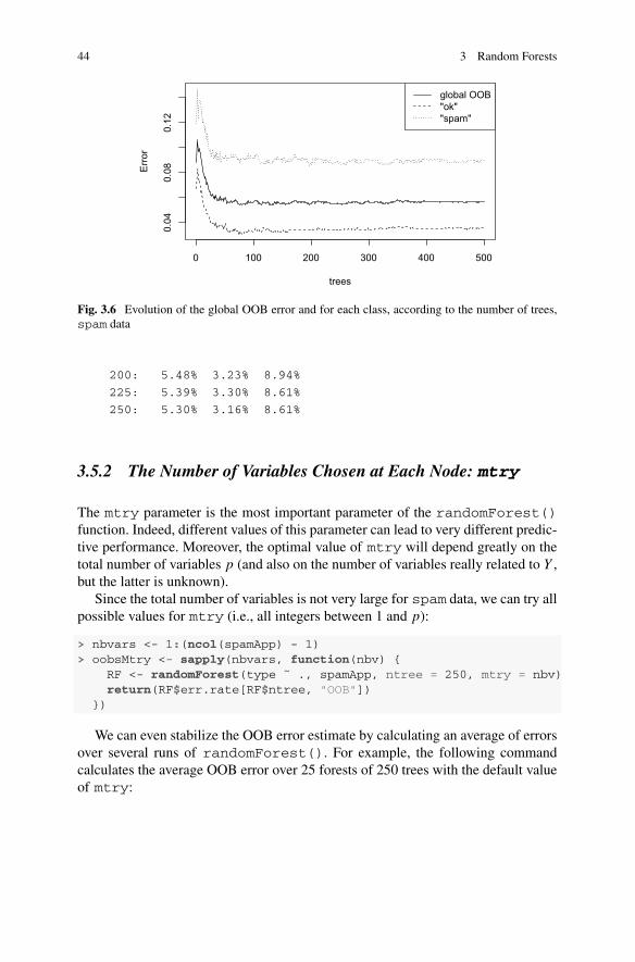
44 3 Random Forests
0 100 200 300 400 500
0.04
0.08
0.12
trees
Erro
r
global OOB"ok""spam"
Fig. 3.6 Evolution of the global OOB error and for each class, according to the number of trees,spam data
200: 5.48% 3.23% 8.94%
225: 5.39% 3.30% 8.61%
250: 5.30% 3.16% 8.61%
3.5.2 The Number of Variables Chosen at Each Node: mtry
The mtry parameter is the most important parameter of the randomForest()function. Indeed, different values of this parameter can lead to very different predic-tive performance. Moreover, the optimal value of mtry will depend greatly on thetotal number of variables p (and also on the number of variables really related to Y ,but the latter is unknown).
Since the total number of variables is not very large for spam data, we can try allpossible values for mtry (i.e., all integers between 1 and p):
> nbvars <- 1:(ncol(spamApp) - 1)> oobsMtry <- sapply(nbvars, function(nbv) {
RF <- randomForest(type ˜ ., spamApp, ntree = 250, mtry = nbv)return(RF$err.rate[RF$ntree, "OOB"])
})
We can even stabilize the OOB error estimate by calculating an average of errorsover several runs of randomForest(). For example, the following commandcalculates the average OOB error over 25 forests of 250 trees with the default valueof mtry:

3.5 Parameters Setting for Prediction 45
0 10 20 30 40 50
0.05
0.06
0.07
0.08
0.09
mtry
OO
B er
ror
25 RF1 RF
Fig. 3.7 OOB error as a function of mtry parameter value, spam data
> mean(replicate(n = 25, randomForest(type ˜ ., spamApp,ntree = 250)$err.rate[250, "OOB"]))
TheOOBerror evolution (Fig. 3.7) according tomtryvalue onour spam exampleis typical of standard (i.e., not high-dimensional) classification problems:
• If mtry is really too low, then the OOB error is relatively high (the extreme casewhere mtry is 1 is to choose the split variable completely at random at each node).
• When we increase mtry the error decreases quickly, until it reaches a minimum,then the error rises gradually.
In regression, we observe most of the time a decreasing behavior of the OOBerror as a function of mtry. The default value of the parameter is also higher inregression, equal to p/3 (instead of
√p in classification).
For a more detailed study of the mtry setting, we refer to Sect. 2 of Genuer et al.(2008).
Tree Diversity IllustrationTo conclude this section, let us illustrate the notion of tree diversity in a simple casewhere only two-leaf trees (also called stumps) are considered. Let us start by buildinga Bagging predictor made of 100 stumps:
> bagStump <- randomForest(type ˜ ., spamApp, ntree = 100,mtry = ncol(spamApp) - 1, maxnodes = 2)
Let us now look at which variables were used to split the root node of the 100trees:
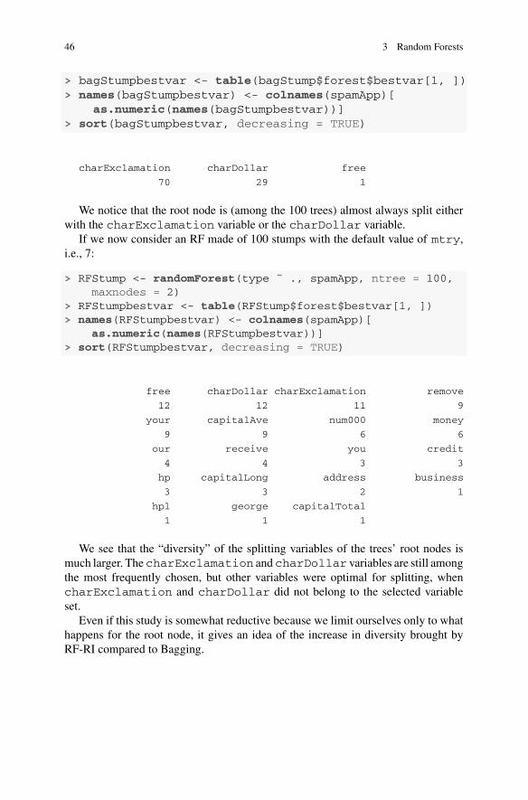
46 3 Random Forests
> bagStumpbestvar <- table(bagStump$forest$bestvar[1, ])> names(bagStumpbestvar) <- colnames(spamApp)[
as.numeric(names(bagStumpbestvar))]> sort(bagStumpbestvar, decreasing = TRUE)
charExclamation charDollar free
70 29 1
We notice that the root node is (among the 100 trees) almost always split eitherwith the charExclamation variable or the charDollar variable.
If we now consider an RF made of 100 stumps with the default value of mtry,i.e., 7:
> RFStump <- randomForest(type ˜ ., spamApp, ntree = 100,maxnodes = 2)
> RFStumpbestvar <- table(RFStump$forest$bestvar[1, ])> names(RFStumpbestvar) <- colnames(spamApp)[
as.numeric(names(RFStumpbestvar))]> sort(RFStumpbestvar, decreasing = TRUE)
free charDollar charExclamation remove
12 12 11 9
your capitalAve num000 money
9 9 6 6
our receive you credit
4 4 3 3
hp capitalLong address business
3 3 2 1
hpl george capitalTotal
1 1 1
We see that the “diversity” of the splitting variables of the trees’ root nodes ismuch larger. The charExclamation and charDollar variables are still amongthe most frequently chosen, but other variables were optimal for splitting, whencharExclamation and charDollar did not belong to the selected variableset.
Even if this study is somewhat reductive because we limit ourselves only to whathappens for the root node, it gives an idea of the increase in diversity brought byRF-RI compared to Bagging.

3.6 Examples 47
3.6 Examples
3.6.1 Predicting Ozone Concentration
For a presentation of this dataset, see Sect. 1.5.2.Let us load the randomForest package and Ozone data:
> library("randomForest")> data("Ozone", package = "mlbench")
Remark 3.7 It should be noted that, in this example, the standard theoretical frame-work that assumes observations as independent realizations from the same distribu-tion is inappropriate. Indeed, the serial dependence between two successive obser-vations is obvious and important since it carries both short-range dependence (theweather of the day is generally close to that of the next day) and long-range depen-dence because of the seasonal nature of both theweather and social life. Nevertheless,it appears that even in this context, random forests perform well.
Application of RF on this dataset can be done using the following command:
> OzRFDef <- randomForest(V4 ˜ ., Ozone, na.action = na.omit)
Note that the response variable, named V4, is located in the 4th column of the datatable. In addition, we must set the na.action parameter because we are dealingwith missing data. It should be noted that there are many of them (about 45% of theobservations contain at least one missing data) mainly because of V9. However, wewill simply omit them here.
Remark 3.8 The rfImpute() function of the randomForest package allows toimpute missing values using the proximities between complete observations. Prox-imity between two observations is the proportion of trees in which they appear inthe same terminal node of a given forest. The iterative imputation procedure can bededuced from this: the first forest is built using themedian imputation, the proximitiesare then calculated and new imputations are made by a weighted average accordingto the regression proximities or a weighted vote according to the classification prox-imities. A new forest is then built, giving new proximities and imputations, and theprocedure is iterated until the last imputation.
Let us display the results of this random forest:
> OzRFDef
Call:randomForest(formula = V4 ˜ ., data = Ozone, na.action = na.omit)
Type of random forest: regressionNumber of trees: 500

48 3 Random Forests
No. of variables tried at each split: 4
Mean of squared residuals: 21.20203% Var explained: 68.24
> plot(OzRFDef)
The plot of Fig. 3.8 illustrates both the gain brought by the aggregation of predic-tions provided by more and more trees (note, however, that compared to CART, theerror of a single tree is increased here because the trees are not pruned) and the factthat increasing the number of trees no longer provides anything essential (at least foraverage performance) from 50 or 100 trees and nothing at all from 200 trees.
More interestingly, it illustrates the absence of overfitting. Indeed, despite thesmall number of observations (less than 400 and even 200 without missing values)compared to the maximum number of trees in the forest (here 500), there is nooverfitting phenomenon: the error no longer decreases but does not increase either,it stabilizes.
In this example, the OOB error increases with mtry (Fig. 3.9), which is ratherunusual. In this case, it can be explained by the importance of the variables (seeSect. 4.5.2).
Remark 3.9 In this example, the response variable distribution is very asymmetricand large ozone concentration values are rare.Oneway to take this aspect into accountto some extent is to consider a stratified sampling, with respect to the concentrationof pollutants (V4), when selecting OOB samples, so as to preserve the distributionof the response variable in both bootstrap and OOB samples.
Bootstrap samples, and consequently OOB samples, can be stratified by creatinga factor, whose distribution will be used to stratify. Thus, we begin by dividing
0 100 200 300 400 500
2025
3035
4045
5055
OzRFDef
trees
Erro
r
Fig. 3.8 OOB error as a function of the number of trees, Ozone data

3.6 Examples 49
2 4 6 8 10 12
2021
2223
2425
26
mtry
OO
B er
ror
Fig. 3.9 OOB error as a function of mtry parameter value, Ozone data
the range of the response variable into 3 classes (values less than 10, between 10and 20, and greater than 20) according to which the stratification is performed. Thecommands below show how to proceed while eliminating the second temperaturevariable that has a lot of missing data.
> bins <- c(0, 10, 20, 40)> V4bin <- cut(Ozone$V4, bins, include.lowest = TRUE, right = FALSE)> OzoneBin <- data.frame(Ozone, V4bin)> OzRFDefStrat <- randomForest(V4 ˜ . - V9 - V4bin, OzoneBin,
strata = V4bin, sampsize = 200, na.action = na.omit)> OzRFDefStrat
Call:
randomForest(formula = V4 ˜ . - V9 - V4bin, data = OzoneBin,
strata = V4bin, sampsize = 200, na.action = na.omit)
Type of random forest: regression
Number of trees: 500
No. of variables tried at each split: 3
Mean of squared residuals: 22.22533
% Var explained: 66.7
The impact is not massive on this example, but in the case of ozone measuredin cities with more pronounced seasonal contrasts, this type of stratification can beuseful. In the following, we return to the basic version.

50 3 Random Forests
3.6.2 Analyzing Genomic Data
For a presentation of this dataset, see Sect. 1.5.3.Let us load the randomForest package and vac18 data:
> library(randomForest)> data("vac18", package = "mixOmics")
Then let us create an object geneExpr containing the gene expressions and anobject stimu containing the stimuli to be predicted:
> geneExpr <- vac18$genes> stimu <- vac18$stimulation
The training of a random forest is done with the following commands. Dealingwith high-dimensional data, we set the value from mtry to p/3.We recommend thisvalue of mtry in this case because the default value
√p (i.e., 31 in this example)
generally leads to consider too few informative variables in each node (Fig. 3.11).
> VacRFpsur3 <- randomForest(x = geneExpr, y = stimu,mtry = ncol(geneExpr)/3)
> VacRFpsur3> plot(VacRFpsur3)
Call:
randomForest(x = geneExpr, y = stimu, mtry = ncol(geneExpr)/3)
Type of random forest: classification
Number of trees: 500
No. of variables tried at each split: 333
OOB estimate of error rate: 35.71%
Confusion matrix:
LIPO5 GAG+ GAG- NS class.error
LIPO5 11 0 0 0 0.0000000
GAG+ 0 5 3 2 0.5000000
GAG- 0 4 2 4 0.8000000
NS 0 0 2 9 0.1818182
We see, thanks to the confusion matrix, giving in line the predicted class and incolumn the actual class, that the relatively high OOB error is largely due to the GAG-classwhich is predicted either inGAG+or inNS. This is because theGAG- stimulationis not only quite close to a “non-stimulation” but also has common features with theGAG+ stimulation.
According to Fig. 3.10, the OOB error stabilizes after about 100 trees have beenbuilt.
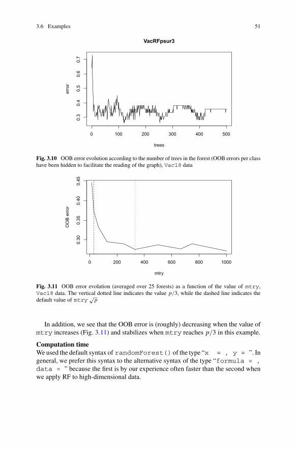
3.6 Examples 51
0 100 200 300 400 500
0.3
0.4
0.5
0.6
0.7
VacRFpsur3
trees
erro
r
Fig. 3.10 OOB error evolution according to the number of trees in the forest (OOB errors per classhave been hidden to facilitate the reading of the graph), Vac18 data
0 200 400 600 800 1000
0.30
0.35
0.40
0.45
mtry
OO
B er
ror
Fig. 3.11 OOB error evolution (averaged over 25 forests) as a function of the value of mtry,Vac18 data. The vertical dotted line indicates the value p/3, while the dashed line indicates thedefault value of mtry
√p
In addition, we see that the OOB error is (roughly) decreasing when the value ofmtry increases (Fig. 3.11) and stabilizes when mtry reaches p/3 in this example.
Computation timeWeused the default syntax of randomForest() of the type “x = , y = ”. Ingeneral, we prefer this syntax to the alternative syntax of the type “formula = ,data = ” because the first is by our experience often faster than the second whenwe apply RF to high-dimensional data.

52 3 Random Forests
Table 3.3 Comparison of execution times (medians on 25 runs) of the functionsrandomForest() and ranger(), Vac18 data
Function Type Time (in s)
randomForest() formula 0.705
randomForest() x, y 0.498
ranger() formula 0.402
ranger() x, y 0.392
Finally, still in the context of high-dimensional data, the use of the ranger packagecould give interesting results in terms of computation time (and according to our tests,the larger the dimension, the greater the gain).
A comparison of the computation times leads to the results of Table 3.3 (the timesdisplayed are median execution times over 25 runs).
Finally, it should be noted that the ranger() function allows parallel computingnatively. To do this, simply set the value of the num.threads parameter, whichby default is set to the number of cores available on the computer running the code(we set it to 1 to compare only non-parallelized commands).
3.6.3 Analyzing Dust Pollution
For a presentation of this dataset, see Sect. 1.5.4.Let us load the randomForest package and the JUS station data, included in the
VSURF package and create a dataframe jusComp containing no missing data:
> library(randomForest)> data("jus", package = "VSURF")> jusComp <- na.omit(jus)
Random forests and partial effectsRandom forests are a powerful and convenient tool to visualize, for each station, theeffects of variables on PM10 pollution and to identify important variables amongpollutants and weather variables.
> jusRF <- randomForest(PM10 ˜ ., data = jusComp)
To estimate the marginal effect of variable X j , we mimic the partial integrationof the forest (i.e., the estimated regression function), by using an empirical meanwhich approximates the expectation according to all variables except X j :
f j (x) = 1
n
n∑
i=1
h RF (x1i , . . . , xj−1i , x, x j+1
i , . . . , x pi ) .

3.6 Examples 53
0 50 100 150 200 250
2022
2426
2830
32
Marginal effect − NO
"NO"
Fig. 3.12 Marginal effect of NO variable on PM10 concentration, associated with a random foresttrained using station JUS data
The following command is used to compute the marginal effect of NO variable,at the JUS station (Fig. 3.12). In the same way, we can obtain marginal effects of allvariables at the JUS station (Fig. 3.13).
> partialPlot(jusRF, pred.data = jusComp, x.var = "NO",main = "Marginal effect - NO")
Remark 3.10 To go further on partial effects study, and especially if we are inter-ested in the effect of a pair of variables, we can use the forestFloor package (Wellinget al. 2016). This package provides 3D graphics and also adds color gradients usefulfor investigating interactions between explanatory variables.
For the other monitoring stations, the code (omitted here, as well as the graphics)is very similar as before. Indeed, only the name of the station changes and data for theother stations are also available in the VSURF package. By examining the marginaleffects of all variables on PM10 pollution for every monitoring station, the followingconclusions can be drawn.
First of all, we can state a general remark: intensities of partial effects of mete-orological variables are lower than those of pollutants. Indeed, consider a partialeffect of one pollutant. Realizations of concentrations of the other pollutants inte-grate weather factors and lead to coherent evolutions between pollutants. This is whywe will distinguish the effects of pollutants from those of the weather.
• Effects of pollutants. They are always increasing as expected, roughly linear inappearance, slightly convex or concave in shape depending on the pollutant andthe station.
• Rain effect. It is always decreasing since it reflects a cleaning effect.

54 3 Random Forests
NO NO2 SO2
PL.som T.moy DV.dom
VV.moy PA.moy
2024
2832
2024
28
2123
25
20.5
21.5
21.0
22.0
23.0
21.0
21.3
21.6
2226
20.5
21.5
21.0
22.5
24.0
GTrouen
0 50 100 150 200 250 0 20 40 60 80 0 10 20 30 40
0 10 20 30 40 −5 0 5 10 15 20 25 0 50 150 250 350
2 4 6 8 10 990 1010 1030 0 2 4 6 8
Fig. 3.13 Marginal effects of each variable on the PM10 concentration, from an RF trained onstation JUS
• Temperature effects. These are nonlinear effects: positive when it is cold or hot,zero or negative when the temperature is average.
• Effect of wind direction. Two situations must be distinguished:
– The one that is similar to JUS: GCM and AIL, where the effect of the winddirection shows an east/west axis.
– Or as for GUI, REP, HRI, where the effect of the direction shows an inhibitorynorth/south axis.
• Effect of wind speed. It is necessary to distinguish three situations according towhich the effect is inhibitory (for JUS and GUI) or decreasing (for GCM, REP,and HRI), what is expected, or even increasing for AIL. This is the only pointthat is, at first sight, surprising. It is explained by the absence of a local pollutionsource combined with a low level of pollution, which means that the main sourceis the import of pollution, hence the increasing effect of wind speed.
• Effect of relative humidity. Those effects are of very little importance and are veryrarely useful in the rest of the work. The weak min and max effects are different:increasing and decreasing, respectively.
• Effect of atmospheric pressure. It is still growing as expected.• Effect of temperature gradient. It is still growing as expected. The temperaturegradients of Le Havre and Rouen give very similar and equally important infor-mation.

3.6 Examples 55
ConclusionThe main conclusion is twofold:
• The effects of pollutants are always increasing, and are therefore markers of localpollution useful for dust modeling.
• For weather variables, we distinguish (by eliminating HR which is of low impor-tance)
– Those that have a rather unfavorable (decreasing) effect on pollution: PL andVV (for all stations except AIL).
– Those that have a favorable (increasing) effect: GT, PA, and VV (for AIL).– Those that have an unfavorable and then favorable effect: T (unfavorable if coldthen favorable when it is not cold), DV.
This study on marginal effects will be supplemented by the relative importanceof the variables (see Sect. 4.5.4).
Chapter 4Variable Importance
Abstract Here, the focus is on creating a hierarchy of input variables, based on aquantification of the importance of their effects on the response variable. Such anindex of importance provides a ranking of variables. Random forests offer an idealframework, as they do not make any assumptions regarding the underlying model.This chapter introduces permutation variable importance using random forests andillustrates its use on the spamdataset. The behavior of the variable importance index isfirst studied with regard to data-related aspects: the number of observations, numberof variables, and presence of groups of correlated variables. Then, its behavior withregard to random forest parameters is addressed. In the final section, the use ofvariable importance is first illustrated by simulation in regression, and then in threeexamples: predicting ozone concentration, analyzing genomic data, and determiningthe local level of dust pollution.
4.1 Notions of Importance
In this chapter, the focus is on constructing a hierarchy of explanatory variables basedon a quantification of the importance of their effects on the response variable. Suchan index of importance provides a ranking of variables, from the most importantto the least important. A general discussion on variable importance can be foundin Azen and Budescu (2003). This notion has been mainly studied in the contextof linear models, as highlighted by Grömping (2015)’s review or Wallard (2015)’sPhD thesis. From this standpoint, random forests offer an ideal framework, as theyare much more general and, as previously mentioned, do not make any assumptionsregarding the underlying model. They combine a nonparametric method, which doesnot specify a particular type of the relationship between Y and X , with resamplingto provide an efficient and convenient definition of such indices.
In this context, one of the most widely used measures of the importance of agiven variable is the average (among trees in a forest) increase in the error made by
© Springer Nature Switzerland AG 2020R. Genuer and J.-M. Poggi, Random Forests with R, Use R!,https://doi.org/10.1007/978-3-030-56485-8_4
57
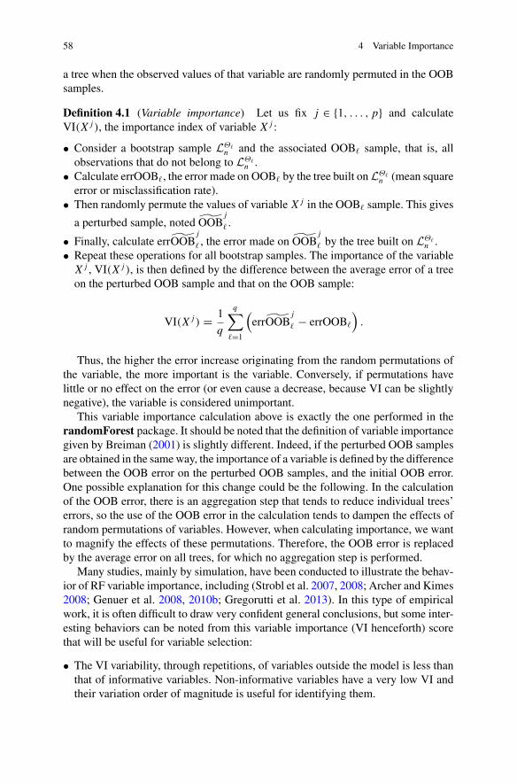
58 4 Variable Importance
a tree when the observed values of that variable are randomly permuted in the OOBsamples.
Definition 4.1 (Variable importance) Let us fix j ∈ {1, . . . , p} and calculateVI(X j ), the importance index of variable X j :
• Consider a bootstrap sample LΘ�n and the associated OOB� sample, that is, all
observations that do not belong to L�n .
• Calculate errOOB�, the error made on OOB� by the tree built onLΘ�n (mean square
error or misclassification rate).• Then randomly permute the values of variable X j in the OOB� sample. This gives
a perturbed sample, noted ˜OOBj
� .
• Finally, calculate err˜OOBj
� , the error made on ˜OOBj
� by the tree built on L�n .
• Repeat these operations for all bootstrap samples. The importance of the variableX j , VI(X j ), is then defined by the difference between the average error of a treeon the perturbed OOB sample and that on the OOB sample:
VI(X j ) = 1
q
q∑
�=1
(err˜OOB
j
� − errOOB�
).
Thus, the higher the error increase originating from the random permutations ofthe variable, the more important is the variable. Conversely, if permutations havelittle or no effect on the error (or even cause a decrease, because VI can be slightlynegative), the variable is considered unimportant.
This variable importance calculation above is exactly the one performed in therandomForest package. It should be noted that the definition of variable importancegiven by Breiman (2001) is slightly different. Indeed, if the perturbed OOB samplesare obtained in the sameway, the importance of a variable is defined by the differencebetween the OOB error on the perturbed OOB samples, and the initial OOB error.One possible explanation for this change could be the following. In the calculationof the OOB error, there is an aggregation step that tends to reduce individual trees’errors, so the use of the OOB error in the calculation tends to dampen the effects ofrandom permutations of variables. However, when calculating importance, we wantto magnify the effects of these permutations. Therefore, the OOB error is replacedby the average error on all trees, for which no aggregation step is performed.
Many studies, mainly by simulation, have been conducted to illustrate the behav-ior of RF variable importance, including (Strobl et al. 2007, 2008; Archer and Kimes2008; Genuer et al. 2008, 2010b; Gregorutti et al. 2013). In this type of empiricalwork, it is often difficult to draw very confident general conclusions, but some inter-esting behaviors can be noted from this variable importance (VI henceforth) scorethat will be useful for variable selection:
• The VI variability, through repetitions, of variables outside the model is less thanthat of informative variables. Non-informative variables have a very low VI andtheir variation order of magnitude is useful for identifying them.

4.1 Notions of Importance 59
• In the presence of a group of highly correlated variables, masking effects appearbut remain limited except when the number of variables in the group is dominantcompared to other informative variables.
• A stable evaluation of these VI requires, on the one hand, large forests (with ahigh number of trees) and, on the other hand, some repetitions of such forests tobe able to quantify their variability.
Wewill now focus on RF prediction performance by estimating the generalizationerror by out-of-bag error (OOB) and quantifying the permutation-based variableimportance that are the main ingredients of our variable selection strategy, presentedin Chap. 5.
To obtain the calculation of the permutation-based VI, it is necessary to add theoption importance = TRUE in the randomForest() function:
> RFDefImp <- randomForest(type ˜ ., data = spamApp,importance = TRUE)
> varImpPlot(RFDefImp, type = 1, scale = FALSE,n.var = ncol(spamApp) - 1, cex = 0.8,main = "Variable importance")
We can see in Fig. 4.1 a quantification of VI for spam data. It is both enlighteningand easily interpretable. It makes it possible to identify very clearly a first group ofvariables: capitalLong, remove, hp, charExclamation, capitalAve,capitalTotal,free, andcharDollar then, less clearly, a group of 8 variableswhich contains useful variables not only likegeorgebut alsoyouror number000whose presence is less intuitive.
Itmay be noted that themost important variable (capitalLong) does not appearin any of the splits in the optimal tree, which proves that a variable that never comesout in the local minimization of heterogeneity can nevertheless be important becauseit is well correlated with all informative variables.
Remark 4.1 The varImpPlot() function of randomForest package allows todirectly plot the importance of the variables classified in decreasing order of impor-tance. However, we emphasize that we indicate type = 1 because we only wantto plot the permutation-based VI,1 and scale = FALSE to get the raw impor-tance, and not the normalized importance for which the average of the trees’ errorsis divided by the standard deviation of these errors.
In Gregorutti et al. (2015), the notion of permutation-basedVI is directly extendedto a group of variables. To do this, it suffices to permute, in theOOB samples involvedin the VI definition (see Definition 4.1), not only one variable but jointly all thevariables of the same group. For functional additive models, the theoretical resultsof Gregorutti et al. (2013) are extended. Then a strategy for selecting variables in amultivariate functional data framework is derived by selecting groups of variables
1The option type = 2 allows obtaining the MDI importance, defined in the next paragraph.

60 4 Variable Importance
partstablenum3dreportdirectnum857datanum415makeconferencecscharHashprojectoriginalpeopleaddressestelnetpmlabcharSquarebrackettechnologycreditcharSemicolonorderaddressfontemailoverlabsreceivenum85charRoundbracketallmailmeetingwillnum650businessreinternetnum1999youmoneyedunum000ourhplyourgeorgefreecapitalAvehpcapitalTotalcharDollarcapitalLongremovecharExclamation
0.00 0.01 0.02 0.03
Variable importance
MeanDecreaseAccuracy
Fig. 4.1 Importance of variables ranked in descending order for spam data
made of wavelet coefficient sets, representing the different functional variables, andusing a Recursive Feature Elimination (RFE) strategy. These tools are available inthe RFgroove package (Gregorutti 2016).
Finally, the very recent work of Ramosaj and Pauly (2019) shows that, at least inthe case where input variables are independent, the permutation-based VI is asymp-totically unbiased.

4.1 Notions of Importance 61
MDI ImportanceIt should be noted that there is another VI index based on the Mean Decrease Impu-rity (MDI) and inspired by the variable importance defined in CART method (seeSect. 2.5.3). It is defined as follows (Breiman 2001): for a given variable, its MDI isthe sum of the impurity decreases for all nodes where the variable is used to split,weighted by the proportion of individuals in the node, on average on all trees in theforest. Although its use seems less frequent, it has given rise to theoretical results(Louppe et al. 2013) and finds interesting practical applications despite real limita-tions. In particular, it is highly dependent on forest parameters, biased for non-prunedtrees and finally the theoretical results only cover binary categorical variables.
4.2 Variable Importance Behavior
We illustrate the behavior of the permutation-based variable importance on a simu-lated dataset, called toys. Introduced byWeston et al. (2003), it is a binary classifica-tion problem (Y ∈ {−1, 1}), with 6 “true” variables (related to Y ) and noise variables(independent of Y ). For the latter, we will speak indifferently of variables that areout of model or not informative.
The 6 true variables are divided into two independent groups: variables V1, V2,and V3 on the one hand and variables V4, V5, and V6 on the other hand.
Definition 4.2 (Toys model) The simulation model is defined using the distributionof input variables X j conditionally to Y = y as follows:
• For 70%of theobservations: X j ∼ N (y × j, 1) for j = 1, 2, 3and X j ∼ N (0, 1)for j = 4, 5, 6.
• For the remaining 30% of observations: X j ∼ N (0, 1) for j = 1, 2, 3 and X j ∼N (y × ( j − 3), 1) for j = 4, 5, 6.
The additional noise variables, when p > 6, are generated independently of Y :X j ∼ N (0.1) for j = 7, . . . , p.
Once simulated, the input variables are all standardized.
Figure 4.2 gives the histograms of the first 9 input variables for a simulation of1,000 observations based on toys model. The definition of the toys model as well asthe distribution of the input variables highlight the fact that the variables of the samegroup are sorted from the least related to Y to the most related to Y .
4.2.1 Behavior According to n and p
Starting from a classical situation with n = 500 and p = 6, illustrating a very goodresult of VI computation, we show in Fig. 4.3 the behavior of VI when increasingthe number of input variables and also when decreasing the number of observations.

62 4 Variable Importance
V1
−4 −2 0 1 2 3 −4 −2 0 1 2 3 −4 −2 0 1 2 3
−4 −2 0 1 2 3 −4 −2 0 1 2 3 −4 −2 0 1 2 3
−4 −2 0 1 2 3 −4 −2 0 1 2 3 −4 −2 0 1 2 3
V2 V3
V4 V5 V6
V7 V8 V9
0.0
0.1
0.2
0.3
0.4
0.5
0.0
0.1
0.2
0.3
0.4
0.5
0.0
0.1
0.2
0.3
0.4
0.5
0.0
0.1
0.2
0.3
0.4
0.5
0.0
0.1
0.2
0.3
0.4
0.5
0.0
0.1
0.2
0.3
0.4
0.5
0.0
0.1
0.2
0.3
0.4
0.5
0.0
0.1
0.2
0.3
0.4
0.5
0.0
0.1
0.2
0.3
0.4
0.5
Fig. 4.2 Histogramsof thefirst 9 input variables of toysmodel for a simulation of 1,000observations
The graphs in the first row of Fig. 4.3 illustrate that in the case of a high numberof observations, the importance of the variables behaves well (in the sense that V1 toV6 are the most important) even when the dimension increases. Indeed, even if theimportance of the variables in the model decreases, they remain much higher thanthe importance of variables outside the model.
In the second row, we see that even in cases where p > n, the overall behav-ior remains satisfactory, even if importance of variable V4 no longer differs fromout-of-model variables when p = 200 or p = 500. However, this variable is quiteuninformative in this simulation model.
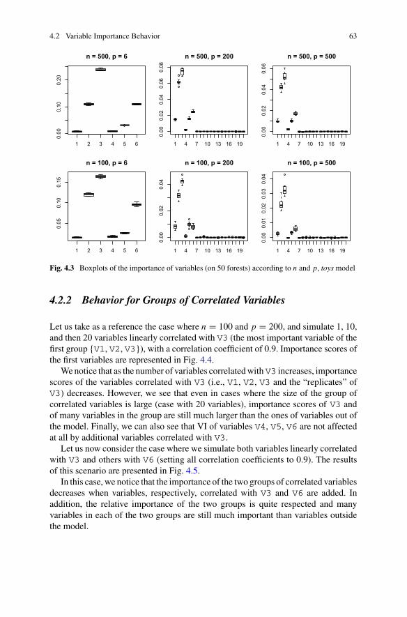
4.2 Variable Importance Behavior 63
n = 500, p = 6
1 4 7 10 13 16 19 1 4 7 10 13 16 19
1 4 7 10 13 16 19 1 4 7 10 13 16 19
n = 500, p = 200 n = 500, p = 500
1 2 3 4 5 6
1 2 3 4 5 6
n = 100, p = 6 n = 100, p = 200 n = 100, p = 500
0.00
0.10
0.20
0.00
0.02
0.04
0.06
0.08
0.00
0.02
0.04
0.06
0.05
0.10
0.15
0.00
0.02
0.04
0.00
0.01
0.02
0.03
0.04
Fig. 4.3 Boxplots of the importance of variables (on 50 forests) according to n and p, toys model
4.2.2 Behavior for Groups of Correlated Variables
Let us take as a reference the case where n = 100 and p = 200, and simulate 1, 10,and then 20 variables linearly correlated with V3 (the most important variable of thefirst group {V1, V2, V3}), with a correlation coefficient of 0.9. Importance scores ofthe first variables are represented in Fig. 4.4.
We notice that as the number of variables correlatedwith V3 increases, importancescores of the variables correlated with V3 (i.e., V1, V2, V3 and the “replicates” ofV3) decreases. However, we see that even in cases where the size of the group ofcorrelated variables is large (case with 20 variables), importance scores of V3 andof many variables in the group are still much larger than the ones of variables out ofthe model. Finally, we can also see that VI of variables V4, V5, V6 are not affectedat all by additional variables correlated with V3.
Let us now consider the case where we simulate both variables linearly correlatedwith V3 and others with V6 (setting all correlation coefficients to 0.9). The resultsof this scenario are presented in Fig. 4.5.
In this case, we notice that the importance of the two groups of correlated variablesdecreases when variables, respectively, correlated with V3 and V6 are added. Inaddition, the relative importance of the two groups is quite respected and manyvariables in each of the two groups are still much important than variables outsidethe model.
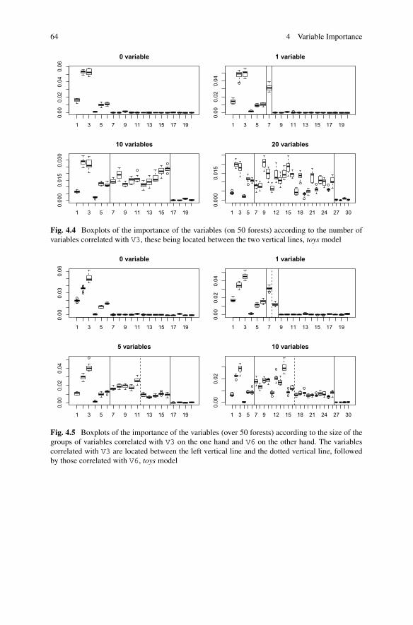
64 4 Variable Importance
0 variable 1 variable
10 variables 20 variables
0.00
0.02
0.04
0.06
0.00
0.02
0.04
0.00
00.
015
0.03
0
0.00
00.
015
1 3 5 7 9 11 13 15 17 19 1 3 5 7 9 11 13 15 17 19
1 3 5 7 9 11 13 15 17 19 1 3 5 7 9 12 15 18 21 24 27 30
Fig. 4.4 Boxplots of the importance of the variables (on 50 forests) according to the number ofvariables correlated with V3, these being located between the two vertical lines, toys model
0 variable 1 variable
5 variables
0.00
0.03
0.06
0.00
0.02
0.04
0.00
0.02
0.04
0.00
0.02
10 variables
1 3 5 7 9 11 13 15 17 19 1 3 5 7 9 11 13 15 17 19
1 3 5 7 9 11 13 15 17 19 1 3 5 7 9 12 15 18 21 24 27 30
Fig. 4.5 Boxplots of the importance of the variables (over 50 forests) according to the size of thegroups of variables correlated with V3 on the one hand and V6 on the other hand. The variablescorrelated with V3 are located between the left vertical line and the dotted vertical line, followedby those correlated with V6, toys model

4.3 Tree Diversity and Variables Importance 65
4.3 Tree Diversity and Variables Importance
Let us go back to the simple case where we consider only stumps (two-leaf trees). InSect. 3.5.2, we highlight the effect of mtry on the variables used in the root node.
Let us now focus on the effect of this tree diversity on variable importance, byagain building a Bagging predictor only made of stumps on spam data, but nowwithVI computation:
> bagStumpImp <- randomForest(type ˜ ., spamApp,mtry = ncol(spamApp) - 1, maxnodes = 2, importance = TRUE)
> varImpPlot(bagStumpImp, type = 1, scale = FALSE, n.var = 20,cex = 0.8, main = "Variable importance")
In Fig. 4.6, we observe that almost all the variables are of no importance, and weonly detect variables charExclamation and charDollar, which is consistentwith the fact that only these two variables are actually used to split the root node.
Now let us compare it to an RF only made of stumps, built with the default valueof mtry (equal to 7 here):
> RFStumpImp <- randomForest(type ˜ ., spamApp, maxnodes = 2,importance = TRUE)
> varImpPlot(RFStumpImp, type = 1, scale = FALSE, n.var = 20,cex = 0.8, main = "Variable importance")
emailbusinessfreeaddressesreportpeoplewillreceivemailorderinternetoverournum3dalladdressmakeremovecharExclamationcharDollar
0.00 0.05 0.10 0.15 0.20
Variable importance
MeanDecreaseAccuracy
Fig. 4.6 Importance of the 20 most important variables for a Bagging of stumps, spam data

66 4 Variable Importance
addressemailmailreceiveinternetbusinessallhpyoucapitalTotalourcapitalLongnum000capitalAvemoneyfreeremoveyourcharDollarcharExclamation
0.000 0.005 0.010 0.015 0.020 0.025
Variable importance
MeanDecreaseAccuracy
Fig. 4.7 Importance of the 20 most important variables for an RF of stumps with the default valueof mtry (equal to 7), spam data
We observe (Fig. 4.7) that many more variables are of strictly positive importance(the randomization at the variable level actually changes the subset of variableschosen at each node to participate in the split). Moreover, the variables that emergewith the greatest importance are almost the same as those from an RF with maximaltrees, ignoring the order. Thus, even with trees that are clearly not complex enough,RF can retrieve the interesting information contained in the variables.
4.4 Influence of Parameters on Variable Importance
If the only goal is to achieve good predictive performance with RF, we recommendadjusting the RF parameters based on the OOB error. However, when we also wishto have information on the variables, or even to select variables, we must try to adjustthe RF parameters by looking at their impact on VI.
We illustrate the behavior of VI as a function of parameters in the toys simulationmodel. We start from the framework where n = 100 and p = 200 and represent inFig. 4.8 the VI obtained by varying the number of trees ntree (on rows) and themtry parameter (on columns).
Increasing the number of trees has the effect of stabilizing the VI, and the defaultvalue 500 seems large enough in this example. On the other hand, when the valueof mtry increases, we notice that the importance of the most influential variablesof the model increases, with a very large increase when going from 14 (which is

4.4 Influence of Parameters on Variable Importance 67
1 4 7 10 13 16 19 1 4 7 10 13 16 19 1 4 7 10 13 16 19
1 4 7 10 13 16 19 1 4 7 10 13 16 19 1 4 7 10 13 16 19
1 4 7 10 13 16 19 1 4 7 10 13 16 19 1 4 7 10 13 16 19
ntree = 100, mtry = 14 ntree = 100, mtry = 100 ntree = 100, mtry = 200
ntree = 500, mtry = 14 ntree = 500, mtry = 100 ntree = 500, mtry = 200
ntree = 2000, mtry = 14 ntree = 2000, mtry = 100
0.00
0.02
0.04
0.06
0.08
0.00
0.05
0.10
0.15
0.20
0.00
0.10
0.20
0.30
0.00
0.02
0.04
0.06
0.00
0.05
0.10
0.15
0.20
0.00
0.10
0.20
0.30
0.00
0.02
0.04
0.06
0.00
0.05
0.10
0.15
0.20
0.00
0.10
0.20
0.30
ntree = 2000, mtry = 200
Fig. 4.8 Boxplot of the importance of the variables (on 50 forests) according to ntree and mtry,toys model
the default value of randomForest()) to 100. Finally, we also see a stabilizationeffect of VI when the value of mtry increases.
Thus, in a very parsimonious case such as the one studied here (6 variables relatedtoY among200), it seems necessary to increase the value of mtry in order to stabilizeimportance of model variables and to help highlighting themost influential variables.

68 4 Variable Importance
4.5 Examples
4.5.1 An Illustration by Simulation in Regression
We use a simple example in regression, to illustrate the use of variable importance inthis context, as well as the use of partial effects (defined in Sect. 3.6.3). In this classicexample introduced in Friedman (1991) and accessible via the mlbench package,observations are generated by the following model:
Y = 10 sin(π X1 X2) + 20(X3 − 0.5)2 + 10 X4 + 5 X5 + ε
and in which there are 10 input variables assumed independent and with the sameuniform distribution on [0, 1]. Thus, only 5 of them are actually used to generate theoutputs and, moreover, it is assumed that ε ∼ N (0, 1).
Let us simulate 500 observations using the model and build an RF with VI com-putation:
> library(mlbench)> fried1Simu <- mlbench.friedman1(n = 500)> fried1Data <- data.frame(fried1Simu$x, y = fried1Simu$y)> fried1RFimp <- randomForest(y ˜ ., fried1Data, importance = TRUE)> varImpPlot(fried1RFimp, type = 1, scale = FALSE,
main = "Variable importance")
Variable importance (Fig. 4.9) clearly identifies the 5 variables in the model thatactually contribute to response computation and discards the non-informative vari-ables.
X6X9X8X7X10X3X5X1X2X4
0 2 4 6 8 10 12
Variable importance
%IncMSE
Fig. 4.9 Importance of variables, simulated data in regression
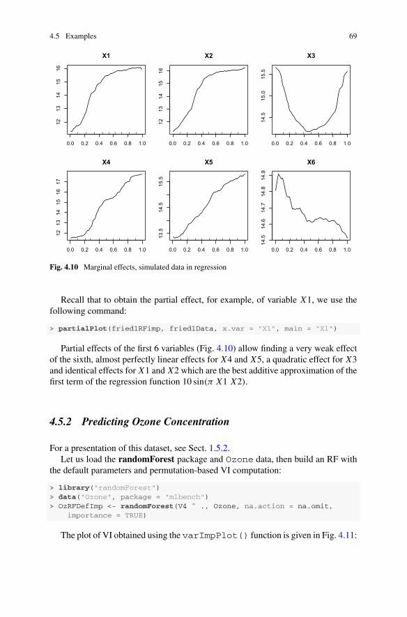
4.5 Examples 69
0.0 0.2 0.4 0.6 0.8 1.0 0.0 0.2 0.4 0.6 0.8 1.0 0.0 0.2 0.4 0.6 0.8 1.0
0.0 0.2 0.4 0.6 0.8 1.0 0.0 0.2 0.4 0.6 0.8 1.0 0.0 0.2 0.4 0.6 0.8 1.0
X1 X2 X3
X4 X5
1213
1415
16
1213
1415
16
14.5
15.0
15.5
1213
1415
1617
13.5
14.5
15.5
14.5
14.6
14.7
14.8
14.9
X6
Fig. 4.10 Marginal effects, simulated data in regression
Recall that to obtain the partial effect, for example, of variable X1, we use thefollowing command:
> partialPlot(fried1RFimp, fried1Data, x.var = "X1", main = "X1")
Partial effects of the first 6 variables (Fig. 4.10) allow finding a very weak effectof the sixth, almost perfectly linear effects for X4 and X5, a quadratic effect for X3and identical effects for X1 and X2 which are the best additive approximation of thefirst term of the regression function 10 sin(π X1 X2).
4.5.2 Predicting Ozone Concentration
For a presentation of this dataset, see Sect. 1.5.2.Let us load the randomForest package and Ozone data, then build an RF with
the default parameters and permutation-based VI computation:
> library("randomForest")> data("Ozone", package = "mlbench")> OzRFDefImp <- randomForest(V4 ˜ ., Ozone, na.action = na.omit,
importance = TRUE)
The plot of VI obtained using the varImpPlot() function is given in Fig. 4.11:

70 4 Variable Importance
V2V3V6V13V7V10V11V5V1V12V8V9
0 5 10 15 20
Variable importance
%IncMSE
Fig. 4.11 Importance of variables, obtained with a default RF, Ozone data
> varImpPlot(OzRFDefImp, type = 1, scale = FALSE,main = "Variable importance")
This dataset has already been the subject of many studies and, even if they arereal data, it is possible to know a priori which variables are supposed to be the mostimportant and, on the other hand, which are the main sources of nonlinearity.
As noted in previous studies, three groups of very easily interpretable variablescan be identified, ranging from the most important to the least important:
• The first group contains the two temperatures (V8 and V9) and the inversionbase temperature (V12), known to be the best ozone predictors, and the monthnumber (V1), which is an important predictor since ozone concentration has astrong seasonal component.
• The second group of significantly less important meteorological variables includespressure height (V5), humidity (V7), basic inversion height (V10), pressure gra-dient (V11), and visibility (V13).
• Finally, the last group contains three irrelevant variables: the day of themonth (V2),the day of the week (V3) as expected, and more surprisingly the wind speed (V6).The latter is a classic fact: the wind only enters the model when ozone pollutionoccurs, otherwise wind and pollution are weakly correlated and since most of thetime pollution levels are moderate, this explains the low overall importance of thewind.
Let us go back to V2which appeared high in the default tree obtained in Fig. 2.10.Variable importance thus shows a very satisfactory behavior by eliminating the effectsof the selection bias of this variable in the splits.
Finally, as we noticed in Sect. 3.6.1, in this example, the OOB error increaseswith mtry, which is unusual. This can be explained by studying the behavior of the
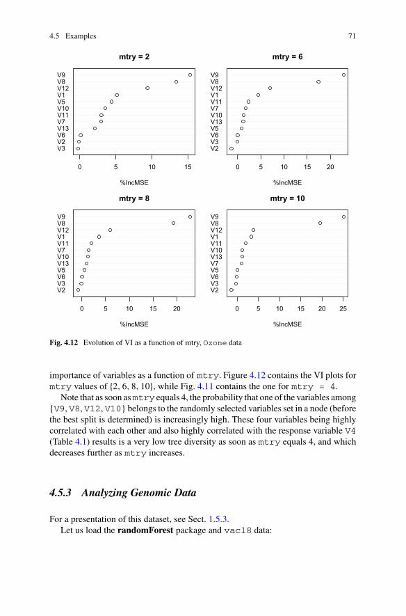
4.5 Examples 71
V3V2V6V13V7V11V10V5V1V12V8V9
mtry = 2
%IncMSE
V2V3V6V5V13V10V7V11V1V12V8V9
mtry = 6
%IncMSE
V2V3V6V5V13V10V7V11V1V12V8V9
mtry = 8
%IncMSE
V2V3V6V5V7V13V10V11V1V12V8V9
0 5 10 15 0 5 10 15 20
0 5 10 15 20 0 5 10 15 20 25
mtry = 10
%IncMSE
Fig. 4.12 Evolution of VI as a function of mtry, Ozone data
importance of variables as a function of mtry. Figure 4.12 contains the VI plots formtry values of {2, 6, 8, 10}, while Fig. 4.11 contains the one for mtry = 4.
Note that as soon asmtry equals 4, the probability that one of the variables among{V9, V8, V12, V10} belongs to the randomly selected variables set in a node (beforethe best split is determined) is increasingly high. These four variables being highlycorrelated with each other and also highly correlated with the response variable V4(Table 4.1) results is a very low tree diversity as soon as mtry equals 4, and whichdecreases further as mtry increases.
4.5.3 Analyzing Genomic Data
For a presentation of this dataset, see Sect. 1.5.3.Let us load the randomForest package and vac18 data:

72 4 Variable Importance
Table 4.1 Variable correlation matrix V4, V8, V9, V10, and V12, Ozone data
V4 V8 V9 V10 V12
V4 1.00 0.76 0.75 −0.54 0.70
V8 0.76 1.00 0.91 −0.51 0.84
V9 0.75 0.91 1.00 −0.59 0.93
V10 −0.54 −0.51 −0.59 1.00 −0.79
V12 0.70 0.84 0.93 −0.79 1.00
> library(randomForest)> data("vac18", package = "mixOmics")
Then let us create an object geneExpr containing the gene expressions and anobject stimu containing the stimuli to be predicted:
> geneExpr <- vac18$genes> stimu <- vac18$stimulation
An RF, computing permutation-based VI and with the mtry parameter set top/3 (as mentioned in Sect. 3.6.2, the default value, equal to 31, is too low for thishigh-dimensional dataset) is obtained as follows:
> vacRFDefImp <- randomForest(x = geneExpr, y = stimu,mtry = ncol(geneExpr)/3, importance = TRUE)
The varImpPlot() function returns by default the importance of the variablesfor the 30 most important variables (see Fig. 4.13):
> varImpPlot(vacRFDefImp, type = 1, scale = FALSE, cex = 0.8)
A plot of VI of all variables (representation used in Chap. 5) can be obtained withthe following commands:
> vacImp <- vacRFDefImp$importance[, nlevels(stimu) + 1]> plot(sort(vacImp, decreasing = TRUE), type = "l",
xlab = "Variables", ylab = "Variable importance")
The shape of the curve plotted in Fig. 4.14 is quite standard in high dimension andhighlights a very strong sparsity for Vac18 data. Indeed, we see that only a smallnumber of variables have a significantly positive VI score.

4.5 Examples 73
ILMN_1785158ILMN_1672446ILMN_1673023ILMN_1768812ILMN_1681644ILMN_1796685ILMN_1663032ILMN_2406335ILMN_1658145ILMN_1754547ILMN_2067444ILMN_2261784ILMN_1693221ILMN_1713156ILMN_1854015ILMN_3309644ILMN_1694608ILMN_1745271ILMN_1782685ILMN_2188204ILMN_1695421ILMN_3252733ILMN_1736939ILMN_2102693ILMN_2136089ILMN_2124802ILMN_1686664ILMN_1691156ILMN_1775170ILMN_1718766
0.00 0.01 0.02 0.03
vacRFDefImp
MeanDecreaseAccuracy
Fig. 4.13 Importance of the 30 most important variables sorted in descending order, Vac18 data
0 200 400 600 800 1000
0.00
0.01
0.02
0.03
Variables
Varia
ble
impo
rtanc
e
Fig. 4.14 Importance of all variables sorted in descending order of importance, Vac18 data

74 4 Variable Importance
4.5.4 Air Pollution by Dust: What Is the Local Contribution?
We continue here the example of dust pollution in the network of the Haute-Normandie region (Sect. 3.6.3), this time taking inspiration from the work of Bobbiaet al. (2011). We do not provide details on the R code used in this part, but prefer toshow another example of the possible use of variable importance.
In France, several regional plans have been defined to reduce pollution. In thiscontext, determining the local contribution in relation to the background contributionof a specific pollution is necessary. This makes it possible to assess the proportionof pollution on which it is possible to act and can help to adapt the regional plan. Anassessment of the local contribution can be carried out using deterministicmodels thatprovide a pollution map of the entire country at a regional scale. They are not relatedto pollution measurements at monitoring sites but depend on imprecise and difficultto obtain emissions inventory. The large uncertainties that result from this thereforelead to the use of statistical tools rather than a purely deterministic approach. Anexample of such an approach has recently been conducted in the Haute-Normandieregion to quantify local and background contributions specifically to dust pollution.
In the first step, the marginal effects were classified according to the character-istics of the monitoring stations: some are close to traffic, others measure urban orindustrial background pollution, and the last is located in a rural area. Local pollutionis thus characterized by conventional pollutants, including nitrogen oxides for urbanpollution and sulfur dioxide for industrial use. It should be recalled that three groupsof meteorological variables have been structured in the following way-those withan adverse effect on pollution: PL and VV (for all stations except AIL); a positiveeffect: GT, PA, and VV (for AIL); and a non-monotonic effect: T, DV.
Then, for each of the six monitoring stations, the individual VI is computed usingan RF model containing a large number of variables. To define the importance ofa group of variables, we propose to adopt the following rule: if the variables of thegroup are redundant (either well correlated or, more weakly, with similar “effects onPM10 concentrations”) then the importance of the group is defined by the maximumindividual VI in this group. In this way, groups of variables can be directly compared.The results are summarized in Table 4.2.
The importance of the three groups of weather variables is almost equal to 20, withthe exception of PA for GUI which reaches 32. On the other hand, the importance ofpollutants (by restricting ourselves to the largest importance) fluctuates much more:from 28 to 49 if we exclude AIL since no measurement of pollutants were madethere.
The two traffic stations (GUI and REP) give close values for the NO2 importance(41 and 45). The two urban stations (JUS and HRI), on the other hand, have differentimportance for SO2: 28 and 49, respectively. For the industrial station (GCM), theimportance of the pollutant (SO2) is 39, which is intermediate.
The idea is to use the pollution from the AIL station (noted as PM10_AIL) as ameasure of diffuse pollution at the regional level. It is supposed to capture phenomenaon a more or less large scale (regional or more) and not be affected by significant

4.5 Examples 75
Table 4.2 Importance of variables, through stations, for pollutants and meteorological variables bygroup, where def means that the effect is unfavorable (increasing), fav that it is favorable (decreas-ing), and def-fav for non-monotonic effects on PM10 pollution
Pollutants Meteo def Meteo fav Meteo def-fav
GCM Rouen 39 (SO2) 23 (PL) 20 (GT) 21 (T)
JUS Rouen 28 (NO2) 19 (PL) 21 (GT) 19 (DV)
22 (SO2)
GUI Rouen 41 (NO2) 18 (PL) 32 (PA) 19 (T)
18 (SO2)
AIL Dieppe 15 (PL) 23 (PA) 21 (DV)
REP Le Havre 45 (NO2) 20 (VV) 24 (GT) 19 (T)
31 (SO2)
HRI Le Havre 22 (NO2) 16 (VV) 18 (GT) 22 (T)
49 (SO2)
Table 4.3 Importance scores of variables, through stations, for pollutants and meteorological vari-ables by group, by adding PM10_AIL in the RF model
Pollutants Meteo def Meteo fav Meteo def-fav PM10_AIL
GCM 33 (SO2) 23 (PL) 17 (GT) 16 (DV) 68
JUS 31 (NO) 19 (PL) 16 (GT) 13 (DV) 78
18 (SO2)
GUI 40 (NO2) 18 (PL) 26 (PA) 20 (T) 64
17 (SO2)
REP 28 (SO2) 18 (VV) 19 (GT) 12 (T) 81
44 (NO2)
HRI 41 (SO2) 12 (VV) 11 (GT) 13 (T) 86
14 (NO)
local production. This is supported by examining the concentration distributions at allstations for days when PM10_AIL exceeds 30 (33 days are concerned): the medianis around 40 and the first quartile around 33.
The computation of the importance of variable PM10_AIL in previous modelswhen completed by the introduction of this new variable leads to the results recordedin Table 4.3:
• Its importance is in the order of 64 to 86, which is considerable.• The importance of pollutants fluctuates a little bit, and this is for all stations.• The importance of weather variables decreases significantly.
These elements are consistent with the idea that PM10 concentrations at AILreflect diffuse pollution in the sense that it does not perturb the importance of localmarkers while it affects the importance of weather variables.

76 4 Variable Importance
Table 4.4 Importance of variables, through stations, for pollutants and after replacing meteorolog-ical variables by PM10_AIL in forest variables
Main pollutant Other pollutants PM10_AIL
GCM 73 (SO2) 98
JUS 35 (NO) 26, 22 (NO2, SO2) 89
GUI 42 (NO2) 31, 20 (NO, SO2) 77
REP 42 (SO2) 41, 36 (NO2, NO) 78
HRI 50 (SO2) 21, 19 (NO, NO2) 81
For each of the other five stations, an RF is then trained with VI computationbased on available pollutants and PM10 concentrations at AIL only. This eliminatesall weather variables. The results of the importance are gathered in Table 4.4.
All partial effects are generally increasing and weakly nonlinear (except some-times for extreme SO2 levels). The interpretation is as follows: by introducing thisvariable, which seems to capture a kind of diffuse pollution by dust, the model isalmost linearized.
In conclusion, thanks to such a method, it has been possible to consider that inthe Haute-Normandie region, the importance of the local share of dust pollution,which can be controlled by regulatory measures, does not generally exceed that oflarge-scale pollution.

Chapter 5Variable Selection
Abstract This chapter is dedicated to variable selection using random forests: anautomatic three-step procedure involving first a fairly coarse elimination of a largenumber of useless variables, followed by a finer and ascending sequential introduc-tion of variables into random forest models, for interpretation and then for prediction.The principle and the procedure implemented in the VSURF package are presentedon the spam dataset. The choice of VSURF parameters suitable for selection is thenstudied. In the final section, the variable selection procedure is applied to two realexamples: predicting ozone concentration and analyzing genomic data.
5.1 Generalities
In the past, classic statistical problems typically involved many observations (n =,e.g., a few hundred or a few thousand) and relatively a few variables (p = one to afew tens). Today, the ease of data acquisition has led to huge databases that collectnew information almost daily. Traditional statistical techniques are poorly suited toprocessing these new quantities of data, in which the number of variables p can reachtens or even hundreds of thousands. At the same time, for many applications, thenumber of observations n can be reduced to a few tens, e.g., in the case of biomedicaldata. In this context, it is indeed common to gather many types of data on a givenindividual (e.g., gene expression data), but to keep the number of individuals onwhomthe experiment is conducted small (for the study of a disease, the number of affectedindividuals included in the study is often very limited). These data are said to be ofhigh dimension: the number of variables is quite large in comparison to the numberof observations, which is classically denoted by n � p. Here, we are referring toproblems where n is several hundreds and p is several thousands. One of the mostattractive features of random forests is that they are highly efficient both for traditionalproblems (where p ≤ n) and for such high-dimensional problems. Indeed, RF havebeen previously shown to be inherently adapted to the high-dimensional case. Forinstance, Biau (2012) shows that if the true model meets certain sparsity conditions,then the RF predictor depends only on the active variables.
© Springer Nature Switzerland AG 2020R. Genuer and J.-M. Poggi, Random Forests with R, Use R!,https://doi.org/10.1007/978-3-030-56485-8_5
77

78 5 Variable Selection
In many situations, in addition to designing a good predictor, practitioners alsowant additional information on the variables used in the problem. Statisticians areinvited to propose a selection of variables in order to identify those that are mostuseful in explaining the input–output relationship. In this context, it is natural to thinkthat relatively a few variables (say at most n and hopefully much less, for example,√n) actually affect the output, and it is necessary to make additional assumptions
(called parsimony or sparsity) to make it tractable and meaningful. In Giraud (2014),there is a very complete presentation of mathematical problems and techniques foraddressing this kind of questions.
Let us mention somemethods for variable selection in high-dimensional contexts.Startingwith an empirical study in Poggi and Tuleau (2006)where amethod based onthe variable importance index provided by the CART algorithm is introduced. In thesame flavor, let us also mention Questier et al. (2005). Considering the problemmoregenerally, Guyon et al. (2002), Rakotomamonjy (2003), and Ghattas and Ben Ishak(2008) use the score provided by the Support Vector Machines (SVM: Vapnik 2013)and Díaz-Uriarte and Alvarez De Andres (2006) propose a variable selection proce-dure based on the variable importance index related to random forests. Thesemethodscalculate a score for each of the variables, then perform a sequential introduction ofvariables (forward methods), or a sequential elimination of variables (backward orRFE for Recursive Feature Elimination methods), or perform step-by-step methods(stepwisemethods) combining introduction and elimination of variables. In Fan andLv (2008), a two-step method is proposed: a first step of eliminating variables toreach a reasonable situation where p is of the same order of magnitude of n, then asecond step of model building using a forward strategy based, for example, on theLeast Absolute Shrinkage and Selection Operator (Lasso: Tibshirani 1996). In thisspirit, a general scheme for calculating an importance score for variables is proposedin Lê Cao et al. (2007), then the authors use this scheme with CART and SVM asthe base method. Their idea is to learn a weight vector on all variables (their meta-algorithm is called Optimal FeatureWeighting, OFW): a variable with a large weightis important, while a variable with a small weight is useless.
Finally, more recently, methods to improve Lasso for variable selection have beendeveloped. The latter have points in common with the ensemble methods. Indeed,instead of trying to make selection “at once” with a classic Lasso, the idea is to con-struct several subsets of variables and then combine them. In Bolasso (for Bootstrap-enhancedLasso), introduced byBach (2008), several bootstrap samples are generatedand then the Lasso method is applied to each of them. Bolasso is therefore to be com-pared with the Bagging of Breiman (1996). In Randomized Lasso, Meinshausen andBühlmann (2010) propose to generate several samples by subsampling and add anadditional random perturbation to the construction of the Lasso itself. RandomizedLasso is therefore to be compared to Random Forests-RI variant of random forests.In the same spirit, we can also mention Fellinghauer et al. (2013) which use RF forrobust estimation in graphical models.
Interest in the subject still continues: for example, Hapfelmeier and Ulm (2012)propose a new selection approach using RF, and Cadenas et al. (2013) describe andcompare these different approaches in a survey paper.

5.2 Principle 79
5.2 Principle
In Genuer et al. (2010b), we propose a variable selection method (see also in Genueret al. 2015, the corresponding VSURF package). This is an automatic procedurein the sense that there is no a priori to make the selection. For example, it is notnecessary to specify the desired number of variables; the procedure adapts to thedata to provide the final subset of variables. The method involves two steps: thefirst, fairly coarse and descending, proceeds by thresholding the importance of thevariables to eliminate a large number of useless variables, while the second, finerand ascending, consists of a sequential introduction of variables into random forestmodels.
In addition, we distinguish two variable selection objectives: interpretation andprediction (although this terminology may lead to confusion):
• For interpretation, we try to select all the variables X j strongly related to theresponse variable Y (even if the variables X j are correlated with each other).
• While for a prediction purpose, we try to select a parsimonious subset of variablessufficient to properly predict the response variable.
Typically, a subset built to satisfy the first objective may contain many variables,which will potentially be highly correlated with each other. On the contrary, a subsetof variables satisfying the second one will contain a few variables, weakly correlated.
A situation illustrates the distinction between the two types of variable selec-tion. Consider a high-dimensional classification problem (n � p) for which eachexplanatory variable is associated with a pixel in an image or a voxel in a 3D imageas in brain activity classification (fMRI) problems; see, for example Genuer et al.(2010a). In such situations, it is natural to assume that many variables are uselessor uninformative and that there are unknown groups of highly correlated predictorscorresponding to regions of the brain involved in the response to a given stimula-tion. Although both variable selection objectives may be of interest in this case, it isclear that finding all the important variables highly related to the response variableis useful for interpretation, since the selected variables correspond to entire regionsof the brain or of an image. Of course, the search for a small number of variables,sufficient for a good prediction, makes it possible to obtain the most discriminatingvariables in the regions previously highlighted but is of less priority in this context.
5.3 Procedure
In this section, we present the skeleton of the procedure before providing additionaldetails, in the next section, after the application of the method to the spam data.
The first step is common to both objectives while the second depends on the goal:

80 5 Variable Selection
• Step 1. Ranking and preliminary elimination:
– Rank the variables bydecreasing importance (in fact by averageVIover typically50 forests).
– Eliminate the variables of low importance (let us denote m to be the number ofretained variables).More precisely, starting from this order,we consider the corresponding sequenceof standard deviations of the VIs that we use to estimate a threshold value on theVIs. Since the variability of the VIs is greater for the variables truly in the modelthan for the uninformative variables, the threshold value is given by estimatingthe standard deviation of the VI for the latter variables. This threshold is set atthe minimum predicted value given by the CART model fitting the data (X,Y )where the Y are the standard deviations of the VI and the X are their ranks.Then only variables whose average importance VI is greater than this thresholdare kept.
• Step 2. Variable selection:
– For interpretation: we build the collection of nested models given by forestsbuilt on the data restricted to the first k variables (that is the k most important),for k = 1 to m, and we select the variables of the model leading to the lowestOOB error. Let us denote by m ′ the number of selected variables.More precisely, we calculate the averages (typically over 25 forests) of the OOBerrors of the nested models starting with the one with only the most importantvariable and endingwith the one involving all the important variables previouslyselected. Ideally, the variables of the model leading to the lowest OOB error areselected. In fact, to deal with instability, we use a classical trick: we select thesmallest model with an error less than the lowest OOB error plus an estimate ofthe standard deviation of this error (based on the same 25 RF).
– For prediction: from the variables selected for interpretation, a sequence ofmodels is constructed by sequentially introducing the variables in increasingorder of importance and iteratively testing them. The variables of the last modelare finally selected.More precisely, the sequential introduction of variables is based on the followingtest: a variable is added only if the OOB error decreases more than a threshold.The idea is that the OOB error must decrease more than the average variationgenerated by the inclusion of non-informative variables. The threshold is setto the average of the absolute values of the first-order differences of the OOBerrors between the models including m ′ variables and the one with m variables:
1
m − m ′
m−1∑
j=m ′| errOOB( j + 1) − errOOB( j) | (5.1)
where errOOB( j) is theOOB error of the forest built with the j most importantvariables.

5.3 Procedure 81
It should be stressed that all thresholds and reference values are calculated usingonly the data and do not have to be set in advance.
5.4 The VSURF Package
Let us start by illustrating the use of the VSURF package (Variable Selection UsingRandom Forests) on the simulated data toys introduced in Sect. 4.2 with n = 100and p = 200, i.e., 6 true variables and 194 non-informative variables. The loadingof the VSURF package as well as the toys data, included in the package, is doneusing the following commands:
> library(VSURF)> data("toys")
The VSURF() function is the main function of the package and performs all thesteps of the procedure. The random seed is fixed in order to obtain exactly the sameresults when applying later the procedure step by step:
> set.seed(3101318)> vsurfToys <- VSURF(toys$x, toys$y, mtry = 100)
The methods print(), summary(), and plot() provide information on theresults:
> summary(vsurfToys)
VSURF computation time: 1.2 mins
VSURF selected:34 variables at thresholding step (in 45 secs)4 variables at interpretation step (in 24.7 secs)3 variables at prediction step (in 1.2 secs)
> plot(vsurfToys)
Now, let us detail the main steps of the procedure using the results obtained onsimulated toys data. Unless explicitly stated otherwise, all graphs refer to Fig. 5.1.
• Step 1.
– Variable ranking.The result of the ranking of the variables is drawn on the graph at the top left.Informative variables are significantly more important than noise variables.
– Variable elimination.From this ranking, we construct the curve of the corresponding standard devi-ations of VIs. This curve is used to estimate a threshold value for VIs. This

82 5 Variable Selection
0 50 100 150 200 0 50 100 150 200
variables
VI m
ean
variables
VI s
tand
ard
devi
atio
n
nested models
OO
B er
ror
0 5 10 15 20 25 30 35 1.0 1.5 2.0 2.5 3.0
0.00
0.10
0.00
000.
0020
0.05
0.15
0.02
0.08
predictive models
OO
B er
ror
Fig. 5.1 Illustration of the results of the VSURF() function applied to the toys data
0 50 100 150 200
0.00
000
0.00
010
0.00
020
variables
VI s
tand
ard
devi
atio
n
Fig. 5.2 Zoom of the top-right graph of Fig. 5.1
threshold (represented by the horizontal dotted red line in Fig. 5.2, which is azoom of the top-right graph of Fig. 5.1), is set to the minimum predicted valuegiven by a CART model fitted to this curve (see the piecewise constant greenfunction on the same graph).We then retain only the variables whose average VI exceeds this threshold, i.e.,those whose VI is above the horizontal red line in the graph at the top left ofFig. 5.1.

5.4 The VSURF Package 83
The construction of forests and the ranking and elimination steps are obtainedusing the VSURF_thres() function:
> set.seed(3101318)> vsurfThresToys <- VSURF_thres(toys$x, toys$y, mtry = 100)
The output of the VSURF_thres() function is a list containing all the resultsof this step. The main output arguments are varselect.thres which con-tains the indices of the variables selected at this step, imp.mean.dec andimp.sd.dec which contain the mean VI and the associated standard devia-tion (the order induced by the decreasing values of the mean VI is available inimp.mean.dec.ind).
> vsurfThresToys$varselect.thres
[1] 3 2 6 5 1 4 184 37 138 81 159 17 180[14] 191 131 94 52 165 96 192 157 198 21 111 25 29[27] 12 109 64 107 70 186 46 188
Finally, Fig. 5.2 can be obtained directly from the object vsurfToys with thefollowing command:
> plot(vsurfToys, step = "thres", imp.mean = FALSE,ylim = c(0, 2e-04))
We can see on the VI standard deviation curve (top-right graph of Fig. 5.1) thatthe standard deviation of the informative variables is large compared to that ofthe noise variables, which is close to zero.
• Step 2.
– Procedure for selecting variables for interpretation.We calculate the OOB errors of random forests (on average over 25 repetitions)of nestedmodels from the onewith only themost important variable, and endingwith the one with all the important variables stored previously.We select the smallest model with an OOB error less than the minimum OOBerror increased by its empirical standard deviation (based on 25 repetitions).Weuse theVSURF_interp() function for this step.Note thatwemust specifythe indices of the variables selected in the previous step, so we set the argumentvars to vsurfThresToys$varselect.thres:
> vsurfInterpToys <- VSURF_interp(toys$x, toys$y,vars = vsurfThresToys$varselect.thres)
The list of results of the VSURF_interp() function gives access mainly tovarselect.interp giving the variables selected by this step anderr.interp containing the OOB errors of the nested RF models.

84 5 Variable Selection
> vsurfInterpToys$varselect.interp
[1] 3 2 6 5
In the bottom-left graph, we see that the error is decreasing rapidly. It reachesalmost its minimum when the first four true variables are included in the model(see the red vertical line), then it remains almost constant. The selected modelcontains the variables V3, V2, V6, and V5, which are four of the six true vari-ables, while the real minimum is reached for 35 variables.Note that, to ensure the quality of OOB error estimates (see Genuer et al. 2008)along nested RF models, the mtry parameter of the randomForest() func-tion is set to its default value if k (the number of variables involved in the currentRF model) is not greater than n, otherwise it is set to k/3.
– Variable selection procedure for prediction.We perform a sequential introduction of variables with a test: a variable is addedonly if the accuracy gain exceeds a certain threshold. This is set so that the errorreduction is significantly greater than the average variation obtained by addingnoise variables.We use the VSURF_pred() function for this step. We must specify theerror rates and variables selected in the interpretation step, respectively, inerr.interp and varselect.interp arguments:
> vsurfPredToys <- VSURF_pred(toys$x, toys$y,err.interp = vsurfInterpToys$err.interp,varselect.interp = vsurfInterpToys$varselect.interp)
Themain outputs of the VSURF_pred() function are the variables selected bythis last step, varselect.pred, and the OOB error rates of the RF models,err.pred.
> vsurfPredToys$varselect.pred
[1] 3 6 5
For toys data, the final model for prediction purposes only includes variablesV3, V6, and V5 (see the graph at the bottom right). The threshold is set to theaverage of the absolute values of the differences of OOB error between themodel with the m ′ = 4 variables and the model with m = 36 variables.
Finally, it should be noted that VSURF_thres() and VSURF_interp()can be executed in parallel using the same syntax as VSURF() (by specifyingparallel = TRUE), while the VSURF_pred() function is not parallelizable.
Let us end this section by applying VSURF() to spam data.Even if it is a dataset of moderate size, the strategy proposed here is quite time-
consuming, so we will use VSURF() by taking advantage of parallel capabilities:

5.4 The VSURF Package 85
> set.seed(923321, kind = "L’Ecuyer-CMRG")> vsurfSpam <- VSURF(type ˜ ., spamApp, parallel = TRUE,
ncores = 3, clusterType = "FORK")
The option parallel = TRUE allows to run the procedure in parallel, and theargumentclusterType sets the type of “cluster” used: it can be left by defaultmostof the time but the option "FORK" (specific to Linux and MacOS systems), coupledwith the option kind = “L’Ecuyer-CMRG" of the set.seed() function ,allows reproducibility of results.
> summary(vsurfSpam)
VSURF computation time: 42.1 mins
VSURF selected:55 variables at thresholding step (in 12.7 mins)24 variables at interpretation step (in 20.6 mins)19 variables at prediction step (in 8.7 mins)
VSURF ran in parallel on a FORK cluster and used 3 cores
The overall calculation time is 42min and the interpretation phase is the longest(half that of the total duration) while the other phases share the other half. Theprocedure identifies three sets of variables of decreasing size: 55, 24, and 19 and theresults are summarized in Fig. 5.3.
> plot(vsurfSpam)
Let us focus on the 24 variables retained in the interpretation set. They are notsurprising, at least for the first ones, but they are still numerous.
> colnames(spamApp[vsurfSpam$varselect.interp])
[1] "remove" "hp" "capitalLong"[4] "charExclamation" "capitalAve" "charDollar"[7] "capitalTotal" "free" "george"
[10] "num000" "edu" "your"[13] "hpl" "money" "you"[16] "our" "business" "num1999"[19] "meeting" "re" "font"[22] "num650" "internet" "receive"
If we move on to the 19 variables selected for prediction, there are hardly anyfewer, but the ones that are eliminated, num000, hpl, money, internet andreceive, are either weakly interesting (the last ones) or highly correlated withthose retained (the other ones).
> colnames(spamApp[vsurfSpam$varselect.pred])

86 5 Variable Selection
0 10 20 30 40 50
0 10 20 30 40 50
0 10 20 30 40 50
variables
VI m
ean
variables
VI s
tand
ard
devi
atio
n
nested models
OO
B er
ror
5 10 15
0.00
0.03
0e+0
04e
−04
0.05
0.15
0.25
0.05
0.15
0.25
predictive models
OO
B er
ror
Fig. 5.3 Illustration of the results of VSURF(), spam data
[1] "remove" "hp" "capitalLong"[4] "charExclamation" "capitalAve" "charDollar"[7] "capitalTotal" "free" "george"
[10] "edu" "your" "you"[13] "our" "business" "num1999"[16] "meeting" "re" "font"[19] "num650"
Nevertheless, it is clear that our procedure keeps toomany variables and this is relatedto the too small value of the average jump for the example spam:
> vsurfSpam$mean.jump
[1] 0.0002715288
Multiplying this value by 15 (fixed after a trial and error process) gives a more sat-isfactory result with 8 variables sufficient for the prediction which are all significantexcept the last one our.
> set.seed(945834)> vsurfSpamPred <- VSURF_pred(type ˜ ., spamApp, nmj = 15,
err.interp = vsurfSpam$err.interp,varselect.interp = vsurfSpam$varselect.interp)

5.4 The VSURF Package 87
> colnames(spamApp[vsurfSpamPred$varselect.pred])
[1] "remove" "capitalLong" "charExclamation" "capitalAve"[5] "charDollar" "free" "george" "our"
5.5 Parameter Setting for Selection
First of all, since VSURF() is strongly based on randomForest(), the two mainparameters of this function (mtry and ntree) are taken over and have been keptthe same name, so everything that applies to RF also applies to VSURF() for theseparameters.
In addition, if you enter a value for another RF parameter, it is directly passedto the randomForest() function for all the RF built during the procedure. Forexample, if we add the option maxnodes= 2 to the arguments of the VSURF()function, the whole procedure is performed with trees with 2 leaves.
> vsurfToysStump <- VSURF(toys$x, toys$y, mtry = 100, maxnodes = 2)> summary(vsurfToysStump)
VSURF computation time: 31.3 secs
VSURF selected:14 variables at thresholding step (in 27.2 secs)8 variables at interpretation step (in 3 secs)2 variables at prediction step (in 1.1 secs)
> vsurfToysStump$varselect.interp
[1] 3 2 1 5 6 159 37 111
> vsurfToysStump$varselect.pred
[1] 3 5
There are also parameters specific to VSURF():
• The number of trees in the forests for each of the three steps of the method:nfor.thres (which is the most important, because if it is taken too small, theestimated standard deviation at the thresholding step will be of bad quality; 50 bydefault), nfor.interp, and nfor.pred (25 by default, which stabilize theOOB error estimates for the last two steps).
• nmin (=number ofminimum) sets themultiplying factor of the estimated standarddeviation of the VI of a noise variable, to calculate the threshold value of the firststep: “threshold = min× standard deviation of VI for noise variables”. By default,it is set to 1, and increasing it amounts to a more restrictive thresholding and hasthe consequence of keeping fewer variables after the first step.
• nsd (=number of standard deviation) allows to apply the rule “nsd SE rule”instead of applying the rule “1-SE rule” (introduced in Sect. 2.3). We would selectfewer variables for the “interpretation” if we increase this value.
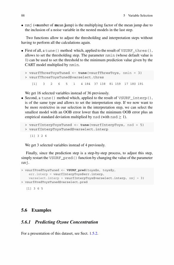
88 5 Variable Selection
• nmj (=number of mean jump) is the multiplying factor of the mean jump due tothe inclusion of a noise variable in the nested models in the last step.
Two functions allow to adjust the thresholding and interpretation steps withouthaving to perform all the calculations again.
• First of all, a tune()method which, applied to the result of VSURF_thres(),allows to set the thresholding step. The parameter nmin (whose default value is1) can be used to set the threshold to the minimum prediction value given by theCART model multiplied by nmin.
> vsurfThresToysTuned <- tune(vsurfThresToys, nmin = 3)> vsurfThresToysTuned$varselect.thres
[1] 3 2 6 5 1 4 184 37 138 81 159 17 180 191
We get 16 selected variables instead of 36 previously.• Second, a tune() method which, applied to the result of VSURF_interp(),is of the same type and allows to set the interpretation step. If we now want tobe more restrictive in our selection in the interpretation step, we can select thesmallest model with an OOB error lower than the minimum OOB error plus anempirical standard deviation multiplied by nsd (with nsd ≥ 1).
> vsurfInterpToysTuned <- tune(vsurfInterpToys, nsd = 5)> vsurfInterpToysTuned$varselect.interp
[1] 3 2 6
We get 3 selected variables instead of 4 previously.
Finally, since the prediction step is a step-by-step process, to adjust this step,simply restart the VSURF_pred() function by changing the value of the parameternmj.
> vsurfPredToysTuned <- VSURF_pred(toys$x, toys$y,err.interp = vsurfInterpToys$err.interp,varselect.interp = vsurfInterpToys$varselect.interp, nmj = 3)
> vsurfPredToysTuned$varselect.pred
[1] 3 6 5
5.6 Examples
5.6.1 Predicting Ozone Concentration
For a presentation of this dataset, see Sect. 1.5.2.

5.6 Examples 89
> library(VSURF)> data("Ozone", package = "mlbench")
After loading the data, the result of the entire selection procedure is obtained byusing the following command:
> set.seed(303601)> OzVSURF <- VSURF(V4 ˜ ., data = Ozone, na.action = na.omit)> summary(OzVSURF)
VSURF computation time: 1.4 mins
VSURF selected:9 variables at thresholding step (in 50.7 secs)5 variables at interpretation step (in 21.6 secs)5 variables at prediction step (in 9.8 secs)
> plot(OzVSURF, var.names = TRUE)
Let us now examine these results successively (illustrated in Fig. 5.4). To reflectthe order used in the definition of the variables, we first reorganize the variables atthe end of the procedure.
> number <- c(1:3, 5:13)> number[OzVSURF$varselect.thres]
[1] 9 8 12 1 11 10 5 7 13
variables
VI m
ean
V9 V12 V11 V5 V13 V3 V9 V12 V11 V5 V13 V3
variables
VI s
tand
ard
devi
atio
n
nested models
OO
B er
ror
V9 V12 V11 V5 V13
05
1020
0.05
0.20
0.35
1822
26
1822
26
predictive models
OO
B er
ror
V9 V8 V12 V1 V11
Fig. 5.4 Illustration of the results of VSURF(), Ozone data

90 5 Variable Selection
After the first step, the 3 variables of negative importance (variables 6, 3, and 2) areeliminated as expected.
> number[OzVSURF$varselect.interp]
[1] 9 8 12 1 11
Then, the interpretation procedure leads to the selection of the 5-variable model,which contains all the most important variables.
> number[OzVSURF$varselect.pred]
[1] 9 8 12 1 11
With the default settings, the prediction step does not remove any additionalvariables.
In fact, our strategy more or less assumes that there exist some useless variablesin the set of all initial variables, which is indeed the case in this dataset but not verysignificantly.
In addition, it should be noted here that our heuristics are clearly driven by pre-diction since the criterion for assessing the interest of a variable is closely related tothe quality of the prediction or more exactly to its increasing after permutation.
5.6.2 Analyzing Genomic Data
For a presentation of this dataset, see Sect. 1.5.3.Let us load the VSURF package, the vac18 data, and then create an object
geneExpr containing the gene expressions and an object stimu containing thestimuli to be predicted:
> library(VSURF)> data("vac18", package = "mixOmics")> geneExpr <- vac18$genes> stimu <- vac18$stimulation
The global procedurewith all parameters set to default values (note that the defaultvalue of mtry is p/3 even in classification, because as we have seen previously, thevalue of this parameter must be relatively high for high-dimensional problems) isobtained as follows:
> set.seed(481933)> vacVSURF <- VSURF(x = geneExpr, y = stimu)> summary(vacVSURF)
VSURF computation time: 3.1 mins

5.6 Examples 91
0 200 400 600 800 1000 0 200 400 600 800 1000
variables
VI m
ean
variables
VI s
tand
ard
devi
atio
n
0 20 40 60 80
0.00
00.
020
0.1
0.4
0.7
nested models
OO
B er
ror
2 4 6 8 100.
0000
0.00
150.
10.
40.
7
predictive models
OO
B er
ror
Fig. 5.5 Graphs illustrating the results of VSURF(), Vac18 data
VSURF selected:93 variables at thresholding step (in 1.7 mins)24 variables at interpretation step (in 1.3 mins)10 variables at prediction step (in 7.9 secs)
> plot(vacVSURF)
The first thresholding step keeps only 93 variables. This is reasonable given thegraph of the importance of the variables located at the top left of Fig. 5.5, which aspointed out in Sect. 4.5.3, illustrates a strong parsimony in the Vac18 data.
The interpretation step of VSURF() leads to the selection of 24 variables, whilethe prediction step selects 10 variables.
Finally, the names of the variables (identifiers of the biochip probes used to mea-sure gene expression) selected in the prediction step can be extracted as follows:
> probeSelPred <- colnames(geneExpr)[vacVSURF$varselect.pred]> probeSelPred
[1] "ILMN_1691156" "ILMN_2124802" "ILMN_2102693" "ILMN_1736939"[5] "ILMN_3252733" "ILMN_2188204" "ILMN_1658396" "ILMN_1663032"[9] "ILMN_3301824" "ILMN_2067444"
Computing timeThe VSURF() function can be run in parallel using the following command:

92 5 Variable Selection
> set.seed(627408, kind = "L’Ecuyer-CMRG")> vacVSURFpara <- VSURF(x = geneExpr, y = stimu, parallel = TRUE,
ncores = 3, clusterType = "FORK")> summary(vacVSURFpara)
VSURF computation time: 1.5 mins
VSURF selected:97 variables at thresholding step (in 45.9 secs)23 variables at interpretation step (in 38 secs)13 variables at prediction step (in 7 secs)
VSURF ran in parallel on a PSOCK cluster and used 3 cores
We observe in this example a factor of about 2 in terms of saving execution timeby using 3 cores instead of 1.

References
Alfaro, E., Gámez, M., & García, N. (2013). adabag: An R package for classification with boostingand bagging. Journal of Statistical Software, 54(2), 1–35.
Archer, K. J., & Kimes, R. V. (2008). Empirical characterization of random forest variable impor-tance measures. Computational Statistics and Data Analysis, 52(4), 2249–2260.
Azen, R., & Budescu, D. V. (2003). The dominance analysis approach for comparing predictors inmultiple regression. Psychological Methods, 8(2), 129.
Bach, F. R. (2008). Bolasso:model consistent lasso estimation through the bootstrap. InProceedingsof the 25th international conference on machine learning (pp. 33–40). ACM.
Biau, G. (2012). Analysis of a random forests model. Journal of Machine Learning Research,13(38), 1063–1095.
Bobbia,M., Jollois, F.-X., Poggi, J.-M.,&Portier, B. (2011). Quantifying local and background con-tributions to PM10 concentrations in Haute-Normandie, using random forests. Environmetrics,22(6), 758–768.
Boulesteix, A.-L., Janitza, S., Kruppa, J., &König, I. R. (2012). Overview of random forest method-ology and practical guidance with emphasis on computational biology and bioinformatics.WileyInterdisciplinary Reviews: Data Mining and Knowledge Discovery, 2(6), 493–507.
Breiman, L. (1996). Bagging predictors. Machine Learning, 24(2), 123–140.Breiman, L. (1998). Arcing classifier. The Annals of Statistics, 26(3), 801–849.Breiman, L. (2000). Randomizing outputs to increase prediction accuracy.Machine Learning, 40(3),229–242.
Breiman, L. (2001). Random forests. Machine Learning, 45(1), 5–32.Breiman, L., & Friedman, J. H. (1985). Estimating optimal transformations for multiple regressionand correlation. Journal of the American Statistical Association, 80(391), 580–598.
Breiman, L., Friedman, J., Olshen, R., & Stone, C. (1984). Classification and regression trees. NewYork: Chapman and Hall.
Cadenas, J. M., Carmen Garrido, M., &Martínez, R. (2013). Feature subset selection filter-wrapperbased on low quality data. Expert Systems with Applications, 40(16), 6241–6252.
Chen, C., Liaw, A., & Breiman, L. (2004).Using random forest to learn imbalanced data (Vol. 110,pp. 1–12). Berkeley: University of California.
Core Team, R. (2018). R: A Language and Environment for Statistical Computing. Vienna, Austria:R Foundation for Statistical Computing.
Cutler, A. (2010). Remembering Leo Breiman. The Annals of Applied Statistics, 4(4), 1621–1633.
© Springer Nature Switzerland AG 2020R. Genuer and J.-M. Poggi, Random Forests with R, Use R!,https://doi.org/10.1007/978-3-030-56485-8
93

94 References
Díaz-Uriarte, R., & Alvarez De Andres, S. (2006). Gene selection and classification of microarraydata using random forest. BMC Bioinformatics, 7(1), 3.
Dietterich, T.G. (2000). Ensemblemethods inmachine learning. Internationalworkshoponmultipleclassifier systems (pp. 1–15). Berlin: Springer.
Fan, J., & Lv, J. (2008). Sure independence screening for ultrahigh dimensional feature space.Journal of the Royal Statistical Society: Series B (Statistical Methodology), 70(5), 849–911.
Fellinghauer, B., Bühlmann, P., Ryffel, M., Von Rhein, M., & Reinhardt, J. D. (2013). Stablegraphical model estimation with random forests for discrete, continuous, and mixed variables.Computational Statistics and Data Analysis, 64, 132–152.
Fernández-Delgado, M., Cernadas, E., Barro, S., & Amorim, D. (2014). Do we need hundreds ofclassifiers to solve real world classification problems. Journal of Machine Learning Research,15(1), 3133–3181.
Freund, Y., & Schapire, R. E. (1997). A decision-theoretic generalization of on-line learning andan application to boosting. Journal of Computer and System Sciences, 55(1), 119–139.
Friedman, J. H. (1991). Multivariate adaptive regression splines. The Annals of Statistics, 1–67.Genuer, R., Michel, V., Eger, E., & Thirion, B. (2010a). Random forests based feature selection fordecoding fMRI data. In Proceedings COMPSTAT (Vol. 267, pp. 1–8).
Genuer, R., Poggi, J.-M., & Tuleau-Malot, C. (2018). VSURF: Variable Selection Using RandomForests. R package version, 1, 4.
Genuer, R., Poggi, J.-M., & Tuleau, C. (2008). Random forests: some methodological insights.arXiv:0811.3619.
Genuer, R., Poggi, J.-M., & Tuleau-Malot, C. (2010b). Variable selection using random forests.Pattern Recognition Letters, 31(14), 2225–2236.
Genuer, R., Poggi, J.-M., & Tuleau-Malot, C. (2015). VSURF: An R package for variable selectionusing random forests. The R Journal, 7(2), 19–33.
Gey, S. (2002). Bornes de risque, détection de ruptures, boosting: trois thèmes statistiques autourde CART en régression. Ph.D. thesis, Paris 11, Orsay.
Ghattas, B. (1999). Prévisions des pics d’ozone par arbres de régression, simples et agrégés parbootstrap. Revue de Statistique Appliquée, 47(2), 61–80.
Ghattas, B. (2000). Agrégation d’arbres de classification. Revue de Statistique Appliquée, 48(2),85–98.
Ghattas, B., & Ben Ishak, A. (2008). Sélection de variables pour la classification binaire en grandedimension: comparaisons et application aux données de biopuces. Journal de la Société FrançaiseDe Statistique, 149(3), 43–66.
Giraud, C. (2014). Introduction to high-dimensional statistics, (Vol. 138). CRC Press.Goldstein, B. A., Hubbard, A. E., Cutler, A., & Barcellos, L. F. (2010). An application of randomforests to a genome-wide association dataset: methodological considerations and new findings.BMC Genetics, 11(1), 1.
Gregorutti, B. (2016). RFgroove: Importance Measure and Selection for Groups of Variables withRandom Forests. R package version, 1, 1.
Gregorutti, B., Michel, B., & Saint-Pierre, P. (2013). Correlation and variable importance in randomforests. Statistics and Computing, 1–20.
Gregorutti, B., Michel, B., & Saint-Pierre, P. (2015). Grouped variable importance with randomforests and application to multiple functional data analysis. Computational Statistics and DataAnalysis, 90, 15–35.
Grömping, U. (2015). Variable importance in regression models. Wiley Interdisciplinary Reviews:Computational Statistics, 7(2), 137–152.
Guyon, I., Weston, J., Barnhill, S., & Vapnik, V. (2002). Gene selection for cancer classificationusing support vector machines.Machine Learning, 46(1–3), 389–422.
Hapfelmeier, A., & Ulm, K. (2012). A new variable selection approach using random forests.Computational Statistics and Data Analysis, 60, 50–69.
Ho, T.K. (1998). The random subspacemethod for constructing decision forests. IEEETransactionson Pattern Analysis and Machine Intelligence, 20(8), 832–844.

References 95
Hothorn, T., Hornik, K., Strobl, C., and Zeileis, A. (2017). party: A Laboratory for RecursivePartytioning. R package version 1.2–3.
Hothorn, T., Bühlmann, P., Dudoit, S., Molinaro, A., & Van Der Laan, M. J. (2006). Survivalensembles. Biostatistics, 7(3), 355–373.
Ishwaran, H., & Kogalur, U. (2017). Random Forests for Survival, Regression, and Classification(RF-SRC). R package version, 2(5), 1.
Ishwaran, H., Kogalur, U. B., Blackstone, E. H., & Lauer, M. S. (2008). Random survival forests.The Annals of Applied Statistics, 841–860.
Jollois, F.-X., Poggi, J.-M., & Portier, B. (2009). Three non-linear statistical methods for analyzingPM10 pollution in Rouen area. Case Studies In Business, Industry and Government Statistics,3(1), 1–17.
Karatzoglou, A., Smola, A., Hornik, K., & Zeileis, A. (2004). kernlab–an S4 package for kernelmethods in R. Journal of Statistical Software, 11(9), 1–20.
Kass, G. V. (1980). An exploratory technique for investigating large quantities of categorical data.Applied statistics, 119–127.
Le Cao, K.-A., Rohart, F., Gonzalez, I., & with key contributors Benoit Gautier, S. D., Bartolo, F.,contributions from Pierre Monget, Coquery, J., Yao, F., & Liquet., B., (2017). mixOmics: OmicsData Integration Project. R package version, 6(3), 1.
Lê Cao, K.-A., Gonçalves, O., Besse, P., & Gadat, S. (2007). Selection of biologically relevantgenes with a wrapper stochastic algorithm. Statistical Applications in Genetics and MolecularBiology, 6(1),
Leisch, F. & Dimitriadou, E. (2010).mlbench: Machine Learning Benchmark Problems. R packageversion 2.1–1.
Liaw, A. & Wiener, M. (2018). randomForest: Breiman and Cutler’s Random Forests for Classifi-cation and Regression. R package version 4.6–14.
Liaw,A.,&Wiener,M. (2002). Classification and regression by randomForest.RNews, 2(3), 18–22.Loh,W.-Y. (2014). Fifty years of classification and regression trees. International Statistical Review,82(3), 329–348.
Louppe, G., Wehenkel, L., Sutera, A., & Geurts, P. (2013). Understanding variable importances inforests of randomized trees. Advances in Neural Information Processing Systems, 431–439.
Meinshausen, N., & Bühlmann, P. (2010). Stability selection. Journal of the Royal Statistical Soci-ety: Series B (Statistical Methodology), 72(4), 417–473.
Milborrow, S. (2018). rpart.plot: Plot ’rpart’ Models: An Enhanced Version of ’plot.rpart’. Rpackage version 2.2.0.
Olshen, R. (2001). A conversation with Leo Breiman. Statistical Science, 184–198.Patil, D. V., & Bichkar, R. (2012). Issues in optimization of decision tree learning: A survey.International Journal of Applied Information Systems, 3(5),
Peters, A. & Hothorn, T. (2017). ipred: Improved Predictors. R package version 0.9–6.Poggi, J.-M. & Tuleau, C. (2006). Classification supervisée en grande dimension. application àl’agrément de conduite automobile. Revue de Statistique Appliquée, 54(4), 41–60.
Prasad,A.M., Iverson, L.R.,&Liaw,A. (2006).Newer classification and regression tree techniques:Bagging and random forests for ecological prediction. Ecosystems, 9(2), 181–199.
Questier, F., Put, R., Coomans, D., Walczak, B., & Vander Heyden, Y. (2005). The use of CART andmultivariate regression trees for supervised and unsupervised feature selection. Chemometricsand Intelligent Laboratory Systems, 76(1), 45–54.
Quinlan, J. R. (1993). C4. 5: Programming for machine learning. Morgan Kauffmann.Rakotomamonjy, A. (2003). Variable selection using SVM-based criteria. Journal of MachineLearning Research, 3, 1357–1370.
Ramosaj, B. & Pauly, M. (2019). Asymptotic unbiasedness of the permutation importance measurein random forest models. arXiv:1912.03306.
Ripley, B. (2018). tree: Classification and Regression Trees. R package version 1.0–39.Segal, M., & Xiao, Y. (2011). Multivariate random forests. Wiley Interdisciplinary Reviews: DataMining and Knowledge Discovery, 1(1), 80–87.

96 References
Seligman, M. (2017). Rborist: Extensible, Parallelizable Implementation of the Random ForestAlgorithm. R package version 0.1–7.
Strobl, C., Boulesteix, A.-L., Zeileis, A., & Hothorn, T. (2007). Bias in random forest variableimportance measures: Illustrations, sources and a solution. BMC Bioinformatics, 8(1), 25.
Strobl, C., Boulesteix, A.-L., Kneib, T., Augustin, T., & Zeileis, A. (2008). Conditional variableimportance for random forests. BMC Bioinformatics, 9(1), 307.
Therneau, T. &Atkinson, B. (2018). rpart: Recursive Partitioning and Regression Trees. R packageversion 4.1–13.
Thiébaut, R., Liquet, B., Hocini, H., Hue, S., Richert, L., Raimbault,M., et al. (2012). A newmethodfor integrated analysis applied to gene expression and cytokines secretion in response to LIPO-5vaccine in HIV-negative volunteers. Retrovirology, 9(Suppl 2), P121.
Tibshirani, R. (1996). Regression shrinkage and selection via the lasso. Journal of the Royal Sta-tistical Society: Series B (Statistical Methodology), 267–288.
Vapnik, V. (2013). The nature of statistical learning theory. Springer Science and Business Media.Verikas, A., Gelzinis, A., & Bacauskiene, M. (2011). Mining data with random forests: A surveyand results of new tests. Pattern Recognition, 44(2), 330–349.
Wallard, H. (2015). Analyse des leviers. Effets de colinéarité et hiérarchisation des impacts dansles études de marché et sociales. Ph.D. thesis, CNAM, Paris.
Welling, S. H., Refsgaard, H. H., Brockhoff, P. B., & Clemmensen, L. H. (2016). Forest floorvisualizations of random forests. arXiv:1605.09196.
Weston, J., Elisseeff, A., Schölkopf, B., & Tipping, M. (2003). Use of the zero norm with linearmodels and kernel methods. The Journal of Machine Learning Research, 3, 1439–1461.
Wright, M. N. (2017). ranger: A Fast Implementation of Random Forests. R package version, (8),Wu, X., Kumar, V., Quinlan, J. R., Ghosh, J., Yang, Q., Motoda, H., et al. (2008). Top 10 algorithmsin data mining. Knowledge and information systems, 14(1), 1–37.

Index
AAggregation, 33
BBagging, 2, 37Bootstrap, 35
CCART, 9
competing split, 22maximal tree, 10pruning, 13splitting, 11surrogate split, 23
Cross-validation, 15, 42V -fold, 15, 30
DDecision tree
CART, 9
MMissing data, 23, 28, 47Model selection
penalization, 14
OOne standard deviation rule, 80OOB error, 42
out-of-bag, 42, 80
PPackage
randomForest, 41–46ranger, 52rpart, 16–22VSURF, 81–88
Predictor, 3
RRandom forests, 33
partial effects, 52random inputs, 39
Recursive partitioning, 10Regression, 3Resampling
bootstrap, 35subsampling, 78
R functionsrandomForest(), 37, 41–46
partialPlot(), 53, 69plot(), 43predict(), 38, 42varImpPlot(), 59
rpart(), 16–17plot(), 17plotcp(), 18predict(), 22print(), 16–17prune(), 19rpart.control(), 16, 17, 30summary(), 23–24text(), 17
set.seed(), 6, 17, 85VSURF(), 81, 84, 87
plot(), 81summary(), 81
© Springer Nature Switzerland AG 2020R. Genuer and J.-M. Poggi, Random Forests with R, Use R!,https://doi.org/10.1007/978-3-030-56485-8
97

98 Index
tune(), 88VSURF_interp(), 83VSURF_pred(), 84, 88VSURF_thres(), 83
SStability, 1, 34
Supervised classification, 3
VVariable importance, 25, 57–61Variable selection, 77