robot localization for first robotics...robot localization for first robotics april 16, 2013 a major...
TRANSCRIPT
Robot Localization for FIRST Robotics
April 16, 2013
A Major Qualifying Project Report
Submitted to the faculty of
WORCESTER POLYTECHNIC INSTITUTE
In partial fulfillment of the requirements for the
Degree of Bachelor of Science in
Electrical & Computer Engineering and Robotics Engineering
By:
Scott Burger
Adam Moriarty
Samuel Patterson
Daniel Riches
Advisers:
Dr. David Cyganski
Dr. R. James Duckworth
Project Number: MQPDC1201

ii
Acknowledgements
We would like acknowledge the
contributions of those who helped make this project a success:
Professors Cyganski and Duckworth for always guiding us toward improving our work,
providing insightful advice, and for providing the inspiration for this project.
Professor Miller for his experience working with FIRST Robotics and his help as we defined our
system requirements.
Technician Bob Boisse for soldering the fine-pitch components to the camera PCB for us.
Kevin Arruda for getting up before dawn to teach how to use the laser cutter to make the case for
our embedded system.

iii
Abstract
The goal of this project is to develop a camera-based system that can determine the (x,y)
coordinates of one or more robots during FIRST Robotics Competition game play and transmit
this information to the robots. The intent of the system is to introduce an interesting new
dynamic to the competition for both the autonomous and user guided parts of play. To
accomplish this, robots are fitted with custom matrix LED beacons. Two to six cameras may
then capture images of the field while a FPGA embedded system at each camera performs image
processing to identify the beacons. This information is sent to a master computer which
combines the six images to reconstruct robot coordinates. The effort included simulating camera
imaging, designing and developing a beacon system, implementing interfaces and image
processing algorithms on an FPGA, meshing image data from multiple sources, and deploying a
functional prototype.
iv
Executive Summary
This project involved the design and construction of a location tracking system for robots
during FIRST Robotics Competitions (FRC). FRC is a large annual international competition
between high school teams organized by FIRST, in an effort to expose high school students to
engineering challenges. In preparation for the competition, students have 6 weeks to design and
build a robot to play a game developed by FIRST. Each year, the game is changed to present a
new challenge for contestants. In the past, robots have performed tasks in an arena such as
throwing basketballs into hoops, hanging objects in a certain order, and throwing Frisbees.
We designed and implemented a low-cost camera-based robot localization system to add
a new dynamic to FRC. This system sends the robots their locations in real-time, which allows
teams to enhance the capabilities of their robot, and allows FIRST to provide new, more
complicated challenges. For instance, teams could experiment with more precise control when
launching objects towards goals by knowing not only what direction the goal is in, but how far
away the goal is. It also opens the door to having longer autonomous game-play periods with
more advanced path planning requirements.
To realize this dynamic, our robot localization system uses custom programmable LED
beacons that provide unique patterns for each of the robots for visual identification. The beacons
were made using a colored LED matrix connected to a microcontroller that controls the matrix
pattern via a custom PCB that we designed. Each robot in the arena is fitted with a beacon and
multiple cameras placed in specific locations around the arena are capable of viewing the
beacons. The camera images are processed to identify the robots in the image, and each robot's
position is calculated from these images.
v
Each of the six cameras on the edges of the arena is connected to an FPGA development
board via a custom PCB that we also designed for this project to form a camera/FPGA vision
subsystem. Each camera sends image frames to the FPGA, where the frames are processed,
stored, and interpreted in order to locate and identify the beacons within the image. Then, the
information about each detected beacon from each of the vision subsystems is sent to a central
PC where the physical coordinate reconstruction is performed.
To provide reliable information to the PC, the FPGAs perform a number of critical
operations on the incoming frames. First, the data format of the incoming frames is converted
from YUV to RGB using a color space converter. Next, a color filter stage filters and normalizes
the colors in the image for enhanced performance during the identification process. Next, the
modified frame is stored in RAM. The FPGA logic was designed in Verilog using Xilinx design
tools. A soft-core Microblaze microprocessor was also generated inside the FPGA that searches
through the RAM to find pixels that had passed the filtering stage, and then interprets them to
find the centers of each beacon. Beacons that are found are then compared to the expected
signature of each unique pattern in order to determine which beacon corresponds to which robot.
Finally the location of the center of each beacon within the image plane is sent to the
central PC with an associated unique ID. Using algorithms we implemented, the pixel
coordinates of each received beacon are mapped to locations in the arena. The calculated
coordinates are transmitted wirelessly to the robots during the competition.
The system we designed has been successfully tested and implemented using a single
beacon, FPGA/camera vision subsystem, and PC. The full scale tests we performed indicate that
our system can calculate the location of the beacons accurately to within eight inches
consistently. The system is capable of running in real time, and the final step required to deploy

vi
the system is to duplicate the hardware and synchronize communication so there are six
camera/FPGA subsystems running at once.
vii
Table of Contents
Acknowledgements ......................................................................................................................... ii
Abstract .......................................................................................................................................... iii
Executive Summary ....................................................................................................................... iv
Table of Contents .......................................................................................................................... vii
Table of Figures ............................................................................................................................. xi
Table of Tables ............................................................................................................................ xvi
Chapter 1: Introduction ................................................................................................................... 1
Chapter 2: Background ................................................................................................................... 6
2.1: The FIRST Robotics Arena ................................................................................................. 6
2.2: Image Basics ........................................................................................................................ 7
2.3: Tracking Methods for Robot Detection and Identification .................................................. 7
2.3.1: Elevated Cameras with Color Detection and Thresholding.......................................... 8
2.3.2: Colored Pattern Recognition ....................................................................................... 10
2.4: Number of Cameras ........................................................................................................... 11
2.5: Mapping Pixels Onto the Arena......................................................................................... 12
2.5.1: From ends of the arena................................................................................................ 13
2.5.2: Using an Overhead Camera ........................................................................................ 16
2.5.3: Quantifying Perspective Distortion ............................................................................ 17
2.6: Image Processing Algorithm ............................................................................................. 20
viii
Chapter 3: System Design ............................................................................................................. 23
3.1: Camera ............................................................................................................................... 24
3.1.1: Camera Resolution ...................................................................................................... 24
3.1.2: Camera Interface ......................................................................................................... 26
3.1.3: Camera Specifications ................................................................................................ 26
3.2: LED Beacon ....................................................................................................................... 28
3.3: Image Acquisition and Processing ..................................................................................... 28
3.4: Beacon Location Reconstruction ....................................................................................... 30
Chapter 4: Modules for Testing .................................................................................................... 31
4.1: Camera Model.................................................................................................................... 31
4.2: VGA Display ..................................................................................................................... 31
4.3: Imaging Model ................................................................................................................... 32
Chapter 5: System Implementation ............................................................................................... 39
5.1: Tracking Beacon ................................................................................................................ 39
5.1.1: Requirements .............................................................................................................. 39
5.1.2: Design Choices and Considerations ........................................................................... 39
5.1.3: Tracking Beacon Design ............................................................................................. 41
5.1.4: LED Matrix Controller ............................................................................................... 43
5.1.5: Beacon Implementation .............................................................................................. 44
5.1.6: Testing ........................................................................................................................ 47
ix
5.2: Camera PCB ...................................................................................................................... 49
5.2.1: PCB Design................................................................................................................. 49
5.3: I2C Interface ....................................................................................................................... 52
5.4: Camera Interface ................................................................................................................ 57
5.5: Beacon Filter ...................................................................................................................... 58
5.5.1: Color Space Converter ................................................................................................ 58
5.5.2: Color Filter .................................................................................................................. 61
5.6: RAM Interface ................................................................................................................... 63
5.6.1: RAM Configuration .................................................................................................... 63
5.6.2: Read and Write Operations ......................................................................................... 66
5.6.3: System Interface ......................................................................................................... 69
5.7: Interfacing Submodules ..................................................................................................... 71
5.8: Image Processing ............................................................................................................... 72
5.8.1: Implementation ........................................................................................................... 72
5.8.2: Testing ........................................................................................................................ 74
5.9: Reconstructing Locations from Images.......................................................................... 80
5.9.1: Requirements .......................................................................................................... 81
5.9.2: Implementation ....................................................................................................... 81
5.9.3: Testing ........................................................................................................................ 84
5.10: Calibration Algorithm ...................................................................................................... 84
x
Chapter 6: System Testing ............................................................................................................ 89
Chapter 7: Conclusions ................................................................................................................. 94
7.1: Future Work ....................................................................................................................... 95
References ..................................................................................................................................... 97
Appendix A: Beacon Control Code .............................................................................................. 99
Appendix B: LED Matrix Controller Schematic ........................................................................ 106
Appendix C: Verilog Modules .................................................................................................... 107
Appendix D: Section of Image Processing Code ........................................................................ 113
Appendix E: Sample of Processing Code ................................................................................... 116
Appendix F: List of Materials ..................................................................................................... 118
xi
Table of Figures
Figure 1: LOGOMOTION Arena [1] ............................................................................................. 2
Figure 2: Camera Locations on FIRST Arena (Overhead View) ................................................... 4
Figure 3: Cameras around the FIRST arena ................................................................................... 4
Figure 4: FIRST Arena for 2013 [2] ............................................................................................... 6
Figure 5: Grayscale Pixel Intensity [3] ........................................................................................... 7
Figure 6: The Field with Cameras [4] ............................................................................................. 8
Figure 7: Using Thresholds to Convert Colored Images to Black And White [4] ......................... 9
Figure 8: An RGB Color Pattern [5] ............................................................................................. 10
Figure 9: Moving From Colored Image to Identification Step [5] ............................................... 11
Figure 10: An Image Frame Showing Separate Targets Being Recognized [5] ........................... 11
Figure 11: Multiple Cameras Tracking Objects [6] ...................................................................... 12
Figure 12: Camera View from One End of the Arena .................................................................. 13
Figure 13: Cross Section of the Scene .......................................................................................... 14
Figure 14: Cross Sectional View of the Scene with Two Cameras .............................................. 15
Figure 15: Cross Sectional View of the Scene with Two Cameras with Their Own Spaces to
Monitor ......................................................................................................................................... 16
Figure 16: Cross Section of the Scene with One Overhead Camera ............................................ 17
Figure 17: Aid for Calculation of Space Covered Per Pixel ......................................................... 18
Figure 18: Original Image (Left) and Filtered Image (Right) [7] ................................................. 20
Figure 19: Non-Background Pixel Identified [7] .......................................................................... 21
Figure 20: Line Comparison [7] ................................................................................................... 21
Figure 21: Example Requiring Merge [7] ..................................................................................... 22
xii
Figure 22: System Hierarchy ........................................................................................................ 24
Figure 23: Heat Map of Accuracy from a Corner ......................................................................... 25
Figure 24: Accuracy from Center of Sideline ............................................................................... 26
Figure 25: 24C1.3XDIG Camera Module [8] ............................................................................... 27
Figure 26: LED Matrix with PCB Controller and MSP430 ......................................................... 28
Figure 27: Image Acquisition and Image Processing Block Diagram .......................................... 29
Figure 28: VGA Display Testbench ............................................................................................. 32
Figure 29: Overhead View of Objects on Field Being Viewed By A Camera ............................. 33
Figure 30: Image of the Scene in Figure 29 Using Our Simple Camera Model ........................... 34
Figure 31: Actual Image Taken by Camera as Seen in Figure 29 ................................................ 34
Figure 32: Examples of Frame Transformations from B to F [9] ................................................. 35
Figure 33: Rotation of Q in frame (x,y,z) to Q' in frame (u,v,w) ................................................. 36
Figure 34: Accurate Simulation of setup in Figure 29 .................................................................. 37
Figure 35: Original Beacon Layout .............................................................................................. 40
Figure 36: LED Beacon Design .................................................................................................... 40
Figure 37: LED Matrix for Beacon Design .................................................................................. 41
Figure 38: Example of Illuminated Beacon .................................................................................. 42
Figure 39: Layout of Row/Column Grouping .............................................................................. 44
Figure 40: Prefabricated LED Matrix Controller PCB ................................................................. 45
Figure 41: Led Matrix Controller Assembled ............................................................................... 46
Figure 42: LED Matrix with PCB Controller and MSP430 ......................................................... 47
Figure 43: LED PCB Malfunction ................................................................................................ 47
Figure 44: Former Board Layout .................................................................................................. 48
xiii
Figure 45: Necessary Board Layout ............................................................................................. 48
Figure 46: LED Matrix Displaying Pattern 3 ............................................................................... 49
Figure 47: Custom Breakout PCB before Order ........................................................................... 50
Figure 48: Fabricated PCB............................................................................................................ 51
Figure 49: PCB with Camera Attached, Plugged Into Nexys3 Board .......................................... 51
Figure 50: Resolution and Frame Rate Chart [8] .......................................................................... 52
Figure 51: Register 0 Detail [8] .................................................................................................... 53
Figure 52: Reading Default Settings via I2C................................................................................. 54
Figure 53: Displaying Read Results to User ................................................................................. 54
Figure 54: Writing 0x40c3 to Register 0 ...................................................................................... 55
Figure 55: Reading 0x40c3 from Register 0 ................................................................................. 56
Figure 56: Results of Reading the Previously-Written Value of Register 0 ................................. 56
Figure 57: Data Format of Camera [8] ......................................................................................... 57
Figure 58: Camera Interface Block Diagram ................................................................................ 58
Figure 59: Color Space Converter Block Diagram ....................................................................... 60
Figure 60: Color Space Conversion Testbench ............................................................................ 61
Figure 61: Completed Beacon Filter Block Diagram ................................................................... 62
Figure 62: Unfiltered Image.......................................................................................................... 62
Figure 63: Filtered Image.............................................................................................................. 63
Figure 64: BCR Write Operation[10] ........................................................................................... 64
Figure 65: BCR Write Operation Testbench ................................................................................ 65
Figure 66: Burst Mode Write [10] ................................................................................................ 66
Figure 67: Burst Mode Read [10] ................................................................................................. 66
xiv
Figure 68: Write to Address 0 ....................................................................................................... 68
Figure 69: Read from Address 0 ................................................................................................... 68
Figure 70: Intended Write Operation ............................................................................................ 69
Figure 71: Portion of RAM after Write Operation ....................................................................... 69
Figure 72: Block Diagram of Integrated Modules ........................................................................ 72
Figure 73: MATLAB Patch Locator Test Image .......................................................................... 74
Figure 74: Results of MATLAB Patch Locator ............................................................................ 75
Figure 75: Debugging Microblaze access to RAM....................................................................... 76
Figure 76: Full Scale Test Image .................................................................................................. 77
Figure 77: Beacon Identifier Test Output ..................................................................................... 78
Figure 78: Beacon Requiring Merging ......................................................................................... 79
Figure 79: Image for Beacon Pattern Identification Test .............................................................. 79
Figure 80: Results of Beacon Pattern Identification Test ............................................................. 80
Figure 81: Resolving Beacon Positions Concept .......................................................................... 80
Figure 82: Overhead View of Location Reconstruction Theory .................................................. 83
Figure 83: Pitch and Z Pose Parameters, Side View .................................................................... 85
Figure 84: Roll Pose Parameter, View of Camera From Behind .................................................. 85
Figure 85: Yaw, X, Y Pose Parameters Shown, Overhead View of Camera ............................... 85
Figure 86: Error between Two Images ......................................................................................... 86
Figure 87: Reference Frames for Camera Calibration [12] .......................................................... 88
Figure 88: Camera/FPGA subsystem, case, and holster ............................................................... 90
Figure 89: Actual Beacon (98, 166) Compared to Reconstructed Location (106, 166) in Test 2.
Total Error: 8 Inches ..................................................................................................................... 91

xv
Figure 90: Actual Beacon (62, 132) Compared to Reconstructed Location (63, 134) in Test 2.
Total Error: 2 Inches ..................................................................................................................... 92
Figure 91: Larger Scale Test Results ............................................................................................ 92

xvi
Table of Tables
Table 1: Identification Patterns ..................................................................................................... 43
Table 2: BCR Settings .................................................................................................................. 65

1
Chapter 1: Introduction
The FIRST Robotics Competition (FRC) is a large international competition between
high school teams. It is organized by FIRST, which stands for “For Inspiration and Recognition
of Science and Technology.” This organization was founded in 1989 by Dean Kamen with the
goal of increasing appreciation of science and technology and offering students opportunities to
learn important skills be exposed to engineering practices. High school students are given six
weeks to build a robot that weighs less than 120 pounds and can operate both autonomously and
under wireless direction. These robots are given tasks to complete, and the team that completes
the task most effectively wins the competition.
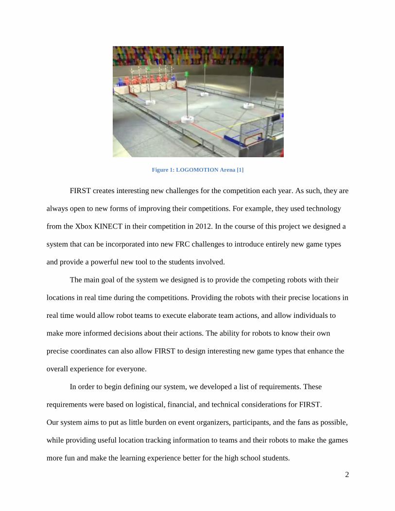
The games for the FRC are different every year. In 2011, the game was called
“LOGOMOTION.” In this game, robots were required to pick up pieces of the FIRST logo and
place them on a rack on the opposing team’s side of the arena in the same order as the logo.
Once this task is completed, the robots released a miniature robot which was capable of climbing
the posts within the arena. In 2012, the game was called “Rebound Rumble.” In this game, teams
used robots to toss basketballs into hoops on the opposing team’s side of the arena. There were
four hoops and the higher hoops awarded more points to the scorer. A typical FIRST arena
environment is shown in Figure 1below.
2
Figure 1: LOGOMOTION Arena [1]
FIRST creates interesting new challenges for the competition each year. As such, they are
always open to new forms of improving their competitions. For example, they used technology
from the Xbox KINECT in their competition in 2012. In the course of this project we designed a
system that can be incorporated into new FRC challenges to introduce entirely new game types
and provide a powerful new tool to the students involved.
The main goal of the system we designed is to provide the competing robots with their
locations in real time during the competitions. Providing the robots with their precise locations in
real time would allow robot teams to execute elaborate team actions, and allow individuals to
make more informed decisions about their actions. The ability for robots to know their own
precise coordinates can also allow FIRST to design interesting new game types that enhance the
overall experience for everyone.
In order to begin defining our system, we developed a list of requirements. These
requirements were based on logistical, financial, and technical considerations for FIRST.
Our system aims to put as little burden on event organizers, participants, and the fans as possible,
while providing useful location tracking information to teams and their robots to make the games
more fun and make the learning experience better for the high school students.

3
The first requirement for our system is that it is capable of consistently identifying all
robots individually. The data produced by our system would not be useful if it merely detected
the positions of unspecified robots. Adding the ability to identify robots as individuals ensures
that teams will be able to use the data we provide effectively.
In order for our tracking system to be useful, it must be accurate. To meet this
requirement, we aimed for our system to be accurate to within 3 inches. However, so long as the
system is relatively accurate, it will be of use to the competitors. We strove to make the system
as accurate as possible while keeping the overall cost of the system low enough for FIRST to
incorporate the system into their competitions.
Further, our system must not disrupt the flow of the FRC challenges. This means that our
system must be assembled and initialized quickly and seamlessly before a FIRST event begins.
Additionally, the system must be capable of functioning for an entire event without requiring
maintenance. Finally, our system must cost a reasonable amount so that organizers can afford to
utilize the system.
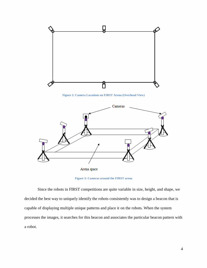
In our research, we determined that the most effective method for fulfilling the goals and
requirements of this system utilizes cameras. Based on simulations and other design
considerations, our design called for the use of six cameras. These cameras were placed around
the arena as can be seen in Figure 2 and Figure 3 below.
4
Figure 2: Camera Locations on FIRST Arena (Overhead View)
Figure 3: Cameras around the FIRST arena
Since the robots in FIRST competitions are quite variable in size, height, and shape, we
decided the best way to uniquely identify the robots consistently was to design a beacon that is
capable of displaying multiple unique patterns and place it on the robots. When the system
processes the images, it searches for this beacon and associates the particular beacon pattern with
a robot.

5
After we process the images from each camera, we combine the data from all of the
cameras to locate the robots in the arena. This is done using similar concepts to stereo-vision, but
with up to six cameras being integrated into the system. Using six camera stereo-vision also
allows the system to see robots that have traveled near obstacles that may obscure the ability of a
particular camera to see them.
The next chapter describes the background work that guided the design process. Chapter
3 will discuss the system design, and Chapter 4 will describe implementations we created to
facilitate system development. Chapter 5 will explain the details of our implementation, and
Chapter 6 will show the system tests we performed and their results. Finally in Chapter 7 we will
show the results of our tests and the conclusions we drew from these results.
6
Chapter 2: Background
This chapter describes the background work we carried out for the project. It includes
becoming familiar with the FIRST arena environment, investigating camera-based tracking
methods, investigating the geometry involved with mapping pixels onto a surface, and
investigating image processing algorithms.
2.1: The FIRST Robotics Arena
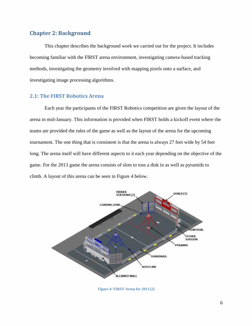
Each year the participants of the FIRST Robotics competition are given the layout of the
arena in mid-January. This information is provided when FIRST holds a kickoff event where the
teams are provided the rules of the game as well as the layout of the arena for the upcoming
tournament. The one thing that is consistent is that the arena is always 27 feet wide by 54 feet
long. The arena itself will have different aspects to it each year depending on the objective of the
game. For the 2013 game the arena consists of slots to toss a disk in as well as pyramids to
climb. A layout of this arena can be seen in Figure 4 below.
Figure 4: FIRST Arena for 2013 [2]
7
In previous years the field has had components such as ramps, racks and different pieces
of equipment that can either aid the teams or add more complexities to give the robots a more
difficult challenge.
2.2: Image Basics
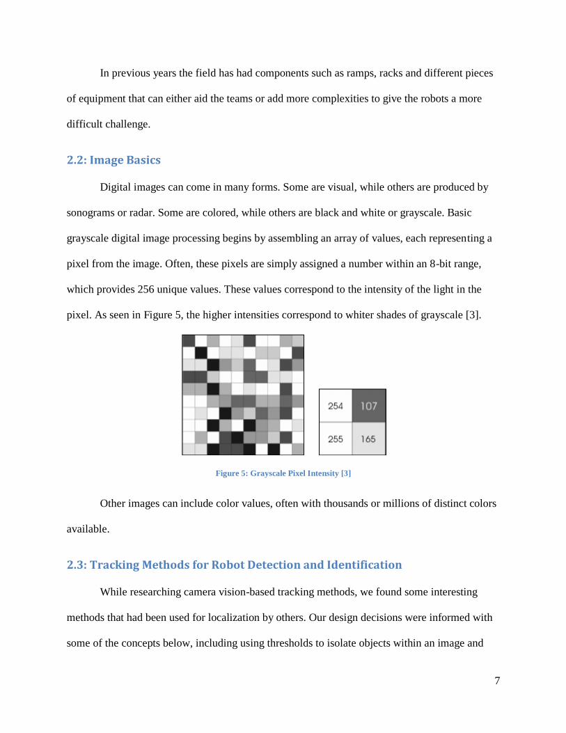
Digital images can come in many forms. Some are visual, while others are produced by
sonograms or radar. Some are colored, while others are black and white or grayscale. Basic
grayscale digital image processing begins by assembling an array of values, each representing a
pixel from the image. Often, these pixels are simply assigned a number within an 8-bit range,
which provides 256 unique values. These values correspond to the intensity of the light in the
pixel. As seen in Figure 5, the higher intensities correspond to whiter shades of grayscale [3].
Figure 5: Grayscale Pixel Intensity [3]
Other images can include color values, often with thousands or millions of distinct colors
available.
2.3: Tracking Methods for Robot Detection and Identification
While researching camera vision-based tracking methods, we found some interesting
methods that had been used for localization by others. Our design decisions were informed with
some of the concepts below, including using thresholds to isolate objects within an image and
8
using color pattern recognition. We also explored overhead camera use but found it to be overly
burdensome for FIRST.
2.3.1: Elevated Cameras with Color Detection and Thresholding
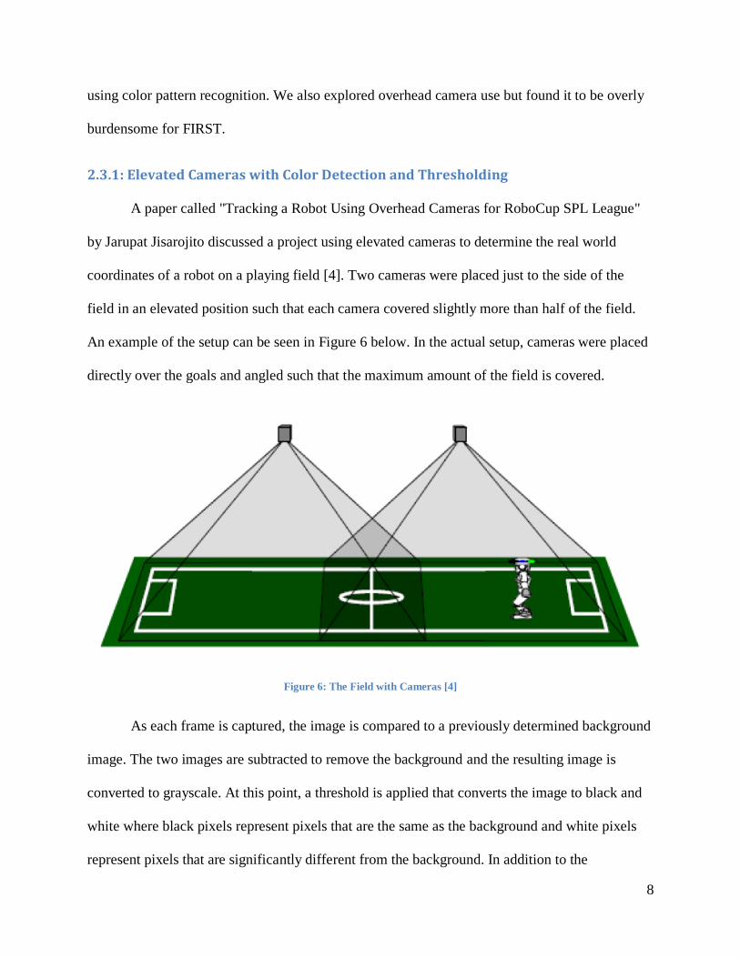
A paper called "Tracking a Robot Using Overhead Cameras for RoboCup SPL League"
by Jarupat Jisarojito discussed a project using elevated cameras to determine the real world
coordinates of a robot on a playing field [4]. Two cameras were placed just to the side of the
field in an elevated position such that each camera covered slightly more than half of the field.
An example of the setup can be seen in Figure 6 below. In the actual setup, cameras were placed
directly over the goals and angled such that the maximum amount of the field is covered.
Figure 6: The Field with Cameras [4]
As each frame is captured, the image is compared to a previously determined background
image. The two images are subtracted to remove the background and the resulting image is
converted to grayscale. At this point, a threshold is applied that converts the image to black and
white where black pixels represent pixels that are the same as the background and white pixels
represent pixels that are significantly different from the background. In addition to the
9
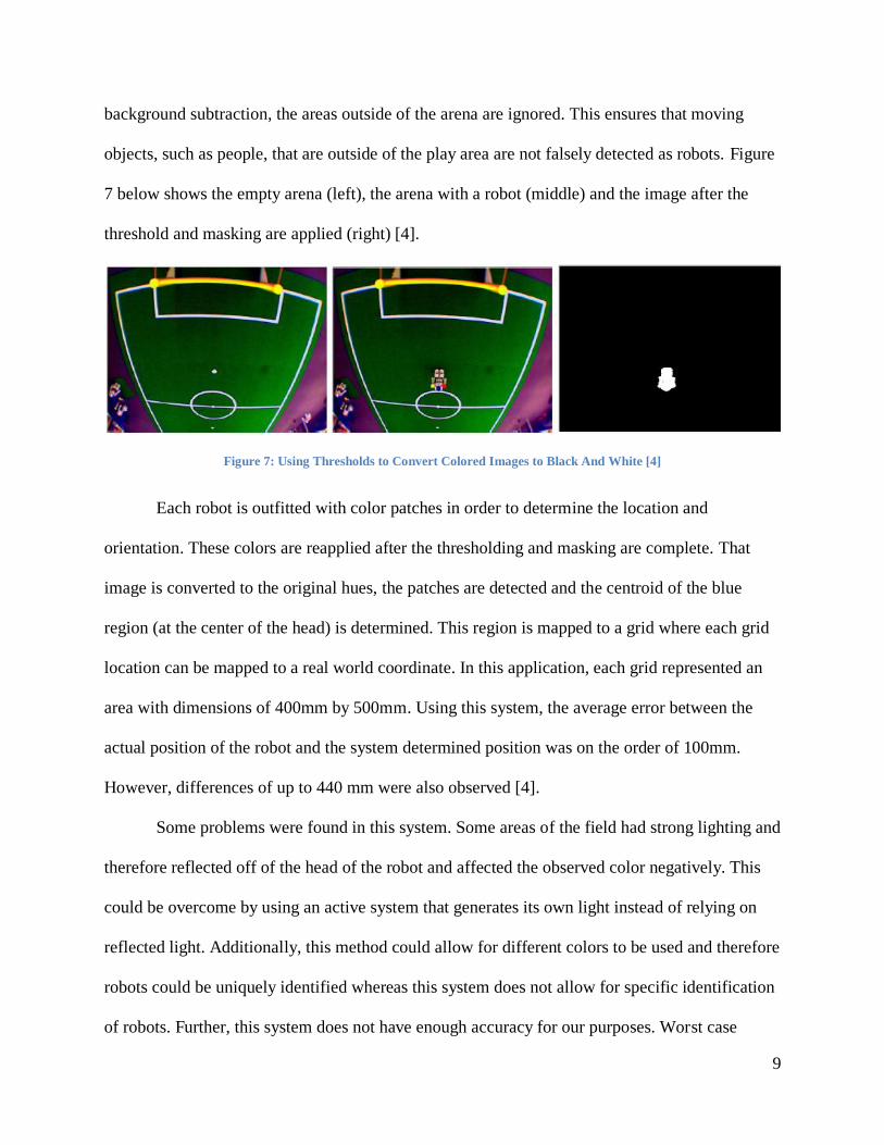
background subtraction, the areas outside of the arena are ignored. This ensures that moving
objects, such as people, that are outside of the play area are not falsely detected as robots. Figure
7 below shows the empty arena (left), the arena with a robot (middle) and the image after the
threshold and masking are applied (right) [4].
Figure 7: Using Thresholds to Convert Colored Images to Black And White [4]
Each robot is outfitted with color patches in order to determine the location and
orientation. These colors are reapplied after the thresholding and masking are complete. That
image is converted to the original hues, the patches are detected and the centroid of the blue
region (at the center of the head) is determined. This region is mapped to a grid where each grid
location can be mapped to a real world coordinate. In this application, each grid represented an
area with dimensions of 400mm by 500mm. Using this system, the average error between the
actual position of the robot and the system determined position was on the order of 100mm.
However, differences of up to 440 mm were also observed [4].
Some problems were found in this system. Some areas of the field had strong lighting and
therefore reflected off of the head of the robot and affected the observed color negatively. This
could be overcome by using an active system that generates its own light instead of relying on
reflected light. Additionally, this method could allow for different colors to be used and therefore
robots could be uniquely identified whereas this system does not allow for specific identification
of robots. Further, this system does not have enough accuracy for our purposes. Worst case
10
errors in the position of the robot were 17.6 inches. This issue could be resolved by using more
than two cameras. This would improve accuracy and would allow for redundancy in the case
where one robot occludes another from view [4].
2.3.2: Colored Pattern Recognition
A paper entitled “Robotracker – A System for Tracking Multiple Robots in Real Time”
by Alex Sirota discussed the use of a program to track multiple robots in an arena in real time
[5]. This application was aimed towards miniature robotic Lego cars which would move around
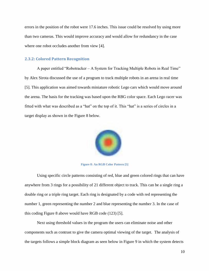
the arena. The basis for the tracking was based upon the RBG color space. Each Lego racer was
fitted with what was described as a “hat” on the top of it. This “hat” is a series of circles in a
target display as shown in the Figure 8 below.
Figure 8: An RGB Color Pattern [5]
Using specific circle patterns consisting of red, blue and green colored rings that can have
anywhere from 3 rings for a possibility of 21 different object to track. This can be a single ring a
double ring or a triple ring target. Each ring is designated by a code with red representing the
number 1, green representing the number 2 and blue representing the number 3. In the case of
this coding Figure 8 above would have RGB code (123) [5].
Next using threshold values in the program the users can eliminate noise and other
components such as contrast to give the camera optimal viewing of the target. The analysis of
the targets follows a simple block diagram as seen below in Figure 9 in which the system detects
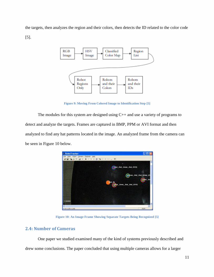
11
the targets, then analyzes the region and their colors, then detects the ID related to the color code
[5].
Figure 9: Moving From Colored Image to Identification Step [5]
The modules for this system are designed using C++ and use a variety of programs to
detect and analyze the targets. Frames are captured in BMP, PPM or AVI format and then
analyzed to find any hat patterns located in the image. An analyzed frame from the camera can
be seen in Figure 10 below.
Figure 10: An Image Frame Showing Separate Targets Being Recognized [5]
2.4: Number of Cameras
One paper we studied examined many of the kind of systems previously described and
drew some conclusions. The paper concluded that using multiple cameras allows for a larger
12
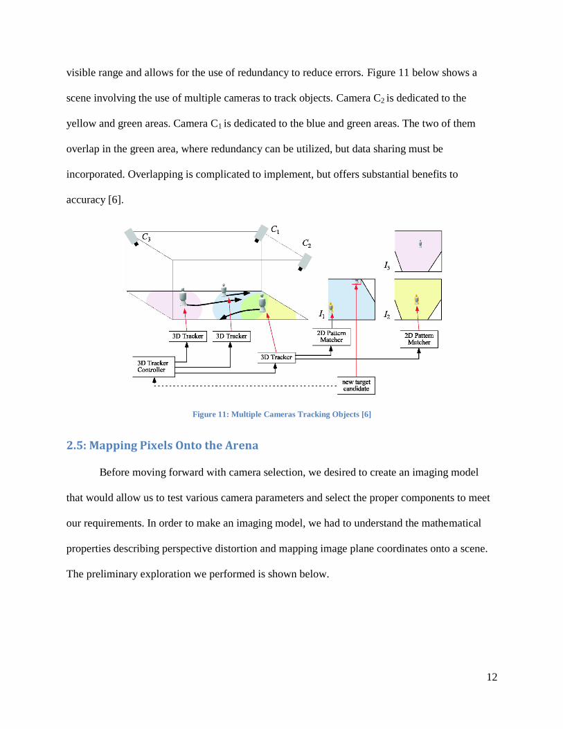
visible range and allows for the use of redundancy to reduce errors. Figure 11 below shows a
scene involving the use of multiple cameras to track objects. Camera C2 is dedicated to the
yellow and green areas. Camera C1 is dedicated to the blue and green areas. The two of them
overlap in the green area, where redundancy can be utilized, but data sharing must be
incorporated. Overlapping is complicated to implement, but offers substantial benefits to
accuracy [6].
Figure 11: Multiple Cameras Tracking Objects [6]
2.5: Mapping Pixels Onto the Arena
Before moving forward with camera selection, we desired to create an imaging model
that would allow us to test various camera parameters and select the proper components to meet
our requirements. In order to make an imaging model, we had to understand the mathematical
properties describing perspective distortion and mapping image plane coordinates onto a scene.
The preliminary exploration we performed is shown below.
13
2.5.1: From ends of the arena
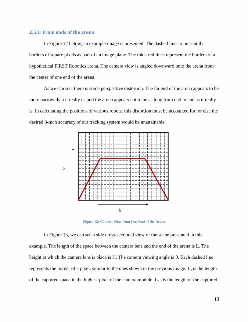
In Figure 12 below, an example image is presented. The dashed lines represent the
borders of square pixels as part of an image plane. The thick red lines represent the borders of a
hypothetical FIRST Robotics arena. The camera view is angled downward onto the arena from
the center of one end of the arena.
As we can see, there is some perspective distortion. The far end of the arena appears to be
more narrow than it really is, and the arena appears not to be as long from end to end as it really
is. In calculating the positions of various robots, this distortion must be accounted for, or else the
desired 3-inch accuracy of our tracking system would be unattainable.
Figure 12: Camera View from One End of the Arena
In Figure 13, we can see a side cross-sectional view of the scene presented in this
example. The length of the space between the camera lens and the end of the arena is L. The
height at which the camera lens is place is H. The camera viewing angle is θ. Each dashed line
represents the border of a pixel, similar to the ones shown in the previous image. Ln is the length
of the captured space in the highest pixel of the camera module. Ln-1 is the length of the captured
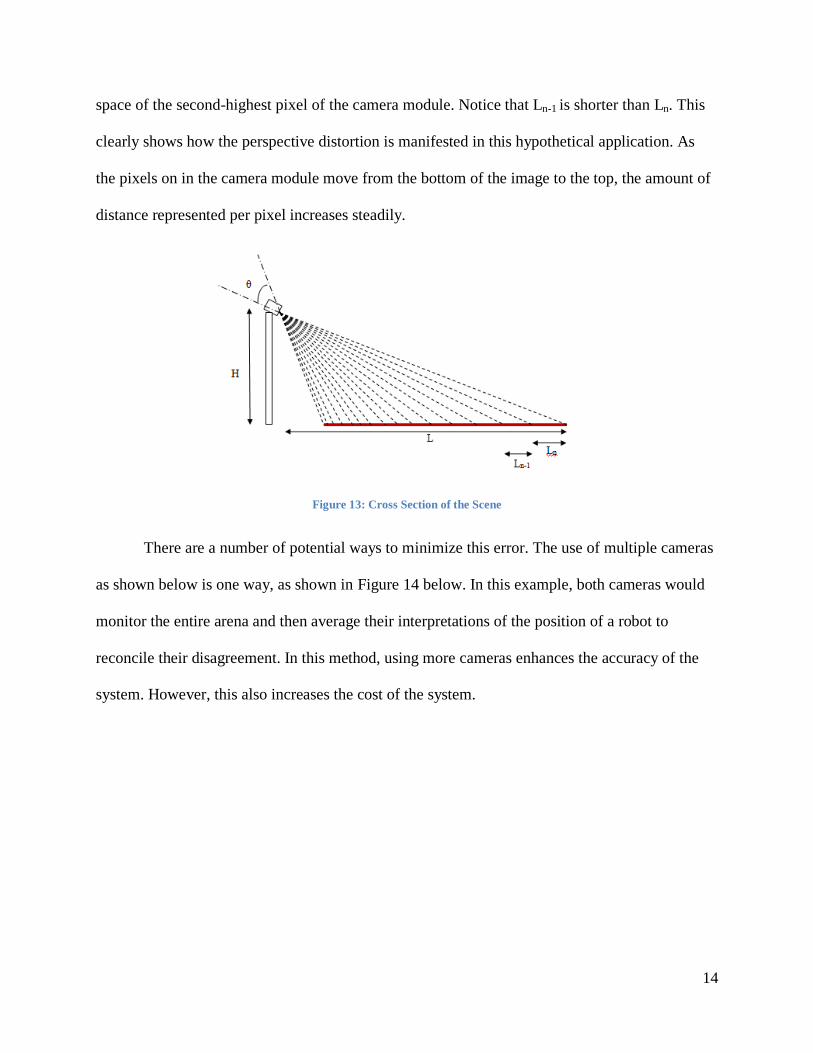
14
space of the second-highest pixel of the camera module. Notice that Ln-1 is shorter than Ln. This
clearly shows how the perspective distortion is manifested in this hypothetical application. As
the pixels on in the camera module move from the bottom of the image to the top, the amount of
distance represented per pixel increases steadily.
Figure 13: Cross Section of the Scene
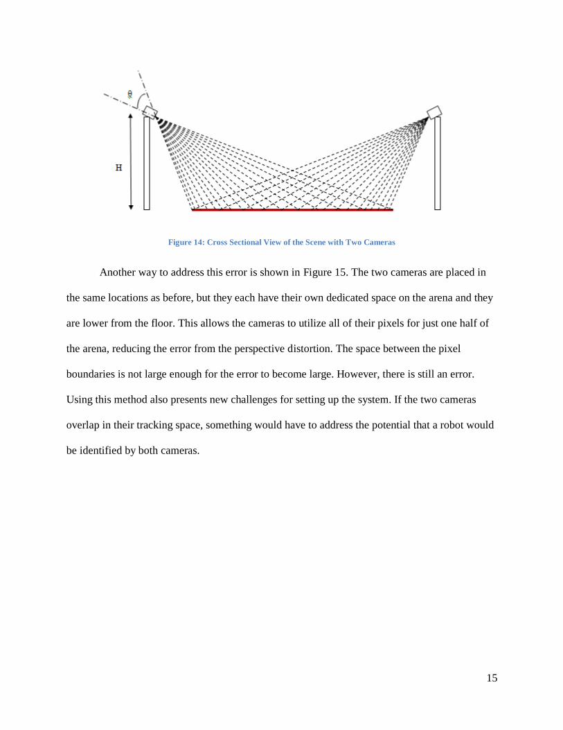
There are a number of potential ways to minimize this error. The use of multiple cameras
as shown below is one way, as shown in Figure 14 below. In this example, both cameras would
monitor the entire arena and then average their interpretations of the position of a robot to
reconcile their disagreement. In this method, using more cameras enhances the accuracy of the
system. However, this also increases the cost of the system.
15
Figure 14: Cross Sectional View of the Scene with Two Cameras
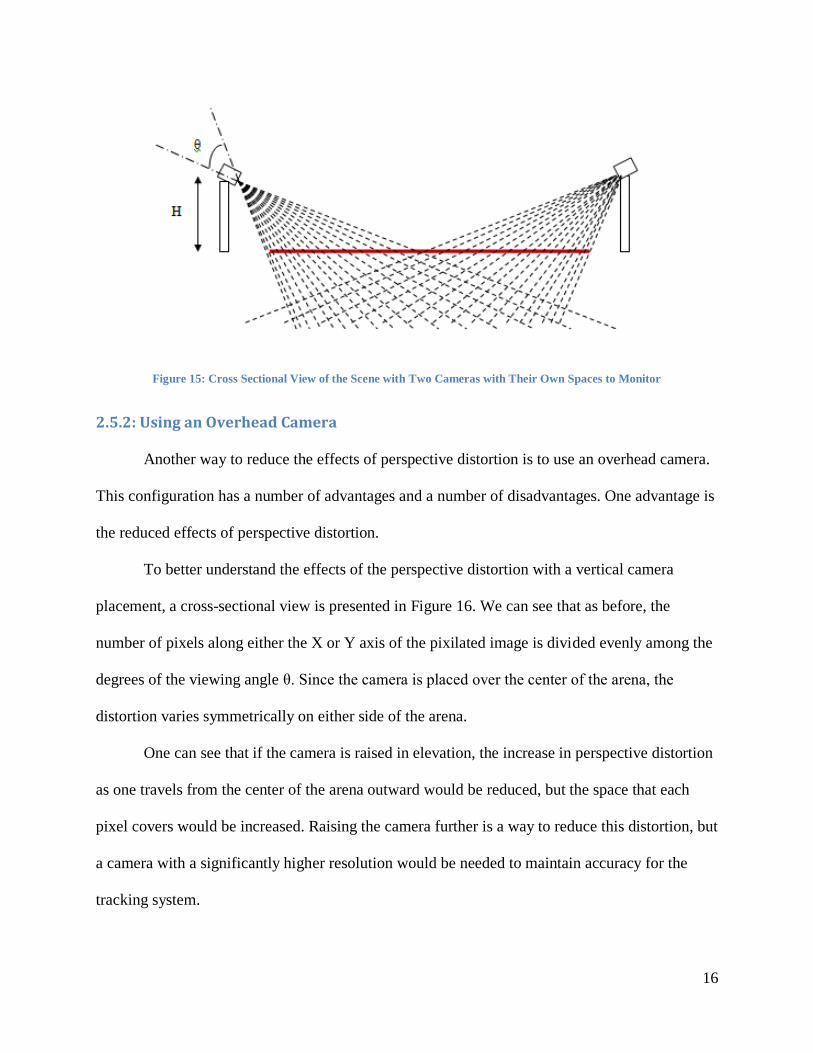
Another way to address this error is shown in Figure 15. The two cameras are placed in
the same locations as before, but they each have their own dedicated space on the arena and they
are lower from the floor. This allows the cameras to utilize all of their pixels for just one half of
the arena, reducing the error from the perspective distortion. The space between the pixel
boundaries is not large enough for the error to become large. However, there is still an error.
Using this method also presents new challenges for setting up the system. If the two cameras
overlap in their tracking space, something would have to address the potential that a robot would
be identified by both cameras.
16
Figure 15: Cross Sectional View of the Scene with Two Cameras with Their Own Spaces to Monitor
2.5.2: Using an Overhead Camera
Another way to reduce the effects of perspective distortion is to use an overhead camera.
This configuration has a number of advantages and a number of disadvantages. One advantage is
the reduced effects of perspective distortion.
To better understand the effects of the perspective distortion with a vertical camera
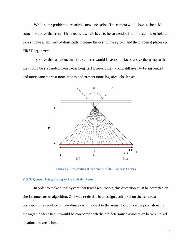
placement, a cross-sectional view is presented in Figure 16. We can see that as before, the
number of pixels along either the X or Y axis of the pixilated image is divided evenly among the
degrees of the viewing angle θ. Since the camera is placed over the center of the arena, the
distortion varies symmetrically on either side of the arena.
One can see that if the camera is raised in elevation, the increase in perspective distortion
as one travels from the center of the arena outward would be reduced, but the space that each
pixel covers would be increased. Raising the camera further is a way to reduce this distortion, but
a camera with a significantly higher resolution would be needed to maintain accuracy for the
tracking system.
17
While some problems are solved, new ones arise. The camera would have to be held
somehow above the arena. This means it would have to be suspended from the ceiling or held up
by a structure. This would drastically increase the cost of the system and the burden it places on
FIRST organizers.
To solve this problem, multiple cameras would have to be placed above the arena so that
they could be suspended from lower heights. However, they would still need to be suspended
and more cameras cost more money and present more logistical challenges.
Figure 16: Cross Section of the Scene with One Overhead Camera
2.5.3: Quantifying Perspective Distortion
In order to make a real system that tracks real robots, this distortion must be corrected on-
site in some sort of algorithm. One way to do this is to assign each pixel on the camera a
corresponding set of (x, y) coordinates with respect to the arena floor. Once the pixel showing
the target is identified, it would be compared with the pre-determined association between pixel
location and arena location.
18
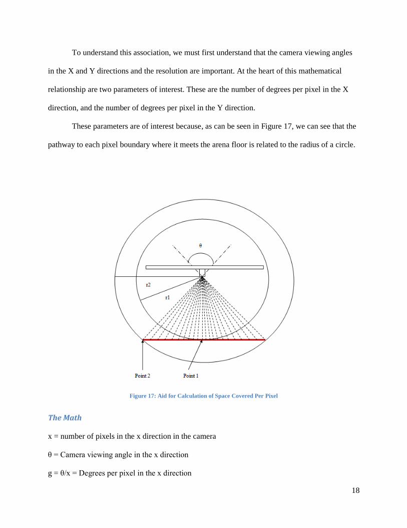
To understand this association, we must first understand that the camera viewing angles
in the X and Y directions and the resolution are important. At the heart of this mathematical
relationship are two parameters of interest. These are the number of degrees per pixel in the X
direction, and the number of degrees per pixel in the Y direction.
These parameters are of interest because, as can be seen in Figure 17, we can see that the
pathway to each pixel boundary where it meets the arena floor is related to the radius of a circle.
Figure 17: Aid for Calculation of Space Covered Per Pixel
The Math
x = number of pixels in the x direction in the camera
θ = Camera viewing angle in the x direction
g = θ/x = Degrees per pixel in the x direction

19
H = r1 = height of the camera
r2 = distance from camera lens to Point 2 in the x direction
L1 = length of the area between Point 1 and the first pixel boundary
L2 = length of the area between the first pixel boundary and the second pixel boundary
P = Pixels from the center of the image
We start with just one triangle, formed between Point 1, the camera lens, and the first
pixel boundary.
L1 = H * tan(g) (2.1)
The next triangle is formed between Point 1, the camera lens, and the second pixel
boundary.
L2 = H * tan(2g) (2.2)
Continuing further, the general relationship is
LN = H * tan(P * g) (2.3)
This relationship can be used to show the position of any pixel in an image, mapped to
the FIRST arena. To form the coordinates (x, y), the equations for the Y direction are the same,
but with different parameters, which are given by the camera.
Notes
Later, the above calculations were found to only be useful when mapping the pixels along
one-dimensional lines on the arena space. Further research was done to find a more robust
mathematical relationship between the image plane and arena surface, and it is discussed in
Chapter 4.3.
20
2.6: Image Processing Algorithm
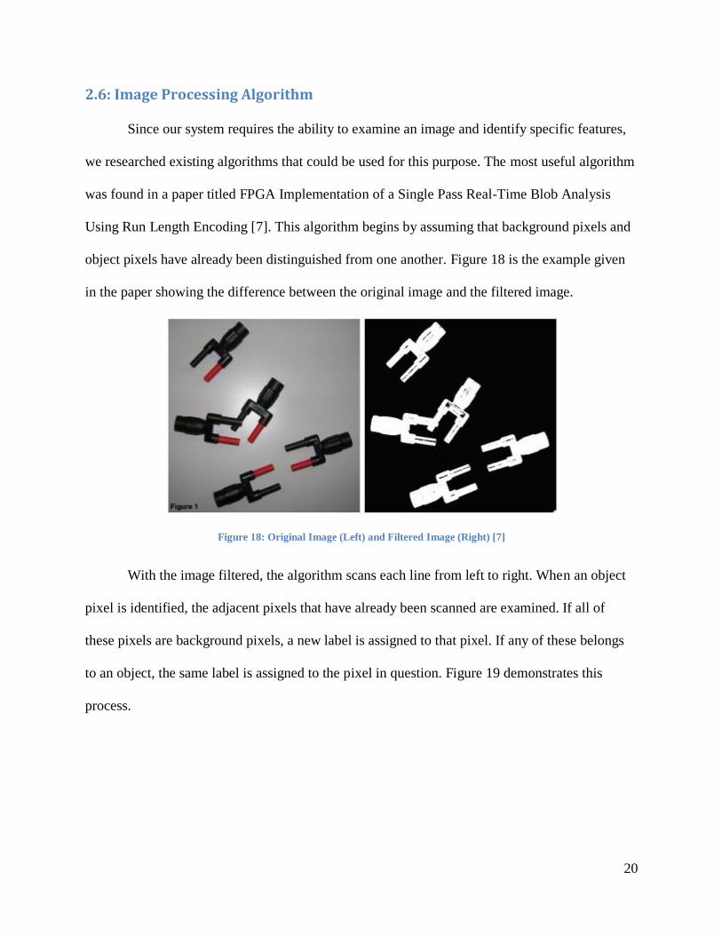
Since our system requires the ability to examine an image and identify specific features,
we researched existing algorithms that could be used for this purpose. The most useful algorithm
was found in a paper titled FPGA Implementation of a Single Pass Real-Time Blob Analysis
Using Run Length Encoding [7]. This algorithm begins by assuming that background pixels and
object pixels have already been distinguished from one another. Figure 18 is the example given
in the paper showing the difference between the original image and the filtered image.
Figure 18: Original Image (Left) and Filtered Image (Right) [7]
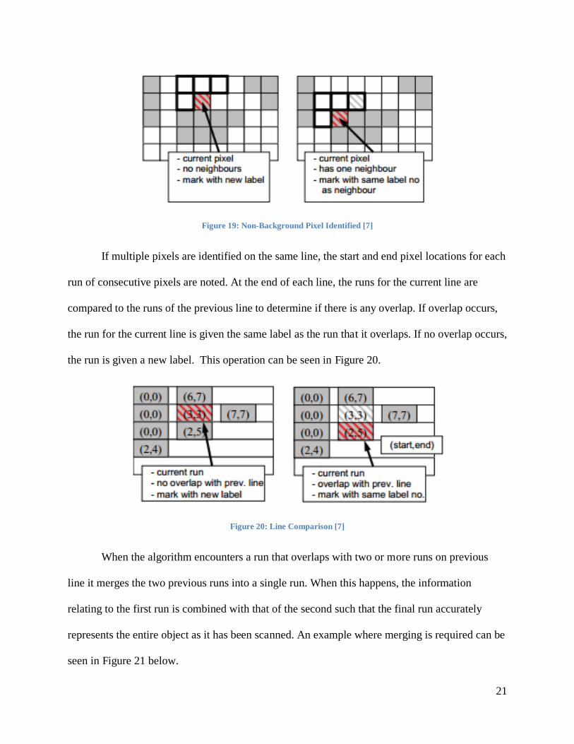
With the image filtered, the algorithm scans each line from left to right. When an object
pixel is identified, the adjacent pixels that have already been scanned are examined. If all of
these pixels are background pixels, a new label is assigned to that pixel. If any of these belongs
to an object, the same label is assigned to the pixel in question. Figure 19 demonstrates this
process.
21
Figure 19: Non-Background Pixel Identified [7]
If multiple pixels are identified on the same line, the start and end pixel locations for each
run of consecutive pixels are noted. At the end of each line, the runs for the current line are
compared to the runs of the previous line to determine if there is any overlap. If overlap occurs,
the run for the current line is given the same label as the run that it overlaps. If no overlap occurs,
the run is given a new label. This operation can be seen in Figure 20.
Figure 20: Line Comparison [7]
When the algorithm encounters a run that overlaps with two or more runs on previous
line it merges the two previous runs into a single run. When this happens, the information
relating to the first run is combined with that of the second such that the final run accurately
represents the entire object as it has been scanned. An example where merging is required can be
seen in Figure 21 below.
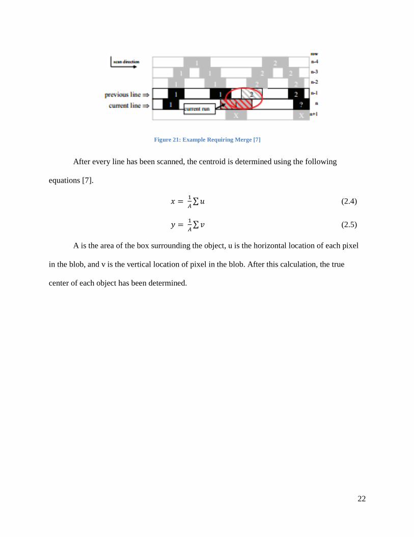
22
Figure 21: Example Requiring Merge [7]
After every line has been scanned, the centroid is determined using the following
equations [7].
(2.4)
(2.5)
A is the area of the box surrounding the object, u is the horizontal location of each pixel
in the blob, and v is the vertical location of pixel in the blob. After this calculation, the true
center of each object has been determined.
23
Chapter 3: System Design
From our background research, several issues were found that should be addressed. Our
system needs to be capable of tracking robots on an entire 27x54 foot field, that can have various
obstacles and ramps that can block sightlines and change the heights of robots. Also, since each
robot is independently controlled, each of the 6 robots playing the game should have a unique
visual ID that can be identified, independent of the robot’s design. Once images are captured, a
system must be developed to analyze the images to find the unique IDs. Then the perspective
distortion of the camera must be corrected, which allows accurate reconstruction of robot
locations.
The system that we designed to accomplish the goal of this project operates in four major
stages. The first stage of the system involves utilizing an array of LEDs to generate a specific
pattern of colors. The second stage is the image acquisition stage where images from the camera
are captured and stored. The third stage is the image processing stage where key data is extracted
from the images. The fourth and final stage is the reconstruction stage where data from multiple
cameras are combined to determine the locations of the robots.
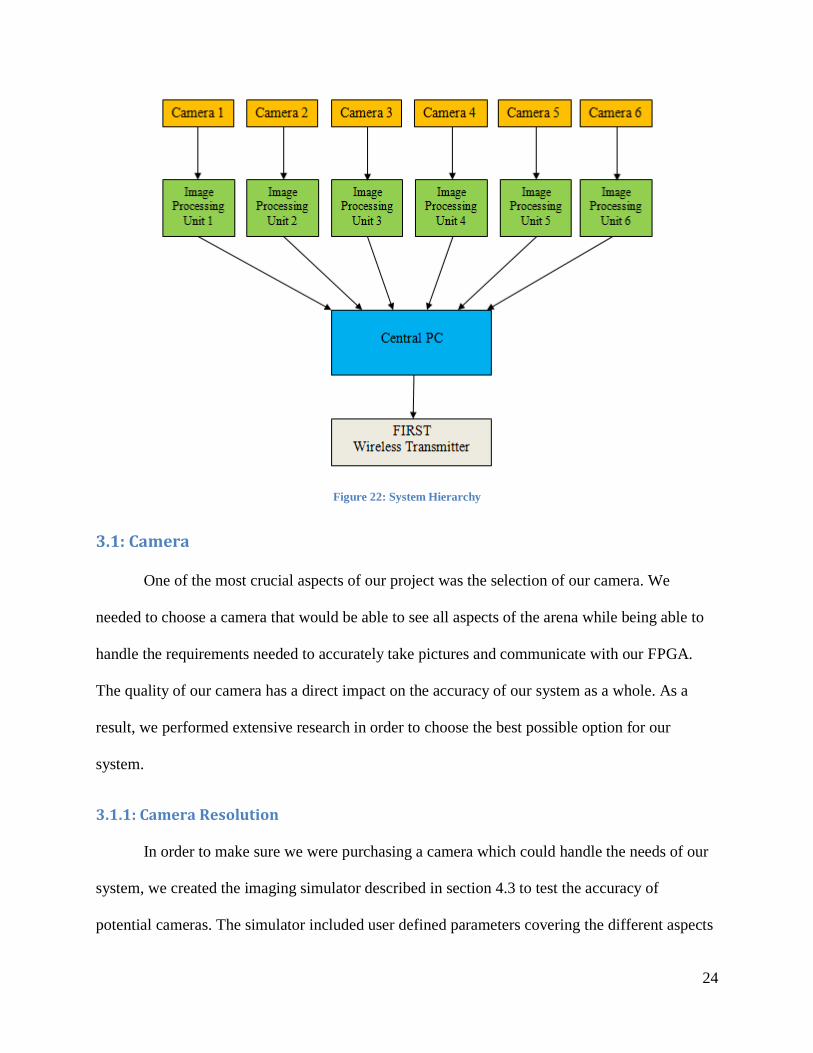
Figure 22 below shows the overall hierarchy for the full scale system. This system uses
six cameras placed around the arena. Each has its own FPGA embedded system to process the
images and send the results to the central PC. Once the data from the six cameras has been
received by the central PC, the locations of all of the robots are reconstructed and provided to
FIRST for distribution to the teams.
24
Figure 22: System Hierarchy
3.1: Camera
One of the most crucial aspects of our project was the selection of our camera. We
needed to choose a camera that would be able to see all aspects of the arena while being able to
handle the requirements needed to accurately take pictures and communicate with our FPGA.
The quality of our camera has a direct impact on the accuracy of our system as a whole. As a
result, we performed extensive research in order to choose the best possible option for our
system.
3.1.1: Camera Resolution
In order to make sure we were purchasing a camera which could handle the needs of our
system, we created the imaging simulator described in section 4.3 to test the accuracy of
potential cameras. The simulator included user defined parameters covering the different aspects
25
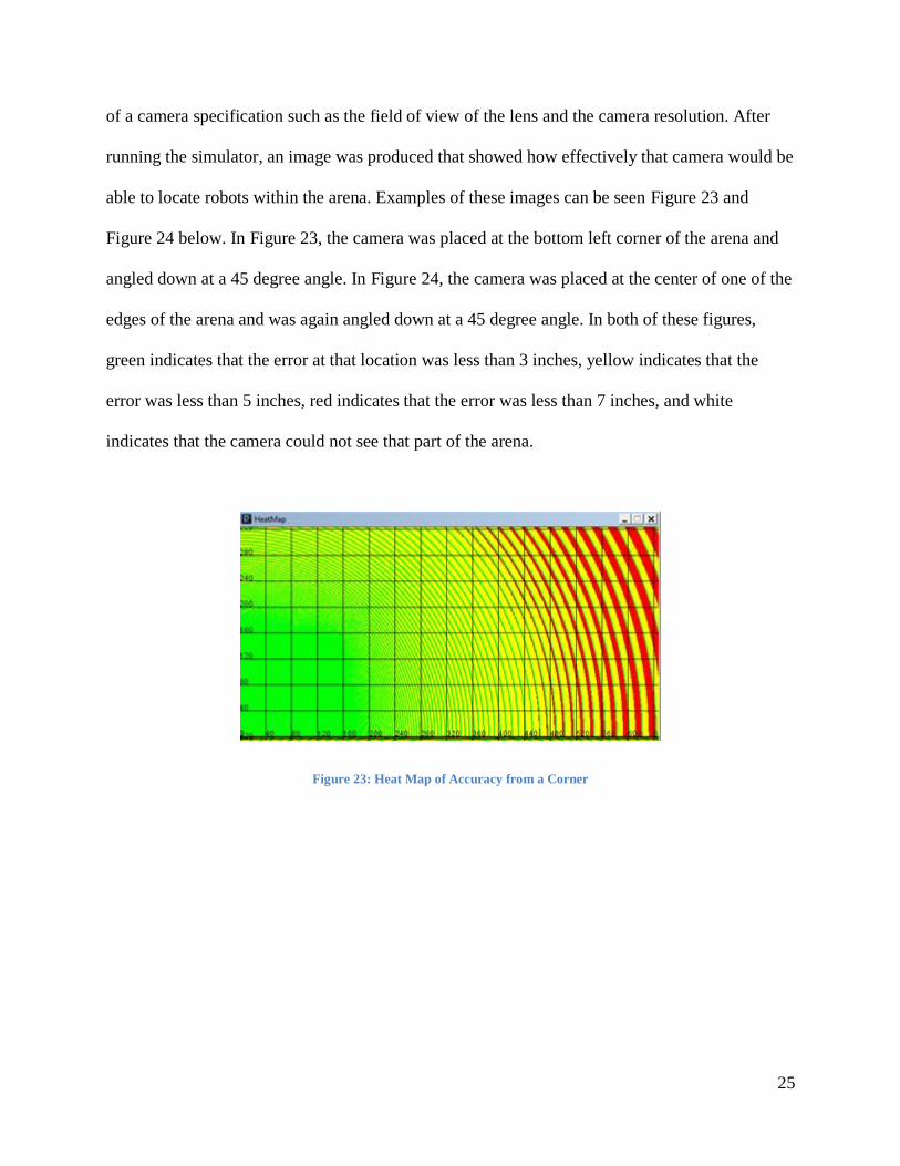
of a camera specification such as the field of view of the lens and the camera resolution. After
running the simulator, an image was produced that showed how effectively that camera would be
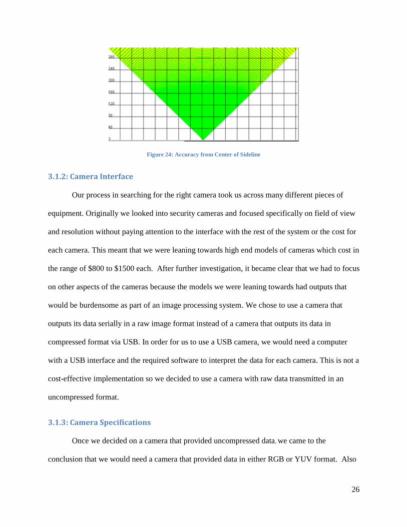
able to locate robots within the arena. Examples of these images can be seen Figure 23 and
Figure 24 below. In Figure 23, the camera was placed at the bottom left corner of the arena and
angled down at a 45 degree angle. In Figure 24, the camera was placed at the center of one of the
edges of the arena and was again angled down at a 45 degree angle. In both of these figures,
green indicates that the error at that location was less than 3 inches, yellow indicates that the
error was less than 5 inches, red indicates that the error was less than 7 inches, and white
indicates that the camera could not see that part of the arena.
Figure 23: Heat Map of Accuracy from a Corner
26
Figure 24: Accuracy from Center of Sideline
3.1.2: Camera Interface
Our process in searching for the right camera took us across many different pieces of
equipment. Originally we looked into security cameras and focused specifically on field of view
and resolution without paying attention to the interface with the rest of the system or the cost for
each camera. This meant that we were leaning towards high end models of cameras which cost in
the range of $800 to $1500 each. After further investigation, it became clear that we had to focus
on other aspects of the cameras because the models we were leaning towards had outputs that
would be burdensome as part of an image processing system. We chose to use a camera that
outputs its data serially in a raw image format instead of a camera that outputs its data in
compressed format via USB. In order for us to use a USB camera, we would need a computer
with a USB interface and the required software to interpret the data for each camera. This is not a
cost-effective implementation so we decided to use a camera with raw data transmitted in an
uncompressed format.
3.1.3: Camera Specifications
Once we decided on a camera that provided uncompressed data, we came to the
conclusion that we would need a camera that provided data in either RGB or YUV format. Also
27
on our list of specifications was a horizontal viewing angle of at least 95 degrees as well as an
86.5 degree vertical viewing angle to allow a 5 degree tolerance in either direction. These angles
would allow us to cover the field completely with enough overlap between the separate cameras
to ensure that the system would function with a high degree of accuracy. In looking at the camera
modules it became clear that we would be able to look for specifications such as resolution and
data output and leave the viewing angle issue for our choice of lens.
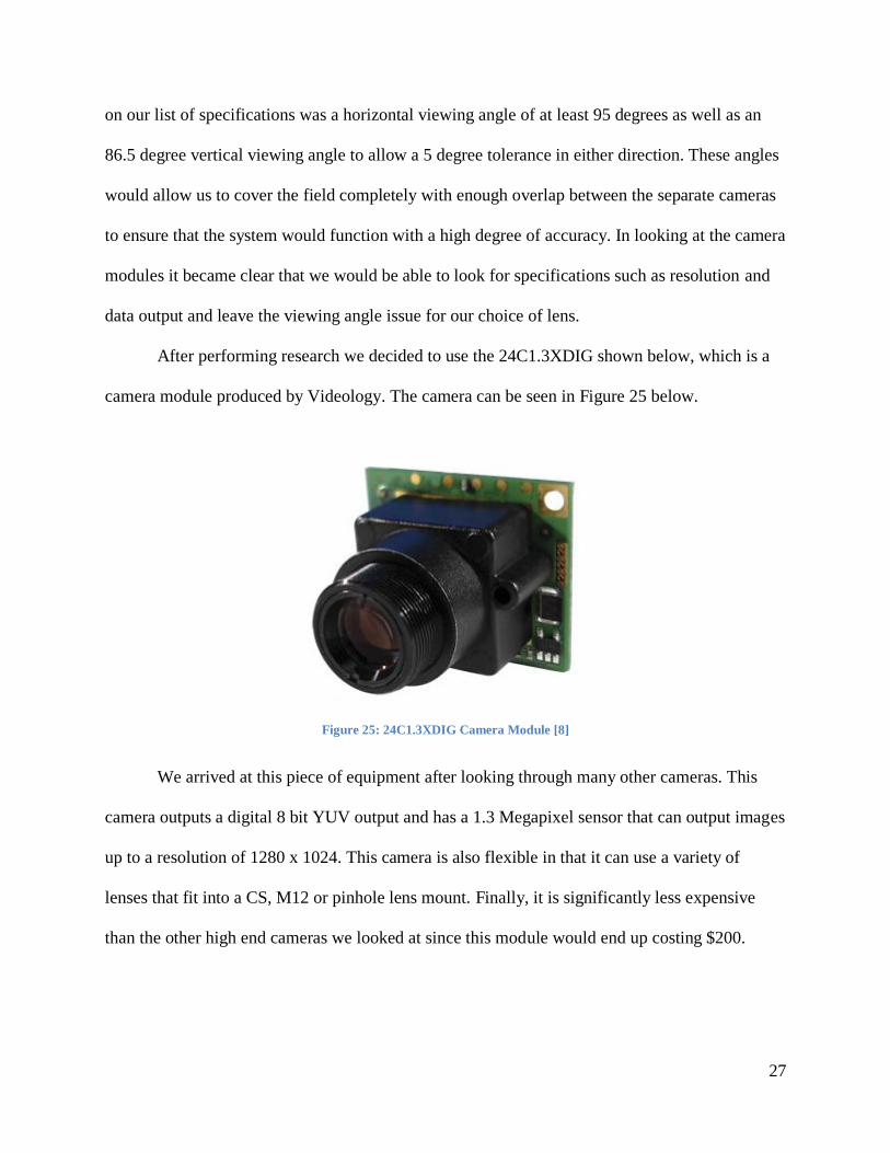
After performing research we decided to use the 24C1.3XDIG shown below, which is a
camera module produced by Videology. The camera can be seen in Figure 25 below.
Figure 25: 24C1.3XDIG Camera Module [8]
We arrived at this piece of equipment after looking through many other cameras. This
camera outputs a digital 8 bit YUV output and has a 1.3 Megapixel sensor that can output images
up to a resolution of 1280 x 1024. This camera is also flexible in that it can use a variety of
lenses that fit into a CS, M12 or pinhole lens mount. Finally, it is significantly less expensive
than the other high end cameras we looked at since this module would end up costing $200.
28
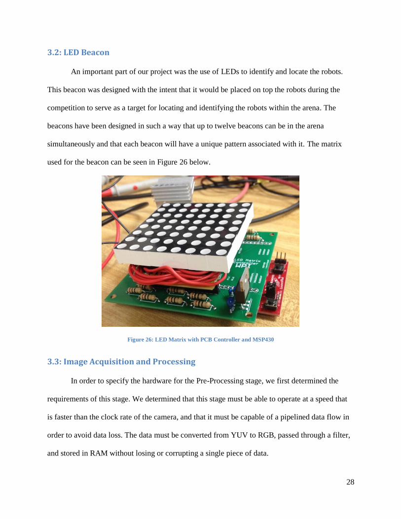
3.2: LED Beacon
An important part of our project was the use of LEDs to identify and locate the robots.
This beacon was designed with the intent that it would be placed on top the robots during the
competition to serve as a target for locating and identifying the robots within the arena. The
beacons have been designed in such a way that up to twelve beacons can be in the arena
simultaneously and that each beacon will have a unique pattern associated with it. The matrix
used for the beacon can be seen in Figure 26 below.
Figure 26: LED Matrix with PCB Controller and MSP430
3.3: Image Acquisition and Processing
In order to specify the hardware for the Pre-Processing stage, we first determined the
requirements of this stage. We determined that this stage must be able to operate at a speed that
is faster than the clock rate of the camera, and that it must be capable of a pipelined data flow in
order to avoid data loss. The data must be converted from YUV to RGB, passed through a filter,
and stored in RAM without losing or corrupting a single piece of data.
29
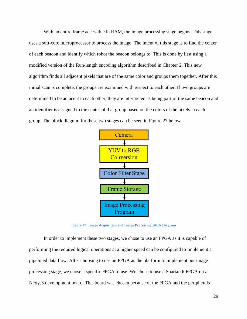
With an entire frame accessible in RAM, the image processing stage begins. This stage
uses a soft-core microprocessor to process the image. The intent of this stage is to find the center
of each beacon and identify which robot the beacon belongs to. This is done by first using a
modified version of the Run-length encoding algorithm described in Chapter 2. This new
algorithm finds all adjacent pixels that are of the same color and groups them together. After this
initial scan is complete, the groups are examined with respect to each other. If two groups are
determined to be adjacent to each other, they are interpreted as being part of the same beacon and
an identifier is assigned to the center of that group based on the colors of the pixels in each
group. The block diagram for these two stages can be seen in Figure 27 below.
Figure 27: Image Acquisition and Image Processing Block Diagram
In order to implement these two stages, we chose to use an FPGA as it is capable of
performing the required logical operations at a higher speed can be configured to implement a
pipelined data flow. After choosing to use an FPGA as the platform to implement our image
processing stage, we chose a specific FPGA to use. We chose to use a Spartan 6 FPGA on a
Nexys3 development board. This board was chosen because of the FPGA and the peripherals

30
such as the RAM as well as UART and VGA display ports it contains. This FPGA is capable of
operating at a speed significantly higher than the camera we chose and is large enough that it is
able to easily support our system design. The RAM peripheral on this board is necessary for
storing an image so that the entire image can be processed at the same time. With all of these
capabilities, the Spartan 6 FPGA on a Nexys3 development board was the best choice for
developing our Image Processing stage.
3.4: Beacon Location Reconstruction
Once each camera has finished processing a frame, it transmits the pixel coordinates of
the center of each beacon along with its identifier to a central computer. The final stage
reconciles data from multiple cameras in order to reconstruct the real world coordinates of the
beacons. The program that runs the user interface with the PC and performs the coordinate
reconstruction was made to be portable so any PC running Windows can run the program.
31
Chapter 4: Modules for Testing
4.1: Camera Model
Since many of the Verilog modules we developed relied on receiving data from the
camera, we developed a model of the camera. This model was designed in such a way that it
produced the same signals as the camera. These signals included 8 bits of image data, a signal
indicating when a horizontal line had ended, a signal indicating when a frame ended, and the 54
MHz clock that the camera provides. With this model successfully implemented, we were able to
test our digital logic models in simulation. By simulating these modules, we significantly
decreased the amount of time required to debug each system. This is because simulations provide
significantly more visibility of all of the signals in a module than testing on a physical FPGA
would.
4.2: VGA Display
In order to facilitate our testing, we designed a module that was capable of reading image
data from RAM and displaying it on a VGA display. This module has two main components.
The first component generates the timing signals required to communicate with the display. This
is done by using a 25 MHz clock which increments two counters. These two counters drive
synchronization signals which set the monitor to display an image at 640X480 resolution. The
second component utilizes a FIFO to ensure that color data is always available and accurate. This
is done by continuously writing pixel data from RAM until the FIFO is full. While data is being
written in, data is simultaneously read out to drive the VGA display. By doing this, the display
will always have pixel data ready when it is needed.
32
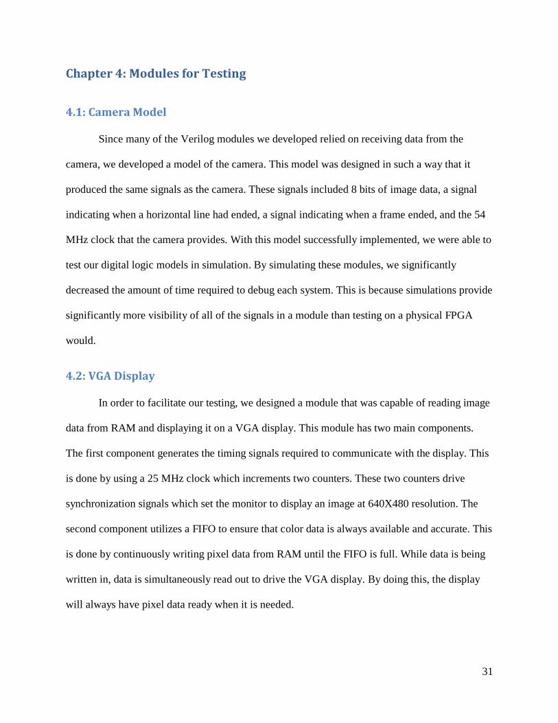
After implementing the VGA Display module, a testbench was created in order to verify
that data was available to send to the display at the proper times. The result of this test can be
seen in Figure 28 below. This figure particularly demonstrates that data is passed into the system
64 bits at a time and sent to the monitor 8 bits at a time. Additionally, the signal that indicates
that the FIFO cannot hold more data is shown.
Figure 28: VGA Display Testbench
4.3: Imaging Model
Since our project is based on using images to find object locations, it was very important
to develop an understanding for how three-dimensional locations are projected onto a two-
dimensional image plane. This was done by developing a model for the camera. Initially a
simple model was developed, but it was found to be too limited, and did not accurately represent
the camera. This motivated the development and implementation of a more complex imaging
model.
33
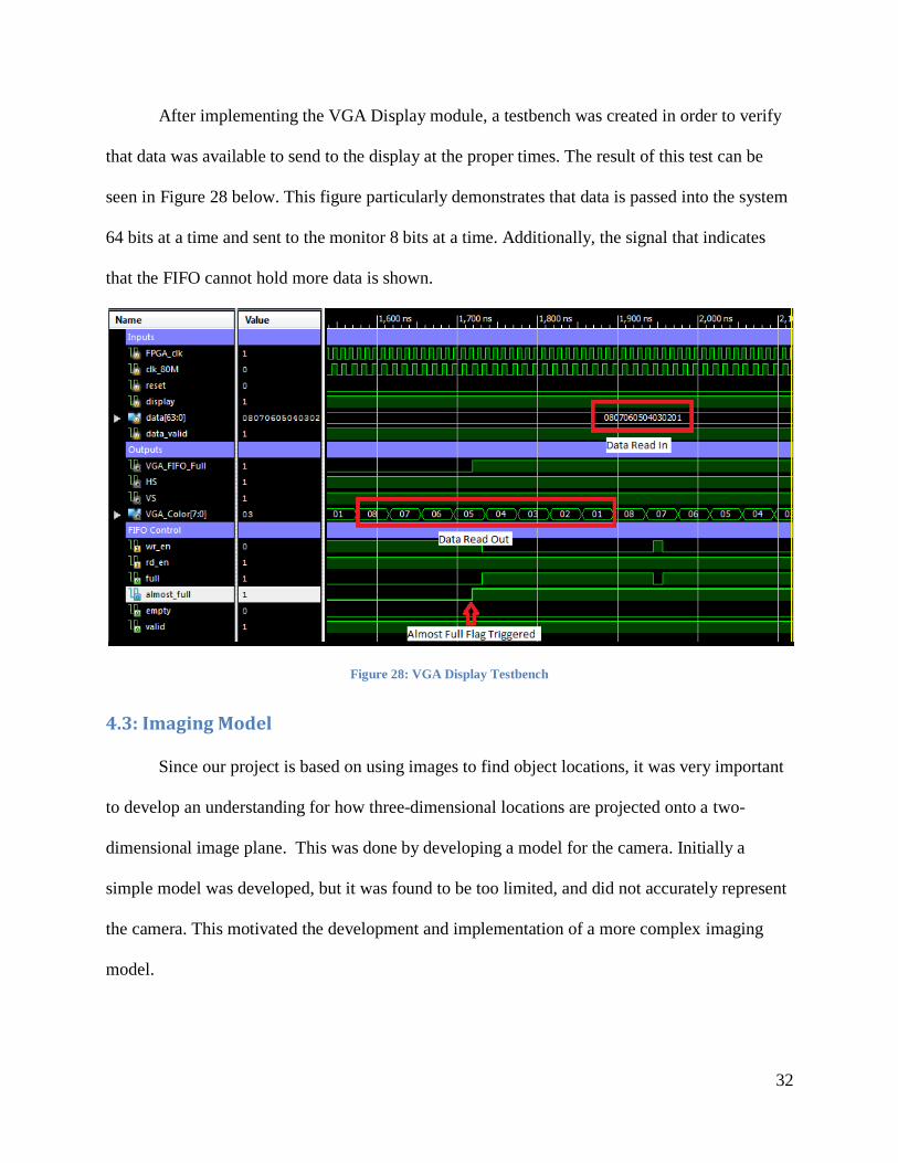
The initial model developed attempted to treat horizontal and vertical displacement in the
image as functions of single angles. Distance left or right from the center of the image was
assumed to be a function of a single angle because the object imaged was to the left or right of an
imaginary plane determined by the yaw angle of the camera as shown in Figure 29, and distance
up or down was assumed to be because the object was above or below a plane determined by the
pitch angle of the camera. This created an easy model to calculate, but we noticed it did not
properly simulate images of objects when implemented. For instance, Figure 29 shows a red and
green object being imaged by a camera located at the bottom left corner of the setup. Since the
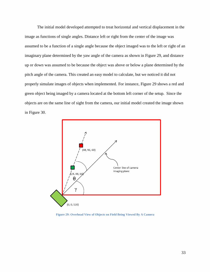
objects are on the same line of sight from the camera, our initial model created the image shown
in Figure 30.
Figure 29: Overhead View of Objects on Field Being Viewed By A Camera
34
Figure 30: Image of the Scene in Figure 29 Using Our Simple Camera Model
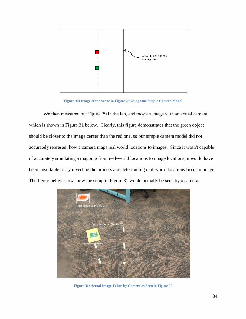
We then measured out Figure 29 in the lab, and took an image with an actual camera,
which is shown in Figure 31 below. Clearly, this figure demonstrates that the green object
should be closer to the image center than the red one, so our simple camera model did not
accurately represent how a camera maps real world locations to images. Since it wasn't capable
of accurately simulating a mapping from real-world locations to image locations, it would have
been unsuitable to try inverting the process and determining real-world locations from an image.
The figure below shows how the setup in Figure 31 would actually be seen by a camera.
Figure 31: Actual Image Taken by Camera as Seen in Figure 29
35
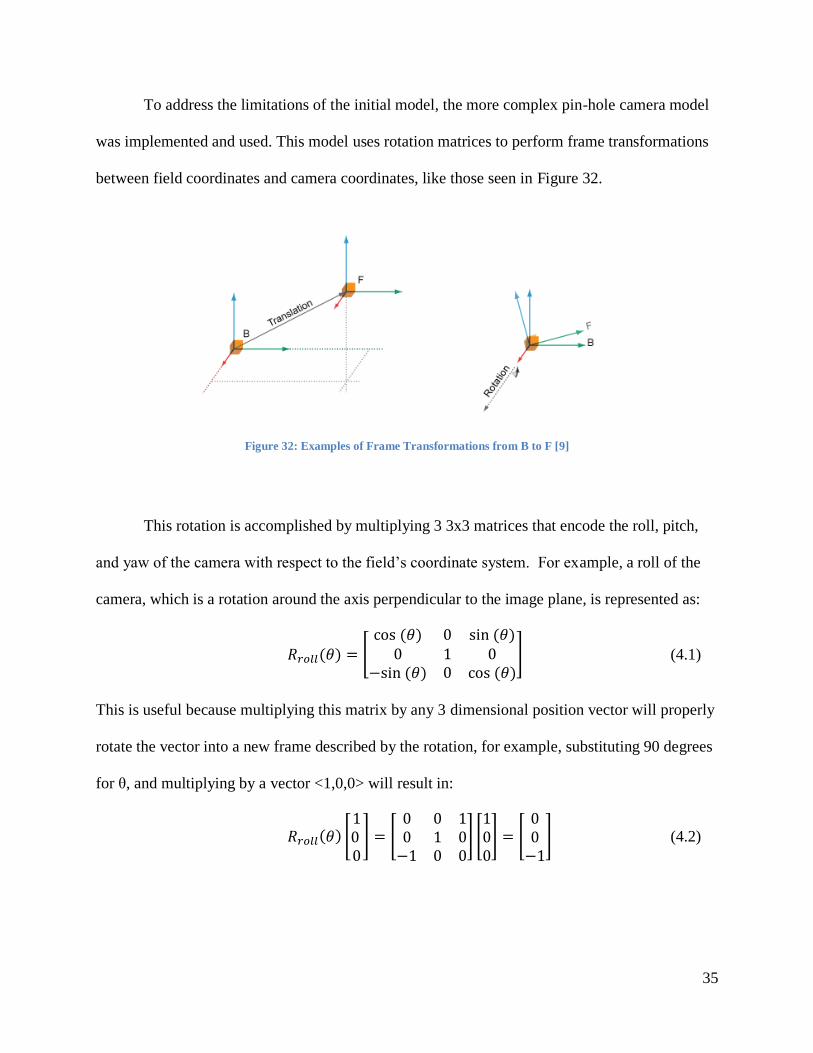
To address the limitations of the initial model, the more complex pin-hole camera model
was implemented and used. This model uses rotation matrices to perform frame transformations
between field coordinates and camera coordinates, like those seen in Figure 32.
Figure 32: Examples of Frame Transformations from B to F [9]
This rotation is accomplished by multiplying 3 3x3 matrices that encode the roll, pitch,
and yaw of the camera with respect to the field’s coordinate system. For example, a roll of the
camera, which is a rotation around the axis perpendicular to the image plane, is represented as:
(4.1)
This is useful because multiplying this matrix by any 3 dimensional position vector will properly
rotate the vector into a new frame described by the rotation, for example, substituting 90 degrees
for θ, and multiplying by a vector <1,0,0> will result in:
(4.2)
36
This indicates that a 90 degree roll is a transformation around the y-axis of the field. A single
simple rotation matrix like Rroll is a rotation around a single axis. By combining 3 of them, a full
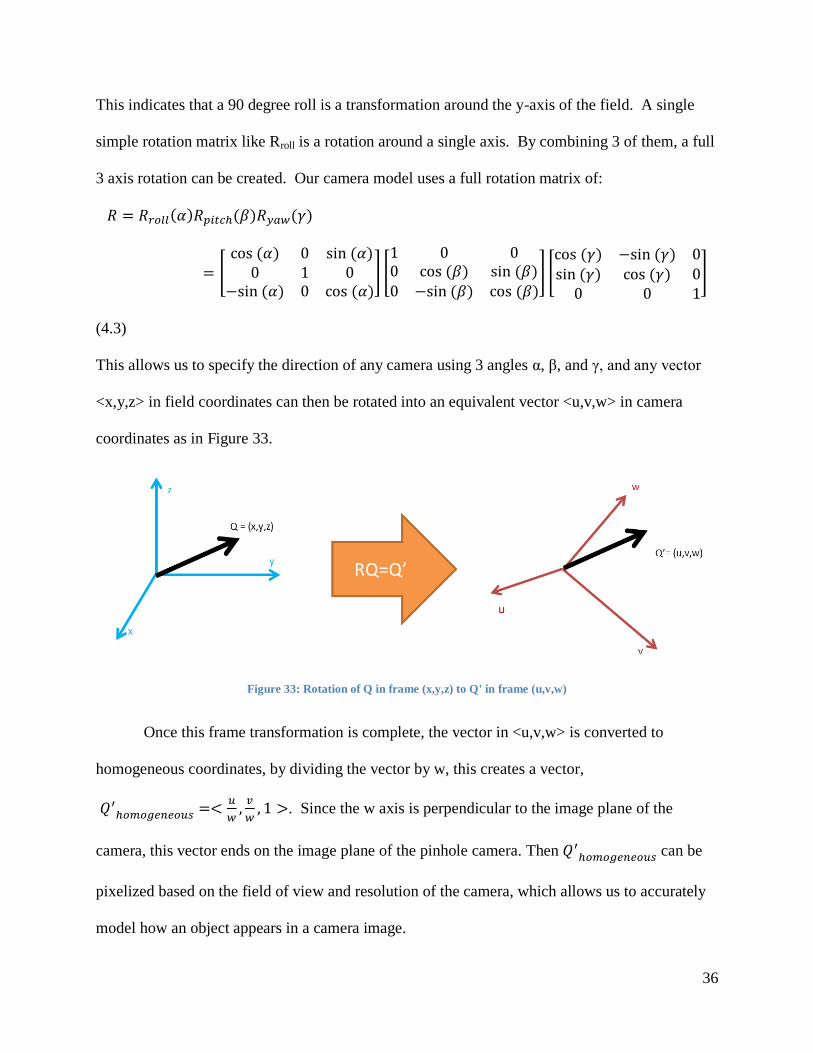
3 axis rotation can be created. Our camera model uses a full rotation matrix of:
(4.3)
This allows us to specify the direction of any camera using 3 angles α, β, and γ, and any vector
<x,y,z> in field coordinates can then be rotated into an equivalent vector <u,v,w> in camera
coordinates as in Figure 33.
Figure 33: Rotation of Q in frame (x,y,z) to Q' in frame (u,v,w)
Once this frame transformation is complete, the vector in <u,v,w> is converted to
homogeneous coordinates, by dividing the vector by w, this creates a vector,
. Since the w axis is perpendicular to the image plane of the
camera, this vector ends on the image plane of the pinhole camera. Then can be
pixelized based on the field of view and resolution of the camera, which allows us to accurately
model how an object appears in a camera image.
37
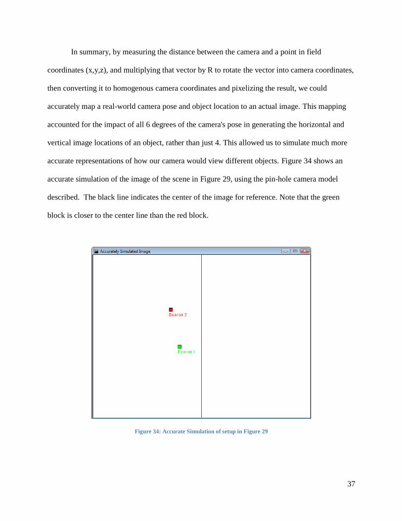
In summary, by measuring the distance between the camera and a point in field
coordinates (x,y,z), and multiplying that vector by R to rotate the vector into camera coordinates,
then converting it to homogenous camera coordinates and pixelizing the result, we could
accurately map a real-world camera pose and object location to an actual image. This mapping
accounted for the impact of all 6 degrees of the camera's pose in generating the horizontal and
vertical image locations of an object, rather than just 4. This allowed us to simulate much more
accurate representations of how our camera would view different objects. Figure 34 shows an
accurate simulation of the image of the scene in Figure 29, using the pin-hole camera model
described. The black line indicates the center of the image for reference. Note that the green
block is closer to the center line than the red block.
Figure 34: Accurate Simulation of setup in Figure 29

38
This imaging model was heavily used throughout project development. It helped us
determine how camera and lens parameters such as resolution and field of view impacted our
field coverage, which helped us develop our design specifications. It also helped quantify
beacon size and pattern resolution limitations. Finally, it was used directly to map images back
to 3 dimensional locations once the central PC received the image data from the FPGA.

39
Chapter 5: System Implementation
With testing modules successfully implemented, we were able to implement and test our
individual modules. This chapter describes the requirements, implementation process, and tests
performed for each module we developed.
5.1: Tracking Beacon
Our tracking beacon had to be designed and constructed in a manner that was efficient
and compatible with our camera system. This section describes how we designed and
implemented our beacon to meet this requirement.
5.1.1: Requirements
The requirements for our beacon were very straightforward. The first was that it had to be
clearly visible to our camera and able to be powered by the robots in the competition. Another
requirement was that there had to be the ability to display multiple patterns in order to uniquely
identify multiple robots within the arena. The final requirement of the tracking beacon was that
it had to be simple enough that people who worked the FIRST competition with no knowledge of
the system would be able to work our beacon design. Patterns for the beacon can be selected
simply by pushing a button.
5.1.2: Design Choices and Considerations
The beacon design evolved from many different ideas. We first came up a set of 3 LEDs
in a triangle for our beacon consisting of red, green or blue. This was because the front LED
could be used to help identify which robot was which due to the position of the 2 rear LEDs.
This allowed us to track up to 6 possible robots but lacked the ability to expand that number
should FIRST decide to add more robots to a playing field. Also in implementing the LEDs we
40
decided to use RGB tri-colored LEDs because they were easily identifiable, as well as being
easier to use because of the simplicity in changing the color of the LED when needed for beacon
patterns. The idea behind this method was to use trigonometry to determine a reference point’s
location as seen in Figure 35 below.
Figure 35: Original Beacon Layout
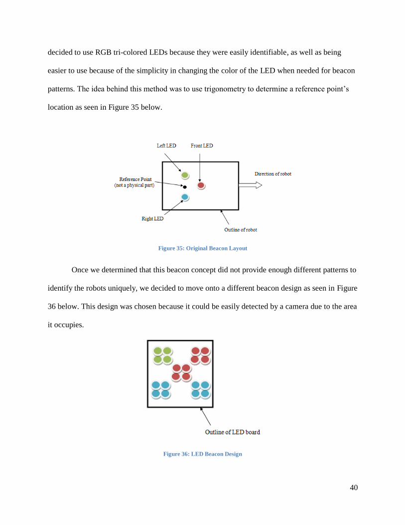
Once we determined that this beacon concept did not provide enough different patterns to
identify the robots uniquely, we decided to move onto a different beacon design as seen in Figure
36 below. This design was chosen because it could be easily detected by a camera due to the area
it occupies.
Figure 36: LED Beacon Design
41
However, after receiving and testing the LEDs in lab, we came to the conclusion that this
design was inefficient because it would require more space to implement and this would make
our design being more intrusive to the competitors.
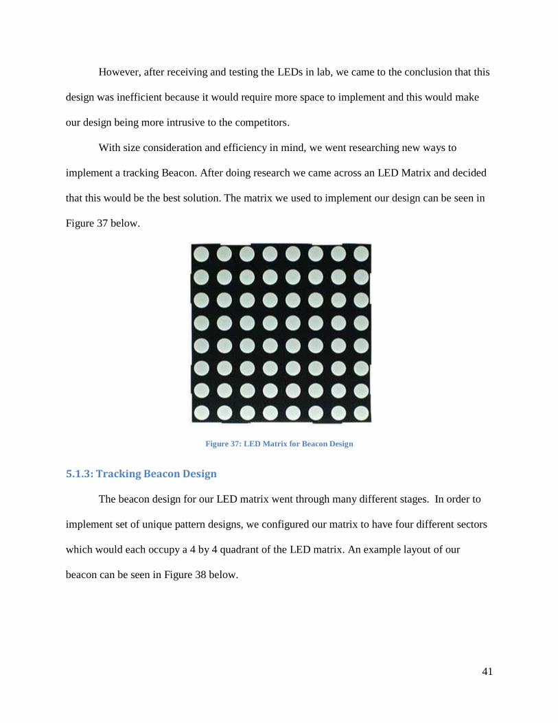
With size consideration and efficiency in mind, we went researching new ways to
implement a tracking Beacon. After doing research we came across an LED Matrix and decided
that this would be the best solution. The matrix we used to implement our design can be seen in
Figure 37 below.
Figure 37: LED Matrix for Beacon Design
5.1.3: Tracking Beacon Design
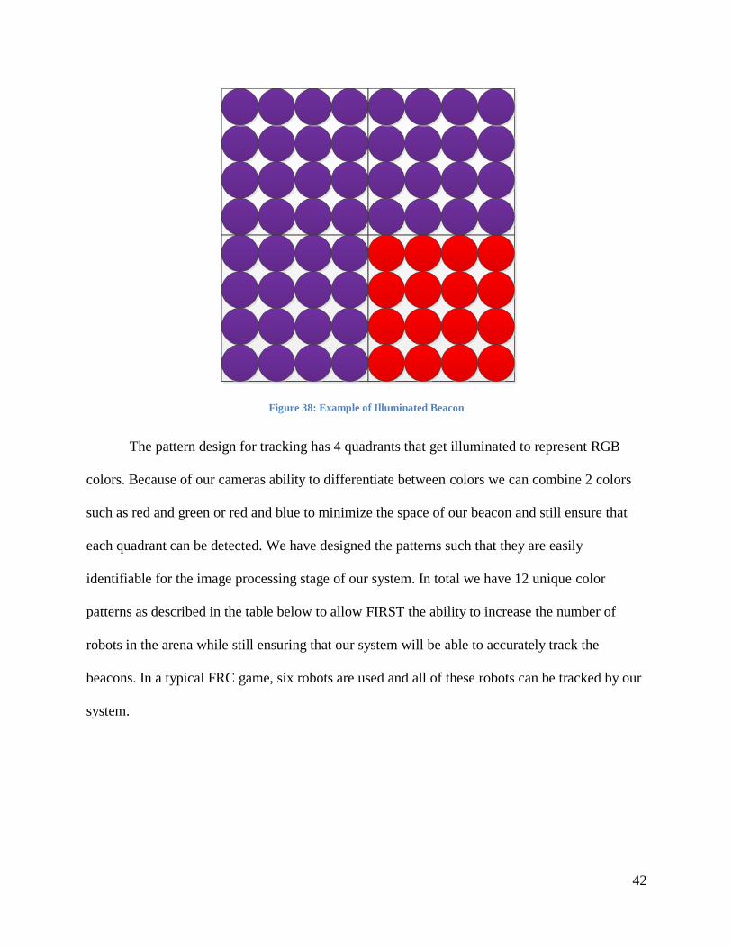
The beacon design for our LED matrix went through many different stages. In order to
implement set of unique pattern designs, we configured our matrix to have four different sectors
which would each occupy a 4 by 4 quadrant of the LED matrix. An example layout of our
beacon can be seen in Figure 38 below.
42
Figure 38: Example of Illuminated Beacon
The pattern design for tracking has 4 quadrants that get illuminated to represent RGB
colors. Because of our cameras ability to differentiate between colors we can combine 2 colors
such as red and green or red and blue to minimize the space of our beacon and still ensure that
each quadrant can be detected. We have designed the patterns such that they are easily
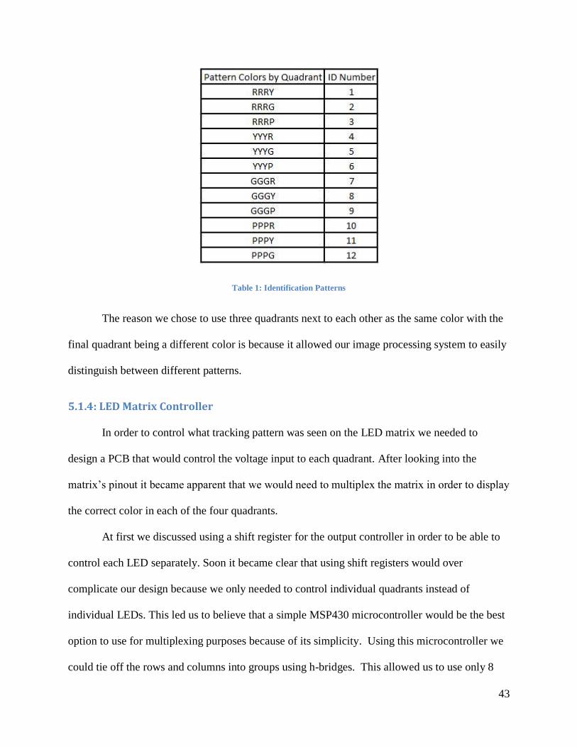
identifiable for the image processing stage of our system. In total we have 12 unique color
patterns as described in the table below to allow FIRST the ability to increase the number of
robots in the arena while still ensuring that our system will be able to accurately track the
beacons. In a typical FRC game, six robots are used and all of these robots can be tracked by our
system.
43
Table 1: Identification Patterns
The reason we chose to use three quadrants next to each other as the same color with the
final quadrant being a different color is because it allowed our image processing system to easily
distinguish between different patterns.
5.1.4: LED Matrix Controller
In order to control what tracking pattern was seen on the LED matrix we needed to
design a PCB that would control the voltage input to each quadrant. After looking into the
matrix’s pinout it became apparent that we would need to multiplex the matrix in order to display
the correct color in each of the four quadrants.
At first we discussed using a shift register for the output controller in order to be able to
control each LED separately. Soon it became clear that using shift registers would over
complicate our design because we only needed to control individual quadrants instead of
individual LEDs. This led us to believe that a simple MSP430 microcontroller would be the best
option to use for multiplexing purposes because of its simplicity. Using this microcontroller we
could tie off the rows and columns into groups using h-bridges. This allowed us to use only 8
44
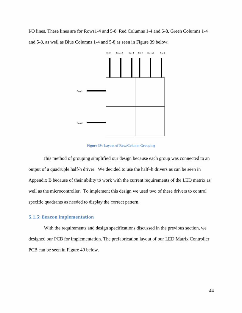
I/O lines. These lines are for Rows1-4 and 5-8, Red Columns 1-4 and 5-8, Green Columns 1-4
and 5-8, as well as Blue Columns 1-4 and 5-8 as seen in Figure 39 below.
Figure 39: Layout of Row/Column Grouping
This method of grouping simplified our design because each group was connected to an
output of a quadruple half-h driver. We decided to use the half–h drivers as can be seen in
Appendix B because of their ability to work with the current requirements of the LED matrix as
well as the microcontroller. To implement this design we used two of these drivers to control
specific quadrants as needed to display the correct pattern.
5.1.5: Beacon Implementation
With the requirements and design specifications discussed in the previous section, we
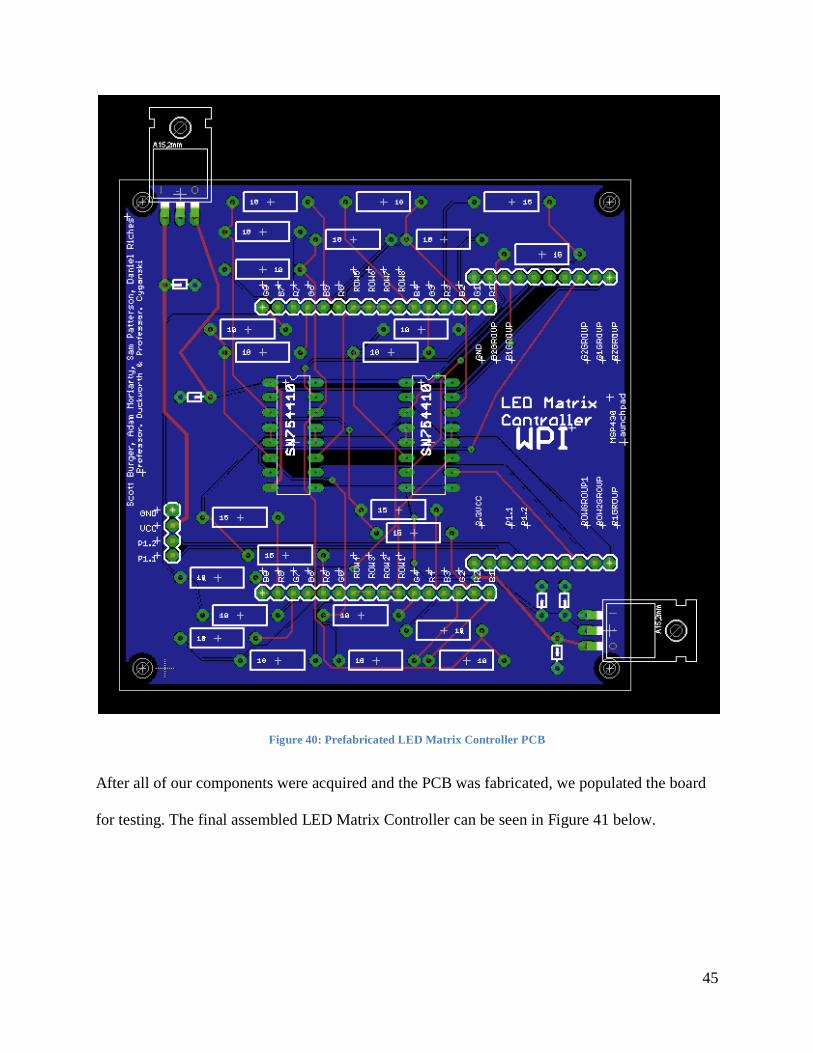
designed our PCB for implementation. The prefabrication layout of our LED Matrix Controller
PCB can be seen in Figure 40 below.
45
Figure 40: Prefabricated LED Matrix Controller PCB
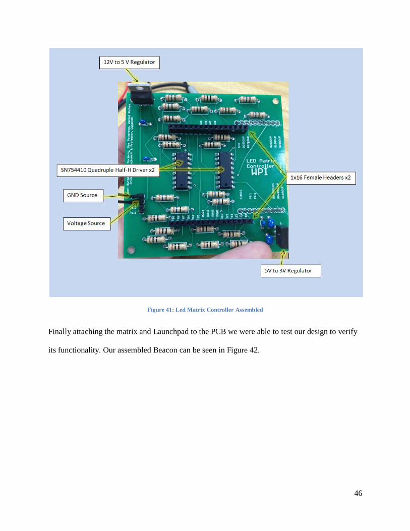
After all of our components were acquired and the PCB was fabricated, we populated the board
for testing. The final assembled LED Matrix Controller can be seen in Figure 41 below.
46
Figure 41: Led Matrix Controller Assembled
Finally attaching the matrix and Launchpad to the PCB we were able to test our design to verify
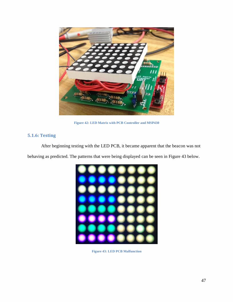
its functionality. Our assembled Beacon can be seen in Figure 42.
47
Figure 42: LED Matrix with PCB Controller and MSP430
5.1.6: Testing
After beginning testing with the LED PCB, it became apparent that the beacon was not
behaving as predicted. The patterns that were being displayed can be seen in Figure 43 below.
Figure 43: LED PCB Malfunction
48
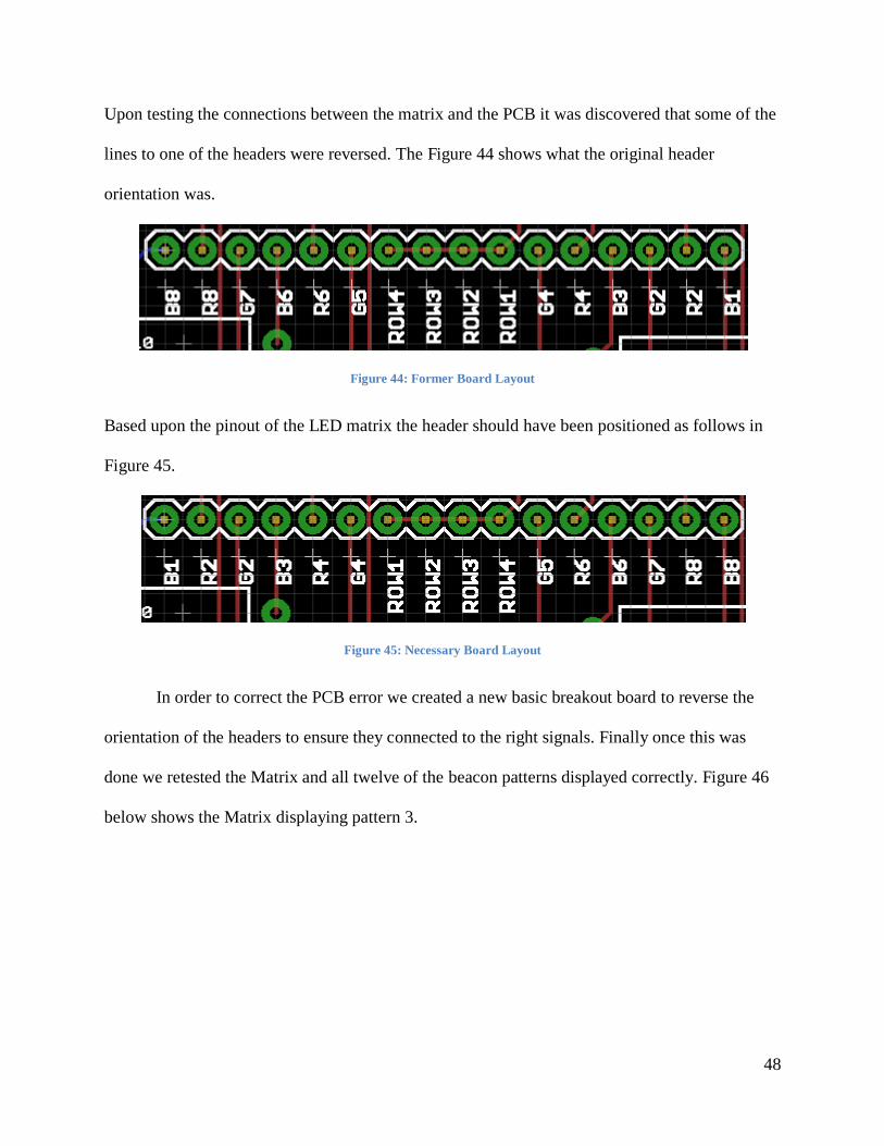
Upon testing the connections between the matrix and the PCB it was discovered that some of the
lines to one of the headers were reversed. The Figure 44 shows what the original header
orientation was.
Figure 44: Former Board Layout
Based upon the pinout of the LED matrix the header should have been positioned as follows in
Figure 45.
Figure 45: Necessary Board Layout
In order to correct the PCB error we created a new basic breakout board to reverse the
orientation of the headers to ensure they connected to the right signals. Finally once this was
done we retested the Matrix and all twelve of the beacon patterns displayed correctly. Figure 46
below shows the Matrix displaying pattern 3.
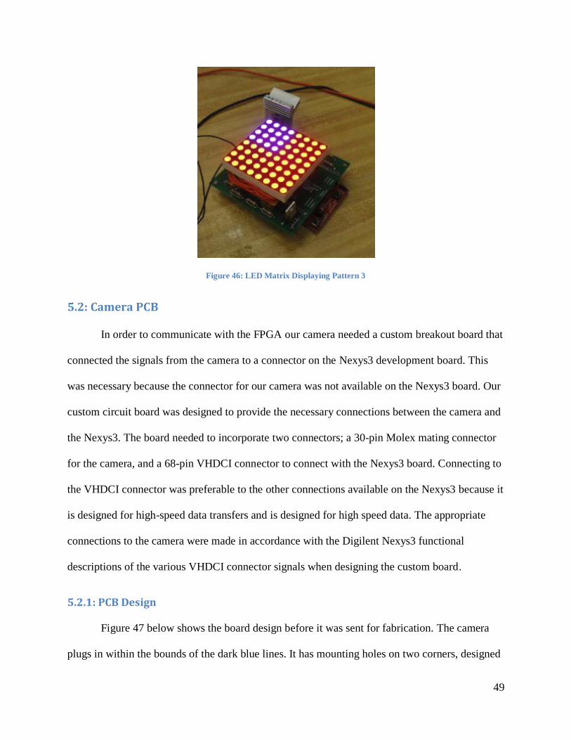
49
Figure 46: LED Matrix Displaying Pattern 3
5.2: Camera PCB
In order to communicate with the FPGA our camera needed a custom breakout board that
connected the signals from the camera to a connector on the Nexys3 development board. This
was necessary because the connector for our camera was not available on the Nexys3 board. Our
custom circuit board was designed to provide the necessary connections between the camera and
the Nexys3. The board needed to incorporate two connectors; a 30-pin Molex mating connector
for the camera, and a 68-pin VHDCI connector to connect with the Nexys3 board. Connecting to
the VHDCI connector was preferable to the other connections available on the Nexys3 because it
is designed for high-speed data transfers and is designed for high speed data. The appropriate
connections to the camera were made in accordance with the Digilent Nexys3 functional
descriptions of the various VHDCI connector signals when designing the custom board.
5.2.1: PCB Design
Figure 47 below shows the board design before it was sent for fabrication. The camera
plugs in within the bounds of the dark blue lines. It has mounting holes on two corners, designed
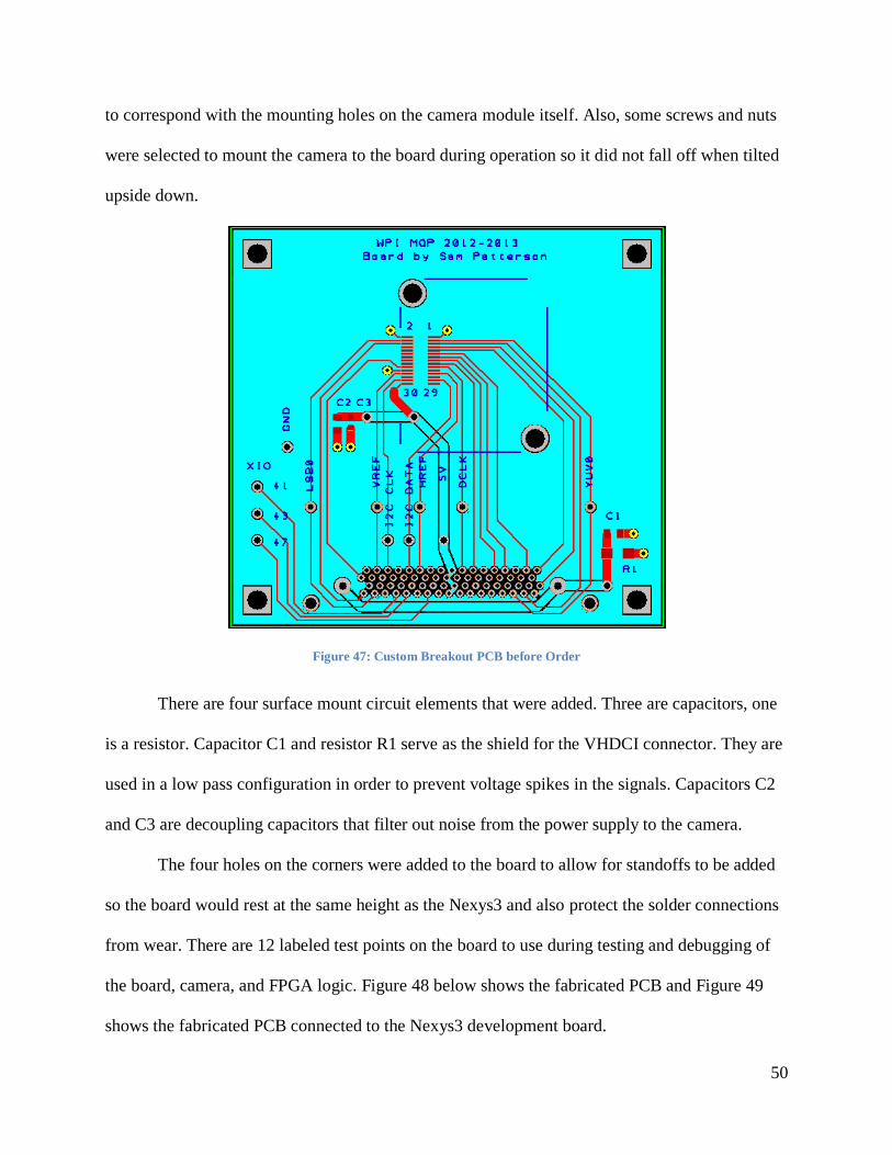
50
to correspond with the mounting holes on the camera module itself. Also, some screws and nuts
were selected to mount the camera to the board during operation so it did not fall off when tilted
upside down.
Figure 47: Custom Breakout PCB before Order
There are four surface mount circuit elements that were added. Three are capacitors, one
is a resistor. Capacitor C1 and resistor R1 serve as the shield for the VHDCI connector. They are
used in a low pass configuration in order to prevent voltage spikes in the signals. Capacitors C2
and C3 are decoupling capacitors that filter out noise from the power supply to the camera.
The four holes on the corners were added to the board to allow for standoffs to be added
so the board would rest at the same height as the Nexys3 and also protect the solder connections
from wear. There are 12 labeled test points on the board to use during testing and debugging of
the board, camera, and FPGA logic. Figure 48 below shows the fabricated PCB and Figure 49
shows the fabricated PCB connected to the Nexys3 development board.
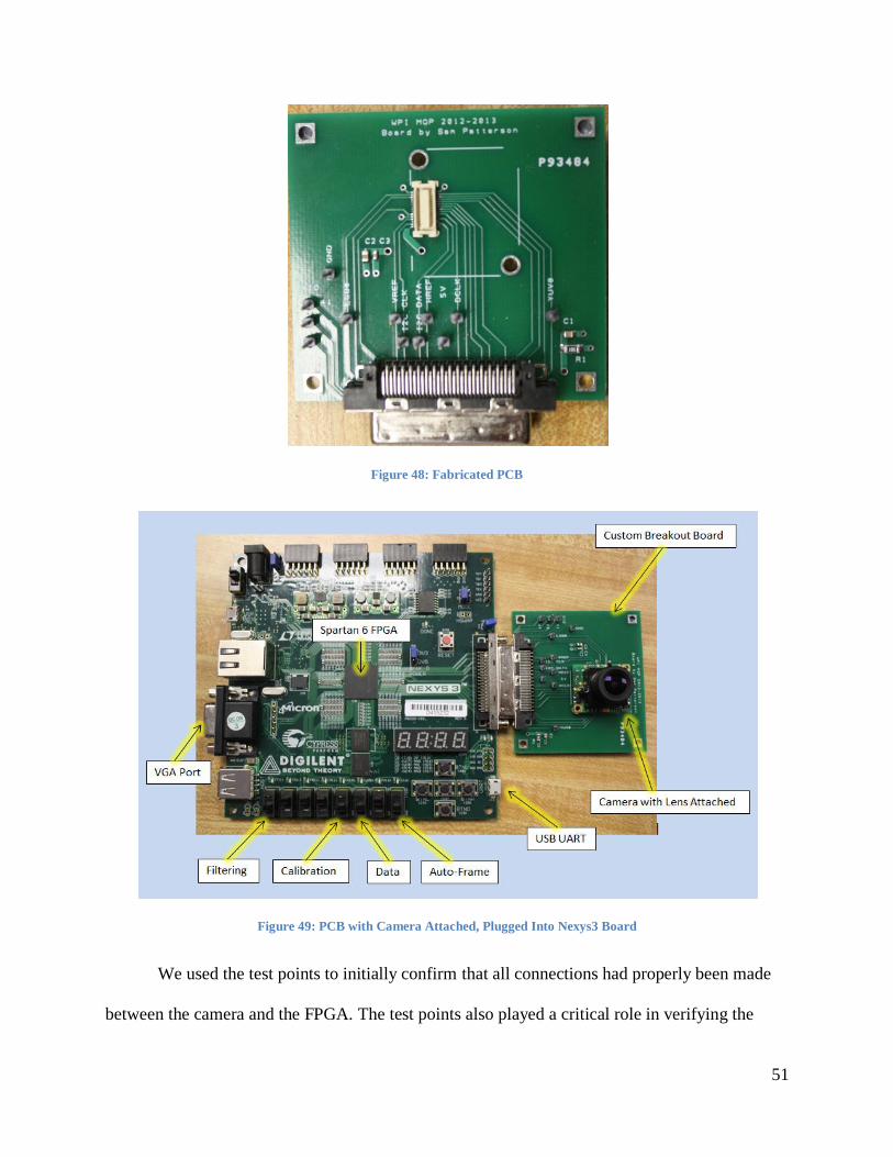
51
Figure 48: Fabricated PCB
Figure 49: PCB with Camera Attached, Plugged Into Nexys3 Board
We used the test points to initially confirm that all connections had properly been made
between the camera and the FPGA. The test points also played a critical role in verifying the
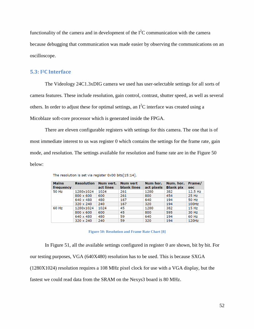
52
functionality of the camera and in development of the I2C communication with the camera
because debugging that communication was made easier by observing the communications on an
oscilloscope.
5.3: I2C Interface
The Videology 24C1.3xDIG camera we used has user-selectable settings for all sorts of
camera features. These include resolution, gain control, contrast, shutter speed, as well as several
others. In order to adjust these for optimal settings, an I2C interface was created using a
Micoblaze soft-core processor which is generated inside the FPGA.
There are eleven configurable registers with settings for this camera. The one that is of
most immediate interest to us was register 0 which contains the settings for the frame rate, gain
mode, and resolution. The settings available for resolution and frame rate are in the Figure 50
below:
Figure 50: Resolution and Frame Rate Chart [8]
In Figure 51, all the available settings configured in register 0 are shown, bit by bit. For
our testing purposes, VGA (640X480) resolution has to be used. This is because SXGA
(1280X1024) resolution requires a 108 MHz pixel clock for use with a VGA display, but the
fastest we could read data from the SRAM on the Nexys3 board is 80 MHz.
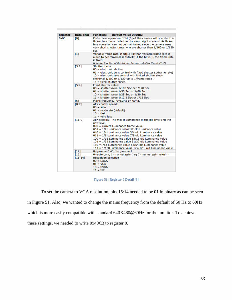
53
Figure 51: Register 0 Detail [8]
To set the camera to VGA resolution, bits 15:14 needed to be 01 in binary as can be seen
in Figure 51. Also, we wanted to change the mains frequency from the default of 50 Hz to 60Hz
which is more easily compatible with standard 640X480@60Hz for the monitor. To achieve
these settings, we needed to write 0x40C3 to register 0.
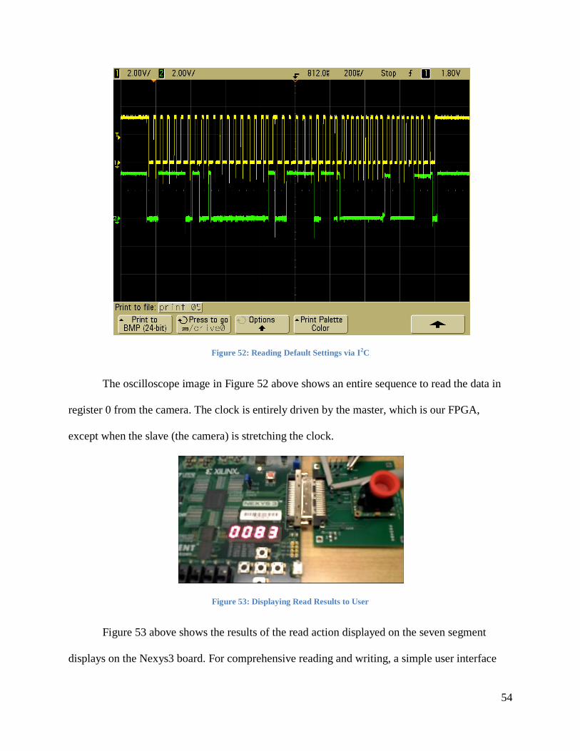
54
Figure 52: Reading Default Settings via I2C
The oscilloscope image in Figure 52 above shows an entire sequence to read the data in
register 0 from the camera. The clock is entirely driven by the master, which is our FPGA,
except when the slave (the camera) is stretching the clock.
Figure 53: Displaying Read Results to User
Figure 53 above shows the results of the read action displayed on the seven segment
displays on the Nexys3 board. For comprehensive reading and writing, a simple user interface
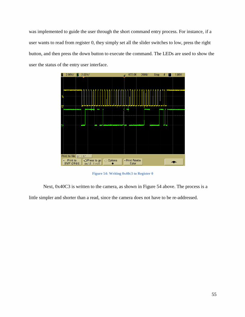
55
was implemented to guide the user through the short command entry process. For instance, if a
user wants to read from register 0, they simply set all the slider switches to low, press the right
button, and then press the down button to execute the command. The LEDs are used to show the
user the status of the entry user interface.
Figure 54: Writing 0x40c3 to Register 0
Next, 0x40C3 is written to the camera, as shown in Figure 54 above. The process is a
little simpler and shorter than a read, since the camera does not have to be re-addressed.
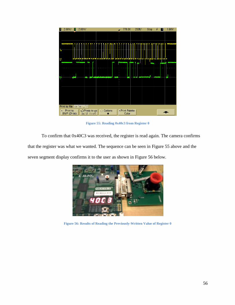
56
Figure 55: Reading 0x40c3 from Register 0
To confirm that 0x40C3 was received, the register is read again. The camera confirms
that the register was what we wanted. The sequence can be seen in Figure 55 above and the
seven segment display confirms it to the user as shown in Figure 56 below.
Figure 56: Results of Reading the Previously-Written Value of Register 0
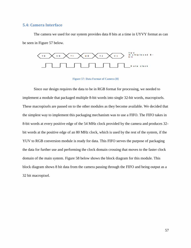
57
5.4: Camera Interface
The camera we used for our system provides data 8 bits at a time in UYVY format as can
be seen in Figure 57 below.
Figure 57: Data Format of Camera [8]
Since our design requires the data to be in RGB format for processing, we needed to
implement a module that packaged multiple 8-bit words into single 32-bit words, macropixels.
These macropixels are passed on to the other modules as they become available. We decided that
the simplest way to implement this packaging mechanism was to use a FIFO. The FIFO takes in
8-bit words at every positive edge of the 54 MHz clock provided by the camera and produces 32-
bit words at the positive edge of an 80 MHz clock, which is used by the rest of the system, if the
YUV to RGB conversion module is ready for data. This FIFO serves the purpose of packaging
the data for further use and performing the clock domain crossing that moves to the faster clock
domain of the main system. Figure 58 below shows the block diagram for this module. This
block diagram shows 8 bit data from the camera passing through the FIFO and being output as a
32 bit macropixel.
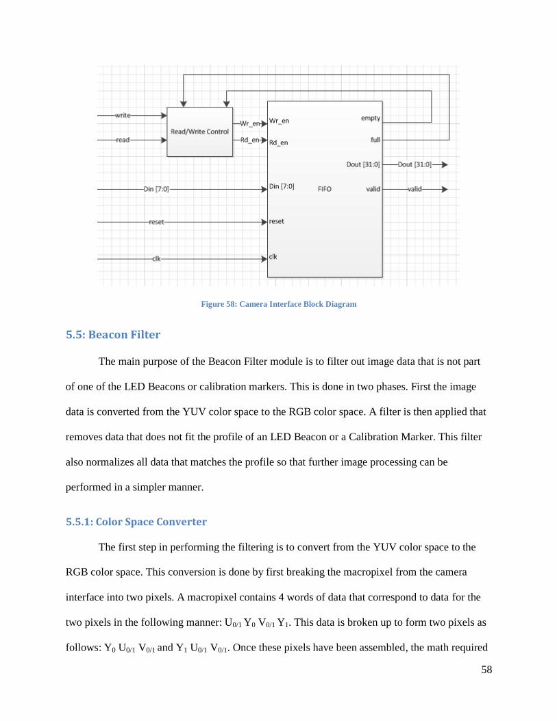
58
Figure 58: Camera Interface Block Diagram
5.5: Beacon Filter
The main purpose of the Beacon Filter module is to filter out image data that is not part
of one of the LED Beacons or calibration markers. This is done in two phases. First the image
data is converted from the YUV color space to the RGB color space. A filter is then applied that
removes data that does not fit the profile of an LED Beacon or a Calibration Marker. This filter
also normalizes all data that matches the profile so that further image processing can be
performed in a simpler manner.
5.5.1: Color Space Converter
The first step in performing the filtering is to convert from the YUV color space to the
RGB color space. This conversion is done by first breaking the macropixel from the camera
interface into two pixels. A macropixel contains 4 words of data that correspond to data for the
two pixels in the following manner: U0/1 Y0 V0/1 Y1. This data is broken up to form two pixels as
follows: Y0 U0/1 V0/1 and Y1 U0/1 V0/1. Once these pixels have been assembled, the math required
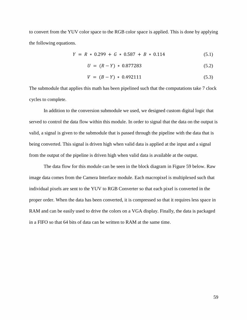
59
to convert from the YUV color space to the RGB color space is applied. This is done by applying
the following equations.
(5.1)
(5.2)
(5.3)
The submodule that applies this math has been pipelined such that the computations take 7 clock
cycles to complete.
In addition to the conversion submodule we used, we designed custom digital logic that
served to control the data flow within this module. In order to signal that the data on the output is
valid, a signal is given to the submodule that is passed through the pipeline with the data that is
being converted. This signal is driven high when valid data is applied at the input and a signal
from the output of the pipeline is driven high when valid data is available at the output.
The data flow for this module can be seen in the block diagram in Figure 59 below. Raw
image data comes from the Camera Interface module. Each macropixel is multiplexed such that
individual pixels are sent to the YUV to RGB Converter so that each pixel is converted in the
proper order. When the data has been converted, it is compressed so that it requires less space in
RAM and can be easily used to drive the colors on a VGA display. Finally, the data is packaged
in a FIFO so that 64 bits of data can be written to RAM at the same time.
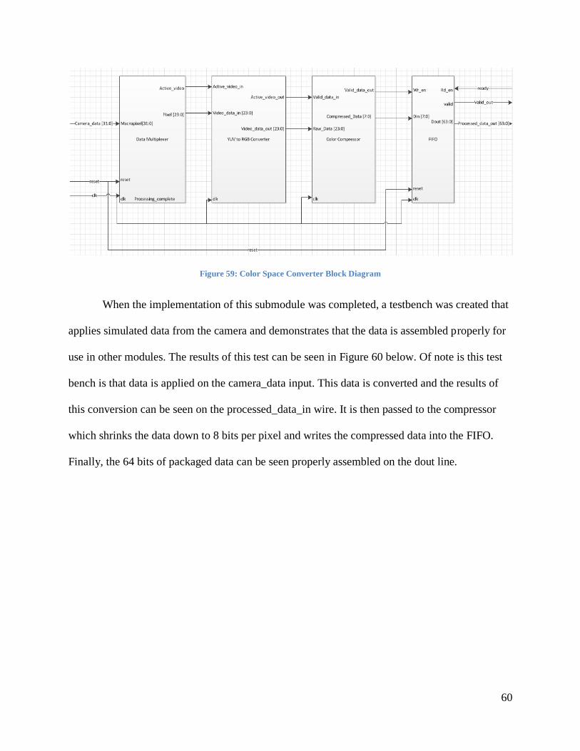
60
Figure 59: Color Space Converter Block Diagram
When the implementation of this submodule was completed, a testbench was created that
applies simulated data from the camera and demonstrates that the data is assembled properly for
use in other modules. The results of this test can be seen in Figure 60 below. Of note is this test
bench is that data is applied on the camera_data input. This data is converted and the results of
this conversion can be seen on the processed_data_in wire. It is then passed to the compressor
which shrinks the data down to 8 bits per pixel and writes the compressed data into the FIFO.
Finally, the 64 bits of packaged data can be seen properly assembled on the dout line.
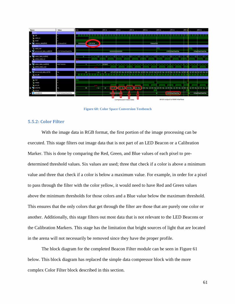
61
Figure 60: Color Space Conversion Testbench
5.5.2: Color Filter
With the image data in RGB format, the first portion of the image processing can be
executed. This stage filters out image data that is not part of an LED Beacon or a Calibration
Marker. This is done by comparing the Red, Green, and Blue values of each pixel to pre-
determined threshold values. Six values are used; three that check if a color is above a minimum
value and three that check if a color is below a maximum value. For example, in order for a pixel
to pass through the filter with the color yellow, it would need to have Red and Green values
above the minimum thresholds for those colors and a Blue value below the maximum threshold.
This ensures that the only colors that get through the filter are those that are purely one color or
another. Additionally, this stage filters out most data that is not relevant to the LED Beacons or
the Calibration Markers. This stage has the limitation that bright sources of light that are located
in the arena will not necessarily be removed since they have the proper profile.
The block diagram for the completed Beacon Filter module can be seen in Figure 61
below. This block diagram has replaced the simple data compressor block with the more
complex Color Filter block described in this section.
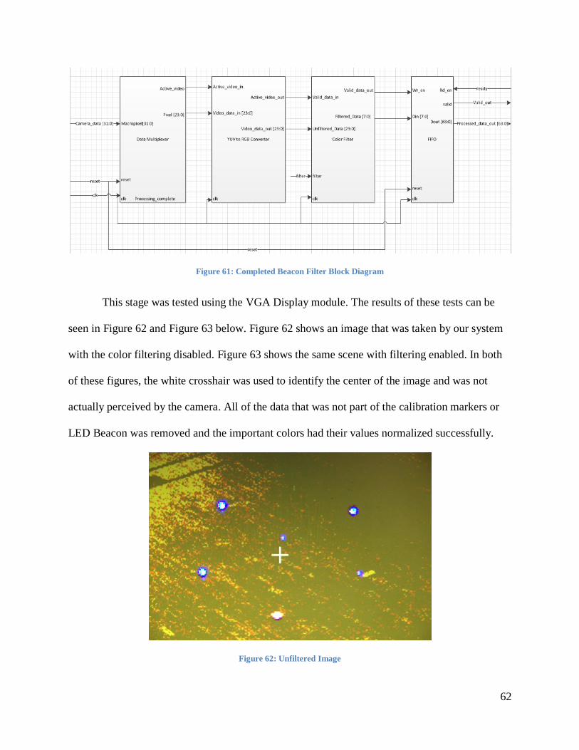
62
Figure 61: Completed Beacon Filter Block Diagram
This stage was tested using the VGA Display module. The results of these tests can be
seen in Figure 62 and Figure 63 below. Figure 62 shows an image that was taken by our system
with the color filtering disabled. Figure 63 shows the same scene with filtering enabled. In both
of these figures, the white crosshair was used to identify the center of the image and was not
actually perceived by the camera. All of the data that was not part of the calibration markers or
LED Beacon was removed and the important colors had their values normalized successfully.
Figure 62: Unfiltered Image
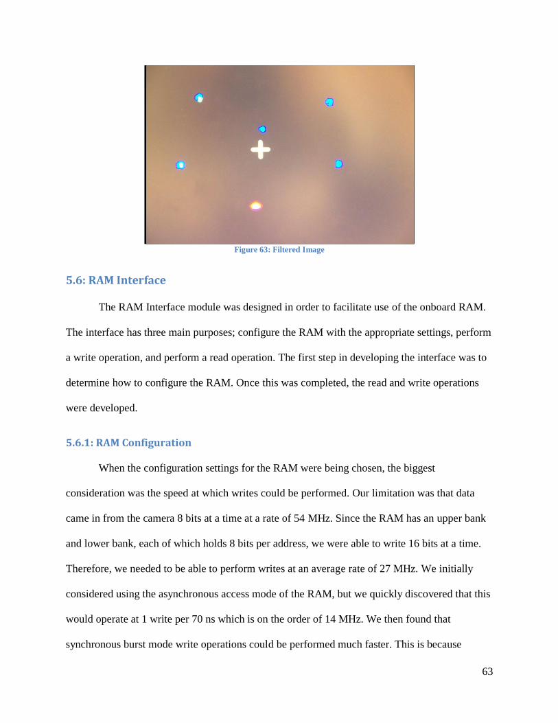
63
Figure 63: Filtered Image
5.6: RAM Interface
The RAM Interface module was designed in order to facilitate use of the onboard RAM.
The interface has three main purposes; configure the RAM with the appropriate settings, perform
a write operation, and perform a read operation. The first step in developing the interface was to
determine how to configure the RAM. Once this was completed, the read and write operations
were developed.
5.6.1: RAM Configuration
When the configuration settings for the RAM were being chosen, the biggest
consideration was the speed at which writes could be performed. Our limitation was that data
came in from the camera 8 bits at a time at a rate of 54 MHz. Since the RAM has an upper bank
and lower bank, each of which holds 8 bits per address, we were able to write 16 bits at a time.
Therefore, we needed to be able to perform writes at an average rate of 27 MHz. We initially
considered using the asynchronous access mode of the RAM, but we quickly discovered that this
would operate at 1 write per 70 ns which is on the order of 14 MHz. We then found that
synchronous burst mode write operations could be performed much faster. This is because
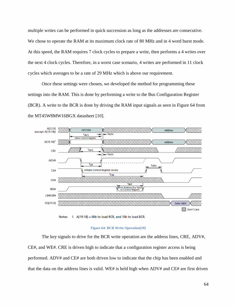
64
multiple writes can be performed in quick succession as long as the addresses are consecutive.
We chose to operate the RAM at its maximum clock rate of 80 MHz and in 4 word burst mode.
At this speed, the RAM requires 7 clock cycles to prepare a write, then performs a 4 writes over
the next 4 clock cycles. Therefore, in a worst case scenario, 4 writes are performed in 11 clock
cycles which averages to be a rate of 29 MHz which is above our requirement.
Once these settings were chosen, we developed the method for programming these
settings into the RAM. This is done by performing a write to the Bus Configuration Register
(BCR). A write to the BCR is done by driving the RAM input signals as seen in Figure 64 from
the MT45W8MW16BGX datasheet [10].
Figure 64: BCR Write Operation[10]
The key signals to drive for the BCR write operation are the address lines, CRE, ADV#,
CE#, and WE#. CRE is driven high to indicate that a configuration register access is being
performed. ADV# and CE# are both driven low to indicate that the chip has been enabled and
that the data on the address lines is valid. WE# is held high when ADV# and CE# are first driven
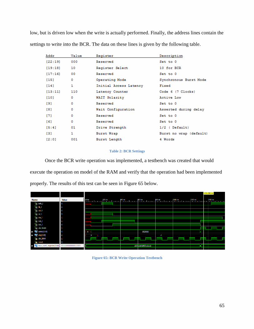
65
low, but is driven low when the write is actually performed. Finally, the address lines contain the
settings to write into the BCR. The data on these lines is given by the following table.
Table 2: BCR Settings
Once the BCR write operation was implemented, a testbench was created that would
execute the operation on model of the RAM and verify that the operation had been implemented
properly. The results of this test can be seen in Figure 65 below.
Figure 65: BCR Write Operation Testbench
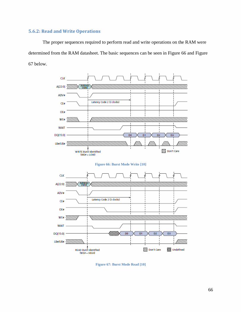
66
5.6.2: Read and Write Operations
The proper sequences required to perform read and write operations on the RAM were
determined from the RAM datasheet. The basic sequences can be seen in Figure 66 and Figure
67 below.
Figure 66: Burst Mode Write [10]
Figure 67: Burst Mode Read [10]
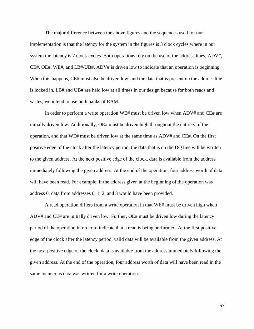
67
The major difference between the above figures and the sequences used for our
implementation is that the latency for the system in the figures is 3 clock cycles where in our
system the latency is 7 clock cycles. Both operations rely on the use of the address lines, ADV#,
CE#, OE#, WE#, and LB#/UB#. ADV# is driven low to indicate that an operation is beginning.
When this happens, CE# must also be driven low, and the data that is present on the address line
is locked in. LB# and UB# are held low at all times in our design because for both reads and
writes, we intend to use both banks of RAM.
In order to perform a write operation WE# must be driven low when ADV# and CE# are
initially driven low. Additionally, OE# must be driven high throughout the entirety of the
operation, and that WE# must be driven low at the same time as ADV# and CE#. On the first
positive edge of the clock after the latency period, the data that is on the DQ line will be written
to the given address. At the next positive edge of the clock, data is available from the address
immediately following the given address. At the end of the operation, four address worth of data
will have been read. For example, if the address given at the beginning of the operation was
address 0, data from addresses 0, 1, 2, and 3 would have been provided.
A read operation differs from a write operation in that WE# must be driven high when
ADV# and CE# are initially driven low. Further, OE# must be driven low during the latency
period of the operation in order to indicate that a read is being performed. At the first positive
edge of the clock after the latency period, valid data will be available from the given address. At
the next positive edge of the clock, data is available from the address immediately following the
given address. At the end of the operation, four address worth of data will have been read in the
same manner as data was written for a write operation.
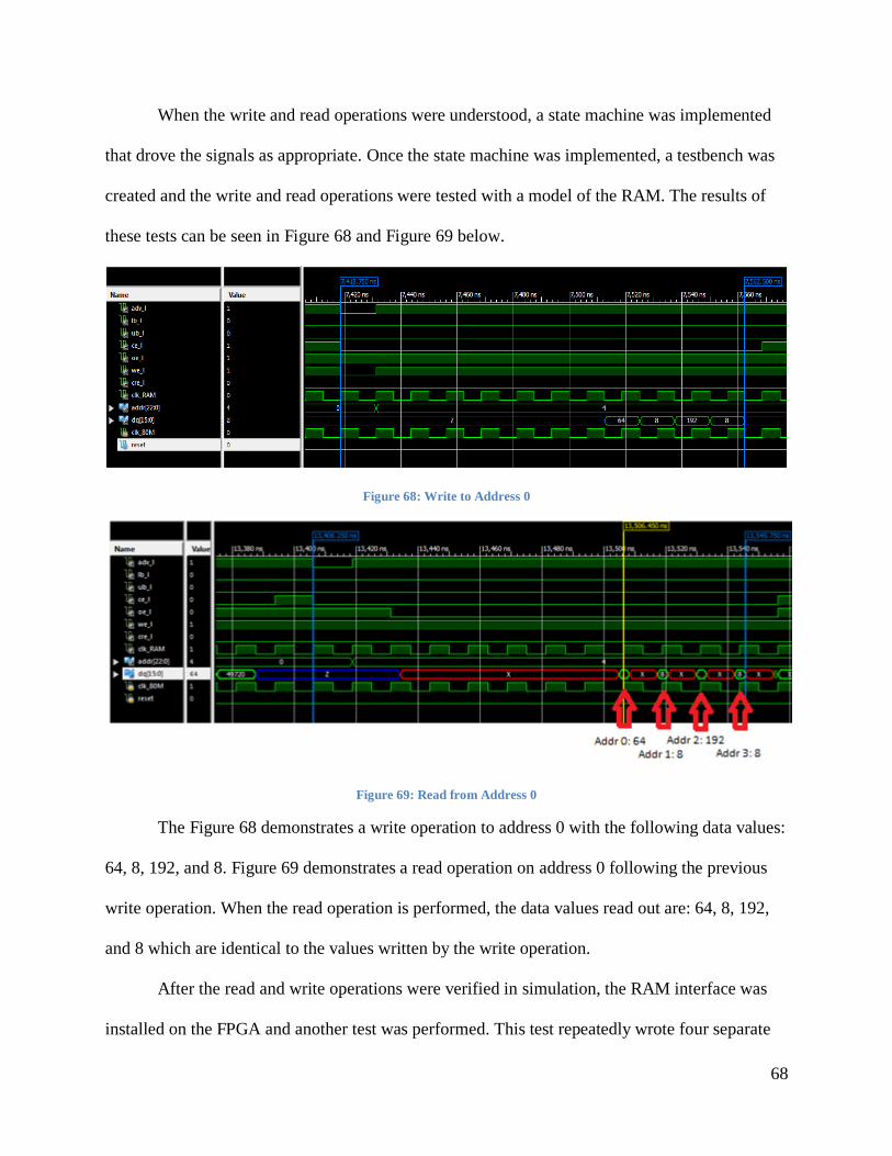
68
When the write and read operations were understood, a state machine was implemented
that drove the signals as appropriate. Once the state machine was implemented, a testbench was
created and the write and read operations were tested with a model of the RAM. The results of
these tests can be seen in Figure 68 and Figure 69 below.
Figure 68: Write to Address 0
Figure 69: Read from Address 0
The Figure 68 demonstrates a write operation to address 0 with the following data values:
64, 8, 192, and 8. Figure 69 demonstrates a read operation on address 0 following the previous
write operation. When the read operation is performed, the data values read out are: 64, 8, 192,
and 8 which are identical to the values written by the write operation.
After the read and write operations were verified in simulation, the RAM interface was
installed on the FPGA and another test was performed. This test repeatedly wrote four separate
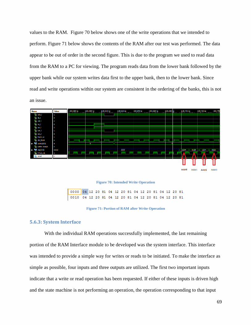
69
values to the RAM. Figure 70 below shows one of the write operations that we intended to
perform. Figure 71 below shows the contents of the RAM after our test was performed. The data
appear to be out of order in the second figure. This is due to the program we used to read data
from the RAM to a PC for viewing. The program reads data from the lower bank followed by the
upper bank while our system writes data first to the upper bank, then to the lower bank. Since
read and write operations within our system are consistent in the ordering of the banks, this is not
an issue.
Figure 70: Intended Write Operation
Figure 71: Portion of RAM after Write Operation
5.6.3: System Interface
With the individual RAM operations successfully implemented, the last remaining
portion of the RAM Interface module to be developed was the system interface. This interface
was intended to provide a simple way for writes or reads to be initiated. To make the interface as
simple as possible, four inputs and three outputs are utilized. The first two important inputs
indicate that a write or read operation has been requested. If either of these inputs is driven high
and the state machine is not performing an operation, the operation corresponding to that input
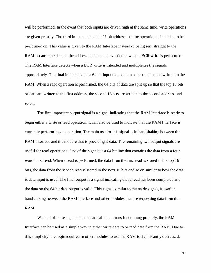
70
will be performed. In the event that both inputs are driven high at the same time, write operations
are given priority. The third input contains the 23 bit address that the operation is intended to be
performed on. This value is given to the RAM Interface instead of being sent straight to the
RAM because the data on the address line must be overridden when a BCR write is performed.
The RAM Interface detects when a BCR write is intended and multiplexes the signals
appropriately. The final input signal is a 64 bit input that contains data that is to be written to the
RAM. When a read operation is performed, the 64 bits of data are split up so that the top 16 bits
of data are written to the first address; the second 16 bits are written to the second address, and
so on.
The first important output signal is a signal indicating that the RAM Interface is ready to
begin either a write or read operation. It can also be used to indicate that the RAM Interface is
currently performing an operation. The main use for this signal is in handshaking between the
RAM Interface and the module that is providing it data. The remaining two output signals are
useful for read operations. One of the signals is a 64 bit line that contains the data from a four
word burst read. When a read is performed, the data from the first read is stored in the top 16
bits, the data from the second read is stored in the next 16 bits and so on similar to how the data
is data input is used. The final output is a signal indicating that a read has been completed and
the data on the 64 bit data output is valid. This signal, similar to the ready signal, is used in
handshaking between the RAM Interface and other modules that are requesting data from the
RAM.
With all of these signals in place and all operations functioning properly, the RAM
Interface can be used as a simple way to either write data to or read data from the RAM. Due to
this simplicity, the logic required in other modules to use the RAM is significantly decreased.
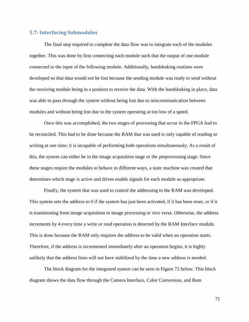
71
5.7: Interfacing Submodules
The final step required to complete the data flow was to integrate each of the modules
together. This was done by first connecting each module such that the output of one module
connected to the input of the following module. Additionally, handshaking routines were
developed so that data would not be lost because the sending module was ready to send without
the receiving module being in a position to receive the data. With the handshaking in place, data
was able to pass through the system without being lost due to miscommunication between
modules and without being lost due to the system operating at too low of a speed.
Once this was accomplished, the two stages of processing that occur in the FPGA had to
be reconciled. This had to be done because the RAM that was used is only capable of reading or
writing at one time; it is incapable of performing both operations simultaneously. As a result of
this, the system can either be in the image acquisition stage or the preprocessing stage. Since
these stages require the modules to behave in different ways, a state machine was created that
determines which stage is active and drives enable signals for each module as appropriate.
Finally, the system that was used to control the addressing to the RAM was developed.
This system sets the address to 0 if the system has just been activated, if it has been reset, or if it
is transitioning from image acquisition to image processing or vice versa. Otherwise, the address
increments by 4 every time a write or read operation is detected by the RAM Interface module.
This is done because the RAM only requires the address to be valid when an operation starts.
Therefore, if the address is incremented immediately after an operation begins, it is highly
unlikely that the address lines will not have stabilized by the time a new address is needed.
The block diagram for the integrated system can be seen in Figure 72 below. This block
diagram shows the data flow through the Camera Interface, Color Conversion, and Ram
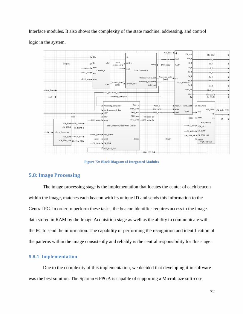
72
Interface modules. It also shows the complexity of the state machine, addressing, and control
logic in the system.
Figure 72: Block Diagram of Integrated Modules
5.8: Image Processing
The image processing stage is the implementation that locates the center of each beacon
within the image, matches each beacon with its unique ID and sends this information to the
Central PC. In order to perform these tasks, the beacon identifier requires access to the image
data stored in RAM by the Image Acquisition stage as well as the ability to communicate with
the PC to send the information. The capability of performing the recognition and identification of
the patterns within the image consistently and reliably is the central responsibility for this stage.
5.8.1: Implementation
Due to the complexity of this implementation, we decided that developing it in software
was the best solution. The Spartan 6 FPGA is capable of supporting a Microblaze soft-core
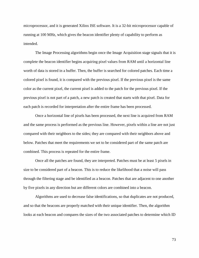
73
microprocessor, and it is generated Xilinx ISE software. It is a 32-bit microprocessor capable of
running at 100 MHz, which gives the beacon identifier plenty of capability to perform as
intended.
The Image Processing algorithms begin once the Image Acquisition stage signals that it is
complete the beacon identifier begins acquiring pixel values from RAM until a horizontal line
worth of data is stored in a buffer. Then, the buffer is searched for colored patches. Each time a
colored pixel is found, it is compared with the previous pixel. If the previous pixel is the same
color as the current pixel, the current pixel is added to the patch for the previous pixel. If the
previous pixel is not part of a patch, a new patch is created that starts with that pixel. Data for
each patch is recorded for interpretation after the entire frame has been processed.
Once a horizontal line of pixels has been processed, the next line is acquired from RAM
and the same process is performed as the previous line. However, pixels within a line are not just
compared with their neighbors to the sides; they are compared with their neighbors above and
below. Patches that meet the requirements we set to be considered part of the same patch are
combined. This process is repeated for the entire frame.
Once all the patches are found, they are interpreted. Patches must be at least 5 pixels in
size to be considered part of a beacon. This is to reduce the likelihood that a noise will pass
through the filtering stage and be identified as a beacon. Patches that are adjacent to one another
by five pixels in any direction but are different colors are combined into a beacon.
Algorithms are used to decrease false identifications, so that duplicates are not produced,
and so that the beacons are properly matched with their unique identifier. Then, the algorithm
looks at each beacon and compares the sizes of the two associated patches to determine which ID
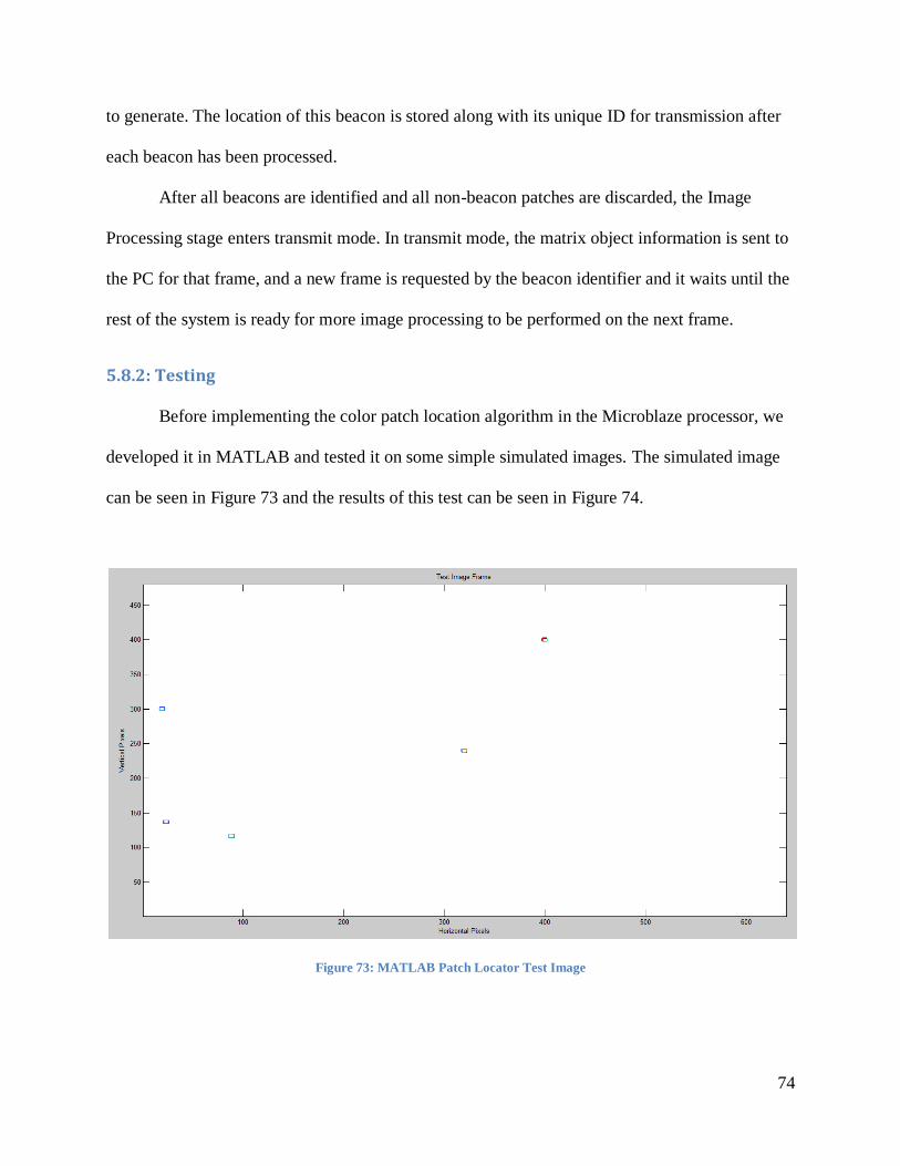
74
to generate. The location of this beacon is stored along with its unique ID for transmission after
each beacon has been processed.
After all beacons are identified and all non-beacon patches are discarded, the Image
Processing stage enters transmit mode. In transmit mode, the matrix object information is sent to
the PC for that frame, and a new frame is requested by the beacon identifier and it waits until the
rest of the system is ready for more image processing to be performed on the next frame.
5.8.2: Testing
Before implementing the color patch location algorithm in the Microblaze processor, we
developed it in MATLAB and tested it on some simple simulated images. The simulated image
can be seen in Figure 73 and the results of this test can be seen in Figure 74.
Figure 73: MATLAB Patch Locator Test Image
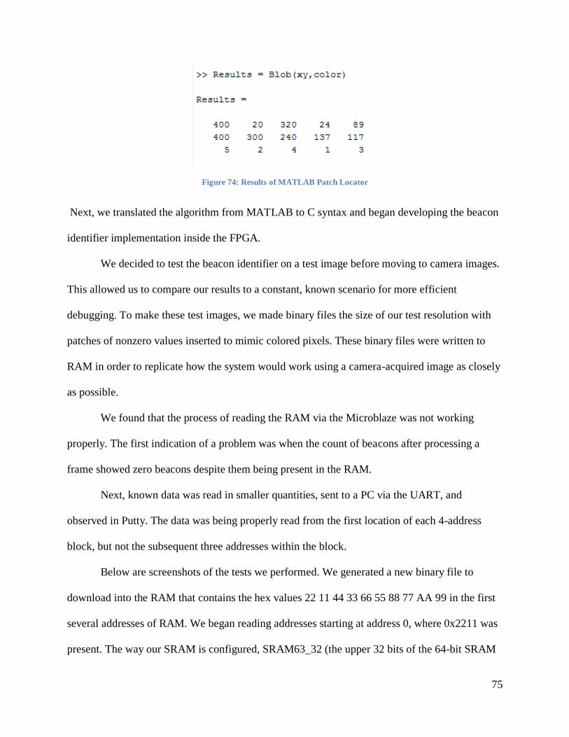
75
Figure 74: Results of MATLAB Patch Locator
Next, we translated the algorithm from MATLAB to C syntax and began developing the beacon
identifier implementation inside the FPGA.
We decided to test the beacon identifier on a test image before moving to camera images.
This allowed us to compare our results to a constant, known scenario for more efficient
debugging. To make these test images, we made binary files the size of our test resolution with
patches of nonzero values inserted to mimic colored pixels. These binary files were written to
RAM in order to replicate how the system would work using a camera-acquired image as closely
as possible.
We found that the process of reading the RAM via the Microblaze was not working
properly. The first indication of a problem was when the count of beacons after processing a
frame showed zero beacons despite them being present in the RAM.
Next, known data was read in smaller quantities, sent to a PC via the UART, and
observed in Putty. The data was being properly read from the first location of each 4-address
block, but not the subsequent three addresses within the block.
Below are screenshots of the tests we performed. We generated a new binary file to
download into the RAM that contains the hex values 22 11 44 33 66 55 88 77 AA 99 in the first
several addresses of RAM. We began reading addresses starting at address 0, where 0x2211 was
present. The way our SRAM is configured, SRAM63_32 (the upper 32 bits of the 64-bit SRAM
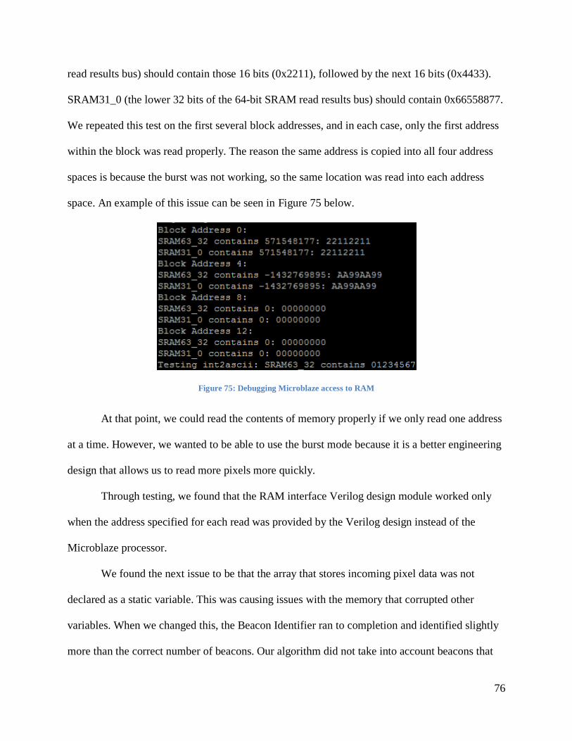
76
read results bus) should contain those 16 bits (0x2211), followed by the next 16 bits (0x4433).
SRAM31_0 (the lower 32 bits of the 64-bit SRAM read results bus) should contain 0x66558877.
We repeated this test on the first several block addresses, and in each case, only the first address
within the block was read properly. The reason the same address is copied into all four address
spaces is because the burst was not working, so the same location was read into each address
space. An example of this issue can be seen in Figure 75 below.
Figure 75: Debugging Microblaze access to RAM
At that point, we could read the contents of memory properly if we only read one address
at a time. However, we wanted to be able to use the burst mode because it is a better engineering
design that allows us to read more pixels more quickly.
Through testing, we found that the RAM interface Verilog design module worked only
when the address specified for each read was provided by the Verilog design instead of the
Microblaze processor.
We found the next issue to be that the array that stores incoming pixel data was not
declared as a static variable. This was causing issues with the memory that corrupted other
variables. When we changed this, the Beacon Identifier ran to completion and identified slightly
more than the correct number of beacons. Our algorithm did not take into account beacons that
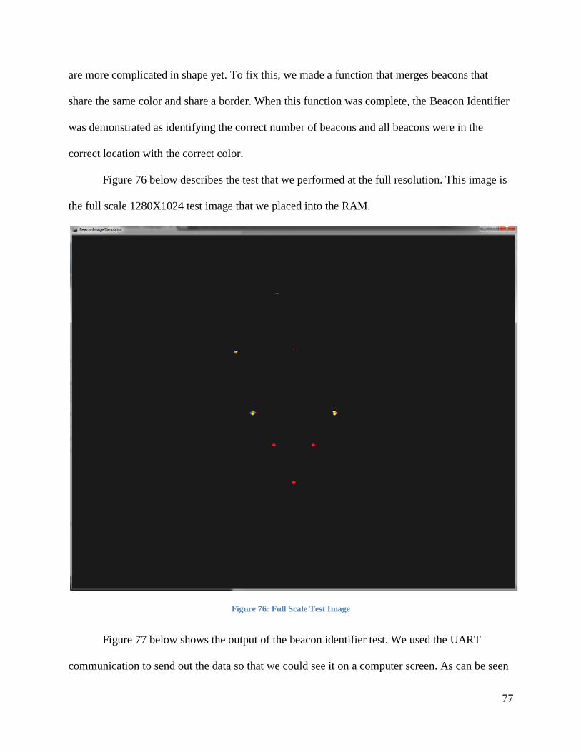
77
are more complicated in shape yet. To fix this, we made a function that merges beacons that
share the same color and share a border. When this function was complete, the Beacon Identifier
was demonstrated as identifying the correct number of beacons and all beacons were in the
correct location with the correct color.
Figure 76 below describes the test that we performed at the full resolution. This image is
the full scale 1280X1024 test image that we placed into the RAM.
Figure 76: Full Scale Test Image
Figure 77 below shows the output of the beacon identifier test. We used the UART
communication to send out the data so that we could see it on a computer screen. As can be seen
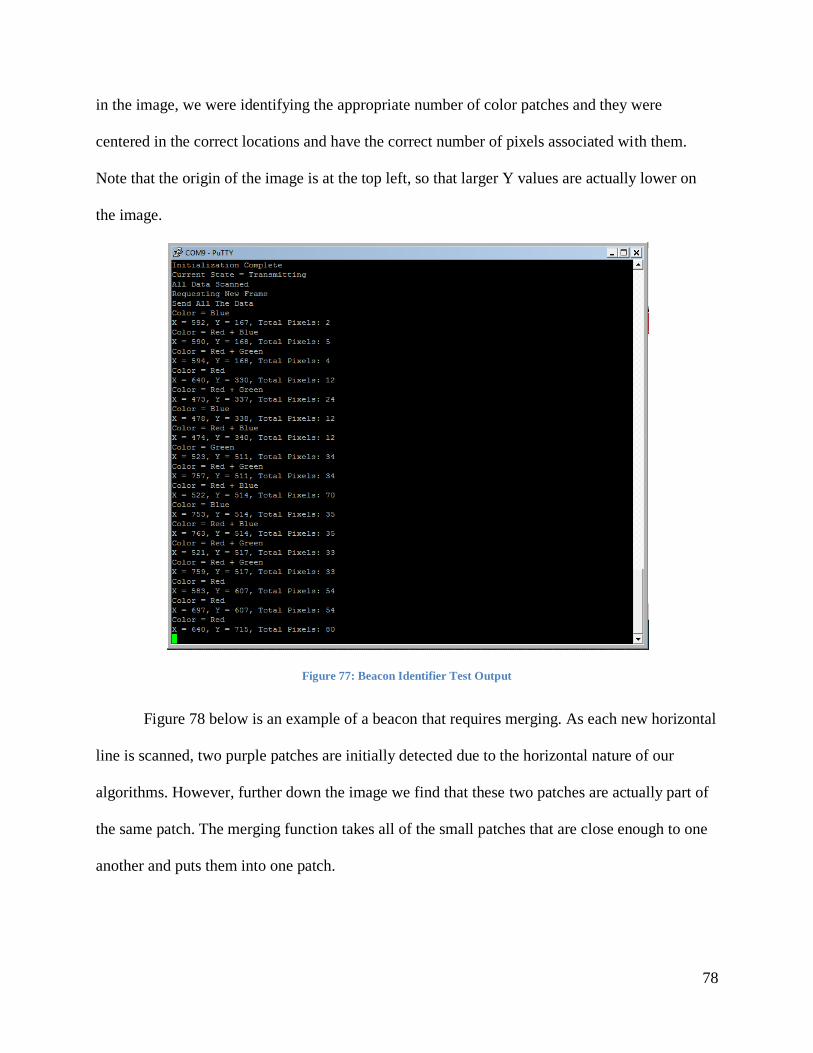
78
in the image, we were identifying the appropriate number of color patches and they were
centered in the correct locations and have the correct number of pixels associated with them.
Note that the origin of the image is at the top left, so that larger Y values are actually lower on
the image.
Figure 77: Beacon Identifier Test Output
Figure 78 below is an example of a beacon that requires merging. As each new horizontal
line is scanned, two purple patches are initially detected due to the horizontal nature of our
algorithms. However, further down the image we find that these two patches are actually part of
the same patch. The merging function takes all of the small patches that are close enough to one
another and puts them into one patch.
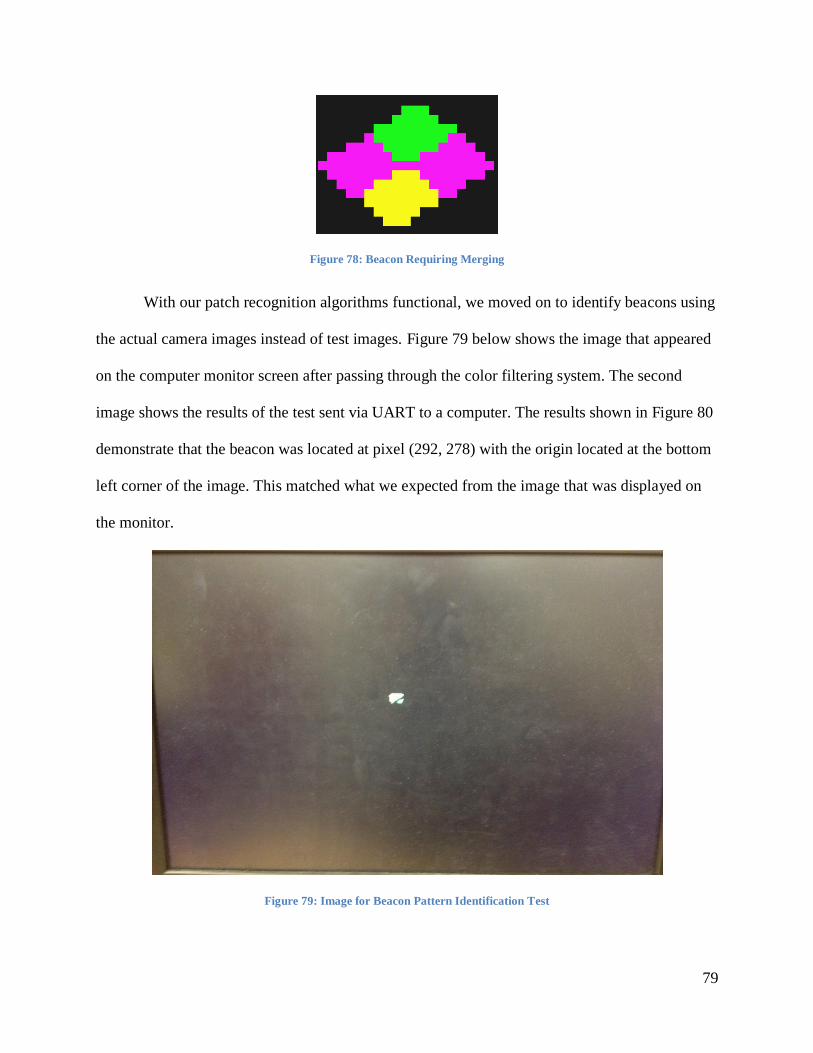
79
Figure 78: Beacon Requiring Merging
With our patch recognition algorithms functional, we moved on to identify beacons using
the actual camera images instead of test images. Figure 79 below shows the image that appeared
on the computer monitor screen after passing through the color filtering system. The second
image shows the results of the test sent via UART to a computer. The results shown in Figure 80
demonstrate that the beacon was located at pixel (292, 278) with the origin located at the bottom
left corner of the image. This matched what we expected from the image that was displayed on
the monitor.
Figure 79: Image for Beacon Pattern Identification Test
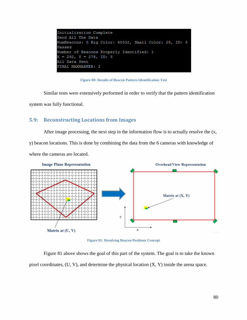
80
Figure 80: Results of Beacon Pattern Identification Test
Similar tests were extensively performed in order to verify that the pattern identification
system was fully functional.
5.9: Reconstructing Locations from Images
After image processing, the next step in the information flow is to actually resolve the (x,
y) beacon locations. This is done by combining the data from the 6 cameras with knowledge of
where the cameras are located.
Figure 81: Resolving Beacon Positions Concept
Figure 81 above shows the goal of this part of the system. The goal is to take the known
pixel coordinates, (U, V), and determine the physical location (X, Y) inside the arena space.
81
5.9.1: Requirements
This stage has several important requirements. It needs to resolve the camera locations
quickly, account for the possibility of the beacons being at a variety of heights, and flexibly
incorporate data from two to six cameras, depending on the beacon's location and the number of
cameras around the field capable of identifying it.
5.9.2: Implementation
Once accurate images could be simulated from a camera pose and object location, we
could move to solve for an object location based on a camera image. Initially, this reconstruction
was developed assuming a height for the beacons. This allowed us to solve for a location with
only one image, however, this seemed to put significant requirements on the FRC teams to
mount the beacons at a specific height, and wouldn't allow our system to compensate for
different terrain heights, which is a feature common in FRC games. These inflexibilities
motivated a solution to use two camera images from different perspectives to first find the height
of the object, and then solve for its (x, y) location as in stereo-vision. Because there are six
cameras present on the field, we developed a solution that to combine the data from all 6 cameras
to generate a least-squares error image reconstruction based on all the images that the object is
located in.
Since a camera image provides horizontal and vertical information (a (u, v) pixel
location), one image can allow us to solve for the (x, y) location of an object, provided we know
the height, z, that the object is located at. This is a case of solving two equations (the mapping to
u pixels, and v pixels), for two unknowns; the x and y positions of the object. However, since
FRC robots vary widely in size, assuming the height of the beacon on the robot is not reasonable.
82
To combat this, we looked to implement a way to combine two camera images to create one 3-
dimensional location.
There were two different methods available to combine image data from two cameras to
solve for an object location. An iterative method would assume a height z, then calculate an (x,
y) location based off of one image, then use the calculated (x, y) and a different image to try to
solve for the z location, and iterate until the (x, y, z) location converged. Since this system needs
to quickly determine the beacon locations, this iterative method did not seem promising, so
principles of stereo-vision were employed to implement a direct method of combining the image
data. This method used the pinhole camera model developed in Chapter 4.3 to express each (u, v)
pixel as a 3D line, L, radiating from the camera's focal point. This is done by expressing the pixel
as a vector by depixelizing it into homogeneous image plane coordinates. Then,
to reverse the homogenization, v is multiplied by a scalar, S, and multiplied by the rotation
matrix which is the inverse of the rotation matrix used to change from <x,y,z> coordinates
to <u,v,w> camera coordinates, and rotates Sv back into <x,y,z> coordinates:
(5.4)
Two different cameras provide two different lines, L1 and L2 pointing to the same object. By
solving for the intersection of L1 and L2, the height of the object z can be determined. Then
using either L1 or L2, the x and y components of the location can be found. This principle is
illustrated in Figure 82 below.
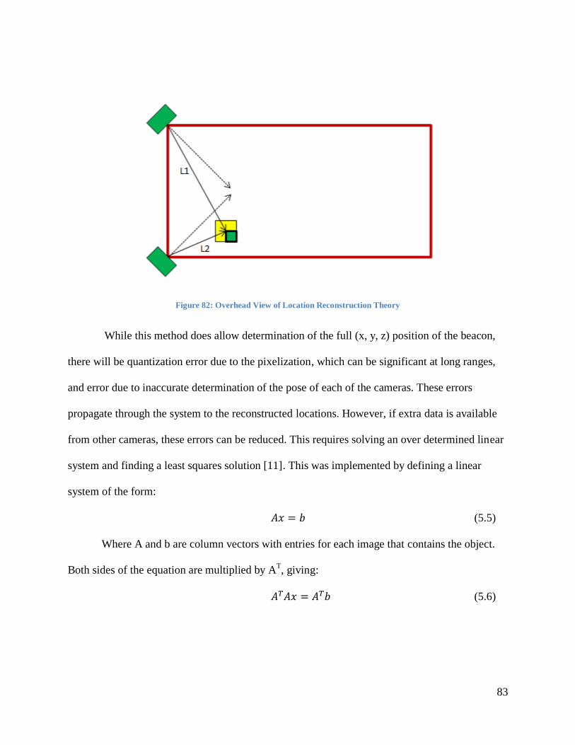
83
Figure 82: Overhead View of Location Reconstruction Theory
While this method does allow determination of the full (x, y, z) position of the beacon,
there will be quantization error due to the pixelization, which can be significant at long ranges,
and error due to inaccurate determination of the pose of each of the cameras. These errors
propagate through the system to the reconstructed locations. However, if extra data is available
from other cameras, these errors can be reduced. This requires solving an over determined linear
system and finding a least squares solution [11]. This was implemented by defining a linear
system of the form:
(5.5)
Where A and b are column vectors with entries for each image that contains the object.
Both sides of the equation are multiplied by AT, giving:
(5.6)
84
Since and are scalar values, solving for
gives the least squares error solution
for x, which is the best possible solution for the object’s location, given the images available.
This calculation is repeated for x, y, and z.
5.9.3: Testing
As this system was implemented, the functionality was continually tested in simulations.
Test images of objects from various perspectives were generated, and those images were used to
reconstruct the beacon locations. The reconstruction was then compared to the actual location the
simulator started with. This procedure was repeated with different image resolutions, camera
locations, lens viewing angles, numbers of cameras, and beacon locations. The results from these
simulations helped guide design decisions regarding the beacon design, camera resolution, and
lens angle.
5.10: Calibration Algorithm
The accuracy of the beacon reconstruction as described above is extremely dependent on
accurately knowing the pose of each camera. Since the system requires installing these cameras
above the floor, it was unreasonable to assume that the cameras would be precision aligned. This
motivated the development of an automated calibration routine, which uses images of objects,
called calibration markers, at known locations inside the field to accurately determine the
camera's pose. The calibration markers are placed temporarily before the competitions until the
calibration is done. The calibration markers are simple blue LEDs. The pose of the camera is
defined as the six parameters that describe the physical orientation of the camera. These are roll,
pitch, yaw, x, y, and z. These parameters are visualized below.
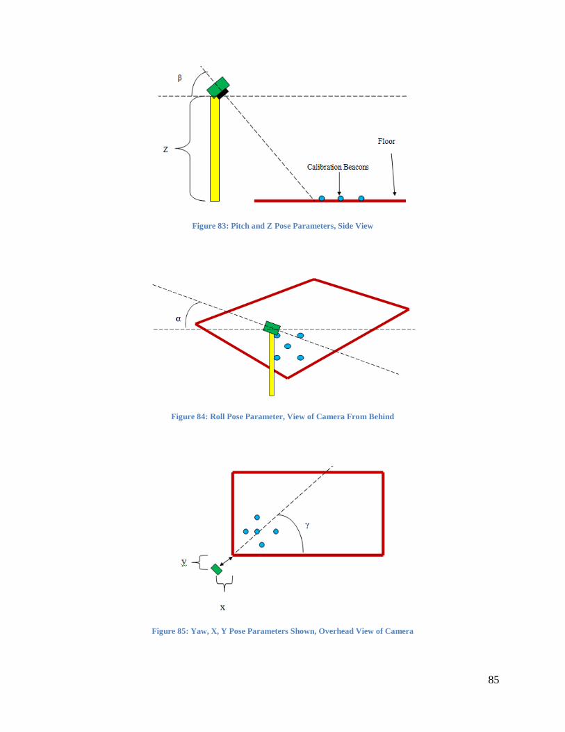
85
Figure 83: Pitch and Z Pose Parameters, Side View
Figure 84: Roll Pose Parameter, View of Camera From Behind
Figure 85: Yaw, X, Y Pose Parameters Shown, Overhead View of Camera
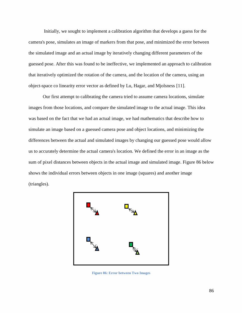
86
Initially, we sought to implement a calibration algorithm that develops a guess for the
camera's pose, simulates an image of markers from that pose, and minimized the error between
the simulated image and an actual image by iteratively changing different parameters of the
guessed pose. After this was found to be ineffective, we implemented an approach to calibration
that iteratively optimized the rotation of the camera, and the location of the camera, using an
object-space co linearity error vector as defined by Lu, Hagar, and Mjolsness [11].
Our first attempt to calibrating the camera tried to assume camera locations, simulate
images from those locations, and compare the simulated image to the actual image. This idea
was based on the fact that we had an actual image, we had mathematics that describe how to
simulate an image based on a guessed camera pose and object locations, and minimizing the
differences between the actual and simulated images by changing our guessed pose would allow
us to accurately determine the actual camera's location. We defined the error in an image as the
sum of pixel distances between objects in the actual image and simulated image. Figure 86 below
shows the individual errors between objects in one image (squares) and another image
(triangles).
Figure 86: Error between Two Images
e e
e e
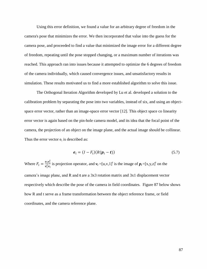
87
Using this error definition, we found a value for an arbitrary degree of freedom in the
camera's pose that minimizes the error. We then incorporated that value into the guess for the
camera pose, and proceeded to find a value that minimized the image error for a different degree
of freedom, repeating until the pose stopped changing, or a maximum number of iterations was
reached. This approach ran into issues because it attempted to optimize the 6 degrees of freedom
of the camera individually, which caused convergence issues, and unsatisfactory results in
simulation. These results motivated us to find a more established algorithm to solve this issue.
The Orthogonal Iteration Algorithm developed by Lu et al. developed a solution to the
calibration problem by separating the pose into two variables, instead of six, and using an object-
space error vector, rather than an image-space error vector [12]. This object space co linearity
error vector is again based on the pin-hole camera model, and its idea that the focal point of the
camera, the projection of an object on the image plane, and the actual image should be collinear.
Thus the error vector ei is described as:
(5.7)
Where
is projection operator, and vi =[u,v,1]t is the image of pi =[x,y,z]
t on the
camera’s image plane, and R and t are a 3x3 rotation matrix and 3x1 displacement vector
respectively which describe the pose of the camera in field coordinates. Figure 87 below shows
how R and t serve as a frame transformation between the object reference frame, or field
coordinates, and the camera reference plane.
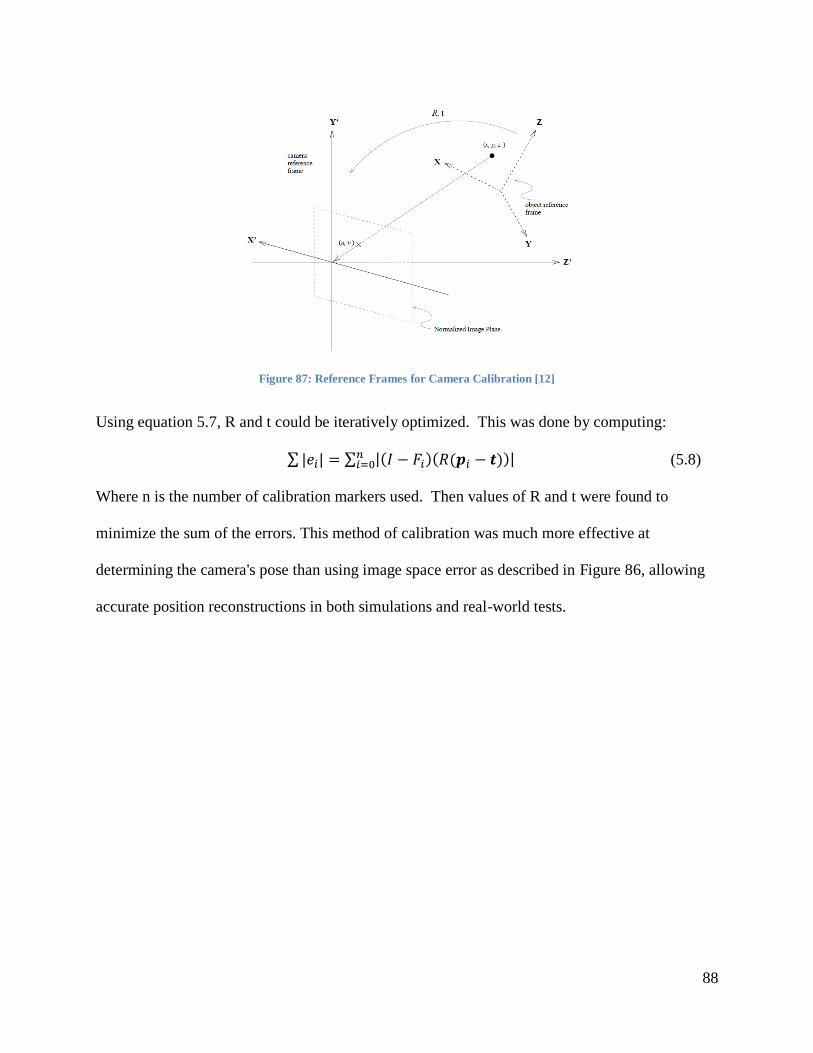
88
Figure 87: Reference Frames for Camera Calibration [12]
Using equation 5.7, R and t could be iteratively optimized. This was done by computing:
(5.8)
Where n is the number of calibration markers used. Then values of R and t were found to
minimize the sum of the errors. This method of calibration was much more effective at
determining the camera's pose than using image space error as described in Figure 86, allowing
accurate position reconstructions in both simulations and real-world tests.

89
Chapter 6: System Testing
With the entirety of the system implemented, we moved on to testing. The system as a
whole was tested in an environment that was meant to emulate a FIRST arena. We used our
single camera to take and process images from locations exactly as they would be positioned in a
real FIRST environment. We placed the LED beacon so that it was visible to three typical
camera locations of our system. This was done to demonstrate the ability to use stereo-vision
concepts incorporating more than two cameras spaced far apart. We also performed tests using
just two cameras. From each camera position, we captured an image of the arena so that it could
be processed offline. We had to process the data offline because we did not have the resources
available to us to replicate our hardware.
Figure 88 shows the testing equipment for viewing the LED beacon and communicating
with the PC. The FPGA board and camera are held inside an acrylic case that we fashioned
specifically to hold these items and support all of our testing operations. The case holding the
camera and FPGA subsystem can be manually tilted and fixed to a certain pose. There is access
to the lens for manual focusing, as well as access to the switches and buttons for mode control.
Two USB wires connect the PC to the FPGA board for development as well as high speed serial
communication.
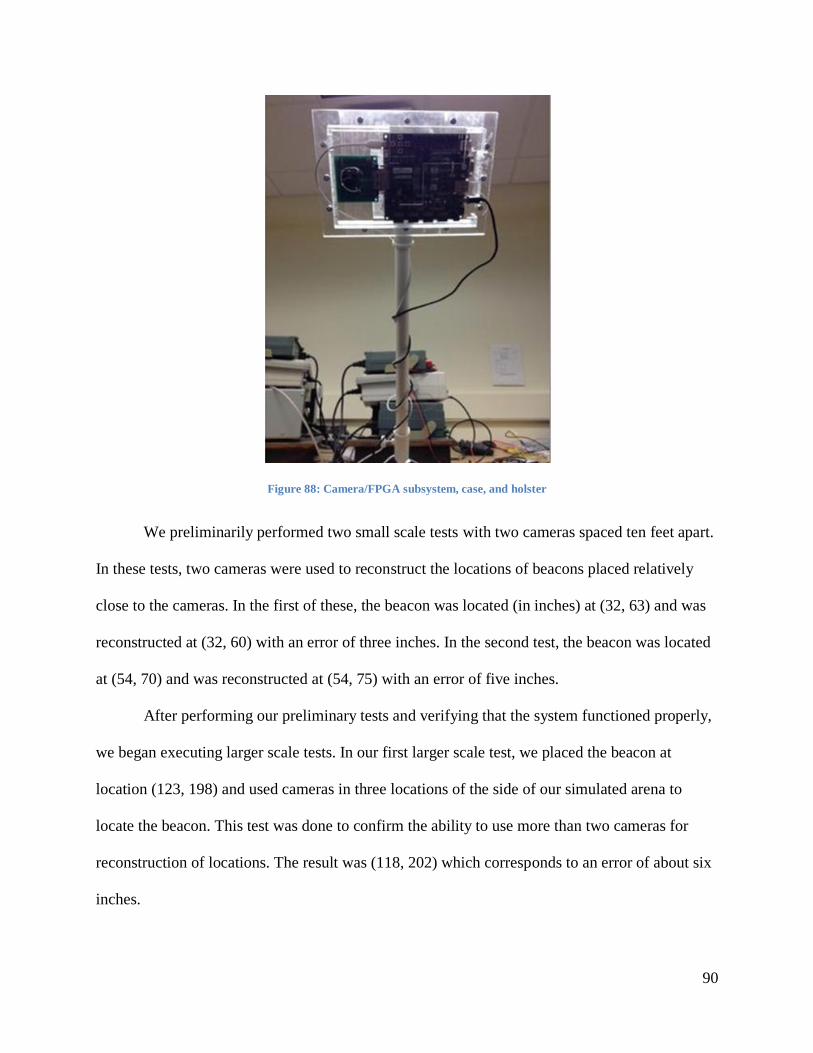
90
Figure 88: Camera/FPGA subsystem, case, and holster
We preliminarily performed two small scale tests with two cameras spaced ten feet apart.
In these tests, two cameras were used to reconstruct the locations of beacons placed relatively
close to the cameras. In the first of these, the beacon was located (in inches) at (32, 63) and was
reconstructed at (32, 60) with an error of three inches. In the second test, the beacon was located
at (54, 70) and was reconstructed at (54, 75) with an error of five inches.
After performing our preliminary tests and verifying that the system functioned properly,
we began executing larger scale tests. In our first larger scale test, we placed the beacon at
location (123, 198) and used cameras in three locations of the side of our simulated arena to
locate the beacon. This test was done to confirm the ability to use more than two cameras for
reconstruction of locations. The result was (118, 202) which corresponds to an error of about six
inches.
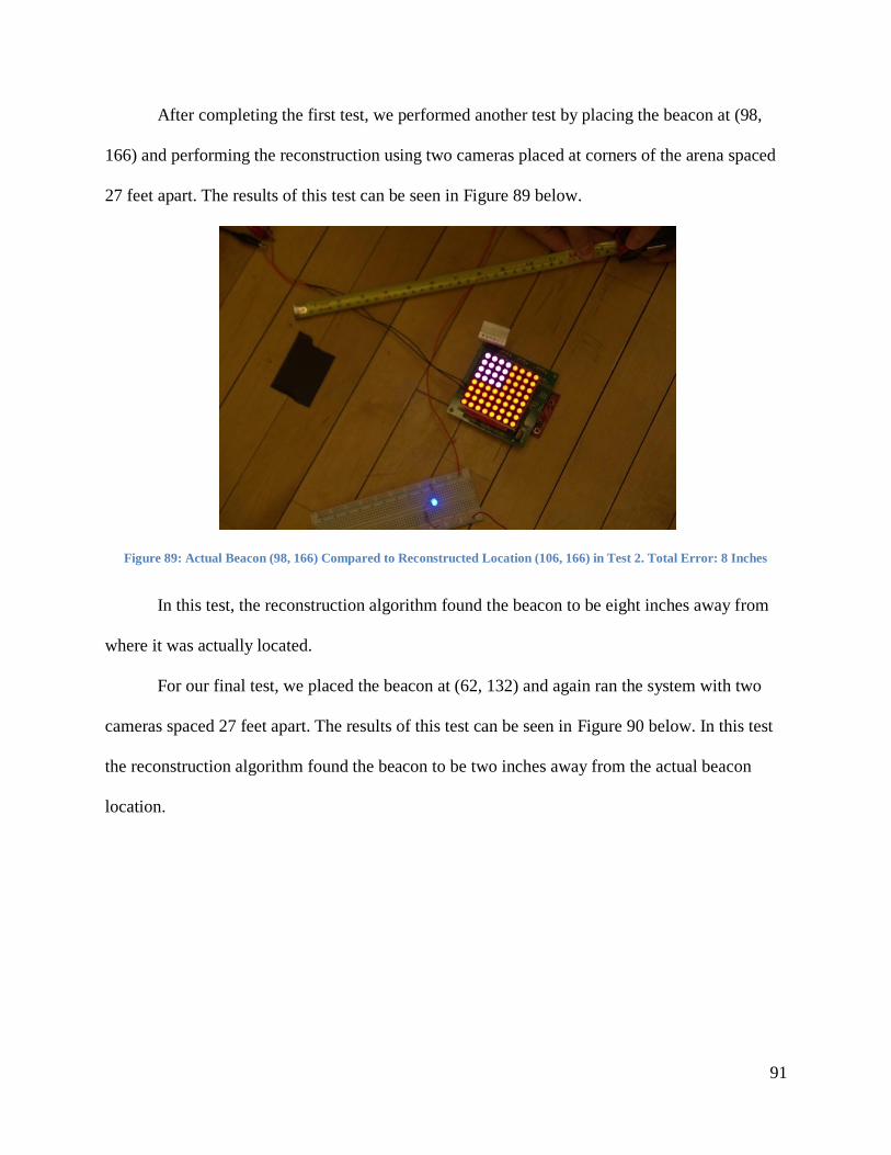
91
After completing the first test, we performed another test by placing the beacon at (98,
166) and performing the reconstruction using two cameras placed at corners of the arena spaced
27 feet apart. The results of this test can be seen in Figure 89 below.
Figure 89: Actual Beacon (98, 166) Compared to Reconstructed Location (106, 166) in Test 2. Total Error: 8 Inches
In this test, the reconstruction algorithm found the beacon to be eight inches away from
where it was actually located.
For our final test, we placed the beacon at (62, 132) and again ran the system with two
cameras spaced 27 feet apart. The results of this test can be seen in Figure 90 below. In this test
the reconstruction algorithm found the beacon to be two inches away from the actual beacon
location.
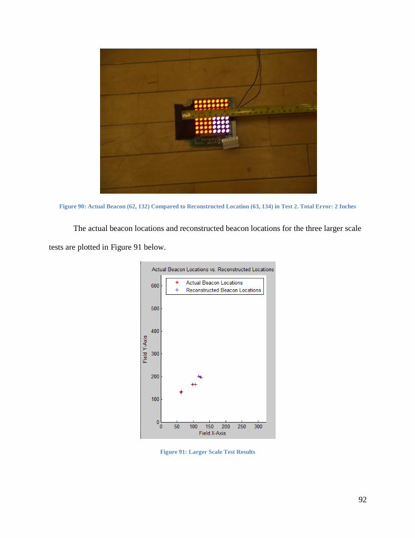
92
Figure 90: Actual Beacon (62, 132) Compared to Reconstructed Location (63, 134) in Test 2. Total Error: 2 Inches
The actual beacon locations and reconstructed beacon locations for the three larger scale
tests are plotted in Figure 91 below.
Figure 91: Larger Scale Test Results
93
After analyzing the results of the tests, we found that the maximum error was 8 inches
and the minimum error was two inches. We believe the range of these results to be due to the fact
that the rig used to hold the camera in place was not entirely stable and the lens of the camera
required focusing between calibration and beacon images. These two factors combined to create
slight errors between the location of the camera as determined by the calibration algorithm and
the actual location of the camera when the reconstruction image was taken. In the FIRST
environment, the cameras would be firmly locked in place, and not require manual focusing
during the competition, and this source of error would be greatly diminished.
94
Chapter 7: Conclusions
The robot localization system we designed and implemented successfully met all of our
system requirements and goals except for a slightly larger error than we were striving for. The
system was carefully designed and developed with the requirements in mind, and the result was a
system that is close to being able to be implemented by FIRST with a minor lens upgrade, and
implementation of an FPGA-based Ethernet controller. The lens would need a larger field of
view to cover the intended area, and the Ethernet controller would enable FIRST to transmit data
across the entire field effectively.
The essential requirement that our system be able to detect and identify all robots
separately was met. This was done by using programmable LED beacons that give twelve unique
patterns for use by the robots. The beacon identification algorithms were successfully able to
identify these patterns in the camera frames and associate them with the appropriate unique
identifier. This was made possible by the very careful design of the embedded FPGA system.
The processes that are run by the FPGA hardware as well as the soft-core Microblaze processor
were extensively planned out before implementation and developed with exhaustive attention to
detail in order to achieve the best possible results for identification.
Testing indicates that the coordinates generated for the beacons are consistently accurate
to eight or fewer inches. While eight inches maximum error is above our ideal accuracy, it is still
reasonably accurate such that it would be of use to the competitors. Additionally, small
variations were present in the system due to human error. This was caused by repeatedly moving
the single camera/FPGA system to multiple locations in order to simulate using multiple
cameras. In a real FIRST environment, the cameras would be held steady and no manual lens
95
adjustment would be required during operation and therefore, the results would be slightly
improved.
The requirement that our system be minimally invasive was met. One way we met this
requirement was to use automated calibration to allow setup to be simple and not force the
volunteers to place the cameras in an extremely precise location. Another way we met this
requirement was to make an LED beacon that is small, light, and low enough in power that it can
be fitted to the robots.
Low maintenance operation was achieved successfully. One way we achieved this was by
adding the capability of powering the beacons using the robots’ on-board power sources to
power the LED beacons. The cameras and their associated embedded systems are powered by a
wall outlet, which is readily accessible at FIRST competitions. The LED beacons are durable
enough for use in the competitions, as long as they are placed on the robots in the right locations
so that they are not hit directly by other robots with excessive force.
The ability of the system to be robust and flexible in a competitive environment was
achieved successfully. This was accomplished primarily inside the image processing embedded
systems. To prevent false identifications or bottlenecking due to excessive data requirements, the
embedded systems filter and normalize the incoming frames specifically to preserve the beacons
and as little background noise as possible. System testing was done inside Harrington
Auditorium as well as inside the MQP lab in different lighting conditions and operation was
consistently smooth.
7.1: Future Work
Testing thus far has been performed by using our single-camera rig to capture images
from multiple locations in order to simulate the effect of having multiple cameras by taking
96
instantaneous snapshots of the test environment. However, the single-camera rigs are all identical
to one another. This means that implementing a full real-time system is possible by simply
replicating our hardware with a minor lens upgrade. Supporting the networking of all six
cameras with the PC over Ethernet would allow FIRST to save money.
The lens available for us during testing did not have the desired field of view or depth of
field. In order to make the full system capable of seeing the entire field, a new lens with the
proper field of view is desired. No modifications to the rest of the hardware would be required to
use a new lens, and only the two lens angle parameters inside the PC source code would need to
be edited.
The range of our tests was limited by the visibility of the beacon. As the beacon was
farther away in the images, the color differences within the LED matrix became obscured. This
meant that the beacon did not appear to have discrete colored sections to the camera, and this
compromised our algorithms. However, a simple and practical solution to this problem would be
to use four LED matrices instead of one. These would be placed in a square pattern, and one
entire LED matrix would be one color, and the other three would be another color. This would
make the smallest quadrant of the matrix four times larger than it is currently, and it would be
seen far more consistently at range. The total beacon size would be six by six inches after the
revision.
97
References
[1] Video. FIRST, 8 Jan. 2011. WMV. <http://www.youtube.com/watch?v=93Tygo0_O5c>.
[2] Digital Image of FIRST arena. Digital image. FIRST Robotics. FIRST Robotics, n.d. Web.
<http://frc-manual.usfirst.org/upload/images/2013/1/Figure2-1.jpg>.
[3] Introduction to Image Processing. Space Telescope. PDF.
<http://www.spacetelescope.org/static/projects/fits_liberator/image_processing.pdf>.
[4] Jisarojito, Jarupat. "Tracking a Robot Using Overhead Cameras for RoboCup SPL League."
[5] Sirota, Alex. Robotracker - A System for Tracking Robots in Real Time. Tech. Technion:
Israel Institute of Technology, 2004.
<http://www.iosart.com/robotracker/RoboTracker.pdf>.
[6] Wang, Meng, and Jean-Yves Herve. "3D Target Tracking Using Multiple Calibrated
Cameras." IEEE Explore. IEEE, n.d. Web.
<http://ieeexplore.ieee.org/stamp/stamp.jsp?tp=&arnumber=4259921>.
[7] Trein, J., A. Th. Schwarzbacher, and B. Hoppe. "FPGA Implementation of a Single Pass
Real-Time Blob Analysis Using Run Length Encoding." School of Electronic and
Communications Engineering. School of Electronic and Communications Engineering,
Feb. 2008. Web. Jan.-Feb. 2013. http://www.electronics.dit.ie/postgrads/jtrein/mpc08-
1Blob.pdf.
[8] "Application Note." Videology Inc. Videology Inc, 1 Apr. 2010. Web. Nov. 2012.
http://www.videologyinc.com/media/products/application%20notes/APN-
24C1.3xDIG.pdf.
[9] Mathworks. "Frame Transformations." Frame Transformations. N.p., 2013. Web. 15 Apr.
2013.

98
[10] Micron. "Async/Page/Burst CellularRAM TM 1.5 MT45W8MW16BGX." N.p., 2004. Web.
[11] Ron, Amos. "Review of Least Squares Solutions to Overdetermined Systems." University
of Wisconsin Madison. University of Wisconsin, 9 Nov. 2010. Web. Mar. 2013.
http://pages.cs.wisc.edu/~amos/412/lecture-notes/lecture17.pdf.
[12] Lu, Chien-Ping, Gregory J. Hager, and Eric Mjolsness. "Fast and Globally Convergent Pose
Estimation From Video Images." The Computable Plant. National Science Foundation
Frontiers in Integrative Biological Research (FIBR) Program, 18 Feb. 1998. Web. Dec.
2012. <http://computableplant.ics.uci.edu/papers/1998/lu98fast.pdf>.
99
Appendix A: Beacon Control Code
The source code below was used to control the patterns displayed on the LED matrix.
This system allowed us to generate unique patterns for each robot which allows multiple robots
to be tracked simultaneously.
#include <msp430g2553.h>
#include <stdio.h>
#include <string.h>
#define row1 BIT0
#define row2 BIT1
#define red1 BIT2
#define red2 BIT3
#define green1 BIT4
#define green2 BIT5
#define blue1 BIT7
#define blue2 BIT6
#define Button BIT3
static int ButtonCount = 0;
static int ulButtons;
static int lastButton = 0;
static int top_bot_actual = 0;
static int top_bot = 0;
static int counter = 0;
void main(void) {
WDTCTL = WDTPW + WDTHOLD;
//reset watch dog timer
TA0CCTL0 = CCIE;
//Timer A0 setup
TA0CTL = TASSEL_2 + MC_1 + ID_3;
TA0CCR0 = 12000;
TA1CCTL0 = CCIE;
//Timer A1 setup
TA1CTL = TASSEL_2 + MC_1 + ID_0;
TA1CCR0 = 124;
_BIS_SR(GIE);
P2SEL &= ~BIT6;
//selecting general I/O
P2SEL &= ~BIT7;
//selecting general I/O
P2OUT = 0;
//setting outputs to 0
100
P2DIR |= row1 + row2 + red1 + red2 + green1 + green2 + blue1 + blue2;
//setting pins to output
P1REN = BIT3;
P1SEL = 0;
P1DIR &= ~BIT3;
P1IN |= BIT3;//read from P1IN port 3 to find out if button's pressed
}
// Timer A0 interrupt service routine
#pragma vector=TIMER0_A0_VECTOR
__interrupt void Timer0_A (void)
{
ulButtons = ((P1IN & Button) != Button);
if((lastButton == 0) && ulButtons)
if(ButtonCount + 1 > 13) // Count up 13 for button press to
change between beacon patterns.
ButtonCount = 0;
else
ButtonCount++;
lastButton = ulButtons;
}
#pragma vector=TIMER1_A0_VECTOR
__interrupt void Timer1_A (void)
{
if(counter > 31)
counter = 0;
else
counter++;
if(top_bot_actual == 0){ //Switches between top set of rows
and bottom set in order to multiplex
top_bot_actual = 1;
}
else {
top_bot_actual = 0;
}
if(counter >= 10) // 12 default
top_bot = 2;
else
top_bot = top_bot_actual;
switch(ButtonCount)
{
case 0:
P2OUT &= row1 + row2;
//Set
Matrix output to be off when powered.
break;
101
case 1:
if(top_bot ==0){
P2OUT &= row2;
P2OUT |= (((~row1 & red1) + row2) | ((~row1 & red2) +
row2)); //Set matrix top row to display red in top left
//and red in top right
}
else if(top_bot == 1){
P2OUT &= row1;
P2OUT |= (((~row2 & red1) + row1) | ((~row2 & red2 +blue2)
+ row1)); //Set matrix bottom row to display red in lower left
//and purple in lower right
}
else
P2OUT &= row1 + row2;
break;
case 2:
if(top_bot ==0){
P2OUT &= row2;
P2OUT |= (((~row1 & red1) + row2) | ((~row1 & red2) +
row2)); //Set matrix top row to display red in top left
//and red in top right
}
else if(top_bot == 1){
P2OUT &= row1;
P2OUT |= (((~row2 & red1) + row1) | ((~row2 & red2 +
green2) + row1)); //Set matrix bottom row to display red in lower left
//and yellow in lower right
}
else
P2OUT &= row1 + row2;
break;
case 3:
if(top_bot ==0){
P2OUT &= row2;
P2OUT |= (((~row1 & red1) + row2) | ((~row1 & red2) +
row2)); //Set matrix top row to display red in top left
//and red in top right
}
else if(top_bot == 1){
P2OUT &= row1;
102
P2OUT |= (((~row2 & red1) + row1) | ((~row2 & green2) +
row1)); //Set matrix bottom row to display red in lower left
//and green in lower right
}
else
P2OUT &= row1 + row2;
break;
case 4:
if(top_bot ==0){
P2OUT &= row2;
P2OUT |= (((~row1 & green1 + red1) + row2) | ((~row1 &
green2 + red2) + row2));//Set matrix top row to display yellow in top left
//and yellow in top right
}
else if(top_bot == 1){
P2OUT &= row1;
P2OUT |= (((~row2 & green1 + red1) + row1) | ((~row2 &
red2) + row1)); //Set matrix bottom row to display yellow in lower left
//and red in lower right
}
else
P2OUT &= row1 + row2;
break;
case 5:
if(top_bot ==0){
P2OUT &= row2;
P2OUT |= (((~row1 & green1 + red1) + row2) | ((~row1 &
green2 + red2) + row2));//Set matrix top row to display yellow in top left
//and yellow in top right
}
else if(top_bot == 1){
P2OUT &= row1;
P2OUT |= (((~row2 & green1 + red1) + row1) | ((~row2 &
green2) + row1)); //Set matrix bottom row to display yellow in lower left
//and green in lower right
}
else
P2OUT &= row1 + row2;
break;
case 6:
if(top_bot ==0){
P2OUT &= row2;
103
P2OUT |= (((~row1 & green1 + red1) + row2) | ((~row1 &
green2 + red2) + row2));//Set matrix top row to display yellow in top left
//and yellow in top right
}
else if(top_bot == 1){
P2OUT &= row1;
P2OUT |= (((~row2 & green1 + red1) + row1) | ((~row2 & red2
+ blue2) + row1));//Set matrix bottom row to display yellow in lower left
//and purple in lower right
}
else
P2OUT &= row1 + row2;
break;
case 7:
if(top_bot ==0){
P2OUT &= row2;
P2OUT |= (((~row1 & green1) + row2) | ((~row1 & green2) +
row2)); //Set matrix top row to display green in top left
//and green in top right
}
else if(top_bot == 1){
P2OUT &= row1;
P2OUT |= (((~row2 & green1) + row1) | ((~row2 & red2) +
row1)); //Set matrix bottom row to display green in lower left
//and red in lower right
}
else
P2OUT &= row1 + row2;
break;
case 8:
if(top_bot == 0){
P2OUT &= row2;
P2OUT |= (((~row1 & green1) + row2) | ((~row1 & green2) +
row2)); //Set matrix top row to display green in top left
//and green in top right
}
else if(top_bot == 1){
P2OUT &= row1;
P2OUT |= (((~row2 & green1) + row1) | ((~row2 & red2 +
green2) + row1)); //Set matrix bottom row to display green in lower left
104
//and yellow in lower right
}
else
P2OUT &= row1 + row2;
break;
case 9:
if(top_bot == 0){
P2OUT &= row2;
P2OUT |= (((~row1 & green1) + row2) | ((~row1 & green2) +
row2)); //Set matrix top row to display green in top left
//and green in top right
}
else if(top_bot == 1){
P2OUT &= row1;
P2OUT |= (((~row2 & green1) + row1) | ((~row2 & red2 +
blue2) + row1)); //Set matrix bottom row to display green in lower left
//and purple in lower right
}
else
P2OUT &= row1 + row2;
break;
case 10:
if(top_bot == 0){
P2OUT &= row2;
P2OUT |= (((~row1 & blue1 + red1) + row2) | ((~row1 & blue2
+ red2) + row2)); //Set matrix top row to display purple in top left
//and purple in top right
}
else if(top_bot == 1){
P2OUT &= row1;
P2OUT |= (((~row2 & blue1 + red1) + row1) | ((~row2 & red2)
+ row1)); //Set matrix bottom row to display purple in lower left
//and red in lower right
}
else
P2OUT &= row1 + row2;
break;
case 11:
if(top_bot == 0){
P2OUT &= row2;
105
P2OUT |= (((~row1 & blue1 + red1) + row2) | ((~row1 & blue2
+ red2) + row2)); //Set matrix top row to display purple in top left
//and purple in top right
}
else if(top_bot == 1){
P2OUT &= row1;
P2OUT |= (((~row2 & blue1 + red1) + row1) | ((~row2 &
green2 + red2) + row1)); //Set matrix bottom row to display purple
in lower left
//and yellow in lower right
}
else
P2OUT &= row1 + row2;
break;
case 12:
if(top_bot == 0){
P2OUT &= row2;
P2OUT |= (((~row1 & blue1 + red1) + row2) | ((~row1 & blue2
+ red2) + row2)); //Set matrix top row to display purple in top left
//and purple in top right
}
else if(top_bot == 1){
P2OUT &= row1;
P2OUT |= (((~row2 & blue1 + red1) + row1) | ((~row2 &
green2) + row1)); //Set matrix bottom row to display purple in lower left
//and green in lower right
}
else
P2OUT &= row1 + row2;
break;
}
}
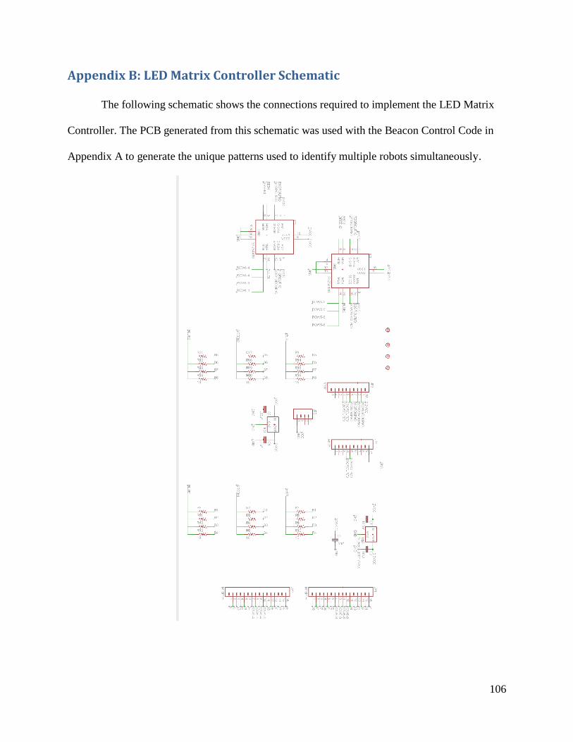
106
Appendix B: LED Matrix Controller Schematic
The following schematic shows the connections required to implement the LED Matrix
Controller. The PCB generated from this schematic was used with the Beacon Control Code in
Appendix A to generate the unique patterns used to identify multiple robots simultaneously.
107
Appendix C: Verilog Modules
The Verilog code below is the top level module that was implemented for the Image
Acquisition and Image Processing stages. These stages were used to interface with the camera,
store frames, and process the images for each camera. This is only a small subsection of the
Verilog design in order to keep the size of this report manageable. The full source code for this
design is available if requested. The names of the other Verilog Modules used in this system are:
Camera_In, Processing, RAM_Interface, and VGA_Display.
`timescale 1ns / 1ps
// This module is the top level module for the Image Acquisition and
// Image Processing stages of the system. In this module, data is taken
// from the camera in YUV format, converted to RGB format and stored in
// RAM. After a frame has been stored in RAM, the Microblaze begins
// processing the image to determine the center of each beacon and which
// pattern it is displaying. Once this is complete, the data is sent via
// UART communications to a Central PC for processing.
module top_level(
input FPGA_clk,
input reset,
input next_frame,
input dclk,
input HREF,
input VREF,
input filter,
input auto_mode,
input UART_Rx,
input [2:0] switch,
input [7:0] din,
output adv_l,
output lb_l,
output ub_l,
output ce_l,
output oe_l,
output we_l,
output cre_l,
output flash_ce,
output clk_RAM,
output HS,
output VS,
output UART_Tx,
output [7:0] VGA_Color,
output [7:0] led,
output [22:0] addr,
inout [15:0] dq
);
108
// Horizontal Pixel Resolution
parameter HPIXELS = 640;
// Vertical Pixel Resolution
parameter VPIXELS = 480;
// Total number of pixels in frame based on HPIXELS and VPIXELS
parameter NUM_PIXELS = HPIXELS*VPIXELS;
// Values assigned to state labels
parameter [2:0] WAIT_STATE = 0, CAMERA_DATA = 1, FINAL_DATA = 2,
MICROBLAZE = 3, VGA_DISPLAY = 4;
wire ready;
wire valid_camera_data;
wire valid_processed_data;
wire clk_80M;
wire processing_complete;
wire display;
wire data_valid;
wire VGA_FIFO_Full;
wire FIFO_reset;
wire powering_up;
wire clk_25M_180;
wire clk_54M;
wire clk_25M;
wire ready_2;
wire auto_next_frame;
wire microblaze_active;
wire blob_next_frame;
wire blob_read;
wire [31:0] camera_data;
wire [63:0] processed_data;
wire [63:0] RAM_dout;
wire [6:0] led_outputs;
wire [31:0] GPI1, GPI2, GPI3;
wire [31:0] GPO1;
reg last_ready;
reg last_VREF;
reg last_read;
reg [2:0] last_state;
reg [2:0] current_state, next_state;
reg [11:0] HLimit;
reg [22:0] addr_in;
reg [24:0] timer;
// clk_converter takes in 100 MHz clock input and creates other clock
signals.
clk_converter inst_clk_converter (
.CLK_IN1(FPGA_clk), // In - 100 MHz clock
.clk_100M(clk_100M), // Out - 100 MHz clock
.clk_80M(clk_80M), // Out - 80 MHz clock
.clk_25M(clk_25M), // Out - 25 MHz clock
.clk_25M_180(clk_25M_180) // Out - 25 MHz clock 180 degree phase
shift
);
// Camera_In receives data from the camera and packages macropixels together
109
Camera_In inst_Camera_In(
.clk(dclk), // In - 54 MHz clock
.reset(FIFO_reset), // In - Reset
.read(Camera_In_read), // In - FIFO read signal
.write(Camera_In_write), // In - FIFO write signal
.din(din), // Out - Image data [7:0]
.valid(valid_camera_data), // Out - FIFO valid
.dout(camera_data) // Out - Macropixel of data [31:0]
);
// Processing module converts from YUV to RGB and applies filters
Processing inst_Processing(
.clk(clk_80M), // In - 80 MHz clock
.valid_in(valid_camera_data), // In - Valid data
.filter(filter), // In - Activate Filtering
.reset(FIFO_reset), // In - Reset
.ready(ready_2), // In - FIFO read control. RAM ready for data
.camera_data(camera_data), // In - Image Data [23:0]
.valid_out(valid_processed_data), // Out - Valid data on output
.processed_data_out(processed_data), // Out - Processed data [63:0]
.processing_complete(processing_complete) // Out - Processing has
finished
);
// Performs RAM reads and writes
RAM_Interface inst_RAM_interface(
.din(processed_data), // In - Din [63:0]
.read(RAM_read), // In - Read command
.write(RAM_write), // In - Write command
.clk(clk_80M), // In - 80 MHz clock
.reset(reset), // In - Reset
.addr_in(addr_in), // In - Address [22:0]
.clk_out(clk_RAM), // Out - 80 MHz clock
.adv_l(adv_l), // Out - Adv
.lb_l(lb_l), // Out - LB
.ub_l(ub_l), // Out - UB
.ce_l(ce_l), // Out - CE
.oe_l(oe_l), // Out - OE
.we_l(we_l), // Out - WE
.cre_l(cre_l), // Out - CRE
.flash_ce(flash_ce), // Out - Flash CE
.ready(ready), // Out - Ready for operation
.dout_valid(data_valid), // Out - Output data valid
.powering_up(powering_up), // Out - RAM is in powering up state
.addr_out(addr), // Out - Address to RAM
.dout(RAM_dout), // Out - Dout [63:0]
.dq(dq) // InOut - RAM data line [15:0]
);
// Microblaze soft-core processor
MCS mcs_0 (
.Clk(clk_100M), // IN - 100 MHz clock
.Reset(reset), // In - Reset
.UART_Rx(UART_Rx), // In - UART_Rx
.UART_Tx(UART_Tx), // Out - UART_Tx
.GPO1(GPO1), // Out - [31 : 0] GPO1
110
.GPI1(GPI1), // In - [31 : 0] GPI1
.GPI1_Interrupt(), // Out - GPI1_Interrupt
.GPI2(GPI2), // In - [31 : 0] GPI2
.GPI2_Interrupt(), // Out - GPI2_Interrupt
.GPI3(GPI3), // In - [31 : 0] GPI3
.GPI3_Interrupt() // Out - GPI3_Interrupt
);
// VGA control module
VGA_Display inst_VGA_Display(
.reset(reset), // In - Reset
.VGA_clk(clk_25M), // In - 25 MHz clock
.clk_25M_180(clk_25M_180),// In - 180 degree out of phase 25 MHz clock
.clk_80M(clk_80M), // In - 80 MHz clock
.display(display), // In - Display active
.data_valid(data_valid), // In - RAM data valid
.data(RAM_dout), // In - RAM data [63:0]
.VGA_FIFO_Full(VGA_FIFO_Full), // Out - FIFO full
.HS(HS), // Out - Horizontal Sync
.VS(VS), // Out - Vertical Sync
.VGA_Color(VGA_Color) // Out - Pixel color [7:0]
);
// Limit number of pixels per line to HPIXELS
always @(posedge dclk)
begin
if(~HREF)
HLimit <= 0;
else
HLimit <= HLimit + 1'b1;
end
// Pulse detection for microblaze RAM read
always @(posedge clk_80M)
last_read <= blob_read;
// Increment addr
always @(posedge clk_80M)
begin
last_ready <= ready;
if((last_state == FINAL_DATA && current_state == MICROBLAZE) ||
(last_state == MICROBLAZE && current_state == VGA_DISPLAY) || reset ||
(current_state == VGA_DISPLAY && ~VS))
addr_in <= 0;
else if(current_state != WAIT_STATE)
begin
if((~ready && last_ready))
begin
if(addr_in + 3'h4 < NUM_PIXELS/2-1)
addr_in <= addr_in + 3'h4;
else
addr_in <= 0;
end
end
else
addr_in <= 0;
end
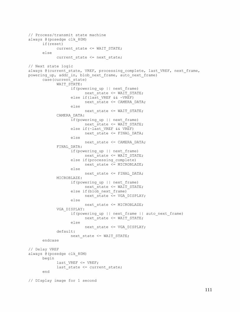
111
// Process/transmit state machine
always @(posedge clk_80M)
if(reset)
current_state <= WAIT_STATE;
else
current_state <= next_state;
// Next state logic
always @(current_state, VREF, processing_complete, last_VREF, next_frame,
powering_up, addr_in, blob_next_frame, auto_next_frame)
case(current_state)
WAIT_STATE:
if(powering_up || next_frame)
next_state <= WAIT_STATE;
else if(last_VREF && ~VREF)
next_state <= CAMERA_DATA;
else
next_state <= WAIT_STATE;
CAMERA_DATA:
if(powering_up || next_frame)
next_state <= WAIT_STATE;
else if(~last_VREF && VREF)
next_state <= FINAL_DATA;
else
next_state <= CAMERA_DATA;
FINAL_DATA:
if(powering_up || next_frame)
next_state <= WAIT_STATE;
else if(processing_complete)
next_state <= MICROBLAZE;
else
next_state <= FINAL_DATA;
MICROBLAZE:
if(powering_up || next_frame)
next_state <= WAIT_STATE;
else if(blob_next_frame)
next_state <= VGA_DISPLAY;
else
next_state <= MICROBLAZE;
VGA_DISPLAY:
if(powering_up || next_frame || auto_next_frame)
next_state <= WAIT_STATE;
else
next_state <= VGA_DISPLAY;
default:
next_state <= WAIT_STATE;
endcase
// Delay VREF
always @(posedge clk_80M)
begin
last_VREF <= VREF;
last_state <= current_state;
end
// DIsplay image for 1 second
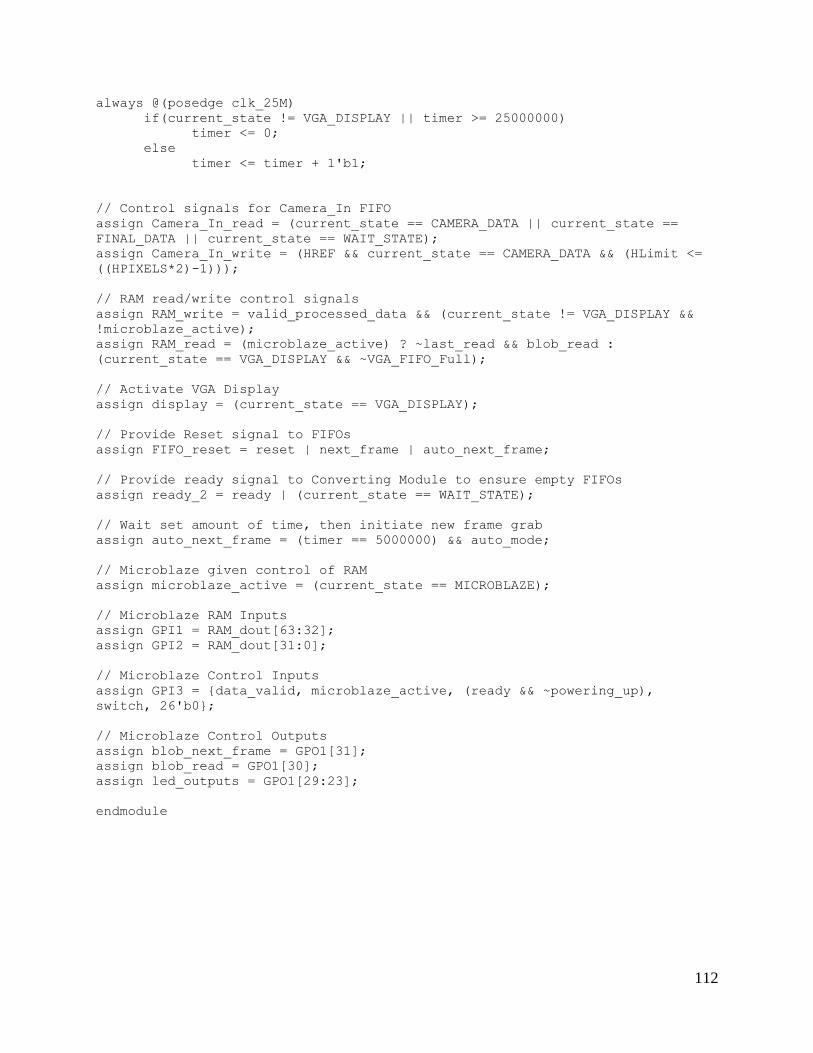
112
always @(posedge clk_25M)
if(current_state != VGA_DISPLAY || timer >= 25000000)
timer <= 0;
else
timer <= timer + 1'b1;
// Control signals for Camera_In FIFO
assign Camera_In_read = (current_state == CAMERA_DATA || current_state ==
FINAL_DATA || current_state == WAIT_STATE);
assign Camera_In_write = (HREF && current_state == CAMERA_DATA && (HLimit <=
((HPIXELS*2)-1)));
// RAM read/write control signals
assign RAM_write = valid_processed_data && (current_state != VGA_DISPLAY &&
!microblaze_active);
assign RAM_read = (microblaze_active) ? ~last_read && blob_read :
(current_state == VGA_DISPLAY && ~VGA_FIFO_Full);
// Activate VGA Display
assign display = (current_state == VGA_DISPLAY);
// Provide Reset signal to FIFOs
assign FIFO_reset = reset | next_frame | auto_next_frame;
// Provide ready signal to Converting Module to ensure empty FIFOs
assign ready_2 = ready | (current_state == WAIT_STATE);
// Wait set amount of time, then initiate new frame grab
assign auto_next_frame = (timer == 5000000) && auto_mode;
// Microblaze given control of RAM
assign microblaze_active = (current_state == MICROBLAZE);
// Microblaze RAM Inputs
assign GPI1 = RAM_dout[63:32];
assign GPI2 = RAM_dout[31:0];
// Microblaze Control Inputs
assign GPI3 = {data_valid, microblaze_active, (ready && ~powering_up),
switch, 26'b0};
// Microblaze Control Outputs
assign blob_next_frame = GPO1[31];
assign blob_read = GPO1[30];
assign led_outputs = GPO1[29:23];
endmodule
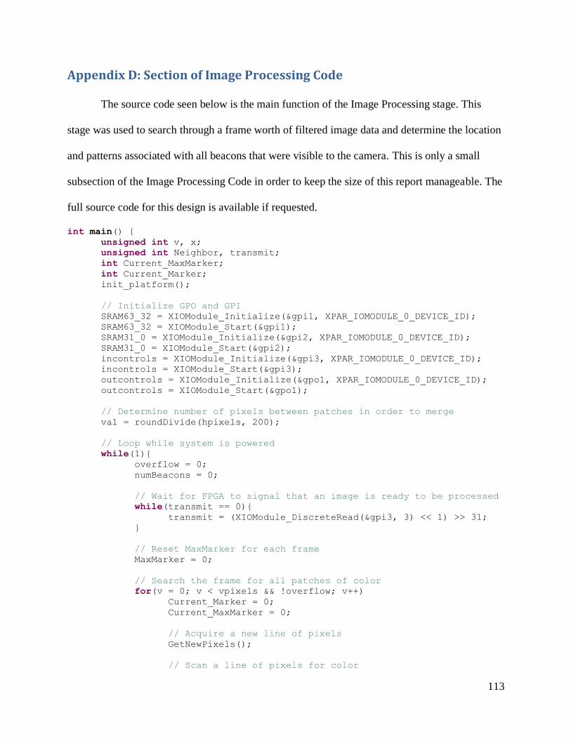
113
Appendix D: Section of Image Processing Code
The source code seen below is the main function of the Image Processing stage. This
stage was used to search through a frame worth of filtered image data and determine the location
and patterns associated with all beacons that were visible to the camera. This is only a small
subsection of the Image Processing Code in order to keep the size of this report manageable. The
full source code for this design is available if requested.
int main() {
unsigned int v, x;
unsigned int Neighbor, transmit;
int Current_MaxMarker;
int Current_Marker;
init_platform();
// Initialize GPO and GPI
SRAM63_32 = XIOModule_Initialize(&gpi1, XPAR_IOMODULE_0_DEVICE_ID);
SRAM63_32 = XIOModule_Start(&gpi1);
SRAM31_0 = XIOModule_Initialize(&gpi2, XPAR_IOMODULE_0_DEVICE_ID);
SRAM31_0 = XIOModule_Start(&gpi2);
incontrols = XIOModule_Initialize(&gpi3, XPAR_IOMODULE_0_DEVICE_ID);
incontrols = XIOModule_Start(&gpi3);
outcontrols = XIOModule_Initialize(&gpo1, XPAR_IOMODULE_0_DEVICE_ID);
outcontrols = XIOModule_Start(&gpo1);
// Determine number of pixels between patches in order to merge
val = roundDivide(hpixels, 200);
// Loop while system is powered
while(1){
overflow = 0;
numBeacons = 0;
// Wait for FPGA to signal that an image is ready to be processed
while(transmit == 0){
transmit = (XIOModule_DiscreteRead(&gpi3, 3) << 1) >> 31;
}
// Reset MaxMarker for each frame
MaxMarker = 0;
// Search the frame for all patches of color
for(v = 0; v < vpixels && !overflow; v++)
Current_Marker = 0;
Current_MaxMarker = 0;
// Acquire a new line of pixels
GetNewPixels();
// Scan a line of pixels for color
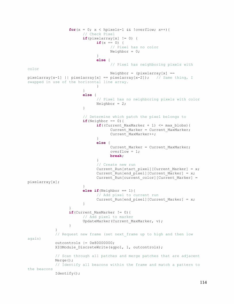
114
for(x = 0; x < hpixels-1 && !overflow; x++){
// Check Pixel
if(pixelarray[x] != 0) {
if(x == 0) {
// Pixel has no color
Neighbor = 0;
}
else {
// Pixel has neighboring pixels with
color
Neighbor = (pixelarray[x] ==
pixelarray[x-1] || pixelarray[x] == pixelarray[x-2]); // Same thing, I
swapped in use of the horizontal line array.
}
}
else {
// Pixel has no neighboring pixels with color
Neighbor = 2;
}
// Determine which patch the pixel belongs to
if(Neighbor == 0){
if((Current_MaxMarker + 1) <= max_blobs){
Current_Marker = Current_MaxMarker;
Current_MaxMarker++;
}
else {
Current_Marker = Current_MaxMarker;
overflow = 1;
break;
}
// Create new run
Current_Run[start_pixel][Current_Marker] = x;
Current_Run[end_pixel][Current_Marker] = x;
Current_Run[current_color][Current_Marker] =
pixelarray[x];
}
else if(Neighbor == 1){
// Add pixel to current run
Current_Run[end_pixel][Current_Marker] = x;
}
}
if(Current_MaxMarker != 0){
// Add pixel to marker
UpdateMarker(Current_MaxMarker, v);
}
}
// Request new frame (set next_frame up to high and then low
again)
outcontrols |= 0x80000000;
XIOModule_DiscreteWrite(&gpo1, 1, outcontrols);
// Scan through all patches and merge patches that are adjacent
Merge();
// Identify all beacons within the frame and match a pattern to
the beacons
Identify();
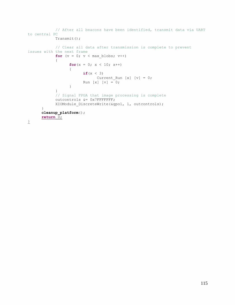
115
// After all beacons have been identified, transmit data via UART
to central PC
Transmit();
// Clear all data after transmission is complete to prevent
issues with the next frame
for (v = 0; v < max_blobs; v++)
{
for(x = 0; x < 10; x++)
{
if(x < 3)
Current_Run [x] [v] = 0;
Run [x] [v] = 0;
}
}
// Signal FPGA that image processing is complete
outcontrols &= 0x7FFFFFFF;
XIOModule_DiscreteWrite(&gpo1, 1, outcontrols);
}
cleanup_platform();
return 0;
}
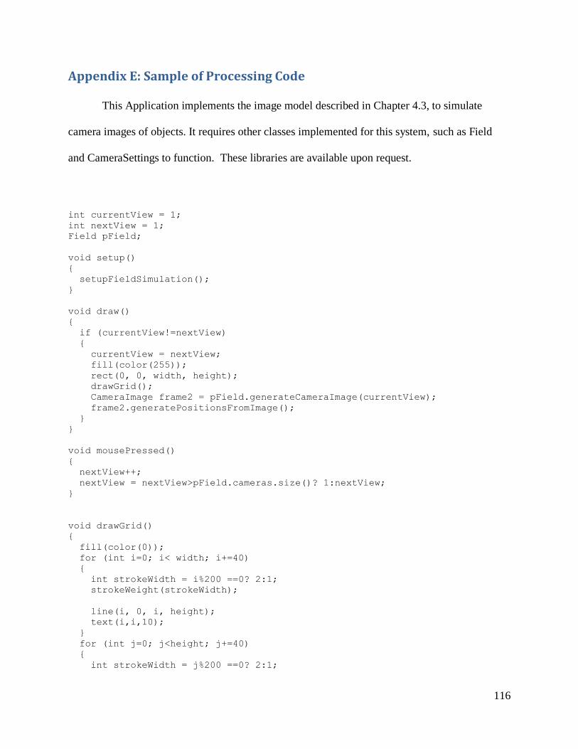
116
Appendix E: Sample of Processing Code
This Application implements the image model described in Chapter 4.3, to simulate
camera images of objects. It requires other classes implemented for this system, such as Field
and CameraSettings to function. These libraries are available upon request.
int currentView = 1;
int nextView = 1;
Field pField;
void setup()
{
setupFieldSimulation();
}
void draw()
{
if (currentView!=nextView)
{
currentView = nextView;
fill(color(255));
rect(0, 0, width, height);
drawGrid();
CameraImage frame2 = pField.generateCameraImage(currentView);
frame2.generatePositionsFromImage();
}
}
void mousePressed()
{
nextView++;
nextView = nextView>pField.cameras.size()? 1:nextView;
}
void drawGrid()
{
fill(color(0));
for (int i=0; i< width; i+=40)
{
int strokeWidth = i%200 ==0? 2:1;
strokeWeight(strokeWidth);
line(i, 0, i, height);
text(i,i,10);
}
for (int j=0; j<height; j+=40)
{
int strokeWidth = j%200 ==0? 2:1;
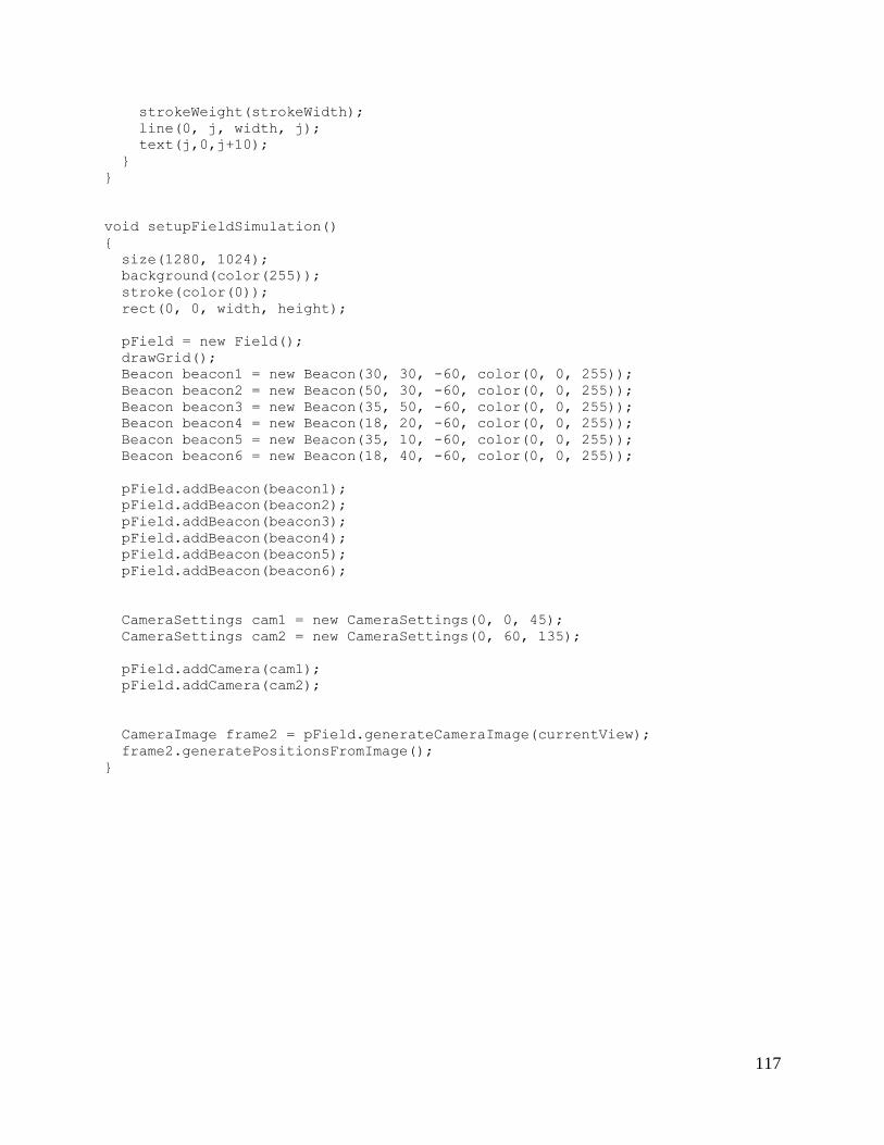
117
strokeWeight(strokeWidth);
line(0, j, width, j);
text(j,0,j+10);
}
}
void setupFieldSimulation()
{
size(1280, 1024);
background(color(255));
stroke(color(0));
rect(0, 0, width, height);
pField = new Field();
drawGrid();
Beacon beacon1 = new Beacon(30, 30, -60, color(0, 0, 255));
Beacon beacon2 = new Beacon(50, 30, -60, color(0, 0, 255));
Beacon beacon3 = new Beacon(35, 50, -60, color(0, 0, 255));
Beacon beacon4 = new Beacon(18, 20, -60, color(0, 0, 255));
Beacon beacon5 = new Beacon(35, 10, -60, color(0, 0, 255));
Beacon beacon6 = new Beacon(18, 40, -60, color(0, 0, 255));
pField.addBeacon(beacon1);
pField.addBeacon(beacon2);
pField.addBeacon(beacon3);
pField.addBeacon(beacon4);
pField.addBeacon(beacon5);
pField.addBeacon(beacon6);
CameraSettings cam1 = new CameraSettings(0, 0, 45);
CameraSettings cam2 = new CameraSettings(0, 60, 135);
pField.addCamera(cam1);
pField.addCamera(cam2);
CameraImage frame2 = pField.generateCameraImage(currentView);
frame2.generatePositionsFromImage();
}

118
Appendix F: List of Materials
This appendix shows the materials we used to implement this system and their individual
costs. These parts were used in every stage of the project and were all used in the final design.