Robotics IFebruary 3, 2017

Exercise 1

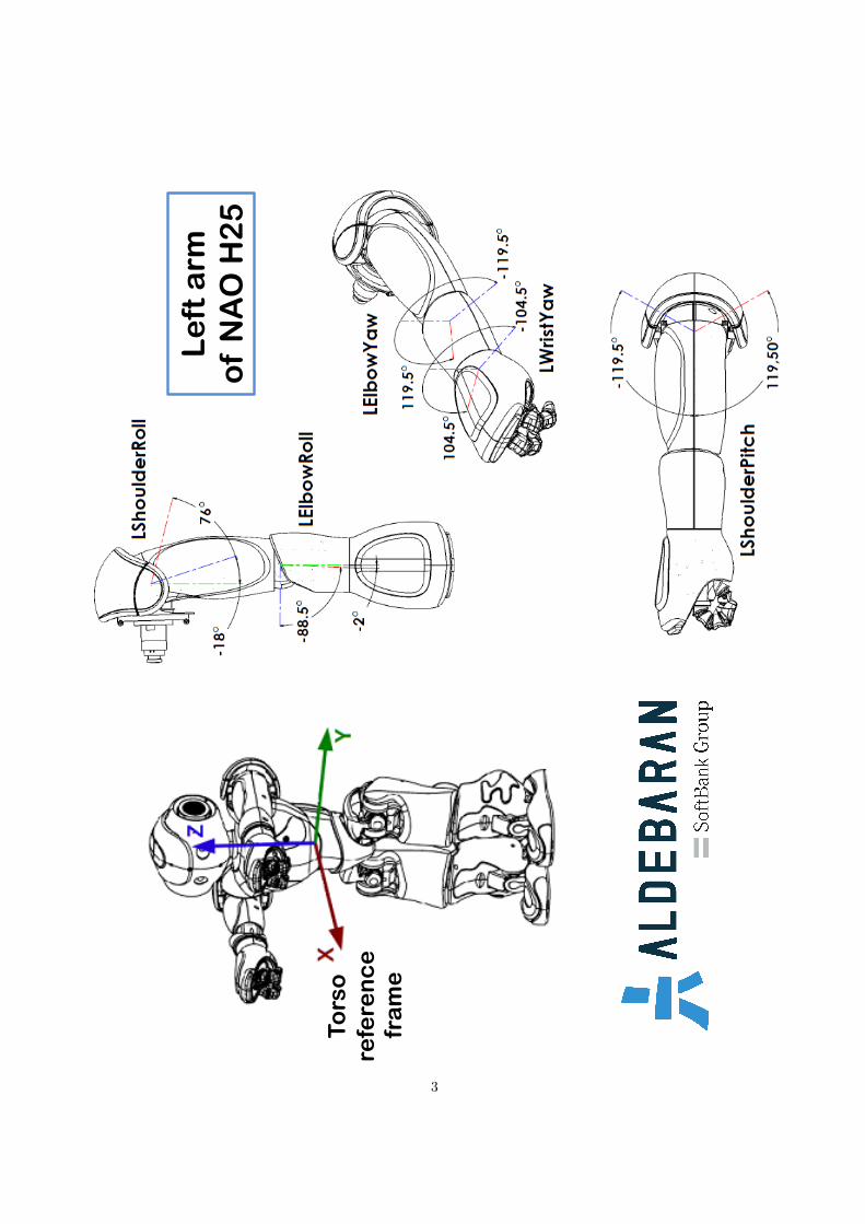
For the NAO humanoid robot in Fig. 1, consider only the left arm down to the wrist yaw joint, whichis frozen together with the remaining joints of all fingers. The left arm has thus four degrees of freedom(dofs). We provide separately a two-sided technical sheet with the kinematic data of this part of the robot.For describing internal motions, the robot has a global reference frame placed at the torso center.

• Assign the reference frames for the first four dofs of the left arm according to the Denavit-Hartenberg(DH) convention, so that the positive senses of joint rotations match those shown in the technical sheet.Place the origin of the last frame at the end of the Lower Arm (i.e., at the Hand base).

• Draw the torso frame (with axes relabeled as xT , yT , and zT ) and the DH frames on one (or on both)of the two distributed extra sheets, which show respectively a CAD view of the torso/left arm and aview of the upper limbs. Provide the 4× 4 homogeneous matrix TA0 from the torso to the DH frame 0.

• Complete the Denavit-Hartenberg table of parameters associated to the frames that have been assigned.

Determine the values of the joint angles q =`q1 q2 q3 q4

´Twhen the robot stretches its left arm

forward and horizontally, just like in the picture on the left of Fig. 1.

Figure 1: The NAO humanoid robot with the torso frame and three views of its left arm.

Exercise 2

For a planar RP robot with direct kinematics and joint velocity/acceleration limits given respectively by

p =

px

py

!=

q2 cos q1

q2 sin q1

!, V max =

2

2.5

![rad/s; m/s], Amax =

3

1.5

![rad/s2; m/s2],

design a minimum time coordinated trajectory, with the end effector moving rest-to-rest between the initial

Cartesian position pi =`

4 3´T

and the final position pf =`−1 1

´T[m].

• Provide the minimum motion time T and draw the velocity/acceleration profiles of the two joints.

• For the given data, will the Cartesian path followed by the end-effector be a linear one? Will the robotpass through a singularity during motion? Prove your responses.

• Compute the (velocity) manipulability measure and sketch a plot of its value during the planned motion.Are there Cartesian positions during this motion in which the force and velocity manipulability ellipsoidswill coincide? Are there configurations at which the velocity ellipsoid becomes a circle? Explain yourresponses and comment on these situations.

1

Exercise 3

A planar 3R robot, having links of equal length `, is being controlled by joint velocity commands q ∈ R3.A desired linear Cartesian trajectory pd(t) is assigned, which starts from point pi at time t = 0 and reachespoint pf at time t = T and has a rest-to-rest motion profile that is continuous for t ∈ [0, T ] up to theacceleration. With reference to Fig. 2, design a single control law for q so that the robot end-effectorposition p = f(q) follows, or at least asymptotically tracks the desired trajectory pd(t). The followingbehaviors should be simultaneously enforced.

1. Realize exact trajectory following (i.e., e(t) = pd(t) − p(t) ≡ 0, ∀t ∈ [0, T ]) for suitable initial configu-rations q(0) = q0,e.

2. For any generic initial configuration q(0) = q0, achieve trajectory tracking with the position error e(t)that converges exponentially to zero.

3. The error component en(t) along the normal direction to the desired linear path should be reduced threetimes faster than the error component et(t) along the tangential direction.

4. Within half of the nominal motion time T/2, the norm of the error ‖e(t)‖ should be reduced at least toone tenth of its initial value.

x0

pi y0

pf

p

Figure 2: A planar 3R robot and a linear Cartesian trajectory.

Use the following numerical data:

` = 2 [m], pi =

4

2

!, pf =

−2

4

![m], T = 4 [s].

• Determine a possible expression of the desired linear Cartesian trajectory pd(t).

• Assuming that kinematic singularities are never encountered, provide the explicit symbolic expressionof all terms in the control law and the proper numerical values of the control gains.

• Find one possible initial configuration q0,e that leads to exact trajectory following, and explain how toobtain such configurations in general.

• When the robot starts from the configuration q0 =`−π/2 0 π/2

´T[rad], compute the numerical

value of the joint velocity command q(0) at the initial time t = 0 with the designed control law.

[240 minutes, open books but no computer or smartphone]

2

Le

ft a

rm

of

NA

O H

25

Tors

o

refe

ren

ce

fr

am

e

3

Fro

nt

vie

w

Top

vie

w

4

Na

me

___

____

____

____

____

____

____

____

____

____

____

____

____

__

5

Na

me

___

____

____

____

____

____

____

____

____

____

____

____

____

__

6

SolutionFebruary 3, 2017

Exercise 1

x2

yT

xT

zT

z0

z1

OT

O2

z2 z3 x1

x3

O4 x4

z4

O3

O0 = O1

x0

Figure 3: The assigned DH frames on a CAD image of the torso and left arm of the NAO.

x2

yT xT

zT

z0

z1

OT

x0 z2

z4

x1

x3

O4

x4

O2 z3

O3

O0 = O1

Figure 4: The assigned DH frames displayed on a picture of the upper limbs of the NAO.

7

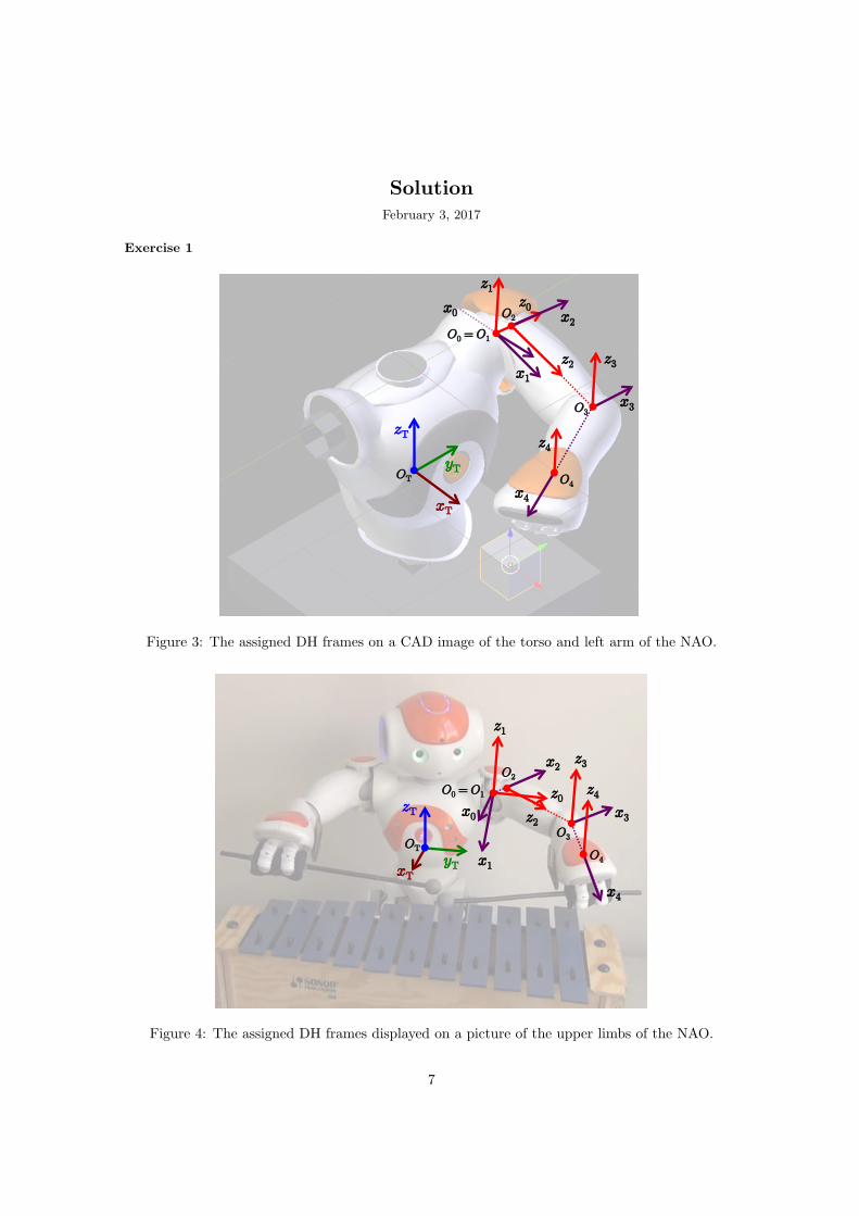
The placement of the torso frame and the Denavit-Hartenberg (DH) assignment for the left arm areillustrated in the two Figs. 3 and 4, for different arm configurations and from different perspective views.The first axis of the shoulder is the ShoulderPitch axis z0, followed by the ShoulderRoll axis z1. Pleasenote the small offset (ElbowOffsetY = 1.5 cm) between the two incident axes at the robot shoulder andthe following axis z2, which provides the ElbowYaw degree of freedom. Without this offset, which wouldthen be added to the value ShoulderOffsetY as a kinematic approximation, the NAO robot would have aspherical shoulder.

x2

x0 x1 O4

x4

xT

z0

yT

x3

O0 = O1

z2

O3

y4

O2

z2

x2 x1

z0 O2 O0 = O1

O3 x3

y3

O4

x4

y4

i !i ai di "i

1 !/2 0 0 q1 = 0

2 !/2 ElbowOffsetY = 15 mm 0 q2 = !/2

3 -!/2 0 UpperArmLength = 105 mm q3 = 0

4 0 LowerArmLength = 55.95 mm 0 q4 = - !/2

yT

zT

z0

z1

OT

x2

O2

O0 = O1 y2

z1

z0 z2

z3 z1 z3 z4

x4

z2

x1

Figure 5: Front and top views of NAO upper limbs with the arms stretched forward and threeviews of the left arm [above]; the DH table of parameters [below].

In Fig. 5, the upper limbs of the NAO are shown from the front and top viewpoints, together with threeviews of the left arm, and the associated DH table is reported. The last column in the table contains the

actual values of the joint variables q =`

0 π/2 0 −π/2´T

when the left arm is stretched forward andhorizontally, as in the picture.

The 4× 4 homogeneous matrix TA0 from the torso frame to the DH frame 0 is given by

TA0 =

0BBBB@1 0 0 0

0 0 1 ShoulderOffsetY

0 −1 0 ShoulderOffsetZ

0 0 0 1

1CCCCA =

0BBBB@1 0 0 0

0 0 1 0.98

0 −1 0 0.10

0 0 0 1

1CCCCA ,

where lengths are expressed in [m].

8

Exercise 2

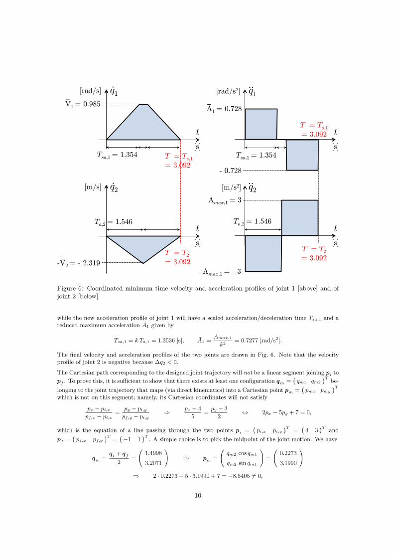
Since the kinematic bounds on motion are imposed on the single joints, it is convenient to plan theinterpolating trajectory in the joint space. The minimum transfer time is achieved when each joint executesa bang-bang or bang-coast-bang acceleration trajectory. Coordinated motion of the robot arm is thenobtained by uniform time scaling of the faster joint(s), so as to align the final time to that of the joint whichhas the slowest completion time (due to the values of the velocity and acceleration limits, in combinationwith the distance to be traveled by that joint).

First, the initial and final Cartesian positions are inverted in the joint space. Considering for simplicityonly the inverse solution for the RP robot which has a positive value for the prismatic variable q2,

p =

px

py

!⇒ q2 =

qp2

x + p2y > 0, q1 = ATAN2{py, px},

we obtain, respectively for p = pi and p = pf ,

qi =

ATAN2{3, 4}√

42 + 32

!=

0.6435

5

!and qf =

ATAN2{1,−1}p

12 + (−1)2

!=

2.3562√

2

![rad; m],

yielding

∆q = qf − qi =

∆q1

∆q2

!=

1.7127

−3.5858

![rad; m].

From the known formula about the existence of a cruising phase in a trapezoidal velocity profile, since

1.7127 = |∆q1| >V 2

max,1

Amax,1=

4

3= 1.3333,

we have that the acceleration profile for the first joint is bang-coast-bang, with acceleration/decelerationtime and minimum transfer time given by

Ta,1 =Vmax,1

Amax,1= 0.6667 [s], T1 =

|∆q1|Amax,1 + V 2max,1

Amax,1 Vmax,1= 1.5230 [s].

On the other hand, since

3.5858 = |∆q2| <V 2

max,2

Amax,2=

9

1.5= 6,

we have that the acceleration profile for the second joint is bang-bang, with acceleration/deceleration time,minimum transfer time, and maximum reached velocity given by

Ta,2 =

p|∆q2|

Amax,2= 1.5461 [s], T2 = 2Ta,2 = 3.0923 [s], V2 =

|∆q2|Ta,2

= 2.3192 [m/s].

Therefore, the minimum time T for the robot motion will be given by the slowest completion time Ti

among all joints (i.e., that of joint 2)

T = max{T1, T2} = 3.0923 [s].

To obtain a coordinated joint trajectory, we need to scale down the motion of joint 1 by the factor

k =T

T1= 2.0304 ⇒ qs,1(t) =

q1(t)

k, qs,1(t) =

q1(t)

k2.

The new trapezoidal velocity profile of joint 1 will have a coordinated motion time Ts,1 and a reducedcruise velocity V1 given by

Ts,1 = k T1 = T = 3.0923 [s], V1 =Vmax,1

k= 0.9850 [rad/s],

9

t

[rad/s]!

V1 = 0.985!

[s]!Tsa,1 = 1.354

q1

T = Ts,1

= 3.092

q1 [rad/s2]!

A1 = 0.728!

T = Ts,1

= 3.092

- 0.728!

t [s]!

Tsa,1 = 1.354

˙ ˙

t

[m/s]!

-V2 = - 2.319!

[s]!

Ta,2 = 1.546

q2

T = T2

= 3.092

q2 [m/s2]!

Amax,1 = 3!

T = T2

= 3.092

t [s]!

Ta,2 = 1.546

˙ ˙

_

_

_

-Amax,1 = - 3!

Figure 6: Coordinated minimum time velocity and acceleration profiles of joint 1 [above] and ofjoint 2 [below].

while the new acceleration profile of joint 1 will have a scaled acceleration/deceleration time Tsa,1 and areduced maximum acceleration A1 given by

Tsa,1 = k Ta,1 = 1.3536 [s], A1 =Amax,1

k2= 0.7277 [rad/s2].

The final velocity and acceleration profiles of the two joints are drawn in Fig. 6. Note that the velocityprofile of joint 2 is negative because ∆q2 < 0.

The Cartesian path corresponding to the designed joint trajectory will not be a linear segment joining pi to

pf . To prove this, it is sufficient to show that there exists at least one configuration qm =`qm1 qm2

´Tbe-

longing to the joint trajectory that maps (via direct kinematics) into a Cartesian point pm =`pmx pmy

´Twhich is not on this segment; namely, its Cartesian coordinates will not satisfy

px − pi,x

pf,x − pi,x=

py − pi,y

pf,y − pi,y⇒ px − 4

5=py − 3

2⇔ 2px − 5py + 7 = 0,

which is the equation of a line passing through the two points pi =`pi,x pi,y

´T=`

4 3´T

and

pf =`pf,x pf,y

´T=`−1 1

´T. A simple choice is to pick the midpoint of the joint motion. We have

qm =qi + qf

2=

1.4998

3.2071

!⇒ pm =

qm2 cos qm1

qm2 sin qm1

!=

0.2273

3.1990

!

⇒ 2 · 0.2273− 5 · 3.1990 + 7 = −8.5405 6= 0,

10

which shows that the Cartesian point is not on the linear path from pi to pf . Moreover, since the analyticJacobian of the RP robot and its determinant are

J(q) =

−q2 sin q1 cos q1

q2 cos q1 sin q1

!⇒ det J(q) = −q2,

and the motion of the second joint is confined between its initial and final values, i.e., q2(t) ∈ˆ√

2, 5˜

forall t ∈ [0, T ], then q2 will never be zero and the robot will not pass through a singularity during motion.

Since the RP robot encounters no singular configurations during motion, the Jacobian will always have

full rank and the identity J#(q)TJ#(q) =

`J(q)JT (q)

´−1holds. Thus, the manipulability ellipsoid in

velocity and the manipulability measure w are given by

vT“J(q)JT (q)

”−1

v = vT

q22 sin2 q1 + cos2 q1

`1− q22

´sin q1 cos q1`

1− q22´

sin q1 cos q1 q22 cos2 q1 + sin2 q1

!v = 1 (1)

and

w =q

det`J(q)JT (q)

´= |q2| .

As a result, during motion the manipulability w will decrease linearly (no need to plot this!) from theinitial value qi,2 = 5 to the final value qf,2 =

√2. On the other hand, by observing the expression of JJT

in (1), we can immediately see that JJT = I for q2 = 1, and the manipulability ellipsoid becomes a circle.In this situation, which is not encountered in this particular planned motion, there is an isotropic behaviorfor the transformation of velocities as well as for the transformation of forces.

Exercise 3

The desired Cartesian trajectory pd(t) can be defined using decomposition in space (tracing a linear path)and time (moving with a quintic polynomial) as

pd(s) = pi + s`pf − pi

´, s ∈ [0, 1], s(t) = 6

„t

T

«5

− 15

„t

T

«4

+ 10

„t

T

«3

, t ∈ [0, T ], (2)

where the six coefficients of a quintic polynomial are necessary and sufficient to impose the required rest-to-rest motion with zero initial velocity and acceleration (which produces a continuous acceleration profilealso at the initial and final instants). The desired Cartesian velocity is then

pd(t) =dpd(s)

dss(t) =

30`pf − pi

´T

„t

T

«4

− 2

„t

T

«3

+

„t

T

«2!. (3)

For later use, we note that the numerical value of pd(t) at the initial time t = 0 is indeed pd(0) = 0.

In view of the requirements, the control problem should be attacked at the Cartesian level. Since the taskis two-dimensional (position tracking in the plane), we consider the following direct kinematics of the 3Rrobot

p = f(q) =

` (c1 + c12 + c123)

` (s1 + s12 + s123)

!, (4)

with the usual shorthand notation, e.g., s123 = sin(q1 + q2 + q3). The associated 2× 3 Jacobian is

J(q) =∂f(q)

∂q=

−` (s1 + s12 + s123) −` (s12 + s123) −` s123` (c1 + c12 + c123) ` (c12 + c123) ` c123

!. (5)

Standard inversion of the non-square Jacobian J is indeed impossible. Rather, we should use the pseu-doinverse J# (or any other form of generalized inversion) in the kinematic control law. Having assumedthat the robot Jacobian remains of full rank during the whole execution of the task, we will evaluate thepseudoinverse as

J#(q) = JT (q)“J(q)JT (q)

”−1

, (6)

11

being JJ# = I.

We remind that a Cartesian kinematic control law of the form

q = J#(q) (pd + Ke) , e(t) = pd(t)− p(t), K > 0, diagonal, (7)

would satisfy most of the problem requirements, except for the specification of the transient error dynamicsalong the tangent and normal directions to the Cartesian path. In fact, when setting K = diag{ki} in thepresent planar case, the error dynamics along the two orthogonal directions x and y would become linearand decoupled, and the two scalar gains ki > 0, i = x, y, in (7) can be chosen so as to yield the desirederror decay, i.e.,

e = pd − p = pd − J(q)q = pd − J(q)J#(q) (pd + Ke) = −Ke ⇒ex = −kxex

ey = −kyey.

However, when using (7), this linear and decoupled dynamics is not displayed along other directions in theplane.

In order to achieve a similar decoupled behavior along the two orthogonal directions xt and yt which are,respectively, tangent and normal to the linear path, we need to rotate the Cartesian error e = 0e into

the task frame attached to the path, react to the rotated error te =`et en

´Tin a decoupled way (so

that the two components of te independently decay at the specified exponential rates), and then map backthis control action into a velocity command expressed in the original Cartesian frame (where the robotJacobian in (5) is also expressed). The kinematic control law (7) becomes then

q = J#(q)“pd + 0Rt K 0RT

t e”, e(t) = pd(t)− p(t), K =

kt 0

0 kn

!> 0, (8)

with the constant 2× 2 (planar) rotation matrix 0Rt defined from the linear path as

xt =pf − pi

‖pf − pi‖=

α

β

!, yt =

−βα

!⇒ 0Rt =

“xt yt

”.

To show the resulting closed-loop behavior, let the rotated error be te = tR00e = 0RT

t0e. Being 0Rt = 0

and using (8), the dynamics of te is

te = tR0 (pd − p) = tR0 (pd − J(q)q) = tR0

“pd − JJ#

“pd + 0Rt K 0RT

t0e””

= −K 0RTt

0e = −K te,

and thuset = −ktet

en = −knen

⇒et(t) = et(0) exp(−ktt)

en(t) = en(0) exp(−knt).

Having set T = 4 [s] for the total motion time, the specification on the transient errors is enforced as follows.Let first kt = kn = k > 0. Being the norm of a vector invariant w.r.t. rotations (

‚‚0e‚‚ =

‚‚0Rtte‚‚ =

‚‚te‚‚),

it is‚‚0e(t)‚‚ =

‚‚te(t)‚‚ =

qe2t (t) + e2n(t) = exp(−kt)

qe2t (0) + e2n(0) = exp(−kt)

‚‚te(0)‚‚ = exp(−kt)

‚‚0e(0)‚‚

Thus, from the requested condition at t = T/2 = 2,‚‚0e(2)‚‚ ≤ 1

10

‚‚0e(0)‚‚ ,

it follows

exp(−2k)‚‚0e(0)

‚‚ ≤ 1

10

‚‚0e(0)‚‚ ⇒ exp(2k) ≥ 10 ⇒ k ≥ 0.5 ln 10 = 1.1513.

12

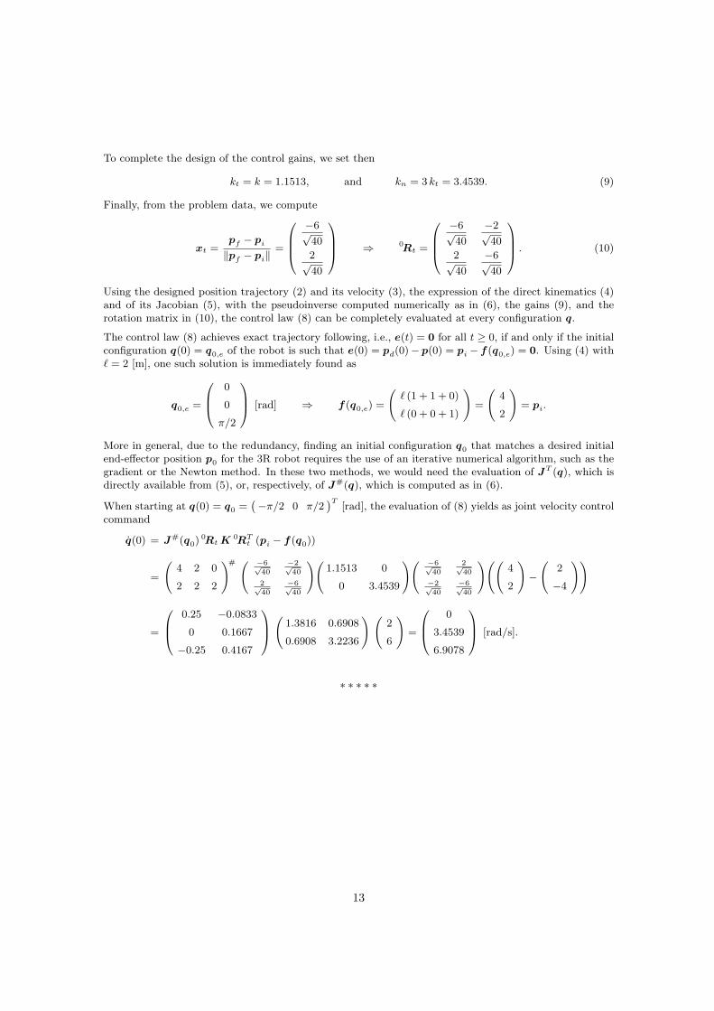
To complete the design of the control gains, we set then

kt = k = 1.1513, and kn = 3 kt = 3.4539. (9)

Finally, from the problem data, we compute

xt =pf − pi

‖pf − pi‖=

0BB@−6√40

2√40

1CCA ⇒ 0Rt =

0BB@−6√

40

−2√40

2√40

−6√40

1CCA . (10)

Using the designed position trajectory (2) and its velocity (3), the expression of the direct kinematics (4)and of its Jacobian (5), with the pseudoinverse computed numerically as in (6), the gains (9), and therotation matrix in (10), the control law (8) can be completely evaluated at every configuration q.

The control law (8) achieves exact trajectory following, i.e., e(t) = 0 for all t ≥ 0, if and only if the initialconfiguration q(0) = q0,e of the robot is such that e(0) = pd(0)− p(0) = pi − f(q0,e) = 0. Using (4) with` = 2 [m], one such solution is immediately found as

q0,e =

0B@ 0

0

π/2

1CA [rad] ⇒ f(q0,e) =

` (1 + 1 + 0)

` (0 + 0 + 1)

!=

4

2

!= pi.

More in general, due to the redundancy, finding an initial configuration q0 that matches a desired initialend-effector position p0 for the 3R robot requires the use of an iterative numerical algorithm, such as thegradient or the Newton method. In these two methods, we would need the evaluation of JT (q), which isdirectly available from (5), or, respectively, of J#(q), which is computed as in (6).

When starting at q(0) = q0 =`−π/2 0 π/2

´T[rad], the evaluation of (8) yields as joint velocity control

command

q(0) = J#(q0) 0Rt K 0RTt (pi − f(q0))

=

4 2 0

2 2 2

!# −6√40

−2√40

2√40

−6√40

! 1.1513 0

0 3.4539

! −6√40

2√40

−2√40

−6√40

! 4

2

!−

2

−4

!!

=

0B@ 0.25 −0.0833

0 0.1667

−0.25 0.4167

1CA 1.3816 0.6908

0.6908 3.2236

! 2

6

!=

0B@ 0

3.4539

6.9078

1CA [rad/s].

∗ ∗ ∗ ∗ ∗

13