robust and adaptive control with aerospace...

Springer Adavanced textbooks in control and Signal Processing

Robust and Adaptive Control with Aerospace Applications

The Solutions Manual

Eugene Lavretsky, Ph.D., Kevin A. Wise, Ph.D.

2/9/2014

The solutions manual covers all theoretical problems from the textbook and discusses several simulation-oriented exercises.

2 Robust and Adaptive Control

Chapter 1

Exercise 1.1. Detailed derivations of the aircraft dynamic modes can be found in many standard flight dynamics textbooks, such as [1]. Further insights can be ob-tained through approximations of these modes and their dynamics using time-scale separation properties of the equations that govern fight dynamics [3].

The time-scale separation concept will now be illustrated. Set control inputs to

zero and change order of the states in (1.7) to: . Then the lon-gitudinal dynamics can be partitioned into two subsystems:

or equivalently,

For most aircraft, their speeds are much greater than the vertical force and moment

sensitivity derivatives due to speed, and so: . Also

and so: . These assumptions are at the core of the time-scale separation principle: The aircraft fast dynamics (the short-period) is almost independent and

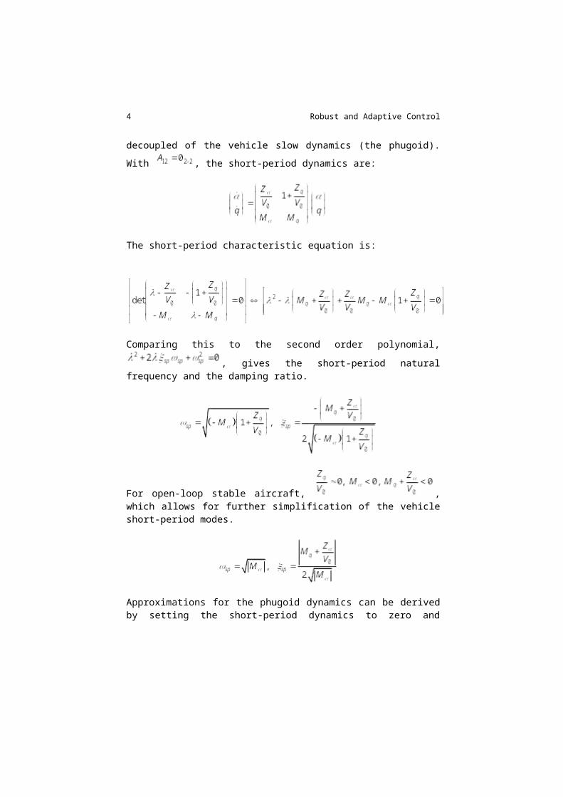
decoupled of the vehicle slow dynamics (the phugoid). With , the short-period dynamics are:

The short-period characteristic equation is:

Comparing this to the second order polynomial, , gives the short-period natural frequency and the damping ratio.

For open-loop stable aircraft, , which allows for further simplification of the vehicle short-period modes.

Approximations for the phugoid dynamics can be derived by setting the short-pe-riod dynamics to zero and computing the remaining modes. This is often referred to as the “residualization of fast dynamics”.

The phugoid dynamics approximation takes the form , or equivalently


Explicit derivations for the phugoid mode natural frequency and damping ratio can be found in [3].

Exercise 1.3. Similar to Exercise 1.1 approach, based on the time-scale separation principle, can also be applied to the lateral-directional dynamics (1.29) to show that the dynamics (1.30) represent the “fast” motion and are comprised of the ve-hicle roll subsidence and the dutch-roll modes. The slow mode (called the “spi-ral”) has the root at the origin. The reader is referred to [1], [2], and [3] for details.

Chapter 2

Exercise 2.1. Same as Example 2.1.

Exercise 2.2. Scalar system is controllable. Use (2.38).

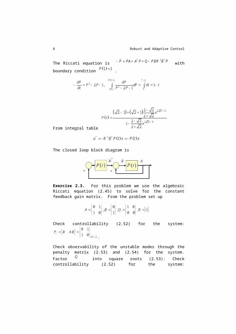
The Riccati equation is with boundary condi-

tion .

From integral table

The closed loop block diagram is

Exercise 2.3. For this problem we use the algebraic Riccati equation (2.45) to solve for the constant feedback gain matrix. From the problem set up

Check controllability (2.52) for the system: .

Check observability of the unstable modes through the penalty matrix (2.53) and (2.54) for the system. Factor into square roots (2.53): Check controllability

(2.52) for the system: . Using (2.54), gives

. Substituting the problem data into the ARE (2.45), yields:

, and therefore:

Exercise 2.4. Use Matlab.

Exercise 2.5. For this problem we use the algebraic Riccati equation (2.45) to solve for the constant feedback gain matrix. From the problem set up


.

Check controllability (2.52) for the system: .

Check observability of the unstable modes through the penalty matrix (2.53) and (2.54) for the system. Factor into square roots (2.53): Check controllability

(2.52) for the system: .

Using (2.54): .

The closed loop system matrix is

Exercise 2.6. . We answer this problem using (2.85). When well posed the LQR problem guarantees a stable closed loop system. When the overall penalty on the states goes to zero. From (2.85)

, so the closed loop poles will be the stable zeros of

, where is the open loop characteristic poly-

nomial. If any open loop poles in are unstable, they are stable in .

When the overall penalty on the control goes to zero. This creates a high gain situation. From (2.89), some of the roots will go to infinity along asymptotes. Those that stay finite will approach the stable transmission zeros of the transfer

function matrix . These finite zeros shaped by the matrix control the dy-namic response of the optimal regulator.

Exercise 2.7. 1) The HJ equation is . Substitut-ing the system data into the equation, gives

. Substitute this back into to form .

,

with boundary conditions .

2) If we try then

. Substitute back into the HJ equation.


Group terms:

.

We want this to hold for all . Get three equations inside the parentheses. To

solve for the boundary conditions, expand and equate coefficients.

Chapter 3

Exercise 3.1. a) The suspended ball plant model is . The

open loop eigenvalues are: , Since the model is in controllable canonic form, we see that it is controllable. The state feedback con-trol law is which has two elements in the gain matrix. The closed loop

system using the state feedback control is .

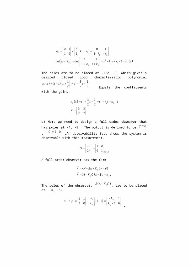
The poles are to be placed at -1/2, -1, which gives a desired closed loop character-

istic polynomial . Equate the coefficients with the gains:

b) Here we need to design a full order observer that has poles at -4, -5. The output

is defined to be . .An observability test shows the system is ob-servable with this measurement.

A full order observer has the form

The poles of the observer, , are to be placed at -4, -5.

.

Using observer feedback for the control , yields


where , . Connecting the plant and controller to form the extended closed loop system, gives

Substituting the matrices to form , results in

.

c) For the reduced order observer, we will implement a Luenberger design that has

the form . Choose the matrix to make the matrix

nonsingular. Define . Then the reduced order observer matrices and control law are given by:

Where is the reduced order observer gain matrix. First we need :

Substituting into the observer matrices yields

The problem asks to place the observer pole at -6. Thus which gives

and . So, . To form the state estimate we

use . The control is where is computed from part c).

To form the controller as a single transfer function, take the Laplace transform and combine the above expressions. The block diagram showing the plant and con-troller is

B-

1sI A C

21 12

152

s

s

u1y x

Exercise 3.2. Use file Chapter3_Example3p5.m to solve this problem.



Chapter 4




Chapter 5

Exercise 5.1. The following code will complete the problem:

% Set up frequency vector


w = logspace(-3,3,500);

% Loop through each frequency and compute the det[I+KH]

% The controller is a constant matrix so keep it out-side the loop

K = [ 5. 0.

0. -10. ];

x_mnt = zeros(size(w));% pre-allocate for speed

x_rd = zeros(size(w));

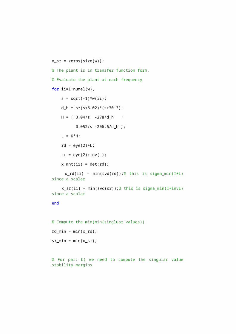
x_sr = zeros(size(w));

% The plant is in transfer function form.

% Evaluate the plant at each frequency

for ii=1:numel(w),

s = sqrt(-1)*w(ii);

d_h = s*(s+6.02)*(s+30.3);

H = [ 3.04/s -278/d_h ;

0.052/s -206.6/d_h ];

L = K*H;

rd = eye(2)+L;

sr = eye(2)+inv(L);

x_mnt(ii) = det(rd);

x_rd(ii) = min(svd(rd));% this is sigma_min(I+L) since a scalar

x_sr(ii) = min(svd(sr));% this is sigma_min(I+invL) since a scalar

end

% Compute the min(min(singluar values))

rd_min = min(x_rd);

sr_min = min(x_sr);

% For part b) we need to compute the singular value stability margins

neg_gm = 20*log10( min([ (1/(1+rd_min)) (1-sr_min)])); % in dB

pos_gm = 20*log10( max([ (1/(1-rd_min)) (1+sr_min)])); % in dB

pm = 180*(min([2*asin(rd_min/2) 2*asin(sr_min/2)]))/pi;% in deg

To plot the multivariable Nyquist results, plot the real and imaginary components of x_mnt and count encirclements.

-3 -2 -1 0 1 2 3-3

-2

-1

0

1

2

3

Real

Imag

MNT Problem 5.1a

We see no encirclements.

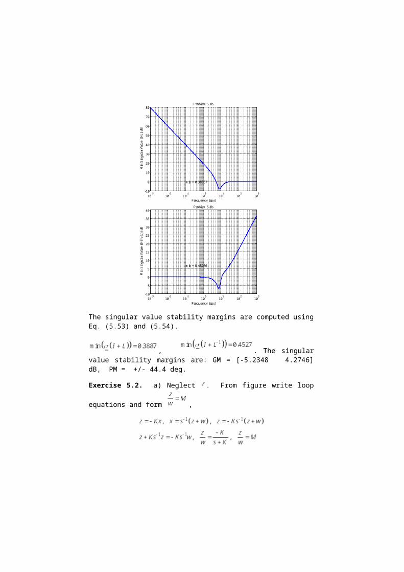
b) Plot the minimum singular values of and versus frequency, con-verting to dB.


10-3

10-2

10-1

100

101

102

103

-10

0

10

20

30

40

50

60

70

80

Frequency (rps)

Min

Sin

gula

r Va

lue

(I+L

) dB

Problem 5.1b

min = 0.38867

10-3

10-2

10-1

100

101

102

103

-10

-5

0

5

10

15

20

25

30

35

40

Frequency (rps)

Min

Sin

gula

r Va

lue

(I+i

nv(L

)) d

B

Problem 5.1b

min = 0.45266

The singular value stability margins are computed using Eq. (5.53) and (5.54).

, . The singular value stabil-ity margins are: GM = [-5.2348 4.2746] dB, PM = +/- 44.4 deg.

Exercise 5.2. a) Neglect . From figure write loop equations

and form ,

where should be the negative of the closed loop transfer func-tion at the plant input loop break point. The state space model is

not unique. Here we choose

.

b) For stability we need the pole in the transfer function to be stable. Thus .

c) From equation (5.92) we plot :

0 dB

Mag

w

Breaks at w = 1 r/s

d) The small gain theorem (5.92) says that . The above plot

shows that as long as this will be satisfied. If we compute the closed loop transfer function from command to output in problem figure i), we have

As long as , the uncertainty cannot create a negative coefficient on the gain in the denominator.

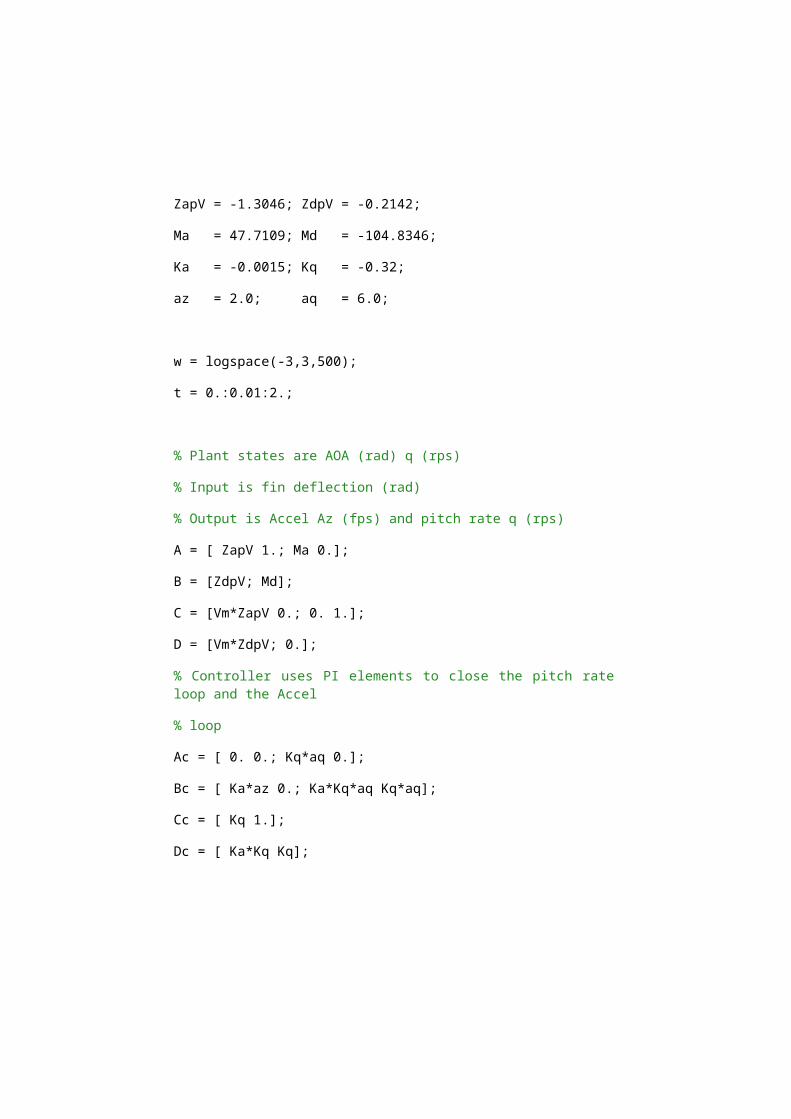
Exercise 5.3. a) Populate the problem data into the plant (5.8) and controller (5.18). Then use (1.42) to form the closed loop system.

% Pitch Dynamics

Vm = 886.78;

ZapV = -1.3046; ZdpV = -0.2142;

Ma = 47.7109; Md = -104.8346;

Ka = -0.0015; Kq = -0.32;

az = 2.0; aq = 6.0;


w = logspace(-3,3,500);

t = 0.:0.01:2.;

% Plant states are AOA (rad) q (rps)

% Input is fin deflection (rad)

% Output is Accel Az (fps) and pitch rate q (rps)

A = [ ZapV 1.; Ma 0.];

B = [ZdpV; Md];

C = [Vm*ZapV 0.; 0. 1.];

D = [Vm*ZdpV; 0.];

% Controller uses PI elements to close the pitch rate loop and the Accel

% loop

Ac = [ 0. 0.; Kq*aq 0.];

Bc = [ Ka*az 0.; Ka*Kq*aq Kq*aq];

Cc = [ Kq 1.];

Dc = [ Ka*Kq Kq];

% Form closed loop system

[kl,kl]=size(D*Dc); Z=inv(eye(kl)+D*Dc);

[kl,kl]=size(Dc*Z*D);EE=eye(kl)-Dc*Z*D;

[kl,kl]=size(Z*D*Dc);FF=eye(kl)-Z*D*Dc;

Acl=[(A-B*Dc*Z*C) (B*EE*Cc);

(-Bc*Z*C) (Ac-Bc*Z*D*Cc)];

Bcl=[(B*EE*Dc);

(Bc*FF)];

Ccl = [(Z*C) (Z*D*Cc)];

Dcl=(Z*D*Dc);

% Step Response

y=step(Acl,Bcl,Ccl,Dcl,1,t);

az = y(:,1);

q = y(:,2);


0 0.5 1 1.5 2-0.2

0

0.2

0.4

0.6

0.8

1

1.2

Time (sec)

Acc

el A

z (fp

s)

Problem 5.3 Accel Step Response

Rise Time = 0.39

Settling Time = 0.95

0 0.5 1 1.5 2-2

-1.8

-1.6

-1.4

-1.2

-1

-0.8

-0.6

-0.4

-0.2

0x 10

-3

Time (sec)

Pitc

h R

ate

q (r

ps)

Problem 5.3 Accel Step Response

b)

% Break the loop at the plant input

A_L = [ A 0.*B*Cc; -Bc*C Ac];

B_L = [ B; Bc*D];

C_L = -[ -Dc*C Cc]; % change sign for loop gain

D_L = -[ -Dc*D];

theta = pi:.01:3*pi/2;

x1=cos(theta);y1=sin(theta);

[re,im]=nyquist(A_L,B_L,C_L,D_L,1,w);

L = re + sqrt(-1)*im;

rd_min = min(abs(ones(size(L))+L));

sr_min = min(abs(ones(size(L))+ones(size(L))./L));

-3 -2 -1 0 1 2 3-3

-2

-1

0

1

2

3Problem 5.3 Nyquist

Real

Imag

inar

y

-5 0 5-5

-4

-3

-2

-1

0

1

2

3

4

5Problem 5.3 Nyquist

Real

Imag

inar

y


10-3

10-2

10-1

100

101

102

103

-20

0

20

40

60

80

100

120

140

160

0.90921

Problem 5.3 Return Difference I+L

Frequency (rad/s)

Mag

nitu

de (

dB)

10-3

10-2

10-1

100

101

102

103

-5

0

5

10

15

20

0.75411

Problem 5.3 Stability Robustness I+INV(L)

Frequency (rad/s)

Mag

nitu

de (

dB)

The singular value stability margins are computed using Eq. (5.53) and (5.54).

% Compute singluar value margins

neg_gm = 20*log10( min([ (1/(1+rd_min)) (1-sr_min)])); % in dB

pos_gm = 20*log10( max([ (1/(1-rd_min)) (1+sr_min)])); % in dB

pm = 180*(min([2*asin(rd_min/2) 2*asin(sr_min/2)]))/pi;% in deg

Min Singular value I+L = 0.90921. Min Singular value I+inv(L) = 0.75411. Sin-gular value gain margins = [-12.1852 dB, +20.8393 dB ]. Singular value phase margins = +/-44.3027 deg.

c) From Figure 5.23, we want to model the actuator using an uncertainty model at

the plant input : . Note that we have a negative sign on the summer, which is different from Figure 5.23. The modified block diagram would be:

+

-

+1

+K G

1z 1w

The problem requires to model the actuator using a first order transfer function

. We equate these and solve for the uncertainty:

d) Form the analysis model where the uncertainty is from part c). The matrix from (5.70) can be easily modified here (due to the negative feedback). It is derived as follows:

e) Here we pick a time constant for the actuator transfer function in part c) and

plot . For this problem , since is a scalar, and we can reuse the result from b).


10-3

10-2

10-1

100

101

102

103

-120

-100

-80

-60

-40

-20

0

20

Frequency (rad/s)

Mag

nitu

de (

dB)

Problem 5.3 SGT Actuator Analysis)

I+invL min = 0.75411tau = 0.005 stau = 0.02 stau = 0.08 s

From the figure we see that an actuator with time constant of 0.08 sec overlaps (red curve).

Exercise 5.4. Matlab code from example 5.2 can be used here. The Bode plots:

10-3

10-2

10-1

100

101

102

103

-40

-20

0

20

40

60

80

Frequency (rad/s)

Mag

nitu

de (

dB)

Problem 5.4 Bode

10-3

10-2

10-1

100

101

102

103

-280

-260

-240

-220

-200

-180

-160

-140

-120

-100

-80

Frequency (rad/s)

Pha

se (

deg)

Problem 5.4 Bode

The Nyquist curve:

-3 -2 -1 0 1 2 3-3

-2

-1

0

1

2

3

Real

Imag

Problem 5.4 Nyquist

10-3

10-2

10-1

100

101

102

103

0

10

20

30

40

50

60

70

80

1

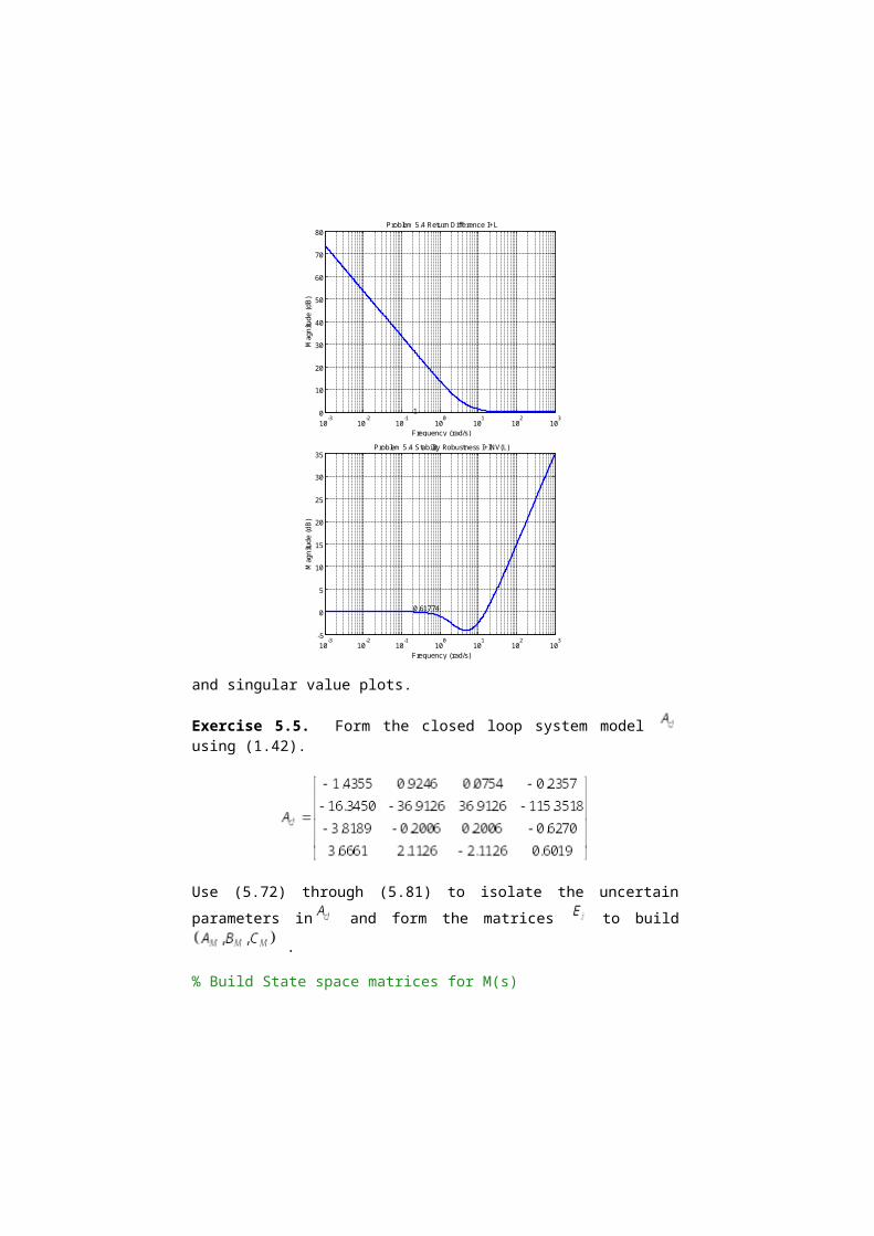
Problem 5.4 Return Difference I+L

Frequency (rad/s)

Mag

nitu

de (

dB)

10-3

10-2

10-1

100

101

102

103

-5

0

5

10

15

20

25

30

35

0.61774

Problem 5.4 Stability Robustness I+INV(L)

Frequency (rad/s)

Mag

nitu

de (

dB)

and singular value plots.


Exercise 5.5. Form the closed loop system model using (1.42).

Use (5.72) through (5.81) to isolate the uncertain parameters in and form the matrices to build .

% Build State space matrices for M(s)

[nxcl,~]=size(Acl);

E1 = 0.*ones(nxcl,nxcl);

E1(:,1) = Acl(:,1);

E1(2,1) = 0.;

E1(3,1) = 0.;

[U1,P1,V1]=svd(E1);

b1=sqrt(P1(1,1))*U1(:,1);

a1=sqrt(P1(1,1))*V1(:,1).';


E2(:,3) = Acl(:,3);

E2(2,3) = 0.;

E2(3,3) = 0.;

[U2,P2,V2]=svd(E2);

b2=sqrt(P2(1,1))*U2(:,1);

a2=sqrt(P2(1,1))*V2(:,1).';


E3(2,1) = Acl(2,1);

[U3,P3,V3]=svd(E3);

b3=sqrt(P3(1,1))*U3(:,1);

a3=sqrt(P3(1,1))*V3(:,1).';


E4(2,3) = Acl(2,3);

[U4,P4,V4]=svd(E4);

b4=sqrt(P4(1,1))*U4(:,1);

a4=sqrt(P4(1,1))*V4(:,1).';

% M(s) = Cm inv(sI - Am) Bm

Am=Acl;

Bm=[b1 b2 b3 b4];

Cm=[a1;a2;a3;a4];

Using the model for compute the structure singular value and the small

gain theorem bound. Extract the minimum value of and .


10-1

100

101

102

-30

-20

-10

0

10

20

30

40

50

60

Frequency (rps)

1/m

u an

d 1/

sigm

(M) d

B

Delta = Diagonal Real Matrix

min(1/mu) = 0.65242min(1/sigma(M)) = 0.085765

Chapter 6

Exercise 6.1. Use file Chapter6_Example6p1_rev.m to solve this problem.



Chapter 7

Exercise 7.2. Substituting the adaptive controller

and the reference model into the open-loop roll dynam-

ics , gives the closed-loop system (7.28). To derive (7.29), use

in the error dynamics (7.18), and in the adaptive laws (7.24). Since the system unknown parameters are assumed to be constant, the second and the

third equations in (7.29) immediately follow. The stabilization solution (7.30) is a special case of (7.28) when the external command is set to zero.

Chapter 8

Exercise 8.2. The trajectories of , starting at , can be de-rived by direct integration of the system dynamics on time intervals where the

sign of remains constant: .

Suppose that for some . Then equating the left hand side of the tra-

jectory equation to zero, gives . Multiplying both sides by

, results in , and so , which implies that any

two solutions with the same value of become zero at the same time . Fi-nally, it is evident that all solutions are discontinuous at any instant in time

when , and thus the solutions are not continuously differentiable.

Exercise 8.3. Rewrite the system dynamics as . Since

then , and consequently

is the system unique trajectory, with the initial condition

. The system phase portrait is easy to draw. It represents a monotoni-

cally strictly increasing cubic polynomial . These dynamics are lo-

cally Lipschitz. Indeed, since

then , for any with , where is a finite positive constant, that is the system dynamics are locally Lip-

schitz. However, the dynamics are not globally Lipschitz since is unbounded.


Exercise 8.4. Suppose that the scalar autonomous system has a unique

non-monotonic trajectory . Then there must exist a finite time instant

where . Therefore for all , is constant, which in turn contradicts the argument of the trajectory being non-monotonic.

Exercise 8.5. If then the system has the unique isolated equi-

librium . Otherwise, the equilibrium set of the system is de-

fined by the linear manifold , implying an infinite number of solutions.

Exercise 8.6. Trajectories of the scalar non-autonomous system with

the initial condition can be written as . The

system equilibrium point is . Suppose that is continuous in time. In order to prove stability in the sense of Lyapunov, one needs to show that for any

there exists such that for all . Based on the explicit form of the solution, it is easy to see that boundedness of the system

trajectories is assured if and only if . In this

case, it is sufficient to select . If then as-

ymptotic stability takes place. If in addition, is bounded as a function of

then can be chosen independent of and the asymptotic stability becomes uniform.

Exercise 8.7. Since then

This proves global positive definiteness of . Clearly , and so

is also radially unbounded. Differentiating along the system trajecto-ries, gives:

So, is a Lyapunov function and the origin is globally uniformly stable. To

prove asymptotic stability, consider the set of points where

. On this set . If a trajectory gets “trapped” in then .

Outside of the set, and consequently trajectories enter and then go to the origin. These dynamics can also be explained using LaSalle’s Invariance Prin-ciple [2] for autonomous systems. The principle claims that the system trajectories will approach the largest invariant set in . Here, this set contains only one point – the origin. The overall argument proves global asymptotic uniform stability of the system equilibrium.

Exercise 8.8. Due to the presence of the sign function, the system dynamics are discontinuous in and thus, sufficient conditions for existence and uniqueness do not apply. However, the system solutions can be defined in the sense of Filippov [2]. This leads to the notion of the “sliding modes” in dynamical systems. Con-

sider the manifold , whose dynamics along the system trajectories are:

In Exercise 8.2, the same exact dynamics were considered. It was shown that start-

ing from any initial conditions, the system trajectories reach zero in finite

time. In terms of the original system, it means that the system state reaches

the linear manifold in finite time. On the manifold ,


and so , which in itself implies that after reaching the manifold, the trajec-tories “slide” down to the origin.

Exercise 8.9. Let represent a scalar continuously differentiable

function whose derivative is bounded: . Then for any and there

exists such that

and so , for any . This proves uniform conti-

nuity of on .

We now turn our attention to proving Corollary 8. 1, where by the assumption, a

scalar function is twice continuously differentiable, with bounded second

derivative . Therefore, the function first derivative is uniformly con-

tinuous. In addition, it is assumed that has a finite limit, as . Then

due to Barbalat’s Lemma, tends to zero, which proves the corollary.

Exercise 8.10. Substituting into the system dynamics, gives

where is Hurwitz, and is the feedback gain estimation error. The

desired reference dynamics are . Subtracting the latter from

the system dynamics, results in , with the state tracking error

. Also, the feedback gain dynamics can be written as . For the closed-loop system error system,

consider a Lyapunov function candidate . Clearly, this function is positive definite and radially unbounded. Its derivative along the closed-loop system error dynamics is

This proves: a) Uniform stability of the system error dynamics; and b) Uniform

boundedness of the system errors, that is . Since the external input

is bounded then , and so is . Then and consequently, the error and the state derivatives are uniformly bounded as well,

. Since then is a uniformly continuous function of time. Note that is lower bounded and its time derivative is non-positive. Hence, tends to a limit, as a function of time. Using Barbalat’s

Lemma, we conclude that , which is equivalent to

. The latter proves bounded asymptotic command tracking ability of

the controller, that is , for any bounded external command .

Consequently, . Finally, if then the DC gain of the reference model is unity. In this case, both the system state

and the reference model state will asymptotically track any external bounded command with zero steady-state errors.

Chapter 9

Exercise 9.1. Let some of the diagonal elements of in the system dynamics (9.40) be negative and assume that the signs of them are known. Consider the modified Lyapunov function (9.43),


where denotes the diagonal matrix with positive elements . It is easy to see that this function is positive definite and radially unbounded. Let

. Then . Repeating derivations

(9.55) through (9.58) with in place of , gives the modified adaptive laws.

Chapter 10

Exercise 10.1. We need to prove that

with a Hurwitz matrix and

So, , where “ ” indicates “do not care” elements. Denote

where are of the corresponding dimensions. Then

and thus . Finally,

and so, the reference model DC gain is unity.

Exercise 10.2. Starting with the adaptive controller , the

adaptive law is initialized at the baseline gain values

. Then

where represents an adaptive incremental gain whose adaptive law dynamics

are the same as for the original adaptive gain . The resulting total control input,

represents an adaptive augmentation of a baseline linear controller .

Exercise 10.3. Consider the error dynamics and

assume that the extended regressor is continuously differentiable in its arguments. Then

The first term in the right hand side of the equation is uniformly bounded. Also,

all the functions in the second term are uniformly bounded. Therefore

and is a uniformly continuous function of time. Since in addition tends


to zero then using Barbalat’s Lemma we conclude that tends to zero as well.

Then the error dynamics imply: .

Chapter 11

Exercise 11.1. The Projection Operator, as defined in (11.37), is continuous and differentiable in its arguments. Consequently, it is locally Lipschitz.

Exercise 11.3. Since

it is sufficient to show that . By the assumption,

. Then

The above inequality allows one to use the adaptive laws (11.53) and carry out the proof of the system UUB properties, while repeating the exact same arguments as in Section 11.5.

Chapter 12

Exercise 12.2. There are several ways to embed a baseline linear controller into the overall design and then turn the adaptive system from Table 12.1 to act as an

augmentation to the selected baseline controller. Our preferred way to perform such a design starts with the assumed open-loop system linear dynamics without

the uncertainties. A robust linear feedback controller can be designed for the linear system. Then the corresponding closed-loop linear system dynamics become the reference model for the adaptive system to achieve and maintain in the presence of uncertainties. So in (12.14), the reference model matri-

ces are defined as the closed-loop linear system matrices achieved un-der the selected linear baseline controller. The total control input is defined similar to (12.16)

Repeating the derivations from Section 10.3, the open-loop system with the imbedded baseline controller becomes very similar to (10.47, 10.48). In this case, the adaptive component will depend on the baseline controller, as shown in (10.51). Starting from (12.24) and repeating the same design steps will result in adaptive laws similar to (12.37). The only difference here will be in the addition of adaptive dynamics on the baseline gains, as shown in (10.66).

Alternatively, one can choose to initialize the adaptive gains at the corre-

sponding gain values of the selected baseline controller, and then use the arguments from Exercise 10.2 to justify the design. However, in practical ap-plications this approach may result in unnecessary numerical complications if the gains of the baseline controller are scheduled to depend on the system slowly time-varying parameters.

Exercise 12.4. First, set and design a base-

line linear feedback controller in the form for the assumed nominal linear open-loop dynamics. Note, that due to the inclusion of the integrated output tracking error system into the design, the baseline linear controller has “classical”

(Proportional + Integral) feedback connections: .

Second, form the reference system to represent the closed-loop baseline linear dy-namics with the embedded baseline linear controller.


Third, define the total control input without the adaptive component on the exter-nal command.

Finally, follow the rational from Exercise 12.2, and repeat the design steps from Section 12.4, starting with the modified controller definition.

Chapter 13

Exercise 13.1. Differentiating the error dynamics (13.5), gives

If is uniformly bounded in time then , since it has already been proven that all signals in the right hand side of the above equation are uni-

formly bounded. Therefore, is a uniformly continuous function of time. Also

it was proven that . Using Barbalat’s Lemma, implies ,

and so, the signal in the error dynamics (13.5),

must asymptotically tend to zero.

Exercise 13.2. Consider the system (13.31).

with Hurwitz . The system solution is:

From an engineering perspective, these dynamics can be viewed as a linear stable

filter with as the input. So, if the latter decays to zero then the state of the filter will do the same. This argument can also be proven formally using the control-theoretic arguments from the given reference.

Exercise 13.3. Use the results from Exercise 13.1. In this case, the error dynamics

(13.101) does not explicitly depend on the external command . Without assuming continuity or even differentiability of the latter, one can differentiate the

error dynamics (13.101), show that and then repeat the arguments from

Exercise 13.1 to prove that .

Chapter 14

Exercise 14.1. Suppose that all states are accessible, i.e., . Disregarding the Projection Operator, the output feedback (baseline + adaptive) control input, the adaptive laws, and the corresponding reference model (aka, the state observer) become (see Table 14.1):

At the same time, a state feedback MRAC system can be written as, (see Table 10.2):


Clearly, the main difference between the two systems is in the use of the state ob-server for the former, as oppose to the “ideal” reference model for the latter. An-other difference consists of employing the estimated / filtered state feedback in the observer-based adaptive system versus the original system state feedback in MRAC. As it was formally shown in Chapters 13 and 14, these two design fea-tures give the observer-based adaptive system a distinct advantage over the classi-cal MRAC: It is the ability to suppress undesirable transients.

Exercise 14.2. Instead of using (14.14), consider the original dynamics (14.7)

and the state observer,

where are the parameters to be estimated. Choosing the control input,

gives the linear state observer dynamics.

Subtracting the observer form the system, results in the observer error dynamics,

which are very similar to (14.24). Repeating all the design steps after (14.24) will result in the pure (no baseline included) adaptive laws alike (14.47).

with . The rest of the design steps mirror the ones in Section 14.4.

Exercise 14.3. For the open-loop system,

with an unknown strictly positive definite diagonal matrix , there exists a control input in the form

with unknown gains and that would have resulted in the desired closed-loop stable reference dynamics,

where are the two known matrices that define the desired closed-loop dynamics. This is an existence-type statement. Its validity is predicated on the fact

that the pair is controllable and the two desired matrices are chosen to sat-

isfy the Matching Conditions (MC): . The MC impose restrictions on the selection of achievable dynamics for the original sys-tem, which in turn can be rewritten as:


where denotes the aggregated set of unknown parame-ters in the system. With that in mind, consider the state observer

where is the vector of to-be-estimated parameters. Choosing,

yields the linear time-invariant state observer dynamics.

With the state and output errors defined as in (14.23),

the observer error dynamics

are in the form of (14.24), with in place of and instead of . Repeat-ing the arguments starting from (14.24) will give stable output feedback observer-based adaptive laws in the form of (14.47),

along with the associated proofs of stability and bounded tracking performance.

robust and adaptive control with aerospace...

Documents