robust and lpv control of mimo systems part 2: h controlo.sename/docs/hinfcontrol.pdf · robust and...

Robust and LPV control of MIMO systemsPart 2: H∞ control

Olivier Sename

GIPSA-Lab

Tecnologico de Monterrey, July 2016

Olivier Sename (GIPSA-Lab) Robust and LPV control - part 2 Tecnologico de Monterrey, July 2016 1 / 47

1. What is theH∞ performance?TheH∞ norm definitionH∞ norm as a measure of the system gain ?How to compute theH∞ norm?

2. What isH∞ control?

3. How to solve an H∞ control problem?The Static State feedback caseThe Dynamic Output feedback caseThe Riccati approachThe LMI approach forH∞ control design

4. WhyH∞ control is adapted to control engineering?Performance analysis using the sensitivity functionsPerformance specifications in view ofH∞ control design

SISO caseMIMO case

The mixed sensitivityH∞ control design

O. Sename [GIPSA-lab] 2/47

What is theH∞ performance? TheH∞ norm definition

H∞ norm

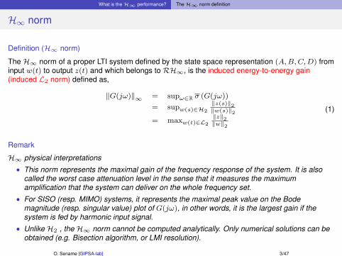
Definition (H∞ norm)

The H∞ norm of a proper LTI system defined by the state space representation (A,B,C,D) frominput w(t) to output z(t) and which belongs to RH∞, is the induced energy-to-energy gain(induced L2 norm) defined as,

‖G(jω)‖∞ = supω∈R σ (G(jω))

= supw(s)∈H2

‖z(s)‖2‖w(s)‖2

= maxw(t)∈L2

‖z‖2‖w‖2

(1)

Remark

H∞ physical interpretations• This norm represents the maximal gain of the frequency response of the system. It is also

called the worst case attenuation level in the sense that it measures the maximumamplification that the system can deliver on the whole frequency set.

• For SISO (resp. MIMO) systems, it represents the maximal peak value on the Bodemagnitude (resp. singular value) plot of G(jω), in other words, it is the largest gain if thesystem is fed by harmonic input signal.

• Unlike H2 , the H∞ norm cannot be computed analytically. Only numerical solutions can beobtained (e.g. Bisection algorithm, or LMI resolution).


What is theH∞ performance? H∞ norm

Illustration

For a SISO system, z = Gd, the gain at a given frequency is simply

|z(ω)||d(ω)|

=|G(jω)d(ω)||d(ω)|

= |G(jω)|

The gain depends on the frequency, but since the system is linear it is independent of the inputmagnitudeFor a MIMO system we may select:

‖z(ω)‖2‖d(ω)‖2

=‖G(jω)d(ω)‖2‖d(ω)‖2

= ‖G(jω)‖2

Which is "independent" of the input magnitude. But this is not a correct definition. Indeed the inputdirection is of great importance



A first ’bad’ approach

Let consider

G =

[5 43 2

]How to define and evaluate its gain ?Consider five different inputs:

d =

(10

)d =

(01

)d =

(0.7070.707

)d =

(0.707−0.707

)d =

(0.6−0.8

)Input magnitude :

‖d1‖2 = ‖d2‖2 = ‖d3‖2 = ‖d4‖2 = ‖d5‖2 = 1

But the corresponding outputs are

z =

(53

)z =

(42

)z =

(6.36303.5350

)z =

(0.70700.7070

)z =

(−0.20.2

)and

the ratio are ‖z‖2/‖d‖25.8310 4.4721 7.2790 0.9998 0.2828



Towards SVD


MAXIMUM SINGULAR VALUE

maxd 6=0

‖Gd‖2‖d‖2

= σ(G)

MINIMUM SINGULAR VALUE

mind 6=0

‖Gd‖2‖d‖2

= σ(G)

We see that, depending on the ratiod20/d10, the gain varies between 0.27and 7.34 .


What about eigenvalues ?

Eigenvalues are a poor measure of gain. Let

G =

[0 1000 0

]Eigenvalues are 0 and 0.But an input vector [

01

]leads to an output vector [

1000

].

Clearly the gain is not zero.Now, the maximal singular value is = 100It means that any signal can be amplified at most 100 timesThis is the good gain notion.



Characterization of the H∞ norm as induced L2 norm

Finally, in the case of a transfer matrix G(s) : (m inputs, p outputs) u vector of inputs, y vector ofoutputs.

σ(G(jω)) ≤‖z(ω)‖2‖d(ω)‖2

≤ σ(G(jω))


Example of A two-mass/spring/damper system2 inputs: F1 and F2 2 outputs: x1 and x2

Singular Values

Frequency (rad/sec)S

ingu

lar V

alue

s (d

B)

10-1

100

101

102

-100

-80

-60

-40

-20

0

20

40

Hinf norm 11.4664 = 21.18 dB

smallest singular value

largest singular value

G=ss(A,B,C,D): LTI systemnormhinf(G): Compute Hinf normnorm(G,inf): Compute Hinf normsigma(G): plot max and min SV

What is theH∞ performance? H∞ norm computation

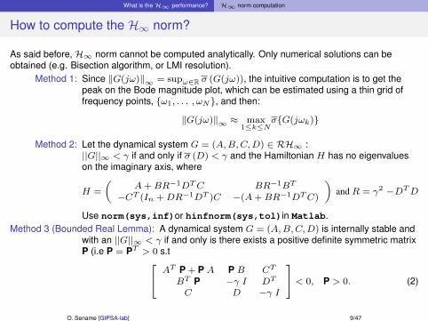
How to compute the H∞ norm?

As said before, H∞ norm cannot be computed analytically. Only numerical solutions can beobtained (e.g. Bisection algorithm, or LMI resolution).

Method 1: Since ‖G(jω)‖∞ = supω∈R σ (G(jω)), the intuitive computation is to get thepeak on the Bode magnitude plot, which can be estimated using a thin grid offrequency points, {ω1, . . . , ωN}, and then:

‖G(jω)‖∞ ≈ max1≤k≤N

σ{G(jωk)}

Method 2: Let the dynamical system G = (A,B,C,D) ∈ RH∞ :||G||∞ < γ if and only if σ (D) < γ and the Hamiltonian H has no eigenvalueson the imaginary axis, where

H =

(A+BR−1DTC BR−1BT

−CT (In +DR−1DT )C −(A+BR−1DTC)

)and R = γ2 −DTD

Use norm(sys,inf)or hinfnorm(sys,tol)in Matlab.Method 3 (Bounded Real Lemma): A dynamical system G = (A,B,C,D) is internally stable and

with an ||G||∞ < γ if and only is there exists a positive definite symmetric matrixP (i.e P = PT > 0 s.t AT P + P A P B CT

BT P −γ I DT

C D −γ I

< 0, P > 0. (2)


What isH∞ control?

Outline

1. What is the H∞ performance?The H∞ norm definitionH∞ norm as a measure of the system gain ?How to compute the H∞ norm?

2. What is H∞ control?

3. How to solve an H∞ control problem?The Static State feedback caseThe Dynamic Output feedback caseThe Riccati approachThe LMI approach for H∞ control design

4. Why H∞ control is adapted to control engineering?Performance analysis using the sensitivity functionsPerformance specifications in view of H∞ control design

SISO caseMIMO case

The mixed sensitivity H∞ control design



Towards H∞ control: the General Control Configuration

This approach has been introduced by Doyle (1983). The formulation makes use of the generalcontrol configuration.

P is the generalized plant (contains the plant, the weights, the uncertainties if any) ; K is thecontroller. The closed-loop transfer matrix from w to z is given by:

TZw(s) = Fl(P,K) = P11 + P12K(I − P22K)−1P21

where Fl(P,K) is referred to as a lower Linear Fractional Transformation.



Problem definition

The overall control objective is to minimize some norm of the transfer function from w to z , forexample, the H∞ norm.

Definition (H∞ optimal control problem)

H∞ control problem: Find a controller K(s) which based on the information in y, generates acontrol signal u which counteracts the influence of w on z, thereby minimizing the closed-loopnorm from w to z.

Definition (H∞ suboptimal control problem)

Given γ a pre-specified attenuation level, a H∞ sub-optimal control problem is to design astabilizing controller that ensures :

‖Tzw(s)‖∞ = maxω

σ(Tzw(jω)) ≤ γ

The optimal problem aims at finding γmin (done using hinfsyn in MATLAB).


How to solve an H∞ control problem?

Outline





SISO caseMIMO case



How to solve an H∞ control problem? The Static State feedback case

A first case: the state feedback control problem

Let consider the system:

x(t) = Ax(t) +B1w(t) +B2u(t) (3)

z(t) = Cx(t) +D11w(t) +D12u(t)

The objective is to find a state feedback control law u = −Kx s.t:

‖Tzw(s)‖∞ ≤ γ

The method consists in applying the Bounded Real Lemma to the closed-loop system, and thentry to obtain some convex solutions (LMI formulation).This is achieved if and only is there exists a positive definite symmetric matrix P (i.e P = PT > 0 s.t

(A−B2K)T P + P (A−B2K) P B1 CT

? −γ I DT

? ? −γ I

< 0, P > 0. (4)


How to solve an H∞ control problem? The Static State feedback case

Solution of the state feedback control problem

Use of change of variables

First, left and right multiplication by diag(P−1, In, In), and use Q = P−1 and Y = −KP−1. Itleads to AQ +B2Y + QAT + YTBT2 B1 QCT − YTDT12

? −γ I DT11? ? −γ I

< 0, Q > 0. (5)

The state feedback controller is then:K = −YQ−1


How to solve an H∞ control problem? The Dynamic Output feedback case

The Dynamic Output feedback case

It will be shown how to formulate such a control problem using "classical" control tools. Theprocedure will be 2-steps:

Get P : Build the General Control Configuration scheme s.t. the closed-loop systemmatrix does correspond to the tackled H∞ problem (for instance the mixedsensitivity problem). Use of Matlab, sysic tool.A state space representation of P , the generalized plant, is needed.

Compute K: Use an optimisation algorithm that finds the controller K solution of theconsidered problem.The calculation of the controller, solution of theH∞ control problem , can then bedone using the Riccati approach or the LMI approach of the H∞ control problem[Zhou et al.(1996)Zhou, Doyle, and Glover] [Skogestad and Postlethwaite(1996)].

Notations:

P

x = Ax+B1w +B2uz = C1x+D11w +D12uy = C2x+D21w +D22u

⇒ P =

A B1 B2

C1 D11 D12

C2 D21 D22

withx ∈ Rn: { plant state variables ∪ state variables of weights}w ∈ Rnw : external inputs u ∈ Rnu control inputsz ∈ Rnz : controlled outputs y ∈ Rny measured outputs (inputs of the controller)


How to solve an H∞ control problem? The Dynamic Output feedback case

Problem formulation

Let K(s) be a dynamic output feedback LTI controller defined as

K(s) :

{xK(t) = AK xK(t) +BK y(t),u(t) = CK xK(t) +DK y(t).

where xK ∈ Rn, and AK , BK , CK and DK are matrices of appropriate dimensions.Remark. The controller will be considered here of the same order (same number of state variables)n than the generalized plant, which here, in the H∞ framework, the order of the optimal controller.With P (s) and K(s), the closed-loop system N(s) is:

N(s) :

{xcl(t) = ACL xcl(t) + BCL w(t),z(t) = CCL xcl(t) +DCL w(t),

(6)

where xTcl(t) =[xT (t) xTK(t)

]and

ACL =

(A+B2 DK C2 B2 CK

BK C2 AK

),

BCL =

(B1 +B2 DK D21

BK D21

),

CCL =(C1 +D12 DK C2, D12 CK

),

DCL = B1 +B2 DK D21.

The aim is of course to find matrices AK , BK , CK and DK s.t. the H∞ norm of the closed-loopsystem (6) is as small as possible, i.e. γopt = min γ s.t. ||N(s)||∞ < γ.


How to solve an H∞ control problem? The Riccati approach

Asuumptions for the Riccati method

A1: (A,B2) stabilizable and (C2, A) detectable: necessary for the existence of stabilizingcontrollers

A2: rank(D12) = nu and rank(D21) = ny : Sufficient to ensure the controllers are proper, hencerealizable

A3: ∀ω ∈ R, rank(

A− jωIn B2

C1 D12

)= n+ nu

A4: ∀ω ∈ R, rank(

A− jωIn B1

C2 D21

)= n+ ny Both ensure that the optimal controller does

not try to cancel poles or zeros on the imaginary axis which would result in CL instability

A5:

D11 = 0, D22 = 0, D12T [ C1 D12 ] =

[0 Im2

],

[B1

D21

]D21

T =

[0Ip2

]not necessary but simplify the solution (does correspond to the given theorem next but can beeasily relaxed)



The problem solvability

The first step is to check whether a solution does exist of not, to the optimal control problem.

Theorem (1)

Under the assumptions A1 to A5, there exists a dynamic output feedback controlleru(t) = K(.) y(t) such that the closed-loop system is internally stable and the H∞ norm of theclosed-loop system from the exogenous inputs w(t) to the controlled outputs z(t) is less than γ, ifand only if

i the Hamiltonian H =

(A γ−2 B1 BT1 −B2 BT2

−C1 CT1 −AT)

has no eigenvalues on the

imaginary axis.

ii there exists X∞ ≥ 0 t.q. AT X∞+X∞ A+X∞ (γ−2 B1 BT1 −B2 BT2 ) X∞+CT1 C1 = 0,

iii the Hamiltonian J =

(AT γ−2 CT1 C1 − CT2 C2

−B1 BT1 −A

)has no eigenvalues on the

imaginary axis.

iv there exists Y∞ ≥ 0 t.q. A Y∞ + Y∞ AT + Y∞ (γ−2 CT1 C1 − CT2 C2) Y∞ +B1 BT1 = 0,

v the spectral radius ρ(X∞ Y∞) ≤ γ2.



Controller reconstruction

Theorem (2)

If the necessary and sufficient conditions of the Theorem 1 are satisfied, then the so-called centralcontroller is given by the state space representation

Ksub(s) =

[A∞ −Z∞L∞F∞ 0

]with

A∞ = A+ γ−2B1BT1 X∞ +B2F∞ + Z∞L∞C2

F∞ = −BT2 X∞, L∞ = −Y∞CT2Z∞ =

(I − γ−2Y∞X∞

)−1

The Controller structure is indeed an observer-based state feedback control law, with

u2(t) = −BT2 X∞ x(t),

where x(t) is the observer state vector

˙x(t) = A x(t) +B1 w(t) +B2 u(t) + Z∞ L∞(C2 x(t)− y(t)

). (7)

and w(t) is defined as

w(t) = γ−2 BT1 X∞ x(t).

Remark. w(t) is an estimation of the worst case disturbance. Z∞ L∞ is the filter gain for the OEproblem of estimating x(t) in the presence of the worst case disturbance


How to solve an H∞ control problem? The LMI approach forH∞ control design

The LMI approach for H∞ control design- Solvability

In this case only A1 is necessary. The solution is base on the use of the Bounded Real Lemma,and some relaxations that leads to an LMI problem to be solved [Scherer(1990)].when we refer to the H∞ control problem, we mean: Find a controller K for system P such that,given γ∞,

||Fl(P,K)||∞ < γ∞ (8)

The minimum of this norm is denoted as γ∗∞ and is called the optimal H∞ gain. Hence, it comes,

γ∗∞ = min(AK ,BK ,CK ,DK)s.t.σACL⊂C−

‖Tzw(s)‖∞ (9)

As presented in the previous sections, this condition is fulfilled thanks to the BRL. As a matter offact, the system is internally stable and meets the quadratic H∞ performances iff. ∃ P = PT � 0such that, ATCLP + PACL PBCL CTCL

BTCLP −γ22I DTCLCCL DCL −I

< 0 (10)

where ACL, BCL, CCL, DCL are given in (6). Since this inequality is not an LMI and not tractablefor SDP solver, relaxations have to be performed (indeed it is a BMI), as proposed in[Scherer et al.(1997b)Scherer, Gahinet, and Chilali].



The LMI approach for H∞ control design- Problem solution

Theorem (LTI/H∞ solution [Scherer et al.(1997a)Scherer, Gahinet, and Chilali])

A dynamical output feedback controller of the form K(s) =

[AK BKCK DK

]that solves the H∞

control problem, is obtained by solving the following LMIs in (X, Y, A, B, C and D), whileminimizing γ∞,

M11 (∗)T (∗)T (∗)TM21 M22 (∗)T (∗)TM31 M32 M33 (∗)TM41 M42 M43 M44

≺ 0

[X InIn Y

]� 0

(11)

where,

M11 = AX + XAT +B2C + CTBT2 M21 = A +AT + CT2 D

TBT2

M22 = YA+ATY + BC2 + CT2 BT

M31 = BT1 +DT21DTBT2

M32 = BT1 Y +DT21BT

M33 = −γ∞Inu

M41 = C1X +D12C M42 = C1 +D12DC2

M43 = D11 +D12DD21 M44 = −γ∞Iny

(12)



Controller reconstruction

Once A, B, C, D, X and Y have been obtained, the reconstruction procedure consists in findingnon singular matrices M and N s.t. M NT = I −X Y and the controller K is obtained as follows

DK = DCK = (C−DcC2X)M−T

BK = N−1(B− YB2Dc)

AK = N−1(A− YAX− YB2DcC2X−NBcC2X− YB2CcMT )M−T

(13)

where M and N are defined such that MNT = In −XY (that can be solved through a singularvalue decomposition plus a Cholesky factorization).Remark. Note that other relaxation methods can be used to solve this problem, as suggested by[Gahinet(1994)].


WhyH∞ control is adapted to control engineering?

Outline





SISO caseMIMO case



WhyH∞ control is adapted to control engineering?

Introduction

Objectives of any control system [Skogestad and Postlethwaite(1996)]shape the response of the system to a given reference and get (or keep) a stable system inclosed-loop, with desired performances, while minimising the effects of disturbances andmeasurement noises, and avoiding actuators saturation, this despite of modelling uncertainties,parameter changes or change of operating point.This is formulated as:

Nominal stability (NS): The system is stable with the nominal model (no model uncertainty)

Nominal Performance (NP): The system satisfies the performance specifications with the nominalmodel (no model uncertainty)

Robust stability (RS): The system is stable for all perturbed plants about the nominal model, up tothe worst-case model uncertainty (including the real plant)

Robust performance (RP): The system satisfies the performance specifications for all perturbedplants about the nominal model, up to the worst-case model uncertainty(including the real plant).


WhyH∞ control is adapted to control engineering? Sensitivity functions

A 1 d-o-f control scheme

Figure: Complete control scheme

The output & the control input satisfy the following equations :

(Ip +G(s)K(s))y(s) = (GKr + dy −GKn+Gdi)(Im +K(s)G(s))u(s) = (Kr −Kdy −Kn−KGdi)

BUT : K(s)G(s) 6= G(s)K(s) !!



Definition of the sensitivity functions: MIMO case

Definitions

Output and Output complementary sensitivity functions:

Sy = (Ip +GK)−1, Ty = (Ip +GK)−1GK, Sy + Ty = Ip

Input and Input complementary sensitivity functions:

Su = (Im +KG)−1, Tu = KG(Im +KG)−1, Su + Tu = Im

Properties

Ty = GK(Ip +GK)−1

Tu = (Im +KG)−1KGSuK = KSy

The SISO case

"Output" Sensitivity function S(s) = 11+GK(s)

Complementary Sensitivity function T (s) =GK(s)

1+GK(s)

"Controller" Sensitivity function KS(s) = 11+GK(s)

"Input" Sensitivity function SG(s) = G1+GK(s)



MIMO Input/Output performances

Defining two new ’sensitivity functions’:Plant Sensitivity: SyG = Sy(s).G(s)Controller Sensitivity: KSy = K(s).Sy(s)


WhyH∞ control is adapted to control engineering? Performance specifications

Outline





SISO caseMIMO case




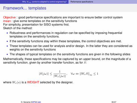
Framework... templates

Objective : good performance specifications are important to ensure better control systemmean : give some templates on the sensitivity functionsFor simplicity, presentation for SISO systems first.Sketch of the method:• Robustness and performances in regulation can be specified by imposing frequential

templates on the sensitivity functions.• If the sensitivity functions stay within these templates, the control objectives are met.• These templates can be used for analysis and/or design. In the latter they are considered as

weights on the sensitivity functions• The shapes of typical templates on the sensitivity functions are given in the following slides

Mathematically, these specifications may be captured by an upper bound, on the magnitude of asensitivity function, given by another transfer function, as for S:

|S(jω)| ≤1

|We(jω)|, ∀ω ⇔ ‖WeS‖∞ ≤ 1

where We(s) is a WEIGHT selected by the designer.



Template on the sensitivity function - Weighted sensitivity

Typical specifications in terms of S include:1 Minimum bandwidth frequency ωS2 Maximum tracking error at selected frequencies.3 System type, or the maximum steady-state tracking error ε04 Shape of S over selected frequency ranges.5 Maximum peak magnitude of S, ||S||∞ < MS .

The peak specification prevents amplification of noise at high frequencies, and also introduces amargin of robustness; typically we select MS = 2.



Template on the sensitivity function S


S(s) =1

1 +K(s)G(s)

1

We(s)=

s+ ωbε

s/MS + ωb

Generally ε ' 0 is considered, MS < 2(6dB) or (3dB - cautious) to ensuresufficient module margin.ωb influences the CL bandwidth : ωb ↑• faster rejection of the disturbance• faster CL tracking response• better robustness w.r.t. parametric

uncertainties

Template on the Sensitivity function S

Frequency (rad/sec)

Sin

gula

r V

alue

s (d

B)

10−4

10−2

100

102

104

106−60

−50

−40

−30

−20

−10

0

10Template on the sensitivity function S

MS = 2 (6dB)

ε = 1e − 3

ωb s.t. |1/We| = 0dB


Template on the function KS


KS(s) =K(s)

1 +K(s)G(s)

1

Wu(s)=

ε1s+ ωbc

s+ ωbc/Mu

Mu chosen according to LF behavior ofthe process (actuator constraints:saturations)ωbc influences the CL bandwidth : ωbc ↓• better limitation of measurement

noises• roll-off starting from ωbc to reduce

modeling errors effects

Template on the Controller*Sensitivity KS

Frequency (rad/sec)

Sin

gula

r V

alue

s (d

B)

100

105

−60

−50

−40

−30

−20

−10

0

10

M u = 2

ω bc fo r |1 / W u| = 0 d B

ε c = 1 e -3


Template on the function T


T (s) =K(s)G(s)

1 +K(s)G(s)

1

WT (s)=

εT s+ ωbt

s+ ωbt/MT

Generally εT ' 0 is considered, MSG

allows to limit the overshoot in theresponse to input disturbances.ωSG influences the bandwidth hence thetransient behavior of the disturbancerejection properties: ωbt ↓• better noise effects rejection• better filtering of HF modelling errors

10−4

10−2

100

102

104

106−60

−50

−40

−30

−20

−10

0

10Template on the Complementary sensitivity function T

Frequency (rad/sec)

Sin

gula

r V

alue

s (d

B) MT =1.5

εT =1e-3

ωbT s.t. |1/WT | = 0 dB


Template on the function SG


SG(s) =G(s)

1 +K(s)G(s)

1

WSG(s)=

s+ ωSGεSG

s/MSG + ωSG

Generally εSG ' 0 is considered,MT < 1.5 (3dB) to limit the overshoot.ωSG influences the CL bandwidth :ωSG ↑ =⇒ faster rejection of thedisturbance.

10−4

10−2

100

102

104

106−40

−30

−20

−10

0

10

20 Template on the Sensitivity*Plant SG

Frequency (rad/sec)

Sin

gula

r V

alue

s (d

B) MSG = 10

εSG=1e-2

ωsg s.t. |1/WSG| = 0 dB


A first insight into the MIMO case

The direct extension of the performances objectives to MIMO systems could be formulated asfollows:

1 Disturbance attenuation/closed-loop performances:

σ(Sy) <1

W1(jω)

with W1(jω) > 1 for ω < ωb2 Actuator constraints:

σ(KSy) <1

W2(jω)

with W2(jω) > 1 for ω > ωh3 Robustness to multiplicative uncertainties:

σ(Ty) <1

W3(jω)

with W3(jω) > 1 for ω > ωt

However these objectives do not consider the specific MIMO structure of the system, i.e. theinput-output relationship between actuators and sensors.It is then better to define the objectives accordingly with the system inputs and outputs.



Towards MIMO systems

Let us consider a system with 2 inputs and 1 output and define:

G =(G1 G2

), K =

(K1

K2

)Therefore

GK = G1K1 +G2K2, KG =

(K1G1 K1G2

K2G1 K2G2

)and the sensitivity functions are:

Sy =1

1 +G1K1 +G2K2, KSy =

(K1

1+G1K1+G2K2K2

1+G1K1+G2K2

)

While a single template We is convenient for Sy it is straightforward that the following diagonaltemplate should be used for KSy :

Wu(s) =

(W 1u(s) 00 W 2

u(s)

)where W 1

u and W 2u are chosen in order to account for each actuator specificity (constraint).



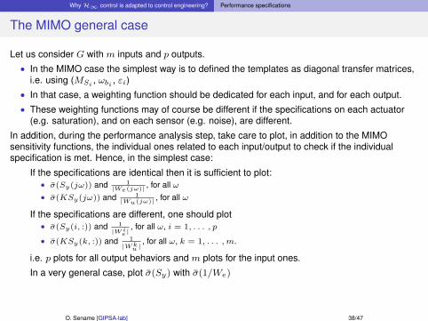
The MIMO general case

Let us consider G with m inputs and p outputs.• In the MIMO case the simplest way is to defined the templates as diagonal transfer matrices,

i.e. using (MSi, ωbi , εi)

• In that case, a weighting function should be dedicated for each input, and for each output.• These weighting functions may of course be different if the specifications on each actuator

(e.g. saturation), and on each sensor (e.g. noise), are different.

In addition, during the performance analysis step, take care to plot, in addition to the MIMOsensitivity functions, the individual ones related to each input/output to check if the individualspecification is met. Hence, in the simplest case:

1 If the specifications are identical then it is sufficient to plot:• σ(Sy(jω)) and 1

|We(jω)| , for all ω• σ(KSy(jω)) and 1

|Wu(jω)| , for all ω

2 If the specifications are different, one should plot• σ(Sy(i, :)) and 1

|Wie|

, for all ω, i = 1, . . . , p

• σ(KSy(k, :)) and 1

|Wku |

, for all ω, k = 1, . . . ,m.

i.e. p plots for all output behaviors and m plots for the input ones.3 In a very general case, plot σ(Sy) with σ(1/We)



More on weighting functions

When tighter (harder) objectives are to be met .....the templates can be defined more accurately by transfer functions of order greater than 1, as

We(s) =

(s/MS + ωb

s+ ωbε

)k,

if a roll-off of −20× k dB per decade is required.Take care to the choice of the parameters (MS , ωb, ε) to avoid incoherent objectives!

100

101

102

103

104

105

106

−80

−70

−60

−50

−40

−30

−20

−10

0

10

20

Mu=2, wbc=100, epsi1=0.01

Wu and Wu square without parameter modification

Frequency (rad/sec)

Sin

gula

r V

alue

s (d

B)

100

101

102

103

104

105

106

−50

−40

−30

−20

−10

0

10

20

Original weight (specifications) Mu=2, ε1 = 0.01, ωb c=100 for Wu

Mu =√

2, ε1 =√

0.01,ωb c=100 for 1/W 2

u case 1

Mu =√

2, ε1 =√

0.01,ωb c=200 for 1/W 2

u case 2

Mu =√

2, ε1 =√

0.01,ωb c=400 for 1/W 2

u case 3

$1/W_u$ and $1/Wu_^2$ with parameter modification

Frequency (rad/sec)

Sin

gula

r V

alue

s (d

B)



Final objectives

In terms of control synthesis, all these specifications can be tackled in the following problem: findK(s) s.t.

∥∥∥∥∥∥∥∥WeSWuKSWTT

WSGSG

∥∥∥∥∥∥∥∥∞

≤ 1 ⇒ ‖WeS‖∞ ≤ 1 ‖WSGSG‖∞ ≤ 1‖WuKS‖∞ ≤ 1 ‖WTT‖∞ ≤ 1

Often, the simpler following one (referred to as the mixed sensitivity problem) is studied:

Find K s.t.

∥∥∥∥ WeSWuKS

∥∥∥∥∞≤ 1

since the latter allows to consider the closed-loop output performance as well as the actuatorconstraints.


WhyH∞ control is adapted to control engineering? The mixed sensitivityH∞ control design


It will be shown how to formulate such a control problem using "classical" control tools. Theprocedure will be 2-steps:

• Build a control scheme s.t. the closed-loop system matrix does correspond to the tackledH∞problem (for instance the mixed sensitivity problem). Use of Matlab, sysic tool.

• Use an optimisation algorithm that finds the controller K solution of the considered problem.

Illustration on∥∥∥∥ WeSWuKS

∥∥∥∥∞≤ γ

In that case the closed-loop system must be ‖Tew(s)‖∞ =


∥∥∥∥∞≤ γ i.e a system with

1 input and 2 outputs. Since S = r−yr

and KS = ur

, the control scheme needs only one externalinput r.



How to include performance specification in H∞ control ?

Note that: in practice the performance specification concerns at least two sensitivity functions (Sand KS) in order to take into account the tracking objective as well as the actuator constraints.Control objectives:

y = Gu = GK(r − y)⇒ tracking error : ε = Sru = K(r − y) = K(r −Gu)⇒ actuator force : u = KSr

To cope with that control objectives the following control scheme is considered:

Objective w.r.t sensitivity functions: ‖WeS‖∞ ≤ 1, ‖WuKS‖∞ ≤ 1.Idea: define 2 new virtual controlled outputs:

e1 = WeSre2 = WuKSr



The mixed sensitivity H∞ control design - Problem definition

The performance specifications on the tracking error & on the actuator, given as some weights onthe controlled output, then leads to the new control scheme:

The associated general control configuration is :



The mixed sensitivity H∞ control design - Problem definition

The corresponding H∞ suboptimal control problem is therefore to find a controller K(s) such that

‖Tew(s)‖∞ =


∥∥∥∥∞≤ γ with

Tew(s) = Fl(P,K) = P11 + P12K(I − P22K)−1P21

=

[We

0

]+

[−WeGWu

]K(I +GK)−1I

=

[WeSWuKS

]in Matlab



What about disturbance attenuation ?

To account for input disturbance rejection, the control scheme must include di:

This corresponds to the closed-loop system.

Tew =

[WeSy WeSyGWuKSy WuTu

]The new H∞ control problem therefore includes the input disturbance rejection objective, thanksto SyG that should satisfy the same template as S, i.e an high-pass filter!Remarks: Note that WuTu is an additional constraint that may lead to an increase of theattenuation level γ since it is not part of the objectives. Hopefully Tu is low pass, and Wu as well.The input weight has to be on u not u+ di which would lead to an unsolvable problem.



Improve the disturbance attenuation

The previous problem, allows to ensure the input disturbance rejection, but does not provide anyadditional d-o-f to improve it (without impacting the tracking performance). In order to ’decouple’both performance objectives, the idea is to add a disturbance model that indeed changes thedisturbance rejection properties.Let then consider : di(t) = Wd.d. In that case the closed-loop system is This corresponds to theclosed-loop system.

Tew =

[WeSy WeSyGWd

WuKSy WuTuWd

]and the template expected for SyG is now 1

Wd.We.

First interest: improve the disturbance weight as Wd = 100... but this has a price (see Fig. belowfor an example)

10-2 10-1 100 101 102 103-120

-100

-80

-60

-40

-20

0

20

Mag

nitu

de (

dB)

Sensitivity*Plant SG

Frequency (rad/sec)

with Wd=1

with Wd=100

10-2 10-1 100 101 102 103-50

-40

-30

-20

-10

0

10

20

30

40

Controller*Sensitivity KS

Frequency (rad/sec)

Sin

gula

r V

alue

s (d

B)

with Wd=100

with Wd=1



More generally...

To include multiple objectives in a SINGLE H∞ control problem, there are 2 ways:1 add some external inputs (reference, noise, disturbance, uncertainties ...)2 add new controlled outputs

Of course both ways increase the dimension of the problem to be solved....thus the complexity aswell. Moreover additional constraints appear that are not part of the objectives ....General rule: first think simple !!



P. Gahinet.A linear matrix inequality approach to H∞ control.International Journal of Robust and Nonlinear Control, 4:421–448, 1994.

C. Scherer.The riccati inequality and state-space H∞-optimal control.Ph.D. dissertation, University Wurzburg, Germany, 1990.

C. Scherer, P. Gahinet, and M. Chilali.Multiobjective output-feedback control via LMI optimization.IEEE Transaction on Automatic Control, 42(7):896–911, july 1997a.

C. Scherer, P. Gahinet, and M. Chilali.Multiobjective output-feedback control via lmi optimization.IEEE Transaction on Automatic Control, 42(7):896–911, 1997b.

S. Skogestad and I. Postlethwaite.Multivariable Feedback Control. Analysis and Design.John Wiley and Sons, Chichester, 1996.

K. Zhou, J. Doyle, and K. Glover.Robust and Optimal Control.New Jersey, 1996.


robust and lpv control of mimo systems part 2: h controlo.sename/docs/hinfcontrol.pdf · robust and...

Documents