robust building detection in aerial images

ROBUST BUILDING DETECTION IN AERIAL IMAGES

Sonke Muller∗, Daniel Wilhelm Zaum

Institut fur Theoretische Nachrichtentechnik und Informationsverarbeitung, Universitat Hannover, Germany -{mueller, dzaum}@tnt.uni-hannover.de,∗corresponding author

KEY WORDS: Building, Extraction, Aerial, Segmentation, Classification, Land Use.

ABSTRACT

The robust detection of buildings in aerial images is an important part of the automated interpretation of these data. Applications aree.g. quality control and automatic updating of GIS data, automatic land use analysis, measurement of sealed areas for public authorityuses, etc. As additional data like laser scan data is expensive and often simply not available, the presented approach is based only onaerial images. It starts with a seeded region growing algorithm to segment the entire image. Then, photometric and geometric featuresare calculated for each region. Especially, robust form features increase the reliability of the approach. A numerical classification isperformed to differentiate the classes building and non-building. The approach is applied to a test site and the classification results arecompared with manually interpreted images.

1 INTRODUCTION

The detection of buildings is an important task for the interpreta-tion of remote sensing data. Possible applications for automaticbuilding detection are the creation and verification of maps andGIS data, automatic land use analysis, measurement of sealed ar-eas for public authority uses, etc.

Buildings are significant objects in remote sensing data and di-rectly indicate inhabited areas. In most cases, buildings are wellrecognizable by a human interpreter. An automatic system that isable to emulate a human operator is desired.

In the presented approach we concentrate on aerial images with aresolution of0.3125 m

pixel, because often additional costs or sim-

ple unavailability prevent the utilization of additional sensor data.

The different approaches for building detection in remote sens-ing data differ in the used type of input data. Often, multi sensorydata, e.g. SAR, infrared, stereo or laser scan images, is availableas additional information that can improve the object extraction.Some approaches, like the presented one, work only on RGB im-ages. The following section discusses some of them.

C. Lin and R. Nevatia (Lin and Nevatia, 1998) propose a buildingextraction method, that is based on the detection of edges in theimage. It is assumed that the searched rectangular buildings canbe distorted to parallelograms. The edges are taken as buildinghypothesis and classified by use of a feature vector and additionalfeatures like shadow. The found buildings are modeled as 3Dobjects.

G. Sohn and I. J. Downman (Sohn and Dowman, 2001) deal withbuilding extraction in low-resolution images. They start with aFourier transform to find dominant axes of groups of buildings,assuming that buildings are aligned parallel along a street. Dueto the low image resolution, the building contours can only befound including gaps. Theses gaps are closed using the aforedetected dominant axes. The regions found and relations betweeneach other, are stored in a tree. The tree is used to find buildingstructures.

The present approach is divided into a low-level and high-levelimage processing step. The low-level step includes image seg-mentation and postprocessing: first, the input RGB image is

transformed to HSI and the intensity channel is taken as inputfor a region growing segmentation algorithm to get a segmentedimage. The seed points of this algorithm are set flexibly underconsideration of the red channel. The segmentation result is post-processed to compensate effects like holes in the regions and tomerge roof regions which are separated into several parts. Theregions are taken as building hypotheses in the following steps.

The high-level step includes feature extraction and final classi-fication: first, a preselection is performed to reduce the numberof building hypotheses by use of the region area and color. Dur-ing the feature extraction, photometric, geometric and structuralfeatures are calculated for each hypothesis like:

• geometric features– object size: area, circumference– object form: roundness, compactness, lengthness, an-

gles, etc.• photometric features

– most frequent and mean hue• structural features

– shadow, neighborhoods

Furthermore, the main axes of building hypotheses are calculated.They define a hexagon describing the region’s contour. Eventu-ally, a numerical classification is performed to decide whether abuilding hypothesis is a building or not.

The remaining part of this paper is organized as follows: in sec-tion 2 the initial segmentation procedure is described. Section 3shows how and which features are used for the following classifi-cation step. The classification itself is described in section 4. Theexperimental results are presented in section 5 and the paper issummarized in section 6.

2 LOW-LEVEL PROCESSING

This section describes all low-level processing steps includingpreprocessing, where the input image is transformed, image seg-mentation, using a seeded region growing algorithm, and a post-processing step, that allows merging of regions that fulfill specialconditions.

In: Stilla U, Rottensteiner F, Hinz S (Eds) CMRT05. IAPRS, Vol. XXXVI, Part 3/W24 --- Vienna, Austria, August 29-30, 2005¯¯¯¯¯¯¯¯¯¯¯¯¯¯¯¯¯¯¯¯¯¯¯¯¯¯¯¯¯¯¯¯¯¯¯¯¯¯¯¯¯¯¯¯¯¯¯¯¯¯¯¯¯¯¯¯¯¯¯¯¯¯¯¯¯¯¯¯¯¯¯¯¯¯¯¯¯¯¯¯¯¯¯¯¯¯¯¯¯¯¯¯¯¯¯¯¯¯¯¯¯¯¯¯¯¯¯¯¯

143

2.1 Image preprocessing

The input images are available as raster data in RGB color space.To get a single band grey value image as input for the segmen-tation algorithm, the input RGB image is transformed to HSI. Toget the intensity channelI of the HSI transformation, the fol-lowing equation is used, where weights are set according to theperception of the human eye:

I = 0, 299 ·R + 0, 587 ·G + 0, 114 ·B (1)

The color angleH is calculated independent from the saturationand intensity and later used as a region feature:

H1 = arccos

"12((R −G) + (R −B))p

(R −G)2 + (R −B)(G−B)

#(2)

H =

(2π −H1 , if B > G

H1 , else(3)

The saturationS is calculated using equation 4:

S =max(R, G, B)− min(R, G, B)

max(R, G, B)(4)

2.2 Seeded region growing algorithm

For the initial segmentation of the input image, a seeded regiongrowing algorithm is used to find homogeneous roof regions inthe image. The seed points are regularly distributed over the im-age with a seed point raster size set with respect to the expectedroof size. For an input resolution of0.3125 m

pixel, an appropri-

ate raster size is 15 pixel to ensure that nearly every roof regionis hit. This is not possible with a standardsplit and merge al-gorithm. As input channel of the region growing algorithm, theintensity channel is taken, calculated as described before in sec-tion 2.1. Attempts to use more than one channel as input for theregion growing algorithm were made, but led to inferior results.

The seeded region growing algorithm starts at the pixel positionof each seed point and compares this pixel’s value with the neigh-boring pixel values. If the neighbor pixel values lie inside a giventolerancetT , the neighboring pixels belong to the same region asthe seed point. The region growing goes on recursively with thenewly added pixels and ends, when no new neighboring pixelswhich fulfill the condition can be found. Pixels which alreadybelong to a region are omitted. An example of an image segmen-tation made with the described procedure is shown in Fig. 2A.

To take only promising seed points, not a simple raster is takenas described up to now. The input image is divided into equallydistributed regions of the size of the seed point raster. For eachregion a histogram of the red channel is calculated. Provided thatbuilding roofs are red, brownish or grey, the red channel indicatesthe existence of roofs.

For each region, an arbitrary pixel with a red channel correspond-ing to the maximum histogram value is chosen. In order to avoidseed points in shadow regions, this value has to be larger thana thresholdtS . Fig. 1 shows the red channel of a typical partof an input image and the corresponding histogram. The regiongrowing step results in a completely segmented image.

0 25512835grey value

count n

Figure 1: Red channel of a typical part of the input image, B)Histogram with thresholdtS = 35 for selection of seed points.

2.3 Image postprocessing

The aim of the postprocessing step is to improve the image seg-mentation for the following feature extraction and classification.The postprocessing consists of two steps. The first step is openingand closing of the segmented image. The second step is mergingof special regions.

2.3.1 Opening and closing By use of opening and clos-ing operators, the ragged edges of the regions (see Fig. 2) aresmoothed and small holes in the regions are closed. As a conse-quence of the improvement of the region contours, the featuresused for classification of the regions can be calculated more pre-cisely. In Fig. 2B, the result of opening and closing operations isshown.A) B)

Figure 2: Example of the erosion and dilation step: A) imagesegmentation, B) image segmentation after applying of dilationand erosion, undersized and oversized regions are not considered.

2.3.2 Merging of regions The most important postprocess-ing step is the merging of regions belonging to the same roof. InFig. 3 two examples of roofs that have been segmented into twodifferent regions and the corresponding input images are given.Many roof regions are split at the roof ridge. Especially, com-plex roof structures like gable roofs, dormers, towers, roof-lightsand superstructures lead to multiple regions for only one building,which complicates the subsequent classification.

Figure 3: Two examples of roofs that consist of more than oneregion.

The complete merging procedure is depicted in Fig. 4. The left-most image in Fig. 4 shows a symbolic example of an input im-age, that is the basis for the next steps.

CMRT05: Object Extraction for 3D City Models, Road Databases, and Traffic Monitoring - Concepts, Algorithms, and Evaluation¯¯¯¯¯¯¯¯¯¯¯¯¯¯¯¯¯¯¯¯¯¯¯¯¯¯¯¯¯¯¯¯¯¯¯¯¯¯¯¯¯¯¯¯¯¯¯¯¯¯¯¯¯¯¯¯¯¯¯¯¯¯¯¯¯¯¯¯¯¯¯¯¯¯¯¯¯¯¯¯¯¯¯¯¯¯¯¯¯¯¯¯¯¯¯¯¯¯¯¯¯¯¯¯¯¯¯¯¯

144

region overlaps

intersection

input image

shadow image shadow lines

with shadow(after dilation)

merged

segmentationimage

regions

surroundingregions(after dilation)

Figure 4: Steps of the merging procedure.

The segmented regions are dilated two times. Assuming thatbuildings cast a shadow, roof candidates with adjoined shadowregions are determined. Therefore, a shadow detection algo-rithm, performing a simple threshold operation as described insection 3.4.2, is applied to the input image. Subsequently, onlyshadow regions with straight borders are considered. The seg-mented regions are dilated two times. Regions now significantlyoverlapping with shadow regions, i.e. the intersection area islarger than a thresholdS1, are joined with overlapping neigh-bor roof candidate regions (see Fig. 4). Again, the intersectionarea has to be larger than a second thresholdS2. Eventually, themerged roof regions are eroded two times to restore the originalregion size.

Figure 5: The result of a successful merging: labels of Fig. 3merged together.

3 FEATURE EXTRACTION

This section describes the used numeric features which are ex-tracted for each roof hypothesis. The result of the feature ex-traction, the numeric feature vector, is the basis for the followingclassification.

3.1 Preselection

To reduce calculation time, a preselection is performed, whichsorts out implausible roof hypotheses. Roof hypotheses that aresorted out are eliminated and kept unconsidered during the clas-sification. Therefore, the preselection has to be carried out care-fully to prevent the loss of correct roofs. The features used forthe preselection step are the region area and the mean hue angle.

3.1.1 Area The area of a roof hypothesis is calculated bycounting the pixels of a region including holes. A hypothesisis assumed valid if theareafulfills equation 5.

30 pixels< area < 25000 pixels (5)

3.1.2 Mean hue angle The second exclusion criterion is thecolor of a roof hypothesis. Therefore, the mean hue value of thepixels belonging to the corresponding region is calculated. Fig. 6shows an example histogram of hue values for a roof region. Themean hue angleHm is calculated as follows:

• in the range from360◦ to 540◦ the hue value histogram isextended periodically

• if more than5% of the pixels’ hue values lie between0◦ and20◦ or 340◦ and360◦ respectively:

– calculate the mean in the range from180◦ to 540◦

• else:– calculate the mean in the range from0◦ to 360◦

360°0° 540° color

count

color angle

0°

360°

unroll

count

angle

red red

Figure 6: Example histogram of hue values for one roof hypoth-esis.

As explained before, roofs of buildings are perceptible in the redchannel. All roof hypotheses with a mean hue valueHm close togreen, see equation 6, are rejected.

115 < Hm < 125 (6)

3.2 Geometric features

This section describes the geometric features used and how theyare calculated.

3.2.1 Size features The size features of a roof hypothesischosen are theareaandcircumference. The area is already cal-culated during the preselection step as described in section 3.1.1.The calculation of the circumference of a building is depicted in


145

Fig. 7: the left image shows a segmented roof candidate region,the right one shows its contour calculated with an outlining pro-cedure. The counted contour pixel are used as circumference.

Figure 7: Outlining procedure: segmented roof region and regioncontour.

3.2.2 Form features Form features are very important be-cause the form can distinguish buildings from natural objects.Buildings are normally constructed with right angles. The fea-tures used are thereforeroundness, compactness, lengthnessandcharacteristic anglesof a region.

Theroundness is calculated independently of the region’s sizeas ratio of area to the square of the circumference. It ranges from0 to 1.

roundness =4π · area

circumference2(7)

Thecompactnessof a region is defined as number of erosion stepsthat are necessary to remove the region in complete.

In (Baxes, 1994), different types of region axes are introduced.The main axis is defined as the line between two contour pointsthat have the maximum distance among each other.

The two ancillary axes are defined as vertical lines to the mainaxis with the maximum distance from the contour to the mainaxis. For each side of the main axis one ancillary axis is defined.

The cross axis is defined as vertical line to the main axis thatconnects two contour points with the maximum distance to eachother.

The axes calculation results in six points which lie on the contourof the investigated region. The corresponding hexagon approxi-mates the region’s shape. An example of such a hexagon is shownin Fig. 8.

α

main axis

cross axis

β

ancillary axes

Figure 8: Approximating hexagon model.

The anglesα andβ, as depicted in in Fig. 8, are used as additionalfeatures. In most buildings these two angles are approximately

right angles: on the left hand side of Fig. 9 a segmented buildingand its corresponding angles is illustrated. The described anglesactually are approximately right angles. On the right hand side ofFig. 9 a segmented forest region is shown. Here, the angles arenot close to being right angles.

Figure 9: Examples for roof hypothesis.

The featurelengthnessis also based on the calculated axes of aregion. It is the ratio of the main axis length to the cross axislength.

Finally, it is measured how frayed a region is. Pixels that lieinside the hexagon and do belong to the investigated region(hexagon area inside) are counted, as well as the region pixelsthat lie outside the hexagon (hexagon area outside). The ratioof hexagon area insideto hexagon area outsideis a feature thatdescribes how frayed a region is.

Rectangular buildings with smooth contours fill the hexagon incomplete, in contrast to e.g. parts of a segmented forest.

3.3 Photometric features

Two photometric features are calculated that are based on the hueangle histogram of the region pixels.

3.3.1 Hue angle After applying a threshold on the intensitychannel to discard shadow regions, the maximum value of thehue angle histogram of a region is taken as a feature.

3.3.2 Mean hue angle Additionally, the mean hue angle of abuilding hypothesis as already described in section 3.1.2 is cho-sen as a feature.

3.4 Structural features

Structural features use information about neighboring regions andshadow.

3.4.1 Neighborhoods Buildings are usually not freestand-ing but appear in groups. Consequently, buildings with otherbuildings nearby are more probable than single buildings. Foreach building hypothesis the neighboring buildings are counted.Neighbor means that the distance center to center is smaller thana thresholdTN . The number of neighboring buildings is used tosupport or reject unsteady hypothesis.

3.4.2 Shadow The acquisition of aerial images requires goodweather conditions, so the existence of shadow can be used for theextraction of buildings. Shadows are expected next to buildings,and therefore give hints to where buildings are.

The extracted shadow regions, shown in Fig. 10B, are obtainedby a threshold decision on the intensity channelI of the input im-age. Only shadow regions with straight borders are considered.The first feature derived from extracted shadow is the general ex-istence of shadow next to a building, the second is the ratio ofregion pixel that overlap with shadow, after a double dilation ofthe region.


146

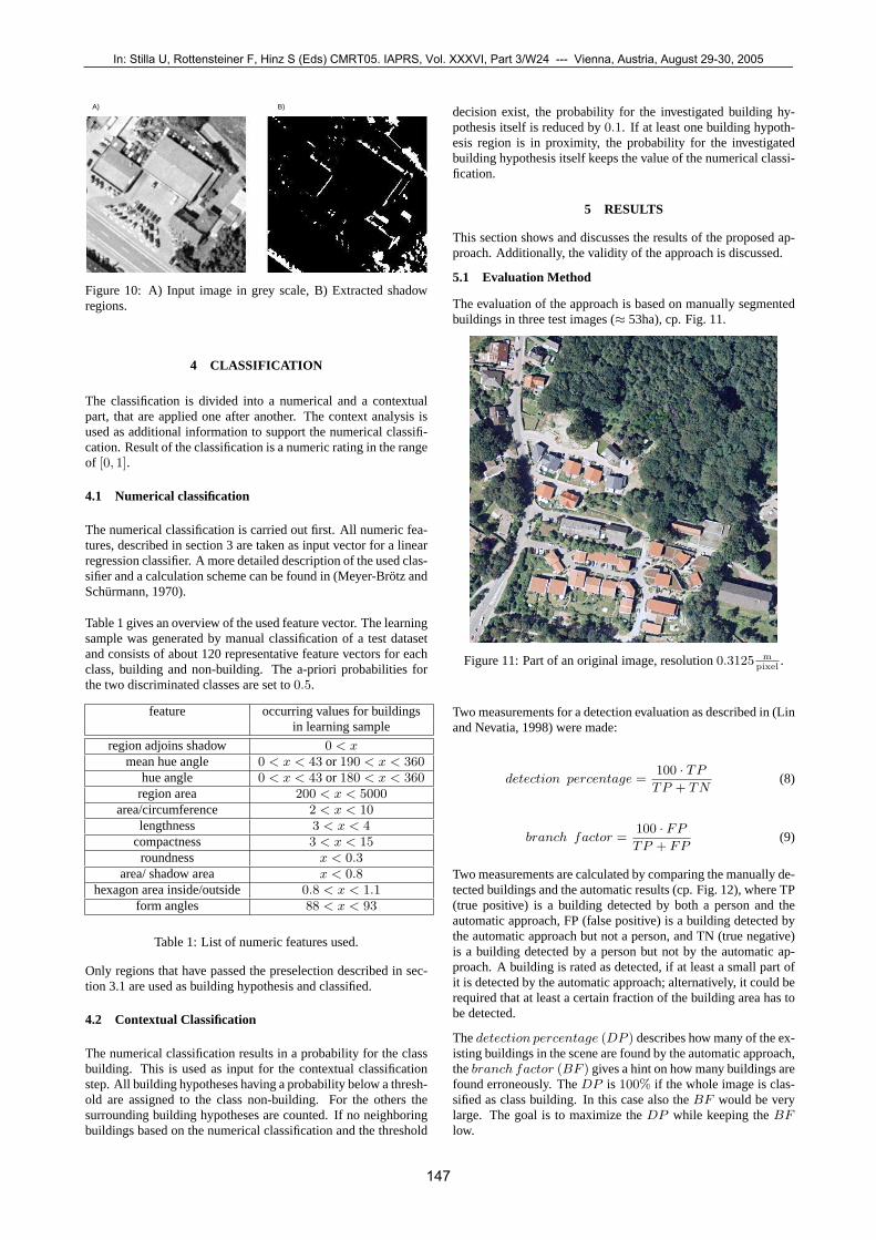
A) B)

Figure 10: A) Input image in grey scale, B) Extracted shadowregions.

4 CLASSIFICATION

The classification is divided into a numerical and a contextualpart, that are applied one after another. The context analysis isused as additional information to support the numerical classifi-cation. Result of the classification is a numeric rating in the rangeof [0, 1].

4.1 Numerical classification

The numerical classification is carried out first. All numeric fea-tures, described in section 3 are taken as input vector for a linearregression classifier. A more detailed description of the used clas-sifier and a calculation scheme can be found in (Meyer-Brotz andSchurmann, 1970).

Table 1 gives an overview of the used feature vector. The learningsample was generated by manual classification of a test datasetand consists of about 120 representative feature vectors for eachclass, building and non-building. The a-priori probabilities forthe two discriminated classes are set to0.5.

feature occurring values for buildingsin learning sample

region adjoins shadow 0 < xmean hue angle 0 < x < 43 or 190 < x < 360

hue angle 0 < x < 43 or 180 < x < 360region area 200 < x < 5000

area/circumference 2 < x < 10lengthness 3 < x < 4

compactness 3 < x < 15roundness x < 0.3

area/ shadow area x < 0.8hexagon area inside/outside 0.8 < x < 1.1

form angles 88 < x < 93

Table 1: List of numeric features used.

Only regions that have passed the preselection described in sec-tion 3.1 are used as building hypothesis and classified.

4.2 Contextual Classification

The numerical classification results in a probability for the classbuilding. This is used as input for the contextual classificationstep. All building hypotheses having a probability below a thresh-old are assigned to the class non-building. For the others thesurrounding building hypotheses are counted. If no neighboringbuildings based on the numerical classification and the threshold

decision exist, the probability for the investigated building hy-pothesis itself is reduced by0.1. If at least one building hypoth-esis region is in proximity, the probability for the investigatedbuilding hypothesis itself keeps the value of the numerical classi-fication.

5 RESULTS

This section shows and discusses the results of the proposed ap-proach. Additionally, the validity of the approach is discussed.

5.1 Evaluation Method

The evaluation of the approach is based on manually segmentedbuildings in three test images (≈ 53ha), cp. Fig. 11.

Figure 11: Part of an original image, resolution0.3125 mpixel

.

Two measurements for a detection evaluation as described in (Linand Nevatia, 1998) were made:

detection percentage =100 · TP

TP + TN(8)

branch factor =100 · FP

TP + FP(9)

Two measurements are calculated by comparing the manually de-tected buildings and the automatic results (cp. Fig. 12), where TP(true positive) is a building detected by both a person and theautomatic approach, FP (false positive) is a building detected bythe automatic approach but not a person, and TN (true negative)is a building detected by a person but not by the automatic ap-proach. A building is rated as detected, if at least a small part ofit is detected by the automatic approach; alternatively, it could berequired that at least a certain fraction of the building area has tobe detected.

Thedetection percentage (DP ) describes how many of the ex-isting buildings in the scene are found by the automatic approach,thebranch factor (BF ) gives a hint on how many buildings arefound erroneously. TheDP is 100% if the whole image is clas-sified as class building. In this case also theBF would be verylarge. The goal is to maximize theDP while keeping theBFlow.


147

Figure 12: Classification result: Building polygons marked inblue.

5.2 Evaluation results of a test dataset

The analysis is tested on a set of three images of about1500 ×1200 pixels. Each image contains about 120 buildings. The re-sults are shown in detail in Table 2 and the mean values for thewhole test site in Table 3.

image TP FP TN DP BF

W1 89 28 18 83.2% 23.9%W2 109 34 24 82.0% 23.8%W3 85 21 31 73.3% 19.8%

Table 2: Evaluation results of three test images.

mean values of images DP BF

W1, W2, W3 79.5% 22.5%

Table 3: Mean results of three test images.

5.3 Validity of the results

The classification uses a knowledge base that was optimized tothe test data set of a rural area. The approach runs satisfactorilyin regions of small towns with characteristic one family houses,small apartment houses, and industrial areas. One aspect of theclassification was to reliably detect or reject vegetation areas, thatare not dominant in downtown areas. The knowledge base isalso not optimized for detection of multistory buildings and townhouses. Due to the modular structure of the proposed approach,the knowledge base can be easily expanded to other situations.

The approach was additionally tested on a set of IKONOS im-ages with a spatial resolution of 1.0m. This test was done with-out manual parameter tuning. Due to the lack of a precise manualsegmentation, a numerical evaluation was not done, but the re-sults look comparably good to those of the tested aerial images(see Fig. 13). Oversegmentation caused by not optimally adaptedthresholds during low-level processing does not affect the detec-tion result, since it is based on robust features.

Figure 13: Classification result of an IKONS image: Buildingpolygons marked in blue.

6 CONCLUSIONS

We propose an algorithm to detect buildings in aerial images. Aseeded-region growing algorithm is used to segment the entireimage. A preselection reduces the feature extraction to only plau-sible hypothesis. The classification is based on robust features,especially form features. The numerical linear regression clas-sifier is extended by a contextual classification, considering thesurroundings of a building.

To evaluate the building detection approach, it is tested on asite of≈ 53ha. The results in Table 3 show that the proposedapproach is applicable. Other approaches sometimes achievesmallerbranch factors. However they mostly concentrate onsmall images. This leads to a smallerbranch factor. In thepresent approach, test sites including large vegetation areas areused. In consideration of today’s available computing power, rep-resentative test sites have to be tested to get expressive results.

The runtime of the present approach depends on the image con-tent. The low-level processing requires the major part of the pro-gram runtime. The algorithm’s runtime on a 2.8GHz Pentium4computer is 45 to 75 minutes for an image of 6400 x 6400 pixels.

REFERENCES

Baxes, G. A., 1994. Digital image processing: principles andapplications. John Wiley & Sons, Inc., New York, NY, USA.

Lin, C. and Nevatia, R., 1998. Building detection and descrip-tion from a single intensity image. Computer Vision and ImageUnderstanding: CVIU 72(2), pp. 101–121.

Meyer-Brotz, G. and Schurmann, J., 1970. Methoden der au-tomatischen Zeichenerkennung. K. Becker-Berke and R. Her-schel, R. Oldenbourg Verlag, Munchen-Wien.

Sohn, G. and Dowman, I. J., 2001. Extraction of buildings fromhigh resolution satellite data. In: Proc. ASCONA 2001, Ascona,Swiss, pp. 345–355.


148

robust building detection in aerial images

Documents