robust cyclic scheduling applied to container … · robust cyclic scheduling applied to container...
TRANSCRIPT

Robust cyclic scheduling applied to container
management of medium sized seaport
Hongchang Zhang
To cite this version:
Hongchang Zhang. Robust cyclic scheduling applied to container management of medium sizedseaport. Automatic. Ecole Centrale de Lille, 2014. English. <NNT : 2014ECLI0018>. <tel-01266195>
HAL Id: tel-01266195
https://tel.archives-ouvertes.fr/tel-01266195
Submitted on 2 Feb 2016
HAL is a multi-disciplinary open accessarchive for the deposit and dissemination of sci-entific research documents, whether they are pub-lished or not. The documents may come fromteaching and research institutions in France orabroad, or from public or private research centers.
L’archive ouverte pluridisciplinaire HAL, estdestinee au depot et a la diffusion de documentsscientifiques de niveau recherche, publies ou non,emanant des etablissements d’enseignement et derecherche francais ou etrangers, des laboratoirespublics ou prives.

N° d’ordre : 255
ECOLE CENTRALE DE LILLE
THESE
présentée en vue d‟obtenir le grade de
DOCTEUR
en
Spécialité: Automatique Génie Informatique, Traitement du Signal et Images
Par
Hongchang ZHANG
DOCTORAT DELIVRE PAR L’ECOLE CENTRALE DE LILLE
Titre de la thèse
Ordonnancement cyclique robuste appliqué à la gestion des
conteneurs dans les ports maritimes de taille moyenne
Robust cyclic scheduling applied to container management of
medium sized seaport
Soutenue le 10 decembre 2014 devant le jury d‟examen:
Président Pr. Gilles GONCALVES Universié d‟Artois
Rapporteur Pr. Isabel DEMONGODIN Université Aix-Marseille
Rapporteur Pr. Dimitri LEFEBVRE Université du Havre
Membre MCF, Patrice BONHOMME INSA, Centre Val de Loire
Directeur de thèse MCF, HDR Khaled MESGHOUNI Ecole Centrale de Lille
Co-directeur de thèse DR Simon COLLART-DUTILLEUL IFSTTAR, Lille
Thèse préparée dans le Laboratoire d‟Automatique, Génie Informatique et Signal
L.A.G.I.S., CNRS UMR 8219 – Ecole Centrale de Lille
Ecole Doctorale Sciences pour l‟ingénieur ED 072
PRES Université Lille Nord-de-France

À ma fille
à ma femme
à toute ma famille
à mes professeurs
et à mes chèr(e)s ami(e)s
感谢,我的女儿
妻子
家人
导师
和朋友!

i
Acknowledgements
This work would not have been done by the help and supports of the kind people
around me. I would like to take the opportunity to express the gratitude to thank all
my friends and colleagues that have given me supports and encouragement during my
thesis work.
First of all, I would like to express my deepest sense of gratitude to my supervi-
sors, Mr. Khaled MESGHOUNI and Prof. Simon COLLART-DUTILLEUL, who of-
fered their systematic guidance, meaningful advices, continuous patience and encour-
agement throughout the course of this thesis.
I acknowledge my very sincere gratitude to the jury members of my PHD com-
mittee. Thanks Prof. Isabel DEMONGODIN and Prof. Dimitri LEFEBVRE, who
have reviewed carefully my thesis. And I also express my very heartfelt thanks to
Prof.Gilles GONCALVES amd Mr. Patrice BONHOMME, for their helpful advices
and sharing of researching experience.
I would like to thanks the members in the research team “Optimisation des Sys-
tème Logistiques (OSL)”. With their help, I have learnt a lot in the relative research
domains and directions.
This research is also partially supported by the project PERFECT of the ANR.
We sincerely thank the kindly assistance.
I am also thankful to all my colleagues in my office, Baisi LIU, Rahama
LAHYANI, Lijuan ZHANG, Ben Li. Thanks to them, I have an agreeable and peace-
ful research environment. My thanks also go to Vanessa Fleury, Christine Yvoz and
Brigitte Foncez , they help me a lot in the administrational work. I also want to thanks
Jacques and Patrick for their technician support in so many times.
My sincere appreciations also go to my friends, Daji, Zhanjun, Yu, Chen, Lijie,
Youwei, Qi, Jing, Wan, Yihan, Bing,..., for their friendship and a lot of help, which
bring so much convenience and happiness to my three years life in Lille. And I also
thanks to all my French friends, they make me know a lot about the excellent French
culture and the interesting history. I love France, and I love the kind and generous
people in this country.
Finally, I take this opportunity to express the profound gratitude from the deep
bottom of my heart to my beloved daughter Huanyan, my wife Yan, my parents, my
brother, and all my families for their love and continuous emotional support that
makes me be able to overcome the difficulties in the research life. In this three years,

ii
their encouragement and support make me clam and peaceful when I miss so much
the life with them in China.

iii
Table of Contents
Acknowledgements .................................................................... i
Table of Contents .................................................................... iii
List of Tables ............................................................................ ix
List of Figure ............................................................................ xi
Abbreviations ........................................................................ xiii
General Introduction ................................................................ 1
Motivation ........................................................................................................ 1
About InTraDE.............................................................................................. 1
Our work boundary ....................................................................................... 2
The reason to use cyclic scheduling for robust control ................................ 3
The methods and tools used in this thesis ..................................................... 4
Contributions .................................................................................................. 5
Outline of the thesis ........................................................................................ 6
Chapter 1 Literature Review .................................................. 9
1.1 Seaport container terminal and non-cyclic container transit ....... 10
1.1.1 About container terminals............................................................... 11
1.1.1.1 Present situation and trends ...................................................... 11
1.1.1.2 Equipment and workflow ......................................................... 13
1.1.2 Non-cyclic vehicles scheduling in container terminals .................. 15
1.2 Cyclic job-shop problem (CJSP) by using Petri Net ..................... 17
1.2.1 Petri nets for handling time problem .............................................. 18
1.2.2 P-time strongly connected event graph (PTSCEG) ........................ 20
1.3 Cyclic job-shop problem (CJSP) based on MIP............................. 22
1.3.1 The main structure of MIP model ................................................... 25
1.3.1.1 The structure of MIP model for minimizing the cycle time ..... 26

iv
1.3.1.2 The structure of MIP model for minimizing the WIP .............. 26
1.3.2 Cutting techniques for MIP models ................................................ 27
1.4 Robust control of cyclic scheduling ................................................. 28
1.4.1 Strategy analysis of robust control ................................................. 29
1.4.2 Robust scheduling techniques ......................................................... 29
1.4.2.1 Non-cyclic robust scheduling ................................................... 29
1.4.2.2 Cyclic robust scheduling .......................................................... 30
1.5 Conclusion ......................................................................................... 34
Chapter 2 P-time Strongly Connected Event Graph
(PTSCEG) Modeling Techniques .................................................. 35
2.1 PTSCEG definition and a job-shop example ................................. 36
2.1.1 Definitions about PTSCEG ............................................................. 36
2.1.2 PTSCEG job-shop model ................................................................ 37
2.2 The container transit procedures in seaport .................................. 39
2.3 Problem definition of the container transit procedures ................ 41
2.4 PTSCEG model techniques for container transit procesures ....... 44
2.4.1 Routes modelling ............................................................................. 45
2.4.2 Place capacity modelling ................................................................ 45
2.4.3 Shared crane operation space modelling ....................................... 46
2.4.4 Intersections modelling ................................................................... 47
2.4.5 Ratio-driven task modelling ............................................................ 49
2.4.5.1 The Hillion-like modelling technique ...................................... 49
2.4.5.2 The OHL-like modelling technique ......................................... 51
2.4.6 The complete container transit PTSCEG model ............................. 52
2.5 Cutting techniques ............................................................................ 55
2.5.1 The bound of the cycle time ............................................................ 55
2.5.2 The bound of tokens with demanded cycle time .............................. 56
2.6 Conclusion ......................................................................................... 57

v
Chapter 3 Mixed Integer Programming (MIP) modeling
techniques for cyclic scheduling .................................................... 59
3.1 The constraint family explanation ................................................... 60
3.1.1 Constraints on all the places........................................................... 61
3.1.2 Constraints on places in the process circuits ................................. 64
3.1.3 Constraints on places in the space status circuits .......................... 65
3.1.3.1 Constraint families in the non-shared space status circuits ...... 66
3.1.3.2 Constraint families in the shared space status circuits ............. 67
3.2 The complete MIP models ................................................................ 69
3.2.1 The MIP model for minimizing the cycle time ................................ 70
3.2.1.1 Lower bound of cycle time ....................................................... 71
3.2.1.2 The constraint number analysis ................................................ 72
3.2.2 The MIP model for minimizing the token number .......................... 72
3.2.2.1 Lower bound of token number ................................................. 73
3.2.2.2 The constraint number analysis ................................................ 73
3.3 Case study of the seaport container transit .................................... 74
3.1 Analysis of computing time .............................................................. 79
3.2 The comparison with other similar models .................................... 80
3.3 Conclusion ......................................................................................... 82
Chapter 4 Robust Control for the 1-cyclic Scheduling ...... 83
4.1 The algorithms based on the control of transitions ....................... 84
4.1.1 Basic notation ................................................................................. 84
4.1.2 Approach 1: Rejection of the disturbance on propagation path ..... 88
4.1.2.1 Algorithm ................................................................................. 88
4.1.2.2 Description of the algorithm .................................................... 89
4.1.2.3 Analysis of the algorithm ......................................................... 90
4.1.2.4 Illustrative example .................................................................. 90

vi
4.1.3 Approach 2: Rejection of the disturbance and generation of the
parallel disturbance ............................................................................................ 94
4.1.3.1 Algorithm ................................................................................. 98
4.1.3.2 Description of the algorithm .................................................... 99
4.1.3.3 Analysis of the algorithm ....................................................... 100
4.1.3.4 Illustrative example ................................................................ 100
4.1.4 Comparison between Approach 1 and Approach 2 ...................... 103
4.2 The algorithm based on direct control of tokens’ sojourn time . 105
4.2.1 Basic notation ............................................................................... 106
4.2.1.1 The transmissible margin of the parallel similar temporal shift
group 109
4.2.1.2 The compensable margin of the disturbance rejection group 112
4.2.2 Approach 3: Generation of the parallel similar disturbance as soon
as the disturbed is observed .............................................................................. 118
4.2.2.1 Algorithm ............................................................................... 119
4.2.2.2 Description of the algorithm .................................................. 121
4.2.2.3 Analysis of the algorithm ....................................................... 121
4.2.2.4 Illustrative example ................................................................ 123
4.2.3 Comparisons with Approach 1 and Approach 2 ........................... 126
4.3 Conclusion ....................................................................................... 129
Chapter 5 Conclusions and Perspectives ........................... 131
Conclusions .................................................................................................. 131
Perspectives ................................................................................................. 133
Appendices ............................................................................ 135
Glossary ................................................................................. 137
Résumé étendu en Français ................................................. 141
Introduction ................................................................................................. 141
Chapitre 1 Etat de l’art .............................................................................. 143
vii
Chapitre 2 Graphe d’évènement P-temporels fortement connexes
(PTSCEG): Techniques de modélisation .......................................................... 144
Chapitre 3 Programmation mixte en nombres entiers (MIP): Techniques
de modélisation .................................................................................................... 145
Chapitre 4 Commande robuste pour l'ordonnancement 1-cyclique ...... 146
Chapitre 5 Conclusions & Perspectives .................................................... 147
Bibliography .......................................................................... 151

viii

ix
List of Tables
Table 2.1. Production lines sequences ................................................................ 37
Table 2.2. The time windows for each place ...................................................... 38
Table 3.1. Time windows of places in process circuits ...................................... 74
Table 3.2. Computing time of MIP model .......................................................... 79
Table 4.1. Local active robustness associated to mono-synchronized paths ...... 91
Table 4.2. The similar disturbance on parallel concentrated paths ................... 101
Table 4.3: The robustness margins of 3 approaches ......................................... 128

x

xi
List of Figure
Figure 1.1: Overview of port logistics. (Roh et al., 2007) .................................. 10
Figure 1.2: Layout of the Container Terminal YANGSHAN, Shanghai, China.
http://www.dianping.com/photos/7635647................................................. 12
Figure 1.3: Different types of handling equipment. (Grunow et al., 2006) ........ 13
Figure 1.4: Flow of transports in a seaport container terminal. (Steenken et al.,
2004) ........................................................................................................... 14
Figure 1.5: Transportation and handling chain of a container.(Steenken et al.,
2004) ........................................................................................................... 15
Figure 2.1: Example of job-shop described by PTSCEG. .................................. 38
Figure 2.2: Overview of container transit in a seaport container terminal. ........ 40
Figure 2.3: The sketch structure of the container transit. ................................... 42
Figure 2.4: The route between C1 and S1........................................................... 45
Figure 2.5: Place capacity modeling by PTSCEG. ............................................. 46
Figure 2.6: The shared crane space S1 with two routes modeled by PTSCEG. . 47
Figure 2.7:The intersection X1 modeled by PTSCEG. ...................................... 48
Figure 2.8: A Hillion-like method to model ratio-driven task ............................ 50
Figure 2.9: An OHL-like method to model the ratio-driven task. ...................... 51
Figure 2.10: The complete PTSCEG model of the import container transit
procedures. .................................................................................................. 53
Figure 3.1: A PTSCEG with time windows........................................................ 62
Figure 3.2: The Gantt chart for 1-cyclic schedule in 2G . .................................. 63
Figure 3.3: The arriving time of tokens in the places. ........................................ 64
Figure 3.4: Boolean variable ij determines the tokens number. ....................... 65
Figure 3.5: 1-cyclic schedule of the token in non-shared space status circuits. . 66
Figure 3.6: 1-cyclic schedule in the shared space status circuit of S1. ............... 67
Figure 3.7: The shared space status circuit of C5 ............................................... 67
Figure 3.8: 1-cyclic schedule of the token in the shared space circuit of C5. .... 68

xii
Figure 3.9: The optimization strategy of MIP models. ....................................... 75
Figure 3.10: The stay time of AIVs in the QCs operation space. ....................... 77
Figure 3.11: The stay time of AIVs in the AYCs operation space. .................... 77
Figure 3.12: The stay time of AIVs in the paths and the intersections. .............. 78
Figure 4.1: Case of local active robustness on a synchronized transition. ......... 85
Figure 4.2: Case of local active robust margin of mono-synchronized path. ..... 87
Figure 4.3: PTSCEG model of two routes with one shared AYC. ..................... 91
Figure 4.4: One PTSCEG including concentrated paths. ................................... 95
Figure 4.5: Parallel concentrated path and disturbance propagation path. ......... 97
Figure 4.6: Generation of similar disturbance on parallel concentrated paths. 101
Figure 4.7: The signal points on the AIV running routes. ................................ 104
Figure 4.8: The coupling of the tokens presented by Gantt graph. ................... 106
Figure 4.9: The cutting of the tokens at coupling point. ................................... 107
Figure 4.10: The classification of the tokens. ................................................... 108
Figure 4.11: The transmissible margin and compensable margin for token groups.
................................................................................................................... 123
Figure 4.12: 1-cyclic schedule of example in Figure 3.1. ................................. 127
Figure 5.1: The structure and procedures of robust cyclic methodology. ........ 131

xiii
Abbreviations
AGV - Automated guided vehicle
AIV – Automated Intelligent Vehicle
ALV - Automated lifting vehicle
AYC – Automated Yard Crane
CP - Constraint Programming
InTraDE - Intelligent Transportation in Dynamic Environment
MIP - Mixed Integer Programming
MTS - Multi-trailer systems
NWE - North west Europe
PTSCEG - P-time strongly connected event graph
QC - Quay Crane
RMG - Rail-mounted gantry
RTG - Rubber-tired gantry
VRP - Vehicle routing problem
VRPST - Vehicle routing and scheduling problem with time window constraints
WIP - Work-in-progress

xiv

Introduction
1
General Introduction
This work mainly contributes to apply the robust cyclic scheduling methodology
on container transit systems using automated intelligent vehicle (AIV) in a medium
sized seaport. Our work is based on a real industrial project, the InTraDE „Intelligent
Transportation in Dynamic Environment‟. We aim to offer some references to re-
searchers and decision makers who want to implant the robust control and manage-
ment in container transit activities, or even to other industrial domains.
Motivation
About InTraDE
The InTraDE project contributes to improve internal traffic management and op-
timization of space by developing a clean, safe, intelligent transportation system for a
few ports within North West Europe (NWE).
The world seaborne trade has been developing considerably in the last decade,
mainly due to globalization and continued development of emerging countries. This
world growth has an influence on the development of ports and maritime terminals.
But within NEW, few ports are able to keep pace with this growth. Increased interna-
tional trade, with the stagnation of spaces available in these ports, leads to critical sit-
uations in terms of management of space and time. There is an urgent need to review
the entire organization of these ports. The InTraDE aims to :
• improve the productivity of small and medium sized regional ports in NWE
so they can be more competitive.
• contribute to the effort of national and European governments to divert some
traffic from road to sea by improving the efficiency of short sea shipping.
• improve operational safety and reduce environmental impact on the region.
The research directions of InTraDE are defined as follows:
• To study traffic flow within confined spaces of container terminals and de-
velop an insight into the factors influencing the overall productivity of such

Introduction
2
facilities, and to investigate existing traffic control methods and develop
new methods where necessary to improve efficiency whilst ensuring safety.
• To identify automatic navigation methods and develop new algorithms for
robust supervision, and to investigate practical issues in implementing au-
tomatic navigation system in container terminals.
• To develop an automatic traffic time-domain simulator for autonomous and
human driven-vehicles within the terminals and to carry out a design case
study of terminal layout using the simulator.
• To design, test and validate intelligent transport vehicle prototypes with dy-
namic environments inside confined spaces or combined urban-confined
spaces.
Our work boundary
Our research involved specifically, in this project InTraDE, the management and
conduct of Automated Intelligent Vehicles (AIVs) and time management for contain-
er transit procedures in a medium sized port, such as the seaport of Le Havre in
France. The objective of our work is to develop and implement a robust cyclic sched-
uling methodology for supervision and conduct of container transit systems in con-
fined spaces in the seaport. It is well known that, in the container terminals, the dis-
turbance of time delay (on the cranes or the vehicles), time advance and equipment
breakdown do exist, and can‟t be predicted or prevented. Our research strategy is to
eliminate the disturbance by an active robust control technique with a cyclic dispatch-
ing of AIVs. If the disturbance is located in the robustness margin, by the active ro-
bust control, the disturbance can be eliminated by the system itself to avoid the possi-
ble conflicts of AIVs in the confined space without changing the initial cyclic sched-
ule. If the disturbance is out of the robustness margin, the rescheduling should be
made. The robust cyclic scheduling method can reduce the rescheduling cost and
make the transit system more resilient and ensure more safety in the container transit
field.
It is assumed the AIVs can locate their own position with some signal points set
on the field. The AIVs and the cranes can keep a real time communication with a re-
mote control center which can get the exact position of each AIV and can give a con-
trol signal to any AIVs or cranes if a disturbance is observed. By using the location
sensor and the computer on the vehicle, the AIV can avoid the collisions automatical-

Introduction
3
ly between each other or with the other equipment or container stacks. And the AIV
can control their speed and waiting time to respect the scheduled staying time in a re-
source, such as the crane operation space or one route. The information communica-
tion system for the control of transit activities are shown in the following figure.
Figure 1: The information communication system in container terminals.
The reason to use cyclic scheduling for robust control
The cyclic scheduling is an attractive theme both in industrial and academic in-
ternationally. Its definition is that some set of activities can be repeated for an infinite
number of times. Such types of scheduling problems arise in various application areas,
such as compiler design, manufacturing, digital signal processing, railway scheduling,
timetabling, etc. Compared to non-cyclic scheduling, cyclic scheduling has two main
advantages. Firstly, the entire production plan can be predicted with only information
of a partial schedule in just a repetitive period. Secondly, it is easier to apply a con-
trol strategy on the regular repetitive activities, compare with the stochastic activities.
Considering the regular activities of the operations in the cyclic schedule, it is in-
deed less complex to set up a robustness algorithm for the cyclic scheduling than the
non-cyclic scheduling. It is admitted that the cyclic scheduling does not guarantee a
better productivity than the non-cyclic scheduling in an idealized environment with-
out disturbances. But, the cyclic scheduling can adapt well with the robustness algo-

Introduction
4
rithms studied in this thesis. Since the unpredictable disturbances are inevitable, the
cyclic scheduling might be a better choice from the global view point for the overall
productivity. The others scheduling methods may waste much time on dealing with
the disturbances.
The methods and tools used in this thesis
In this thesis, we use four main methods or tools to build our robust control cy-
clic scheduling methodology.
• The first mathematical tool is the P-time strongly connected event graph
(PTSCEG). The PTSCEG is a special kind of strongly connected event
graph with time windows dedicated to each place. As discussed in above
section, the confined space and time management should be studied in our
work. The places in PTSCEG can be used to model the operation space and
the routes, the time window can be used to model the staying time of AIVs
between the signal points or in the equipment operation space. And the tran-
sition of PTSCEG can be used to model the signal points which can help
control the running of AIVs. In addition, the PTSCEG can be used as a
structure base of the first and the second robustness algorithms presented in
Chapter 4 .
• The second mathematical tool is the Mixed Integer Programming (MIP).
The PTSCEG gives us an abstract model of the resources in the container
transit field with time windows. The MIP is used to compute the cyclic
schedule of the container transit system. In this schedule, the expected so-
journ time of AIVs in each resource can be given, while respecting the de-
manded or optimal productivity. The achieved sojourn time should be locat-
ed in the time windows. The PTSCEG is also a structure base for MIP in
this thesis.
• The cyclic schedule achieved by MIP can be presented as the Gantt graph.
Using Gantt graph, the schedule of AIVs and other equipment can be clearly
shown. And the Gantt graph is a structure base for the third robustness algo-
rithm in Chapter 4 .
• The robustness algorithms are used to compute the robustness margin on the
nodes of the system. All the three algorithms introduced in Chapter 4 have a

Introduction
5
computing time in polynomial complexity. The size of the studied example
in this thesis is a medium sized seaport as the port of Le Havre, which im-
plies the computing time of algorithms can be acceptable for the real indus-
trial activities.
Contributions
From the literature review in Chapter 1 , it is found that there are many research-
es on cyclic scheduling problems, the job-shop robust control problems or the vehi-
cles scheduling problems, but our work is the first to combine the cyclic scheduling
and robust control for container transportation by AIVs in the seaport.
Firstly, we want to demonstrate that the PTSCEG can be applied to model the
container transit process with a cyclic scheduling mode. The details of the modelling
techniques are well presented to model the main production elements, such as the
routes for translating the containers, the shared cranes of different routes, the intersec-
tions on the routes, the ratio-driven task, etc. It is admitted that the PTSCEG has been
applied for modelling job-shop problems in many research, but our research aims at
extending the application of PTSCEG to a special section of the supply-chain: con-
tainer transportation in the seaports. The main assumption is that, if the cyclic sched-
uling is robust, it is able to face the system variations.
Secondly, we propose two new MIP mathematical models suitable to the cyclic
scheduling of container transit system which can be modelled as PTSCEG. In our
models, the constraint families are more concise, but strong enough. The new models
do not just consider the operation constraints with time windows on the equipment
resources or the route resources, but also consider the capacity of the resources (usu-
ally the space capacity). The new MIP models are more similar to a real industrial
production system than the research results presented in the literature review, and the
new ones have a good performance in computing time. With the MIP models, we can
find the optimal cyclic schedule of AIVs for a medium sized seaport in short time.
Thus, the traffic flow within the confined spaces and the overall productivity is opti-
mized. Actually, the preliminary propositions built on a literature review have to be
validated with regard to the computing time.
Thirdly, with some modification of robust control methods shown in the litera-
ture review, we apply two robust control algorithms on the cyclic scheduling of AIVs ,

Introduction
6
using PTSCEG model as a structure base. To our knowledge, this is the first applica-
tion of robust control cyclic scheduling on vehicles in seaport terminal. Moreover, the
complexity of the computing time of these algorithms is polynomial.
Fourthly, we propose a new robust control algorithm based on the cyclic sched-
ule obtained from the MIP model. Using Gantt graph, the structure of this algorithm
is different from the two modified algorithms mentioned in the above paragraph. In a
container terminal, the modified algorithms give control on the signal points to
change the arriving time of the AIV within time windows in resources, but the new
algorithm can directly give the control on vehicles. And the new one can better pre-
sent the influence of disturbance to each AIV in the system, which maybe more inter-
esting to the manager of container transit task.
Outline of the thesis
The content of the thesis is composed of five chapters, which is basically orga-
nized in a logical order as follows.
Chapter 1 is the first phase of work which includes an extensive literature review
to acquire necessary knowledge based on the state of the art of the various tools con-
sidered. Firstly, we introduce the general container terminal structure and some non-
cyclic vehicles dispatching methods in seaports. Then, we survey the state of the art
of cyclic scheduling for job-shop problems by using Petri Net. Thirdly, the state of
the art of Mixed Integer Programming (MIP) for job-shop cyclic scheduling is pre-
sented. Finally, we focus on the research results which combine the robust control
and cyclic scheduling.
Chapter 2 concentrates on modelling the system by the P-time strongly connect-
ed event graph (PTSCEG). Firstly, some basic knowledge of P-time Petri Net is in-
troduced by using a job-shop example. Then some more complex technique are pre-
sented for modelling the shared resource in the system, the capacity of resource, the
ratio-driven products, etc. With explanations of the modelling techniques step by step,
a complete PTSCEG model is given, which describes the container transportation task
in a medium sized container terminal. Finally, the bounds of cycle time and token
numbers for a PTSCEG are discussed, which can be used as cutting techniques for
MIP model in Chapter 3.

Introduction
7
Chapter 3 focuses on the MIP mathematical modelling of the system which can
be modelled as the PTSCEG. The modelling technique is explained step by step using
a simple example. This MIP method is applied on the container transit model
PTSCEG model presented in Chapter 2 . The MIP model here is used to give a cyclic
schedule and compute the expected sojourn time of tokens within the time windows.
The objective is to minimize the cycle time of the system and to minimize the number
of AIVs. A comparison between our method and the previous methods is made,
which shows our MIP models can better model the container transit procedures and
have a good performance in computational time.
Chapter 4 highlights the combination of robust control and cyclic scheduling.
Three algorithms are introduced. The first and the second are based on the structural
control of transitions in a PTSCEG, which can give a robustness margin on the ob-
servable and controllable nodes of the system. If the disturbance is located in the ro-
bustness margin, the system can recover to initial cyclic mode by changing the firing
time of the transitions without rebuilding the structure of the system. The third algo-
rithm plays the same role in giving the robustness margin, which is based on the anal-
ysis of the cyclic schedule shown by Gantt graph. This algorithm gives the direct ro-
bust control on the sojourn time of each token in the places. The comparison among
these three algorithms is made on the computing time complexity and the range of the
robustness margin.
Chapter 5 concludes the contributions and the originalities of this thesis. Some
interesting perspectives for further work are also proposed.

Introduction
8

Literature Review
9
Chapter 1 Literature Review
There are few literatures concerning about the robust cyclic scheduling method-
ology for the container transportation by automated intelligent vehicles (AIV) in the
seaport. Hence, the literature review of this thesis has to be based on a widespread
article study and a sophisticated collection of necessary methods or tools from a lot
of related documents of different research domains, such as the seaport organization
and container transit procedures, the Petri Nets which might be used to model the
container transit procedure, the confined space and time domains, the mixed integer
programming method which can be used to optimize the AIV flow to realize a maxi-
mal productivity, and the robust algorithms which can give a robust supervision and
management on the automated stevedoring and container transit system.
In many literatures, the mathematical tools used in this thesis are often applied
on the cyclic job-shop problems. Some kinds of these job-shop problems are very sim-
ilar to the container transit procedures in the container terminal. The products can be
seen as the containers, the transfers can be seen as the AIVs, the shared machines of
different products can be seen as the shared cranes or intersections, etc. These simi-
larities imply the possible transferability of the application of the mentioned methods
form job-shop problem to our automated container transit system. Basing on the
study of these methods, we finally extend their utilities to the sub section of the mari-
time supply chain: the container transportation in container terminals.
This chapter is organized as the follows.
Firstly, the general structure of container terminals and some non-cyclic con-
tainer transit methods are introduced. Then, the state of the art of Petri Net for mod-
elling job-shop cyclic scheduling is surveyed. Thirdly, the Mixed Integer Program-
ming (MIP) for cyclic job-shop scheduling is presented. Finally, we focus on the re-
search results combining the robust control and the cyclic scheduling.
.

Literature Review
10
1.1 Seaport container terminal and non-cyclic container transit
Firstly, the basic introduction of container terminals and the non-cyclic container
transit scheduling are presented. The study of the container terminals includes the
survey on the composition, function and complexity of the container terminals. This
research makes the PTSCEG model or MIP model more consist with the reality, and
can make us better understand the necessity to apply robust control in the container
transit procedures. The study of the non-cyclic scheduling can give us some ideas
about which are the most important criteria usually used to evaluate the container
transit performance. These criteria can be used in the optimization of our cyclic con-
tainer transit schedules. However, there are few cyclic container transit literatures can
be referred.
Figure 1.1: Overview of port logistics. (Roh et al., 2007)

Literature Review
11
1.1.1 About container terminals
1.1.1.1 Present situation and trends
In the last ten years, the ocean shipping has developed enormously. With in-
creasing logistics demands of international commercial activities, a more efficient and
more robust ocean transportation system is sought for reducing the supply-chain cost
and for assuring the safety and the stability of the system (Zaghdoud et al., 2012).
In the maritime transportation, the use of containers for intercontinental mari-
time transport has dramatically increased. A further continuous increase is expected
in the upcoming years. With an improved hull design, the modern cargo ships guaran-
tee lower transportation cost and lower CO2 emission than before, but they also give
new challenges to seaport container terminals which should be more efficient, clean
and robust. In 2013, the biggest container ship in the world Mærsk Mc-Kinney
Møller was launched. It can take 18,270 TEU (twenty-foot equivalent unit containers).
With a large number of containers for the stevedoring request, it is possible to find
some cyclic process in the container unloading/uploading or transit work among the
cranes and the container stacks. The cyclic scheduling may be one choice of the
scheduling methods to be applied in this kind of industrial procedures.
At the same time, the seaport competition is becoming ever more complex. The
maritime terminal is no longer seen just as a simple place for cargo handling, but a
functional element in a dynamic logistics chain, through which commodities, people,
and information flow (Van de Voorde and Winkelmans, 2002). Figure 1.1 illustrates a
typical port logistics process in port: from ocean shipping to inland destination for
import cargo. In this thesis, only the stevedoring and the transit of containers by AIVs
in container terminals are studied, as shown in the red rimmed boundary in Figure 1.1.
It is admitted that the seaport is a complex system including the berthing of the vessel,
the stevedoring (unloading or uploading) of containers, the transit of containers, the
stacking of containers, the cargo trucking, cargo warehouses, ship repairing, port in-
formation services , ship suppliers, the use of bunkering service before starting anoth-
er voyage etc. (Roh et al., 2007). In the various handling, transportation and storage
activities, the managers have only incomplete knowledge about future events, such as
the changing arrival time of vessels, the location of containers in the vessel or in the
yard, and even the weather condition. These information changes often, which needs
a quick reactive scheduling. Moreover, the disturbances of the time delay or advance
due to the cranes or the vehicles occur inevitably from time to time. The robust con-

Literature Review
12
trol of the container terminal system is urgently sought to eliminate the disturbances,
especially in the medium sized seaports with only the confined operation space.
Over the recent years, there is also an ongoing trend in the development of sea-
port container terminal configurations to use automated container handling and trans-
portation technology, particularly, in countries with high human resource cost. The
manually driven cranes are going to be replaced by automated ones, and the automat-
ed guided vehicles (AGVs) are used instead of manually driven carts. Figure 1.2 illus-
trates the layout of one of the most highly automated seaport container terminal in
China. This YANGSHAN port in Shanghai has a container handling capacity of 15
million TEU per year. These biggest modern seaports have very big operation filed.
But, for the medium sized ports within NWE, it is not practical to expand the terminal
filed scale in short time, considering the huge investment and the possible influence
to the nature environment. Factually, for increasing handling capacities of the medi-
um sized container terminals, the significant gains in productivity should be achieved
through advanced terminal layouts, more efficient IT-support and improved logistics
control software systems, as well as automated transportation and handling equipment.
That‟s the motivation why the InTraDE project is proposed, especially why the AIV
is designed.
Figure 1.2: Layout of the Container Terminal YANGSHAN, Shanghai, China.
http://www.dianping.com/photos/7635647

Literature Review
13
1.1.1.2 Equipment and workflow
The seaport container terminals not just greatly differ in size, but also in the type
of transportation and handling equipment used. Regarding quay cranes (QC), single
or dual-trolley cranes can be found. The latter employs an intermediate platform for
buffering the loaded and unloaded container. It is supposed that, in our work, the
quay crane can only take one container at a time. The most common types of yard
cranes are rail-mounted gantry (RMG) cranes, rubber-tired gantry (RTG) cranes,
straddle carriers, reach stackers and chassis-based transporters. Of these types of
cranes only RMG cranes are suited for fully automated container handling which will
be used as the automated yard cranes (AYC) in this thesis. Figure 1.3 exhibits the
working principle of the different types of handling equipment and their comparative
performance figures with respect to the number of TEUs, which can be stored per
hectare. Different types of vehicles can be used both for the ship-to-yard transporta-
tion and the interface between the yard and the hinterland. The most common types
are multi-trailer systems (MTS) with manned trucks, automated guided vehicles
(AGVs), and automated lifting vehicles (ALVs). The latter ones, in contrast to AGVs,
are capable of lifting a container by themselves (Yang et al., 2004). In the InTraDE
project, the definition of Automated Intelligent Vehicle (AIV) is proposed. The char-
acteristics of the AIV are inspired from those of AGV (Zaghdoud et al., 2012), but the
AIV can move autonomously and intelligently not just by the command of control
center. The AIV is not still applied in the real container transportation task. But some
tests for AIVs in the real container terminals have been done.
Figure 1.3: Different types of handling equipment. (Grunow et al., 2006)

Literature Review
14
Although the container terminals considerably differ in size, function and geo-
metrical layout, they principally consist of the same sub-systems, as shown in Figure
1.4. The ship operation or berthing area is equipped with quay cranes for the loading
and unloading of vessels. Import as well as export containers are reserved for reefer
containers, which need electrical supply for cooling, or to store hazardous goods.
Separate areas are used for empty containers. Some terminals employ sheds for stuff-
ing and stripping containers or for additional logistics services. The truck and train
operation area links the terminal to outside transportation systems (Steenken et al.,
2004).
Figure 1.4: Flow of transports in a seaport container terminal. (Steenken et al.,
2004)
The Figure 1.5 shows chain of operations for export (or import) containers. After
arrival at the terminal by truck or train, the container is identified and registered with
its major data (e.g. content, destination, outbound vessel, shipping line), picked up by
internal transportation equipment and distributed to one of the storage blocks in the
yard. The respective storage location is given by row, bay, and tier within the block in
and is assigned in real time upon arrival of the container in the terminal. To store a
container at the yard block, specific cranes or lifting vehicles are used. Finally, after
arrival of the designated vessel, the container is unload from the yard block and
transported to the berth where quay cranes load the container onto the vessel at a pre-
defined stacking position. The operations necessary to handle an import container are
performed in the reverse order (Jeon et al., 2011).
Totally speaking, it is a very complex task to schedule the huge number of con-
current operations with all the transportation and handling equipment involved. In
view of the ever changing terminal conditions and the limited predictability of future
events and their timing, this control task has to be solved in real time (Grunow et al.,

Literature Review
15
2006), and should be robust. In our work, with limited number of cranes and contain-
er stacks, the MIP can give a cyclic schedule in a short time for the container transit
procedures. And the robustness algorithms can give the robustness margin on the
nodes of the system in polynomial time. The robust cyclic scheduling can be used as a
reactive scheduling for a medium size port to eliminate the unpredictable disturbance
belonging to the robustness margin. If the disturbance is out of the robustness margin,
it is also possible to reschedule a new cyclic schedule quickly. The efficiency of this
robust cyclic management methodology is shown in this thesis.
Figure 1.5: Transportation and handling chain of a container.(Steenken et al.,
2004)
1.1.2 Non-cyclic vehicles scheduling in container terminals
The objective functions of non-cyclic scheduling, with or without time windows,
are to minimize the travel distance, to minimize the energy cost, to minimize the total
working time of vehicles (including the running time and the waiting time), to mini-
mize the delay penalty etc. These criterions can help us to build the objective func-
tions of the cyclic vehicle scheduling. The description of the non-cyclic container
transit problem also gives us some reference to model the cyclic container procedures.
There are many articles about non-cyclic vehicles scheduling, which are almost
based on heuristic or intelligent algorithms for giving a real time control. This subject
is a special case of vehicle routing and scheduling problem with time window con-
straints (VRPST). Problems with time windows are from a computational complexity
perspective quite difficult. Since the vehicle routing problem (VRP) is NP-hard.
Therefore, the development of meta-heuristics algorithms for this problem is of pri-
mary interest. In (Solomon, 1987), the literature gives an overview of the heuristics
algorithms for VRPST. In (Desrochers et al., 1992), the authors present a pulling al-

Literature Review
16
gorithm with 2-cycle elimination to solve the NP-hard problems with time windows.
In (Gendreau et al., 1994), a Tabu search heuristic is discussed without time windows.
In (Bae and Kim, 2000), the authors consider selected issues related to minimize
the travelling distance of single-load carriers. In (Qiu et al., 2002), they develop an
overview of the scheduling and routing algorithm for AGVs. Another noticeable work
is the paper by (Kim and Bae, 2004), they find an efficient look-ahead heuristic for
minimizing the travel and waiting time of single-load AGVs, and the numerical result
give a better performance than the conventional rules. (Grunow et al., 2005) gives a
mixed integer linear programming for the AGV dispatching problem, they mainly in-
vestigate in the fast dispatching methods suitable for real time application. A network
flow formulation for the dispatching problem of the automated guided vehicles is
proposed by (Cheng et al., 2005), which includes minimizing the waiting time of the
AGVs at the berth side and reducing the possibility that the AGVs will be clustered
near there, and this formulation can be efficiently solved to obtain deployment strate-
gies for large network sizes. (Nishimura et al., 2005) proposes a dynamic routing
strategy for solving the yard trailers routing problem. They consider the travel dis-
tance and the overall cost. The simulation result shows the dynamic strategy is supe-
rior to a static routing strategy. But this method is not very applicable in a real-time
dispatching strategy because of excessive computational requirements. In (Briskorn et
al., 2006), they focus on the assignment of AIVs dispatching problems in real time
control. Both the greedy priority rule and an exact algorithm are used in the real time
control simulation. It is must to be mentioned that in (Ombuki et al., 2006) and (Zidi
et al., 2012), they discuss the multi-objective VRP, which is more useful to the real
work plan. More over a hybrid genetic and heuristic algorithm for AIV and quay
cranes to minimize the overall make-span has been presented in (Homayouni et al.,
2009). (Rashidi and Tsang, 2011) extends the standard network simplex algorithm
(NSA) by giving a new algorithm NSA+. But NSA+ has certain limits in size. Be-
yond the limits, a greedy search is applied when the time available is short. (Jeon et
al., 2011) suggests a routing method for AGV in port terminal that uses the Q-
learning technique. It was shown that the travel time can be reduced by 17.3% by us-
ing the learning-based routes instead of the shortest-distance routes strategy. In
(Zaghdoud et al., 2012), they mainly study the minimum total distance traversed by
all AIVs of the system on considering a maximum equivalence in time taken by each
AIV.

Literature Review
17
For our work, the first objective is to minimize the travel and waiting time of the
overall AIVs group with a penalty of delayed delivery time. The second is to mini-
mize the number of used AIVs. Then, the rest AIVs can be seen as the redundancy
transport resource for the unpredictable breakdown of used AIVs. In other words, the
first step is to find the solutions respecting the optimal productivity of container trans-
it system. Then, we choose the solution with the least transport resources to realize
this optimal productivity, which also reduces the energy cost and improve the clean
production in the seaport.
1.2 Cyclic job-shop problem (CJSP) by using Petri Net
There are some similarities between the container transit procedures and job-
shop problem. The product in job-shop can be seen as the container, the transfer may
be seen as the AIVs, and the machines can be seen as the cranes in seaport, etc.
Since few cyclic container transit literatures can be found, it is meaningful and use-
ful to study the state of art of the cyclic job-shop problem.
The cyclic scheduling is defined as a set of activities that can be repeated for in-
finite number of times (Draper et al., 1999). More precisely, if X(n) is the starting
time (or ending time ) of one activity, and n means the repeat numbers, then there is
a constant C (called the cycle time which is the inverse of the periodic output rate)
and one integer K such that
x n + k = x n + k*C for n N,k N ,C 0 (1.1)
In this kind of job-shop problem, a finite set of jobs is processed on a finite set of
machines, and the machines repeat the operations by a period marked k*C as shown
in (1.1). Each job is characterized by a fixed order of operations, each of which is to
be processed on a specific machine for a specified duration. Each machine can pro-
cess at most one job at a time and once a job initiates processing on a given machine,
it must complete processing uninterrupted. Factually, there is also a fixed visiting or-
der for the containers to the different operation spaces of equipment. In the operation
space, the AIV should stay for a demanded duration. And one crane can handle just
one container unloading or uploading work at any moment.
It is supposed that only the 1-cyclic scheduling is studied in our work with
k=1 in (1.1). Because the 1-cyclic schedule has the most regular activity for which

Literature Review
18
the robust control can be applied the most easily. Moreover, in (Korbaa et al., 1997c,
Calvez et al., 1998, Bourdeaud'huy et al., 2011), they discussed the optimization of
duration of transient state of cyclic scheduling. But only the steady state of cyclic
scheduling is mainly discussed in this thesis, considering the transient state is just a
very short period for cyclic scheduling.
There are two main research directions for cyclic job-shop scheduling. One is
based on the time or timed Petri Nets models with heuristic algorithms, especially on
the Petri Net event graph. And the other is mainly based on the Mixed Integer Pro-
gramming (MIP) or Constraint Programming (CP). In this section, the state of the art
of the first research direction is presented, and the reasons why the PTSCEG is cho-
sen as the graphical modeling tool are explained step by step.
1.2.1 Petri nets for handling time problem
The concept of Petri net was first given in (Petri, 1962). Petri nets are a graphical
and mathematical modeling tool applicable to many systems. As a graphical tool, Pe-
tri nets can be used as a virtual-communication aid similar to flow charts, block dia-
grams, and networks. In addition, tokens are used in these nets to simulate the dynam-
ic and concurrent activities of systems. As a mathematical tool, it is possible to set up
state equations, algebraic equations, and other mathematical models governing the
behavior of systems (Murata, 1989). For our work, Petri nets are used to model the
container transit procedures. The Petri nets can be a structure base to set up the con-
straints of MIP model to optimize the productivity and be a graphical tool to build the
robustness algorithms.
After years of development, some extension tools were proposed basing on the
low level petri-net models, including two kinds of the petri net for handling time
problem, such as timed Petri nets and time Petri nets. In the container terminal, the
time domain of the operations should be considered in the transportation flow. So,
these two kinds Petri nets are more favorable for us than the other kinds of Petri nets.
In (Ramchandani, 1974), the T-timed Petri nets are derived from Petri nets by
associating a firing finite duration with each transition of the net. The firing rule of T-
timed Petri nets is first to account for the time it takes to fire a transition and second
to express that a transition must fire as soon as it is enabled. These nets and related
models have been used mainly for performance evaluation in (Ramamoorthy and Ho,
1980, Zuberek, 1998, Zuberek and Kubiak, 1999, Zuberek, 2001). Furthermore, the

Literature Review
19
timed petri net has two subclasses: P-timed petri nets and T-timed petri nets. The P-
timed Petri nets were proposed in (Sifakis, 1980b). For each place of the P-timed Pe-
tri net, a delay representing the sojourn time of a token in this place is associated. In
fact, these two kinds of modeling methods are equivalent to each other (Sifakis,
1980a). However, with a deterministic delay, the timed Petri nets can‟t describe well
the changeable operation duration in the time domain or time window of each opera-
tion space in seaports.
In (Merlin, 1974, Merlin and Farber, 1976), a T-time Petri net was proposed. It
is more general than timed Petri nets: a timed Petri net can be modeled by using a
time Petri net, but the converse is not true. Time petri nets have been proved very
convenient for expressing most of the temporal constraints while some of these con-
straints were difficult to express only in terms of firing durations. Merlin defined time
Petri nets as Petri nets with labels: two values of time, two real numbers, and ,
with , are associated with each transition. Assuming that any transition is be-
ing continuously enabled after it has been enabled,
, is the minimal time, starting from the time at which transition
is enabled, until this transition can fire, and
, denotes the maximum time during which transition can
be enabled without being fired. Times a and b, for transition , are relative
to the moment at which transition is enabled.
Assuming that the transition , has been enabled at time , then , even if it is
continuously enabled, cannot fire before time and must fire before or at time
, unless it is disabled before its firing by the firing of another transition. Using
these nets, Merlin discussed some recoverability problems in computer systems and
in communication protocols. The time Petri nets is an enumerative analysis technique
which allows one to simultaneously model the behavior and analyze the properties of
timed systems (Berthomieu and Diaz, 1991).
However, by the semantic definition of T-time Petri nets, at the synchronized
transition, the assigned time window means the operations from the input places have
the same time interval. Conversely, the operation durations in different places are not
equal and should be expressed as different time windows, considering the various
kinds of equipment operation space. Thus, with a time window assigned on each
place, the P-time Petri nets are a better choice for us to describe the activities of the
container transit with time constraints.

Literature Review
20
In (Khansa et al., 1996b), the definition of a P-time Petri nets is given by a pair
⟨ | ⟩, where
R is a marked Petri Net (David and Alla, 1994).
I : 0 P Q Q
[ ] with
defines the interval of the staying time of a mark in the place belonging to
the set of places P. A mark in the place is taken into account in transition validation
when it has stayed in for duration of at least and at most . After the duration
the token is dead. A token death state indicates that a potential time violation has oc-
curred. The reader interested in the semantic analysis may consult (Boyer and Roux,
2008). The death of tokens generally occurs in places with a shared output synchro-
nized transition of P-time Petri nets (Declerck and Didi Alaoui, 2004). It leads ineluc-
tably to the need for having formal methods ensuring the system control, e.g. the cy-
clic scheduling. It can be noticed that, in P-time Petri nets, the contribution of each
token present in the net must be taken into account for preventing the token from dy-
ing whether it participates to the enabling a transition or not (BONHOMME, 2010).
But, the possible death of the token can be used to define the penalty of delayed de-
livery time in the container transit. And, we use the MIP to ensure the system control.
1.2.2 P-time strongly connected event graph (PTSCEG)
As introduced in the above section, the P-time Petri nets can better model the
time window of the operation space in container terminals. But, if a cyclic schedule is
sought for the management of AIVs or cranes, a P-time Petri net would rather be
strongly connected and be an event graph. The cycle time of P-time strongly connect-
ed event graph for 1-cyclic behavior can be determined (Declerck et al., 2007). The
bound of the cycle time and the bound of number of tokens can also be defined,
which can obviously reduce the computing time of MIP cyclic scheduling. The event
graph has no conflicts. A Petri net is an event graph if and only if every place has ex-
actly one input and one output transition. An event graph is the dual of a state graph
in which if and only if every transition has exactly one input and one output place. In
an event graph there may be synchronizations (i.e. a transition with at least two input
places), but there is no conflict. As there is no conflict in event graph, the control
complexity of the operation of the equipment (AIVs or cranes) is reduced theoretical-

Literature Review
21
ly. In a state graph, there may be conflict, but there is no synchronization (David and
Alla, 2008).
An event graph is said to be strongly connected if there is a directed path con-
necting any pair of places in the graph without repeating any node (place or transition)
in the net (Jain and Vemuri, 1998).
A P-time Petri net is a PTSCEG, if and only if each place has only one input and
output transition, and any two places can be connected by a directed path without re-
peating any node of the P-time Petri net. More details about PTSCEG can be consult-
ed in (Khansa et al., 1996a, Khansa et al., 1996b).
Factually, there are more articles concerning about the cyclic schedule of job-
shop problem using T-timed strongly connected event graph. These T-timed works
inspire us a lot of useful ideas on the P-time modeling techniques. In (Hillion and
Proth, 1989), the Timed event graphs are used for modeling and analyzing job-shop
systems. The modeling allows for evaluating the steady-state performance of the sys-
tem under a deterministic and cyclic production process. Given any fixed processing
times, the productivity of the system can be determined from the initial state. It is
shown in particular that, given any desired product mix, it is possible to start the sys-
tem with enough work-in-progress (WIP) so that some machines will be fully utilized
in steady-state. These machines are called bottleneck machines, since they limit the
throughput of the system. In that case, the system works at maximal rate and the
productivity is optimum. The minimal number of WIP allowing an optimal function-
ing of the system is further specified as an integer linear programming problem. An
efficient heuristic algorithm is finally developed to obtain a near-optimal solution.
Based on the work of (Hillion and Proth, 1989), the authors proposed some new
modelling techniques and new heuristic algorithms (Ohl et al., 1994, Ohl et al., 1995,
Korbaa et al., 1997b, Korbaa et al., 1997a, Korbaa et al., 2002). The problem of these
heuristics is that they are based on different assumptions, or use different optimizing
criteria, or have a very long resolution time (Ben Amar et al., 2007). Indeed, the Hil-
lion‟s method doesn‟t guarantee the computation of a feasible schedule. In Ohl‟s al-
gorithm, an operation only starts and ends during the same cycle. The algorithm of
Korbaa required a certain time for the resolution to obtain a nearly optimal solution.
In the heuristic algorithms, they tried three strategies for placing the operations, such
as
As soon as possible in the process slack time interval,

Literature Review
22
As early as possible in the machine slack time interval,
As late as possible in the machine slack time interval.
For the modelling techniques, in (Ohl et al., 1995), the authors presented a new
systematic approach of modelling ratio-driven flexible manufacturing systems with
T-timed Petri nets. They focused on the impact of universal or dedicated transport re-
sources and the way the operation sequences are modelled as closed loops. Their
method can give a tight lower bound than the method in (Hillion and Proth, 1989)
which may induce unnecessary constraints on the WIP.
However, the graphical modelling tool used in our work is PTSCEG, which can
be transformed from the timed event graphs. The container transportation procedures
are well presented by the PTSCEG in Chapter 2. It is admitted that, the PTSCEG
modelling techniques used in our work are basically based on a transformation or
modification of the T-timed Petri nets modelling techniques in the articles mentioned
above.
1.3 Cyclic job-shop problem (CJSP) based on MIP
In section 1.2 , we survey the state of the art of Petri nets for cyclic job-shop
scheduling problem and container transit problem. The P-time Petri nets have many
advantages to model the cyclic container transportation scheduling: it captures the
precedence relations; conflicts could be avoided theoretically and time windows can
be modeled easily and properly; it has a well-developed mathematical and practical
foundation. Since the cyclic scheduling problem is NP-hard, heuristic algorithms are
used in the works in 1.2.2. By using these heuristic algorithms, it is not always easy to
get the expected sojourn time of tokens respecting the optimal cycle time or the opti-
mal token number. The computing time might be too long which is not acceptable in
the real industrial management.
But, there is another easier method to get the cyclic scheduling: applying MIP on
CPLEX. This kind of method is directly based on the description of the precedence
relations, conflicts and time windows etc. by mathematical constraints. In a medium
sized port, if the number of the constraints is not very big and the bounds of the ob-
jective functions can be properly defined, it is possible to find the expected operation
duration in a short time. If the computing time of MIP for cyclic schedule is short
enough, this cyclic scheduling can handle the unpredictable changes in the dynamic

Literature Review
23
seaport activities. The work in Chapter 3 demonstrates that the MIP method is capa-
ble to face to the unpredictable events in the dynamic and complex seaport environ-
ment.
In (Roundy, 1992), the author considered the problem of finding cyclic sched-
ules for a job in which all jobs are identical. It is assumed that a single product is pro-
duced on a number of machines. Each part is manufactured by performing a given set
of operations in a pre-determined sequence. Each operation can be performed on ex-
actly one machine. The goal was to minimize the cycle time and the work in progress
(WIP) with a multi objective approach. However, it is a little trivial that just one kind
of product is considered in the schedule.
In (Hanen and Munier, 1993), they defined an linear constraint between each
pair of cyclic operations with determined time interval. The constraints explain the
precedence relation between operations. In (Hanen, 1994), the author tried to give a
general mixed linear programming for the cyclic scheduling problem with disjunctive
resource constraints, using branch and bound enumeration procedure and two heuris-
tics solving the problem.
And there are also many works presenting the mathematical constraints, the
readers may consult in (Lee and Posner, 1997, Draper et al., 1999, Lee, 2000, Cavory
et al., 2005, Brucker and Kampmeyer, 2008a, Brucker and Kampmeyer, 2008b,
Fattahi et al., 2009, Frohlich and Steneberg, 2009, Brucker et al., 2012, Jalilvand-
Nejad and Fattahi, 2013). Especially, in (Brucker and Kampmeyer, 2008b), they au-
thors tried to give a general mathematical model for cyclic job-shop problem. Their
proposed framework covers different versions of cyclic scheduling such as cyclic job
shop, robotic cell, the single hoist scheduling and tool transportation between the ma-
chines. They showed that these problems can be formulated as a mixed integer linear
programming model. But it is really hard to present all the cyclic scheduling problems
by a general MIP model. Each kind problem has its special properties and constraints.
And the models used in (Brucker and Kampmeyer, 2008b) always have some as-
sumptions for simplifying the complexity of constraints. If we consider more real
manufacturing factors such as the changeable durations of operations or the confined
space for the transportation tools (e.g. the hoists), or we apply the cyclic scheduling in
some special domains such as health-care (van Oostrum et al., 2008, Mannino et al.,
2012, Holte and Mannino, 2013), there is no evidence that we can really give a gen-
eral MIP model for all the cyclic scheduling problems.

Literature Review
24
So, the more meaningful research direction might be not trying to find a general
MIP model for all the cyclic scheduling problems, but to find a MIP model with
proper and suitable constraints for a special section cyclic problems with the similar
functioning activities. The cyclic container transit problem by AIVs in seaport is very
similar to the cyclic job-shop problems in (Seo and Lee, 2002, Bourdeaud'Huy and
Korbaa, 2006, Ben Amar et al., 2010a, Ben Amar et al., 2010b, Ben Amar et al.,
2011). Their graphical tools are timed event graphs. In (Seo and Lee, 2002), based on
the steady-state analysis of cyclic schedule, the authors developed a MIP model for
finding a processing sequence of the operations at each machine and the overtaking
degrees, if necessary, that minimize the cycle time. Compared to (Seo and Lee, 2002),
the MIP model designed in (Bourdeaud'Huy and Korbaa, 2006) is for optimizing the
WIP. Especially, in (Ben Amar et al., 2010a, Ben Amar et al., 2010b), they consider
the assembly and disassembly tasks for minimizing the cycle time or minimizing the
WIP. In their job-shop models, the pallets allocated to products are used to fix the
products as a support, and the pallets are transported by cranes or band transfers. The
pallets can only be removed from the products after completely finishing the job. The
number of pallets for one job is equal to the number of WIP. But they did not take the
transportation time between machines into account, and they use the determined op-
eration duration without changeable margins. In reality, it is impossible to ignore the
transporting time, nor to assume that the duration is perfectly undisturbed.
Compared to our container transit model, the pallets can be seen as AIVs, the
products can be seen as the containers, the machine workstations are the cranes opera-
tions space. If we can build similarly the constraints of the staying time of AIVs in
each space and the constraints of the shared space, and if we add the constraints about
the transporting time and the time windows, then the container transit process can be
solved by MIP technique. For our work, to minimize the cycle time of PTSCEG
stands for to realize the optimal overall productivity, and to minimize the WIP is to
utilize the minimal number of AIVs to finish the transit task. Thus, the rest AIVs can
be the redundancy transport resource for the breakdown of used vehicles.
However, the works in (Seo and Lee, 2002, Bourdeaud'Huy and Korbaa, 2006,
Ben Amar et al., 2010a, Ben Amar et al., 2010b, Ben Amar et al., 2011) give us a de-
sign base for our MIP model in Chapter 3 . The main structure of their models and the
relative cutting techniques are presented in the following sections, 1.3.1 and 1.3.2.

Literature Review
25
1.3.1 The main structure of MIP model
The work in (Bourdeaud'Huy and Korbaa, 2006) is partially based on the work
in (Seo and Lee, 2002). And the works in (Ben Amar et al., 2010a, Ben Amar et al.,
2010b, Ben Amar et al., 2011) have the similar MIP structure to the MIP model in
(Bourdeaud'Huy and Korbaa, 2006). There are two objective functions. One is to
minimize the cycle time, another one is to minimize the WIP. Firstly, let us consider
some notions.
jp : jobs or products, j is the index of jobs, j N
ml : machines, l is the index of machines, Nl
jklo : the kth operation of jp processed on ml ,
jklt : start date of operation jklo , jklt 0
jkld : the duration of operation jklo , jkld 0
jmWIP : the mth WIP for jp , m N
jW : total number of pallets for jp , jW N
limitW : limit number of pallets for system, limitW N
C : variable stands for cycle time of system, C 0
maxC : the optimal cycle time for cyclic scheduling of a production system,
it is also the low bound of system‟s cycle time, maxC 0
J : J max j , the quantity of jobs
jK : number of operations for jp
L : L max l , the quantity of Machines
jk a Boolean variable

Literature Review
26
1.3.1.1 The structure of MIP model for minimizing the cycle time
In this kind of model, the number of pallets is limited, and the cycle time is a ra-
tional variable. The objective function is to minimize the cycle time C.
For all the operations, the starting time of an operation jklo should be located
in the interval [0,C) . But the ending time of an operation can be bigger than
C, which implies that one operation may cross the cycle time. We don‟t re-
strict the operation should be completely located in [0,C) . So, the generality
of the cyclic scheduling is respected.
For each pair of operations with precedence relation of the same kind of
product jp , one operation jklo should start after the ending time of its ances-
tor operation. If not, one more pallet should be added in the system, and
jk 1 .
For each pair of operations executed on the same machine ml , it should be
to avoid the overlapping of two operations, considering one machine can
execute one operation at most at a time.
The number of the pallets should be less than the limited number limitW .
Lower bound of cycle time is used, seen in section 1.3.2.
1.3.1.2 The structure of MIP model for minimizing the WIP
In this kind of model, the cycle time C is fixed, respecting the demanded product
rate. The objective function is to minimize the WIP
In this kind of model, the number of pallets is limited, and the cycle time is
a rational number. Notice that: in 1.3.1.1, the cycle time is a rational varia-
ble. The ending time of an operation can be bigger than C.
For each pair of operations with precedence relation of the same kind of
product jp , one operation starts after the ending time of its ancestor opera-
tion. If not, one more pallet should be added in the system, and jk 1 .
For each pair of operations executed on the same machine ml , it should be
to avoid the overlapping of two operations, considering one machine can
execute one operation at most at a time.

Literature Review
27
Lower bound of WIP is used, seen in section 1.3.2.
1.3.2 Cutting techniques for MIP models
The optimal cycle time for the production system is defined by the follow-
ing expression (the definitions of the variables can be referred to section 1.3.1)
max jk
m
C max d
l
l (1.2)
The expression jk
m
dl
ldescribes the sum of durations of the operations associat-
ed to the machine . Let us denote by bottleneck machine the machine which has
the greatest sum. Thus, the optimal cycle time is the sum of durations of the opera-
tions associated to the bottleneck machine. It is possible to obtain an optimal total
production time by saturating the bottleneck machine of the considered production
system (Bourdeaud'Huy and Korbaa, 2006).
The lower bound for cycle time:
maxC C (1.3)
The upper bound for cycle time:
jKJ
jk
1 1
C d l (1.4)
The upper bound stands for the job-shop process only one job at a moment, only
when this job is finished, the new job can be processed. Obviously, this is a stupid
scheduling with low production efficiency.
The lower bound for WIP:
j
j
K
K jkJ J1
jk
1 1 1 max
d
C
l
(1.5)
⌈ ⌉ stands for the ceiling operator. The above bound means if the sum of opera-
tions for one part is superior than maxC , more pallets should be used to guarantee the
system run in maxC cycle time.

Literature Review
28
The upper bound for WIP:
jKJ J
jk j
1 1 1
K (1.6)
(1.6) implies that, in one cycle time, one pallet is used as transport resources for
only one operation. This is an obvious waste of transport resources.
The use of cutting techniques can reduce the research space in MIP model. In
(Ben Amar et al., 2007), the authors made experiments to prove that the cutting tech-
niques can improve the practical performances of MIP solvers of CPLEX.
The cutting techniques presented above are used to compute the bound of the
cycle time and number of tokens for timed Petri nets. So, some small modifications
on these bound formulas should be done for better adapting to the PTSCEG, as shown
in the section 2.5 of Chapter 2 . With these bounds, the MIP can give cyclic schedule
in short time. Normally, the information about the container transport task can be
known at least a few hours before the arrival of vessels, so it is possible to use the
MIP as a scheduling tool to give cyclic schedule to the transit system. If the compu-
ting time is short enough (e.g. a few seconds), compared with the running time of
AIVs on routes or the operation duration of cranes (normally a few minutes), the
computing time of MIP can be neglected. Thus, the MIP can be used as a reactive
scheduling method in real time if the disturbance is out of some robustness margin. If
the disturbance is located in robustness margin, the robust control method is proposed
in the following section, for avoiding unnecessary rescheduling.
1.4 Robust control of cyclic scheduling
In view of the ever changing terminal conditions and the limited predictability of
future events and their timing, the robust supervision and management is sought to
reduce or eliminate the influence of the disturbance on the system. Factually, there is
a strong linkage among robustness, resilience and adaptability. But robustness em-
phasis the ability of system to continue functioning in the presence of internal and ex-
ternal challenges without fundamental changes to the initial setting of system.
In lots of articles, there are two main research directions of robust control. One is
the strategy analysis based on the data statistics of the real manufacturing systems,

Literature Review
29
and the other one is the technique analysis based on the performance evaluation of
applying techniques on mathematical models. In the last decades, the robust control is
well studied in a lot of articles (Snyder, 2003, Herroelen and Leus, 2005, Möhring
and Zaroliagis, 2009, Emmons and Vairaktarakis, 2012), but the study on the robust
control of cyclic scheduling appears only in some of the papers. Considering the simi-
larities between some job-shop problems and the container transit system, a few arti-
cles about the robust control techniques applied on manufacturing system are studied.
1.4.1 Strategy analysis of robust control
In (Jim and Kai, 2012), an on-line survey collected responses from 525 shippers,
carriers, terminal operators, port authorities, third parties, freight forwarders and oth-
ers operating in the port environment. This survey results show that the catastrophic
failures in seaport are rare although the ports are always not resilient enough to han-
dle large disruptions affecting loss of infrastructure and superstructure. It also sug-
gests that the ports seem to be handling delays from small disruptions without signifi-
cant impact on end customers. The survey result shows the importance of robust con-
trol in seaport for rejecting the delay disturbance in operations to decrease or elimi-
nate the consequent impact on end customers. More study results about robust control
strategies, especially in seaport transportation domain, are presented in (Haezendonck,
2001, Arndt and Müller-Christ, 2006, Sheffi, 2008, Berle, 2012, Trepte and Jr, 2014,
Zhang et al., 2013a, Zhang et al., 2013b).
1.4.2 Robust scheduling techniques
1.4.2.1 Non-cyclic robust scheduling
In (JORGE LEON et al., 1994, Wang et al., 2009, Al-Hinai and ElMekkawy,
2011, Xiong et al., 2013), the authors study the machine breakdown problems using
meta-heuristics. They mainly want to optimize two criteria. The first one is to mini-
mize the make span without machine breakdown. The second one is to minimize the
time gap between the schedule with machine breakdown and the schedule without
machine breakdown. The object of their work is to find a robust scheduling which ex-
tends the initial make span the least.
A relative work of Machine Breakdown problem is the Perfect Maintenance
problem which is studied in (Chung et al., 2009). This paper propose a modified ge-
netic algorithm approach to deal with the distributed production models with mainte-

Literature Review
30
nance consideration, aiming to minimize the make span of the jobs. This paper also
tests the influence of the relationship between the maintenance repairing time and the
machine age to the performance of scheduling of maintenance during distributed
scheduling.
In (Jensen, 2003), a robustness measure is defined and its properties are investi-
gated. Through experiments, it is shown that using a genetic algorithm it is possible to
find robust and flexible schedules with a low make span. These schedules are demon-
strated to perform significantly better in rescheduling after a breakdown than ordinary
schedules.
Notice that: the schedules discussed in these works are not cyclic. But these
works can give us some ideas to understand better the meaning of robustness. Some
concepts relative to robustness can be also applied into cyclic scheduling, such as the
machine breakdown, the maintenance etc.
1.4.2.2 Cyclic robust scheduling
The robust cyclic scheduling of health-care problems are discussed in (Mannino
et al., 2012, Holte and Mannino, 2013). The authors model both the uncertainty of
patients‟ numbers and the cyclic schedule of the medical resource allocation as ad-
justable robust scheduling problems. They used MIP technique and developed a row
and raw generation algorithm and show it corresponds to the implementor/adversary
algorithm for robust optimization introduced by (Bienstock, 2007) for portfolio selec-
tion. They applied their model to compute master surgery schedules for a real-life in-
stance from a large hospital in Oslo. The robust cyclic scheduling is also studied in
(Hendriks et al., 2010). They considered a planning problem of a terminal operator
who has to construct a cyclic nominal timetable, according to which a set of cyclical-
ly arriving vessels is discharged. The time window is used to restrict the stochastic
arrivals of vessels in port. And the MIP is used to construct a robust window-based
cyclic berth plan.
However, the above non-cyclic robust scheduling methods or cyclic robust
scheduling methods are based on a comparison between the optimal result and a good
expect of make span for a mean of the stochastic disturbances. Their techniques can‟t
give the exact solution about how to reject individually a given disturbance in system.
Their methods need the rescheduling when a disturbance is observed. Considering the
ever changing container conditions, using their techniques, the rescheduling is con-

Literature Review
31
stantly needed, which increase the management cost. And it is not assured that a
proper reschedule can be found quickly every time.
In the following paragraphs, a robust control technique used in this thesis is pre-
sented. This robust control technique can evaluate the robust margin on nodes of sys-
tems. If the disturbance observed on a node is located in the robustness margin, it is
possible to give a solution to eliminate the disturbance without changing the initial
schedule of system. These robustness algorithms have a computing time in polynomi-
al complexity. The following works use PTSCEG as a graphical analysis base. More
details about PTSCEG nets can be seen in 1.2.2.
Definition 1.1 (Collart-Dutilleul and Craye, 2003): Robustness is defined as the
ability of the system to remain valid with respect to the specifications when facing
some expected or unexpected variations. Robustness characterizes the global capacity
to deal with disturbances.
Definition 1.2 (Collart-Dutilleul et al., 2007): Passive robustness is when the re-
quired specifications are met without any need for a change in the control settings,
even in the presence of variations.
Definition 1.3 (Collart-Dutilleul et al., 2013): Temporal control is the modifica-
tion of the transition firing instants using a controlled P-time Petri net.
Definition 1.4 (Collart-Dutilleul et al., 2013): Active robustness is robustness
ensured by the temporal control of the process transitions.
In (Jerbi et al., 2004, Collart-Dutilleul et al., 2007, Mhalla et al., 2013a), the au-
thors studied the passive robustness control. The passive robustness control has the
basic idea: only the sojourn time of tokens in the places standing for the free status of
machines can be changed to reject the disturbance. For example, if there is a delay
disturbance observed on the operation of one machine, then the machines responsible
for the successive operations should shorten the free status time to reduce the delay.
On the synchronized transition, the tokens of other paths synchronized with this de-
layed token maybe dead if the waiting time is too long to exceed the upper bound of
time windows. The extreme waiting time of these tokens gives a lower bound of the
robustness margin on the node where the disturbance is observed. The method to re-
ject the advance disturbance is just an inverse process. But the authors ignore the pos-
sible disturbance propagating on the other paths. In (Collart-Dutilleul et al., 2013), the
authors considered the disturbance that propagates along a path parallel to the dis-
turbance propagation, which makes the passive robustness algorithm more complete.

Literature Review
32
The passive robustness algorithm applies passive robustness formulas on all the
sequences of the mono-synchronised sub-path of a given PTSCEG. The algorithm is
based on a function F, which is called recursively using a part of the net that is more
and more restricted. When the robustness of a mono-synchronised sub-path is com-
puted, it is removed from the net to be treated in the next use of function F. As the
number of mono-synchronised sub-paths is finite, the convergence of the considered
algorithm is proved, because the function stops when the sub-net to empty:* .
And the complexity of the computing time of the passive robustness algorithm is
smaller than 4O(n ) . The readers interested in the proof the convergence of the algo-
rithm and the computing complexity analysis may consult (Jerbi et al., 2009, Collart-
Dutilleul et al., 2013).
However, it is a little trivial that only the free status duration of machines can
change to deal with the disturbances. If the operation time on the machines can adjust,
a larger robustness margin on nodes maybe achieved. Both the time of the machine
free status and the time of the operations can be changed to reject the disturbance is
the basic idea of active robustness control.
The first approach of active robustness control is proposed in (Mhalla et al.,
2008). This strategy consists of generating by the control, on the parallel paths, a
temporal shift similar to the disturbance in order to avoid the death of tokens on the
levels of synchronizations transitions. For example, two product processing paths
have a shared synchronized transition, and there is one machine on each path. If the
disturbance is a delay (an advance) observed on an operation executed on a machine,
then, as a delay (respectively an advance), the similar temporal shift will be given by
changing the operation time of the other machine on the parallel path. Thus, we give
an active control on the parallel path to enlarge the passive robustness margin.
The second approach of active robustness control is proposed in (Collart-
Dutilleul et al., 2007, Collart-Dutilleul et al., 2013). This strategy consists in rejecting
the disturbance as soon as it is observed: if the disturbance is a delay (an advance),
we generate advances (respectively delays) on the controlled transition firing time on
the propagation path of the disturbance, in order to avoid violation of the schedule
constraints. For example, there is a delay observed on an operation of a product on a
machine. Before this delay propagates to its first synchronized transition, all the ma-
chines responsible for this product should shorten the operation time and the free sta-
tus time as much as possible to avoid the token death on the synchronized transition.

Literature Review
33
The third approach combines the two above strategies (Mhalla et al., 2013b).
This third strategy allows:
To reject the disturbance by control as soon as it is observed on the path in
which the disturbance is observed,
To generate by the control, on the parallel paths, a temporal shift similar to
the disturbance in order to avoid the death of marks on the levels of syn-
chronization transitions.
The first and the second approach of active robustness control can give a larger
robustness margin on node than the passive robustness margin. It is hard to make a
comparison between the first and the second. Their performances depend mainly on
which model we choose. But the third approach surely has better performance than
the other two approaches, by combining the advantages of the first and the second.
The computing time complexity of the active robustness algorithm is less than 6O(n )
(Collart-Dutilleul et al., 2013). The readers interested in more details about the three
approaches of active robust control, such as the complete algorithms, the theoretical
semantic analysis, or the examples, can consult (Mhalla et al., 2008, Collart-Dutilleul
et al., 2013, Mhalla et al., 2013b).
As we mentioned a lot of times, the container transit procedures have the similar
functioning properties with job-shop problems studied in (Collart-Dutilleul et al.,
2007, Mhalla et al., 2008, Collart-Dutilleul et al., 2013, Mhalla et al., 2013a, Mhalla
et al., 2013b). So, if the time delay or advance of AIVs or cranes is located in the ro-
bustness margin, it is possible to eliminate the disturbance by changing their opera-
tion durations temporarily without rescheduling the system‟s activities. The compu-
ting time of the robustness algorithms is in polynomial complexity. So, it is possible
to achieve the robustness margin on nodes of the transit system in short time, if the
container transit task is in a medium sized seaport. Thus, the robust cyclic control can
be seen as a real time scheduling if the disturbance is in robustness margin.
In our automated and intelligent transit system, the related equipment has a real
time communication with each other. The signal points can be seen as the transitions.
If the transit procedures are modelled as PTSCEG, it is reasonable to suppose that
each transition is observable and controllable, which is not guaranteed in the job-shop
example studied by Collart-Dutilleul and Mhalla. Some modifications are proposed to
make the algorithms more suitable to the control of AIVs, as shown in Chapter 4 .

Literature Review
34
1.5 Conclusion
In this chapter, we present an extensive literature review on the necessary
knowledge based on the survey of the state of the art of the various tools or tech-
niques. There are few articles directly focusing on the robust control of the seaport
container transit. So the literature review has to be an interdisciplinary document sur-
vey. Some robust control or cyclic scheduling techniques applied on job-shop prob-
lem are studied. And the portability of these techniques to container transit proce-
dures is discussed from time to time during the whole literature research.
Without changing the infrastructure of ports in NWE, the significant improve-
ment of the productivity should be achieved through the advanced terminal layouts, a
more efficient IT-support, as well as the automated intelligent transportation and han-
dling equipment, such as the AIVs. The robust supervision and management is ur-
gently needed for the ever changing terminal conditions and the limited predictability
of future events with time window constraints in the confined space.
From the survey on the state of art of robust control and cyclic scheduling on
job-shop problems, we consider the possibility to apply the cyclic scheduling for the
stevedoring of a big number of containers. The robust control can be applied on a cy-
clic schedule more easily than on the non-cyclic schedule. Reasonably, it is easier to
give control on a regular activity than on a stochastic activity. As a graphical tool to
model the cyclic container transit procedures, the PTSCEG describes better the time
windows and the confined space than the other kinds of Petri nets. The PTSCEG can
give the bounds of cycle time and token number and can be an analysis structure of
the robustness algorithms. It is reasonable to have a suppositional methodology struc-
ture as that “Before the arrival of the vessels, the MIP can be used to give a cyclic
schedule of the container transit task while respecting the optimal overall produc-
tivity. At the same time, the robustness algorithms can be used to compute the ro-
bustness margin on the nodes of system for the cyclic schedule. In view of the dis-
turbance belonging to the robustness margin, without rescheduling for the contain-
er transportation, the robustness algorithm can be used to reduce or eliminate the
disturbance in real time. If the disturbance is out of the margin, the MIP can be
applied to give a new schedule in short time. ”
For the container transit procedures in a medium sized seaport, the applicability
of the robust cyclic control methodology is demonstrated in the following chapters.

PTSCEG Modeling Techniques
35
Chapter 2 P-time Strongly Connected Event
Graph (PTSCEG) Modeling Techniques
As discussed in the literature review, the time domain of the AIV’s staying in the
confined operation space or on the routes has to be considered in our work. As a P-
time Petri net, the PTSCEG is chosen to model the time windows of vehicle staying
time. Moreover, as a strongly connected event graph, the PTSCEG can easily offer
the bound of the cycle time (the reciprocal of productivity) and token number (the AIV
or crane number). These bounds can reduce the cyclic scheduling computing time.
And there is no conflict in an event graph, so there is no conflict of route choosing for
AIVs. And there are some mature robustness algorithms based on the structural com-
puting of PTSCEG. Thus, after a sophisticated comparison among different kinds of
time or timed Petri nets, the PTSCEG is chosen as the graphical tool to model the
container transit procedures.
In this chapter, the seaport container transit procedure is modeled by PTSCEG
technique step by step. The content is presented in the following order.
Firstly, a job-shop example is used to explain the definition of PTSCEG. Then,
the container import and export procedures are introduced and a sketch map of the
considered example is used give a problem description. Thirdly, the PTSCEG is used
to model the shared crane operation places, the routes, the intersections of the routes,
the ratio-driven transit task. Fourthly, a complete container transit PTSCEG is
achieved step by step with the presented modeling techniques. Finally, the cutting
techniques of the PTSCEG are discussed.
.

PTSCEG Modeling Techniques
36
2.1 PTSCEG definition and a job-shop example
P-time Petri nets are convenient tools for modeling manufacturing system whose
operations are not precisely given, but are included between a minimum and maxi-
mum value (Khansa et al., 1996a), such as the case for electroplating lines, chemical
industry and food processing. In our work, a special kind of P-time Petri nets so
called PTSCEG is used to model the container transit procedures with time con-
straints and resource constrains, which can avoid the unnecessary explosion of the
state classes for cyclic scheduling. In this section, firstly, the basic definitions about
PTSCEG are given once again as the follows. Then, a job-shop example is used to
explain the basic modeling techniques of PTSCEG.
2.1.1 Definitions about PTSCEG
Definition 2.1(Khansa et al., 1996a): The formal definition of a P-time Petri net
is given by a pair ⟨ | ⟩, where
R is a marked Petri Net (David and Alla, 1994).
I : { } { }
[ ] with
defines the interval of the staying time of a mark in the place belonging to
the set of places P. A mark in the place is taken into account in transition validation
when it has stayed in for duration of at least and at most . After the duration
the token will be dead. The semantic specificity of P-time Petri nets is studied by
(Boyer and Roux, 2008).
Definition 2.2 (Long and Descotes-Genon, 1993): An Event Graph is a particu-
lar Petri net in which each place has exactly one input transition and one output tran-
sition.
Definition 2.3: An Event Graph is a Strongly Connected Event Graph (SCEG) if
and only if it exists an oriented path connecting each node to another.
Definition 2.4: A P-time Strongly Connected Event Graph (PTSCEG) is a kind
of P-time Petri net which is also a SCEG.
In (Collart-Dutilleul et al., 2007), the PTSCEG is used to model a multi-product
job-shop without assembling tasks. The job-shop problems are usually studied in the

PTSCEG Modeling Techniques
37
articles about cyclic control or scheduling rather than the container transit problem.
The job-shop problems are better known and more easily to be understood by us. In
the following section, we use a Hillion-like model to explain the definitions of
PTSCEG. Based on the comprehension of PTSCEG job-shop model, and the similar
points between the job-shop problems and the container transit problem, the PTSCEG
container transit model is given step by step in sections 2.2 , 2.3 and 2.4 .
2.1.2 PTSCEG job-shop model
In this job-shop example, the pallets allocated to products are used to fix the
products on the band transfer, and the pallets will only be removed from the products
after completely finishing the job. So in this paper, the number of pallets for one job
is equal to the number of work-in-progress (WIP) for this job. On band transfers, the
quantity of pallets is limited by the limited transfer length and the space interval of
pallets. The transferring time of pallets from one machining center to another is
bounded by time windows. The processing machines are seen as machine resources.
Each machine can process at most one job at a time, and once a job initiates pro-
cessing on a given machine it must complete processing uninterrupted. The pro-
cessing time on the machines is also a bounded time window. And the quantity of pal-
lets and machines are limited.
Table 2.1. Production lines sequences
Product Visiting sequences
Job1 T3-M1-T1-M2-T2-M3-T3
Job2 T5-M2-T4-M1-T5
The example consists of three machines M1, M2, M3, and five transfers T1, T2,
T3, T4, T5. Transfers are used to translate the pallets among machining centers. The
job-shop produces two types of products: Job1 and Job2, for which two production
lines are designed as shown in Table 2.1. The pallets fixed to Job1 and Job2 are allo-
cated or removed at T3 and T5 respectively. Once one machine finishes processing in
a machining center, it must reset for a while for the consecutive operation of another
machining job. As shown in Figure 2.1, R1, R2, R3, R4 and R5 stand for the free ma-
chines in the reset status.

PTSCEG Modeling Techniques
38
Figure 2.1: Example of job-shop described by PTSCEG.
Table 2.2. The time windows for each place
Pi ai bi
P1 (M1) 15 20
P2 (T1) 3 7
P3 (M2) 2 20
P4 (T2) 2 7
P5 (M3) 15 20
P6 (T3) 6
P7 (M2) 5 12
P8 (T4) 10 20
P9 (M1) 2 20
P10 (T5) 31
P11 (R1) 2
P12 (R2) 2
P13 (R3) 8
P14 (R4) 8
P15 (R5) 8

PTSCEG Modeling Techniques
39
The example is factually presented by a P-time strongly connected event graph
(PTSCEG). In this kind of strongly connected graph, each place has just one input arc
and one output arc. And it is always possible to connect any pair of two nodes by a
directed path without repeating any node. And each place has also a time window
with lower bound ia and upper bound ib . Here, the time windows stand for the
bounded processing time, the bounded translating time or the bounded reset time. The
time window of each place is given in Table 2.2.
Definition 2.5: Elementary circuit of PTSCEG is the path which can connect all
the nodes of this path as a cycle without repeating any nodes of this path.
In this PTSCEG, There are 5 elementary circuits:
1G = (M1, t1, T1, t2, M2, t3, T2, t4, M3, t5, T3, t6),
2G = (M2, t7, T4, t8, M1, t9, T5, t10), 3G = (M1, t1, R1, t8, M1, t9, R4, t6),
4G = (M2, t3, R3, t10, M2, t7, R2, t2), 5G = (M3, t5, R5, t4).
1G and 2G stand for the machining lines, in which the tokens stand for the pallets;
3G , 4G and 5G stand for the busy-free-busy status changing circuits of machines M1,
M2 and M3 respectively, in which the tokens stand for the machines. M1 and M2 are
shared by Job1 and Job2. M3 is only responsible for machining Job1.
Factually, if we compare the job-shop problem and the container transit problem,
the pallets in this job-shop problem can be seen as the AIVs in seaport, the band
transfer of job-shop problem can be seen as the routes, the machines can be seen as
the cranes or the intersections which are also the shared resources for AIVs, and the
machining process circuit can be seen as a route circuit for a cyclic container transit.
There are a lot of similar points between these two problems. Based on the compre-
hension of PTSCEG job-shop problem, the PTSCEG modeling techniques for con-
tainer transit procedures are presented as follows.
2.2 The container transit procedures in seaport
The container terminal is a complex system including the berthing of the vessel,
the stevedoring (unloading or uploading) of containers, the transit of containers, the
stacking of containers, and the use of bunkering service before starting another voy-

PTSCEG Modeling Techniques
40
age etc.(Roh et al., 2007). Any production factor may influence the staying time of
ships in port. In this paper, we focus on three important factors: stevedoring of con-
tainers, transit, and container stacking. Generally, these tasks are performed by some
specific handling equipment. We assume that three types of equipment are used for
container import or export as shown in Figure 2.2, such as Quay Cranes (QCs), Au-
tomated Intelligent Vehicles (AIVs), and Automated Yard Cranes (AYCs).
Figure 2.2: Overview of container transit in a seaport container terminal.
Normally, the container transit procedures can be classified as import operation
and export operation.
• Import operation: when a ship arrives at a quay in a container terminal, the
import containers are lifted by QCs and moved to an AIV. The AIV is used
for transporting the container from the QCs operation space to the container
stacks. Near the container stacks, an AYC picks up the container from the
AIV and stacks it to the storage place. Figure 2.2 illustrates two ships full of
import containers berthing by the quays.
• Export operations: When one empty AIV arrives at the container stacks, an
AYC picks one export containers from the stacks and put it on the AIV. This
export container is carried by the AIV to the appropriate QC which will lift
the container to the ship.

PTSCEG Modeling Techniques
41
As shown in Figure 2.2, two ships full of import containers berth by the quay for
unloading work. For each ship, several QCs are assigned to unload containers, and a
few AIVs are assigned to take the containers from QCs to AYCs. Some container
stacks on the yard are used for storing the containers momentarily. For each stack,
one AYC is assigned to take the container form the AIVs and to put the container on
the stacks. In the beginning, only the import containers are removed from ships to
stacks, but when there is enough empty space on the ships, the export containers can
be taken to the ships at the same time to shorten the anchor time of ships in seaport.
In this thesis, only the import container transportation is modeled. The export of con-
tainers is just a converse process if compared with the import activity.
This paper deals with a robust 1-cyclic scheduling problem respecting the de-
manded cycle time with operation time constraints and shared resource capacity con-
straints. The example presented in this paper includes the main important factors of a
real container transit process, for instance, the limited number of vehicles, the limited
space for unloading or uploading work, the confined space of intersections on cross-
ing paths, and the bounded processing time of equipment. We study the bounded pro-
cessing time and the limited capacity of four kinds of resources: QC operation space,
AYC operation space, paths and confined intersections space on routes. The AIVs are
assigned to transport the containers from the known original point to the known des-
tination, using the known paths. The capacity for the working space of QCs and
AYCs is 1, which means that one crane can put just one container on one AIV at any
moment. The capacity of intersections is 1 or 2 which will be more precisely ex-
plained in section 2.4.4. The capacity of routes is big enough for the AIVs, consider-
ing the limit number of vehicles and the sufficient space between QCs and AYCs.
2.3 Problem definition of the container transit procedures
The models studied in this paper are based on the container transit operations
shown in Figure 2.2: Overview of container transit in a seaport container terminal.
There are two ships by the quays, 6 QCs are assigned to unloading the containers, 3
QCs for each ship respectively. Moreover, the containers‟ location place in ships or in
stacks can be known in advance. A sketch structure of the model is given in Figure
2.3. There are 6 QCs operation spaces C1, C2, C3, C4, C5 and C6, and 6 AYCs oper-
ation spaces such as S1, S2, S3, S4, S5 and S6. In each of the above 12 places, only
one AIV is permitted to stay in at a time, considering the confined space and the safe-

PTSCEG Modeling Techniques
42
ty reasons. The AIVs can choose the shortest route between two signal points, main-
tain their trajectory and avoid collisions by a sensor location system, and also guaran-
tee an information communication with the remote control center. The AIVs choose
the straight segment between two points as the transit route, so the paths of the task
can be fixed with the known original point of the container and the known destination
point. As shown in Figure 2.3, 10 routes are given such as C1-S1, C2-S1, C2-S3, C3-
S2, C3-S4, C4-S5, C5-S4, C5-S5, C5-S6 and C6-S6. We suppose that the routes
guarantee a bi-direction pass for AIVs, which implies it is wide enough for two AIV‟s
side by side running in converse direction. S1, C2, C3, S4, C5, S5 and S6 are shared
crane operation space for more than two routes at the same time. X1 is an intersection
of C2-S3 and C3-S2, X2 is an intersection of C4-S5 and C5-S4. We suppose that the
intersection points cut the paths into two segments with a known ratio. For reducing
the possibility of collision, if one AIV is on the intersection point, it will not restrict
the passage of one AIV which uses the same route (bi-direction pass), but it will re-
strict the passage of the AIV which uses another route. Although AIVs are intelligent,
we are not sure they can deal well with the complex location problem in a cross point
with really confined space.
Figure 2.3: The sketch structure of the container transit.
In this container terminal, the AIVs visit the different places repetitively. The
problems are how to assign the limited number of AIVs to different routes and how to
design the AIVs timetable to realize a maximum output rate (minimal make-span),

PTSCEG Modeling Techniques
43
and when the 1-cyclic schedule is found, how to apply a proper robust control to deal
with the unpredictable disturbance in the system, such as the delay of AIVs and
cranes. Anyway, an efficient and robust scheduling technique is sought in our work.
In the PTSCEG, two kinds of elementary circuits are studied. One is the process
circuit, and the other is the space status circuit.
Definition 2.6: Process circuit is a kind of elementary circuit which represents
the operation cycle of containers‟ transit process between QCs and AYCs.
Definition 2.7: Space status circuit is a kind of elementary circuit which repre-
sents the status changing cycle of an operation space.
Definition 2.8: Shared space status circuit is a kind of elementary circuit which
represents the status changing cycle of a shared operation space.
Before the presentation of more content, let us consider some notions.
• G : the PTSCEG model
• iG : ith elementary circuit represents the process circuit or the space status
circuit, i N
• ijp : jth place of iG , the places stand for the operation space of QCs, AYCs,
the intersections, the paths, and the free status of a shared space j N
• ijt : jth transition of iG
• o o
ij ijp (p ) : the input (output) transition of ijp
• ilV : the l th token of iG , Nl
• ijs : entering date of one token in ijp , ijs 0
• ijq : the sojourn time of one token in ijp , ijp 0
• e
ijq : the expected sojourn time of tokens to realize the demanded cycle time
of system, e
ijq 0
• ija : the lower bound of ijq , ija 0
• ijb : the upper bound of ijq , ijb 0

PTSCEG Modeling Techniques
44
• W : total number of tokens in G , W N
• iW : the number of tokens in iG , iW N
• limitW : the limit number of tokens in G ,
limitW N
• limit
iW : the limit number of tokens in iG , limit
iW N
• C : variable stands for cycle time of G , C 0
• iC : variable stands for cycle time of circuit iG , iC 0
• minC : the minimal cycle time of G ,
minC 0
• maxC : the maximal cycle time ofG ,
maxC 0
• I : I max i , the number of iG
• iJ : number of places in iG
• ij : Boolean variable
• ' 'i j
ij : Boolean variable
2.4 PTSCEG model techniques for container transit procesures
Based on the sketch structure of the container transit process, the PTSCEG is
used to model the containers transit process with time window in the shared cranes‟
operation space, the routes and the intersections.
In this model, first the 10 routes are modeled. Then, the routes are connected by
the shared space such as the shared crane space or intersections. Let us denote the
process circuits C1-S1, C2-S1, C2-S3, C3-S2, C3-S4, C4-S5, C5-S4, C5-S5, C5-S6
and C6-S6 as 1G , 2G , 3G , 4G , 5G , 6G , 7G , 8G , 9G and 10G , respectively. The QC
operation space is the first place of iG and its output transition is the first transition
of iG . This is a P-time Petri Net, so the time window for each place should also be
given. For each place, let us denote e
ij ij ij[a ,q ,b ] , the lower bound of the time window,
the expected sojourn time of tokens, and the upper bound of the time window, respec-
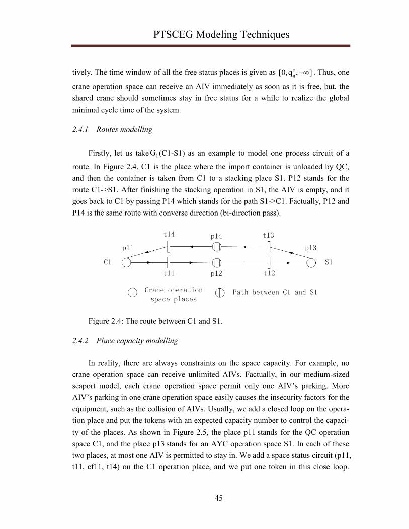
PTSCEG Modeling Techniques
45
tively. The time window of all the free status places is given as e
ij[0,q , ] . Thus, one
crane operation space can receive an AIV immediately as soon as it is free, but, the
shared crane should sometimes stay in free status for a while to realize the global
minimal cycle time of the system.
2.4.1 Routes modelling
Firstly, let us take 1G (C1-S1) as an example to model one process circuit of a
route. In Figure 2.4, C1 is the place where the import container is unloaded by QC,
and then the container is taken from C1 to a stacking place S1. P12 stands for the
route C1->S1. After finishing the stacking operation in S1, the AIV is empty, and it
goes back to C1 by passing P14 which stands for the path S1->C1. Factually, P12 and
P14 is the same route with converse direction (bi-direction pass).
Figure 2.4: The route between C1 and S1.
2.4.2 Place capacity modelling
In reality, there are always constraints on the space capacity. For example, no
crane operation space can receive unlimited AIVs. Factually, in our medium-sized
seaport model, each crane operation space permit only one AIV‟s parking. More
AIV‟s parking in one crane operation space easily causes the insecurity factors for the
equipment, such as the collision of AIVs. Usually, we add a closed loop on the opera-
tion place and put the tokens with an expected capacity number to control the capaci-
ty of the places. As shown in Figure 2.5, the place p11 stands for the QC operation
space C1, and the place p13 stands for an AYC operation space S1. In each of these
two places, at most one AIV is permitted to stay in. We add a space status circuit (p11,
t11, cf11, t14) on the C1 operation place, and we put one token in this close loop.

PTSCEG Modeling Techniques
46
Then, there is at most one token in p11 by the control of the synchronized transition
t14. For the place S1, we can add the space status circuit (p13, t13, sf11, t12) to con-
trol the number of tokens in S1.
Figure 2.5: Place capacity modeling by PTSCEG.
The place cf11 is a free status place of p11, which means the operation space of
C1 is empty and can be used immediately if necessary. And sf11 plays the same role
for place p13. For the places p12 and p14, since the space of the route is big enough
for the available AIVs, so, we don‟t need to add the close loops or the space status
circuits to control the capacity.
More generally, for a system which can be expressed as a PTSCEG, if the capac-
ity of one place should be limited, it is possible to add a close loop with the free status
place of this place, and put the tokens with the demanded capacity number in the
close loop, to control the token number.
2.4.3 Shared crane operation space modelling
Let us take S1 as an example to show how to model a shared crane space. As
shown in Figure 2.6, the shared space status circuit of S1 is constituted by two free
status places sf11 and sf12, and two busy status places, p13 and p23. The tokens in
process circuits 1G (C1-S1) and 2G (C2-S1) represent the AIVs, and the token in the
shared space circuit represent the capacity to receive AIV in the confined shared
space. There is only one token in the S1 status circuit, which means only one AIV is
permitted to unload containers in S1 at any moment. Hence, we don‟t need to add the
capacity control circuits for p13 and p23.

PTSCEG Modeling Techniques
47
Figure 2.6: The shared crane space S1 with two routes modeled by PTSCEG.
The close loop of shared space status (p13, t13, sf12, t22, p23, t23, sf11, t12)
connects the two process circuits 1G and 2G . The capacity of operation space S1 is
controlled by the number of tokens in the shared space status circuit and the syn-
chronized transitions t12 and t22. Only one token can appear in either p13 or p23 or
the free status, and it is impossible to observe the token appear p13 and p23 at the
same time. Thus, the shared space status models well the operation status of the
shared cranes of different container transit paths.
More generally, for any shared space of a system which can be expressed as a
PTSCEG, it is possible to add a shared space status circuit and put the limited capaci-
ty number of tokens in this circuit to model the shared space with demanded capacity.
2.4.4 Intersections modelling
The intersections are more complex to be modelled. As shown in Figure 2.7, in
an intersection point X1of two routes 3G (C2-S3) and 4G (C3-S2), the AIVs on the
same path will not restrict the passage for each other, but the existence of one AIV
will forbid the passage of AIVs on other crossing routes.

PTSCEG Modeling Techniques
48
Figure 2.7:The intersection X1 modeled by PTSCEG.
X1 is a shared intersection space of 3G and 4G . The shared space status circuit
can be used to control the number of tokens in X1. P33 and p37 stand for the X1
space on the route C2-S3 with converse direction. P43 and p47 stand for the X1 space
on the route C3-S2 with converse direction. As we have assumed, in the intersections,
the AIVs only forbid the passage of AIVs of other routes. So, p33 is a shared space
place for p43 or p47, and p37 is a shared space place for p43 or p47. There are 4
shared space status circuits in Figure 2.7, such as
(p33, t33, xf15, t42, p43, t43, xf14, t32)
(p33, t33, xf16, t46, p47, t47, xf13, t32)
(p37, t37, xf12, t42, p43, t43, xf17, t36)
(p37, t37, xf18, t46, p47, t47, xf11, t36)

PTSCEG Modeling Techniques
49
xf11, xf12, xf13, xf14, xf15, xf16, xf17 and xf18 are 8 free status places for X1.
Let us put one token in each of the 4 shared space status circuits. If there are to-
kens in p33 or p37 (p43 or p47), no token can enter into p43 or p47 (p33 or p37). By
this control, the AIVs are much safer while passing the intersections. The AIVs are
intelligent to avoid the collisions between each other on the routes with the same or
converse direction, but it is still difficult for AIVs to deal with the location problem
while facing AIVs from more than 3 directions (in the intersection point) in the same
time. However, the intersection is a highly dynamic and complex environment for
AIVs. So, the control on the intersections is necessary for reducing the collision prob-
ability of AIVs.
Moreover, the intersection control technique presented here may be extended to
the intelligent traffic light control system. The cars on the route can be seen as AIVs,
and the passage rule of cars on a crossroads is very similar to the restriction relation
of AIVs in the intersection point.
2.4.5 Ratio-driven task modelling
For a real transportation task, the number of the containers transited on each
route is not obliged to be equal. There is always a known transportation ratio for the
different routes.
We suppose that:
• the transit ratio of containers on route i is given by ir with, ir 1 ,
• there exists a set of positive integers if with no common divisor greater than
1 and such that i i ir f / f .
There are two modelling techniques to model the ratio-driven task, Hillion-like
method and Ohl-like method.
2.4.5.1 The Hillion-like modelling technique
In (Hillion and Proth, 1989), a method to model the ratio-driven job shop system
is presented. Their work is based on T-timed event graphs. The main idea of (Hillion
and Proth, 1989) is to make the if same process circuits in parallel, and to connect the
all the process circuits with shared machines.
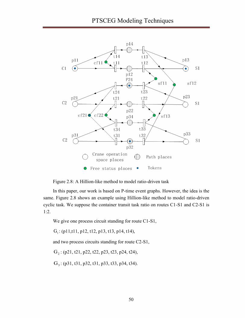
PTSCEG Modeling Techniques
50
Figure 2.8: A Hillion-like method to model ratio-driven task
In this paper, our work is based on P-time event graphs. However, the idea is the
same. Figure 2.8 shows an example using Hillion-like method to model ratio-driven
cyclic task. We suppose the container transit task ratio on routes C1-S1 and C2-S1 is
1:2.
We give one process circuit standing for route C1-S1,
1G : (p11,t11, p12, t12, p13, t13, p14, t14),
and two process circuits standing for route C2-S1,
2G : (p21, t21, p22, t22, p23, t23, p24, t24),
3G : (p31, t31, p32, t31, p33, t33, p34, t34).

PTSCEG Modeling Techniques
51
The three process circuits 1G , 2G and 3G are connected by the shared space sta-
tus circuits:(p13, t13, sf12, t32, p33, t33, sf13, t22, p23, t23, sf11, t12) and (p21, t21,
cf22, t34, p31, t31, cf21, t24).
3G is just a repeat of 2G , and all the process circuits are connected into parallel
type. By this kind of modeling, per cycle time, one container can be transited on route
C1-S1, and two containers can be transited on route C2-S1.
2.4.5.2 The OHL-like modelling technique
Figure 2.9: An OHL-like method to model the ratio-driven task.
In (Ohl et al., 1995), the authors gave a new modelling technique for the ratio-
driven job-shop problems. Their work is also based on T-timed event graphs. The
main idea in (Ohl et al., 1995) is to make the if same process circuits in series, and to
connect the all the process circuits with shared machines.
We apply this idea on the PTSCEG model, as shown in Figure 2.9.
The route C1-S1 is expressed by one process circuit,
1G : (p11,t11, p12, t12, p13, t13, p14, t14).

PTSCEG Modeling Techniques
52
And the route C2-S1 is expressed by one process circuit repeating twice the con-
tainer transit procedures in series,
2G : (p21, t21, p22, t22, p23, t23, p24, t24, p25, t25, p26, t26, p27, t27, p28,
t28).
The two process circuits 1G and 2G are connected by the shared space status cir-
cuits (p13, t13, sf11, t26, p27, t27, sf13, t22, p23, t23, sf12, t12). By this kind of
modeling, we can also realize transporting one container d on route C1-S1 and two
containers on route C2-S1 per cycle time. If the cycle time is fixed, the lower bound
of token number using OHL-like method is better than the Hillion-like method. The
comparison of these two methods will be discussed in section 2.5 of Chapter 2
2.4.6 The complete container transit PTSCEG model
In the above sections, the PTSCEG is used to model the routes, the crane opera-
tion spaces, the intersections, the shared operation spaces and the ratio-driven task.
Thus, a complete container transit procedure in the sketch map (Figure 2.3) can be
expressed by a PTSCEG. Figure 2.10 shows the container transit procedures on 10
routes which are connected by the shared operation spaces.
We suppose that the container transit ratio on each route i is ir 0.1 , if 1 , for
i=1…10. In other words, the number of containers transited on each route is equal.
The hypothesis for the equal ratio does not lose the generality. Factually, our robust
cyclic scheduling techniques are based on a theoretical semantic analysis of PTSCEG.
The ratio-driven modelling technique in section 2.4.5 is used for give suitable
PTSCEG model for ratio-driven task. Whatever the ratio is, as long as the ratio-driven
task can be modelled as PTSCEG, we can apply the robust cyclic scheduling on it.
In the complete PTSCEG container transit model,
1G (C1-S1) and 2G (C2-S1) are connected by the shared space status circuit of
the AYC operation space S1,
2G (C2-S1) and 3G (C2-S3) are connected by the shared space status circuit of
the QC operation space C2,
3G (C2-S3) and 4G (C3-S2) are connected by the shared space status circuits of
the intersection space X1,

PTSCEG Modeling Techniques
53
Figure 2.10: The complete PTSCEG model of the import container transit proce-
dures.

PTSCEG Modeling Techniques
54
4G (C3-S2) and 5G (C3-S4) are connected by the shared space status circuit of
the QC operation space C3,
5G (C3-S4) and 7G (C5-S4) are connected by the shared space status circuit of
the AYC operation space S4,
6G (C4-S5) and 7G (C5-S4) are connected by the shared space status circuits of
the intersection space X2,
6G (C4-S5) and 8G (C5-S5) are connected by the shared space status circuit of
the AYC operation space S5,
7G (C5-S4), 8G (C5-S5) and 9G (C5-S6) are connected by the shared space sta-
tus circuit of the QC operation space C5,
9G (C5-S6) and 10G (C6-S6) are connected by the shared space status circuit of
the AYC operation space S6.
From the modelling steps, it is noticed that the PTSCEG has some advantages,
such as,
• it captures the precedence relations of the operations,
• it avoid the conflicts of the use of the shared resources,
• it avoid the confusion of the AIVs to choose the routes,
• the time windows can be modelled easily,
• the space capacity can be modelled easily.
Moreover, the PTSCEG has a well-developed mathematical and practical foun-
dation, and the lower or upper bound of the cycle time or the number of the tokens in
process circuits can be given by the special properties of PTSCEG.
These advantages will be very useful in the work for the MIP modelling and the
robust control technique. The section 2.5 will present the cutting techniques by using
the special properties of PTSCEG. And these cutting techniques will be used in Chap-
ter 3 for reducing the research space of MIP mathematical model.

PTSCEG Modeling Techniques
55
2.5 Cutting techniques
As discussed in the section 1.3.2, the cutting techniques used in (Hillion and
Proth, 1989, Bourdeaud'Huy and Korbaa, 2006, Ben Amar et al., 2007, Ben Amar et
al., 2010b, Ben Amar et al., 2010a, Ben Amar et al., 2011) are shown, including the
lower bound of the cycle time, the upper bound of the cycle time, the lower bound of
the WIP number and the upper bound of the WIP number. In their works, the consid-
ered examples are the job-shop problems based on T-timed event graph. Thus, the
operation time is a fixed duration rather than a changeable time window. And only
the operation time on machines is taken into account, the transporting time of prod-
ucts among machines is ignored. But in this thesis, we use the PTSCEG which is a
kind of strongly connected event graph with time windows. With PTSCEG, the op-
eration time can be changeable in a time window, and the transporting time can be
considered into the modeling. Based on the cutting techniques of T-timed event graph,
we introduce some cutting techniques of PTSCEG as the follows.
2.5.1 The bound of the cycle time
In (Khansa et al., 1996b, Khansa et al., 1996a), the authors discussed the interval
of the possible cycle time of a PTSCEG. It is known that a PTSCEG can be decom-
posed into several elementary circuits (see Definition 2.5). And each place of the el-
ementary circuit has a time window ij ij[a ,b ] to bound the sojourn time of tokens in it.
Thus, the cycle time of an elementary circuit iG is
iJ
ij1i
i
qC
W
, which is located
in the interval i iJ J
ij ij1 1
i i
a b[ , ]
W W
.
The lower bound of cycle time ofG is
iJ
ijmin 1
i
aC max
W
(2.1)
s.t. i iJ J
ij ij1 1i
i i
a b[ , ]
W W
The upper bound of cycle time of G is

PTSCEG Modeling Techniques
56
iJ
ijmax 1
i
bC min
W
. (2.2)
s.t. i iJ J
ij ij1 1i
i i
a b[ , ]
W W
The lower bound of cycle time is usually used, which stands for the optimal
productivity of the manufacturing activities. But the upper bound also makes sense in
the real industrial activity. For example, a regular maintenance is given on a produc-
tion line. We can insert the maintenance by degrading the performance of system with
cycle time at least less than the upper bound. If the insert of the maintenance makes
the cycle time bigger than the upper bound, then we should stop the system complete-
ly. The upper bound of cycle time gives us the worst performance of the system with
the most degraded productivity without totally being suspended. However, sometimes,
a degraded performance is better than completely stopping the system.
2.5.2 The bound of tokens with demanded cycle time
The number of tokens in process circuits has its physical meaning for job-shop
problems or container transit procedures. For the job-shop problems in (Hillion and
Proth, 1989, Ohl et al., 1995), the number of tokens in the process circuits stands for
the number of the pallets for supporting the products. In our work, the number of to-
kens in the process circuits stands for the number of AIVs. It is always expected to
realize the demanded cycle time with the least transport resources. Especially, in the
container transit activities, the transport resource AIVs are very expensive. It is really
interesting to use less AIVs to do the container stevedoring respecting the demanded
delivery time. However, the upper bound of AIVs is not interesting for us, so it is not
discussed in this work.
The main idea of (Hillion and Proth, 1989) is to make the same product process
circuits in a parallel style, and the idea of (Ohl et al., 1995) is to make the same prod-
uct process circuits in a series style. The lower bound of token number in (Ohl et al.,
1995) is better than the lower bound in (Hillion and Proth, 1989). But all their works
are based on T-timed event graph and the operation time can‟t be changed. We apply
their ideas in PTSCEG with some necessary modifications.

PTSCEG Modeling Techniques
57
For a demanded cycle time demandC , the minimal number of tokens in circuits
using Hillion-like method is,
ij
1 i
i demand
qB f
C
(2.3)
and the minimal number of tokens in circuits using OHL-like method is,
ij
2 i
i demand
qB f
C
(2.4)
Obviously we have 2 1B B . It is important to recognize that 1B and 2B are two
bounds based on exactly the same assumptions about the transport system. The defi-
nition of ijq and if can be found in the pages 37 and 43.
The cutting techniques in (2.1), (2.2), (2.3) and (2.4) will be
used in Chapter 3 for reducing the researching space or reducing the computing time
of Mixed Integer Programming (MIP) models.
2.6 Conclusion
In this chapter, for the container transit procedures, it is demonstrated that the
PTSCEG can well model the time windows, the routes, the shared crane operation
space, the intersections, and the ratio-driven task. Compared to the job-shop problems
which appear in many articles (Collart-Dutilleul et al., 2007, Mhalla et al., 2008, Jerbi
et al., 2009, Collart-Dutilleul et al., 2013, Mhalla et al., 2013a, Mhalla et al., 2013b),
the PTSCEG is firstly used to model container transit in this thesis. As each place in
PTSCEG has just one input arc and one output arc, there is no conflict. So, for the
AIV staying in a confined space or on the route, there is no choice confusion for en-
tering the next space, which implies the control complexity of the AIV group is re-
duced by the inherent property of event graph.
Moreover, the bound of cycle time and token number can be given for a
PTSCEG model, which can be used as cutting techniques in the Chapter 3 . The cycle
time is the inverse of productivity, and the token number in the process circuits stands

PTSCEG Modeling Techniques
58
for the AIV number. In Chapter 3 , two objective functions will be given for the MIP
model. One is to minimize the cycle time to realize the maximal productivity, and the
other is to minimize the token number to reduce the AIV group control complexity
and energy cost.
The PTSCEG container transit model given in this chapter is also a graphical
base for the MIP mathematical model and the robust control algorithms. This com-
plete model is often mentioned in the following chapters.

MIP Modeling Techniques
59
Chapter 3 Mixed Integer Programming (MIP)
modeling techniques for cyclic scheduling
In Chapter 2, the container transit PTSCEG modeling technique is presented. In
a PTSCEG model, two kinds of elementary circuits exist, process circuit and space
status circuit. The close loop (the elementary circuit) guarantees an inherent ad-
vantage to describe the cyclic scheduling. As the cyclic scheduling is NP-hard, the
heuristic methods are used in many researches. But the heuristic methods may lead a
long computing time and non-optimal solutions. Here, we introduce a simpler but ef-
ficient method to model and compute the 1-cyclic schedule. Based on the structure of
the PTSCEG model, the MIP is used to describe the activities of tokens in one cycle
time. Then, the constraints are programmed directly in CPLEX for cyclic scheduling.
This method avoids the heavy workload of heuristic programming. For scheduling the
container task in a medium sized container terminal, this method may be more ac-
ceptable for the technicians and manager of seaport. The transient period of cyclic
scheduling is neglected considering the very short time compared with the steady
state of cyclic schedule.
This chapter concentrates on the MIP modeling techniques for 1-cyclic schedul-
ing of container transit procedures in a medium sized seaport. Since the operations
executed on the machines of 1-cyclic scheduling repeat once per cycle time, so it
needs just to study the constraints for the operations in one cycle time without losing
the generality. Firstly, the constraint families for different kinds of places are pre-
sented. Then, the complete MIP models for minimizing the cycle time and the token
number are given. Thirdly, based on the given time windows for each place in the
complete PTSCEG model, the expected sojourn time within time windows for the cy-
clic schedule is achieved by MIP models with cutting techniques. The efficiency of the
cutting techniques is also discussed in this chapter.

MIP Modeling Techniques
60
3.1 The constraint family explanation
In the Chapter 2 , the container transit process is modeled by PTSCEG. This
kind of model can clearly present the precedence relations of operations in the con-
tainer transit process, and can easily model the time windows. Based on the PTSCEG
model, in this chapter, the MIP mathematical model is used to calculate the expected
sojourn time in time windows. For 1-cyclic scheduling, the activities are repetitive in
one cycle time C . So it just needs to study the processing activities in one cycle time
instead of considering the activities in the whole production period. However, the
computing time of a schedule in one cycle time C is much smaller than a schedule
for the whole production period. Thus, the expected sojourn time can be computed in
a short time. Three kinds of constraint families are presented here: general constrains
for all the places; constraints of places in the process circuits; constraints of places in
the shared space status circuits.
The notions used in this chapter is exactly the same as given in the section 2.3 .
• G: the PTSCEG model
• iG : ith elementary circuit represents the process circuit or the space status
circuit, i N
• ijp : jth place of iG , the places stand for the operation space of QCs, AYCs,
the intersections, the paths, and the free status of a shared space j N
• ijt : jth transition of iG
• o o
ij ijp (p ) : the input (output) transition of ijp
• ilV : the l th token for iG , Nl
• ijs : entering date of one token in ijp , ijs 0
• ijq : the sojourn time of one token in ijp , ijp 0
• e
ijq : the expected sojourn time of tokens to realize the demanded cycle time
of system, e
ijq 0

MIP Modeling Techniques
61
• ija : the lower bound of
ijq ,ija 0
• ijb : the upper bound of ijq , ijb 0
• W : total number of tokens in G , W N
• iW : the number of tokens in iG , iW N
• limitW : the limit number of tokens in G ,
limitW N
• limit
iW : the limit number of tokens in iG , limit
iW N
• C : variable stands for cycle time of G , C 0
• iC : variable stands for cycle time of circuit iG , iC 0
• minC : the minimal cycle time of G ,
minC 0
• maxC : the maximal cycle time ofG ,
maxC 0
• I : I max i , the number of iG
• iJ : number of places of iG
• ij : Boolean variable
• ' 'i j
ij : Boolean variable
3.1.1 Constraints on all the places
Since the model is a PTSCEG, a time window ij ij[a ,b ] should be assigned on
every place ijp . The ija is the lower bound of the sojourn time of tokens, and ijb is the
upper bound. In an elementary circuit iG of G , ijp is the jth place, and ijq is the sojourn
time of tokens in ijp . The ijq in the place ijp is taken into account in transition valida-
tion when it has stayed in ijp for duration of at least ija and at most ijb . After the dura-
tion ijb the token will be dead. The constraint family (3.1) describes the semantic defi-
nition of PTSCEG.

MIP Modeling Techniques
62
ij ij ija q b (3.1)
Let us take the activities of tokens in elementary circuit 2G as an example. C2 is
its first place. 2G :(p21, t21, p22, t22, p23, t23, p24, t24), it is presented in Figure 3.1,
and the time windows are also given. For each place, let us denote ij ij[a ,b ] the lower
bound of the time window, and the upper bound of the time window, respectively.
Figure 3.1: A PTSCEG with time windows
As shown in Figure 3.1, two tokens (t21 and t22) are put into 2G . It is possible
to give a 1-cyclic schedule for the activities of tokens in 2G by the Gantt chart as
shown in Figure 3.2.
In Figure 3.2, the cycle time of 2G is 270, and all the sojourn time of the two to-
kens in all the places are located in the relative time windows. For example, the so-
journ time of token V21 in P24 is 145, and it is located in the time window [100,300].

MIP Modeling Techniques
63
Figure 3.2: The Gantt chart for 1-cyclic schedule in 2G .
In (1.1), the cyclic scheduling is defined as x n + k = x n + k*C for
n N,k N ,C 0 , x(n) is the starting time (or ending time ) of one activity, and n
means the repeat numbers. In our work, we suppose k=1. The cyclic scheduling we
study is so called 1-cyclic scheduling. Thus, all the activities of the tokens in the
place will repeat one time per cycle time C. So it just needs to study the processing
activities in one cycle time instead of considering the activities in the whole produc-
tion make-span. Thus, the constraint family (3.2) can be given as follows,
ij0 s C (3.2)
To explain constraint family (3.2), let us also take the activities of tokens in ele-
mentary circuit 2G as an example. This constraint family means that the arriving
time of one token in a place is located in [0, C). As shown in Figure 3.3, the cycle
time of 2G is 270. So, the entering time for each place is located in [0, 270).
21s 145 ,
22s 235 ,
23s 90 ,
24s 0 .
The constraint families (3.1) and (3.2) should be respected in any place of a
PTSCEG, no matter this place is in process circuit or the space status circuits. But

MIP Modeling Techniques
64
there are still some different special constraints which should be respected individual-
ly by the places in different kinds of circuits.
Figure 3.3: The arriving time of tokens in the places.
3.1.2 Constraints on places in the process circuits
iij ij iji j%J +1
s +q s = β- C (3.3)
iJIlimit
ij
1 1
W W (3.4)
In our example, there are two kinds of elementary circuits: process circuits and
space status circuits. Here, we use the activities of tokens in 2G to explain the con-
straints of 1-cyclic scheduling for tokens in the process circuits. Two constraint fami-
lies are given, (3.3) and (3.4). Here, % means the modulus operator, which can con-
nect all the places in the process circuit as a cycle (Bourdeaud'Huy and Korbaa, 2006),
while ijβ is a Boolean variable.
Constraint family (3.3) gives the precedence constraint of token‟s sojourn time
in two consecutive places. The complementation % in (3.3) connects the two succes-
sive places, including the last place and the first place. For example, the following
place of 24p is 21p which can be presented as 2 4%4+1
p . And ijβ stands for the number
of crossed cycles of ijq .

MIP Modeling Techniques
65
Let us take the activities in 23p and 24p as an example to explain constraint
family (3.3), as shown in Figure 3.4.
23 23 23 23 23 24 232 3%4+1s +q s = β C s +q s = β C 90+180-0 = 2- * 70- 1
When the sojourn time in a place crosses one cycle time, it needs to add a token
in the circuit to reduce the cycle time. So the sum of ijβ is the total number of tokens
in the process circuit, as shown in (3.4). For example, in Figure 3.4, there are 2 tokens,
21v and 22v , and the sum of 2 j is 0+0+1+1=2. However, the total number of tokens
should be less than the limited number of tokens. In other words, the number of used
AIVs in system should be less than the number of all the AIVs.
Figure 3.4: Boolean variable ij determines the tokens number.
3.1.3 Constraints on places in the space status circuits
In the above section 3.1.2, we have discussed the constraint families about the
sojourn time and the arriving time of tokens in the process circuits in just one cycle
time C. In this section, the constraint families about the activities of tokens in the
space status circuits are studied.
In a PTSCEG model as shown in Figure 3.1, there are two kinds of space status
circuits, one kind is the non-shared space status circuit, and the other kind is the
shared space status circuit. In Figure 3.1, (p11, t11, cf11, t14) and (p21, t21, cf21, t24)
are two non-shared space status circuit, and (p13, t13, sf12, t22, p23, t23, sf11, t12) is
a shared space status circuit for process circuits 1G and 2G .
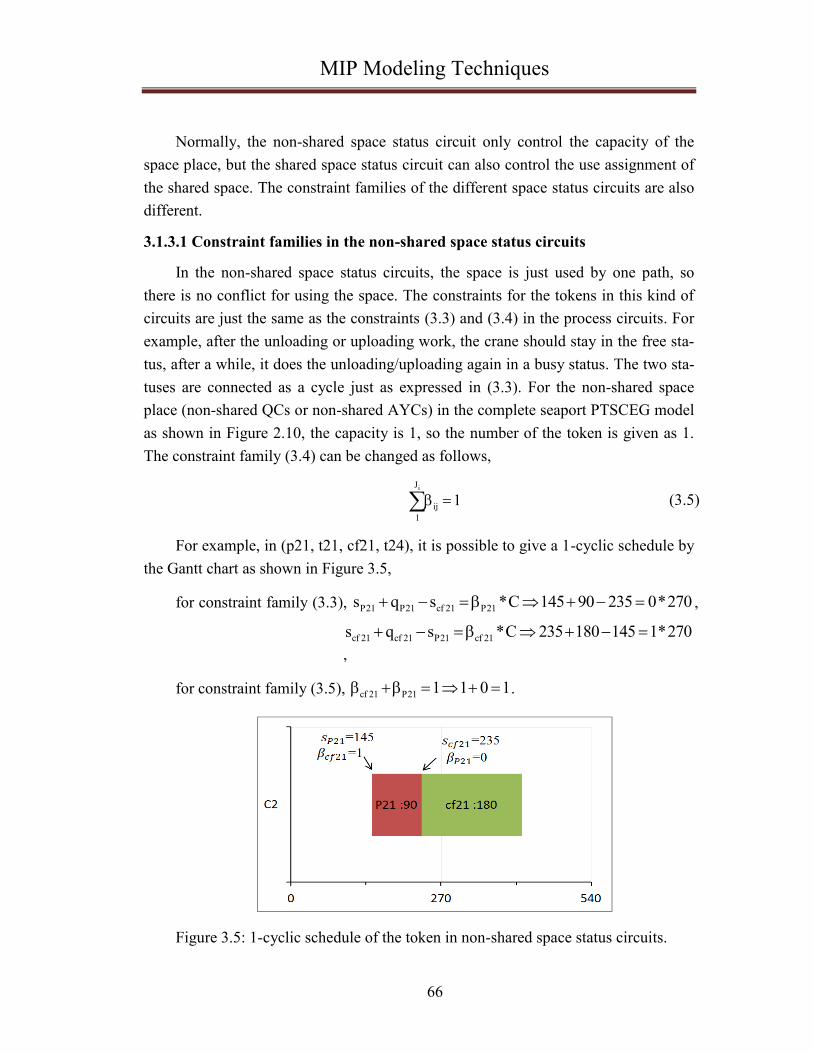
MIP Modeling Techniques
66
Normally, the non-shared space status circuit only control the capacity of the
space place, but the shared space status circuit can also control the use assignment of
the shared space. The constraint families of the different space status circuits are also
different.
3.1.3.1 Constraint families in the non-shared space status circuits
In the non-shared space status circuits, the space is just used by one path, so
there is no conflict for using the space. The constraints for the tokens in this kind of
circuits are just the same as the constraints (3.3) and (3.4) in the process circuits. For
example, after the unloading or uploading work, the crane should stay in the free sta-
tus, after a while, it does the unloading/uploading again in a busy status. The two sta-
tuses are connected as a cycle just as expressed in (3.3). For the non-shared space
place (non-shared QCs or non-shared AYCs) in the complete seaport PTSCEG model
as shown in Figure 2.10, the capacity is 1, so the number of the token is given as 1.
The constraint family (3.4) can be changed as follows,
iJ
ij
1
1 (3.5)
For example, in (p21, t21, cf21, t24), it is possible to give a 1-cyclic schedule by
the Gantt chart as shown in Figure 3.5,
for constraint family (3.3), P21 P21 cf 21 P21 145 90 235 0s q s **C 270 ,
cf 21 cf 21 P21 cf 21 235 180 145 1*s q s *C 270
,
for constraint family (3.5), cf 21 P21 1 1 0 1 .
Figure 3.5: 1-cyclic schedule of the token in non-shared space status circuits.

MIP Modeling Techniques
67
3.1.3.2 Constraint families in the shared space status circuits
It is should be noticed that, if a space place is just shared by two process circuits,
then, the constraint families (3.3) and (3.5) are still suitable to determine the activities
of the token in the shared space status circuit. Let us take the shared space circuit of
S1 (p13, t13, sf12, t22, p23, t23, sf11, t12) as an example. As shown in Figure 3.6,
(p13, sf12, p23, sf11) or (p23, sf11, p13, sf12) are the same cycle, and the constraint
families (3.3) and (3.5) can be well applied to determine the 1-cyclic schedule of the
token in this circuit.
Figure 3.6: 1-cyclic schedule in the shared space status circuit of S1.
Figure 3.7: The shared space status circuit of C5

MIP Modeling Techniques
68
But if the space place is shared by more than two process circuits, the constraint
families (3.3) and (3.5) lose the generality. Let us take the shared space C5 as an ex-
ample, as shown in Figure 3.7. It is a part of the complete PTSCEG model in Figure
2.10. The space C5 is shared by three process circuits, 7G (C5 S4) , 8G (C5 S5)
and 9G (C5 S6) . The cycle (p71, p81, p91) as shown in the figure is different with
the cycle (p71, p91, p81). However, the cycle (p71, p81, p91) and the (p71, p91, p81)
are both two possible solutions to optimize the 1-cyclic schedule. It is not reasonable
to use only one possible space status cycle to optimize the cycle time. The order to
use the space C5 for different process circuits should be a degree of freedom. The
constraint families (3.3) and (3.5) can only be applied to a given cycle, but they are
not suitable for a cycle in which the order of the places is not fixed.
f
ij
i j
ij ij i j ijs q sa C
(3.6)
f i j
i j i j i j ij ijs q Ca s 1 *
(3.7)
Constraint families (3.6) and (3.7) present the no overlap relation of the opera-
tions in places ijp and i jp which stand for the same shared space busy status. The
shared space can only be used by at most one process circuit at any moment. i j
ijγ
is a
Boolean variable. f
ija is the lower bound of the free status after the operation in ijp . It
is should be noticed that the time window of the free status of cranes is [0, + ] as
shown in Figure 3.7. So the sojourn time of token in P71 and P81, P81 and p91, P91
and P71 can be connected directly, if the sojourn time in free status place equals 0.
Figure 3.8: 1-cyclic schedule of the token in the shared space circuit of C5.

MIP Modeling Techniques
69
In Figure 3.8, a possible 1-cyclic schedule of the token in the shared space status
circuit of C5 is given. Let us take P71 and P81 as an example.
81
71 0 , 71
81 1 , f
71a 0 , f
81a 0
f
71 71 71 81s q a s 55 90 0 145 0 0 C
f
81 81 81 71s q a s 145 90 0 55 180 1 0 *C
Some constraint families similar with (3.6) and (3.7) have been discussed in (Seo
and Lee, 2002) and (Bourdeaud'Huy and Korbaa, 2006). But in their works, the prob-
lems are modeled as timed Petri nets and the sojourn time of tokens ijq can‟t be
changed. In our work, the sojourn time ijq is changeable in a time window [ ij ija ,b ],
which is more flexible than the work in (Seo and Lee, 2002) and (Bourdeaud'Huy and
Korbaa, 2006). Their work is not adaptable for our container transit procedures with
time windows and changeable operation durations.
3.2 The complete MIP models
In the above section 3.1 , the necessary constraints for 1-cyclic schedule have
been given. The objective functions are also important for a complete MIP model. In
the seaport container transit procedure, the number of the AIVs is limited, the capaci-
ty of resources (crane operation space and intersections of crossing routes) is limited,
and the processing time is bounded (the time window). With these limitations, for a
transit procedure manager, the minimal cycle time (the reciprocal of maximal produc-
tivity) is a very important criterion to evaluate the performance of system. One single
container transit can be finished in each process circuit (the routes) per cycle time.
The smaller the cycle time is, the sooner the transit job can be finished, hence the bet-
ter we can guarantee the delivery time of containers for their following destinations.
So the first objective function is to minimize the cycle time.
Obj 1: Minimize ( C ).
But sometimes, the admissible solution is not unique, that means it exists more
than one 1-cyclic schedule for AIVs to finish the job with the optimal cycle time. At
this situation, for the manager of the container transit, it is more interesting to finish
the job with less AIVs. The less AIVs we use, the less complex to control the AIVs

MIP Modeling Techniques
70
group it is. The free AIVs can be also seen as the reserve force to replace the used
AIVs with unpredictable breakdown. Moreover, considering the objectives of In-
TraDE project, it improves the clean production because we use as few AIV as we
can to finish the task with less energy cost whilst respecting the optimal cycle time.
So the second objective function is to minimize the used AIVs while respecting the
optimal cycle time.
Obj 2: Minimize ( iW ), with iG is a process circuit.
Based on the two objective functions, it is possible to give two kinds of MIP
models. One is the MIP model which aims to minimize the cycle time with the lim-
ited transport resources. The other one is the MIP model which aims to minimize the
AIVs number, when there are more than one admissible solution with the overall op-
timal cycle time.
3.2.1 The MIP model for minimizing the cycle time
………………………………………………………………………………….......
Minimize :C s.t.
……………………………………………………………………………………...
ii 1, I , j 1, J ,
……………………………………………………………………………………...
ij ij ija q b (3.8)
ij0 s C (3.9)
……………………………………………………………………………………...
iG is a process circuit or a non-shared space status circuit,
iij ij iji j%J +1
s +q s = β- C (3.10)
……………………………………………………………………………………...
iG are the process circuits,

MIP Modeling Techniques
71
iJIlimit
ij
1 1
W W (3.11)
……………………………………………………………………………………...
iG is a non-shared space status circuit,
iJ
ij
1
1 (3.12)
……………………………………………………………………………………..
iG is a shared space status circuit,
i j
ij ij i j ijs q s C
(3.13)
i j
i j i j ij ijs q s 1 *C
(3.14)
………………………………………………………………………………….......
In the above MIP model, we suppose the lower bound of the free status of shared
space is zero. So the f
ija is neglected in (3.13) and (3.14).
And for the process circuits and the non-shared space status circuits, they use the
same constraint family (3.10) to determine the arriving time and sojourn time of to-
kens. But they use the different constraint families to determine the token numbers in
these circuits. For the process circuits, (3.11) implies that the number of the used
AIVs on all the routes should be less than the number of all the AIVs. The number of
AIVs on the single route is not very interesting for the manager of container transit.
For each non-shared crane operation space circuit, the capacity to receive AIV should
be 1 just as expressed in (3.12).
3.2.1.1 Lower bound of cycle time
The lower bound of the cycle time can directly referred to (2.1) as,
iJ
ijmin 1
i
aC C max
W
(3.15)
The upper bound of the cycle time can directly referred to (2.2) as,

MIP Modeling Techniques
72
iJ
ijmax 1
i
bC C min
W
(3.16)
3.2.1.2 The constraint number analysis
From (3.8) to (3.14), we have 7 constraint families.
Let us denote n the number of places in process circuits, h the number of the
non-shared status circuits, and m the number of shared spaces, and ml the number of
process circuits which share the thm space.
In total, the previous model contains:
• 2(n h) 1 integer variables,
• m
m m
1
l (l 1)n 2h
2
Boolean variables,
• m
m m
1
3(n 2h) 3 l (l 1) constraints.
3.2.2 The MIP model for minimizing the token number
If the optimal cycle time is found with more than one solution, the second objec-
tive function should be considered to minimize the number of used AIVs.
……………………………………………………………………………………...
iJI
ij
1 1
Minimize : , with iG is a process circuit, s.t.
……………………………………………………………………………………...
ii 1, I , j 1, J ,
……………………………………………………………………………………...
ij ij ija q b (3.17)
min
ij0 s C (3.18)
……………………………………………………………………………………...

MIP Modeling Techniques
73
iG is a process circuit or a non-shared space status circuit,
i
min
ij ij iji j%J +1s +q s = C- β (3.19)
……………………………………………………………………………………...
iG is a non-shared space status circuit,
iJ
ij
1
1 (3.20)
……………………………………………………………………………………..
iG is a shared space status circuit,
i j min
ij ij i j ijs q s C
(3.21)
i j min
i j i j ij ijs q s 1 *C
(3.22)
………………………………………………………………………………….......
In this model, the cycle time is not a variable, but a constant integer. minC is the
optimal cycle time obtained by MIP model in section 3.2.1. And the object is to min-
imize the token number in the process circuits which stands for the AIV number.
3.2.2.1 Lower bound of token number
The lower bound of the number of token can directly referred to
(2.4), as
iij
im
JI
ij
1 1in
i
af
C
, with iG is a process circuit (3.23)
If we consider the example in Figure 2.10, if equals 1 for all the process circuits.
Each path has the same task ratio ir 0.1 . On each route, the transit rate of containers
per cycle time is the same.
3.2.2.2 The constraint number analysis
Form (3.17) to (3.22), we have 6 constraint families.

MIP Modeling Techniques
74
Let us denote n the number of places in process circuits, h the number of the
non-shared status circuits, and m the number of shared spaces, and ml the number of
process circuits which share the thm space.
In total, the previous model contains:
• 2(n h) integer variables,
• m
m m
1
l (l 1)n 2h
2
Boolean variables,
• m
m m
1
3(n 2h) 1 l (l 1) constraints.
3.3 Case study of the seaport container transit
Table 3.1. Time windows of places in process circuits
Circuits without in-
tersections Time windows
G1(C1⟷S1) p11[90,180] p12[90,300] p13[90,180] p14[100,300]
G2(C2⟷S1) p21[90,180] p22[90,600] p23[90,180] p24[100,600]
G5(C3⟷S4) p51[90,180] p52[90,400] p53[90,180] p54[100,400]
G8(C5⟷S5) p81[90,180] p82[90,600] p83[90,180] p84[100,600]
G9(C5⟷S6) p91[90,180] p92[90,500] p93[90,180] p94[100,500]
G10(C6⟷S6) p101[90,180] p102[90,600] p103[90,180] p104[100,600]
Circuits with inter-
sections Time windows
G3(C2⟷S3) p31
[90,180]
p32
[50,300]
p33
[5,10]
p34
[50,300]
p35
[90,180]
p36
[50,300]
p37
[5,10]
p38
[50,300]
G4(C3⟷S2) p41
[90,180]
p42
[50,280]
p43
[5,10]
p44
[50,280]
p45
[90,180]
p46
[50,280]
p47
[5,10]
p48
[50,280]
G6(C4⟷S5) p61
[90,180]
p62
[50,300]
p63
[5,10]
p64
[50,300]
p65
[90,180]
p66
[50,300]
p67
[5,10]
p68
[50,300]
G7(C5⟷S4) p71
[90,180]
p72
[50,270]
p73
[5,10]
p74
[50,270]
p75
[90,180]
p76
[50,270]
p77
[5,10]
p78
[50,270]
Let us apply the MIP models on the example shown in Figure 2.10. In a modern
container terminal, it takes about 2 minutes for cranes to finish loading or unloading
work. So the time window for QCs and AYCs can be set as [90,180] with the unit in
seconds. The distance between QCs and AYCs is supposed to be about 500 meters,
and the velocity of AIV is 5m/s. The time window for the AIVs to go along the routes

MIP Modeling Techniques
75
without intersections is [100, ijb ]. The AIV runs on the path with velocity 5m/s.
When it arrives at the end of the segment of one path, it should stay at the end until
the shared space is free. And a staying time on one path over more than ijb seconds is
not acceptable, and seen as a schedule failure. The value of ijb depends on the emer-
gency of the delivery time of containers. For the paths with intersections, the time
window for each path segment is [50, ijb
2], as the intersections are set in the middle
of route. And the time window of intersections is [5,10]. The time windows of places
in process circuits are shown in Table 3.1. The time window for the free status of op-
eration space place is [0, +∞], which means the cranes or intersections can be used
immediately if they are in free status, or they can stay in free status if no AIV is arriv-
ing.
Figure 3.9: The optimization strategy of MIP models.
As shown in Figure 3.9, the strategy to optimize the 1-cyclic schedule is to min-
imize the cycle time with the limited AIV number. Then, if more than one admissible
solution is found, the solution with the least AIV number should be chosen from all
the admissible solutions. In our model, each ship has 3000 containers, and 22 AIVs
are available to do the unloading work. Our aim is firstly to try to realize an optimal

MIP Modeling Techniques
76
cycle time, and then we want to use the least number of AIVs (less than 22 AIVs
maybe) to realize the optimal cycle time.
Moreover, it is expected that some operation space can be fully used without
waiting for the AIVs, which can be referred to the definition of bottleneck machine in
the section 1.3.2. In other words, some cranes are saturated without free status, then,
the overall maximal productivity is realized. The cyclic time of the system is con-
trolled by the most busy crane status circuits. By the structure analysis of the model in
Figure 2.10, the crane C5 can be saturated, and the status circuit of C5 is shared by
three process circuits, which gives the lower bound of optimal cycle time which is
90*3=270 seconds.
In this case, for the MIP model minimizing cycle time with limited AIV number,
we have: 123 integer variables, 83 Boolean variables, and 215 constraints; for the
MIP model minimizing AIV number with optimal cycle time, we have: 122 integer
variables, 83 Boolean variables, and 213 constraints. The CPLEX 12.5 is used to
make the simulation on a computer with Intel (R) Core (TM) i3-2310M at 2.10 GHz
and 4 Go RAM, under Window 7 (64 bit).
In Figure 3.10, Figure 3.11 and Figure 3.12, the 1-cyclic schedules for the AIVs
with the optimal cycle time C=270 are found, staying in the QCs operation space, in
the AYCs operation space and on the routes respectively.
The 20 used AIVs is less than the total 22 AIVs. It is sure that 20 is the minimal
number of AIVs to realize optimal cycle time. For example, if just 19 AIVs are used
in the schedule, it means one of the 10 routes can use just one AIV. The cycle time on
this route is at least 90+100+90+100=380 > 270 seconds, which is a paradox of the
optimal cycle time.
It should be noticed that the computing time of these schedules is about only 2
seconds. We also apply the MIP models on the job-shop problem discussed in the
section 2.1.2. The computing time is only about 0.1 second.
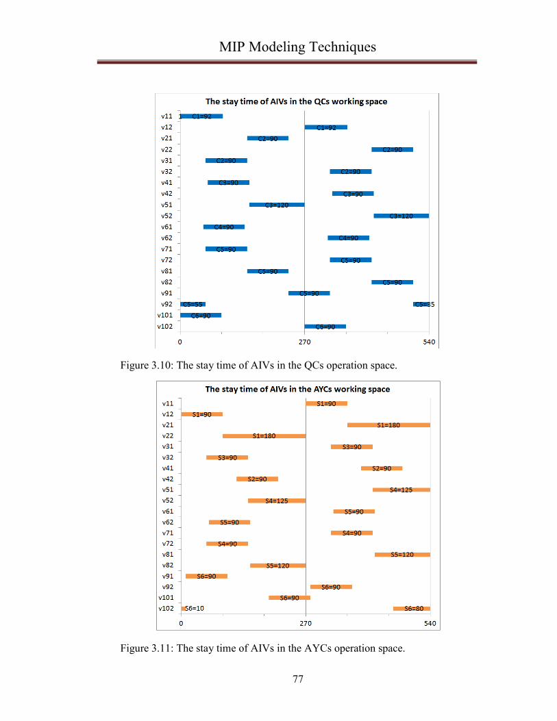
MIP Modeling Techniques
77
Figure 3.10: The stay time of AIVs in the QCs operation space.
Figure 3.11: The stay time of AIVs in the AYCs operation space.

MIP Modeling Techniques
78
Figure 3.12: The stay time of AIVs in the paths and the intersections.
Normally, all the location places of containers on ships and their stacking place
on the yard stacks can be known at least a few hours before the arrival of the vessels.
So, it is practical to apply this technique to give a 1-cyclic schedule for the container
transit task in advance. It is admitted that the transit routes should not be fixed in the
whole unloading period. During the entire transit task, some routes can be eliminated
if no more containers are transported to some stacks. If we consider the huge number
of containers on a ship, in one or two hours, the routes are fixed, so the 1-cyclic
schedule can be applied. Even if the routes are changed during the whole process, just
a few seconds are required to give a new cyclic scheduling. However, if we schedule
the whole process of unloading, it is possible to give a 1-cylic schedule class in a
short time. The 1-cylic schedule class is constituted by several 1-cyclic schedules ap-
plied to different period of the unloading work with the change of routes.

MIP Modeling Techniques
79
The very short computational time of the 1-cyclic schedule implies another ad-
vantage of the MIP model: if the disturbance in the system is outside of the system‟s
robustness margin, it is possible to reschedule a cyclic work plan in just a few se-
conds. The running duration of AIVs on routes and operation duration of cranes are in
minute time unit. So, the computing time of 1-cyclic scheduling can be neglected.
Reasonably, the 1-cyclic scheduling can be used as a reactive scheduling to resched-
ule in real time. The robustness margin means the range of disturbances which can be
rejected by a system‟s control without changing the actual schedule. More details
about active robustness margin are presented in the next chapter.
Table 3.2. Computing time of MIP model
Examples
(20 tests for each
example)
Route
number
AIV
number
Average computing time (s)
With lower
and upper
bounds
Without
upper
bound
Without
lower
bound
E1
Small
or me-
dium
sized
3 7 0.072 0.106 0.225
E2 5 15 0.608 0.697 >600
E3 6 17 1.002 1.304 >600
E4 7 19 1.463 1.476 >600
E5 8 20 1.514 28.860 >600
E6 9 21 1.982 >600 >600
E7 10 22 2.001 >600 >600
E8
Large
sized
11 23 5.530 >600 >600
E9 12 25 78.870 >600 >600
E10 13 27 >600 >600 >600
E11 14 29 >600 >600 >600
E12 15 31 >600 >600 >600
3.1 Analysis of computing time
Factually, the MIP models are also for different size of container transit task as
shown in Table 3.2.
If the container transit task studied is in a container terminal no bigger than a
medium size, the above table shows that the 1-cyclic schedule can be quickly found
in a few seconds with the lower and upper bounds of the cycle time. For a computing
time more than 600 seconds of MIP model without bounds, it is impossible to use the

MIP Modeling Techniques
80
relative schedule in real time as reactive scheduling, considering the operation dura-
tion and AIV running time in also in a few minutes.
Generally, there are three reasons for the efficiency of MIP method for 1-cyclic
scheduling:
• The considered example is at most a medium sized seaport, which limit the
number of constraints.
• We just need to consider the operations in one cycle time for 1-cyclic
scheduling, which reduces obviously the number of constraints compared to
non-cyclic scheduling. In the non-cyclic scheduling, we should study the
constraints of operations in the whole make-span.
• The lower and upper bound of objective function can be precisely defined
for the MIP models because of the inherent property of PTSCEG, which re-
duces obviously the searching space of the admissible solutions.
3.2 The comparison with other similar models
The models in (Seo and Lee, 2002, Bourdeaud'Huy and Korbaa, 2006, Ben
Amar et al., 2010b, Ben Amar et al., 2010a, Ben Amar et al., 2011) are very similar to
the seaport container transit model. However, they use examples less complex than
the container transit model as shown in Figure 2.10. In their example, the pallets allo-
cated to products are used to transport the job between machines, and the pallets will
only be removed from the products after completely finishing the job. The pallets in
their papers can be seen as the AIVs, the machines can be seen as the cranes, and the
containers can be seen as the products. We improved their work with simplified MIP
model structure and shorter computing time in (Zhang et al., 2014). The benchmark is
shown in the Appendices. But the MIP models in these papers are based on T-timed
Petri nets. The operation time of products on the machines is a fixed rational number.
The products can stay on the machine until the next needed machine is ready, which
implies the product can stay on one machine forever if the next machine is always
busy. By the T-timed Petri nets, the time windows of operations can‟t be appropriate-
ly assigned to the relative machine places. And the transportation time of products
among the machines are neglected in these works. For the container transit model in
this paper, it is not acceptable to let one AIV stay in one place for ever without lim-
ited upper time bound. The time windows of operation places and the transportation

MIP Modeling Techniques
81
duration should be both considered in our MIP models. We add the time window con-
straints and the transport resource constraints in work of (Zhang et al., 2014), then,
the MIP models adaptable to the container transit task are achieved in this chapter.
In (Brucker and Kampmeyer, 2008b), the authors try to give a general MIP
model for cyclic job shop with transportation robots. Actually, their model is just for
job shop problem of identical jobs and identical machines with only one transport ro-
bot. And the applied example is also very simple, with just 3 jobs and 3 machines. In
(Brucker et al., 2012), they give a modified MIP model for solving the cyclic job shop
problem with transportation. In this modified model, the number of the transport tool
is still only one. And they apply this model on an example with 10 jobs and 10 ma-
chines. But in our seaport model, it is not reasonable to use only one AIV for the con-
tainer transportation task. Factually, we have an AIV group. So the models in
(Brucker and Kampmeyer, 2008b, Brucker et al., 2012) can‟t be applied to our sea-
port model. Unfortunately, the models in (van Oostrum et al., 2008, Mannino et al.,
2012, Holte and Mannino, 2013) can‟t be applied to our seaport model too. They
mainly study the health-care problem.
Totally speaking, among the papers about cyclic scheduling in recent years, only
the works in (Seo and Lee, 2002, Bourdeaud'Huy and Korbaa, 2006, Ben Amar et al.,
2010b, Ben Amar et al., 2010a, Ben Amar et al., 2011, Zhang et al., 2014) are similar
to MIP models presented in this chapter. But these MIP models can‟t be applied to
our seaport container transit procedures, because they don‟t consider the time window
constraint of the machines and neglect the transport tools in their MIP models.
So it is impossible to make a benchmark of computing time with other cyclic
scheduling methods. But our MIP models still have some special features compared
to others,
• Our model includes the time window constraints: the models are based on
the semantic property of PTSCEG, and the time windows are assigned to the
crane operation space, the path and the intersections;
• Our model considers the transport tool: the AIVs are responsible to transport
the containers (not just one transport tool);
• Our model has a good performance to solve the medium sized seaport con-
tainer transit problem: the computing time is only about 2 seconds.

MIP Modeling Techniques
82
3.3 Conclusion
This chapter demonstrates that the MIP using CPLEX can be well applied to
compute the 1-cyclic schedule of container transit task in a medium sized seaport in a
short time. This method can be easily implanted in the real management of AIVs on
considering the good compatibility of CPLEX.
The information about the location of container in the vessels and in the yard
stacks can be known at least a few hours before the berthing of the vessels by the
quays. The MIP modeling technique needs just a few seconds to give a cyclic sched-
ule. So, the MIP modeling technique can be used as a predictable scheduling method
to schedule the cyclic container transit a few hours before the stevedoring. When the
stevedoring begins, the staying time of AIV on the routes or in the operation space is
about a few minutes. So, the computing time of rescheduling by MIP can be neglect-
ed if a delay/advance disturbance is observed. The MIP modeling technique can also
be seen as a reactive scheduling to reschedule the cyclic schedule in real time if nec-
essary.
The transient period of two cyclic scheduling is very short compared with the
steady state of cyclic scheduling. So, in our work, only the steady state is studied, and
the readers interested in the transient issues may consult (Bourdeaud'huy et al., 2011,
Calvez et al., 1998).

Robust Control Algorithms
83
Chapter 4 Robust Control for the 1-cyclic Sched-
uling
Using the MIP scheduling methods, it is possible to find a 1-cyclic scheduling in
short time. Thus, the expected sojourn time of AIVs in each place can be given
properly to realize the overall optimal productivity. Accordingly, the robustness algo-
rithms can be applied on the PTSCEG, which is based on the operation of sojourn
time and time windows. The algorithms have a computing time in polynomial com-
plexity, which makes it possible to compute the robustness margin on nodes of system
in short time as the 1-cyclic schedule is given. When the stevedoring begins, if one
disturbance is observed, we compare it with the robustness margin. If it is located in
the robustness margin, we can reduce or eliminate the disturbance by the robustness
algorithms. Moreover, for giving a better evaluation of the disturbance on all the
AIVs in system, a new robustness algorithm is proposed. This algorithm has a struc-
ture base in Gantt graph, and its computing time is also polynomial.
This chapter introduces three kinds of robust control algorithms for the 1-cyclic
scheduling of container transit task. The first kind and the second are directly based
on the structural control of the firing time of transitions in PTSCEG models. The
third is based on the control of the operation time of tokens in the Gantt graphs.
This chapter is basically organized as follows. Firstly, the two algorithms based
on the structure analysis of PTSCEG are introduced. Then we compare the two algo-
rithms in their computing complexity and the robustness margins. Thirdly, we intro-
duce a new algorithm based on the analysis of operations in Gantt graph. The details
about the compensable or transmissible margin of this new algorithm are well de-
fined by formulas. Finally, we compare the advantages and disadvantages of these
three algorithms.

Robust Control Algorithms
84
4.1 The algorithms based on the control of transitions
The above chapter proposes a 1-cyclic scheduling technique for container transit
process in a medium sized seaport. The achieved 1-cyclic schedule can just be applied
in an idealized work environment without any disturbance in the system, but the un-
predictable disturbances do exist in the real container terminal activities, such as the
delay or advance of AIVs or cranes. In this section, we propose algorithms to com-
pute the robust margin of each transition in PTSCEG to avoid the unnecessary alarm
due to disturbance which may cause the rescheduling of system. The system can re-
cover to initial normal status if the disturbance belongs to the robustness margin. As
presented in the Introduction section, all the AIVs and cranes can keep a real time
communication with a remote control center. This control center can get the exact po-
sition of each AIV by the signal points and can give a control signal to any AIVs or
cranes. The signal points can be seen as the transitions in PTSCEG. Thus, for the
PTSCEG model, it is reasonably supposed that each transition is observable and con-
trollable. In other words, it is possible to observe and control the sojourn time of each
token in any place by the output transition of this place.
4.1.1 Basic notation
Definition 4.1 (Collart-Dutilleul and Craye, 2003): Robustness is defined as the
ability of the system to remain valid with respect to the specifications when facing
some expected or unexpected variations. Robustness characterizes the global capacity
to deal with disturbances.
Definition 4.2 (Jerbi et al., 2004): A mono-synchronized sub-path Lp is a path
containing one and only one synchronization, which is its last node.
Definition 4.3 (Jerbi et al., 2004): An elementary mono-synchronized sub-path
is a mono-synchronized sub-path beginning with a place p such that o p is a synchro-
nization transition.
Definition 4.4 (Collart-Dutilleul et al., 2013): Temporal control is the modifica-
tion of the transition firing instants using a controlled P-time Petri net.
Definition 4.5 (Collart-Dutilleul et al., 2013): Active robustness is robustness
ensured by the temporal control of the process transitions.

Robust Control Algorithms
85
Definition 4.6: It is said that a transition t has a local active robustness on
min maxΔt ,Δt if the occurrence of a disturbance min maxt Δt ,Δt observed on t
does not involve a token death at t.
The local active robustness margin of t can be calculated using the following
formulas:
oij
e
min ij ijp =t
Δt = max a -q (4.1)
oij
e
max ij ijp =t
Δt = min b -q (4.2)
Figure 4.1: Case of local active robustness on a synchronized transition.
Example: Let us assume that a disturbance is observed on the synchronized tran-
sition 12t , as shown in Figure 4.1. Indeed,
12mint max 100 177,0 0 0
12maxΔt = min 300-177,+ =123
Consequently, there is no token death on transition 12t if a disturbance
t 0,123 is observed on 12t . For example, if a disturbance t 123 is observed
on 12t , it implies,
e
12 12 12q q t 177 123 300 b , and e
sf11 sf11 sf11q q t 0 123 123 b .
Thus, no token dies as the sojourn time is still located in the time windows. But,
if t 124 , then 12 12q 301 b , the token in 12p dies.

Robust Control Algorithms
86
Definition 4.7: IN Lp is the first node of Lp , and OUT Lp is the last node of
Lp .
Definition 4.8: It is said that a path Lp has a local active robustness on
min max, if the occurrence of a disturbance min maxδ , observed on °IN Lp
does not involve a token death at the synchronization transitions of Lp .
To compute the local active robustness interval of Lp , the concepts of compen-
sable and transmissible margins are introduced.
Case of delay observed on °IN Lp
Let us denote by kcr and
ktr , respectively, the compensable margin and the
transmissible margin on the mono-synchronized sub-path kLp . The local active ro-
bustness delay margin kLpr can be calculated using the following formulas:
k k kLp max c tr r r (4.3)
k
ij k
e
c ij ij
p Lp
r q a
(4.4)
okij k ij k
e
t ij ijp OUT Lp ,p Lp
r min b q
(4.5)
Case of advance observed on °IN Lp
Let us denote by kca and
kta , respectively, the compensable margin and the
transmissible margin on the mono-synchronized sub-path kLp .
The local active robustness delay margin kLpa can be calculated using the fol-
lowing formulas:

Robust Control Algorithms
87
k k kLp min c ta a a (4.6)
k
ij k
e
c ij ij
p Lp
a q b
(4.7)
okij k ij k
e
t ij ijp OUT Lp ,p Lp
a max a q
(4.8)
Example: Let us assume that a disturbance is observed on transition 11t , as
shown in Figure 4.2. The local active robustness margin of path 12 12Lp = p , t can be
calculated as follows:
Figure 4.2: Case of local active robust margin of mono-synchronized path.
kcr 177 100 77
ktr 0
k k kLp max c tr r r
kca 177 300 123
kta 0 0 0
k k kLp min c ta a a 123
Consequently, there is no token death on 12t with a disturbance δ 123,
observed on the transition 11t . For example, a disturbance δ=-123 is observed on 11t ,
which means one token arrives in the place 12p with 123 time units earlier. While

Robust Control Algorithms
88
12q 177 123 300 , another token will arrives in the place 11sf . The transition 12t is
fired. But, if the disturbance δ=-124 is observed on 11t , when 12q 300 , there is still
no available token in 11sf . Then, the token in 12p is dead.
4.1.2 Approach 1: Rejection of the disturbance on propagation path
This strategy consists in reducing the disturbance as soon as it is observed: if the
disturbance is a delay (respectively an advance), we generate advances (respectively
delays) on the controlled transition firings on the propagation paths of the disturbance,
in order to avoid the violation of the schedule constraints (Collart-Dutilleul et al.,
2007).
In order to avoid the failure of the actual 1-cyclic schedule, a recursive algorithm
allowing computing a margin of the time disturbance allowed on °IN Lp is present-
ed. The following robustness margin algorithm is for dealing with delay disturbances.
However, the algorithm for computing an advance robustness margin has a very simi-
lar algorithm structure. It is not presented in this paper.
4.1.2.1 Algorithm
Let us denote,
msC the set of mono-synchronised sub-paths,
seC the set of elementary mono-synchronised sub-paths,
n the transition node where the disturbance is observed,
maxn the local active robustness of the node n,
F the recursive function in algorithm,
i
tr the value of kt
r when F was used the ith time.
……………………………………………………………………………………...
o
k k k ms kLp / (n IN Lp Lp C Lp G ,

Robust Control Algorithms
89
k k
o
max c k k tk
Margin min{ n ,min r F G \ Lp ,OUT Lp , r }
,
k
* *
tF G ,p , r
k
i
t tr r
* * *
k k k se kLp / p Lp Lp C Lp G
If * i
t or r 0 then i
tF r
Else
k k
oi *
t c k k tk
F min r ,min r F G \ Lp ,OUT Lp , r
………………………………………………………………………………….......
4.1.2.2 Description of the algorithm
The algorithm behaves in such a way:
Select the node where we want to calculate the active robustness margin,
Build the set of mono-synchronised sub-paths φ defined as follows:
o
k k k ms kLp / (n IN Lp Lp C Lp G
Calculate the active robustness margin associated to the set of sub-paths φ ,
Remove the elementary mono-synchronized sub-path for the construction of
the whole *φ defined as follows:
* * *
k k k se kLp / p Lp Lp C Lp G

Robust Control Algorithms
90
Compute for each mono-synchronized sub-path of *φ , the active robustness
margin F defined as follows:
k k
oi *
t c k k tk
F min r ,min r F G \ Lp ,OUT Lp , r
Stop the algorithm if the following condition is satisfied:
If * i
t or r 0 then i
tF r
4.1.2.3 Analysis of the algorithm
The above algorithm applies the active robustness formula on all the sequences
of the mono-synchronised sub-path. The algorithm is based on function F, which is
called recursively using a part of the net that is more and more restricted. When the
robustness of a mono-synchronised sub-path is computed, it is removed from the net
to be treated in the next use of function F. As the number of mono-synchronised sub-
paths is finite, the convergence of the considered algorithm is proved, because the
function stops when the sub-net is empty:* .
The polynomial computation time of this algorithm can be proved as follows
(Collart-Dutilleul et al., 2013).
The computation of the extreme firing instants for a given mono-
synchronised sub-path is less complex than the same computation on the
whole Petri net structure, which can be performed using an 3O(n ) time
computing algorithm, where n corresponds to the number of transitions of
the graph (Khansa, 1997).
The number of mono-synchronised sub-paths is smaller than the number of
transitions. Consequently, the complexity of the computing time of all the
margins is smaller than 4O(n ) .
The algorithm in our work has a modified structure compared with the algorithm
in (Collart-Dutilleul et al., 2013). In our algorithm, each transition is controllable and
observable, which presents a better modeling for the control on the AIVs.
4.1.2.4 Illustrative example
Figure 4.3 shows a part of the complete container transit model in Figure 2.10.
The illustrative example here is composed of two routes, 1G (C1-S1) and 2G (C2-S1),

Robust Control Algorithms
91
with one shared AYC operating place S1. Figure 4.3 is very similar to the Figure 3.1.
Here we use two route places with time window [50,150] to replace the one route
place with [100,300]. This change does not influence the achieved 1-cyclic schedule
in the section 3.3 , and this change contributes for a better comparison of the perfor-
mance among different algorithms in the rest content of this chapter. To calculate the
robustness margin on 22t , the compensable margins and the transmissible margins
associated to some mono-synchronized sub-paths are summarized in Table 4.1.
Figure 4.3: PTSCEG model of two routes with one shared AYC.
Table 4.1. Local active robustness associated to mono-synchronized paths
Path k
Lp kcr
ktr
1 23 23 24 24Lp p , t , p , t 135 +∞
2 23 23 11 13Lp (p , t ,sf , t ) 90 73

Robust Control Algorithms
92
3 21 21 21 24Lp (p , t ,cf , t )
180 455
4 21 21 22 22Lp (p , t , p , t )
25 +∞
5 14 14 15 15 16 16Lp (p , t , p , t , p , t ) 81 +∞
6 14 14 12 22Lp (p , t ,sf , t ) 0 475
7 11 11 11 16Lp (p , t ,cf , t )
180 69
8 11 11 12 12 13 13Lp (p , t , p , t , p , t )
79 +∞
Case study
o
k 22 k k ms kLp / (t IN Lp Lp C Lp G
1 2Lp ,Lp
1 21
2 14
135 F G \ Lp ,p ,Margin min 600 125 ,min
90 F G \ Lp ,p ,73
Step 1: Computation of 1 21F G \ Lp ,p ,
*
3 4Lp ,Lp
1 3 21
1 4 23
min[ ,180 F(G\ Lp \ Lp ,p ,455)]F min
min[ ,25 F(G\ Lp \ Lp ,p , )]
Step 1.1: Computation of 1 3 21F(G\ Lp \ Lp ,p ,455)
* then F 455
Step 1.2: Computation of 1 4 23F(G\ Lp \ Lp ,p , )
* then F
Step 2: Computation of 2 14F G \ Lp ,p ,73
*
5 6Lp ,Lp

Robust Control Algorithms
93
2 5 11
2 6 23
min[73,81 F(G\ Lp \ Lp ,p , )]F min
min[73,0 F(G\ Lp \ Lp ,p ,475)]
Step 2.1: Computation of 2 5 11F(G\ Lp \ Lp ,p , )
*
7 8Lp ,Lp
2 5 7 11
2 5 8 14
,180 F(G\ Lp \ Lp \ Lp ,p ,69)
,79 F(G\ Lp \ L
min[ ]F min
min[ p \ L , , )]p p
Step 2.1.1: Computation of 2 5 7 11F(G\ Lp \ Lp \ Lp ,p ,69)
* then F 69
Step 2.1.2: Computation of 2 5 8 14F(G\ Lp \ Lp \ Lp ,p , )
* then F
Step 2.2: Computation of 2 6 23F(G\ Lp \ Lp ,p ,475)
* then F 475
Algorithm stops
Margin 163
The active robustness margin on 22t is 163, which means if any delay disturb-
ance is less than 163 unit time, we rather give no false alarm, and the system can re-
cover to the initial normal mode, if an active robust control is given.
Let δ=163 be a delay disturbance observed on 22t in Figure 4.3. On the path 1Lp ,
the disturbance can be first partially reduced by 23t to 73=163-(180-90). Then, the
residue of disturbance 73 is decreased by 24t to 28=73-(145-100). As the transmissi-
ble margin of 21cf is , the residue 28 can be totally transmitted to 21p . In other
words, the token in 21cf is also delayed actively with 28 time units. On the path 3Lp ,
the residue 28 is completely eliminated in 21cf , as the compensable margin is 180. On
the path 4Lp , the residue is reduced to 3=28-25. This residue 3 is transmitted to 23p ,

Robust Control Algorithms
94
and is decreased completely to 0 in 23p . On the path 2Lp , the compensable margin is
90. So, the disturbance is rejected to 73. This residue can be totally transmitted to 14p ,
as the transmissible margin of 2Lp is 73. In other words, the token in 13p is also de-
layed with 73 time units. On the path 5Lp , the residue 73 is completely reduced to 0
by a compensable margin 81. On the path 6Lp , the residue 73 is transmitted to 23p
by 22t . Finally, the residue of disturbance 73 is completely reduced to 0 in 23p .
4.1.3 Approach 2: Rejection of the disturbance and generation of the parallel dis-
turbance
The generation of the parallel disturbance consists of adding by the control, on
the parallel paths, a temporal shift similar to the disturbance in order to avoid the-
death of tokens at the levels of synchronization transitions (Mhalla et al., 2008,
Mhalla et al., 2013b). Therefore, constraints violations are avoided. If the disturbance
is a delay (or an advance), then the temporal shift will be a delay (respectively an ad-
vance) obtained by changing the firing instants of controlled transitions belonging to
the parallel paths.
Factually, the approach 2 combines two strategies, the rejection of the disturb-
ance on the propagation paths and the generation of the similar disturbance on the
parallel paths. The approach 2 allows:
• To reject by control the disturbance as soon as it is observed,
• To generate by the control, on the parallel paths, a temporal shift similar to
the disturbance in order to avoid the death of tokens on the synchronization
transitions.
The strategy of rejection of disturbance is introduced in the section 4.1.2. In the
following content, the parallel similar disturbance strategy is presented.
ot : the transition where the disturbance is observed firstly.
st : the synchronized transition of the disturbance propagation path and its paral-
lel paths.

Robust Control Algorithms
95
c : the active control generated on the parallel paths to change the firing time of
transitions.
o sE(t , t ) : the set of directed paths connecting ot to st .
Definition 4.9: A concentrated path Lpc is a path beginning with a place and
ending with a transition, and each transition on this path has only one output arc.
As shown in Figure 4.4, the paths (p22, t22, p23, t23 ) and (p23, t23, p24, t24)
are concentrated paths. But, the path (p24, t24, p21, t21) is not a concentrated one, as
its ending transition has two output arcs.
Figure 4.4: One PTSCEG including concentrated paths.
The value of c can be computed as follows:
• Considering an advance observed on ot
oos
ijo s
e
c ij ijOUT(Lpc) t
p LpcLpc E(t ,t )
max min (a q )
(4.9)

Robust Control Algorithms
96
s.t.
oij kij
e e
ij ij
p Lpp Lpc OUT(Lpc)
oo
k s
k o s
q q
OUT(Lp ) OUT(Lpc) t
Lp E(t , t )
• Considering a delay observed on ot
oos
ijo s
e
c ij ijOUT(Lpc) t
p LpcLpc E(t ,t )
min max (b q )
(4.10)
s.t.
oij kij
e e
ij ij
p Lpp Lpc OUT(Lpc)
oo
k s
k o s
q q
OUT(Lp ) OUT(Lpc) t
Lp E(t , t )
In (4.9) and (4.10), kLp is the disturbance propagation path. The path Lpc is a
part of the parallel path, because of oo
k sOUT(Lp ) OUT(Lpc) t . As shown in
Figure 4.5, a disturbance is observed on 22t , and it propagates on one of the dis-
turbance path (p23, t23, sf11, t13). The disturbance arrives in synchronized transi-
tion 13t . The path (p12, t12) is a parallel concentrated path.

Robust Control Algorithms
97
Figure 4.5: Parallel concentrated path and disturbance propagation path.
The constrainto
ij kij
e e
ij ij
p Lpp Lpc OUT(Lpc)
q q
guarantees the control is given after the
disturbance observation time point. For example, e e
12 13(q q 177) is inferior than
the e e
23 sf11(q q 180) . So, when the disturbance is observed on 22t , the token
which will meet 22t on 13t has not pass by the transition 12t . So the generating par-
allel similar disturbance by active control is possible. Factually, when the disturb-
ance is observed, the token which will meet 22t on 13t still stays in 11p . But, (p11,
t11, p12, t12) is not a concentrated path. If we generate the similar disturbance on
11t , this active control will also generate extra disturbance to the system by path
(cf11, t16), which is not expected to be seen in our strategy. The extra disturbance
needs also the verification of the robust margin on its propagation paths, which in-
creases drastically the complexity of computing time.
Compared with the definition of the similar parallel disturbance c in (Mhalla et
al., 2008, Mhalla et al., 2013b), the notion of c in this report is more sophisticated
and better defined. Under the premise of not generating extra disturbance, we give a

Robust Control Algorithms
98
maximal similar parallel temporal shift. The readers interested in the notion of c of
Mhalla‟s may consult the work in (Mhalla et al., 2008, Mhalla et al., 2013b).
4.1.3.1 Algorithm
This is also a recursive algorithm allowing the rejection of the disturbance as
soon as it is observed, while considering an active generation of disturbance on the
parallel concentrated paths. This algorithm can give a better robustness margin, be-
cause the active generation of the parallel disturbance actually increases the transmis-
sible range of the residue of the observed disturbance. However, the algorithm for
computing an advance robustness margin has very similar computing structure, which
is not discussed in this paper.
Let us denote,
msC the set of mono-synchronised sub-paths,
seC the set of elementary mono-synchronised sub-paths,
n the transition node where the disturbance is observed,
maxn the local active robustness of the node n,
F the recursive function in algorithm,
i
tr the value of kt
r when F was used the ith time
c delays generated on the controlled transition firings on the concentrated paral-
lel paths
……………………………………………………………………………………...
o
k k k ms kLp / (n IN Lp Lp C Lp G ,
k k
o
max c k ck tk
Margin min{ n ,min r F G \ Lp ,OUT Lp , r }
,
k
* *
tF G ,p , r
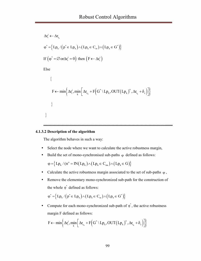
Robust Control Algorithms
99
k
i
t tr r
* * *
k k k se kLp / p Lp Lp C Lp G
If * i
t or r 0 then i
tF r
Else
k k
oi *
t c k k ctk
F min r ,min r F G \ Lp ,OUT Lp , r
………………………………………………………………………………….......
4.1.3.2 Description of the algorithm
The algorithm behaves in such a way:
Select the node where we want to calculate the active robustness margin,
Build the set of mono-synchronised sub-paths φ defined as follows:
o
k k k ms kLp / (n IN Lp Lp C Lp G
Calculate the active robustness margin associated to the set of sub-paths φ ,
Remove the elementary mono-synchronized sub-path for the construction of
the whole *φ defined as follows:
* * *
k k k se kLp / p Lp Lp C Lp G
Compute for each mono-synchronized sub-path of *φ , the active robustness
margin F defined as follows:
k k
oi *
t c k k ctk
F min r ,min r F G \ Lp ,OUT Lp , r

Robust Control Algorithms
100
It should be noticed that in approach 1, the maximal transmissible margin of
the disturbance is determined by kt
r , but in this approach, the margin is fac-
tually increased to k ctr by giving an active control on the transitions of the
parallel concentrated paths.
Stop the algorithm if the following condition is satisfied:
If * i
t or r 0 then i
tF r
4.1.3.3 Analysis of the algorithm
Concerning the algorithm‟s convergence, the behaviour of the second approach
is so similar to the first that a new convergence proof is not useful. The proof of the
formula, which is recursively applied by the algorithm, can be found in(Jerbi et al.,
2009).
The complexity of the computing time is smaller than 6O n , and n is the num-
ber of transitions. The readers interested in a theoretical analysis of the complexity of
the algorithm‟s computing time may consult (Collart-Dutilleul et al., 2013). The algo-
rithm in our work has a modified structure compared with the algorithm in (Collart-
Dutilleul et al., 2013). In our algorithm, each transition is controllable and observable,
which presents a better modeling for the control on the AIVs. The computing time of
algorithm 2 is also acceptable. Although the complexity of algorithm 2 6O n is larg-
er than the first one 4O n , the algorithm 2 indeed increases the robustness margin
for a real industrial topology as shown in the section 4.1.3.4.
4.1.3.4 Illustrative example
To calculate the robustness margin on 22t in Figure 4.6, the compensable margin
and the transmissible margin associated to some mono-synchronized sub-paths are
summarized in Table 4.1. The active similar disturbance control c is generated on
the parallel concentrated paths, which are shown in Table 4.2.
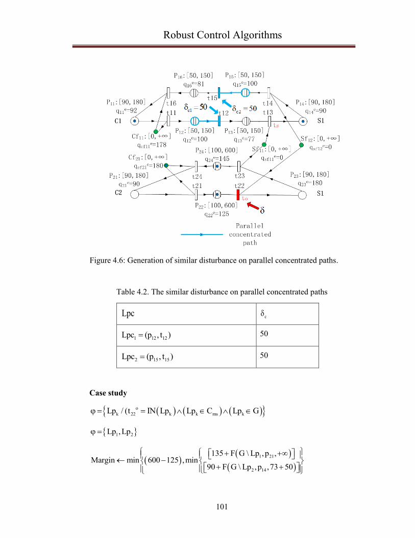
Robust Control Algorithms
101
Figure 4.6: Generation of similar disturbance on parallel concentrated paths.
Table 4.2. The similar disturbance on parallel concentrated paths
Lpc c
1 12 12Lpc (p , t )
50
2 15 15Lpc (p , t )
50
Case study
o
k 22 k k ms kLp / (t IN Lp Lp C Lp G
1 2Lp ,Lp
1 21
2 14
135 F G \ Lp ,p ,Margin min 600 125 ,min
90 F G \ Lp ,p ,73 50

Robust Control Algorithms
102
Step 1: Computation of 1 21F G \ Lp ,p ,
*
3 4Lp ,Lp
1 3 21
1 4 23
min[ ,180 F(G\ Lp \ Lp ,p ,455)]F min
min[ ,25 F(G\ Lp \ Lp ,p , )]
Step 1.1: Computation of 1 3 21F(G\ Lp \ Lp ,p ,455)
* then F 455
Step 1.2: Computation of 1 4 23F(G\ Lp \ Lp ,p , )
* then F
Step 2: Computation of 2 14F G \ Lp ,p ,123
*
5 6Lp ,Lp
2 5 11
2 6 23
min[123,81 F(G\ Lp \ Lp ,p , )]F min
min[123,0 F(G\ Lp \ Lp ,p ,475)]
Step 2.1: Computation of 2 5 11F(G\ Lp \ Lp ,p , )
*
7 8Lp ,Lp
2 5 7 11
2 5 8 14
,180 F(G\ Lp \ Lp \ Lp ,p ,69 50)
,79 F(G\ Lp \ Lp
min[ ]F min
min[ \ Lp , , )]p
Step 2.1.1: Computation of 2 5 7 11F(G\ Lp \ Lp \ Lp ,p ,119)
* then F 119
Step 2.1.2: Computation of 2 5 8 14F(G\ Lp \ Lp \ Lp ,p , )
* then F
Step 2.2: Computation of 2 6 23F(G\ Lp \ Lp ,p ,475)
* then F 475
Algorithm stops

Robust Control Algorithms
103
Margin 213
The active robustness margin on 22t is 213. If any delay disturbance is less than
213 unit time, a false alarm can be avoided, and the system could recover to the initial
normal mode. Using an active robust control generating parallel similar temporal shift,
the robustness margin obtained by the second approach is better than the first ap-
proach.
Let δ=213 be a delay disturbance observed on 22t in Figure 4.6. On the path 1Lp ,
the disturbance can be first partially reduced by 23t to 123=213-(180-90). Then, the
residue of disturbance 123 is reduced by 24t to 78=123-(145-100). As the transmissi-
ble margin of 21cf is , the residue 78 can be totally transmitted to 21p . In other
words, the token in 21cf is also actively delayed with 78 time units. On the path 3Lp ,
the residue 78 is completely decreased to 0 in 21cf , as the compensable margin is 180.
On the path 4Lp , the residue is rejected to 53=78-25. This residue 53 is transmitted
to 23p , and is reduced completely to 0 in 23p . On the path 2Lp , the compensable
margin is 90. So, the disturbance is reduced to 123. This residue can be totally trans-
mitted to 14p , as the transmissible margin of 2Lp is 73 and the parallel similar dis-
turbance is 50. Factually, the token in 13p is also delayed with 123 time units com-
pared to normal firing date of 13t . On the path 5Lp , the residue 123 is rejected to 42
by a compensable margin 81. And, the residue 42 will be decreased completely to 0
on 7Lp and 8Lp , as the compensable margin is 180 and 79 respectively. On the path
6Lp , the residue 123 is transmitted to 23p by 22t . Finally, the residue of disturbance
123 will be surely completely eliminated to 0, because the residue 123 will be re-
duced to 33=123-(213-123) on 22t , if we apply again the approach 2. Finally, the res-
idue 33 is completely eliminated to 0 in 23p .
4.1.4 Comparison between Approach 1 and Approach 2
As discussed in sections 4.1.2.3 and 4.1.3.3, the complexity of computing time
for approach 1 is 4O(n ) , and the complexity of computing time of approach 2 is
6O(n ) . So, concerning the complexity of computing time, approach 1 is better than

Robust Control Algorithms
104
approach 2. A higher order of the complexity in computing time of approach 2 is gen-
erated by the active parallel similar control given on the parallel concentrated paths.
But, concerning the robustness margin on the nodes, the approach 2 is better
than approach 1, Margin1 Margin 2. By the generation of parallel similar temporal
shift, the parallel concentrated paths can transmit more delay robustness because of
k c ctr . In the example shown in Figure 4.6, for a disturbance observed on 22t ,
the robustness margin 213 of approach 2 is better than the robustness margin 163 of
approach 1. But in an extreme condition as shown in Figure 3.1, there is no concen-
trated path in the example, c 0 .In this condition, the value of the robustness mar-
gin on node is computed by applying approach 1, with Margin 1=Margin 2=213.
Figure 4.7: The signal points on the AIV running routes.
The analysis of results implies that approach 2 has a better performance if there
are more controllable transitions on the parallel paths. For example, in Figure 3.1,
there are two transitions between 11p (C1) and 13p (S1) , and, in Figure 4.6, there are
three transitions between 11p (C1) and 14p (S1) . Factually, if the places between C1 and
S1 stand for routes of the AIVs from the QCs to the AYCs, then the transitions can be
seen as the signal points which help the AIV to locate their positions. It is reasonable
that more signal points on the route can increase the location accuracy of the AIVs.
And from a physical view, the signals of the signal points maybe blocked by the mov-
ing cranes, the container stacks or the other AIVs. So more signal points on the routes
can indeed guarantee a better functioning of the AIVs, and increase the safety in the
transit procedures. It is admitted that, the number of the signal points should be given

Robust Control Algorithms
105
basing on the test and analysis result on the container transit filed by the engineers
and the automated vehicle specialists. Because too many signal points will increase
the investment of infrastructure, and will also raise the unnecessary controls on the
AIVs which is strongly related to the management cost.
Figure 4.7.A shows the physical structure of path (t11,p12, t12) of the example
shown in Figure 3.1. And Figure 4.7.B shows the physical structure of the path (t11,
p12, t12, p12, t13) of the example shown in Figure 4.6. The plan B can give a better
control on the AIVs with more signal points on the routes.
So, the transit procedure manager should make a choice to balance the complexi-
ty of computing time, the robustness margin of the system, the infrastructure invest-
ment and the control accuracy. The approach 1 has less complexity in computing time
(4O(n ) ), but less robustness margin and worse control for the AIVs. The approach 2
has more complexity in computing time (6O(n ) ), but larger robustness margin (as
least not less than the approach 1) and better control for the AIVs. If considering the
resilience or the robustness of the system and the safety require for the system, the
approach 2 is might be an even better choice.
4.2 The algorithm based on direct control of tokens’ sojourn time
The section 4.1 presents the approach 1 and approach 2 which are two algo-
rithms to compute the acceptable robustness margin on one node of PTSCEG. The
rejection process of the advance (or delay) disturbance is based on the control of the
transitions (the structure of the PTSCEG) with a delay (respectively an advance) fir-
ing time on the propagation path. The two algorithms guarantee that the rejection is
given as soon as the disturbance is observed. And the approach 2 gives an active par-
allel similar temporal shift as large as possible, but not as soon as the disturbance is
observed because of the constraints about the concentrated paths.
The algorithm presented in this section is based on the direct control of token‟s
sojourn time in a 1-cyclic schedule Gantt graph. This algorithm guarantees the similar
parallel disturbance control is actively given as soon as the disturbance is observed.
This algorithm has also a computing time in polynomial complexity.

Robust Control Algorithms
106
4.2.1 Basic notation
Figure 4.8: The coupling of the tokens presented by Gantt graph.
Definition 4.10: The coupling of tokens is a phenomenon that the tokens from
different elementary circuits enter into one shared place and fuse as one single token
in this shared place.
Let us take the 1-cyclic schedule of tokens in Figure 4.3 as an example. It is pos-
sible to give a 1-cyclic schedule for the tokens as shown in Figure 4.8. This schedule
is shown in Gantt graph. 11v and 12v are two tokens in 1G (C1 S1) ; 21v and 22v
are two tokens in 2
G (C2 S1) ; c1t is one token in the C1 operation space status cir-
cuit; c2t is one token in the C2 operation status circuit; s1t is one token in the S1 oper-
ation space circuit. The coupling of the tokens occurs in the shared places. The s1t and
22v are coupled in 23p , the 21v and c2t are coupled in 21p , and the s1t and 21v are
coupled in 23p etc. For the coupled tokens in the shared places, they fuse into one to-
ken. But when this token exits the shared place, it decomposes again to the initial to-
kens before entering the shared place. From a physical view, an empty AIV 21v enter

Robust Control Algorithms
107
into 21p to take the container, and one free QC ( c2t ) is ready to lift the container from
the vessel and put it on the AIV. The AIV and the crane do the unloading work in 21p .
When the unloading is finished, AIV exits the operation place as a full AIV, and the
crane becomes a free crane again.
Definition 4.11: The coupling point Co is the time point when the coupling of
tokens occurs.
For example, oC 145 is the coupling point of 21v and c2t in 21p .
Figure 4.9: The cutting of the tokens at coupling point.
Definition 4.12:The cutting of token‟s sojourn time on coupling point is to di-
vide the sojourn time of tokens which is not coupled at the coupling point but has
been coupled with the present coupling token before the coupling point.
As shown in Figure 4.9, the token 21v is coupled with c2t at the coupling point
145. Then, the token 21v is coupled with s1t at another coupling point 360. The cou-

Robust Control Algorithms
108
pling point 360 cuts the 21cf into two parts, since c2t has coupled with 21v . Let us
denote the part before (or after) the coupling point as oC B ( oC A respectively). One
part of 21cf has a duration oC B 125 , and the other part has a duration oC A 55 .
Definition 4.13: The disturbance rejection group is a set that only includes all
the disturbed tokens and the tokens coupled by the disturbed tokens.
Definition 4.14: The parallel similar temporal shift group is a set that includes
only the non-disturbed coupled tokens.
Figure 4.10: The classification of the tokens.
The Figure 4.10 shows the coupling progress of the tokens in 1-cyclic schedule
of Figure 4.8. If the disturbance is observed on the sojourn time of 22v in the place
22p , just as the disturbance is observed on 22t in Figure 4.3, the s1t will be coupled
with 22v in the place 23p , then, the token set 1 3Q Q is a disturbance rejection token
group. From the coupling point, the tokens in 1 3Q Q will be given a delay (advance)
control to reject the observed disturbance which is an advance (delay respectively).
The token 11v and c1t are coupled in 11p . Normally, the two tokens finish the staying
in 11p at t 93 . So, when the disturbance is observed at t 90 , it is still possible to
give an active control on the token in 11p , with a parallel similar temporal shift. They

Robust Control Algorithms
109
are in a parallel similar temporal shift group 2Q . The tokens in 2Q will be given a
similar delay (or advance) control if the is a delay (an advance respectively). Dur-
ing the coupling progress, the token groups integrate step by step. 1 3Q Q and 2Q
combine as *Q which is a disturbance rejection token group in 14p . Because after the
coupling point on 14p , all the tokens in *Q should contribute to reduce the delay
(advance) disturbance with advance (delay) control. Progressively, in 11p , *Q and
4Q combine to a new disturbance rejection token group * *
4Q Q Q . And in 23p ,
with oC 360 , a disturbance token group including all the tokens is formed, with
* *
5Q Q Q . During the coupling procedures, the disturbance rejection group ab-
sorbs more and more tokens, and the parallel similar temporal shift groups disappear
gradually.
Definition 4.15: The pure coupling point CoP is a coupling point that the coupled
tokens use the same control strategy (disturbance rejection or parallel similar tem-
poral shift generation) before this coupling point.
Definition 4.16: The mixed coupling point oMC is a coupling point that the cou-
pled tokens use the different control strategies before this coupling point.
As shown in Figure 4.10, oC 1 and oC 145 are the pure coupling points, and
oC 90 , oC 270 , oC 271 and oC 360 are the mixed coupling points where the
tokens from different kinds of tokens groups are coupled.
4.2.1.1 The transmissible margin of the parallel similar temporal shift group
Let us denote
oC the time point where the disturbance is initially observed, all the active con-
trol should be given after this point,
n
oMC the nth mixed coupling point, n N
tQr the transmissible margin of the parallel similar temporal shift group be-
tween the oC and a mixed coupling point n
oMC ,
k
oPC , the kth pure coupling point between oC and n
oMC , k N , max(k) ,

Robust Control Algorithms
110
oCp the operation of tokens cut by the coupling point oC ,
oC B the cutting part of oCp before oC ,
oC A the cutting part of oCp after oC
rQ the disturbance rejection token group,
pQ The parallel similar temporal shift token group
In the parallel similar temporal shift group, it is possible to control the sojourn
time of each token in each place to generate the similar disturbance as the disturbance
observed in rQ . The transmissible margin of the tokens in this group between the oC
and a mixed coupling point n
oMC can be computed using the following formulas
• Case of a delay disturbance in rQ
………………………………………………………………………………….......
For the transmissible margin from oC to n
oMC
If k
oPC ,
il p1o oP
e
tQ ij ijv Q
C C
r min (b q )
(4.11)
il pk k 1ij k ij koP oP C CoP oP
e e k
tQ ij ij ij ij ijv Q
p p p pC C
r min[ (b q ) (b q Rt )]
(4.12)
s.t.
1ij ko oP C
oP
ij kCoP k 1 k
ij k 1 kij k 1oP oP C CC oP oPoP
e
tQ ij ij
p pC Ck
ij e k 1 ep p tQ ij ij ij ij ij
p p pp pC C
max[0, r (b q )],k 1
Rtmax[0, r (b q Rt ) (b q )],k 2
il pnij ijoP oM C CoP oP
e e
tQ ij ij ij ij ijv Q
p p p pC C
r min[ (b q ) (b q Rt )]
(4.13)
As a consequence,

Robust Control Algorithms
111
n 1 k k 1 no oM o oP oP oP oP oM
tQ tQ tQ tQ
kC C C C C C C C
r r r r
(4.14)
……………………………………………………………………………………
If k
oPC
il pno oM
e
tQ ij ijv Q
C C
r min (b q )
(4.15)
…………………………………………………………………………………….
• Case of an advance disturbance in rQ
…………………………………………………………………………………......
For the transmissible margin from oC to n
oMC
If k
oPC ,
il p1ij 1 ij ij 1o oP C C C Co ooP oP
e e 1 e
tQ ij ij o ij ij oP ij ijv Q
p p p p p p pC C
r max [a q ] max[ C A,(a q )] max[ C B,(a q )]
(4.16)
il pk k 1ij k k 1 ij k ij k 1oP oP C C C CoP oP oP oP
e k e k k 1 e
tQ ij ij oP ij ij ij oP ij ijv Q
p p p p p p pC C
r max [a q ] max[ C A,(a q ) Rt ] max[ C B,(a q )]
(4.17)
s.t.
1ij 1 ijo oP C C Co ooP
k 1 kij k 1 k ij k 1oP oP C C CoP oP oP
e e
tQ ij ij o ij ij
p p p p pC Ck
ij e k 1 e k 1
tQ ij ij oP ij ij ij
p p p p pC C
min[0, r (a q ) max( C A,a q )],k 1
Rtmin[0, r (a q ) max( C A,a q Rt )],k 2

Robust Control Algorithms
112
il pnij n ij ij noP oM C C C CoP oM oP oM
e e n e
tQ ij ij oP ij ij ij oM ij ijv Q
p p p p p p pC C
r max [a q ] max[ C A,(a q ) Rt ] max[ C B,(a q )]
(4.18)
As a consequence,
n 1 k k 1 no oM o oP oP oP oP oM
tQ tQ tQ tQ
kC C C C C C C C
r r r r
(4.19)
……………………………………………………………………………………
If k
oPC
il pnij n ij ij no oM C C C Co ooM oM
e e n e
tQ ij ij o ij ij oM ij ijv Q
p p p p p p pC C
r max [a q ] max[ C A,(a q )] max[ C B,(a q )]
(4.20)
……………………………………………………………………………………
4.2.1.2 The compensable margin of the disturbance rejection group
In the disturbance rejection token group, it is possible to control the sojourn
time of each token in each place to reduce the disturbance. The compensable margin
of the tokens in this group between two successive mixed coupling points can be
computed using the following formulas:
Let us denote
cQr the compensable margin the rejection disturbance token group between oC
and 1
oMC , or between n
oMC and n 1
oMC ,
k
oPC , the kth pure coupling point between n
oMC and n 1
oMC , k N , max(k) ,
• Case for a delay disturbance observed on a token
……………………………………………………………………………………...
For the compensable margin from oC to 1
oMC
If k
oPC ,

Robust Control Algorithms
113
il r1ij 1 ij 1o oP C CoP oP
e 1 e
cQ ij ij oP ij ijv Q
p p p pC C
r min [q a ] min[C B,(q a )]
(4.21)
il rk k 1ij k k 1 ij k 1 ij koP oP C C C CoP oP oP oP
e k 1 e k e k
cQ ij ij oP ij ij oP ij ij ijv Q
p p p p p p pC C
r min [q a ] min[C B,(q a )] min[C A,q a Rc ]
(4.22)
s.t.
1ij 1oP oP C
oP
k 1 kij k 1 k ij k 1oP oP C C CoP oP oP
1 e
ij cQ ij ij
p pC C
k e k 1 e k 1
ij cQ ij ij oP ij ij ij
p p p p pC C
Rc max[0, r (q a )],k 1
Rc max 0, r [q a ] min[C A,q a Rc ] ,k 2
il1ij 1 ij 1 ijoP oM C C C CoP oM oM oP
e 1 e e
cQ ij ij oM ij ij oP ij ij ijv Q
p p p p p p pC C
r min [q a ] min[C B,(q a )] min[C A,q a Rc ]
(4.23)
As a consequence,
1 1 k k 1 1o oM o oP oP oP oP oM
cQ cQ cQ cQ
kC C C C C C C C
r r r r
(4.24)
……………………………………………………………………………………
If k
oPC ,
il r1ij 1 ij 1o oM C CoM oM
e 1 e
cQ ij ij oM ij ijv Q
p p p pC C
r min [q a ] min[C B,(q a )]
(4.25)
………………………………………………………………………………….......

Robust Control Algorithms
114
For the compensable margin from n
oMC to n 1
oMC
If k
oPC between n
oMC and n 1
oMC ,
nil p oM
ij n 1 ij 1 ij nC C C CoM oP oP oM
niln 1il r oMoM oP
ij n 1 ij 1C C CoM oP oP
v Q beforeC
e 1 e n e t
ij ij oP ij ij oM ij ij ij
p p p p p p p
cQv
v Q beforeCC C
e 1 e
ij ij oP ij ij
p p p p p
[q a ] min[C B,(q a )] min[C A,q a R ]
r min
[q a ] min[C B,(q a )]
ij nC
oM
n e c
oM ij ij ij
p p
min[C A,q a R ]
(4.26)
s.t.
nij nijoP oM C CC oP oMoP
nij no oM C
oM
e e
tQ ij ij ij ij ij
p p pp pC C
t
ij
e
tQ ij ij
p pC C
max[0, r (b q Rt ) (b q )]
R or
max[0, r (b q )]
nij 1ijoP oM C CC oP oMoP
nijo oM Co
e e
cQ oP ij ij ij ij ij
p p pp pC C
c
ij
e
cQ ij ij
p pC C
max[0, r min(C A,q a R ) (q a )]
R or
max[0, r (q a )]
ilk k 1ij k k 1 ij k 1 ij koP oP C C C CoP oP oP oP
e k 1 e k e k
cQ ij ij oP ij ij oP ij ij ijv
p p p p p p pC C
r min [q a ] min[C B,(q a )] min[C A,q a Rc ]
(4.27)
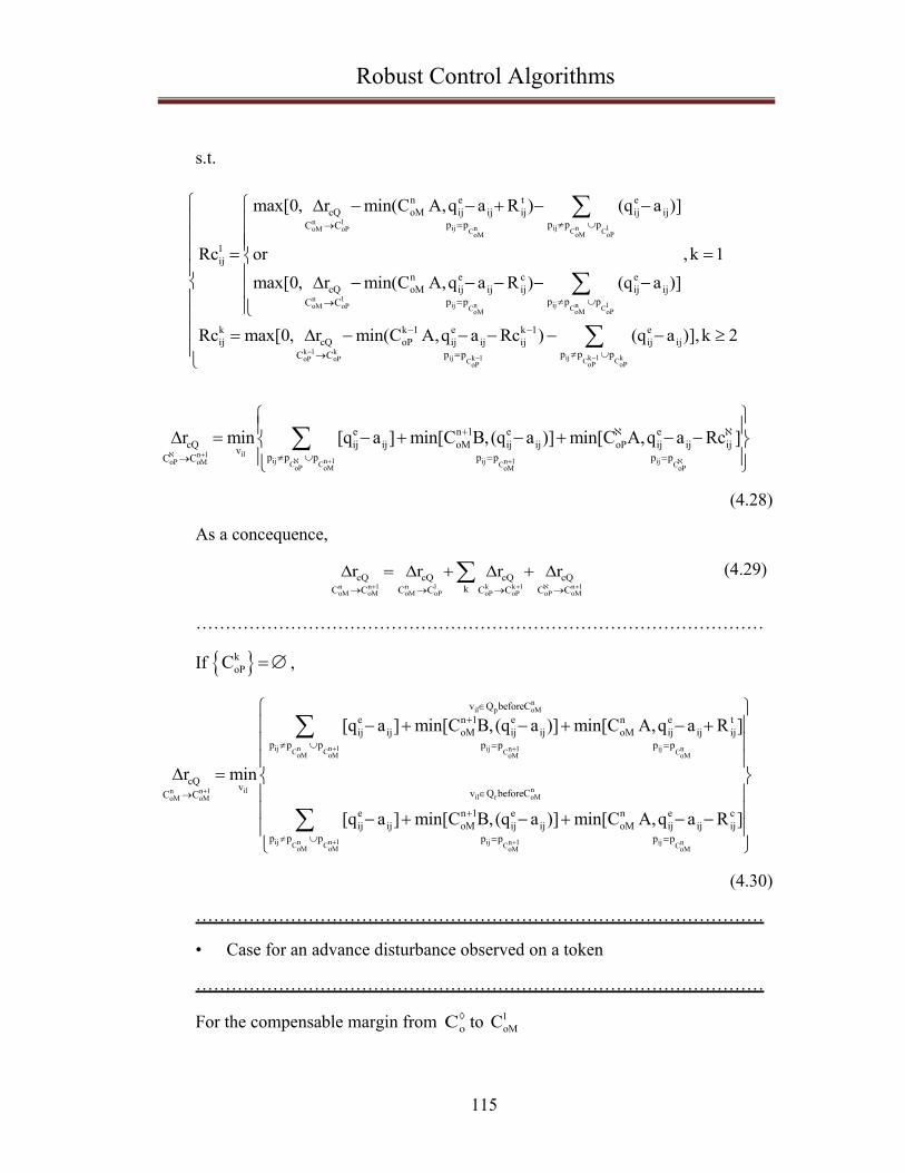
Robust Control Algorithms
115
s.t.
n 1ij n 1ij noM oP C CC oM oPoM
n 1ij n 1ij noM oP C CC oM oPoM
n e t e
cQ oM ij ij ij ij ij
p p pp pC C
1
ij
n e c e
cQ oM ij ij ij ij ij
p p pp pC C
k
ij cQ
C
max[0, r min(C A,q a R ) (q a )]
Rc or ,k 1
max[0, r min(C A,q a R ) (q a )]
Rc max[0, r
k 1 kij k 1 kij k 1oP oP C CC oP oPoP
k 1 e k 1 e
oP ij ij ij ij ij
p p pp pC
min(C A,q a Rc ) (q a )],k 2
iln 1ij n 1 ij n 1 ijoP oM C C C CoP oM oM oP
e n 1 e e
cQ ij ij oM ij ij oP ij ij ijv
p p p p p p pC C
r min [q a ] min[C B,(q a )] min[C A,q a Rc ]
(4.28)
As a concequence,
n n 1 n 1 k k 1 n 1oM oM oM oP oP oP oP oM
cQ cQ cQ cQ
kC C C C C C C C
r r r r
(4.29)
……………………………………………………………………………………
If k
oPC ,
nil p oM
ij n n 1 ij n 1 ij nC C C CoM oM oM oM
niln n 1il r oMoM oM
ij n n 1C CoM oM
v Q beforeC
e n 1 e n e t
ij ij oM ij ij oM ij ij ij
p p p p p p p
cQv
v Q beforeCC C
e n 1 e
ij ij oM ij i
p p p
[q a ] min[C B,(q a )] min[C A,q a R ]
r min
[q a ] min[C B,(q a
ij n 1 ij nC C
oM oM
n e c
j oM ij ij ij
p p p p
)] min[C A,q a R ]
(4.30)
……………………………………………………………………………………
• Case for an advance disturbance observed on a token
……………………………………………………………………………………
For the compensable margin from oC to 1
oMC

Robust Control Algorithms
116
If k
oPC ,
il r1o oP
e
cQ ij ijv Q
C C
r max[ (q b )]
(4.31)
il rk k 1ij k ij koP oP C CoP oP
e e k
cQ ij ij ij ij ijv Q
p p p pC C
r max[ (q b ) (q b Rc )]
(4.32)
s.t.
1ij ko oP C
oP
ij kCoP k 1 k
ij k 1 kij k 1oP oP C CC oP oPoP
e
tQ ij ij
p pC Ck
ij e k 1 ep p tQ ij ij ij ij ij
p p pp pC C
min[0, r (q b )],k 1
Rtmin[0, r (q b Rc ) (q b )],k 2
il r1ij ijoP oM C CoP oP
e e
cQ ij ij ij ij ijv Q
p p p pC C
r max[ (q b ) (q b Rt )]
(4.33)
As a consequence,
1 1 k k 1 1o oM o oP oP oP oP oM
cQ cQ cQ cQ
kC C C C C C C C
r r r r
(4.34)
……………………………………………………………………………………
If k
oPC
il r1o oM
e
cQ ij ijv Q
C C
r max (q b )
(4.35)
………………………………………………………………………………….......
For the compensable margin from n
oMC to n 1
oMC
If k
oPC between n
oMC and n 1
oMC ,

Robust Control Algorithms
117
nil p oM
ij n ij nC CoM oM
niln 1il r oMoM oP
ij n ij nC CoM oM
v Q beforeC
e e t
ij ij ij ij ij
p p p p
cQv
v Q beforeCC C
e e c
ij ij ij ij ij
p p p p
[q b ] [(q b R )]
r max
[q b ] (q b R )
(4.36)
s.t.
nij nijoP oM C CC oP oMoP
nij no oM C
oM
e e
tQ ij ij ij ij ij
p p pp pC C
t
ij
e
tQ ij ij
p pC C
min[0, r (q b Rt ) (q b )]
R or
min[0, r (q b )]
nij 1ijoP oM C CC oP oMoP
nijo oM Co
e e
cQ ij ij ij ij ij
p p pp pC C
c
ij
e
cQ ij ij
p pC C
min[0, r (q b R ) (q b )]
R or
min[0, r (q b )]
ilk k 1ij k ij koP oP C CoP oP
e e k
cQ ij ij ij ij ijv
p p p pC C
r max[ (q b ) (q b Rc )]
(4.37)
s.t.
n 1ij n 1ij noM oP C CC oM oPoM
n 1ij n 1ij noM oP C CC oM oPoM
k 1 koP oP
e t e
cQ ij ij ij ij ij
p p pp pC C
1
ij
e c e
cQ ij ij ij ij ij
p p pp pC C
k e
ij cQ ij
C C
min[0, r (q b R ) (q b )]
Rc or ,k 1
min[0, r (q b R ) (q b )]
Rc min[0, r (q b
ij k 1 kij k 1 C CC oP oPoP
k 1 e
ij ij ij ij
p p pp p
Rc ) (q b )],k 2

Robust Control Algorithms
118
iln 1ij ijoP oM C CoP oP
e e
cQ ij ij ij ij ijv
p p p pC C
r max[ (q b ) (q b R )]
(4.38)
As a consequence,
n n 1 n 1 k k 1 n 1oM oM oM oP oP oP oP oM
cQ cQ cQ cQ
kC C C C C C C C
r r r r
(4.39)
……………………………………………………………………………………
If k
oPC ,
nil p oM
ij n ij nC CoM oM
niln n 1il r oMoM oM
ij n ij nC CoM oM
v Q beforeC
e e t
ij ij ij ij ij
p p p p
cQv
v Q beforeCC C
e e c
ij ij ij ij ij
p p p p
[q b ] [(q b R )]
r max
[q b ] (q b R )
(4.40)
……………………………………………………………………………………
4.2.2 Approach 3: Generation of the parallel similar disturbance as soon as the dis-
turbed is observed
This approach generates a similar temporal shift in the parallel token group as
soon as the disturbance is observed in order to avoid the death of tokens on the cou-
pling points. Therefore, constraints violations are avoided. If the disturbance is a de-
lay (an advance), then the temporal shift will be a delay (respectively an advance) ob-
tained by changing the sojourn time of tokens belonging to the parallel similar tem-
poral shift group. The approach 2 can‟t guarantee the similar temporal shift is given
as soon as the disturbance is observed, but the approach 3 can.
Surely, for the tokens in the disturbance rejection group, the rejection control is
also given as soon as the disturbance is observed.
Factually, the approach 3 applies two strategies, the rejection of the disturbance
in the disturbance rejection group and the generation of the similar temporal shift in
the parallel similar temporal shift group. The approach 3 allows:

Robust Control Algorithms
119
• To reduce the disturbance by compensable control on the tokens in disturb-
ance rejection group as soon as the disturbance is observed,
• To generate the parallel similar temporal shift on the tokens in the parallel
similar temporal shift group as soon as the disturbance is observed.
The computation of the compensable control margin and the parallel similar
temporal shift margin can be referred to the formulas in the sections 4.2.1.1 and
4.2.1.2.
4.2.2.1 Algorithm
This is also a recursive algorithm allowing the active rejection of the disturbance
as soon as it is observed, while considering an active generation of the parallel similar
temporal shift as soon as the disturbance is observed. The number of tokens in the
disturbance rejection group increases during the computation progress, conversely,
the number of the parallel similar temporal shift groups decreases.
Let us denote
AQ the set including all the tokens,
rQ the disturbance rejection group,
oC the time point where the disturbance is initially observed, all the active con-
trol should be given after this point,
n
oMC the nth mixed coupling point, n N ,
n
pQ the parallel similar temporal shift group having a n
oMC with rQ ,
0t the local robust margin of the sojourn time of the initially disturbed token in
the place ijp , for a delay (an advance) disturbance e
0 ij ijt b q ( e
0 ij ijt a q respec-
tively),
tQr the transmissable margin of the parallel similar temporal shift group be-
tween the oC and a mixed coupling point n
oMC ,
cQr the compensable margin the rejection disturbance token group between oC
and 1
oMC , or between n
oMC and n 1
oMC .

Robust Control Algorithms
120
The following algorithm is for the computing a delay disturbance margin. How-
ever, the structure of the algorithm for an advance robustness margin is almost the
same, which is not discussed in this thesis.
……………………………………………………………………………………...
Initialize
rQ is the set including only the tokens disturbed initially at oC ,
and n=1
……………………………………………………………………………………
np
1o oM
n
0 cQ r oM tQC C
Margin min[ , F , , ]t r Q C r
np
n
r oM tQF , ,Q C r
{
n
r r pQ Q Q ,
n=n+1,
If ( r AQ Q or n 1ptQ
r =0) then n 1ptQ
F r ,
Else
{
n 1 np p
n 1 noM oM
n
cQ r oMtQ tQC C
F min[ r , r Q CF , ], r
}

Robust Control Algorithms
121
}
………………………………………………………………………………….......
4.2.2.2 Description of the algorithm
The algorithm behaves in such a way:
• Select the place where we want to calculate the robustness margin of the so-
journ time of the token in this place,
• Build the sets of the initial disturbance rejection group rQ and the parallel
similar temporal shift group n
pQ ,
• Calculate the compensable robustness margin of the initial disturbance re-
jection group rcQr , and the transmissible robustness margin of n
ptQr ,
• Add the set n
pQ to the set rQ , defined as:
n
r r pQ Q Q
• Compute the robustness margin with a recursive function:
n=n+1
n 1 np p
n 1 noM oM
n
cQ r oMtQ tQC C
F min[ r , r Q CF , ], r
• Stop the algorithm if the following condition is satisfied:
If ( r AQ Q or n 1ptQ
r =0) then n 1ptQ
F r .
4.2.2.3 Analysis of the algorithm
The above algorithm applies the robustness formulas on all the tokens. The algo-
rithm is based on function F, which is called recursively using a part of the tokens un-
til all the tokens are used by F or one transmissible margin is 0.
The convergence of the algorithm can be proved as follows.
• Since the space status circuit has just one token, this token can couple all the
tokens in the process circuits which share the space status circuit in a finite

Robust Control Algorithms
122
number of cycle time iW C . iW is the number of tokens in process circuit
iG . Since all the space status circuits have just one token, the tokens in the
process circuits can couple every other token in a finite number of cycle
time imax(W ) C . So, all the tokens can be coupled in a finite number of
cycle time imax(W ) C .
• Since all the tokens are coupled in imax(W ) C , then, there are a finite
number of the coupling points oC (including the pure coupling points and
the mixed coupling points) in this finite number of cycle time. So, the num-
ber of the mixed coupling points is also finite in this finite number of cycle
time.
• So, F uses a limited number of mixed coupling points oMC recursively until
all the tokens are used ( r AQ Q ) or n 1ptQ
r =0. And the algorithm stops if
r AQ Q or n 1ptQ
r =0. Then, the convergence of the considered algorithm is
proved.
The polynomial computation time of this algorithm can be proved as follows.
• Let us denote the number of all the places in PTSCEG as pN . Considering
the repetition of 1-cyclic schedule, these pN places appear in a cycle time
in the Gantt graph. Then, in imax(W ) C , there are at most p iN max(W )
places. So, there are at most p iN max(W ) coupling points which are the be-
ginning point of the shared places.
• For each coupling point, it should compare among the robustness margins of
at most iW tokens (all the tokens). For each token, on considering at
most p iN max(W ) cutting operations on the sojourn time of tokens, there
are at most p i2N max(W ) operations (divided by the cutting or not) which
are used to compute the transmissible margin or the compensable margin. In
total, for computing all the robustness margin of the all disturbance rejection
groups or the parallel similar temporal shift groups, the number of the com-

Robust Control Algorithms
123
puting operation is p i i p iN max(W ) W 2N max(W ) . The complexity of
the computing time is 5O(n ) .
• There are at most iW mixed coupling points which should be less than
the number of all the tokens. Given all the transmissible margin of all the
parallel similar temporal shift groups and all the compensable margin of all
the disturbance rejection groups, the number of the calculation steps of F to
compute the robustness margin of a token in a place is less than iW . So
the global complexity of computing time for the algorithm of approach 3 is
at most 7O(n ) .
The above analysis uses some rough approximations which aim to show that the
computing time is reasonable. For approach 1 and approach 2, the complexity of
computing time of algorithms depend on the number of the transitions, but the algo-
rithm of approach 3 depends on the number of the places in PTSCEG and the number
of all the tokens.
4.2.2.4 Illustrative example
Figure 4.11: The transmissible margin and compensable margin for token groups.

Robust Control Algorithms
124
To calculate the robustness margin on 22t of PTSCEG in Figure 4.3, it can also
be seen as to calculate the robustness margin of the sojourn time of the token 22v in
the place 22p in Figure 4.8.
The Figure 4.11 shows the classification of the tokens, the transmissible margins
of the parallel similar temporal shift groups and the compensable margins of the dis-
turbance rejection groups. We apply the algorithm of approach 3 to compute the ro-
bustness margin of the token 22v which has a delay disturbance observed in the place
22p .
Case study
……………………………………………………………………………………...
Initialize
r 1Q Q
n=1
……………………………………………………………………………………
1p
1
r oM tQ475 0 Q CMargin min[ , , ]rF ,
Step 1: Computation of 1p
1
r oM tQF , ,Q C r
r r 3Q Q Q
n=1+1
1 2 2p p p
1 2oM oM
2 2
cQ r oM r oMtQ tQ tQC C
F , ,F min[ r , r Q C r ] min[ ,90 Q ]F r, ,C
Step 1.1: Computation of 2p
2
r oM tQF , ,Q C r
r r 2Q Q Q
n=2+1

Robust Control Algorithms
125
2 3 3p p p
2 3oM oM
3 3
cQ r oM r oMtQ tQ tQC C
F , ,F min[ r , r Q C r ] min[211,0 Q CF , r ],
Step 1.1.1: Computation of 3p
3
r oM tQF , ,Q C r
r r 4Q Q Q
n=3+1
3 4p p
3 4oM oM
4
cQ r oMtQ tQC C
F min[ r , r ,Q CF r, ]
4p
4
r oM tQmin[119,0 Q C , r ]F ,
Step 1.1.1.1: Computation of 4p
4
r oM tQF , ,Q C r
r r 4Q Q Q
n=4+1
r AQ Q
F (455 565) 1020
Algorithm stops
Margin 209
The active robustness margin of sojourn time of 22v in 22p is 209. If any delay
disturbance is less than 209, a false alarm can be avoided. The system can recover to
the initial 1-cyclic schedule without death of the tokens at the level of coupling points,
if giving an active robust control.
Let 209 be a delay disturbance observed on 22v in 22p in Figure 4.11. Fac-
tually, between 14p and 23p in S1 space status circuit, there is a free status place 12sf
with a transmissible margin. So, the delay can be transmitted to the place 23p by
1
oMC . Then, from the first mixed coupling point to the second, the disturbance is re-
duced to 119 with 1 2oM oM
cQ
C C
r 90
. The transmissible margin of token group 2Q is

Robust Control Algorithms
126
211>119. So, the residue of the disturbance 119 can be transmitted to 14p by 2
oMC .
There is no disturbance rejection between the second and third mixed coupling points,
because the compensable margin is 0. The transmissible margin of 4Q is 119. The
residue 119 can be transmitted to 11p by 3
oMC . There is also no rejection of disturb-
ance between 3
oMC and 4
oMC because of 3 4oM oM
cQ
C C
r 0
. But the residue 119 can be
transmitted to 23p passing 4
oMC , because the transmissible margin of 5Q is
4o oM
cQ
C C
r min(455, ) 565 1020
. After the mixed coupling point 4
oMC , all the to-
kens in the system can run in the initial 1-cyclic schedule without any token death.
All the tokens are still delayed with the same disturbance 119. In other words, the 1-
cyclic schedule is delayed for 119 unit time overall. The residue 119 can always be
neglected considering the infinite repetition of 1-cyclic schedule. However, the resi-
due may be rejected to 0 if the compensable margin between the pure coupling points
for all the tokens in AQ is computed. In a cycle time, the total compensable margin is
k k 1oP oP
cQ
k C C
r 0
. In a finite number of cycles, the residue is reduced to 0, if
k k 1oP oP
cQ
k C C
r 0
.
4.2.3 Comparisons with Approach 1 and Approach 2
Concerning the robustness margin, let us take the robustness margin of token
22v in 22p as samples to make the comparisons,
• Let us denote example in Figure 4.3 as E1 which has concentrated paths in
the process circuits. The result of the illustrative example in section 4.2.2.4
shows the robust margin of approach 3(Margin 3=209) is better than ap-
proach 1(Margin 1=163), but worse than approach 2(Margin 2=213).
• Let us denote example in Figure 3.1 as E2 which has no concentrated paths
in the process circuits. For this example, the 1-cyclic schedule can be given
in Figure 4.12. Applying the three approaches on E2, Margin 3=209 and
Margin 1=Margin 2=213, the approach 3 is worse than the other two ap-
proaches.
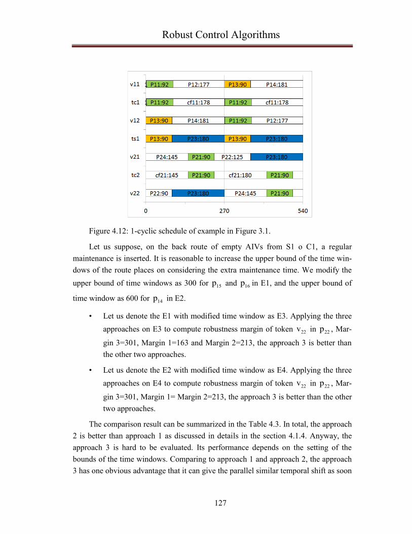
Robust Control Algorithms
127
Figure 4.12: 1-cyclic schedule of example in Figure 3.1.
Let us suppose, on the back route of empty AIVs from S1 o C1, a regular
maintenance is inserted. It is reasonable to increase the upper bound of the time win-
dows of the route places on considering the extra maintenance time. We modify the
upper bound of time windows as 300 for 15p and 16p in E1, and the upper bound of
time window as 600 for 14p in E2.
• Let us denote the E1 with modified time window as E3. Applying the three
approaches on E3 to compute robustness margin of token 22v in 22p , Mar-
gin 3=301, Margin 1=163 and Margin 2=213, the approach 3 is better than
the other two approaches.
• Let us denote the E2 with modified time window as E4. Applying the three
approaches on E4 to compute robustness margin of token 22v in 22p , Mar-
gin 3=301, Margin 1= Margin 2=213, the approach 3 is better than the other
two approaches.
The comparison result can be summarized in the Table 4.3. In total, the approach
2 is better than approach 1 as discussed in details in the section 4.1.4. Anyway, the
approach 3 is hard to be evaluated. Its performance depends on the setting of the
bounds of the time windows. Comparing to approach 1 and approach 2, the approach
3 has one obvious advantage that it can give the parallel similar temporal shift as soon

Robust Control Algorithms
128
as the disturbance is observed. This advantage increases the transmissible margins.
The other two approaches can‟t guarantee the parallel similar control is given just af-
ter the appearance of the disturbance. However, the approach 3 has also a disad-
vantage. During the coupling progress, the tokens are tied up to a unique set gradually.
The liberty to change the sojourn time of the tokens is somehow restricted, which
causes the decrease of transmissible margin or compensable margin sometimes. Thus,
the advantage increasing the robust margin and the disadvantage decreasing the ro-
bust margin make the performance of approach 3 strongly depend on the setting of
example‟s time windows.
Table 4.3: The robustness margins of 3 approaches
Examples Margin 1 Margin 2 Margin 3
E1 163 213 209
E2 213 213 209
E3 163 213 301
E4 213 213 301
Concerning the complexity of computing time, the approach 1 is about 4O(n ) ,
approach 2 is less than6O(n ) and approach 3 is less than
7O(n ) . It should be no-
ticed that, for approach 1 and approach 2, n stands for the number of transitions, but
for approach 3, n stands for the number of tokens and places. All of these 3 ap-
proaches can give a robustness margin on a node in PTSCEG in polynomial time. If
the system is not very complex, the computing time should be acceptable from real
industrial application viewpoint, such as the medium-sized seaport container transit
procedures studied in our work. As shown in Figure 2.10, the number of transitions,
the number of places and the number of tokens are accountable, so the three algo-
rithms are reasonably applicable.
Concerning the complexity of control on all the tokens to deal with the disturb-
ance, the approach 1 and the approach 2 focus on the control the firing time of the
transitions. By these two approaches, it is possible to evaluate the influence of the
disturbance for all the tokens in system by the semantic definition of PTSCEG, but it

Robust Control Algorithms
129
is not obviously shown in the relative algorithms. However, the approach 3 has a
Gantt graph structure base, and all the tokens are taken into account to compute the
robustness margin. Comparing the approach 1 and approach 2, the approach 3 makes
it easier to evaluate of the disturbance‟s influence on the whole system. On the man-
agement level in real industrial processes such as the control on the AIVs, it is inter-
esting to know directly the influence of disturbance for each AIV or cranes. From
the viewpoint of container transit manager, the approach 3 may be more attractive
than the other two approaches
4.3 Conclusion
In this chapter, we present three approaches to compute the robustness margin
on a node of container transit system. Concretely, approach 1 and approach 2 are
based on modifying the algorithms in (Collart-Dutilleul et al., 2013, Mhalla et al.,
2013b). These two modified algorithms are more suitable to the container transporta-
tion procedures. In addition, the modified algorithm includes a new sophisticated def-
inition of active control on concentrated parallel path which avoids the extra disturb-
ances caused by the active parallel control (see in Definition 4.9). The algorithm 3 is
totally a new contribution. Theoretically, these methods can be applied to any manu-
facturing systems modeled by PTSCEG which are not very complex. If the disturb-
ance of AIVs or cranes is located in the robustness margin, it is can be reduced by ac-
tive control on changing the firing time of transitions (the passing time of signal
points) or changing the sojourn time of tokens (the staying time of AIVs). And the
container transit procedure can recover to its initial 1-cyclic schedule mode without
rescheduling.
Three robustness margin algorithms are convergent and have polynomial com-
puting time. For a system not very complex, such as the container transit procedures
in a medium sized seaport, the number of the nodes, the number of the tokens and the
number of the places are not so large. So, the computing time for the robustness mar-
gin on the nodes of system is acceptable. Before the arrival of the vessels, it is possi-
ble to give a cyclic schedule with known robustness margin of each node on the de-
signed routing plan. So, the robust cyclic scheduling can be seen as a predictable
scheduling. When the container transit task begins, the cyclic schedule is used. If a
disturbance is located in the robustness margin, we reduce it by robustness algorithms.
If not, we may reschedule the task by MIP in just a few seconds. Thus, the robust cy-

Robust Control Algorithms
130
clic scheduling can be also seen as a reactive scheduling dealing with the disturbance
in real time.
However, the three algorithms have their own properties individually. The com-
plexity of computing time for approach 1, approach 2 and approach 3 are 4O(n ) ,
6O(n ) and 7O(n ) respectively. The approach 2 is better than approach 1 at the level
of robustness margin because of a parallel similar temporal control on the parallel
concentrated paths. For the container transit procedure, if more signal points are set
on the route to help locate the position of AIVs, the approach 2 has better perfor-
mance than approach 1. More signal source points imply more accuracy to locate the
position of AIVs, which improve the safety management of the system. The approach
3 can give the parallel similar temporal control when the disturbance is observed,
which increase the transmissible margins. But the approach 3 loses liberties of chang-
ing the sojourn time of the tokens during the coupling progress, which decreases the
transmissible margins or the compensable margins. The robustness margin of ap-
proach 3 is not determined to be better than the other two approaches. The robustness
margin of approach 3 depends on the setting of time windows of system. But the ap-
proach 3 can directly give an evaluation of the influence of the disturbance for all the
tokens (the AIVs in the container transit example) in system, which maybe more in-
teresting to the manager of real industrial processes.

Conclusions and Perspectives
131
Chapter 5 Conclusions and Perspectives
Conclusions
In this thesis, we present a robust control 1-cyclic scheduling methodology for
the container transit procedures in a medium sized seaport. This methodology is
proved to be applicable, practical and efficient in the robust supervision and man-
agement of automated intelligent transport system in the small and medium sized con-
tainer terminals.
Figure 5.1: The structure and procedures of robust cyclic methodology.
With the known information about the container transit task, the PTSCEG mod-
elling and the MIP modelling can give the cyclic schedule in short time before the

Conclusions and Perspectives
132
arrival of vessels. At the same time, the robustness margins of this cyclic schedule
can be quickly computed by using the robustness algorithms. When the stevedoring
begins, the containers are transported by the AIVs with the given cyclic schedule. If a
delay or an advance disturbance is observed in the transit procedure, we compare this
observed disturbance with the given robustness margin. If the disturbance is located
in robustness margin, we use the robustness algorithms to reduce or eliminate the dis-
turbance in a few cycle times. If the disturbance is out of the robustness margin, we
use the MIP modelling technique to compute a new cyclic schedule in short time.
Thus, our robust cyclic scheduling methodology is not just a predictable scheduling,
but can be also seen as a reactive scheduling in real time. Our work content and the
procedures of robust cyclic scheduling methodology are shown in Figure 5.1.
Our work makes some contributions both for academic research and for the real
industrial application.
From the academic view, first, the container transit procedure in a medium sized
seaport is modelled by PTSCEG which is always used in the job-shop problem mod-
elling before our work. Second, 1-cyclic scheduling problem with time windows and
transport resource (AIV) in a medium sized seaport is solved by MIP technique in a
short time. Before our work, the MIP is usually seen in the cyclic job-shop scheduling
problem. In these job-shop problems, the transport resources are always neglected.
The third, the robust algorithms used for manufacturing problems in (Collart-
Dutilleul et al., 2007, Mhalla et al., 2013b) are modified to be better suitable for the
robust control on AIVs in container transit procedures. The fourth, a new algorithm
having a structure base in Gantt graph is proposed. Using the new algorithm, it is
much easier to evaluate the influence of the disturbance for each token in system. To-
tally speaking, we do offer some references to the researcher who wants to extend the
utilities of PTSCEG, MIP modelling and robust cyclic scheduling in different indus-
trial area. Moreover, we give new ideas about how to study the robust control of to-
kens in schedule presented by Gantt graph.
From the real industrial view, considering the background of our work, the In-
TraDE project, first we optimize the traffic flow within the confined spaces of small
and medium sized ports with overall optimal cycle time (the reciprocal of productivi-
ty). Second, we use as few AIVs as we can finish the container transit task, which
improves the clean production in container terminal with less energy cost. The third,

Conclusions and Perspectives
133
we develop new algorithms for robust supervision of automatic intelligent transporta-
tion system to reduce or eliminate the disturbances. The fourth, we propose a new and
complete methodology which can improve the efficiency whilst ensuring safety. We
are not sure the cyclic scheduling is strictly better than the other scheduling methods
in an idealized environment without disturbance, but the robust cyclic scheduling may
lead a better performance of the overall productivity on taking the unpredictable and
inevitable perturbations into account for a complex seaport environment.
Perspectives
In the future, we propose the following interesting directions raised by this thesis:
• In the section 2.4.4, we present the intersection modelling using PTSCEG.
Factually, the intersections of the AIVs‟ routes can be seen as the crossroads
in cities or towns. It is possible to extend this intersection modelling to study
the control of the traffic lights of crossroads. And the transport network can
be seen as the intersections plus the routes among intersections. It is possible
to use the PTSCEG modelling techniques to model and to study the intelli-
gent control of the traffic in smart cities or districts.
• The 1-cyclic scheduling method presented in Chapter 3 can be applied to
more examples to verify its efficiency for systems are more complex.
• In Chapter 3 and Chapter 4 , comparing to the almost infinite repetitions of
1-cyclic schedule in steady state, we neglect the transient period of two 1-
cyclic schedules which is presented in (Calvez et al., 1998, Bourdeaud'huy
et al., 2011). But, it is still interesting to study the robust control algorithm
which can also be applied in the transient period of cyclic schedules.
• The algorithm of approach 3 can insert the parallel similar temporal shift as
soon as the disturbance is observed, which can increase the transmissible
margins. But the coupling of tokens limits the changing of tokens‟ sojourn
time, which decreases the compensable margins and transmissible margins.
It is interesting to make a modification of algorithm 3 to weaken the influ-
ence of the coupling operation while the modified one can still insert the
parallel active control as soon as the disturbance is observed. It is possible to

Conclusions and Perspectives
134
have a modified algorithm 3 which is absolutely better than algorithm 2 on
the level of robustness margin.
• The robust control approach 3 is a recursive convergent strategy with com-
puting operation on the coupling points of shared places in the Gantt graph,
which is not like the approach 1 and approach 2 based on the PTSCEG. The
approach 3 can be applied on a cyclic schedule, but non-cyclic schedule too.
The structure base of approach 3 is Gantt graph. For the non-cyclic schedule
presented by Gantt graph, it also has the shared places with coupling points
if shared machines or other shared resources are used in this schedule. If it is
possible to make the products of non-cyclic schedule coupled in a finite time.
Then, it is possible to extend the algorithm of approach 3 to non-cyclic
schedule robust control.
• The robustness algorithms have just been applied on manufacturing system
in (Collart-Dutilleul et al., 2007, Collart-Dutilleul et al., 2013, Mhalla et al.,
2013a, Mhalla et al., 2013b) and on the container transit system in this thesis.
Considering the polynomial complexity for computing time, it is possible to
apply the algorithms in the robust control of intelligent traffic management
in smart cities, the supply chains, the aircraft scheduling in airports etc.
which always face the time disturbance from inner or outer environment
maybe causing a violation in the confined shared spaces.
• There are still a lot of works for realizing the real automated intelligent
transportation in container terminals, such as the protocol conformance of
intelligent devices, the coordination and conflict of man-driven vehicles and
AIVs in the operations space, the implementation of our methodology into
the real control system of AIVs, etc.

135
Appendices
The new model (call it NMW) for work in progress (WIP) minimization in
(Zhang et al., 2014) has only 4 constraint families, on considering 7 families in model
(Bourdeaud'Huy and Korbaa, 2006) (call this model MBK); The models (call it NMC)
for cycle time minimization in this paper (Zhang et al., 2014) has only 5 constraint
families, on considering 8 constraint families in model in (Ben Amar et al., 2011)
(call this model MAR). The models in the paper (Zhang et al., 2014) shorten obvious-
ly the computing time as shown in Table 1 and Table 2.
Table 1. Computing time for WIP minimization
Model Processing time (s)
NMW 0.07 0.12 0.06 0.09 0.10 0.04 0.10 0.07 0.07 0.07 0.079
MBK 0.15 0.20 0.21 0.24 0.17 0.15 0.15 0.17 0.15 0.24 0.183
Table 2. Computing time for cycle time minimization
Model Processing time (s)
NMC 0.07 0.12 0.10 0.12 0.12 0.12 0.10 0.09 0.12 0.10 0.106
MAR 0.14 0.15 0.14 0.17 0.15 0.12 0.12 0.17 0.20 0.17 0.153
The gain for computing time can be calculated by the following formulation (Ben Amar
et al., 2007).
(
)
Gain for Table 1:
(
)
Gain for Table 2:
(
)

136
The 1-cyclic schedules for WIP minimization found by NMW and MBK are
shown in the following figures.
Fig.1.a. Schedule achieved by NMW Fig.1.b. Schedule achieved by MBK
The 1-cyclic schedules for minimizing cycle time found by NMC and MAR are
shown in the following figures.
Fig.2.a. Schedule achieved by NMC Fig.2.b. Schedule achieved by MAR
The readers interested in the description of the problem and the details about the
MIP constraints may consult in (Zhang et al., 2014).

137
Glossary
• G : the PTSCEG model
• iG : ith elementary circuit represents the process circuit or the space status
circuit, i N
• ijp : jth place of iG , the places stand for the operation space of QCs, AYCs,
the intersections, the paths, and the free status of a shared space j N
• ijt : jth transition of iG
• o o
ij ijp (p ) : the input (output) transition of ijp
• ilV : the l th token for iG , Nl
• ijs : entering date of one token in ijp , ijs 0
• ijq : the sojourn time of one token in ijp , ijp 0
• e
ijq : the expected sojourn time of tokens to realize the demanded cycle time
of system, e
ijq 0
• ija : the lower bound of ijq , ija 0
• ijb : the upper bound of ijq , ijb 0
• W : total number of tokens in G , W N
• iW : the number of tokens in iG , iW N
• limitW : the limit number of tokens in G ,
limitW N
• limit
iW : the limit number of tokens in iG , limit
iW N
• C : variable stands for cycle time of G , C 0
• iC : variable stands for cycle time of circuit iG , iC 0

138
• minC : the minimal cycle time of G ,
minC 0
• maxC : the maximal cycle time ofG ,
maxC 0
• I : I max i , the number of iG
• iJ : number of places for iG
• ij : Boolean variable
• ' 'i j
ij : Boolean variable
• msC the set of mono-synchronised sub-paths,
• seC the set of elementary mono-synchronised sub-paths,
• n the transition node where the disturbance is observed,
• maxn the local active robustness of the node n,
• F the recursive function in algorithm,
• i
tr the value of kt
r when F was used the ith time.
• c delays generated on the controlled transition firings on the concentrated
parallel path
• oC the time point where the disturbance is initially observed, all the active
control should be given after this point,
• n
oMC the nth mixed coupling point, n N
• tQr the transmissable margin of the parallel similar temporal shift group
between the oC and a mixed coupling point n
oMC ,
• cQr the compensable margin the rejection disturbance token group between
oC and 1
oMC , or between n
oMC and n 1
oMC ,

139
• k
oPC the kth pure coupling point between oC and n
oMC , k N ,
max(k) ,
• oCp the operation of tokens cut by the coupling point oC ,
• oC B the cutting part of oCp before oC
,
• oC A the cutting part of oCp after
oC
• rQ the disturbance rejection token group,
• pQ The parallel similar disturbance token group

140

141
Résumé étendu en Français
Introduction
La contribution principale dans ce travail de thèse concerne la méthodologie de
planification cyclique robuste appliquée aux systèmes de transport de conteneurs à
l‟aide de véhicule intelligent automatisée (AIV) dans les ports de taille moyenne.
Nous avons effectué ce travail dans le cadre du projet Européen nommé „InTraDE‟
(Intelligent Transportation for Dynamic Environment, 2009-2013)
Figure 1 : Structure et méthodologie cyclique robuste.
La méthode de planification cyclique robuste que nous utilisons fonctionne de la
manière suivante : l'emplacement des conteneurs sur les bateaux et sur les piles de
triage peut être connu à l‟avance, au moins quelques heures avant l‟arrivée des
navires à quai dans un port de taille moyenne. Comme le montre la figure 1. Sachant

142
que les informations concernant les tâches de transit de conteneurs sont connues, les
graphes d‟évènement P-temporels fortement connexes (PTSCEG) et la
programmation mixte en nombres entiers (MIP) sont utilisées afin de trouver un
ordonnancement cyclique „optimale‟ dans un temps relativement court et ceci avant
l‟arrivée des navires à quai. Dans le même temps, l’algorithme de robustesse sera
utilisé pour calculer rapidement les marges de robustesse pour cet ordonnancement
cyclique. Lorsque la manutention commence, les conteneurs sont transportés par les
AIV conformément à l‟ordonnancement cyclique proposé. Si une perturbation (retard
ou avance) est observée dans la procédure de transit, nous comparons cette
perturbation observée avec la marge de robustesse calculée précédemment. Dans le
cas où elle est située dans la marge de robustesse, elle pourra être réduite ou éliminée
en quelques cycles grâce à l‟algorithme de robustesse. Par contre, si elle est en dehors
de la marge de robustesse, nous utilisant dans ce cas, la MIP pour trouver un nouvel
ordonnancement cyclique en un temps relativement court. Ainsi, la méthodologie
d‟ordonnancement cyclique robuste que nous proposons et non seulement un
ordonnancement prédictive mais également une méthodologie d‟ordonnancement
réactive en temps réel.
Cette thèse est composée de cinq chapitres organisés de la manière suivante:
Dans le chapitre 1, nous exposons un état de l‟art et une étude bibliographique
mettant l‟accent sur trois aspects
La pertinence de l‟application d‟une supervision et un management robuste
pour le transport automatisé et intelligent dans les ports de taille moyenne,
Les possibilités ainsi que les avantages à l‟application d‟un ordonnancement
cyclique pour le contrôle robuste,
Les raisons des différents choix de méthodes ou outils mathématiques comme
PTSCEG, MIP et algorithmes de robustnesse.
Le chapitre 2 se focalise sur la modélisation du système en utilisant les graphes
d‟évènement P-temporels fortement connexes (PTSCEG).
Dans le chapitre 3 nous traitons en se basons sur la description donné par
PTSCEG, une modélisation mathématique nommée MIP du système qui permet de
calculer les temps de séjours des tâches dans les fenêtres de temps. L‟utilisation du

143
CEPEX, permet de trouver un ordonnancement 1-cyclique „optimal‟ en un temps
réduit.
Le chapitre 4 détaille la combinaison de commande robuste et ordonnancement
cyclique. Trois algorithmes sont proposés. Tous ces algorithmes ont un temps de
calcul polynomial.
Le chapitre 5 conclut les contributions et les originalités de cette thèse. Des
perspectives intéressantes pour la poursuite des travaux sont également proposées.
Chapitre 1 Etat de l’art
Partant du fait que la gestion des conteneurs dans les ports maritimes de taille
moyenne est en constante évolution, en effet, la variation des conditions des
terminaux, la visibilité réduite sur des évènements futurs ne permet pas de proposer
une planification précise des tâches à accomplir. Une surveillance accrue des
systèmes de transport intelligent automatisée utilisée dans ces espaces de
fonctionnement confinés est demandée afin d‟éliminer toute perturbation. Les
opérations de chargement/déchargement ou de transit peuvent être considérées
comme des opérations répétitives, de ce fait, un ordonnancement cyclique sera utilisé
pour proposer une planification de ce type de problème. En plus, il sera plus aisé
d‟appliquer une commande robuste sur un ordonnancement cyclique que sur son
équivalent non-cyclique ainsi que de contrôler une activité régulière que stochastique.
Malheureusement, peu de littérature traite le sujet de l‟ordonnancement cyclique
robuste pour le transport des conteneurs par des véhicules intelligents automatisés
(AIV) dans les ports maritimes. Néanmoins, la revue de littérature et l‟état de l‟art
que nous avons effectué dans le cadre de cette thèse, se base sur une étude large et
généralisée des outils et méthodes utilisés dans divers domaines de recherches plus ou
moins proche du problème que nous traitons. Cependant, nous nous sommes plus
intéressés aux articles et travaux concernant l‟ordonnancement cyclique et le contrôle
robuste des problèmes d‟ordonnancement d‟atelier du type job-shop. Certains de Ces
problèmes sont similaires aux procédures et opérations effectuées dans les terminaux
à conteneurs. En effet, il est tout à fait convenable de considérer les produits comme
des conteneurs, les transferts comme des AIVs, les machines comme des grues ou des

144
intersections, etc. Cette similitude implique la possible transférabilité des méthodes et
outils mathématique appliqués à l‟ordonnancement d‟atelier à notre problème de
transit automatisé des conteneurs. Ces outils mathématiques incluent PTSCEG, MIP
et les Algorithmes de Robustesse.
Chapitre 2 Graphe d’évènement P-temporels fortement connexes
(PTSCEG): Techniques de modélisation
Dans notre travail nous devons considérer le domaine temporal des opérations,
En effet, les AIVs ont un temps de séjour à passer dans les espaces confinés de
fonctionnement et sur des temps de parcours pour relier les différents points.
L‟utilisation des PTSCEG, basé sur les réseaux de Petri P-temporels s‟avère
nécessaire pour modéliser les fenêtres de temps des périodes de séjour des AIVs. Les
PTSCEG avec leur qualité de graphe d‟évènements fortement connexe ont la
possibilité de définir les bornes (limites) du temps de cycle (C‟est-à-dire l‟inverse de
la productivité) et le nombre de jetons (c‟est-à-dire pour nous, le nombre d‟AIV ou de
grue). Les bornes ainsi définie, peuvent réduire le temps de calcul de
l‟ordonnancement de cyclique. Il est à noter également qu‟il existe des algorithmes de
calcul de robustesse matures basés sur le calcul structurel des PTSCEG
Dans ce chapitre et s‟agissant des procédures de transit des conteneurs, il a été
démontré que les PTSCEG peuvent ainsi modéliser les fenêtres de temps, les routes,
les intersections, l‟espace partagé de fonctionnement des grues et le ratio de transit
des conteneurs sur les routes. Comparativement aux problèmes du job-shop qui
apparait dans de nombreux (Collart-Dutilleul et al., 2007, Mhalla et al., 2008, Jerbi et
al., 2009, Collart-Dutilleul et al., 2013, Mhalla et al., 2013a, Mhalla et al., 2013b),
dans cette thèse, le PTSCGE est principalement utilisé pour modéliser le transit
(déplacement) des conteneurs. Le modèle que nous proposons représente une base
graphique pour la modélisation mathématique MIP et les algorithmes de calcul de
robustesse.

145
Chapitre 3 Programmation mixte en nombres entiers (MIP):
Techniques de modélisation
Dans le chapitre 2, nous avons utilisé la modélisation PTSCEG pour modéliser
les problèmes de transport de conteneurs. Dans un modèle de procédé effectué à
l‟aide d‟un PTSCEG, deux types de circuits élémentaires existent, circuit de
processus (de traitement) et circuit de statut de l‟espace. Partant du fait que
l‟ordonnancement cyclique est NP-hard, de nombreux chercheurs s‟orientent vers
l‟utilisation des heuristiques pour la résolution de ce type de problème. Mais ces
techniques et méthodes ne conduisent pas à une solution optimale et peuvent
consommer beaucoup de temps. Nous présentons dans ce travail, une méthode simple
mais efficace pour modéliser et résoudre l‟ordonnancement 1-cyclique. En se basant
sur la structure du modèle PTSCEG, le MIP est utilisé pour décrire les activités des
jetons de différents types de circuits élémentaires en un temps de cycle. Ensuite, pour
l‟établissement de l‟ordonnancement cyclique et réduire la charge de travail pour la
programmation, les contraintes sont programmées directement dans CPLEX.
Ce chapitre montre que la méthode MIP utilisant CPLEX peut être bien
appliquée pour calculer (trouver) dans un laps de temps relativement court un
ordonnancement 1-cyclique pour les opérations de transit des conteneurs dans un port
maritime de taille moyenne. Cette méthode (technique) peut facilement être
implémentée dans la gestion réelle des AIVs compte tenu de la bonne compatibilité
du CPLEX.
Les informations concernant les positions des conteneurs sur les bateaux et sur
les piles de triage peuvent être connu à l‟avance, au moins quelques heures avant
l‟arrivée des navires à quai. La technique de modélisation MIP a besoin de très peu de
temps, juste quelques secondes pour proposer un ordonnancement cyclique. Ainsi,
elle pourra être utilisée comme une méthode d‟ordonnancement prédictive pour
ordonnancer le transit cyclique des conteneurs et cela plusieurs heures avant la
manutention. Lorsque les opérations de chargements ou de déchargement débutent,
les AIVs ne restent généralement que quelques minutes sur les routes ou sur les
espaces des opérations. Ainsi, le temps de calcul pour un réordonnancement par MIP
est négligeable si une perturbation retard/avance est observée. La méthode MIP peut

146
également être qualifiée d‟ordonnancement réactif, en effet, elle permet de proposer
un réordonnancement cyclique en temps réel si le besoin se fait sentir.
Chapitre 4 Commande robuste pour l'ordonnancement 1-cyclique
L‟utilisation du MIP permet l‟obtention d‟un ordonnancement 1-cyclique en un
temps réduit. Ainsi, le temps de séjour des AIVs dans chaque place pour être donné
correctement permettant d‟obtenir une productivité globale optimale. En conséquence,
les algorithmes de robustesse peuvent être utilisés sur le PTSCEG ou les diagrammes
de Gantt, qui se basent sur les temps de séjour et les fenêtres de temps des opérations.
Ce chapitre présente trois types d‟algorithmes de contrôle robuste pour
l‟ordonnancement 1-cyclique des tâches de transit des conteneurs. Les deux premiers
types sont directement basés sur le contrôle structural des temps de franchissement
des transitions dans le modèle PTSCEG. Alors que le troisième type est basé sur le
contrôle de la durée de vie des jetons dans les diagrammes de Gantt
Les trois algorithmes de calcul des marges de robustesse sont convergents et ont
un temps de calcul polynomial. La gestion des transits des conteneurs dans un port
maritime de taille moyenne, est un système peu complexe comme, en effet, le nombre
de nœuds, le nombre de jetons ainsi que le nombre de place ne sont très important.
Ainsi, le temps de calcul des marges de robustesse dans les nœuds du système est
acceptable. Avant l‟arrivée des navires à quai, il est possible de calculer les marges de
robustesse pour chaque nœud du dit ordonnancement 1-cyclique. Lorsque les tâches
de transit (de transport) des conteneurs débutent, l‟ordonnancement cyclique est
utilisé. Si une perturbation apparait, et si elle est localisée dans la marge de robustesse,
son effet sera réduit par l‟algorithme de robustesse. Sion, nous pouvons
réordonnancer les tâches par MIP en quelques secondes. Ainsi l‟ordonnancement
cyclique robuste peut être également considéré comme un ordonnancement réactif
face aux perturbations qui occurrent en temps réel.

147
Chapitre 5 Conclusions & Perspectives
Dans cette thèse, nous présentons une méthode d‟ordonnancement 1-cyclique
robuste pour les opérations de transit des conteneurs dans les ports maritimes de taille
moyenne. Cette méthodologie s‟avère être applicable, efficace et pratique dans la
gestion et la supervision robuste des systèmes de transport automatisés intelligents
dans les terminaux à conteneurs de petite et moyenne taille.
Notre travail apporte plusieurs contributions tant à la fois dans le domaine de la
recherche académique que dans le domaine des applications industrielles réelles.
Du point de vue académique, nous offrons plusieurs références pour les
chercheurs qui veulent approfondir l‟utilisation des méthodes de modélisation
PTSCEG et MIP et les ordonnancements cycliques robustes dans les différents
secteurs industriels, et notamment dans le transport des conteneurs dans les ports
maritime de taille moyenne. Egalement, nous enrichissant ses connaissances en
donnant quelques nouvelles idées sur les façons d‟étudier le contrôle robuste des
jetons dans l‟ordonnancement présenté par le diagramme de Gantt.
Du point de vue des applications industrielles réelles, et vue que notre travail
s‟inscrivait dans le cadre du projet InTraDE, en premier lieu nous optimisons la
fluidité de la circulation dans les espaces confinés pour les ports de petite et moyenne
taille et cela en un temps d‟exécution relativement court. En deuxième lieu, nous
utilisons un nombre réduit d‟AIV pour effectuer les différentes tâches de transport des
conteneurs, ce qui permet de réduire le bilan énergétique dans ces terminaux à
conteneurs. En troisième lieu, nous développons de nouveaux algorithmes pour la
supervision robuste des systèmes de transport intelligent pour réduire ou éliminer les
perturbations. En quatrième lieu, nous fournissons une méthodologie nouvelle et
complète qui améliorera l‟efficacité tout en assurant la sécurité. Nous nous pouvons
nous avancés sur le fait que, l‟ordonnancement cyclique est meilleur que les autres
méthodes d‟ordonnancement dans un environnement idéalisé sans perturbations, mais
nous pouvons dire que l‟ordonnancement cyclique robuste peut donner une meilleure
performance de la productivité globale avec une prise en compte correcte des
perturbations imprévisibles et inévitables qui surviennent dans cet enivrement
portuaire complexe.

148
Pour nos travaux futurs nous proposons les orientations et directions suivantes :
• Dans la section 2.4.4, nous avons utilisé le PTSCEG pour modéliser
l‟intersection. Dans les faits, on pourait considérer les intersections des
routes des AIVs comme des intersections existantes dans les villes. Il est
possible d‟étendre cette modélisation d‟intersections pour étudier le contrôle
des feux de signalisation dans les carrefours. Nous pouvons également
considérer les réseaux de transport comme un ensemble d‟intersections
entrecoupé par des portions de route. Il est ainsi possible d‟utiliser la
technique de modélisation PTSCEH pour modéliser et étudier le contrôle
intelligent du trafic dans les villes et cités intelligentes.
• La méthode d‟ordonnancement 1-cyclique présentée dans le chapitre 3 peut
être appliquée à d‟autres exemples en vérifiant son efficacité pour des
systèmes plus complexes.
• Dans les chapitres 3 et 4, en comparant les répétitions presque à l‟infinie de
l‟ordonnancement 1-cyclique dans les cas étudiés, nous négligeons les
périodes transitoires de deux ordonnancement 1-cyclique qui est présenté
dans (Calvez et al., 1998, Bourdeaud'huy et al., 2011). Mais il est aussi
intéressant d‟étudier l‟algorithme de contrôle robuste qui peut être
également appliqué à la période transitoire de l‟ordonnancement cyclique.
• L‟algorithme de l‟approche 3 peut utiliser un décalage temporel parallèle
similaire dès que la perturbation est observée ce qui augmente les marges
transmissibles. Mais le couplage des jetons limite le changement du temps
de séjour des jetons ce qui conduit à la réduction des marges compensables
et transmissibles. Il donc est intéressant d‟apporter des modifications à cet
algorithme pour affaiblir l‟influence des opérations de couplage au moment
où il est encore possible d‟insérer le contrôle actif dès que la perturbation est
observée. Il est possible d‟avoir un algorithme 3 modifié nettement meilleur
que l‟algorithme 2 au niveau de la marge de robustesse.
• Dans l‟approche 3, le contrôle robuste est défini comme une stratégie
récursive convergente avec des opérations de calcul sur les points de
couplage des places partagées dans le diagramme de Gantt, ce qui n‟est pas
le cas dans les approches 1 et 2 qui sont basées sur le modèle PTSCEG.

149
L‟approche 3, peut être appliquée uniquement à un ordonnancement non-
cyclique. Elle est basée sur un diagramme de Gantt, si pour
l‟ordonnancement non cyclique nous utilisons des machines ou des
ressources partagées pour cet ordonnancement, et si on peut réaliser des
produits par un ordonnancement non cyclique en un temps infini. Il sera
alors possible d‟étendre l‟algorithme de l‟approche 3 au contrôle robuste de
l‟ordonnancement non cyclique.
• Les algorithmes de robustesses présentés dans (Collart-Dutilleul et al., 2007,
Collart-Dutilleul et al., 2013, Mhalla et al., 2013a, Mhalla et al., 2013b) déjà
appliqués aux problèmes de production manufacturière, ont été utilisés dans
notre thèse aux problème de transit des conteneurs. Compte tenu de la
complexité polynomiale des temps de calcul, il est possible d‟utiliser les
algorithmes de contrôle robuste de la gestion du trafic intelligent dans les
chaînes logistique, la planification des vols dans les aéroports, dans les villes
dites ‛intelligentes‟, etc. qui font souvent face à des perturbations tant
internes que externes et qui causes des problèmes importants dans ces
espaces confinés et partages.
Il reste encore beaucoup de travaux à effectuer, concernant des aspects pratiques
induisant des problématiques scientifiques d‟intérêt, avant la réalisation réelle d‟un
transport intelligent automatisé dans les terminaux de conteneurs

150

151
Bibliography
AL-HINAI, N. & ELMEKKAWY, T. 2011. Robust and stable flexible
job shop scheduling with random machine breakdowns using a hybrid genetic
algorithm. International Journal of Production Economics, 132, 279-291.
ARNDT, L. & M LLER-CHRIST, G. 2006. Robustness in the Context of
Autonomous Cooperating Logistic Processes: A Sustainability Perspective.
Operations Research Proceedings 2005. Springer.
BAE, J. W. & KIM, K. H. 2000. A pooled dispatching strategy for
automated guided vehicles in port container terminals. Management Science
and Financial Engineering, 6, 47-67.
BEN AMAR, M., BOURDEAUD‟HUY, T. & KORBAA, O. 2007.
CYCLIC SCHEDULING MIP IMPLEMENTATION: CUTTING
TECHNIQUES. International Conference on Production Research ICPR'07.
Valparaiso, Chili.
BEN AMAR, M. A., CAMUS, H. & KORBAA, O. Formalization of
cyclic scheduling problems with assembly tasks and work-in-process
minimization. Proceedings of the Fourth international conference on
Verification and Evaluation of Computer and Communication Systems, 2010a.
British Computer Society, 46-54.
BEN AMAR, M. A., CAMUS, H. & KORBAA, O. 2010b. A
mathematical model for cyclic scheduling with assembly tasks and Work-In-
Process minimization. Frontiers of Assembly and Manufacturing. Springer.
BEN AMAR, M. A., CAMUS, H. & KORBAA, O. A mathematical
model for cyclic scheduling with limited work-in-process and cycle time
minimization. Proceedings of the Fifth international conference on
Verification and Evaluation of Computer and Communication Systems, 2011.
British Computer Society, 55-62.
BERLE, Ø. 2012. Risk and resilience in global maritime supply chains.
University of Science and Technology.
BERTHOMIEU, B. & DIAZ, M. 1991. Modeling and verification of
time dependent systems using time Petri nets. IEEE transactions on software
engineering, 17, 259-273.
BIENSTOCK, D. 2007. Histogram models for robust portfolio
optimization.

152
BONHOMME, P. 2010. Vers une nouvelle méthode de synthèse de
commande pour les réseaux de Petri p-temporels. Journal européen des
systèmes automatisés, 44, 161-180.
BOURDEAUD'HUY, T., BELKAHLA, O., YIM, P., KORBAA, O. &
GHEDIRA, K. 2011. Transient inter-production scheduling based on Petri
nets and constraint programming. International Journal of Production
Research, 49, 6591-6608.
BOURDEAUD'HUY, T. & KORBAA, O. A mathematical model for
cyclic scheduling with work-in-progress minimization. Information Control
Problems in Manufacturing, 2006. 63-68.
BOYER, M. & ROUX, O. H. 2008. On the compared expressiveness of
arc, place and transition time Petri nets. Fundamenta Informaticae, 88, 225-
249.
BRISKORN, D., DREXL, A. & HARTMANN, S. 2006. Inventory-based
dispatching of automated guided vehicles on container terminals. OR
Spectrum, 28, 611-630.
BRUCKER, P., BURKE, E. K. & GROENEMEYER, S. 2012. A mixed
integer programming model for the cyclic job-shop problem with
transportation. Discrete Applied Mathematics, 160, 1924-1935.
BRUCKER, P. & KAMPMEYER, T. 2008a. Cyclic job shop scheduling
problems with blocking. Annals of Operations Research, 159, 161-181.
BRUCKER, P. & KAMPMEYER, T. 2008b. A general model for cyclic
machine scheduling problems. Discrete Applied Mathematics, 156, 2561-2572.
CALVEZ, S., AYGALINC, P. & BONHOMME, P. 1998. Transient
functioning mode of manufacturing systems with operation time constraints.
The International Journal of Advanced Manufacturing Technology, 14, 694-
703.
CAVORY, G., DUPAS, R. & GONCALVES, G. 2005. A genetic
approach to solving the problem of cyclic job shop scheduling with linear
constraints. European Journal of Operational Research, 161, 73-85.
CHENG, Y.-L., SEN, H.-C., NATARAJAN, K., TEO, C.-P. & TAN, K.-
C. 2005. Dispatching automated guided vehicles in a container terminal.
Supply Chain Optimization. Springer.
CHUNG, S. H., CHAN, F. T. & CHAN, H. K. 2009. A modified genetic
algorithm approach for scheduling of perfect maintenance in distributed
production scheduling. Engineering Applications of Artificial Intelligence, 22,
1005-1014.

153
COLLART-DUTILLEUL, S. & CRAYE, E. Performance and tolerance
evaluation. SAFEPROCESS‟03, IFAC Symp. on Fault Detection,
Supervision and Safety for Technical Processes, 2003.
COLLART-DUTILLEUL, S., JERBI, N., CRAYE, E. & BENREJEB, M.
Robust dynamic control of multi-product job-shops. Management and
Control of Production and Logistics, 2007. 265-270.
COLLART-DUTILLEUL, S., MHALLA, A., CRAYE, E. &
BENREJEB, M. 2013. Active robustness of a milk manufacturing workshop
with time constraints. International Journal of Production Research, 51, 9-25.
DAVID, R. & ALLA, H. 1994. Petri nets for modeling of dynamic
systems: A survey. Automatica, 30, 175-202.
DAVID, R. & ALLA, H. 2008. Discrete, continuous, and hybrid Petri
nets. IEEE Control Systems, 28, 81-84.
DECLERCK, P. & DIDI ALAOUI, M. K. Modelling and analysis of P-
time event graphs in the (min, max,+) algebra. Systems, Man and Cybernetics,
2004 IEEE International Conference on, 2004. IEEE, 1807-1812.
DECLERCK, P., GUEZZI, A. & BOIMOND, J.-L. Cycle time of p-time
event graphs. ICINCO-ICSO, 2007. Citeseer, 489-496.
DESROCHERS, M., DESROSIERS, J. & SOLOMON, M. 1992. A new
optimization algorithm for the vehicle routing problem with time windows.
Operations research, 40, 342-354.
DRAPER, D., JONSSON, A. K., CLEMENTS, D. P. & JOSLIN, D.
Cyclic scheduling. IJCAI, 1999. Citeseer, 1016-1021.
EMMONS, H. & VAIRAKTARAKIS, G. 2012. Flow shop scheduling:
theoretical results, algorithms, and applications, Springer.
FATTAHI, P., JOLAI, F. & ARKAT, J. 2009. Flexible job shop
scheduling with overlapping in operations. Applied Mathematical Modelling,
33, 3076-3087.
FROHLICH, R. & STENEBERG, S. C. Optimal cyclic multiple hoist
scheduling for processes with loops and parallel resources. Systems, Man and
Cybernetics, 2009. SMC 2009. IEEE International Conference on, 2009. IEEE,
287-292.
GENDREAU, M., HERTZ, A. & LAPORTE, G. 1994. A tabu search
heuristic for the vehicle routing problem. Management science, 40, 1276-1290.
GRUNOW, M., G NTHER, H.-O. & LEHMANN, M. 2005. Dispatching
multi-load AGVs in highly automated seaport container terminals, Springer.

154
GRUNOW, M., G NTHER, H.-O. & LEHMANN, M. 2006. Strategies
for dispatching AGVs at automated seaport container terminals. OR spectrum,
28, 587-610.
HAEZENDONCK, E. 2001. Essays on strategy analysis for seaports,
Garant.
HANEN, C. 1994. Study of a NP-hard cyclic scheduling problem: The
recurrent job-shop. European journal of operational research, 72, 82-101.
HANEN, C. & MUNIER, A. 1993. Cyclic scheduling on parallel
processors: an overview, Citeseer.
HENDRIKS, M., LAUMANNS, M., LEFEBER, E. & UDDING, J. T.
2010. Robust cyclic berth planning of container vessels. OR spectrum, 32,
501-517.
HERROELEN, W. & LEUS, R. 2005. Project scheduling under
uncertainty: Survey and research potentials. European journal of operational
research, 165, 289-306.
HILLION, H. P. & PROTH, J.-M. 1989. Performance evaluation of job-
shop systems using timed event-graphs. Automatic Control, IEEE
Transactions on, 34, 3-9.
HOLTE, M. & MANNINO, C. 2013. The implementor/adversary
algorithm for the cyclic and robust scheduling problem in health-care.
European Journal of Operational Research, 226, 551-559.
HOMAYOUNI, S., TANG, S., ISMAIL, N., ARIFFIN, M. & SAMIN, R.
A hybrid genetic-heuristic algorithm for scheduling of automated guided
vehicles and quay cranes in automated container terminals. Computers &
Industrial Engineering, 2009. CIE 2009. International Conference on, 2009.
IEEE, 96-101.
JAIN, L. C. & VEMURI, V. R. 1998. Industrial applications of neural
networks, CRC press.
JALILVAND-NEJAD, A. & FATTAHI, P. 2013. A mathematical model
and genetic algorithm to cyclic flexible job shop scheduling problem. Journal
of Intelligent Manufacturing, 1-14.
JENSEN, M. T. 2003. Generating robust and flexible job shop schedules
using genetic algorithms. Evolutionary Computation, IEEE Transactions on, 7,
275-288.
JEON, S. M., KIM, K. H. & KOPFER, H. 2011. Routing automated
guided vehicles in container terminals through the Q-learning technique.
Logistics Research, 3, 19-27.

155
JERBI, N., COLLART-DUTILLEUL, S., CRAYE, E. & BENREJEB, M.
Robust control of multi-product job-shops in repetitive functioning mode.
Systems, Man and Cybernetics, 2004 IEEE International Conference on, 2004.
IEEE, 4917-4922.
JERBI, N., COLLART-DUTILLEUL, S., CRAYE, E. & BENREJEB, M.
2009. Commande robuste des ateliers manufacturiers à contraintes de temps.
Journal européen des systèmes automatisés, 43, 7-33.
JIM, R. & KAI, T. 2012. The MIT CTL Port Resilience Survey Report.
JORGE LEON, V., DAVID WU, S. & STORER, R. H. 1994.
Robustness measures and robust scheduling for job shops. IIE transactions, 26,
32-43.
KHANSA, W. 1997. Réseaux de Petri p-Temporels Contribution à
l'Etude des Systèmes à Evénements Discrets.
KHANSA, W., AYGALINC, P. & DENAT, J.-P. Structural analysis of
p-time Petri nets. CESA'96 IMACS Multiconference: computational
engineering in systems applications, 1996a. 127-136.
KHANSA, W., DENAT, J.-P. & COLLART-DUTILLEUL, S. P-Time
Petri Nets for manufacturing systems. International Workshop on Discrete
Event Systems, WODES, 1996b. 94-102.
KIM, K. H. & BAE, J. W. 2004. A look-ahead dispatching method for
automated guided vehicles in automated port container terminals.
Transportation science, 38, 224-234.
KORBAA, O., CAMUS, H. & GENTINA, J.-C. FMS Cyclic Scheduling
with Overlapping production cycles. Proceedings of 18th International
Conference on Application and Theory of Petri Nets, Toulouse, France, 1997a.
KORBAA, O., CAMUS, H. & GENTINA, J.-C. Heuristic for the
resolution of the general FMS cyclic scheduling problem. Systems, Man, and
Cybernetics, 1997. Computational Cybernetics and Simulation., 1997 IEEE
International Conference on, 1997b. IEEE, 2903-2908.
KORBAA, O., CAMUS, H. & GENTINA, J.-C. Transient state study for
cyclic schedules: bounds and optimization. Assembly and Task Planning,
1997. ISATP 97., 1997 IEEE International Symposium on, 1997c. IEEE, 188-
193.
KORBAA, O., CAMUS, H. & GENTINA, J.-C. 2002. A new cyclic
scheduling algorithm for flexible manufacturing systems. International
Journal of Flexible Manufacturing Systems, 14, 173-187.

156
LEE, T.-E. 2000. Stable earliest starting schedules for cyclic job shops: a
linear system approach. International Journal of Flexible Manufacturing
Systems, 12, 59-80.
LEE, T.-E. & POSNER, M. E. 1997. Performance measures and
schedules in periodic job shops. Operations Research, 45, 72-91.
LONG, J. & DESCOTES-GENON, B. Flow optimization method for
control synthesis of flexible manufacturing systems modeled by controlled
timed Petri nets. Robotics and Automation, 1993. Proceedings., 1993 IEEE
International Conference on, 1993. IEEE, 598-603.
M HRING, R. K. A. R. H. & ZAROLIAGIS, C. D. 2009. Robust and
Online Large-Scale Optimization.
MANNINO, C., NILSSEN, E. J. & NORDLANDER, T. E. 2012. A
pattern based, robust approach to cyclic master surgery scheduling. Journal of
Scheduling, 15, 553-563.
MERLIN, P. M. 1974. A study of the recoverability of computing
systems.
MERLIN, P. M. & FARBER, D. J. 1976. Recoverability of
communication protocols--implications of a theoretical study.
Communications, IEEE Transactions on, 24, 1036-1043.
MHALLA, A., COLLART-DUTILLEUL, S., BENREJEB, M. &
CRAYE, E. 2013a. Computation of Passive Robustness Bound for
Assembly/Disassembly Processes. International Journal of Automation and
Control Engineering, 2.
MHALLA, A., JERBI, N., COLLART-DUTILLEUL, S., CRAYE, E. &
BENREJEB, M. Robustness Computing of Multi product job shops with time
constraint. 9th International Conference of Sciences and Techniques of
Automatic and Computer Engineering (STA‟08), Sousse, 2008.
MHALLA, A., JERBI, N., COLLART DUTILLEUL, S., CRAYE, E. &
BENREJEB, M. 2013b. Robust control strategies facing disturbances in
manufacturing workshops with time constraints. Computers & Industrial
Engineering, 65, 268-276.
MURATA, T. 1989. Petri nets: Properties, analysis and applications.
Proceedings of the IEEE, 77, 541-580.
NISHIMURA, E., IMAI, A. & PAPADIMITRIOU, S. 2005. Yard trailer
routing at a maritime container terminal. Transportation Research Part E:
Logistics and Transportation Review, 41, 53-76.

157
OHL, H., CAMUS, H., CASTELAIN, E. & GENTINA, J.-C. A heuristic
algorithm for the computation of cyclic schedules and the necessary WIP to
obtain optimal cycle time. Computer Integrated Manufacturing and
Automation Technology, 1994., Proceedings of the Fourth International
Conference on, 1994. IEEE, 339-344.
OHL, H., CAMUS, H., CASTELAIN, E. & GENTINA, J.-C. Petri net
modeling of ratio-driven flexible manufacturing systems and implications on
the WIP for cyclic schedules. Systems, Man and Cybernetics, 1995.
Intelligent Systems for the 21st Century., IEEE International Conference on,
1995. IEEE, 3081-3086.
OMBUKI, B., ROSS, B. J. & HANSHAR, F. 2006. Multi-objective
genetic algorithms for vehicle routing problem with time windows. Applied
Intelligence, 24, 17-30.
PETRI, C. A. 1962. Kommunikation mit automaten.
QIU, L., HSU, W.-J., HUANG, S.-Y. & WANG, H. 2002. Scheduling
and routing algorithms for AGVs: a survey. International Journal of
Production Research, 40, 745-760.
RAMAMOORTHY, C. & HO, G. S. 1980. Performance evaluation of
asynchronous concurrent systems using Petri nets. Software Engineering,
IEEE Transactions on, 440-449.
RAMCHANDANI, C. 1974. Analysis of asynchronous concurrent
systems by timed Petri nets.
RASHIDI, H. & TSANG, E. P. 2011. A complete and an incomplete
algorithm for automated guided vehicle scheduling in container terminals.
Computers & Mathematics with Applications, 61, 630-641.
ROH, H.-S., S LALWANI, C. & NAIM, M. M. 2007. Modelling a port
logistics process using the structured analysis and design technique.
International Journal of Logistics Research and Applications, 10, 283-302.
ROUNDY, R. 1992. Cyclic schedules for job shops with identical jobs.
Mathematics of Operations Research, 17, 842-865.
SEO, J.-W. & LEE, T.-E. 2002. Steady-state analysis and scheduling of
cyclic job shops with overtaking. International Journal of Flexible
Manufacturing Systems, 14, 291-318.
SHEFFI, Y. 2008. Resilience: What it is and how to achieve it. Retrieved
October, 1, 2013.
SIFAKIS, J. 1980a. Performance evaluation of systems using nets. Net
Theory and Applications. Springer.

158
SIFAKIS, J. 1980b. Use of Petri nets for performance evaluation. Acta
Cybern., 4, 185-202.
SNYDER, L. V. 2003. Supply chain robustness and reliability: Models
and algorithms. Northwestern University.
SOLOMON, M. M. 1987. Algorithms for the vehicle routing and
scheduling problems with time window constraints. Operations research, 35,
254-265.
STEENKEN, D., VO , S. & STAHLBOCK, R. 2004. Container terminal
operation and operations research-a classification and literature review. OR
spectrum, 26, 3-49.
TREPTE, K. & JR, J. B. R. 2014. An initial exploration of port capacity
bottlenecks in the USA port system and the implications on resilience.
International Journal of Shipping and Transport Logistics, 6, 339-355.
VAN DE VOORDE, E. & WINKELMANS, W. 2002. A general
introduction to port competition and management. Huybrechts ea (eds.) Port
Competitiveness, Ed. de Boeck, Antwerp.
VAN OOSTRUM, J. M., VAN HOUDENHOVEN, M., HURINK, J. L.,
HANS, E. W., WULLINK, G. & KAZEMIER, G. 2008. A master surgical
scheduling approach for cyclic scheduling in operating room departments. OR
spectrum, 30, 355-374.
WANG, B., YANG, X.-F. & LI, Q.-Y. 2009. Genetic Simulated-
Annealing Algorithm for Robust Job Shop Scheduling. Fuzzy Information and
Engineering Volume 2. Springer.
XIONG, J., XING, L.-N. & CHEN, Y.-W. 2013. Robust scheduling for
multi-objective flexible job-shop problems with random machine breakdowns.
International Journal of Production Economics, 141, 112-126.
YANG, C., CHOI, Y. & HA, T. 2004. Simulation-based performance
evaluation of transport vehicles at automated container terminals. OR
Spectrum, 26, 149-170.
ZAGHDOUD, R., MESGHOUNI, K., COLLART-DUTILLEUL, S.,
ZIDI, K. & GHEDIRA, K. Optimization Problem of Assignment Containers
to AIVs in a Container Terminal. Control in Transportation Systems, 2012.
274-279.
ZHANG, H., COLLART-DUTILLEUL, S. & MESGHOUNI, K.
Parameters Optimization of Resources in a Container Terminal. Large Scale
Complex Systems Theory and Applications, 2013a. 395-400.

159
ZHANG, H., COLLART-DUTILLEUL, S. & MESGHOUNI, K. 2013b.
Seaport Productivity Research basing on P-time Petri Net. IFAC MCPL 2013.
Fortaleza,Brazil.
ZHANG, H., COLLART-DUTILLEUL, S. & MESGHOUNI, K. 2014.
Cyclic Scheduling Steady-State Analysis and Improved Mathematical Models.
IFAC World Congress 2014. Cape Town, South Africa.
ZIDI, I., ZIDI, K., MESGHOUNI, K. & GHEDIRA, K. 2012. A
contribution to the modelling and the resolution of a multi–objective dial a
ride problem. International Journal of Engineering Management and
Economics, 3, 95-116.
ZUBEREK, W. Timed Petri nets and performance evaluation of systems.
IEEE INTERNATIONAL CONFERENCE ON SYSTEMS MAN AND
CYBERNETICS, 1998. INSTITUTE OF ELECTRICAL ENGINEERS INC
(IEEE), 278-283.
ZUBEREK, W. & KUBIAK, W. 1999. Timed Petri nets in modeling and
analysis of simple schedules for manufacturing cells. Computers &
Mathematics with Applications, 37, 191-206.
ZUBEREK, W. M. 2001. Timed Petri nets in modeling and analysis of
cluster tools. Robotics and Automation, IEEE Transactions on, 17, 562-575.

Titre: Ordonnancement cyclique robuste appliqué à la gestion des conteneurs dans les ports
maritimes de taille moyenne
Cette thèse présente une méthodologie d‟ordonnancement cyclique robuste appliquée à la gestion des
conteneurs dans les ports maritimes de taille moyenne. Ces derniers sont sujet constamment à des
variations des conditions des terminaux, la visibilité réduite sur des évènements futurs ne permet pas de
proposer une planification précise des tâches à accomplir. L‟ordonnancement cyclique robuste peut
jouer un rôle primordial. Il permettra non seulement de proposer un ordonnancement prédictif pour le
transport des conteneurs, mais aussi, il proposera également une planification robuste permettant
d‟éliminer les perturbations éventuelles en temps réel. Dans ce travail nous utilisons les Véhicules
Intelligents Automatisés (AIV) pour transporter les conteneurs et nous modélisons les procédures de
transit de ces derniers par des graphes d‟évènements P-temporels fortement connexes (PTSCEG).
Avant l‟arrivée d‟un porte conteneur au port, un plan (planning) de transport des conteneurs est proposé
en un temps court par la programmation mixte en nombres entiers (MIP). Des algorithmes
polynomiaux de calcul de robustesse permettent de calculer sur les différents nœuds du système les
marges de robustesse. Une fois le navire à quai, l‟ordonnancement cyclique robuste est appliqué.
Lorsqu‟une perturbation est observée (localisée) dans le système, une comparaison avec la marge de
robustesse connue est effectuée. Si cette perturbation est incluse dans la marge de robustesse,
l‟algorithme robuste est utilisé pour éliminer ces perturbations en quelques cycles. Dans le cas où la
perturbation est trop importante, la méthode MIP est utilisée pour calculer un nouvel ordonnancement
cyclique en un temps réduit.
Mots clés: gestion des conteneurs dans les ports maritimes, les véhicules intelligents automatisés,
graphe d'événements P-temporel fortement connexe, programmation mixted en nombres entiers,
Algorithme robuste, Ordonnancement cyclique robuste
Title: Robust cyclic scheduling applied to container management of medium sized seaport
This PhD thesis is dedicated to propose a robust cyclic scheduling methodology applied to container
management of medium sized seaport which faces ever changing terminal conditions and the limited
predictability of future events and their timing. The robust cyclic scheduling can be seen not just a pre-
dictable scheduling to compute a container transportation schedule, but also a reactive scheduling to
eliminate the disturbances in real time. In this work, the automated intelligent vehicles (AIV) are used
to transport the containers, and the P-time strongly connected event graph (PTSCEG) is used as a
graphical tool to model the container transit procedures. Before the arrival of the container vessel, a cy-
clic container transit schedule can be given by the mixed integer programming (MIP) method in short
time. The robustness margins on the nodes of the system can be computed by robustness algorithms in
polynomial computing time. After the stevedoring begins, this robust cyclic schedule is used. When a
disturbance is observed in system, it should be compared with the known robustness margin. If the dis-
turbance belongs to the robustness margin, the robustness algorithm is used to eliminate the disturbance
in a few cycle times. If not, the MIP method is used to compute a new cyclic schedule in short time.
Key words: Seaport Container Transportation, Automated Intelligent Vehicles, P-time strongly con-
nected event graph, Mixed Integer Programming, Robustness Algorithm, Robust Cyclic Scheduling.