robust design optimization based on metamodeling …mediatum.ub.tum.de/doc/607314/file.pdf ·...
TRANSCRIPT

Robust Design OptimizationBased on Metamodeling Techniques
Florian Jurecka
Technische Universität MünchenFakultät Bauingenieur- und Vermessungswesen
Lehrstuhl für StatikUniv.-Prof. Dr.-Ing. Kai-Uwe Bletzinger
Arcisstr. 2180333 München
Tel.: (+49 89) 289 - 22422Fax: (+49 89) 289 - 22421
http://www.st.bv.tum.de


Lehrstuhl für Statik
der Technischen Universität München
Robust Design Optimization
Based on Metamodeling Techniques
Florian Jurecka
Vollständiger Abdruck der von der Fakultät für Bauingenieur– und Vermessungswesen
der Technischen Universität München zur Erlangung des akademischen Grades eines
Doktor–Ingenieurs
genehmigten Dissertation.
Vorsitzender: Univ.–Prof. Dr. rer.nat. Ernst Rank
Prüfer der Dissertation:
1. Univ.–Prof. Dr.–Ing. Kai–Uwe Bletzinger
2. Prof. Vassili Toropov, Ph.D.,
University of Leeds / UK
Die Dissertation wurde am 01.03.2007 bei der Technischen Universität München einge-
reicht und durch die Fakultät für Bauingenieur– und Vermessungswesen am 23.04.2007
angenommen.


Robust Design Optimization Based on Metamodeling Techniques
Abstract. In this thesis, the idea of robust design optimization is adopted to improve the
quality of a product or process by minimizing the deteriorating effects of variable or not ex-
actly quantifiable parameters. Robustness can be achieved via different formulations, which
are compiled and discussed in the present work. All of these formulations have in common
that they require many function evaluations throughout the optimization process. Espe-
cially in the growing field of computational engineering, the governing equations are typi-
cally not explicit functions but rather a nonlinear system of equations – for instance, derived
from a nonlinear finite element discretization. In this case, even pointwise solutions can
be quite expensive to evaluate. To reduce the tremendous numerical effort related to the
described robustness analyses, metamodeling techniques are used replacing the actual nu-
merical analysis codes by a simpler formulation. In this thesis, a method is proposed to se-
quentially augment the significance of metamodels for robust design optimization through
additional sampling at infill points. As a result, a robust design optimization can be applied
efficiently to engineering tasks that involve complex computer simulations. Even though
the suggested approach is applicable to many engineering disciplines, the present work is
focused on problems in the field of structural mechanics.
Robust Design Optimierung mit Hilfe von Metamodellierungs-
techniken
Zusammenfassung. In dieser Arbeit wird die Idee der Robust-Design-Optimierung aufge-
griffen, deren Ziel es ist, die Qualität eines Produktes oder Prozesses dadurch zu verbessern,
dass die störenden Auswirkungen von variablen oder nicht genau quantifizierbaren Pa-
rametern reduziert werden. Robustheit kann durch verschiedene Formulierungen erreicht
werden, die in dieser Arbeit zusammengetragen und diskutiert werden. Alle diese Ansätze
haben gemein, dass sie im Laufe der Optimierung viele Auswertungen der Systemgleichun-
gen erfordern. Insbesondere für das aufstrebende Gebiet des Computational Engineering ist es
typisch, dass das betrachtete System nicht durch geschlossen darstellbare Formeln beschrie-
ben wird, sondern vielmehr durch ein nichtlineares Gleichungssystem, wie es z.B. aus ei-
ner nichtlinearen Finite-Elemente-Diskretisierung entsteht. In einem solchen Fall sind meist
selbst punktweise Auswertungen der Systemgleichungen recht zeitaufwändig und damit
teuer. Um den numerischen Aufwand von Robustheitsanalysen dennoch überschaubar zu
halten, werden hier Metamodelltechniken verwendet, mit deren Hilfe das teure Original-
problem durch eine simplere Formulierung ersetzt wird. In dieser Arbeit wird eine Metho-
de vorgeschlagen, mit der die Aussagekraft von Metamodellen in Bezug auf die Robustheit
des Systems durch Hinzunahme von neuen Stützstellen sequentiell verbessert wird. Auf
diese Weise kann eine Robust-Design-Optimierung auch auf Ingenieurprobleme angewen-
det werden, die durch aufwändige Computersimulationen beschrieben werden. Das hier
vorgestellte Verfahren kann in vielen Feldern des Ingenieurwesens eingesetzt werden, im
Fokus der vorliegenden Arbeit sind jedoch strukturmechanische Problemstellungen.
I


Acknowledgements
The present dissertation was written between 2001 and 2007 while I was research associate
at the Chair of Structural Analysis (Lehrstuhl für Statik), Technische Universität München.
First of all I would like to express my gratitude to my supervisor and examiner Professor
Dr.-Ing. Kai-Uwe Bletzinger for his remarkable support and guidance during my time at his
chair. He initiated this research in the fascinating field of robust design and gave me the
opportunity to work as course director for the master course Computational Mechanics. His
permanent willingness to spare precious time for me – even when a short question turned
into a lengthy discussion – and his valuable contributions to this thesis are highly respected.
Sincere thanks go to Professor Dr. Vassili Toropov, who acted as co-examiner of this the-
sis. His thorough and constructive review has contributed significantly to my dissertation.
Furthermore, I owe many thanks to Professor Dr. Ernst Rank, who not only presided the ex-
amining commission for my doctorate but also supported me throughout the management
of the master course. Special thanks go to Professor Dr.-Ing. Manfred Bischoff for taking the
time to proof-read the following text. I also enjoyed the proficient counseling he provided
by many invaluable advices while he was engaged in Munich.
I was always fond of working at TUM and this is due to the cordial and motivating at-
mosphere amongst all colleagues at the institute. I am deeply grateful to all current and
former staff members for contributing to this unique work environment. I will always love
to reminisce not only about our close and amicable collaboration but also about all com-
mon leisure activities. I am much obliged to my ‘room mates’ Dr.-Ing. Bernhard Thomée
and Dipl.-Ing. Johannes Linhard as well as to my ‘fellow passenger’ Matthias Firl, M.Sc.
for enduring my nature with great patience. Furthermore, I would like to thank Dipl.-Ing.
Kathrin Grossenbacher and Dipl.-Math. Markus Ganser for their assistance in setting up the
application example.
I would like to thank my family and especially my parents Ulrike and Harald for all
their love and support. Above all, I am deeply indebted to my dear wife Britta who was
bearing the brunt of work while I was released to compile my dissertation. Thank you for
everything – most notably for being such a caring mother to our children.
Munich, May 2007 Florian Jurecka
III


Contents
1 Introduction 1
1.1 Motivation and Thematic Framework . . . . . . . . . . . . . . . . . . . . . . . 1
1.2 Literature Review . . . . . . . . . . . . . . . . . . . . . . . . . . . . . . . . . . . 2
1.2.1 Robust Design . . . . . . . . . . . . . . . . . . . . . . . . . . . . . . . . . 3
1.2.2 Metamodeling Techniques . . . . . . . . . . . . . . . . . . . . . . . . . . 4
1.3 Organization of this Thesis . . . . . . . . . . . . . . . . . . . . . . . . . . . . . . 7
2 Structural Optimization 11
2.1 Terms and Definitions in Structural Optimization . . . . . . . . . . . . . . . . 11
2.1.1 Design Variables . . . . . . . . . . . . . . . . . . . . . . . . . . . . . . . 11
2.1.2 Disciplines in Structural Optimization . . . . . . . . . . . . . . . . . . . 12
2.1.3 Constraints . . . . . . . . . . . . . . . . . . . . . . . . . . . . . . . . . . 14
2.1.4 Objective Function . . . . . . . . . . . . . . . . . . . . . . . . . . . . . . 14
2.1.5 Standard Formulation of Optimization Problems . . . . . . . . . . . . 18
2.1.6 Special Cases of Optimization Problems . . . . . . . . . . . . . . . . . . 18
2.2 Optimality Conditions . . . . . . . . . . . . . . . . . . . . . . . . . . . . . . . . 21
2.3 Optimization Algorithms . . . . . . . . . . . . . . . . . . . . . . . . . . . . . . 25
2.3.1 Direct Search Methods . . . . . . . . . . . . . . . . . . . . . . . . . . . . 28
2.3.2 Gradient Methods . . . . . . . . . . . . . . . . . . . . . . . . . . . . . . 36
2.3.3 NEWTON and Quasi NEWTON Methods . . . . . . . . . . . . . . . . . . 38
2.3.4 LAGRANGE Methods . . . . . . . . . . . . . . . . . . . . . . . . . . . . . 39
2.3.5 Penalty and Barrier Methods . . . . . . . . . . . . . . . . . . . . . . . . 40
2.3.6 Approximation Concepts . . . . . . . . . . . . . . . . . . . . . . . . . . 42
V

CONTENTS
3 Stochastic Structural Optimization 45
3.1 Basic Statistical Concepts . . . . . . . . . . . . . . . . . . . . . . . . . . . . . . . 45
3.2 Formulation of the Stochastic Optimization Problem . . . . . . . . . . . . . . . 48
3.2.1 Equality Constraints Dependent on Random Variables . . . . . . . . . 50
3.2.2 Inequality Constraints Dependent on Random Variables . . . . . . . . 50
3.2.3 Objective Function Dependent on Random Variables . . . . . . . . . . 52
3.2.4 Robustness versus Reliability . . . . . . . . . . . . . . . . . . . . . . . . 68
3.3 Methods to Solve Stochastic Optimization Problems . . . . . . . . . . . . . . . 69
3.3.1 Plain Monte Carlo Method . . . . . . . . . . . . . . . . . . . . . . . . . 72
3.3.2 Stratified Monte Carlo Method . . . . . . . . . . . . . . . . . . . . . . . 72
3.3.3 Latin Hypercube Sampling . . . . . . . . . . . . . . . . . . . . . . . . . 74
3.3.4 TAYLOR Expansion for Robust Design Problems . . . . . . . . . . . . . 75
4 Metamodels Replacing Computer Simulations 79
4.1 Response Surface Models . . . . . . . . . . . . . . . . . . . . . . . . . . . . . . 81
4.2 Moving-Least-Squares Models . . . . . . . . . . . . . . . . . . . . . . . . . . . 86
4.3 Kriging Models . . . . . . . . . . . . . . . . . . . . . . . . . . . . . . . . . . . . 90
4.4 Radial Basis Function Models . . . . . . . . . . . . . . . . . . . . . . . . . . . . 93
4.5 Artificial Neural Networks . . . . . . . . . . . . . . . . . . . . . . . . . . . . . . 94
4.6 Comparison of Metamodel Types . . . . . . . . . . . . . . . . . . . . . . . . . . 99
5 Design of Experiments 107
5.1 Full Factorial Designs . . . . . . . . . . . . . . . . . . . . . . . . . . . . . . . . . 109
5.2 Fractional Factorial Designs . . . . . . . . . . . . . . . . . . . . . . . . . . . . . 110
5.3 Orthogonal Arrays . . . . . . . . . . . . . . . . . . . . . . . . . . . . . . . . . . 112
5.4 PLACKETT-BURMAN Designs . . . . . . . . . . . . . . . . . . . . . . . . . . . . 113
5.5 Experimental Designs for Fitting RSMs . . . . . . . . . . . . . . . . . . . . . . 114
5.5.1 Central Composite Designs . . . . . . . . . . . . . . . . . . . . . . . . . 115
5.5.2 BOX-BEHNKEN Designs . . . . . . . . . . . . . . . . . . . . . . . . . . . 117
5.5.3 Optimality Criteria Designs . . . . . . . . . . . . . . . . . . . . . . . . . 118
5.6 Experimental Designs for Interpolating Models . . . . . . . . . . . . . . . . . . 119
5.6.1 Space-Filling Designs . . . . . . . . . . . . . . . . . . . . . . . . . . . . 120
5.6.2 Latin Hypercube Designs . . . . . . . . . . . . . . . . . . . . . . . . . . 121
VI

CONTENTS
6 Metamodels Used in Optimization Procedures 125
6.1 Move Limit Strategy for Mid-Range Approximations . . . . . . . . . . . . . . 125
6.2 Update Procedures for Global Approximations . . . . . . . . . . . . . . . . . . 128
6.2.1 Strategies to Improve the Fidelity of the Metamodel . . . . . . . . . . . 129
6.2.2 The Efficient Global Optimization Method . . . . . . . . . . . . . . . . 130
6.2.3 Selection of Infill Points in Robust Design Optimization . . . . . . . . . 134
7 Numerical Examples 143
7.1 Quadratic Test Example . . . . . . . . . . . . . . . . . . . . . . . . . . . . . . . 143
7.1.1 Worst-Case Robustness Criterion . . . . . . . . . . . . . . . . . . . . . . 145
7.1.2 Robustness Criterion Based on a Composite Function . . . . . . . . . . 148
7.2 BRANIN Function . . . . . . . . . . . . . . . . . . . . . . . . . . . . . . . . . . . 150
7.3 Six Hump Camel Back Function . . . . . . . . . . . . . . . . . . . . . . . . . . . 154
7.4 Robust Design Optimization in Sheet Metal Forming . . . . . . . . . . . . . . 159
8 Conclusions and Outlook 165
Bibliography 167
Appendix Mathematical Derivations 181
A.1 Standard Expected Improvement . . . . . . . . . . . . . . . . . . . . . . . . . . 181
A.2 Expected Improvement for Robust Design Problems . . . . . . . . . . . . . . . 182
A.3 Expected Worsening for Robust Design Problems . . . . . . . . . . . . . . . . 184
VII


List of Figures
1.1 Metamodel-based robust design optimization. . . . . . . . . . . . . . . . . . . 9
1.2 Internal optimization loop on metamodel. . . . . . . . . . . . . . . . . . . . . . 10
2.1 Discrete optimization problem and continuous surrogate. . . . . . . . . . . . . 12
2.2 Disciplines in structural optimization. . . . . . . . . . . . . . . . . . . . . . . . 13
2.3 Multicriteria optimization with two conflicting objectives. . . . . . . . . . . . 15
2.4 Illustration of two approaches to handle conflicting objectives. . . . . . . . . . 16
2.5 PARETO-optimal set. . . . . . . . . . . . . . . . . . . . . . . . . . . . . . . . . . 16
2.6 Criteria for single optimum from PARETO-optimal set. . . . . . . . . . . . . . . 17
2.7 Convex set and non-convex set in 2D space. . . . . . . . . . . . . . . . . . . . . 20
2.8 Convex and non-convex function. . . . . . . . . . . . . . . . . . . . . . . . . . 20
2.9 Convex feasible domain defined by non-convex constraints. . . . . . . . . . . 21
2.10 Minimum, saddle point, and maximum for a 1D problem. . . . . . . . . . . . 22
2.11 Geometrical interpretation of Equation (2.21). . . . . . . . . . . . . . . . . . . . 23
2.12 Stationary points for a non-convex problem. . . . . . . . . . . . . . . . . . . . 24
2.13 Grid search for an unconstrained 2D problem. . . . . . . . . . . . . . . . . . . 30
2.14 Initialization of the DiRect algorithm. . . . . . . . . . . . . . . . . . . . . . . . 31
2.15 Iteration steps of the DiRect algorithm. . . . . . . . . . . . . . . . . . . . . . . . 32
2.16 DiRect algorithm after eight iterations. . . . . . . . . . . . . . . . . . . . . . . . 33
2.17 Convergence behavior of the steepest descent method. . . . . . . . . . . . . . 36
2.18 Feasible and usable search directions. . . . . . . . . . . . . . . . . . . . . . . . 37
2.19 Penalty and barrier methods. . . . . . . . . . . . . . . . . . . . . . . . . . . . . 41
3.1 Probability distributions for discrete and continuous variables. . . . . . . . . . 46
3.2 Scheme of a typical system including random variables. . . . . . . . . . . . . . 48
3.3 Influence of random input on output distribution. . . . . . . . . . . . . . . . . 49
IX

LIST OF FIGURES
3.4 Probability of failure. . . . . . . . . . . . . . . . . . . . . . . . . . . . . . . . . . 51
3.5 HEAVISIDE function. . . . . . . . . . . . . . . . . . . . . . . . . . . . . . . . . . 52
3.6 Optimal robust design x∗. . . . . . . . . . . . . . . . . . . . . . . . . . . . . . . 53
3.7 Robust vs. non-robust settings. . . . . . . . . . . . . . . . . . . . . . . . . . . . 54
3.8 Objective function for Example 2. . . . . . . . . . . . . . . . . . . . . . . . . . . 55
3.9 Projection of the objective function onto x-y plane. . . . . . . . . . . . . . . . . 56
3.10 Surrogate function for minimax principle. . . . . . . . . . . . . . . . . . . . . . 56
3.11 Projection of the objective function onto z-y plane. . . . . . . . . . . . . . . . . 57
3.12 Surrogate function for minimax regret criterion. . . . . . . . . . . . . . . . . . 57
3.13 Probability distributions applied in Example 2. . . . . . . . . . . . . . . . . . . 59
3.14 Surrogate functions for quantile criterion. . . . . . . . . . . . . . . . . . . . . . 59
3.15 Surrogate functions for BAYES principle. . . . . . . . . . . . . . . . . . . . . . . 60
3.16 Probability distributions with identical µ but unequal σ. . . . . . . . . . . . . 60
3.17 Indifference curves subject to the attitude of the decision maker. . . . . . . . . 63
3.18 Indifference curves for different robustness criteria. . . . . . . . . . . . . . . . 63
3.19 Standard deviation of the resulting probability density. . . . . . . . . . . . . . 64
3.20 Composite robustness criterion based on the variance. . . . . . . . . . . . . . . 64
3.21 Composite robustness criterion based on the standard deviation. . . . . . . . 65
3.22 Composite robustness criterion based on TAGUCHI’s SNR. . . . . . . . . . . . 65
3.23 Robust design based on the preference function approach. . . . . . . . . . . . 66
3.24 Robust design based on the cost function approach. . . . . . . . . . . . . . . . 67
3.25 Stratified Monte Carlo sampling. . . . . . . . . . . . . . . . . . . . . . . . . . . 73
3.26 Latin hypercube sampling. . . . . . . . . . . . . . . . . . . . . . . . . . . . . . . 75
4.1 Metamodels replacing time-consuming computer simulations. . . . . . . . . . 80
4.2 Typical patterns for residual plots. . . . . . . . . . . . . . . . . . . . . . . . . . 84
4.3 Different weighting functions for MLS. . . . . . . . . . . . . . . . . . . . . . . . 88
4.4 Structure of an artificial neural network. . . . . . . . . . . . . . . . . . . . . . . 94
4.5 Data flow at a single node of an ANN. . . . . . . . . . . . . . . . . . . . . . . . 95
4.6 Illustration of activation functions commonly used in ANNs. . . . . . . . . . . 96
4.7 Effect of inapt polynomial order on different metamodel types. . . . . . . . . 103
X

LIST OF FIGURES
4.8 Approximation quality of different metamodel types. . . . . . . . . . . . . . . 104
5.1 Full factorial design 32. . . . . . . . . . . . . . . . . . . . . . . . . . . . . . . . . 109
5.2 Full factorial design 23. . . . . . . . . . . . . . . . . . . . . . . . . . . . . . . . . 110
5.3 Two alternate fractional factorial designs of type 23−1. . . . . . . . . . . . . . . 111
5.4 Projection of a 23−1 design into three 22 designs. . . . . . . . . . . . . . . . . . 112
5.5 Simplex design. . . . . . . . . . . . . . . . . . . . . . . . . . . . . . . . . . . . . 114
5.6 Assembly of a central composite design. . . . . . . . . . . . . . . . . . . . . . . 116
5.7 Face-centered central composite design. . . . . . . . . . . . . . . . . . . . . . . 117
5.8 BOX-BEHNKEN design. . . . . . . . . . . . . . . . . . . . . . . . . . . . . . . . . 118
5.9 Examples for space-filling designs. . . . . . . . . . . . . . . . . . . . . . . . . . 120
5.10 Space-filling property of Latin hypercube designs. . . . . . . . . . . . . . . . . 122
6.1 Pitfalls in metamodel-based optimization. . . . . . . . . . . . . . . . . . . . . . 129
6.2 Expected improvement criterion. . . . . . . . . . . . . . . . . . . . . . . . . . . 132
6.3 Efficient global optimization approach. . . . . . . . . . . . . . . . . . . . . . . 133
6.4 Expected improvement for random reference value. . . . . . . . . . . . . . . . 137
6.5 Expected worsening for random reference value. . . . . . . . . . . . . . . . . . 140
6.6 Enhanced sampling technique for robust design optimization. . . . . . . . . . 141
7.1 Quadratic test example. . . . . . . . . . . . . . . . . . . . . . . . . . . . . . . . 144
7.2 Initial kriging metamodel based on 10 samples. . . . . . . . . . . . . . . . . . . 144
7.3 MSE of initial kriging metamodel. . . . . . . . . . . . . . . . . . . . . . . . . . 145
7.4 Projection of initial kriging metamodel onto design space. . . . . . . . . . . . 145
7.5 Expected improvement based on initial metamodel. . . . . . . . . . . . . . . . 146
7.6 Updated kriging metamodel after inclusion of one infill point. . . . . . . . . . 146
7.7 Final kriging metamodel after seven update sequences. . . . . . . . . . . . . . 147
7.8 MSE of final kriging metamodel. . . . . . . . . . . . . . . . . . . . . . . . . . . 147
7.9 Projection of final kriging metamodel onto design space. . . . . . . . . . . . . 148
7.10 Expected improvement based on initial metamodel. . . . . . . . . . . . . . . . 149
7.11 Final kriging metamodel after five update sequences. . . . . . . . . . . . . . . 149
XI

LIST OF FIGURES
7.12 BRANIN function. . . . . . . . . . . . . . . . . . . . . . . . . . . . . . . . . . . . 150
7.13 Robustness criterion for BRANIN function. . . . . . . . . . . . . . . . . . . . . . 151
7.14 Initial kriging metamodel based on 10 samples. . . . . . . . . . . . . . . . . . . 151
7.15 MSE of initial kriging metamodel. . . . . . . . . . . . . . . . . . . . . . . . . . 152
7.16 Expected improvement based on initial metamodel. . . . . . . . . . . . . . . . 152
7.17 Updated kriging metamodel after inclusion of one infill point. . . . . . . . . . 153
7.18 Final kriging metamodel after seven update sequences. . . . . . . . . . . . . . 153
7.19 MSE of final kriging metamodel. . . . . . . . . . . . . . . . . . . . . . . . . . . 154
7.20 Six hump camel back function. . . . . . . . . . . . . . . . . . . . . . . . . . . . 155
7.21 Initial kriging metamodel based on 10 samples. . . . . . . . . . . . . . . . . . . 155
7.22 MSE of initial kriging metamodel. . . . . . . . . . . . . . . . . . . . . . . . . . 156
7.23 Updated kriging metamodel after inclusion of one infill point. . . . . . . . . . 156
7.24 Kriging metamodel after three update steps. . . . . . . . . . . . . . . . . . . . 157
7.25 Final kriging metamodel after seven update sequences. . . . . . . . . . . . . . 157
7.26 Comparison of original function and updated model. . . . . . . . . . . . . . . 158
7.27 MSE of final kriging metamodel. . . . . . . . . . . . . . . . . . . . . . . . . . . 158
7.28 Geometric design variables of the problem. . . . . . . . . . . . . . . . . . . . . 159
7.29 Schematic forming limit diagram (FLD). . . . . . . . . . . . . . . . . . . . . . . 160
7.30 Comparison of reference design and optimized design. . . . . . . . . . . . . . 161
7.31 Risk of cracking in the reference design. . . . . . . . . . . . . . . . . . . . . . . 162
7.32 Scatter plots of reference design and optimized design. . . . . . . . . . . . . . 162
XII

List of Tables
2.1 Classification of optimization algorithms. . . . . . . . . . . . . . . . . . . . . . 27
5.1 Setup of full factorial design 32. . . . . . . . . . . . . . . . . . . . . . . . . . . . 109
5.2 Setup of full factorial design 23. . . . . . . . . . . . . . . . . . . . . . . . . . . . 110
5.3 Comparison of full factorial designs and orthogonal arrays. . . . . . . . . . . 113
5.4 Setup of CCD with three factors. . . . . . . . . . . . . . . . . . . . . . . . . . . 117
5.5 Comparison of CCDs to 3n designs. . . . . . . . . . . . . . . . . . . . . . . . . . 117
5.6 Setup of BBD with three factors. . . . . . . . . . . . . . . . . . . . . . . . . . . . 118
XIII


Chapter 1
Introduction
1.1 Motivation and Thematic Framework
In today’s engineering world, product development processes are strongly influenced by
computer simulations. These numerical simulations offer the possibility to study the char-
acteristics of engineering problems thoroughly before the actual product or a prototype is
manufactured. The importance of this process, which is typically referred to as virtual pro-
totyping, is constantly growing – driven by the demand for continually shortened devel-
opment cycles. A shrinking time span from conception to market maturity can result in
significant cost reduction due to the competitive edge conferred by up-to-date products.
Computer simulations allow for fast investigation of a large number of alternative designs,
thus reducing the time required for product development. Additionally, the more develop-
ment is made based on numerical analysis, the fewer “physical” prototypes are generally
required – a fact that may for itself considerably reduce development costs. Moreover, nu-
merical analyses of engineering problems (e.g. finite element analyses) provide a way to
process the data which is well-suited for the use of optimization techniques called mathe-
matical programming [Sch60].
As a result of the optimization process, a product is obtained that exhibits optimal prop-
erties with respect to the performance measure which has been utilized to assess the quality
of the design. Obviously, two key factors govern the usefulness of the attained result. First,
the numerical model used to describe the real physical behavior has to be adequate. In other
words, the main characteristics of the physical behavior have to be captured by the numer-
ical model. Poor approximations can lead to severe mistakes and wrong decisions. Second,
the optimization problem has to be formulated carefully. This means that the formulation
of the objective and – even more important – the constraints can have a tremendous impact
on the resulting design.
The optimized designs typically appear to be highly sensitive even to small changes in
the problem formulation. This effect directly results from the removal of all possible re-
dundancies and is hence an inherent character of optimized designs – in particular of con-
strained solutions. In this case, the optimum design is controlled by some restrictions (e.g.
maximum allowable stress or displacements) which constitute sharp borders between ad-
missible design and waste. In practice, however, variations and uncertainties inhere almost
all quantities that show up in engineering problems e.g. in form of dimensions of structural
1

CHAPTER 1 INTRODUCTION
members, material properties, or loadings. If the optimized product shows high sensitivities
concerning such inevitable imperfections or environmental variations, the product perfor-
mance in everyday use may be far from optimal.
In most of today’s engineering practice, the true effects of variations are typically ne-
glected for reasons of simplification and reduced numerical effort. Calculations are in gen-
eral performed based on deterministic values (statistical measures such as the mean or frac-
tiles) multiplied by some safety factors. In contrast to this approach, robust design methods
attempt to make a product or process insensitive to changes in the noise factors (representing
the source of variation) by choosing qualified levels of the controllable factors [FC95, Par96].
The concept of robust design, which is also referred to as quality engineering, is not address-
ing the possibilities to reduce the variance of the noise variables itself, it focuses on reducing
the effects of variations and uncertainties on the product (or process) performance [Pha89].
To achieve this goal, both mean value and variation of the performance measure have to be
considered in the formulation of the optimization problem.
The stochastic analyses, which are necessary to quantify the effects of varying param-
eters on the observed performance measure, are quite time consuming. Typically, several
analyses have to be completed before one design can be assessed. Furthermore, the desire
to produce high-fidelity approximations to the true physical behavior, the numerical analy-
ses themselves become more and more detailed and complex. During the last decades, the
remarkable gain in computing power was steadily compensated by the complexity of fea-
tures newly added to the computational engineering software. As a consequence, stochastic
analyses and optimization of stochastic problems are only viable if the extra effort com-
pared to a single (deterministic) evaluation can be reduced to a minimum. In this work,
a metamodel-based approach is presented to economize on necessary numerical analyses.
Here, a so-called metamodel is established based on selected computer simulations. During
the stochastic analyses, this approximation model can serve as a convenient surrogate for
the original (complex) computer software.
The range of possible applications for numerical analysis and optimization is enormous.
In classical engineering fields such as civil or mechanical engineering (including the automo-
tive and aerospace branches), various problems have been tackled effectively. But also in the
area of electrical engineering or biomechanics, successful applications have been reported
in many publications. In the present work, the focus will be on the solution of problems in
structural mechanics, typically based on finite element analyses [ZT05].
1.2 Literature Review
In this section, previous developments in the two fields which are of utmost importance for
this work will be described: robust design and metamodeling approaches. The list of references
herein is chosen to give an adequate picture of the respective advances and applications.
This section tries to offer a representative overview but due to the diversity within the indi-
vidual fields of research, the list cannot be complete.
2

1.2 Literature Review
1.2.1 Robust Design
In the 1920s, SIR RONALD A. FISHER made some efforts to grow larger crops despite varying
weather and soil conditions [Fis66]. Founding on this research, he elaborated the basic tech-
niques of design of experiments (DoE) and analysis of variance (ANOVA) [Yat64, Box80],
which were enhanced afterwards by many statisticians. Based on this previous work, the
Japanese engineer GENICHI TAGUCHI worked on different techniques for quality improve-
ment of industrial products or processes in the 1950s and early 1960s. However, before the
1980s, his concept, which he called robust parameter design, was virtually unknown outside
Japan. This changed rapidly after Taguchi’s journey through the USA, where he visited
many companies such as Ford and AT&T [Kac85, Tag86, Pha89, Roy90].
In the framework of robust (parameter) design, a distinction is made between three types
of parameters. The controllable variables (also called control parameters) can be chosen or
controlled by the designer during the design process and the optimization. Noise parame-
ters represent the source of variation in the system. The variations cannot be controlled but
might be known to the designer and describable as by probability density functions. Fi-
nally, the fixed parameters or process constants describe deterministic characteristics of the
system. Accordingly, the robust design task is to determine control variable settings such
that the resulting process (or product performance) is robust (or insensitive) to the variation
originating from the noise parameters.
The robust design concept is based on classical DoE techniques with all design variables
being varied according to an orthogonal array (termed inner array). At each design variable
setting the noise variables are varied according to a second orthogonal array (outer array),
thus generating a crossed array. The response data gained at the different replications are
used to estimate the process mean and variance. Both statistics are then combined to a
single performance measure, the signal-to-noise-ratio (SNR). The resulting array of estimated
SNRs is used to perform a standard analysis of variance and those design variable settings
are identified that yield the most robust performance. More details are given e.g. in [Pha89].
TAGUCHI’s contributions started a process which made aware the importance of param-
eter variations to many design engineers and statisticians. His approach was reviewed,
criticized, and enhanced throughout the years. NAIR initiated a panel discussion and sum-
marized the main contributions with references to the original sources [Nai92]. The bone
of contention was the inefficiency of the approach, especially with respect to the number
of required experiments. In consequence, several publications introduced response sur-
face approaches for robust design optimization based on combined arrays [VM90, RSSH91,
MKV92, Kha96]. In [RBM04], the different approaches for solving robust design problems
based on polynomial response surface models have been reviewed.
The original robust design concept was developed for the experimental analysis of phys-
ical problems. Due to the enormous effort related to conducting physical experiments, the
approach disregarded any sequential layout. Additionally, for reasons of costs, the num-
ber of levels is typically limited in physical experimentation. However, modern computer
simulations can easily be used in a sequential manner and also the restrictions concerning
3

CHAPTER 1 INTRODUCTION
the number of variable settings do not apply to computer simulations. By means of nu-
merical simulations, the stochastic properties of noise variables can be mapped onto the
response value, which also becomes a random variable. Commonly, sampling methods
or TAYLOR expansion approaches are used to determine the mean and variance of the re-
sponse. These statistics can then be used to formulate a robustness criterion, which serves
as objective function in a nonlinear optimization process. As a result, a robust design op-
timization can be performed analogously to the well-known numerical optimization meth-
ods [Vie94, RR96, Das97, Mar02].
For the definition of the stochastic optimization problem, the effects of noise variables on
both the objective function and the constraints have to be considered [PSP93, DC00, JL02].
Robust design optimization regarding the objective function makes the system performance
least sensitive to variation of noise variables. The fulfillment of the constraints subject to
noise governs the reliability of the process (sometimes called feasibility robustness). Relia-
bility analysis i.e. the question on the probability of failure developed as a separate field of
research and is not in the focus of this work.
The major drawback related to numerical optimization of stochastic problems is that
they need substantially more response evaluations compared to standard deterministic op-
timization problems. Hence, the numerical effort is significantly higher. In many cases, this
leads to the need for simpler approximation models (also called metamodels) to consider-
ably reduce computing time [TAW03]. The developments in the field of metamodels will be
discussed in the next section.
Over the past years, robust design methods have been successfully applied in many
fields of engineering. Industrial applications have been reported amongst others for router
bit life improvement [KS86], optimization of a rocket propulsion system [USJ93], shape
optimization of rotating disks for energy storage [Lau00], vibration reduction for an au-
tomobile rear-view mirror [HLP01], airfoil shape optimization [LHP02], vehicle side im-
pact crash simulation [KYG04], structural optimization of micro-electro-mechanical sys-
tems (MEMS) [HK04], fatigue-life extension for notches [MH04], and tuning of vibration
absorbers [ZFM05].
1.2.2 Metamodeling Techniques
The fundamental idea of the metamodeling concept is to find an empirical approximation
model, which can be used to describe the typically unknown relation between input vari-
ables and response values of a process or product. To adjust the chosen analytical formula-
tion to the problem under investigation, the original response values are evaluated at some
selected input variable settings, the so-called sampling points. Based on these input-output
pairs, free parameters in the model formulation are fit to approximate the original (training)
data in a best possible way. The approximation models can then be used to predict the be-
havior of the original system at “untried” input variable settings. Originally, the primary
application for this technique was the analysis of physical experiments.
The strength of the approximation concept and its straightforward applicability in op-
timization procedures was soon recognized [SF74]. In the following years, approximation
4

1.2 Literature Review
concepts have proved to be an efficient tool for saving computation time in structural opti-
mization [Sva87, TFP93, RSH98]. In the optimization context, approximations either allow
for the analytical determination of the approximate optimum or they replace the original
functions within one or in the course of several iteration steps. In general, three different
categories of approximations can be distinguished dependent on their region of validity: lo-
cal, mid-range, and global approximations [BH93]. While local approximations are only valid
in the immediate vicinity of the observed point, mid-range approximations try to predict
the original functional response in a well-defined subregion of the design space. In contrast
to this, global approximations aim at predicting the characteristics of the functions over the
entire design space.
Local approximations are based on local information obtained at a single point only.
Hence, they are also called single point approximations. The more information is available
(e.g. by means of sensitivity analysis [Kim90, SCS00]) the better the fit will possibly be. Mid-
range approximations rely on information gathered from multiple points. Both local and
mid-range approximations form explicit subproblems (defined on a subregion of the de-
sign space) that can be solved analytically. Accordingly, an iterative optimization technique
is commonly applied where the area of model validity successively moves around in the
design space. For the present work, however, the emphasis is placed on global approxima-
tions.
In virtually all engineering fields, complex computer simulations are used to study be-
havior and properties of the engineered product or process. In many applications, a single
computational analysis can take up to several hours or even days. As a consequence, an ap-
plication of sequential optimization algorithms or stochastic analyses is practically impossi-
ble. In these cases, global approximation models are constructed to serve as a surrogate for
the original system under investigation. The resulting surrogate model is often called meta-
model indicating that a model of a model is determined. The main advantage of the meta-
modeling approach is that the training data to fit the surrogate model can be determined
in advance and in parallel, thus resulting in shorter analysis times. The response values for
untried designs which are actually required during the optimization process (or a stochastic
analysis) can then be predicted by the metamodel which is inexpensive to evaluate.
The probably most famous and best-established approximation model approach is the
response surface method (RSM) [BD87, MM02]. Here, user-determined polynomials are fit to
the training data by means of linear regression i.e. by choosing the free parameters such
that the sum of squared residuals becomes minimal [MPV01]. Usually, low order poly-
nomials are chosen to keep the number of free model parameters and hence the required
training data set as small as possible. To enhance the approximation quality, several vari-
able transformation techniques have been proposed, for instance logarithmic or reciprocal
transformations.
Computer simulations (sometimes also referred to as computer experiments) exhibit a ma-
jor difference compared to typical physical experiments: they have no random error asso-
ciated with the evaluated response values. In physical experiments, measurement errors
and environmental variances substantiate the assumption of a random error. The presence
of a random error, however, is a central point in the foundation of least-squares regression.
5

CHAPTER 1 INTRODUCTION
Accordingly, the use of response surface models to approximate results of computer simula-
tions is questionable [SSW89, SPKA97]. As a consequence, a metamodel, which is intended
to replace a deterministic computer simulation, is expected to interpolate exactly all original
response values observed at the sampling points. This insight was the motivation for the
development of a metamodel formulation which is commonly termed DACE, derived from
the title of the original paper by SACKS et al. [SWMW89]. Often, the resulting metamodel
type is also called kriging, named after DANIEL G. KRIGE, who introduced the approach for
geostatistical analyses [Kri51].
Other metamodeling techniques have been developed to attain the desired interpo-
lating feature, for instance radial basis function models (RBF) [Pow92, Gut01, Kri03]. The
weighted polynomial regression technique [LS86, MPV01, TSS+05], which is also called
moving least-squares (MLS), can yield a better local approximation of the original obser-
vations or even an interpolative behavior depending on the chosen weighting formula-
tion. Furthermore, artificial neural networks (ANN), a technique originating from machine
learning and “artificial intelligence”, have been used as metamodels in optimization proce-
dures [CB93, CU93, PLT98]. Several survey papers have been published comparing accu-
racy and computational efficiency of the different approaches for some selected examples,
for instance [Etm94, SMKM98, JCS01, SPKA01, SBG+04].
A crucial factor for the performance of the respective metamodel types is the proper se-
lection of sampling points. These points should be chosen carefully, namely by means of
design of experiments (DoE) techniques, to get the maximum information with a minimum ef-
fort. To match the individual structure of the different metamodel formulations, customized
DoE methods have to be developed [SSW89, Mon01, SWN03].
Finally, the designing engineer should be aware of the fact that the solution of the ap-
proximated problem is only a estimate for the true optimum of the original system. To
obtain an accurate and reliable solution, the metamodels have to be validated and – if nec-
essary – updated successively. The update procedures again have to take into account the
special traits of each metamodel formulation. The validation and update process is cur-
rently an area of active research – with many recent publications e.g. [SLK04, JGB04, JHN05,
RS05, GRMS06]. However, in the literature, no update procedure is described so far that
accommodates for the peculiarities of stochastic optimization problems. For this purpose,
an adapted approach to fit for robust design problems is presented in this work. Here, the
update procedure is split into two parts: During the first part, the variety of possible designs
is explored to find promising candidates for a robust design. The second part investigates
the noise space to yield a more reliable estimation of the robustness criterion.
Metamodeling techniques have expanded into many industrial applications. Accord-
ing to an extract of recent publications, they have been successfully applied to combined
aerodynamic-structural optimization of a supersonic passenger aircraft [GDN+94], heli-
copter rotor blade design [BDF+99], aerospike nozzle design (rocket engine) [SMKM98,
SMKM01], vehicle crashworthiness studies [KEMB02, RGN04, FN05], internal combus-
tion engine design [GRMS06], conceptual ship design [KWGS02], embedded electronic
chip design [OA96], underwater vehicle design [MS02], roll-over analysis of a semi-tractor
trailer [SLC01], and the robust design of a welded joint [Koc02].
6

1.3 Organization of this Thesis
1.3 Organization of this Thesis
The introductory Chapter 1, which presented the motivation for this work and a selective
overview over relevant and representative publications in the field of robust design and
metamodeling techniques, now concludes with an outline of this thesis.
Chapter 2 presents the field of structural optimization. This includes an introduction
to the terms and definitions commonly used in the optimization context. Furthermore,
the mathematical fundamentals are given to describe structural optimization problems and
suitable solution techniques. Subsequently, a general overview of numerical optimization
algorithms is given. The classification of algorithms is followed by a detailed description of
those optimization methods that have been used for the work described in this thesis. In this
chapter, only the case of deterministic optimization problems is considered, i.e. all decisive
quantities are regarded as deterministic.
Chapter 3 generalizes the view to the case where the investigated problem has stochastic
properties – more precisely, where the input variables may include random variables. The
chapter starts with an introduction to the basic statistical concepts and measures used to
characterize the problem. Hereafter, a general formulation for optimization problems in-
cluding random variables is presented. The core of this chapter is a detailed discussion of
different robustness criteria, which transform the stochastic optimization problem into a de-
terministic surrogate problem. In the remainder of this chapter, different methods to solve
stochastic optimization problems are detailed. At this point, reliability and robustness prob-
lems – two special cases of stochastic optimization problems – are distinguished and special
emphasis is placed on the solution of robust design problems.
In Chapter 4, metamodeling techniques are presented. Metamodels can be used to re-
duce the computational costs associated with the solution of stochastic optimization prob-
lems. After a general introduction to the metamodeling concept, the commonly used meta-
model formulations including polynomial regression models, moving-least-squares approx-
imations, kriging models, radial basis functions and artificial neural networks are detailed.
The chapter concludes with a comparison of the presented techniques with respect to ap-
proximation quality and computational issues.
Chapter 5 provides a review of the field “design of experiments”. To fit metamodels to
a specific problem, training data has to be provided. This data is gathered from so-called
sampling points. The question on how to choose the sampling point coordinates thus ensur-
ing a good and balanced predictive behavior of the approximation models is addressed in
this chapter. Here, special characteristics of the respective metamodel types are considered
to formulate customized experimental designs, for instance space-filling designs or Latin
hypercube designs.
The theoretical part of this thesis ends with Chapter 6. In this chapter, methods are
presented which allow for a reliable optimization process based on the metamodeling con-
cept. To assure a good predictive behavior of the metamodel especially in the proximity of
the predicted optimum, the metamodels have to be updated sequentially. Well-established
update procedures, that have been proposed in the literature, will be sketched first. Since
7

CHAPTER 1 INTRODUCTION
these methods have been developed to solve deterministic optimization problems, they are
in general not suited for the solution of robust design problems. Here, some minor changes
are proposed to fit the standard update procedures to the special case of stochastic optimiza-
tion problems. Furthermore, an approach is suggested which particularly elaborates on the
solution of robust design problems by means of interpolating metamodels.
In Chapter 7, the solution of robust design problems based on metamodeling techniques
is illustrated by numerical examples. Three different mathematical test problems are studied
to prove applicability and efficiency of the proposed method. This chapter concludes with
an industrial application example taken from the field of sheet metal forming.
Figure 1.1 on the facing page summarizes the suggested framework for metamodel-
based robust design optimization in a flowchart. The internal optimization loop is illus-
trated in more detail in Figure 1.2 on page 10.
8

1.3 Organization of this Thesis
Update loop
Optimization loop
Problem description
Finite elementanalysis for eachsampling point
Metamodel‐fittingfor system response
Optimization basedon metamodel
Accuracysufficient? no
yes
Sampling points
Responses atsampling points
Design ofexperiments (DoE)
End of optimization
Predicted optimum
Update procedure
Additional sample(s)
Finite elementanalysis for new
sampling point(s)
Finite elementanalysis for eachsampling point
Finite elementanalysis for eachsampling point
Convergedsolution?no
yes
…
Figure 1.1: Proposed framework for metamodel-based robust design optimization.
9

CHAPTER 1 INTRODUCTION
Optimization loop
For current design x mapnoise variation onto response
via metamodel
Optimalrobustness?no
yes
Select new design x as peroptimization algorithm
Evaluate robustness criterion(e.g. Monte Carlo samplingor worst‐case optimization)
Figure 1.2: Detailing of internal optimization loop performed on the metamodel.
10

Chapter 2
Structural Optimization
The field of structural optimization and its historical developments have been reviewed in
many publications e.g. [Sch81, Van82], or more recently in [Van06]. Furthermore, excellent
textbooks [Aro89, HG91, Kir93] exists which present a comprehensive and detailed view
on the topic including a broad literature review. On this account, a thorough discussion is
omitted here and only a condensed introduction is given to familiarize the terminology and
notation used in the remainder of this text.
Accordingly, the theoretical basis, terms, and definitions for the field of structural op-
timization are summarized in this chapter, and a selection of common optimization algo-
rithms is presented. At this point, only the deterministic case is considered, where all cru-
cial parameters e.g. dimensions, material parameters, and loads can be described by unique
values, and the governing functional relationships are inherently deterministic i.e. the same
input will cause exactly the same output as structural response. Stochastic aspects will be
considered in Chapter 3.
2.1 Terms and Definitions in Structural Optimization
2.1.1 Design Variables
In structural optimization, the aim of the designing engineer is to optimize performance
of a structure within certain restrictions set e.g. by the manufacturing process, serviceabil-
ity, or safety of the structure. The parameters, the engineer can possibly use to alter the
structural design, are usually called design variables xi and are assembled into the vector
x = [x1, x2, . . . , xn]T for a convenient notation. The solution of the structural optimization
problem i.e. the vector of design variables describing the optimal design is denoted by x∗.
Common design variables in structural optimization problems are dimensions of structural
members (like beam length, plate thickness, and cross sections) or other attributes control-
ling the geometry and topology of the structure, respectively (e.g. holes, fillets, and stiffen-
ers) as well as material properties of different components (including reinforcement distri-
bution, etc.).
Design variables are either continuous or discrete. Continuous variables can take on any
real value within a given range characterized by so-called side constraints. In contrast to this,
11

CHAPTER 2 STRUCTURAL OPTIMIZATION
(Discrete) x
f x( )
(False)
Rounded
optimum
Optimum
of continuous
surrogate
(True)
Discrete
optimum
x2 x3 x4x1
Figure 2.1: Discrete optimization problem and continuous surrogate.
discrete variables are restricted to a certain selection of admissible values or integer val-
ues e.g. in-stock cross sections, standardized material classifications, or number of welding
spots.
In most engineering problems the discrete features of design variables are neglected dur-
ing the optimization process and all variables are varied continuously. Based on the contin-
uous optimum design, the values of the inherently discrete variables are then adjusted to
the nearest feasible discrete value. This workaround is commonly adopted because solving
a continuous surrogate problem is generally easier than accounting for the discrete charac-
teristics during optimization. However, rounding off to the nearest allowable value might
introduce significant differences compared to the solution of the original discrete optimiza-
tion problem. This possible discrepancy has to be considered in particular if the admissible
values are located too far away from the continuous solution, or if the variation in the ob-
served quantity is very large (see Figure 2.1). In these cases special optimization techniques
have to be employed to find the true optimum e.g. [LD60, LW66, HL92, AHH94, KKB98].
2.1.2 Disciplines in Structural Optimization
Depending on the type of design variables, three different disciplines of optimization tasks
are distinguished within the structural optimization community, as depicted in Figure 2.2.
Sizing. An optimization problem with cross-sectional dimensions as design variables is the
simplest optimization task. For sizing, topology and geometry of the structure remain
fixed. A typical application for sizing is the determination of minimal cross-sectional
areas in truss structures.
12

2.1 Terms and Definitions in Structural Optimization
(b) Shape optimization
?
(a) Sizing
?
(c) Topology optimization
Figure 2.2: Disciplines in structural optimization.
Shape optimization. In shape optimization, geometrical parameters of the structure are de-
termined to optimize system performance. The topology of the system, e.g. the con-
nectivity, remains unchanged during optimization. As an example, the height of a
shell structure can be treated as design variable for shape optimization.
Topology optimization. In contrast to shape optimization, design variables in topology op-
timization describe the structural configuration. Due to the fact that a broad variety
of configurations might be possible, topology optimization is computationally expen-
sive. Hence, the application of topology optimization is often restricted to truss design
problems. In this special case, the idea of topology is very clear. The question to an-
swer is: where to add a new or remove an existing truss member in the truss structure.
In general, these three different classes of optimization problems do not appear separately
in engineering problems; combinations rather emerge frequently.
13

CHAPTER 2 STRUCTURAL OPTIMIZATION
2.1.3 Constraints
On top of the side constraints, which may impose lower and upper bounds on each design
variable (assembled in the vectors xL and xU , respectively) and thus define the design space
D, other restrictions to allowable or acceptable designs are possible. If a design complies
with all restrictions, it is called a feasible design. In the context of structural optimization,
these restrictions are called constraints. Constraints divide the design space into a feasible
domain (symbolized by C) and an infeasible domain.
Depending on their formulation, equality and inequality constraints are distinguished.
Some optimization algorithms are not able to handle equality constraints; in that case equal-
ity constraints are usually transformed into two inequality constraints defining a lower and
an upper bound with the same limit value. Throughout this text, equality constraints are
assumed to be transformed to the standard form h(x) = 0. Inequality constraints are re-
formulated to be satisfied if they are less than or equal to zero denoted by g(x) ≤ 0. In
some other texts, especially in the reliability community, the opposite convention is used
i.e. constraints are violated for values smaller than zero and satisfied otherwise. Inequality
constraints are commonly depicted by the contour g(x) = 0, which is called limit state. An
inequality constraint is called active if for a specific design x′ the constraint is fulfilled at
equality i.e. g(x′) = 0. If the strict inequality g(x) < 0 holds, the respective constraint is
inactive. For values g(x) > 0 a constraint is violated. An active constraint is termed redundant
if the resulting optimum does not change once this constraint is removed from the problem
definition.
2.1.4 Objective Function
In order to solve an optimization problem, the different possible designs have to be com-
pared and rated. Performance of each design is assessed by some merit function that is
formulated as a scalar valued function. This criterion, defining a ranking of the different de-
signs, has to be a function of the design variables in a way that ensures that different design
configurations may lead to different performance values. It is commonly referred to as ob-
jective function and represented by f (x). Representative examples for objective functions are
weight, stiffness, displacements, frequencies, or simply costs. Thus the objective function is
frequently termed cost function as well. Without loss of generality, the formulation of the
objective function is commonly chosen to define a minimization problem, an arrangement
also maintained throughout this text. This does not impose a restriction because a problem
description fmax(x) that intrinsically requires a maximization can easily be transformed into
a minimization formulation by f (x) = − fmax(x).
Optimization tasks where several criteria f(x) = [ f1(x), f2(x), . . . , fp(x)]T characterize
the performance of a design are termed multicriteria or multiobjective optimization problems.
As the system response is described by a vector of objective functions, the term vector op-
timization is used in some texts. In cases where some criteria are conflicting, there is no
general optimal solution. Each possible optimum will only be a compromise of the different
objectives. If the different criteria are compatible, consequently all functions are redundant
except for one.
14

2.1 Terms and Definitions in Structural Optimization
0
10
20
30
40
2 4 6 8 10
f x1( )
x
f x2( )
Figure 2.3: Multicriteria optimization with two conflicting objectives f1(x) and f2(x).
For the case of multiple conflicting objectives, two intuitive approaches are commonly
used to reduce the number of objectives to one. The first approach is to extract the most
significant one as the only objective function and to impose an upper bound value on the
unconsidered objectives. Hence, except for the so-called preference function all other objec-
tives are treated as constraints in the optimization process.
F(x) = f j(x) ; j ∈ 1, . . . , p (2.1)
gi(x) = fi(x) − ci ≤ 0 ; i = 1, . . . , j − 1, j + 1, . . . , p
To transform an objective function fi into a constraint gi, an upper limit ci must be specified
to define the maximum allowable value for each individual objective.
The second straightforward approach to reduce the number of objective functions to a
single criterion compiles one composite function F(x) consisting of a weighted sum of the
different objective functions
F(x) =
p∑
i=1
wi fi(x) . (2.2)
The choice of the individual weights wi should reflect the relative importance of each cor-
responding objective function fi(x). Determining the weights of the different objectives can
be a difficult task because the choice can severely affect the optimization result.
Example 1. To illustrate the approaches, consider the two conflicting objective functions
f1(x) = (3 − x)2 and f2(x) = (6.4 − 0.8x)2 (cf. Figure 2.3) with their individual minima at
x∗1 = 3 and x∗2 = 8, respectively.
Figure 2.4a depicts f2(x) as the dominant objective while the other objective f1(x) is
transformed into a constraint with an upper limit g1(x) = f1(x) − 10 ≤ 0. The resulting
optimum of this strategy is found to be x∗ = 6.16.
15

CHAPTER 2 STRUCTURAL OPTIMIZATION
(b)
F x( )1
F x( )2
0
10
20
30
40
2 4 6 8 10x
(a)
2 4 6 8 100
10
20
30
-10
f x( )2 g1( )x
Feasible Infeasible
x
Figure 2.4: Illustration of two approaches to handle conflicting objectives.
(b)
f1
Functional efficient edge
f2
00
10
10
20
20
30
30
40
40
f *2
f1*
f( )x
x
(a)
0
10
20
30
40
2 4 6 8 10
f x( )1
f x( )2
f *1 f2
*
PARETO-optimal set
x
Figure 2.5: PARETO-optimal set plotted (a) in design space and (b) in space of objective functions.
The conflicting objective functions can also be combined to one objective by the weighted
sum approach as demonstrated in Figure 2.4b. Different compromises can be found by
altering the weighting factors e.g. F1(x) = 0.9 f1(x) + 0.1 f2(x) or F2(x) = 0.5 f1(x) + 0.5 f2(x)
with their optima at x∗1 = 3.33 and x∗2 = 4.95, respectively.
A systematic approach to handle multicriteria optimization is offered by the concept of
PARETO-optimality [Par06]. A design x∗ is termed PARETO-optimal if for any other choice
of x either the values of all objective functions remain unchanged or at least one of them
worsens compared to x∗. This definition covers the set of all possible compromises that can
be obtained by varying the weights in Equation (2.2). The set of PARETO-optimal points for
the presented example is illustrated in Figure 2.5. The PARETO-optimal part of the plot in
16
2.1 Terms and Definitions in Structural Optimization
f1
f2
f1*
f *2
0
10
20
0 10 20 30
Reference point f*
(b)(a)
f1*
f *2
1
1
f1
f2
0
10
20
0 10 20 30
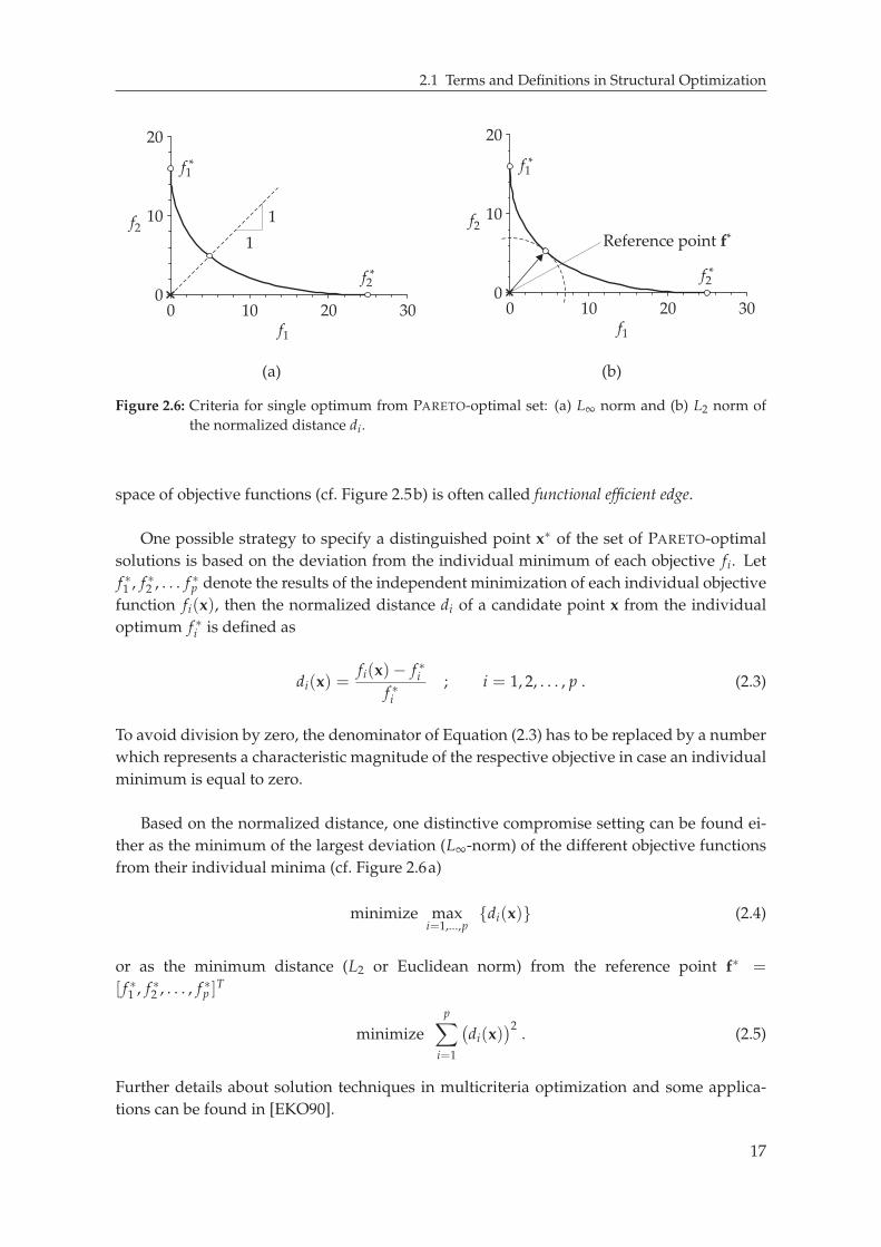
Figure 2.6: Criteria for single optimum from PARETO-optimal set: (a) L∞ norm and (b) L2 norm of
the normalized distance di.
space of objective functions (cf. Figure 2.5b) is often called functional efficient edge.
One possible strategy to specify a distinguished point x∗ of the set of PARETO-optimal
solutions is based on the deviation from the individual minimum of each objective fi. Let
f ∗1 , f ∗2 , . . . f ∗p denote the results of the independent minimization of each individual objective
function fi(x), then the normalized distance di of a candidate point x from the individual
optimum f ∗i is defined as
di(x) =fi(x) − f ∗i
f ∗i; i = 1, 2, . . . , p . (2.3)
To avoid division by zero, the denominator of Equation (2.3) has to be replaced by a number
which represents a characteristic magnitude of the respective objective in case an individual
minimum is equal to zero.
Based on the normalized distance, one distinctive compromise setting can be found ei-
ther as the minimum of the largest deviation (L∞-norm) of the different objective functions
from their individual minima (cf. Figure 2.6a)
minimize maxi=1,...,p
di(x) (2.4)
or as the minimum distance (L2 or Euclidean norm) from the reference point f∗ =
[ f ∗1 , f ∗2 , . . . , f ∗p ]T
minimize
p∑
i=1
(
di(x))2
. (2.5)
Further details about solution techniques in multicriteria optimization and some applica-
tions can be found in [EKO90].
17

CHAPTER 2 STRUCTURAL OPTIMIZATION
2.1.5 Standard Formulation of Optimization Problems
The introduced terms and definitions are summarized to form the standard formulation of
a structural optimization problem with continuous design variables:
minimize f (x) ; x ∈ Rn (2.6a)
such that gj(x) ≤ 0 ; j = 1, . . . , ng (2.6b)
hk(x) = 0 ; k = 1, . . . , nh (2.6c)
xLi ≤ xi ≤ xU
i ; i = 1, . . . , n . (2.6d)
Combining Equations (2.6b-d), the feasible domain C is characterized by
C = x ∈ Rn | gj(x) ≤ 0 ∧ hk(x) = 0 ∧ xL
i ≤ xi ≤ xUi . (2.7)
The set of points defined by Equation (2.6d) constitutes the design space D
D = x ∈ Rn | xL
i ≤ xi ≤ xUi . (2.8)
In this thesis the objective function is always formulated to define a minimization problem.
All inequality constraints are transformed to the form given in Equation (2.6b). Multicriteria
optimization problems are solved either by forming one composite objective function or by
determining a preference function from the set of conflicting objectives. Hence, a unique
solution vector x∗, which defines the optimal design, will be obtained. This solution vector
may either describe a local or a global minimum depending on both the characteristics of the
objective and constraint functions and on the features of the optimization algorithm.
2.1.6 Special Cases of Optimization Problems
Constrained vs. unconstrained optimization. Optimization formulations containing nei-
ther equality nor inequality constraints are called unconstrained optimization problems, all oth-
ers are termed constrained optimization problems. For constrained optimization problems,
the number of equality constraints nh has to be less than or equal to the length of the design
variable vector n, which quantifies the number of degrees of freedom in the optimization
problem. If nh > n and no equality constraint is redundant, the system of equations is
overdetermined, and the formulation of the optimization problem becomes inconsistent i.e. no
solution of the optimization problem exists. There is no limit to the number of inequality
constraints in the formulation of the optimization task; the maximum number of active, non-
redundant constraints at the optimum, however, is limited to the number of design variables
n.
With many optimization algorithms only unconstrained problems can be solved, or un-
constrained problems are at least much easier to handle. Hence, the standard formulation in
Equations (2.6a-d) for constrained problems is often transformed to the unconstrained case
using the Lagrangian function. The formulation of a Lagrangian function will be explained in
detail in Section 2.2.
18

2.1 Terms and Definitions in Structural Optimization
Linear and quadratic programming. In cases where the functions f (x), gj(x) and hk(x)
describing the objective, inequality, and equality constraints, respectively, are linear and/or
quadratic functions only, the optimization problem can be solved very efficiently. On this
account, a distinction is drawn between linear programming
minimize f (x) = eTx ; x ∈ Rn (2.9)
such that gj(x) = A x + b ≤ 0 ; j = 1, . . . , ng
hk(x) = C x + d = 0 ; k = 1, . . . , nh
xLi ≤ xi ≤ xU
i ; i = 1, . . . , n
and quadratic programming
minimize f (x) =1
2xTQ x + eTx ; x ∈ R
n (2.10)
such that gj(x) = A x + b ≤ 0 ; j = 1, . . . , ng
hk(x) = C x + d = 0 ; k = 1, . . . , nh
xLi ≤ xi ≤ xU
i ; i = 1, . . . , n .
Because of their beneficial features, linear and quadratic programming schemes are often
used as formulations for sub-problems in sequential solution procedures. These solution
techniques are called sequential linear programming (SLP) or sequential quadratic programming
(SQP) methods, respectively.
Nonlinear problems. In general, the functions f (x), gj(x) and hk(x) are nonlinear in the
design variables x. If this is the case for at least one of these functions, the optimization
problem is called nonlinear.
Convex vs. non-convex problems. To distinguish convex and non-convex problems, the
concept of convexity has to be established for the set of feasible designs (feasible domain)
and for the objective function. A collection of points S is called a convex set if the line segment
joining any two points x1, x2 ∈ S lies entirely in S . This notion can be represented by
x1, x2 ∈ S ⇒ α x1 + (1 − α) x2 | 0 < α < 1 ⊂ S (2.11)
or graphically as depicted in Figure 2.7.
A function f (x) is called a convex function if first, it is defined on a convex set x ∈ S ,
and second, it lies below the line segment linking any two points on f (x). This geometrical
characterization (cf. Figure 2.8) of a convex function can be formulated mathematically as
f(
α x1 + (1 − α) x2)
≤ α f (x1) + (1 − α) f (x2) ; 0 < α < 1 . (2.12)
In practice the fulfillment of the inequality in Equation (2.12) will be difficult to prove be-
cause an infinite number of combinations of two points has to be analyzed. Alternatively,
the convexity of a function can be checked using the Hessian matrix (or simply Hessian) of
19

CHAPTER 2 STRUCTURAL OPTIMIZATION
(b)(a)
x2
x1
x2x1
Figure 2.7: (a) Convex set and (b) non-convex set in 2D space.
the function f (x) if f (x) is twice differentiable. The Hessian H is a symmetric n × n ma-
trix containing the second derivatives of f (x) with respect to the independent variables xi.
Consequently, it is also denoted by ∇2 f .
H(x) = ∇2 f (x) =
∂2 f (x)
∂x1∂x1
∂2 f (x)
∂x1∂x2. . .
∂2 f (x)
∂x1∂xn
∂2 f (x)
∂x2∂x1
∂2 f (x)
∂x2∂x2. . .
∂2 f (x)
∂x2∂xn...
......
∂2 f (x)
∂xn∂x1
∂2 f (x)
∂xn∂x2. . .
∂2 f (x)
∂xn∂xn
(2.13)
It can be shown that f (x) is convex if and only if the Hessian is positive semidefinite for
every point x ∈ S .
The optimization problem in Equations (2.6a-d) is called a convex problem if both the
objective function and the feasible domain characterized by the constraints are convex. To
(a) (b)
0
10
20
30
40
2 4 6 8 10
f x( )
f x( )1
α=1α=0
f x( )2
f x( )
0
10
20
30
40
2 4 6 8 10
f x( )1f x( )2
Figure 2.8: (a) Convex and (b) non-convex function f (x) for a 1D problem.
20

2.2 Optimality Conditions
Feasible domain
g1( )=0x
g2( )=0x
g3( )=0xg4( )=0x
Figure 2.9: Convex feasible domain defined by non-convex inequality constraints.
identify whether the feasible domain is a convex set, the following statements will be help-
ful:
⋄ If a function g(x) is convex, then the set S = x ∈ Rn | g(x) ≤ 0 is convex.
⋄ If an equality is used to delimit a set of points S = x ∈ Rn | h(x) = 0, then S is
convex if and only if h(x) is linear.
⋄ A set defined as intersection of several convex sets is always convex.
Relating these statements leads to a possible identification of a convex optimization
problem: If a problem has a convex objective function f (x), convex inequality constraint
functions gj(x), and linear equality constraint functions hk(x), then it is a convex optimiza-
tion problem. This, however, is not a necessary condition for a convex problem because a
feasible domain defined by non-convex inequality constraints (cf. g1 and g2 in Figure 2.9)
can still be convex.
A convex problem has the important feature that it has only one minimum i.e. a local
minimum is also a global minimum. Although convex problems are rarely encountered in
engineering practice, this special trait is often used in solution techniques applying sequen-
tial (convex) approximations to the true optimization problem e.g. SQP. Further details on
optimization algorithms using convex approximations are given in Section 2.3.
2.2 Optimality Conditions
In this section, several criteria are discussed to decide whether an investigated point repre-
sents a local or a global minimum for the optimization problem. Apart from the obvious
requirement that the solution of the optimization problem x∗ must yield the lowest feasible
value for the objective function i.e. there is no other point x′ within the feasible domain Cresulting in a better objective value
f (x∗) ≤ f (x′) ∀ x′ ∈ C , (2.14)
21

CHAPTER 2 STRUCTURAL OPTIMIZATION
x
f x( )C
B
A
Figure 2.10: Minimum (A), saddle point (B), and maximum (C) for a 1D problem.
further conditions for an optimum point can be identified which prove more helpful for
many solution techniques. But before these conditions are introduced, two different types of
optimal points are distinguished: global and local minima. The formulation in Equation (2.14)
describes a global optimum since no better solution can be determined within the entire
feasible domain C. If the condition only holds in a neighborhood N (x∗) of the candidate
point x∗
f (x∗) ≤ f (x′) ∀ x′ ∈ N (x∗) (2.15)
with N (x∗) = x ∈ Rn | ‖x − x∗‖ < ε ∧ ε > 0 , (2.16)
the point x∗ is a local optimum. If strict inequality holds in Equation (2.14) or (2.15), the
respective minimum point is termed isolated (global or local) minimum.
In view of the strongly unequal complexity of the formulation of optimality criteria, two
different cases are distinguished in the following: unconstrained and constrained optimiza-
tion.
Unconstrained Problems. As a necessary condition for a point to be a candidate for a min-
imum, it must be a stationary point i.e. the gradient of the objective function evaluated at x∗
must vanish.
∇ f (x∗) = 0 (2.17)
with
∇ f (x) =∂ f (x)
∂x=
[
∂ f (x)
∂x1,
∂ f (x)
∂x2, · · · ,
∂ f (x)
∂xn
]T
(2.18)
Yet another condition must be fulfilled to exclude the cases of maxima or saddle points as de-
picted in Figure 2.10 – points that will also fulfill the necessary condition of Equation (2.17).
To identify the case of a minimum, information about the second partial derivatives at the
stationary points is used. If the Hessian, as defined in Equation (2.13), is positive definite at
a stationary point, this point marks a minimum. This is a sufficient condition for a minimum
of the unconstrained optimization problem.
22

2.2 Optimality Conditions
x1
x2 Contours ( ) = const.f x
g2( ) 0x =
g1( ) 0x =
Feasible domain
gj( ) 0x ≤
Optimum *x
f( )x*
g1( )x*
g2( )x*
f( )x*
f( )x*
g2( )x*λ2
−
g1( )x*λ1
Figure 2.11: Geometrical interpretation of Equation (2.21).
Constrained Problems. For constrained optimization problems, the necessary condition
as formulated in Equation (2.17) may not hold if at least one constraint is active at the opti-
mum (cf. Fig 2.4a). Hence, a different necessary condition must be formulated for the con-
strained optimization case. The following requirements form the so-called KUHN-TUCKER
conditions, which represent the necessary conditions for a constrained optimum.
1. x∗ ∈ C (2.19)
2. λ∗j gj(x∗) = 0 ; j = 1, . . . , ng (2.20)
3. ∇ f (x∗) +
ng∑
j=1
λ∗j ∇gj(x∗) +
nh∑
k=1
µ∗k∇hk(x∗) = 0 ; λ∗
j ≥ 0 (2.21)
As an obvious prerequisite, exclusively feasible designs are allowed as candidate points
for the optimum as formulated in Equation (2.19). According to Equation (2.20), the scalar
parameters λ∗j are identically zero if the corresponding inequality constraint is not active
i.e. gj(x∗) < 0. After the following rearrangement
− ∇ f (x∗) =
ng∑
j=1
λ∗j ∇gj(x∗) +
nh∑
k=1
µ∗k∇hk(x∗) , (2.21’)
the third condition can be understood geometrically as depicted in Figure 2.11: The gra-
dients of all inequality and equality constraints, evaluated at a stationary point and scaled
with factors λ∗j and µ∗
k , respectively, sum up to the negative gradient of the objective func-
tion. Only gradients of active constraints are included in the vector sum since the gradients
of inactive constraints are scaled to zero length by their corresponding λj as stipulated in
Equation (2.20). A closer look at Equation (2.21) reveals that this necessary condition for
23

CHAPTER 2 STRUCTURAL OPTIMIZATION
x1
x2
A
B
C
g( ) 0x =
Feasible domain
g( ) 0x ≤
f( ) = const.x
Figure 2.12: Stationary points for a non-convex problem.
stationary points is in fact also the gradient of a yet to determine function similar to Equa-
tion (2.17). The function corresponding to the objective f (x) of the unconstrained case is the
antigradient of Equation (2.21) with respect to the design variables x, termed the Lagrangian
function L
L(x, λ, µ) = f (x) +
ng∑
j=1
λjgj(x) +
nh∑
k=1
µkhk(x) (2.22)
with the so-called Lagrangian multipliers λj and µk. The Lagrangian function combines both
objective and constraint functions to a single function which has the same solution as the
original problem formulation since the terms added to the objective are all equal to zero
at the optimum. Furthermore the Lagrangian function transforms the constrained into an
unconstrained optimization problem.
The KUHN-TUCKER conditions are necessary conditions only under a certain restriction
called constraint qualification. The constraint qualification excludes those cases where non-
redundant active constraints are linearly dependent. In such cases, constrained minima
that do not fulfill the KUHN-TUCKER conditions are also possible. Even when constraint
qualification is ensured, the KUHN-TUCKER conditions are necessary, but in general not
sufficient for optimality as illustrated in Figure 2.12. Although all three points A, B, and C
fulfill the KUHN-TUCKER conditions, only points A and C are minima (a local and a global
minimum, respectively). For convex problems however, a point that fulfills Equations (2.19)-
(2.21) is a global minimum. Hence, the KUHN-TUCKER conditions are both necessary and
sufficient for a minimum of convex problems.
For the general case of non-convex problems, an additional criterion is needed as suf-
ficient condition for optimality. This sufficient condition for the constrained case is estab-
lished by use of the Hessian of the Lagrangian function in analogy to the procedure in un-
24

2.3 Optimization Algorithms
constrained optimization.
∇2L(x, λ, µ) = ∇
2 f (x) +
ng∑
j=1
λj∇2gj(x) +
nh∑
k=1
µk∇2hk(x) (2.23)
A point x∗ that satisfies the KUHN-TUCKER conditions is a minimum if
sT[
∇2L(x∗, λ∗, µ∗)
]
s > 0 (2.24)
for all s 6= 0 such that
sT∇gj(x∗) = 0 for all active constraints with λ∗
j > 0 (2.25)
sT∇gj(x∗) ≤ 0 for all active constraints with λ∗
j = 0 (2.26)
sT∇hk(x∗) = 0 . (2.27)
Equations (2.25) through (2.27) determine the vectors s to be tangential to all active con-
straints at x∗. Hence, Equation (2.24) stipulates that the Hessian of the Lagrangian function
must be positive definite for all s lying in the hyperplane tangent to the active constraints
at the candidate point x∗. In this context, two special cases ought to be addressed: First,
the fact that Equation (2.24) is not met at a candidate point does not imply that this point is
not a minimum (like in case of a plateau at the minimum). However, the case of an isolated
minimum is ruled out. Second, if the total number of active constraints (incl. at least one
inequality) at a point that complies with the KUHN-TUCKER conditions is equal to the num-
ber of design variables n, the only solution to Equations (2.25) through (2.27) is s = 0 and
thus Equation (2.24) is not valid. Still, these points are (local or global) minima. An example
for this case is depicted in Figure 2.11, where the number of active constraints matches the
number of design variables n = 2.
2.3 Optimization Algorithms
The solution of optimization problems has been addressed by many contributions from dif-
ferent communities viz. mathematicians, engineers, computer scientists, and economists.
Consequently, the range of available algorithms is about as broad as their possible appli-
cations [Van84, Evt85, Min86, Fle87, BSS93, BGLS97, NW99]. Due to the conflicting needs
depending on the different problem types, there is no “one fits all” method that perfectly
suits all possible optimization tasks. The appropriate solution strategy must be chosen on
the basis of individual properties in distinctive features e.g. constrained vs. unconstrained,
convex vs. non-convex problem, discrete vs. continuous optimization, problem size (number
of design variables n), or simply the response values available for the governing functions
(objective and constraints). If these functions are known explicitly and they are twice differ-
entiable, the optimum points can be determined analytically using Equations (2.19) through
(2.21) and (2.24) through (2.27). If inequality constraints are present in the formulation of the
problem, the set of active constraints must be determined by means of a case differentiation.
In most engineering problems, however, the objective and constraints cannot be for-
mulated explicitly and thus can only be evaluated pointwise by solving a linear system of
25

CHAPTER 2 STRUCTURAL OPTIMIZATION
equations e.g. using the finite element method [ZT05]. In this case, the problem has to be
solved by some iterative optimization technique and the most suitable algorithm will de-
pend, amongst other criteria, on whether higher order information can be obtained for the
pointwise determined response values, namely first or second derivatives with respect to
the design variables (gradient vector and Hessian, respectively). Two fundamentally differ-
ent concepts can be distinguished:
⋄ A descent algorithm tries to find the optimum by descending to the lowest point in a
“local valley” (i.e. the convex neighborhood around the starting point). This search
involves the determination of a search direction s(l) at each current iterate x(l) along
which a new iterate x(l+1) is appointed by a line search i.e. a one-dimensional optimiza-
tion with α as independent variable.
x(l+1) = x(l) + α s(l) ; α > 0 (2.28)
This new design point x(l+1) is then investigated and a new search direction s(l+1)
is established. This iterative procedure is repeated until some stopping criterion is
fulfilled (e.g. the change in the design variables becomes very small or the objective
does not decrease in search direction). The diverse descent algorithms differ in the
way the search direction s is established and in the technique used to specify the step
size parameter α. This category of algorithms is in general very efficient if first, second,
or higher order information is available for determination of the search direction.
⋄ According to the second concept, algorithms sample a set of points simultaneously.
Based on this set of sampling points either the best element is picked to define the
optimum or approximation models (e.g. polynomial approximations) for the response
values are built. These approximations are used as surrogate for the original functions
to solve the optimization problem. Some algorithms of this class also allow for a se-
quential approach as well where further sets of sampling points are determined using
information gained from each previous set until a stopping criterion is met. Using this
second category of algorithms, a more global search is conducted – increasing chances
to find the global minimum even for non-convex problems.
Unfortunately, the choice of algorithms is often limited for the designing engineer since
commercially available program packages usually provide only a small selection of meth-
ods if there are any options at all. Additionally, the underlying analysis code (usually a
finite element code) will restrict the choice dependent on the available sensitivities as in-
dicated above. Often no more than zero-order information is available for the response
values. Hence, gradients would have to be determined through finite differences which sig-
nificantly increase computational effort (at least n + 1 analyses are needed to evaluate one
gradient vector).
In this text, a classification of optimization algorithms based on two characteristics is
introduced and depicted in the matrix of Table 2.1. On the one hand, the necessary or-
der of information (zero-order, first-order or second-order) allows for a proper categoriza-
tion of optimization algorithms depending on the code that is used to evaluate the system
26

2.3 Optimization Algorithms
Tab
le2.1
:C
lass
ifica
tio
no
fo
pti
miz
atio
nal
go
rith
ms.
So
lvin
gu
nco
nst
rain
edp
rob
lem
sS
olv
ing
con
stra
ined
pro
ble
ms
1Dp
rob
lem
sn
Dp
rob
lem
sP
rim
alm
eth
od
sT
ran
sfo
rmat
ion
met
ho
ds
zero
-ord
erIn
terv
alse
arch
Gri
dse
arch
Gri
dse
arch
Pen
alty
met
ho
ds
Po
lyn
om
ial
inte
rpo
lati
on
Mo
nte
Car
lora
nd
om
sear
ch
Mo
nte
Car
lora
nd
om
sear
ch
Du
alm
eth
od
s
DiR
ect
alg
ori
thm
Ev
olu
tio
nar
yst
rate
gy
GA
US
S/
SE
IDE
LG
enet
ical
go
rith
m
PO
WE
LL
’sm
eth
od
,
HO
OK
E-J
EE
VE
S’
met
ho
d
Co
mp
lex
met
ho
d(B
OX
)
Sim
ple
xm
eth
od
(NE
LD
ER
,
ME
AD
)
firs
t-or
der
Po
lyn
om
ial
inte
rpo
lati
on
Co
nju
gat
eg
rad
ien
t
(FL
ET
CH
ER
,R
EE
VE
S)
Gen
eral
ized
red
uce
d
gra
die
nts
LA
GR
AN
GE
met
ho
ds
(SQ
P–
qu
asi
NE
WT
ON
)
Bis
ecti
on
Ste
epes
td
esce
nt
Fea
sib
led
irec
tio
ns
Pen
alty
met
ho
ds
SL
PD
ual
met
ho
ds
seco
nd-
orde
rN
EW
TO
Nm
eth
od
Co
nju
gat
eg
rad
ien
t
(HE
ST
EN
ES,
ST
IEF
EL
)
LA
GR
AN
GE
met
ho
ds
(SQ
P–
full
NE
WT
ON
)
NE
WT
ON
met
ho
dP
enal
tym
eth
od
s
Du
alm
eth
od
s
27

CHAPTER 2 STRUCTURAL OPTIMIZATION
characteristics. On the other hand, a distinction is drawn between solution techniques for
constrained and for unconstrained problems. The algorithms used for unconstrained prob-
lems are again subdivided into a class especially suited for 1D problems (i.e. problems with
only one unknown) and n-dimensional problems. Unconstrained optimization problems
with only one design variable are rarely encountered in engineering practice. However, this
special class of algorithms plays an important role in many solution techniques for multi-
dimensional problems using a line search during optimization. The related methods will
be particularized in the next section. Within the approaches used to solve constrained op-
timization tasks, primal and transformation methods are distinguished. Primal methods solve
the original optimization problem with only the design variables as independent variables
whereas transformation methods convert the original formulation into another type (usually
an unconstrained formulation) which is easier to solve but also introduces additional inde-
pendent variables to solve for. Details about the different transformations are given later in
the respective sections in which the key features of some preferred algorithms presented in
Table 2.1 are discussed.
As a consequence of the broad variety of algorithms presented in the literature, Table 2.1
can only present a selection of commonly applied optimization methods for engineering
problems. In the remainder of this section a short discussion of some basic features is given.
For an in-depth discussion of the algorithms addressed in this text and further numerical
optimization techniques, the reader is referred to the cited literature.
2.3.1 Direct Search Methods
Direct search methods use only zero-order information about the governing equations to
find the desired minimum. First, algorithms for 1D minimization will be presented followed
by search methods that apply to multidimensional problems.
Interval search. One example for the class of direct search methods is the interval search.
The basic idea is to gradually reduce the interval in which the minimum lies to a sufficiently
low width. If a function f (α) has only one minimum in the interval under investigation
(a unimodal function), interval search can be applied to reduce the possible range for the
minimum without any requirements on continuity or differentiability of the function. If
values for the objective function f have been computed at four different points α1, α2, α3, and
α4 of the interval [α1, α4], a subinterval can be determined that does not contain the minimum
and hence will be left out for subsequent investigations. As a consequence, the interval
containing the minimum is repeatedly scaled down by evaluating the function values at the
boundaries of each interval.
A very efficient way to choose each interval size can be derived using the golden sec-
tion method because each iteration to reduce the interval size requires only one additional
function evaluation. To achieve this favorable behavior the individual subinterval ranges
∆a = αa+1 − αa with a = 1, 2, 3 must fulfill the condition
∆1
∆2=
∆3
∆2= γ with γ =
√5 + 1
2≈ 1.618 . (2.29)
28

2.3 Optimization Algorithms
For each iteration step, one subinterval of the previous segmentation can be “reused” and
only one additional intermediate point αx must be evaluated to regain three (smaller) subin-
tervals. Using this scheme for the subdivision of the intervals, the rate of interval sizes in
subsequent steps is 1/γ ≈ 0.618. Hence, the remaining range of uncertainty for the mini-
mum after m iteration steps can be computed in advance to be (1/γ)m relative to the initial
interval size.
Polynomial Interpolation. Another efficient technique for one-dimensional optimization
is to approximate the true objective function f (α) by a polynomial p(α). The minimum of
the approximation can be found analytically using the first and second derivative of the
polynomial. The procedure begins with evaluating f (α) at several points. The information
gained at these points (which can also include higher order information) is then used to
fit the polynomial. The optimum of this polynomial, which is used as an estimate for the
optimum of f (α), can be determined analytically.
To identify the optimum α∗ of the commonly applied quadratic polynomial p(α)
p(α) = c0 + c1 α + c2 α2 with∂p(α)
∂α= c1 + 2 c2 α (2.30)
∂p(α)
∂α
∣
∣
∣
∣
α∗= 0 ⇒ α∗ = − c1
2 c2, (2.31)
the parameters c1 and c2 must be determined. This can be realized with three responses of
the original function f1, f2, and f3 at α1, α2, and α3, respectively
c2 =
f3 − f1
α3 − α1− f2 − f1
α2 − α1
α3 − α2, c1 =
f2 − f1
α2 − α1− c2 (α1 + α2) (2.32)
or two response values f1, f2 and one gradient f ′1 at α1 and α2, respectively
c2 =
f2 − f1
α2 − α1− f ′1
α2 − α1, c1 = f ′1 − 2 c2 α1 . (2.33)
For the parameter c0 no formulas are given because it does not influence the position of the
optimum α∗ as shown in Equation (2.31).
The polynomial interpolation method has the advantage of requiring only few function
evaluations. The quality of the obtained estimate for the minimum, however, strongly de-
pends on the accuracy of the approximation p(α) which can be quite poor especially for
highly nonlinear functions f (α). Although the procedure is not restricted to 1D minimiza-
tion, the number of function evaluations to determine the free parameters of multidimen-
sional polynomials rapidly increases with the number of design variables. While a quadratic
polynomial in 1D requires three response values to fit the free parameters, a fully quadratic
polynomial in 3D already needs ten function (or gradient) evaluations. For this reason, mul-
tidimensional problems are usually solved by other approaches.
29

CHAPTER 2 STRUCTURAL OPTIMIZATION
x2
x1
Result of grid search
Contours of objective
Figure 2.13: Grid search for an unconstrained 2D problem.
Grid search. This method is one of the simplest optimization schemes possible. The design
space is examined through evaluations of the objective and constraints at equally spaced
grid points. The point with the smallest sampled value for the objective that satisfies all
constraints is accepted as the best solution (cf. Figure 2.13). This method is computationally
very expensive and the effort required increases exponentially with the number of design
variables. If the points are not positioned on a grid but randomly spread over the design
space (Monte Carlo random search), the computational effort is decoupled from the number of
design variables. Despite the costs for both methods, the location of the optimum will only
roughly be assessed depending on the grid spacing or the number of Monte Carlo points,
respectively. Since these optimization schemes are not bound to a local “valley”, there is a
chance to find the global minimum – but at a high price.
DiRect algorithm. The name of this method is a shortening of the phrase “dividing rect-
angles” and already suggests the underlying idea. Similar to the interval search in 1D, the
DiRect algorithm of JONES et al. subdivides the n-dimensional design space into hyperrect-
angles of different sizes [JPS93]. One function evaluation is performed for each hyperrect-
angle at its center point. Then, the hyperrectangles are sequentially redivided according to
the following scheme (cf. Figures 2.14 and 2.15) until the algorithm converges to a solution.
In the figures, the current approximation for the minimum fmin after each iteration step is
marked with a white circle.
1. To start the algorithm, the originally hyperrectangular design space D as defined in
Equation (2.8) is normalized to form a unit hypersquare D = x ∈ Rn | 0 ≤ xi ≤
1 ; i = 1, . . . , n with center point c as depicted in Figure 2.14.
The algorithm works in this normalized space, referring to the original space only
30

2.3 Optimization Algorithms
x2
c
x1
x2
x1
Normalized design space
(1.) − (2.)
(4.) − (5.) (6.)
Additional points along
each dimension
x2
x1
x2
x1
Subdivision along i* Further subdivisions
(3.)
Contours of
objective
⅓ e1
⅓ e2
Figure 2.14: Initialization of the DiRect algorithm for a 2D problem.
when evaluating the objective function defined on D. Thus, the function call f (c)
denotes the evaluation of c ∈ D that corresponds to c ∈ D.
2. Evaluate the objective function at the center point and set current minimum to fmin =
f (c).
3. Determine response values of the objective for all points defined by c ± 13 ei where
ei are the n unit vectors of the normalized design space. As a result, two additional
sampled points are obtained along each dimension i. Store the smallest sampled value
as new current minimum fmin.
4. Based on the smaller value of the two additional functional responses per dimension
(Step 3), establish a ranking for the different dimensions, start with dimension i∗ that
contains the lowest sampled response fmin.
5. According to this ranking, subdivide the hypersquare into smaller hyperrectangles
starting in dimension i∗. Along this dimension, split the hypersquare into three
31

CHAPTER 2 STRUCTURAL OPTIMIZATION
x2
x1
x2
x1
x2
x1
x2
x1
x2
x1
x2
x1
x2
x1
x2
x1
New subdivision Potentially optimal rectangles
After
initialization
Iteration 1
Iteration 2
Iteration 3
Figure 2.15: Iteration steps (6.) – (8.) of the DiRect algorithm for a 2D problem.
32

2.3 Optimization Algorithms
equally sized hyperrectangles such that c ± 13 ei∗ are the center points of the new hy-
perrectangles.
6. Continue to subdivide the central hyperrectangle, which still contains more than one
point, along the second dimension of the ranking. Repeat this procedure until the cen-
ter hyperrectangle has been divided along each dimension. Now, each hyperrectangle
contains only one point (located at its center point). After this initial segmentation of
the hypersquare, start the iteration.
7. For each iteration step, the DiRect algorithm will identify potentially optimal hyper-
rectangles for further subdivisions.
A hyperrectangle is potentially optimal if there is no hyperrectangle of the same size
or bigger with a smaller response value for its center point. According to [JPS93], the
size of a hyperrectangle is measured by the distance of its center point to the vertices.
Identify all potentially optimal hyperrectangles, and divide each of those into three
equally sized hyperrectangles. The division is executed only along the longest dimen-
sion(s) of the hyperrectangle. This restriction ensures that the rectangles will shrink
in every dimension. If the potentially optimal hyperrectangle is a hypersquare, then
divisions must be performed along all sides, as in the initial step.
8. Evaluate the objective function at the center points of all new hyperrectangles and
update fmin.
9. If the stopping criteria are not met yet, begin the next iteration step with identification
of potentially optimal hyperrectangles (Step 7).
x2
x1
Figure 2.16: DiRect algorithm after eight iterations and 85 function evaluations.
33

CHAPTER 2 STRUCTURAL OPTIMIZATION
Typical stopping criteria are a maximum number of iterations or function evaluations.
To stop the iteration if no change is obtained in fmin or in the corresponding design
variables from one iteration to the other, will in general not lead to the desired opti-
mum as the DiRect algorithm might behave “idle” during several iterations before a
new optimal point is detected.
Figure 2.16 shows the result after eight iterations of the example introduced in Fig-
ure 2.15. To find the approximation for the optimum (marked with a white circle), the
objective function was evaluated 85 times.
The set of potentially optimal hyperrectangles always includes the largest hyperrectan-
gle which will be split during the next iteration step. In case several hyperrectangles are
concurrently the largest, one of these hyperrectangles belongs to the potentially optimal set.
As a consequence, the DiRect algorithm converges to the global optimum at the expense of
an exhaustive search requiring many function evaluations. It is suitable for problems with
a highly nonlinear objective function for which zero order information is cheap to evaluate.
Further details about the DiRect algorithm can be found in [Jon01].
Evolutionary strategies and genetic algorithms. These stochastic optimization methods
imitate evolution in the biological sense and hence represent a numerical adoption of DAR-
WIN’s principle of “survival of the fittest”. The optimal design evolves by means of sequen-
tial selection, mutation, and recombination starting with an initial population of design points
that usually consists of randomly sampled individuals (cf. Monte Carlo random search). “Se-
lection” means that from each population a subset of individuals is chosen as archetypes for
the next generation. The terms “mutation” and “recombination” denote different methods
to form offspring for a selection of individuals.
Mutation diversifies a parent design by changing an arbitrary entry of its numerical de-
scription. This means that a randomly selected design information is spoiled. One example
for mutation, which is often applied to real-valued design vectors, is a random variation.
Typically, a Gaussian normal distribution with mean zero and different standard deviations
σi for each dimension of the design space is used.
x(l+1)i = x
(l)i + N(0, σi) ; i = 1 . . . n (2.34)
As a consequence of this formulation, small mutations are more likely to occur than greater
changes.
For recombination, two selected parents x(l) and z(l) are both split at the same position j
and reassembled cross-over to form two new individuals x(l+1) and z(l+1).
x(l+1) =
x(l)1...
x(l)j
z(l)j+1...
z(l)n
; z(l+1) =
z(l)1...
z(l)j
x(l)j+1...
x(l)n
(2.35)
34

2.3 Optimization Algorithms
The probability of “survival” of the newly generated individuals depends on their fitness
which takes into account the objective function and constraints. Accordingly, the fittest are
kept with high probability, the worst are rapidly discarded.
The basic difference between genetic algorithms and evolutionary strategies lies in the
description of each individual, the so-called gene. For genetic algorithms, each design is
coded in form of a binary string to allow “genetic” operators like mutation and recombi-
nation to apply to any part of the gene without any knowledge of its physical meaning. In
contrast, evolutionary strategies constitute their genes as a vector of real-valued parameters
which are altered primarily by mutation. This rather slightly perturbs the individual pa-
rameters of the genes in a useful way. Hence, evolutionary strategies are mostly applied to
continuous problems while genetic algorithms are a preferred tool for discrete optimization.
Many different configurations exist for both methods [BS93, BFM96]. The underlying
optimization scheme, however, is basically the same for all procedures:
1. Specify an initial population i.e. a set of np individuals xp with p = 1 . . . np in the
design space.
2. Evaluate the objective function and constraints at all points xp to assign their fitness
value.
3. Select members of the parent population with adequate fitness as archetypes for a
child population.
4. Create a child population xc with c = 1 . . . nc by means of reproduction and mutation.
5. Evaluate the fitness for all points xc.
6. Check stopping criterion. If it is not met, proceed with Step 3 to set up a new genera-
tion.
To assess this class of algorithms the following observations can be made. They need only
zero order information but require numerous function evaluations. They can easily handle
nonlinear problems even with functions of discrete variables and tend to detect the global
optimum after sufficient iterations. The problem is to specify a suitable stopping criterion
since the optimization might be stalling for several iterations before further improvement
is attained. Consequently, the only generally applicable stopping criterion is to limit the
number of iterations or evaluations.
When applied to multicriteria problems, evolutionary strategies and genetic algorithms
are capable of finding several points of the PARETO-optimal set during one optimization
run [Deb01]. These special traits make this class particularly suited for applications with
discrete design variables and for highly nonlinear problems. To assure that the computa-
tional effort remains within acceptable limits, response values have to be rather cheap to
evaluate.
35

CHAPTER 2 STRUCTURAL OPTIMIZATION
2.3.2 Gradient Methods
With the help of first order information for the objective and constraint functions, more
efficient algorithms can usually be formulated to find the solution of the optimization prob-
lem. If gradients are readily available, this will in general reduce the number of function
evaluations needed to solve the optimization task as already indicated for the polynomial
interpolation approach. But even if the first order information must be determined via fi-
nite differences, gradient methods still perform better than direct search methods in some
applications.
Steepest descent method. The most intuitive approach for descent methods is to use the
direction of the steepest descent (i.e. the opposite direction of the gradient of the objective) to
search for the optimum. Hence, the search direction s(l) in Equation (2.28) for each iteration
step l is calculated from
s(l) = −∇ f(
x(l))
. (2.36)
The step size α is determined by a line search method. If the line search found the minimum
in the search direction s(l), the next search direction s(l+1) will be orthogonal to s(l). This
feature leads to a poor convergence rate of the steepest descent method when the underlying
problem is badly scaled (cf. Figure 2.17).
Conjugate gradient method. In order to overcome the aforementioned poor convergence
behavior of the steepest descent method, FLETCHER and REEVES developed the conjugate
gradient method [FR64] which requires only a minor change in the determination of the
search direction. The initial search direction s(0) is chosen to be the steepest descent direction
of Equation (2.36). All subsequent search directions are determined by
s(l+1) = −∇ f(
x(l))
+ β(l) s(l) with β(l) =
∥
∥
∥∇ f(
x(l))
∥
∥
∥
∥
∥∇ f(
x(l−1))∥
∥
2
, (2.37)
x1
Contours of objective
x2 Scaled x2
Scaled x1
Figure 2.17: Influence of scaling on convergence behavior of the steepest descent method.
36

2.3 Optimization Algorithms
x1
x2
g2( ) 0x =
g1( ) 0x =
s( )l
f( )x( )l
g1( )x( )l
Usable sector
Feasible sector
Usable-feasible sector
f( ) = const.x Tangent to ( )f x( )lTangent to ( )x( )lg1
Figure 2.18: Feasible and usable search directions for a 2D problem with one active constraint.
where the direction of the previous step scaled by the factor β(l) is added to the current
negative gradient. The scaling factor is defined using the L2 norm of the gradients at the
current design point and the gradient from the previous iteration step. By means of this
enhancement, the conjugate gradient method finds the optimum of a quadratic function of
n design variables in n or fewer iterations.
Method of feasible directions. To allow for solution of constrained problems, an enhance-
ment of descent methods described earlier is presented next: the method of feasible direc-
tions. The initial design point is imposed to be a feasible design. As long as the iteration
remains inside the feasible domain, the search direction is determined as for the uncon-
strained case. If during the iteration a constraint j becomes active, the next search direction
s(l) must satisfy two conditions:
1. The search direction must be feasible i.e. it must point into the feasible domain.
∇gj
(
x(l))T
s(l) ≤ 0 (2.38)
2. The search direction must be usable i.e. the objective must be reduced in this direction.
∇ f(
x(l))
s(l)< 0 (2.39)
As a consequence, the new search direction must fall into the cone spanned by the tan-
gents to the active constraint and the contour of the objective as illustrated in Figure 2.18.
Search directions close to the constraint tangent are in general not advantageous because for
37

CHAPTER 2 STRUCTURAL OPTIMIZATION
nonlinear constraints even small steps in this direction would result in infeasible designs.
Consequently, a “push-off” factor θ > 0 is introduced to enhance the search direction.
∇gj
(
x(l))T
s(l) + θ ≤ 0 (2.40)
For further details on the choice of θ and its influence on convergence behavior of the
method, it is referred to [VM73]. An extension of the method to cope with initially infeasible
designs is described in [Van84].
2.3.3 NEWTON and Quasi NEWTON Methods
Newton methods use second order information to find the optimum. They are derived from
the linearization of the stationary condition in Equation (2.17). The linearized stationary
condition of the unconstrained case at some iterate x(l) reads
∇ f(
x(l))
+ ∇2 f(
x(l))
d(l) = 0 with d(l) = x(l+1) − x(l) , (2.41)
where d(l) denotes the vector that describes the next iteration step. Solving Equation (2.41)
for the next iteration point x(l+1) yields
x(l+1) = x(l) −[
∇2 f(
x(l))
]−1∇ f(
x(l))
, (2.42)
which represents the update formula for a classical NEWTON-RAPHSON method to find the
roots of Equation (2.17). Even if the Hessian for the objective ∇2 f(
x(l))
can be determined,
evaluating and inverting it for every iteration step is in general too expensive for practical
applications. Hence, an approximation is used in most cases e.g. by updating the Hessian
only every few iterations assuming that the second derivatives of the objective do not change
as fast as the corresponding zero and first order information. Another possibility to reduce
the computational effort in combination with NEWTON methods is the approximation of the
Hessian by means of first order information only. Due to the different possibilities of approx-
imating the Hessian or its inverse, this leads to a special class of algorithms, the so-called
quasi NEWTON methods. Two prominent members of this class are the DFP method (named af-
ter DAVIDON [Dav59], FLETCHER, and POWELL [FP63]) and the BFGS method (named after
BROYDEN [Bro70], FLETCHER [Fle70], GOLDFARB [Gol70], and SHANNO) [Sha70]. The DFP
method starts with an initial guess A0 for the inverse of the Hessian (usually the identity
matrix A0 = I) which is modified after each iteration step using two correction matrices B(l)
and C(l) such that
A(l+1) = A(l) + B(l) + C(l) (2.43)
with
B(l) =d(l) d(l)T
d(l)Ty(l)
; C(l) = −A(l) y(l) y(l)TA(l)
y(l)TA(l) y(l)
; y(l) = ∇ f (x(l+1)) − ∇ f(
x(l))
. (2.44)
The BFGS method updates an approximation H(l) for the true Hessian rather than its inverse
at every iteration, also starting with an initial guess which, in absence of more information,
is often estimated by the identity matrix H0 = I.
H(l+1) = H(l) + D(l) + E(l) (2.45)
38

2.3 Optimization Algorithms
with
D(l) =y(l) y(l)T
y(l)Td(l)
; E(l) = − H(l) d(l) d(l)TH(l)
d(l)TH(l) d(l)
(2.46)
For both methods the matrices A and H, respectively, must remain positive definite during
the iteration process to allow for convergence of the algorithm. Since poor approximations
for the Hessian might lead to non-convergent behavior of the algorithm, a line search should
always be performed in combination with quasi-NEWTON methods. Derived from the up-
date direction of NEWTON methods
s(l) =[
∇2 f(
x(l))
]−1∇ f(
x(l))
, (2.47)
the search direction for a line search during a quasi-NEWTON iteration can be deduced:
s(l)DFP = A(l)
∇ f(
x(l))
; s(l)BFGS =
[
H(l)]−1
∇ f(
x(l))
. (2.48)
More details about quasi-NEWTON methods can be found e.g. in [Fle87, NW99, Van84].
2.3.4 LAGRANGE Methods
In order to solve constrained optimization problems, the aforementioned NEWTON meth-
ods can also be applied to the Lagrangian function instead of the objective function. The
Lagrangian function transforms the original constrained problem into an unconstrained
problem. The resulting unconstrained problem can then be solved using the techniques
described in the previous sections. Assuming that the set of active inequality constraints
has already been determined for the current iteration step, all active inequality constraints
can be treated as additional equality constraints
gj(x) = 0 ; j = 1 . . . na , (2.49)
where na denotes the number of active inequality constraints at point x. Constraints that are
inactive at the current iterate are neglected for the next step. Using the information about
the active set, the Lagrangian function reads
L(x, µ) = f (x) +
nh+na∑
k=1
µk hk(x) (2.50)
The desired minimum must fulfill the stationary condition for the Lagrangian function i.e.
∂L(x, µ)
∂x= 0 (2.51)
∂L(x, µ)
∂µ= 0 (2.52)
Again, applying the NEWTON-RAPHSON method to find the roots of these equations yields
the linearized forms of Equations (2.51) and (2.52) which can be combined to
∇2 f (x(l)) +
nh+na∑
k=1
µ(l)k ∇
2hk(x(l)) ∇h(x(l))T
∇h(x(l)) 0
[
d(l)
δ(l)
]
= −[
∇L(x(l))
h(x(l))
]
(2.53)
39

CHAPTER 2 STRUCTURAL OPTIMIZATION
with
d(l) = x(l+1) − x(l) ; δ(l) = µ(l+1) − µ(l) (2.54)
In Equation (2.53), the different equality constraints hk(x) are assembled to the vector h(x)
and ∇h(x(l)) denotes the matrix that contains the partial derivatives of each hk(x) with
respect to the design variables x.
∇h(x) =
∂h1(x)
∂x1
∂h1(x)
∂x2· · · ∂h1(x)
∂xn
∂h2(x)
∂x1
∂h2(x)
∂x2· · · ∂h2(x)
∂xn...
......
∂hnh+na(x)
∂x1
∂hnh+na(x)
∂x2· · · ∂hnh+na(x)
∂xn
(2.55)
Equations (2.53) and (2.54) characterize an iterative optimization algorithm called sequential
quadratic programming (SQP) that will iteratively find a stationary point of L(x, µ), the so-
lution of the constrained optimization problem. After each step, the active set at x(l) must
be redetermined for the next iteration. To reduce the computational effort related to the
evaluation of the second derivatives in Equation (2.53), the approximation techniques for
the Hessian described in the preceding section can be applied in an analogous manner. The
only difference is that a line search on the Lagrangian function will not help to stabilize
because its stationary point is not a global minimum, but a saddle point (maximum with
respect to µ and minimum with respect to x). Hence, other techniques must be applied to
ensure convergence [NW99].
2.3.5 Penalty and Barrier Methods
Another possibility to solve a constrained optimization problem is to reformulate the objec-
tive such that the new objective worsens rapidly where constraints are violated. This can be
accomplished by adding a penalty or barrier function to the original objective
f (x, r) = f (x) + P(x, r) , (2.56)
which is also a function of an additional scalar, called the penalty parameter r.
The basic difference between penalty and barrier methods is that the former penalize the
objective only if a constraint is violated (i.e. f (x, r) = f (x) within the whole feasible domain)
whereas the latter do not allow for infeasible designs by means of a singularity at the limit
state gj(x) = 0. Consequently, barrier methods are applicable only to inequality constrained
problems.
A popular example for a penalty function is the quadratic loss function defined as
P(x, r) = r
ng∑
j=1
(
g+j (x)
)2+
nh∑
k=1
(
hk(x))2
(2.57)
40

2.3 Optimization Algorithms
2 4 6 8 100
10
20
30
-10
f x( )
f x,r= ( 0.1)
f x,r= ( 1)
f x,r= ( 10)f x,r= ( 100)
g( )x
Feasible Infeasible
40
(a) (b)
2 4 6 8 100
10
20
30
-10
f x( )
f x,r= ( 0.1)
f x,r= ( 1)
f x,r= ( 10)
f x,r= ( 100)
g( )x
Feasible Infeasible
40
Figure 2.19: Influence of penalty parameter r on approximation quality of (a) penalty and (b) barrier
methods.
with
g+j (x) = max
0 ; gj(x)
. (2.58)
Commonly used barrier functions are the inverse barrier function
P(x, r) =1
r
ng∑
j=1
(
− 1
gj(x)
)
(2.59)
and the logarithmic barrier function
P(x, r) = −1
r
ng∑
j=1
log(
−gj(x))
. (2.60)
Similar to the LAGRANGE formulation, Equation (2.56) transforms the original con-
strained problem into an unconstrained problem. In contrast to the LAGRANGE method,
however, the solution of the penalty formulation in Equation (2.56) is in general not the
same as for the original formulation. If the true optimum lies on the boundary of the feasible
domain, penalty methods will typically yield “optimal” solutions that are located slightly
in the infeasible domain while barrier methods will “back off” into the feasible domain and
thus also miss the true optimum. The difference between the found optimum and the true
minimum strongly depends on the penalty parameter r. As illustrated in Figure 2.19, the
approximation ameliorates for increasing r. Extremely large values for r, however, lead to
numerical problems during optimization. A detailed discussion of advantages and disad-
vantages of both penalty and barrier methods are discussed for instance in [Aro89, BSS93].
41

CHAPTER 2 STRUCTURAL OPTIMIZATION
2.3.6 Approximation Concepts
Seizing the idea used for the method of polynomial interpolation, other approximations to
the original objective function or constraints can be established to find the optimum [BH93].
Dependent on their region of validity, local, mid-range, and global approximations are distin-
guished. While local approximations are only valid in the immediate vicinity of the ob-
served point, mid-range approximations try to predict the original functional response in
a well-defined subregion of the design space. In contrast, global approximations aim at
predicting the characteristics of the functions over the entire design space.
Local approximations are fit based on local information obtained at a single point such as
the functional value, gradient and curvature, respectively. Hence, they are also called single
point approximations. The more information is available (e.g. by means of sensitivity anal-
ysis [Kim90, SCS00]) the better the possible fit will be. Mid-range approximations rely on
information gathered from multiple points. Both local and mid-range approximations form
explicit subproblems (defined on a subregion of the design space) that can be solved analyt-
ically. Accordingly, an iterative solution technique is commonly applied where the solution
of one subproblem provides the expansion point for the next approximation. This iteration
is performed until convergence is achieved. Well-known local approximation methods are
the TAYLOR expansion and the method of moving asymptotes (MMA) [Sva87, Ble93]. A promi-
nent member of the mid-range approximation family is the so-called multipoint approxima-
tion [TFP93].
The simplest local approximation is the linear TAYLOR expansion about current design
x′. In this case, the TAYLOR series is truncated after the linear term. Applied to the objective
function f (x), the linear approximation reads
f (x) = f(
x′)
+n∑
i=1
∂ f (x)
∂xi
∣
∣
∣
∣
x′(xi − x′i) . (2.61)
If the quadratic terms of the TAYLOR series are included in the expansion, the approxima-
tion is improved at the price of requiring curvature information at x′, either determined
analytically or by means of finite differences. This additional computational effort makes
the quadratic Taylor approximation inapplicable to most structural optimization problems.
f (x) = f(
x′)
+n∑
i=1
∂ f (x)
∂xi
∣
∣
∣
∣
x′(xi − x′i) +
1
2
n∑
i=1
n∑
j=1
∂2 f (x)
∂xi ∂xj
∣
∣
∣
∣
x′(xi − x′i)(xj − x′j) (2.62)
As a more general approach for local approximations, which also includes the linear
TAYLOR expansion as a marginal case, the MMA is discussed in brief. A thorough discussion
of MMA and enhanced approaches can be found in [Dao05]. The MMA approximation
f (x) = r′ +n∑
i=1
(
pi
Ui − xi+
qi
xi − Li
)
(2.63)
is convex within the range [Li, Ui] defined by an upper and lower asymptote Li and Ui,
respectively. The position of the asymptotes can be changed from one iteration step to the
42

2.3 Optimization Algorithms
other, a feature motivating the name of this method. The coefficients of Equation (2.63) are
defined as
r′ = f(
x′)
−n∑
i=1
(
pi
Ui − x′i+
qi
x′i − Li
)
(2.64)
pi =
(Ui − x′i)2 ∂ f (x)
∂xi
∣
∣
∣
∣
x′, if
∂ f (x)
∂xi
∣
∣
∣
∣
x′> 0
0 , otherwise
(2.65)
qi =
0 , if∂ f (x)
∂xi
∣
∣
∣
∣
x′≥ 0
− (x′i − Li)2 ∂ f (x)
∂xi
∣
∣
∣
∣
x′, otherwise.
(2.66)
Mid-range and global approximations are based on evaluations of the original func-
tions at a set of points, called sampling points. To yield the best possible approximation,
the sampling points are carefully chosen according to design of experiments (DoE) tech-
niques [Mon01]. The resulting approximations can be used to efficiently study the behavior
of the problem replacing expensive evaluations of the original functions. These approxi-
mations models (also termed metamodels) and related DoE methods are a key issue of the
present work. Therefore, they are thoroughly discussed together with aspects related to
their use in optimization algorithms in Chapters 4, 5, and 6.
43

CHAPTER 2 STRUCTURAL OPTIMIZATION
44

Chapter 3
Stochastic Structural Optimization
The concepts introduced in Chapter 2 imply that all parameters involved are inherently de-
terministic i.e. known, determined, or produced to exactly the value used in the optimiza-
tion process. Obviously, this approach is an idealization of real-life processes, products, and
materials subject to environmental influences. The natural stochastic character is neglected
in most engineering problems for the sake of an easy implementation, reduced numerical
effort, or increased clarity in the problem formulation.
In the context of structural optimization, however, this approach may be very critical.
During optimization, existing redundancies are typically downsized or even eliminated
completely, since any redundancy is a potential source for further improvement. Finally,
the optimized design has no redundancies left to cover inherent uncertainties. In particular
constrained optima are highly sensitive even to small deviations in the governing parame-
ters because any variation in direction of the active constraint leads to an infeasible layout.
In contrast, a robust design, the goal of a stochastic optimization, is characterized by minimal
impact of variations on the system response.
Bearing the formulation of a stochastic optimization problem in mind, some major sta-
tistical measures are introduced first. Subsequently, several formulations for stochastic opti-
mization problems are discussed, followed by a presentation of solution techniques for this
class of problems.
3.1 Basic Statistical Concepts
A design variable or system parameter that exhibits stochastic properties is called a ran-
dom variable. Random variables are denoted by uppercase letters, such as X. All statistical
quantities and functions that characterize a particular random variable are indexed with the
respective uppercase letter. The corresponding lowercase letter x is used to denote a possi-
ble value of X. The set of possible outcomes for X are called the sample space Ω. Any subset
of Ω is called an event.
The character of a random variable X is specified by its probability distribution pX(x). If
X is a discrete variable, pX(x) is often called probability function or probability mass function.
In case of a continuous X, it is termed probability density function. Examples for possible
probability distributions are depicted in Figure 3.1.
45

CHAPTER 3 STOCHASTIC STRUCTURAL OPTIMIZATION
x x
aa b
p x( )P X a p a ( )= =
P a X≤b ≤
p x( )
(a) (b)
Figure 3.1: Probability distribution pX for (a) discrete and (b) continuous random variable X.
The probability distribution quantifies the probability P of a specific event to occur. It is
noteworthy that in the discrete case the value pX(a) represents the probability of the event
X = a whereas for continuous variables the integral over a range of X provides a measure
for probability. Consequently, for continuous X, the probability of occurrence of one distinct
X = a is zero. Probability distributions must have the following properties:
⋄ Discrete x: 0 ≤ pX(xi) ≤ 1 ∀ xi ∈ Ω (3.1)
PX = xi = pX(xi) ∀ xi ∈ Ω (3.2)∑
i
pX(xi) = 1 (3.3)
⋄ Continuous x: pX(x) ≥ 0 (3.4)
Pa ≤ X ≤ b =
b∫
a
pX(x) dx (3.5)
∫
Ω
pX(x) dx = 1 . (3.6)
For the purpose of clarity, only the case of continuous random variables is further elabo-
rated, a detailed discussion on discrete random variables can be found e.g. in [MR03].
A fundamental function in statistics is the cumulative distribution function
C(x) = PX ≤ x =
x∫
−∞
pX(u) du , (3.7)
which quantifies the probability of the event that a random realization of X is smaller than
the value x. Using the inverse of the cumulative distribution function, quantiles of X can
be specified i.e. values xq for which the probability of X being smaller than xq is equal to a
preset probability q
xq = C−1(q) . (3.8)
46

3.1 Basic Statistical Concepts
Two important statistical measures are mean µ and variance σ2, respectively. The mean of a
distribution is also termed expected value and is a measure of its location (or central tendency)
while the variance is a measure of dispersion of a probability distribution.
E(X) = µX =
∫
Ω
x pX(x) dx (3.9)
V(X) = σ2X =
∫
Ω
(x − µX)2 pX(x) dx =
∫
Ω
x2 pX(x) dx − µ2X (3.10)
For engineering problems, the positive square root of the variance, called standard devia-
tion σ, is often the preferred measure for variability because it has the same dimension as
the corresponding random variable X. Additional measures of location and dispersion are
discussed in standard literature on statistics, for instance [Ros87, MR03, Sac04].
Only few probability distributions are needed to qualify almost any random variable
used in engineering problems. One of the most important distributions is the normal (or
Gaussian) distribution
pX(x) =1
σX
√2π
e−
(x − µX)2
2 σ2X (3.11)
which describes the statistical behavior of many natural processes. A normal distribution
with mean µ and variance σ2 is commonly abbreviated by N(µ, σ2). Accordingly, the nota-
tion X ∼ N(0, 1) describes a random variable X that is normally distributed with µX = 0
and σ2X = 1.
The uniform distribution
pX(x) =
1
(b − a), a ≤ x ≤ b
0 , x < a ∨ x > b
(3.12)
is used to qualify random variables with equally likely occurrence of every x ∈ Ω with
Ω = [a, b]. A uniform distribution with lower bound a and upper bound b is commonly
abbreviated by U(a, b). Its mean and variance are computed according to Equations (3.9)
and (3.10) resulting in
µX =a + b
2(3.13)
σ2X =
(b − a)2
12. (3.14)
Other important distributions are WEIBULL, POISSON, exponential, or lognormal distributions
which can be helpful for many structural problems e.g. characterization of loads, stresses,
dimensions, and material parameters [TCB82, Vie94, Rei97]. Details on these distributions
can be found in statistical reference books e.g. [Ros87, MR03, Sac04].
In many engineering problems, several random variables occur simultaneously. For the
sake of a clear notation, they are commonly assembled into a random vector X. Analogously,
a vector of mean values µ for all components of X can be established:
µX = E(X) = [E(X1), E(X2), . . . , E(Xn)]T = [µX1
, µX2, . . . , µXn ]
T . (3.15)
47
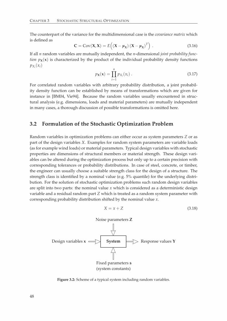
CHAPTER 3 STOCHASTIC STRUCTURAL OPTIMIZATION
The counterpart of the variance for the multidimensional case is the covariance matrix which
is defined as
C = Cov(X, X) = E(
(X − µX) (X − µX)T)
. (3.16)
If all n random variables are mutually independent, the n-dimensional joint probability func-
tion pX(x) is characterized by the product of the individual probability density functions
pXi(xi)
pX(x) =n∏
i=1
pXi(xi) . (3.17)
For correlated random variables with arbitrary probability distribution, a joint probabil-
ity density function can be established by means of transformations which are given for
instance in [BM04, Vie94]. Because the random variables usually encountered in struc-
tural analysis (e.g. dimensions, loads and material parameters) are mutually independent
in many cases, a thorough discussion of possible transformations is omitted here.
3.2 Formulation of the Stochastic Optimization Problem
Random variables in optimization problems can either occur as system parameters Z or as
part of the design variables X. Examples for random system parameters are variable loads
(as for example wind loads) or material parameters. Typical design variables with stochastic
properties are dimensions of structural members or material strength. These design vari-
ables can be altered during the optimization process but only up to a certain precision with
corresponding tolerances or probability distributions. In case of steel, concrete, or timber,
the engineer can usually choose a suitable strength class for the design of a structure. The
strength class is identified by a nominal value (e.g. 5% quantile) for the underlying distri-
bution. For the solution of stochastic optimization problems such random design variables
are split into two parts: the nominal value x which is considered as a deterministic design
variable and a residual random part Z which is treated as a random system parameter with
corresponding probability distribution shifted by the nominal value x.
X = x + Z (3.18)
Design variables x System
Noise parameters Z
Fixed parameters s
(system constants)
Response values Y
Figure 3.2: Scheme of a typical system including random variables.
48

3.2 Formulation of the Stochastic Optimization Problem
z
y
p y( )Y
f z( )
p z( )Zz
y
p y( )Y
p z( )Z
f z( )
Figure 3.3: Influence of a random variable Z with probability distribution pZ(z) on the distribution
pY(y) of a response value Y.
After this decomposition, the system under consideration can be depicted schematically as
in Figure 3.2. The design variables x are exclusively deterministic variables, and all ran-
dom variables (commonly referred to as noise parameters or simply noise) are combined to a
random vector Z. The system constants s noted in the scheme represent all deterministic
parameters that influence the system but are beyond control of the designer.
In optimization problems where noise parameters are present in the formulation of ob-
jective or constraints, Equations (2.6a-d) cannot be applied because the response values for
f , gj, and hk are not deterministic values but also random values Y with corresponding
probability distributions pY(y), as illustrated in Figure 3.3. The figure depicts the case of a
problem with one noise variable Z with the probability density function pZ(z). The distri-
bution pY(y) of the random response value Y is obtained by mapping Z onto the response
by means of the corresponding governing equation. In general, the probability distribution
of the response also depends on the settings of the design variables x. In the case of Fig-
ure 3.3, the governing equation is f (z). In a general optimization problem, objective f , and
constraint functions gj, and hk, respectively, map the random input variables onto random
response values. The shape of the resulting distribution density function pY(y) will strongly
depend on the form of the governing equation.
In order to solve the stochastic optimization problem with its random response values, a
substitute optimization problem must be established in which all response values are deter-
ministic. This is usually done by means of descriptive statistics, which extracts deterministic
quantities from random response values. Many different possibilities exist to transform the
original problem with stochastic response values into an optimization problem with de-
terministic output. Due to their different role in the optimization process, the stochastic
objective function, equality, and inequality constraints are typically replaced by particular
substitute formulations. In the present work, the discussion of possible approaches will be
restricted to commonly used and reasonable formulations.
49

CHAPTER 3 STOCHASTIC STRUCTURAL OPTIMIZATION
3.2.1 Equality Constraints Dependent on Random Variables
As soon as random variables influence the response values for equality constraints hk(x, Z),
the equality hk = 0 cannot be fulfilled for all z ∈ Ω. On this account, equality constraints
should be avoided in the configuration of optimization problems with random variables.
This can be accomplished by substituting the equality requirement into the formulation of
objective and inequality constraints. This approach is proposed for all constitutive equality
constraints such as the equilibrium condition in structural analyses [Das00]. If equality con-
straints depending on random variables cannot be evaded in the problem formulation, they
are in general only fulfilled in a mean sense by substituting Equation (2.6c) by
hk(x) = E(
hk(x, Z))
= 0 . (3.19)
As another apparent alternative, the expected values for the random variables Z can be used
to evaluate the equality constraints
hk(x, Z) = hk
(
x, E(Z))
= 0 . (3.20)
In either case, however, the equality will be violated for most events z ∈ Ω, an inherent and
unavoidable fact related to equality constraints that depend on random variables.
3.2.2 Inequality Constraints Dependent on Random Variables
In stochastic optimization, inequality constraints can be met with 100% probability i.e.
P
gj(x, Z) ≤ 0
= 1 ∀ z ∈ Ω ; j = 1, . . . , ng (3.21)
only in some special cases, for instance if the distributions of all random variables are
bounded. In this case, the feasible design must back off the active constraints by a cer-
tain tolerance such that for all possible events z ∈ Ω the design x is always feasible. Con-
sequently, the worst case of all z ∈ Ω with respect to the constraint functions defines the
feasible domain.
gj(x, Z) ≤ 0 ∀ z ∈ Ω ; j = 1, . . . , ng . (3.22)
For a worst-case design, the probability distribution of the random variables within the
bounds is of no importance, only the tolerance range influences the solution of the opti-
mization problem. Hence, this formulation is often used if only vague (or even no) informa-
tion on the probability distributions involved can be obtained and only tolerance ranges are
dependably available.
In most engineering applications, there is no design x ∈ Rn which meets all constraints
with 100% probability. Thus, each design x will have a finite probability of failure PF, which is
defined by the probability of violating the constraints.
PF = P
gj(x, Z) > 0
∀ z ∈ Ω ; j = 1, . . . , ng (3.23)
Accordingly, the probability of failure can be computed by the integral of the (joint) proba-
bility density function over the infeasible domain U , as illustrated in Figure 3.4.
50

3.2 Formulation of the Stochastic Optimization Problem
z
y
g z( )
p zZ( )
Probability of failure
Figure 3.4: Probability of failure as integral of the probability density function over the infeasible
domain for a 1D problem with one constraint.
P
gj(x, Z) > 0
=
∫
U
pZ(z) dz ; j = 1, . . . , ng (3.24)
with
U = z ∈ Ω | gj(x, Z) > 0 (3.25)
The probability of failure can be used to reformulate the inequality constraints in Equa-
tion (2.6b) as
P
gj(x, Z) > 0
− Pmax ≤ 0 ∀ z ∈ Ω ; j = 1, . . . , ng (3.26)
using an additional optimization parameter Pmax, the maximum allowable probability of
failure. The complement of the probability of failure is the probability of safety (also called
reliability)
PS = P
gj(x, Z) ≤ 0
= 1 − PF ∀ z ∈ Ω ; j = 1, . . . , ng . (3.27)
Derived from the level of reliability that is predefined by the designer, this formulation of
the stochastic optimization problem is commonly termed reliability-based design optimization
(RBDO).
A more general approach to handle constraints subject to noise assigns an individual
cost function γ(y) to the possible violation of each constraint. Hence, the cost function γ(y)
assigns absolute costs to each possible state of the constraint y = g(x, z). In view of the
fact that an increasing violation of the constraint should be related to equal or higher costs,
these cost functions should be monotonically non-decreasing i.e. γ(a) ≤ γ(b) for a < b. The
expected cost for constraint violation can be restricted to a maximum allowable cost Γ by
transforming the condition in Equation (2.6b) into
E(
γj
(
gj(x, Z)))
− Γj ≤ 0 for each j = 1, . . . , ng . (3.28)
If the HEAVISIDE function (depicted in Figure 3.5 and sometimes also referred to as saltus
function)
51

CHAPTER 3 STOCHASTIC STRUCTURAL OPTIMIZATION
g
1
γ( )g
Figure 3.5: HEAVISIDE function.
γ(g) =
0 , g ≤ 0
1 , g > 0(3.29)
is used to represent the costs of each constraint violation, Equation (3.28) turns out to be
equivalent to Equation (3.26).
E(
γ(
gj(x, Z)))
=
∫
Ω
γ(
gj(x, z))
pZ(z) dz =
∫
U
pZ(z) dz = P(
gj(x, Z) > 0)
(3.30)
Each of the proposed approaches to handle inequality constraints in the stochastic optimiza-
tion problem defines a new feasible domain C by means of Equations (3.22), (3.26), or (3.28),
respectively.
3.2.3 Objective Function Dependent on Random Variables
Due to the randomness in Z, the objective function f (x, Z) in Equation (2.6a) must also
be replaced by a deterministic substitute function ρ(x) that provides some representative
value for the random variable Y = f (x, Z) to find a minimum. In stochastic optimization
problems, a design x∗ is considered as optimal if it fulfills the relationship
f (x∗, Z) ≤ f (x, Z) ∀ x ∈ C ∧ z ∈ Ω (3.31)
i.e. if for this design the noise has no deteriorative (increasing) effect on the objective func-
tion and if there is no other design that results in a lower objective for any realization of
z ∈ Ω. A design x∗ that fulfills the relation in Equation (3.31) is called optimal robust design.
Figure 3.6 depicts a function f (x, Z) where the range of possible variations Z around the
design x∗ has no influence on the response y∗ = f (x∗, Z). Under each circumstance z ∈ Ω,
the value for the objective function is always minimal. Accordingly, x∗ is an optimal robust
design.
In the context of stochastic optimization, the term robustness has a distinctive definition:
A system is called robust if the effect of a noisy input on the system response is minimal. This
notion is illustrated in Figure 3.7 where the objective function f is dependent on one random
52

3.2 Formulation of the Stochastic Optimization Problem
x Z*,
x Z,
y
f x Z( , )*
Figure 3.6: Optimal robust design x∗.
design variable X. This design variable is separable in a deterministic part x (the mean of
X) and random variable Z with a normal distribution pZ(z) such that X = x + Z. The mean
of Z is fixed to zero and the variance σ2 is constant i.e. at every setting x, the probability
distribution has the same spread. For each design x, the distribution of the noise pZ(z) is
mapped onto the response by the functional relationship Y = f (X) = f (x + Z) resulting
in a distribution pY(y) for the (random) response Y. In general, this distribution changes in
position and shape dependent on the setting of the design variable. Hence, designs can be
identified that result in a narrow distribution, others yield a larger variation in the response.
Although design x1 yields a lower value for the objective in the deterministic case, design x2
is more robust in presence of noise because the variation of the resulting distribution pY(y)
is smaller. Thus, large deviations from the deterministic (or nominal) case are less likely to
occur.
For most engineering problems, there are no optimal robust designs x∗ ∈ C which mini-
mize f (x, Z) for each possible realization of z ∈ Ω (as for instance in the problem depicted
in Figure 3.7). To identify the best possible approximation is the central problem in statis-
tical decision theory [Fer67, Ber85, Lau05] which provides some effective substitute formu-
lations. Based on the information available for the random variables, two different types of
decision-theoretic approaches are distinguished [JZ72]:
Decisions under risk are made when probability densities for the random input variables Z
are available, and hence, probability distributions pY(y) for the response values can be
obtained.
Decisions under uncertainty subsume cases where only the possible range of each noise
variable is known. About the associated probability density, however, no information
is readily available. As a result, the set of possible output realizations can be deter-
mined but no distribution density can be assigned.
Each substitute formulation gains a scalar value from the originally random output Y of
the objective providing a deterministic measure to assess the merit of each design during
optimization. The proper choice for this so-called robustness criterion ρ is strongly problem
53

CHAPTER 3 STOCHASTIC STRUCTURAL OPTIMIZATION
x1 x2
x
z
y=f x( )
p zZ( )
f x( )
y
p yY( )
Figure 3.7: Robust vs. non-robust settings for a 1D problem with one random design variable X.
dependent and essentially an engineering decision. It should be noted that all formulations
represent an approximation to the desired optimal robust case, and hence, imply some kind
of compromise loosening the condition in Equation (3.31).
Example 2. To illustrate the different approaches and to facilitate a direct comparison, this
example is used repeatedly for each robustness criterion. The objective function (see Fig-
ure 3.8)
f (x, z) = (2 − x) (0.1 − z − 0.1 x) + 0.3
for this example depends on one (deterministic) design variable x and one noise variable Z.
The discussion of commonly applied robustness criteria is started with decisions under
uncertainty:
Minimax principle. For some optimization tasks, a worst case scenario could be of interest,
which requires the random response to be bounded on Ω. In this case, the deterministic
substitute formulation ρ(x) for the stochastic objective function f (x, Z) reads
ρ(x) = supz∈Ω
f (x, z) . (3.32)
This formulation is also called minimax principle [vN28, Wal50]. For each setting of design
variables x, the effects of all possible events z ∈ Ω are scanned, and the outcome for the
worst case is taken as decisive gage to assess the robustness of the current design. This
54

3.2 Formulation of the Stochastic Optimization Problem
Figure 3.8: Objective function for Example 2 with one design variable x and one noise variable Z.
approach is also referred to as maximin principle for cases where the optimization problem is
formulated as maximization task.
The minimax principle ignores the possible range in the output. Instead, it identifies the
upper limit of the resulting range, and hence, it caps the deteriorative effects of the noise
parameters. This robustness criterion leads to very conservative designs as it is based upon
an extremely pessimistic attitude.
Example 2 [continued]. For the “decision under uncertainty” criteria, assume that the dis-
tribution of noise variable Z is unknown and only prescribed tolerances ±0.2 delimit Z.
Based on this assumption, the minimax principle in Equation (3.32) is applied to the above
introduced example.
Figure 3.9 depicts a projection of the objective function onto the x-y plane. Hence, it
shows the possible range of output realizations for each x and z ∈ [−0.2, 0.2]. The minimax
principle allocates the upper limit of this range for each x as robustness criterion yielding the
deterministic substitute function ρ(x) depicted in Figure 3.10. The minimum of ρ(x), which
represents the optimal setting for the design variable resulting from the minimax principle,
is located at x∗ = 2.0.
Minimax regret criterion. The minimax regret criterion focuses on minimizing the maxi-
mum regret that may result from making non-optimal decisions i.e. choosing a non-optimal
design x. SAVAGE [Sav51] and NIEHANS [Nie48] define regret as opportunity loss to the deci-
sion maker if design x is chosen and event z ∈ Ω happens to occur. The opportunity loss is
55

CHAPTER 3 STOCHASTIC STRUCTURAL OPTIMIZATION
x0
1 2 3 4
y
0.2
0.4
0.6
0.8
1
1.2
Figure 3.9: Projection of the objective function onto x-y plane.
ρ x( )
x
Figure 3.10: Surrogate function ρ(x) resulting from Figure 3.8 for minimax principle.
the difference in the objective between the best obtainable response f ∗
f ∗(z) = infx∈C
f (x, z) (3.33)
for each possible event z and the actual outcome f (x, z) resulting from choosing x
ρ(x) = supz∈Ω
(
f (x, z) − f ∗(z))
. (3.34)
To obtain f ∗(z), all possible events are investigated separately, and the optimal decision x∗
for each z ∈ Ω is evaluated assuming the underlying event occurs uniquely.
Another view at the minimax regret criterion would be that first, the best achievable
response value for each event z is subtracted from f (x, z), then the worst case is determined
as for the minimax criterion. As a result, the optimal design is identified as the one for
which the worst case has a minimal deviation from the theoretical optimum f ∗. Hence, the
minimax regret criterion also takes into account the range of possible response values as
opposed to the original minimax principle.
56

3.2 Formulation of the Stochastic Optimization Problem
z
y
f x,z( )
f z*( )
0
0.2
0.2 0.1 – 0.1 – 0.2
0.4
0.6
0.8
1
1.2
Figure 3.11: Projection of the objective function onto z-y plane.
x
ρ x( )
Figure 3.12: Surrogate function ρ(x) resulting from Figure 3.8 for minimax regret criterion.
Example 2 [continued]. Referring to the assumption z ∈ [−0.2, 0.2], the minimax regret
criterion in Equation (3.34) can be evaluated for the established example. To find f ∗(z), the
objective function is projected onto the z-y plane as depicted in Figure 3.11. The lower bound
of the span (dashed line in Figure 3.11) represents f ∗(z). With f ∗(z), the opportunity loss
f (x, z) − f ∗(z) is determined for each combination of decision x and event z. The minimax
principle applied to the opportunity loss results in the deterministic substitute function ρ(x)
depicted in Figure 3.12. The optimal design characterized by this minimax regret criterion
is located at x∗ = 1.5.
LAPLACE method. LAPLACE argues that for a serious assessment of a stochastic problem,
the designer should allot a probability distribution pZ(Z) to the noise. In absence of estab-
lished probability information for the noise, he suggests the use of the principle of insufficient
reason by BERNOULLI. It states that, if no probabilities have been assigned, there is insuf-
57

CHAPTER 3 STOCHASTIC STRUCTURAL OPTIMIZATION
ficient reason to indicate that any state for Z is more or less likely to occur than any other
state. Consequently, all events must be equally likely. Accordingly, a uniform distribution is
assigned to the noise variables. This assumption turns the problem into a “decision under
risk” problem. In this case, the assumed probability density function for the input allows
for an estimation of the output distribution.
With information about the distribution of the random response at hand – either based
on BERNOULLI’s argument or derived from probability distributions known in advance –
more detailed robustness criteria for the class of “decision under risk” problems can be for-
mulated. The question on how to find this distribution of the response when the probability
density of the noise parameters is known will be discussed in Section 3.3.
Quantile measures. Based on the probability density distribution of the output, a quantile
q (e.g. 90% quantile) of the random objective function can be used as robustness criterion in
analogy to the worst case.
ρ(x) = C−1(x, q) (3.35)
where C−1 denotes the inverse of the cumulative distribution function for the random ob-
jective Y = f (x, Z) as introduced in Equation (3.7). Here, C−1 is also a function of the design
variables x because generally the probability density pY of the response also depends on the
design variables.
For the resulting robust design x∗, the respective percentage of possible realizations z ∈Ω will yield a value for the objective f (x∗, Z) that is equal to or smaller than ρ(x∗). Similar
to the worst case formulation, the quantile measure disregards the possible spread in the
random response.
Example 2 [continued]. For the evaluation of “decision under risk” criteria, a probability
distribution pZ(z) for the noise variable Z has to be specified. To illustrate the impact of the
probability distribution on the resulting optimal design, two different cases are studied for
this example:
⋄ a uniform distribution according to Equation (3.12) with aZ = −0.2 and bZ = 0.2 and
⋄ a normal distribution as defined in Equation (3.11) with µZ = 0.02 and σZ = 0.05
as depicted in Figure 3.13.
Evaluating Equation (3.35) based on the aforementioned probability distributions for the
noise variable Z and a 90% quantile results in the plots in Figure 3.14. The minimum for this
criterion is located at x∗unif = 1.9 and x∗norm = 1.72 for the uniform distribution and the
normal distribution, respectively.
If this criterion is evaluated for q = 1, the resulting substitute function ρ(x) for the uni-
form distribution is equal to the minimax principle. For the normal distribution, no substi-
tute function can be determined since the resulting distribution is essentially not bounded.
Hence, the criterion yields infinite values for ρ(x).
58

3.2 Formulation of the Stochastic Optimization Problem
z
Normal distribution
Uniform distribution
0
2
4
6
8
0.20.1– 0.1– 0.2
Figure 3.13: Probability distributions pZ(z) assumed for noise variable Z in Example 2.
x0
1 2 3 4
0.2
0.4
0.6
0.8
1
1.2
Normal distribution
Uniform distribution
ρ x( )
Figure 3.14: Surrogate functions ρ(x) based on the quantile criterion with q = 0.9 applied to Exam-
ple 2.
BAYES principle. For this criterion, the expected value for the random response Y =
f (x, Z) is evaluated.
ρ(x) = E(
f (x, Z))
= µY(x) =
∫
Ω
f (x, z) pZ(z) dz (3.36)
Example 2 [continued]. The definition in Equation (3.36) constitutes the plots in Fig-
ure 3.15. The minimum mean value for the objective is obtained for designs x∗unif = 1.5
and x∗norm = 1.4, respectively.
In general, taking into account only the mean value of the objective can result in a non-
robust design because it disregards the spread of the distribution. In other words, this crite-
rion makes no difference between a narrow response distribution pY(y) and a wide spread
59

CHAPTER 3 STOCHASTIC STRUCTURAL OPTIMIZATION
x0
1 2 3 4
0.2
0.4
0.6
0.8
1
1.2
Normal distribution
Uniform distribution
ρ x( )
Figure 3.15: Surrogate functions ρ(x) based on the BAYES principle applied to Example 2.
p yY( )0
10 20 30 40
y
0.2
0.4
0.6
0.8
1
1.2
Figure 3.16: Probability distributions pY(y) with identical mean but unequal standard deviation.
distribution if both have the same mean value as exemplified in Figure 3.16. Hence, the
average performance of the design will be optimal but at the price of possibly large deviations
from the mean performance. Consequently, the BAYES principle is used in cases where the
good prospects of “beneficial deviations” due to noise balance the risks of “deteriorating
effects” of noise variables. In many engineering problems, this approach is not appropriate,
for instance a typical manufacturing process: beneficial deviations from the average perfor-
mance of the product usually do not generate higher profit for the individual item whereas
inferior goods surely entail additional costs for quality control and repair. In decision theory,
a distinction is drawn between three different situations or attitudes:
1. A decision maker that places more emphasis on the chances of beneficial deviations.
His behavior is called risk-taking.
2. A decision maker that ascribes equal weights to positive and negative deviations. His
behavior is called risk-neutral.
60

3.2 Formulation of the Stochastic Optimization Problem
3. A decision maker that lays stress on the deteriorative effects of variations. His behav-
ior is called risk-averse.
In comparison with the BAYES principle – the preferred strategy for the risk-neutral de-
signer – the substitute function of a risk-taker is smaller where significant variance exists.
The risk-averse designer will augment the substitute function in comparison to the mean
wherever the variance is large. The latter strategy leads to substitute functions ρ(x) for ro-
bust design optimization that yield robust designs in terms of the above given definition –
optimizing the overall performance while minimizing the variation due to noise.
Robustness criteria based on location and dispersion measures. Although all of the
aforementioned strategies surely have their suitable applications, a minimal variation in
the system performance proves to be beneficial for most stochastic optimization problems
in structural engineering. In these cases, a multicriteria optimization with two objectives is
necessary to characterize the optimum: to minimize the location and the dispersion of the
random response, for instance the mean and the variance. As described in Section 2.1.4,
several techniques are available to solve this multiobjective optimization problem.
If the composite function approach is used as introduced in Equation (2.2), the two ob-
jectives are combined to one robustness criterion by a weighted sum with user-specified
weighting factors w1 and w2. Since the location of extrema does not change if a function is
multiplied by a scalar (e.g. 1/w1), one weighting factor can be eliminated without changing
the resulting optimum design (the response value at the optimum, however, is modified by
this scalar multiplication). Here, the weighting factor for the mean is always fixed to 1.0
making the average performance of the system the gage which is adjusted by a multiple
(weight w) of the dispersion measure. Hence, the response values of the resulting substi-
tute functions have a plain meaning potentiating a straightforward comparison of different
“robustness measures”. In terms of decision theory, w = 0 corresponds to a risk-neutral
designer, w < 0 describes the preference of a risk-taker, and w > 0 expresses risk-aversion.
For the aim of robust design optimization (identifying a design x with minimal variance in
the response) only values w > 0 make sense.
ρ(x) = E(
f (x, Z))
+ w V(
f (x, Z))
= µY(x) + w(
σY(x))2
= µY(x) + w
∫
Ω
(
f (x, z) − µY(x))2
pZ(z) dz .
(3.37)
To solve engineering problems, it is often more suitable to constitute the robustness criterion
using the standard deviation instead of the variance. As a result, both the measure of central
tendency and measure of dispersion and hence the resulting robustness criterion have the
same unit as the original objective function.
ρ(x) = E(
f (x, Z))
+ w√
V(
f (x, Z))
= µY(x) + w σY(x)
(3.38)
61

CHAPTER 3 STOCHASTIC STRUCTURAL OPTIMIZATION
The signal to noise ratio (SNR) as introduced by TAGUCHI [FC95] is also a robustness cri-
terion based on the mean and the variance of a system response Y. Considering the case the
smaller – the better, TAGUCHI assumed zero as the minimal possible response value. Accord-
ingly, he formulated the following SNR as robustness criterion
SNR = 10 log10
(
µ2Y + σ2
Y
)
. (3.39)
Since TAGUCHI performed a maximization of the SNR to find the optimum, his formulation
of the SNR has the opposite sign. The operator “10 log10” does not change the location of the
optimum, it simply transforms the magnitude of the robustness criterion into decibel units
(dB). To make this robustness measure comparable to ρ(x) in Equations (3.32) – (3.38), the
SNR is altered as follows
ρ(x) =(
µY(x))2
+(
σY(x))2
=(
µY(x))2
+
∫
Ω
(
f (x, z) − µY(x))2
pZ(z) dz
=(
µY(x))2
+
∫
Ω
( f (x, z))2 pZ(z) dz −(
µY(x))2
=
∫
Ω
( f (x, z))2 pZ(z) dz = E(
(
f (x, Z))2)
.
(3.40)
Since a monotonic transformation of a function does not change the position of its extrema
but only the absolute value of the function (as the transformation 10 log10 above), such a
transformation can be applied to ρ(x). For a positive argument (·), the positive root√·
is a monotonic transformation. After taking the positive root of the formulation in Equa-
tion (3.40), the resulting robustness criterion has the same unit as the original objective func-
tion. Additionally, a weighting parameter w is introduced to allow for individual emphasis
on the minimization of variations.
ρ(x) =
√
(
µY(x))2
+(
w σY(x))2
(3.41)
To compare the robustness criteria in Equations (3.37), (3.38), and Equation (3.41), so-called
indifference curves are introduced. Originally developed for decision making in operations
research, indifference curves are in fact contour lines of a function Ψ(µ, σ) combining the
two objectives “mean” and “standard deviation” to one objective function. Each contour
marks all combinations of µ and σ that the decision maker would equate in his personal
preference i.e. between these µ-σ pairs, the decision maker is indifferent.
For a risk-neutral decision maker, the indifference curves are always parallel to the σ-
axis. If a risk-averse criterion is chosen, the indifference curves are strictly decreasing with
µ (∂σ/∂µ < 0) while for risk-takers they are strictly increasing (∂σ/∂µ > 0) as illustrated in
Figure 3.17. Since in most operations research texts the aim of the optimization is the max-
imization of the original objective function, the assignments of positive and negative slope
in the indifference curves to risk-taker and risk-averse decision maker are interchanged.
62

3.2 Formulation of the Stochastic Optimization Problem
μ
σ
μ
σ
μ
σ
Risk-taking Risk-neutral Risk-averse
Ψ−
Ψ−
Ψ−
Figure 3.17: Indifference curves dependent on the attitude of the decision maker.
μ
σ
1
1
02
2
3
3
4
4
const.22 =+=Ψ σμ
μ
σ
1
1
02
2
3
3
4
4
const.=+=Ψ σμ
μ
σ
1
1
02
2
3
3
4
4
const.2 =+=Ψ σμ
Figure 3.18: Indifference curves for robustness criteria in Equations (3.37), (3.38), and (3.41).
Based on the graphs in Figure 3.18 displaying Equations (3.37), (3.38), and (3.41) with
w = 1, the difference between these robustness criteria can be evaluated. Compared to ρ(x)
in Equation (3.38), the robustness criterion in Equation (3.37) only slightly penalizes small
standard deviations (σ ≪ 1). This means that for exiguous variations (σ → 0), the decision
maker behaves almost risk-neutral (∂σ/∂µ → −∞). In contrast, large standard deviations
are severely penalized.
A special trait of Equation (3.41) is that with increasing mean the same standard devia-
tion is regarded as less critical. For constant σ and increasing µ the slope of the indifference
curves steepens. This can be useful in cases where the designer’s assessment of variation
is not fixed but relative to the absolute value of the mean. The main limitation of this for-
mulation is that the mean value is restricted to be larger than or equal to zero by definition.
Thus, this criterion can only be used if the objective function f (x, Z) cannot result in negative
values.
Based on the definition of indifference curves, the decision maker may additionally es-
tablish different functions Ψ(σ, µ) and thus custom-made robustness criteria to account for
an individual rating of different (µ, σ) pairs.
Example 2 [continued]. To illustrate the results of the composite function approach, the
shape of the two components must be introduced first. The mean µY(x) was introduced
earlier and is depicted in Figure 3.15. The standard deviation σY(x) for both probability
63

CHAPTER 3 STOCHASTIC STRUCTURAL OPTIMIZATION
x0
1 2 3 4
σY
0.1
0.2 Normal distribution
Uniform distribution
Figure 3.19: Standard deviation σY of the resulting probability density pY(y) for Example 2.
x0
1 2 3 4
0.2
0.4
0.6
0.8
1
1.2
Normal distribution
Uniform distribution
w = 1
w = 3
ρ x( )
Figure 3.20: Surrogate functions ρ(x) for composite robustness criterion in Equation (3.37) with var-
ied weighting factor w.
distributions of this example is shown in Figure 3.19. Evaluating Equation (3.37) by choos-
ing w = 1 and w = 3 yields the substitute functions depicted in Figure 3.20. Compared to
the substitute function solely based on the mean, the composite function approach results
in designs with lower variation in the response. For w = 1, the minima are represented
by x∗unif = 1.559 and x∗norm = 1.415, respectively. If the designer’s emphasis is on designs
with lower variation in the objective, this intention can be expressed by increasing w. Ac-
cordingly, the optimum is shifted toward the minimum of the variance (located at x = 2).
Choosing w = 3 for instance, relocates the minima to x∗unif = 1.643 and x∗norm = 1.442,
respectively.
Figure 3.21 contains the graphs resulting from Equation (3.38). The optimal designs
based on this robustness criterion with w = 1 are found at x∗unif = 2 and x∗norm = 1.65,
respectively. Considering the case w = 3, the optimum for the uniform distribution remains
unchanged because the standard deviation at x = 2 is equal to zero. Thus, a higher penalty
factor on σ does not influence the optimum. For the normal distribution, the optimum is
moved to the minimum in the standard deviation, thus constituting the minimum for w = 3
64

3.2 Formulation of the Stochastic Optimization Problem
x0
1 2 3 4
0.2
0.4
0.6
0.8
1
1.2
Normal distribution
Uniform distribution
w = 1
w = 3
ρ x( )
Figure 3.21: Surrogate functions ρ(x) for composite robustness criterion in Equation (3.38) with var-
ied weighting factor w.
x0
1 2 3 4
0.2
0.4
0.6
0.8
1
1.2
w = 1
w = 3
Normal distribution
Uniform distribution
ρ x( )
Figure 3.22: Surrogate functions ρ(x) for composite robustness criterion in Equation (3.41) with var-
ied weighting factor w.
at x∗norm = 2.
The robustness criterion formulated in Equation (3.41) is also evaluated for the two al-
ternative distribution functions and both weighting factor settings w = 1 and w = 3. In
Figure 3.22, the corresponding substitute functions are plotted and the resulting optimal
designs are indicated at x∗unif = 1.597 and x∗norm = 1.427 for w = 1, and x∗unif = 1.838 and
x∗norm = 1.578 for w = 3, respectively.
As an alternative solution procedure for the multicriteria optimization involving both
mean and standard deviation as objective functions, the preference function approach can be
applied as well. In this case, either component can be chosen as preference function (the
actual objective function) while the other part is transformed into an additional constraint by
imposing a maximum permissible value (σmax or µmax) on the respective quantity. According
to Equation (2.1), the substitute formulation for the stochastic optimization problem then
65

CHAPTER 3 STOCHASTIC STRUCTURAL OPTIMIZATION
x0
4
y
F x( )
g x( )0.2
– 0.2
0.4
0.6
0.8
1
1.2
1 2 3
Feasible
domain
Figure 3.23: Robust design based on the preference function approach with upper limit on the stan-
dard deviation σmax = 0.02.
reads
F(x) = µY(x) (3.42)
g(x) = σY(x) − σmax ≤ 0 ,
or alternatively,
F(x) = σY(x) (3.43)
g(x) = µY(x) − µmax ≤ 0 .
Formulation (3.42) is used if the aim of the optimization is in fact not to obtain a “true”
robust design (with minimal variance) but a design with optimal average performance for
which the variance in the performance is not larger than a prescribed tolerance value σmax.
The second approach might be the proper choice in cases where an optimization based on
nominal values already exposed a design that would perform optimal in the deterministic
case. Following the concept of Equation (3.43) would then allow to “back off” this theoretical
optimum by a certain acceptable loss in average performance to minimize the variance due
to the noise.
Example 2 [continued]. As an example for the preference function approach, emphasis
is put on minimization of µY(x), which is henceforth the actual objective F(x). For the
standard deviation σY(x), an upper bound is established by setting σmax = 0.02. Thus, the
objective to minimize the variance is transformed into a constraint g(x) = σY(x) − 0.02. In
Figure 3.23, the new constraint g(x) is plotted assuming the noise is normally distributed.
Minimizing the preference function F(x) = µY(x) on the feasible domain characterized by
g(x) ≤ 0 yields the optimal design at x∗norm = 1.605.
Cost function. Similar to the procedure for inequality constraints, cost functions γ(y) can
be introduced to find a substitute formulation ρ(x) for robust design optimization. Since
66

3.2 Formulation of the Stochastic Optimization Problem
x0
1 2 3 4
50
100
150
200
250
300
ρ x( )
Normal distribution
Uniform distribution
Figure 3.24: Robust design based on the cost function approach for Example 2.
particular costs are related to each possible response value y of f (x, z) and y = g(x, z),
the expected overall costs for violation of constraints and variation in the objective can be
optimized.
ρ(x) = E (γ0 ( f (x, Z))) +
ng∑
j=1
E(
γj
(
gj(x, Z)))
=
∫
Ω
γ0 ( f (x, Z)) pZ(z) dz +
ng∑
j=1
∫
Ω
γj
(
gj(x, Z))
pZ(z) dz
(3.44)
The advantage of the cost function approach is that the trade-off between the different ele-
ments of the stochastic optimization problem (violation of each constraint, mean and vari-
ance of the objective) is judged on a consistent basis, namely the individual cost (e.g. in
terms of money or alternative measures such as the weight) contributed by each element of
the optimization formulation. At the same time, the problem usually becomes an uncon-
strained optimization problem since all constraints are expressed in terms of their monetary
equivalent and are summarized in the new objective function, the overall costs. The prob-
lem with this approach is to define appropriate and accurate cost functions for each possible
contribution.
Example 2 [continued]. The quadratic cost function
γ0(y) = 300 y2 + 60 y
is supposed to describe the costs associated with a design x that produces the outcome
y = f (x). Since no constraints are formulated for this example, only the first expression in
Equation (3.44) contributes to the substitute function ρ(x). Figure 3.24 shows the evaluation
of Equation (3.44) for the two probability density functions under investigation. The optimal
designs based on minimum expected costs are x∗unif = 1.420 and x∗norm = 1.575, respectively.
67

CHAPTER 3 STOCHASTIC STRUCTURAL OPTIMIZATION
Concluding the Discussion of Introduced Robustness Criteria. A look at the substitute
formulations applied to Example 2 reveals that each robustness criterion yields a distinct
“robust design”. It should be realized that for each formulation an engineering problem can
be conceived which justifies and substantiates the eligibility of the corresponding criterion
as an approximation to the (in most cases) unattainable goal of an optimal robust design.
In general, one optimization problem can successfully be tackled via miscellaneous robust-
ness criteria. For all intents and purposes, there is no better or worse robustness criterion;
the proper choice for a suitable formulation is basically an engineer’s decision. In fact, this
conclusion was already suggested earlier by introducing decision-theoretic methods where
the different criteria were derived depending on the preference of the decision maker. The
individual choice should be made based on available information on the noise (probability
density function or range) and the designer’s demand on the system performance (main
focus on good overall performance or more emphasis on minimal variance). Moreover, as
revealed by the discussion of multicriteria optimization problems in Section 2.1.4, problems
with more than one objective (in this case: location and dispersion of the probability dis-
tribution pY) do not have a unique solution but bring up a set of PARETO-optimal designs
from which the designer has to pick his personal favorite.
3.2.4 Stochastic Optimization Terminology: Robustness versus Reliability
Many examples for stochastic optimization problems are described in the literature but,
unfortunately, they are not always termed coherently. In this text, a consistent terminology
is proposed that tries to combine the established terms from different communities.
Before the field of stochastic optimization can be addressed, stochastic optimization proce-
dures and stochastic optimization problems must be distinguished. The first term summarizes
all optimization algorithms that use stochastic sampling to find the solution of an optimiza-
tion problem, for instance random search or evolutionary algorithms. The problem to be
solved – as defined in Equations (2.6a-d) – does not have to be a stochastic optimization
problem. Stochastic optimization procedures are also successfully applied to determinis-
tic optimization problems i.e. where all parameters and variables involved are inherently
deterministic. Correspondingly, stochastic optimization problem as a generic term subsumes
the analysis of problems which comprise random variables in the problem formulation. To
solve a stochastic optimization problem, it is not mandatory to choose a stochastic optimiza-
tion procedure. Other solution techniques (as introduced in Section 2.3) can also be applied
to this class of problems using substitute formulations presented earlier.
In many texts, the terms robust design (or robustness) problem and reliability problem are
used to denote stochastic optimization problems. The matter which is actually labeled by
these expressions, though, differs from author to author. Frequently, the entire field of prob-
lems with random variables is called “robust design optimization” [LP01, JL02]. In this
text, any problem formulation containing functions of random variables is called a general
stochastic optimization problem. Moreover, two special cases are distinguished depending on
the functions affected by variations: objective function or constraints. If the objective is
solely a function of deterministic variables and exclusively (inequality) constraints are af-
fected by the random variables, one possible deterministic substitute formulation for this
68

3.3 Methods to Solve Stochastic Optimization Problems
problem reads
minimize f (x) ; x ∈ Rn (3.45a)
such that P
gj(x, Z) > 0
− Pmax ≤ 0 ; z ∈ Ω ; j = 1, . . . , ng (3.45b)
xLi ≤ xi ≤ xU
i ; i = 1, . . . , n . (3.45c)
The problem described by Equations (3.45a-c) is called a reliability problem. In other publi-
cations [PSP93, DC00], the term feasibility robustness is used to describe this problem. The
methods used to solve reliability problems are summarized in the term reliability-based design
optimization (RBDO).
In case the noise variables merely affect the objective function f (x, Z) (i.e. the constraints
are deterministic or the problem is unconstrained), the problem is called a robustness problem
or robust design problem. To solve this optimization task, the original stochastic problem is
transformed into a deterministic form by applying a suitable robustness criterion ρ(x) as
described in Section 3.2.3. The solution of problems according to Equations (3.46a-d) is
termed robust design optimization.
minimize ρ(x) ; x ∈ Rn (3.46a)
such that gj(x) ≤ 0 ; j = 1, . . . , ng (3.46b)
hk(x) = 0 ; k = 1, . . . , nh (3.46c)
xLi ≤ xi ≤ xU
i ; i = 1, . . . , n (3.46d)
This differentiation of the two special cases makes sense with respect to the methods needed
to solve problems of each respective class. In robust design optimization, the mean and
the variance play the most important roles in the formulation of the substitute function
ρ(x). To evaluate mean and variance adequately, a good representation of the probability
distribution in areas with large probability is usually sufficient (e.g. the distribution in the
area µ ± 2 σ). On the other hand, to determine the relevant probability of failure (commonly
Pf ≪ 1‰ is chosen) in reliability problems, the “outer legs” (with low probabilities) of the
probability density must be described accurately (often up to ±6 σ or more) [RB05]. Hence,
the methods used to ascertain the resulting probability density pY by mapping the input
density functions pZ onto the response should accommodate the regions of main emphasis
and their different accuracy requirements.
3.3 Methods to Solve Stochastic Optimization Problems
To solve stochastic optimization problems, the effect of randomness in input parameters on
the crucial response values must be determined. Dependent on the substitute formulation
transforming the stochastic problem into a deterministic form, the evaluation of the objective
and/or constraints for one design involves
⋄ a complete optimization run e.g. to determine the corresponding worst case,
⋄ the calculation of the probability of failure PF for reliability problems,
69

CHAPTER 3 STOCHASTIC STRUCTURAL OPTIMIZATION
⋄ the evaluation of integrals over the probability distribution pY to determine the ex-
pected value and the variance of the crucial response value for the robustness prob-
lem.
For both the minimax principle and the minimax regret principle, an optimization has to
be performed to identify the worst case. Suitable optimization algorithms for different kinds
of problems have been proposed and discussed in Section 2.3. An alternative approach to
determine the robustness criterion ρ for these formulations is to examine only the vertices of
the noise space assuming that the worst case will result from some extremal settings of the
noise variables. This assumption typically holds whenever the effect of the noise variables
is approximately linear, but not in general. Thus, applicability of this simplification should
be examined carefully.
Suitable methods to determine the probability of failure as a prerequisite for reliability
problems comprise
⋄ First-order second moment approach (FOSM)
⋄ First-order reliability method (FORM)
⋄ Second-order reliability method (SORM)
⋄ Monte Carlo sampling (MC)
⋄ Importance sampling (IS)
⋄ Directional sampling (DS)
and many other variants of sampling methods. Since the main issue of this work is rather
to solve robustness than reliability problems, a presentation of methods which are specif-
ically designed to estimate small probabilities will be omitted here. As a consequence
of the large number of publications in this field, a list of references for reliability prob-
lems and solution techniques must be incomplete. The following list is meant to provide
an excerpt of interesting contributions and reviews [TCB82, HR84, SBBO89, GS97, Roo02,
RDKP01, OF02, Sav02, PG02, BM04]. A detailed review of reliability-based optimization
techniques and applications is given in [FM03]. Illustrative examples for reliability prob-
lems and the successful application of the aforementioned techniques can be found e.g.
in [TCM86, LYR02, GFO02, MF03, AM04, YCYG04].
In the following, several techniques to solve the robust design problem will be discussed.
The aim of these approaches is either to find the probability distribution of the output vari-
able pY or to compute directly its statistical measures (mean µY, variance σ2Y). The resulting
data are used as input for the robustness criterion which defines a deterministic substitute
for the original problem.
As already derived in Equations (3.36), (3.37), and (3.40), substitute formulations that are
based on mean and variance of the response involve the evaluation of integrals of the form∫
Ω
κ(z) pZ(z) dz . (3.47)
70

3.3 Methods to Solve Stochastic Optimization Problems
To compute the mean µY(x), the function κ takes the form f (x, z). For the calculation of the
variance σ2Y(x), κ either reads ( f (x, z))2 or ( f (x, z) − µY(x))2 as derived in Equations (3.37)
and (3.40). Since integration is only performed with respect to the noise variables Z, depen-
dency on x can be disregarded for the evaluation of the integral.
In most engineering applications, the functions f , g, and h are not known explicitly.
Typically, the response values y can only be obtained pointwise as solution of a linear system
of equations, for instance by means of the finite element method [ZT05]. Consequently, the
integration has to be performed numerically. For the numerical computation of an integral,
the basic idea is to approximate the original integrand by a function that is easy to integrate.∫
f (z) dz ≈∫
f (z) dz (3.48)
These approximations are constructed by interpolating polynomials which are based on
evaluations of the integrand at m sampling points. With prior knowledge about the class
of polynomials to be used as approximation, the integration can be performed analytically
yielding a weighted sum over the function evaluations at the sampling points.
∫
f (z) dz ≈∫
f (z) dz =m∑
l=1
wl f (zl) (3.49)
The individual weights wi have to be determined according to the class of polynomials used
as approximation and the location of the sampling points. If these sampling points are
equally-spaced, the resulting integration rules are called NEWTON-COTES formulas. A NEW-
TON-COTES formula can be constructed for any polynomial degree. The commonly used
formulas of low degree are known by the names rectangle rule for constant approximations,
trapezoidal rule for linear polynomials, and SIMPSON’s rule for quadratic polynomials. To as-
sure a good accuracy for the NEWTON-COTES formulas, the distance between the sampling
points used for the integration needs to be small. For this reason, numerical integration is
usually performed by splitting the original integration domain Ω into smaller subintervals,
applying a NEWTON-COTES rule on each subdomain, and adding up the results. This pro-
cedure is called composite rule. A similar concept is used by the Gaussian quadrature rule. It
is constructed to yield an exact result for polynomials of degree 2 m − 1 by a suitable choice
of the m points and corresponding weights.
The quadrature rules discussed above are all designed to evaluate one-dimensional in-
tegrals. To compute the mean of response values that depend on multiple noise variables,
multi-dimensional integrals have to be evaluated. One possibility to solve this problem is
to formulate the multiple integral as nested one-dimensional integrals referring to FUBINI’s
theorem. This theorem necessitates some additional assumptions and reads∫
Ω
f (z) dz =
∫
Ω1×Ω2×···×Ωn
f (z) dz =
∫
Ω1
∫
Ω2
· · ·∫
Ωn
f (z) dzn · · · dz2 dz1 . (3.50)
This approach requires the function evaluations to grow exponentially as the number
of dimensions increases. Additionally, it only covers integration over a multi-dimen-
sional domain Ω that can be written as Cartesian product of one-dimensional domains
Ω1 × Ω2 × · · · × Ωn.
71

CHAPTER 3 STOCHASTIC STRUCTURAL OPTIMIZATION
Monte Carlo methods offer an alternative approach to compute multi-dimensional inte-
grals. They may yield greater accuracy for the same number of function evaluations than
repeated integrations using one-dimensional methods.
3.3.1 Plain Monte Carlo Method
Monte Carlo methods make use of the special form of the integral in Equation (3.47). This
integral is solved based on m sampling points which are chosen with respect to the proba-
bility density of the noise variables pZ. After the function κ is evaluated at these sampling
points, the solution of the integral can be approximated by
∫
Ω
κ(z) pZ(z) dz ≈m∑
l=1
wl κ(zl) . (3.51)
In plain Monte Carlo simulations, the sampling points are determined randomly in con-
sistency with the probability density of the noise variables pZ. In consequence of the ran-
dom sampling which is performed according to the probability distribution, the sampled
response values are all weighted equally. In addition, the sum over all weights should add
up to one in accordance with Equations (3.3) and (3.6), respectively.
m∑
l=1
wl = 1 ∧ wl = const. ⇒ wl =1
m(3.52)
As an aside, this approach results in the equation for the sample mean. This formula is
commonly used in descriptive statistics to estimate the mean of a random variable Y whose
distribution pY is not known explicitly. Typically, the characteristics of a random variable
can only be studied by means of sampling. In this case, the sample mean y provides an
estimate for the mean µY based on m random samples yl .
µY ≈ y =1
m
m∑
l=1
yl (3.53)
Analogously, the sample variance s2 is defined as an estimate for the variance of the under-
lying distribution. In minor inconsistency with Equation (3.52), it can be shown that for the
sample variance choosing wl = 1/(m − 1) yields an unbiased estimate for the variance σ2Y.
σ2Y ≈ s2 =
1
m − 1
m∑
l=1
(yl − y)2 . (3.54)
3.3.2 Stratified Monte Carlo Method
By using random sampling, the allocation of sampling points is unsystematic and chances
are that important subsets of the noise space are not taken into account. Especially, if there
are regions with small probability but high impact on the investigated statistics, this influ-
ence might be ignored.
72

3.3 Methods to Solve Stochastic Optimization Problems
Stratified Monte Carlo sampling uses a partitioning of the entire noise space into disjoint
subregions Ωl , so-called strata, to ensure that from each subset samples are included. Typi-
cally, one sample is taken at random from each stratum and so the sample size m is equal to
the number of strata. The weight, that is assigned to each particular sample, is given by the
probability of the corresponding stratum.
wl = Pz ∈ Ωl =
∫
Ωl
pZ(z) dz (3.55)
The strata are often – but not necessarily – selected to have equal probability. Accordingly, in
stratified Monte Carlo, the individual samples can have different weights. If more than one
sample is located in one stratum, the corresponding probability is divided by the number of
samples per stratum to obtain their respective weight. Once the weights wl and the response
values yl have been computed, Equation (3.52) can be used to compute mean and variance
of the investigated random response Y.
Example 3. In this example, a stratified Monte Carlo sampling for eight sampling points
in two dimensions is performed. Random variable Z1 is normally distributed and Z2 varies
according to a uniform distribution as depicted in Figure 3.25. Despite the uniform distribu-
tion of Z2, it is assumed that response values resulting from larger z2 have to be examined
more closely (e.g. because of a highly nonlinear behavior). Accordingly, the strata are cho-
sen to emphasize sampling of the corresponding subregion. By contrast, the range of Z1
is segmented into intervals of equal probability. Clearly, the weights of samples from the
upper row of strata in Figure 3.25 have to be smaller than those from the lower row to avoid
an erroneous evaluation of Equation (3.52).
The big advantage of using stratified Monte Carlo is that the inclusion of specified sub-
regions can be enforced. But then, two major questions have to be answered: how to define
Subregion of
particular importance
z2
z1
Stratum
Figure 3.25: Stratified Monte Carlo sampling for a two-dimensional space with eight strata and one
sampling point per stratum.
73

CHAPTER 3 STOCHASTIC STRUCTURAL OPTIMIZATION
the strata and how to compute their probabilities? This can be a difficult task, especially for
problems of high dimensionality.
3.3.3 Latin Hypercube Sampling
Latin hypercube sampling (LHS) also uses a segmentation of the integration domain. Hence,
LHS is based on a similar basic idea as stratified Monte Carlo, but here the stratification is
performed along each dimension. In a first step, the range Ωi of each noise variable zi is
exhaustively subdivided into m intervals in consistency with the corresponding probabil-
ity density i.e. the “width” of each interval is determined such that all intervals have equal
probability, specifically 1/m. In a second step, this segmentation is extruded to the entire do-
main thus defining m disjoint subregions along each coordinate direction. These subregions
are also commonly termed strata. According to this procedure, the total number of strata
is mn where n determines the dimensionality of the integration domain. Obviously, those
strata that emanate from the segmentation of one coordinate range are disjoint, strata arising
from different coordinates are penetrating each other. Finally, the m sampling points have
to be allocated in the segmented domain. To ensure that the samples are well distributed
over each coordinate range, each stratum is designated to contain exactly one sample. To
achieve this, one stratum along the first dimension z1 is paired at random without replace-
ment with one stratum that belongs to the second dimension z2. Then a randomly selected
stratum of the third dimension is appointed and combined with the pair. This procedure is
continued until an n-tuple is defined. In a next step, the assembly of the n-tuple is repeated
until each stratum along every dimension is addressed once. This procedure nominates m
cells which are indicated by the n-tuples. From each of these cells, one sample is randomly
chosen resulting in a Latin hypercube sampling with m samples [MBC79].
A prerequisite for the above described procedure for LHS is that all variables zi are mu-
tually independent. This implies that the joint probability density function can be described
by Equation (3.17). For the case of correlated variables, IMAN and CONOVER presented a
technique that is able to consider these correlations in Latin hypercube sampling [IC82].
Example 4. To illustrate this approach, a Latin hypercube sampling of eight points is ex-
emplified. Figure 3.26 depicts the integration domain that is defined by random variables
Z1 (normal distribution) and Z2 (uniform distribution), respectively. The range of each vari-
able is split into eight intervals of equal probability. This results in strata of unequal width
for variable Z1. In the first step, strata 7 and 2 have been randomly drawn for Z1 and Z2,
respectively. This pair nominates cell (7,2) for the first sampling point which is allocated at
random within the cell. For the following steps, stratum 7 is removed from the set of strata
available in the first dimension, and stratum 2 is canceled for the second dimension (sam-
pling without replacement). This procedure is continued for the remaining seven sampling
points, where cells (4,3), (3,7), (1,5), . . . are nominated as depicted in Figure 3.26.
Since all strata (and hence all cells) have equal probability by definition, each sampling
point represents a domain of equal influence on the solution of the integral. Accordingly,
the same reasons can be stated as for plain Monte Carlo to define the weights by wl = 1/m.
74

3.3 Methods to Solve Stochastic Optimization Problems
z2
z1
Stratum
Stratum
Cell (7,2)
1 2 3 4 5 6 7 8
1
2
3
4
5
6
7
8
Figure 3.26: Latin hypercube sampling for a two-dimensional space with eight sampling points.
These weights together with the sampled response values yl can be used in Equation (3.52)
to compute the desired mean and variance, respectively.
3.3.4 TAYLOR Expansion for Robust Design Problems
For some special functions κ including linear and quadratic polynomials, the integral in
Equation (3.47) can be solved analytically using exclusively simple statistics of the proba-
bility distribution pZ(z). This characteristic trait is availed also for other functions when a
TAYLOR series expansion is used to approximate the true functional relationship.
The simplest form is to use a linear Taylor expansion of κ(z) based on the expansion
point z′
κ(z) = κ(z′) +n∑
i=1
∂κ(z)
∂zi
∣
∣
∣
∣
z′(zi − z′i) (3.56)
Inserting this linear relation into Equation (3.47) yields
∫
Ω
κ(z) pZ(z) dz =
∫
Ω
κ(z′) pZ(z) dz +
∫
Ω
(
n∑
i=1
∂κ(z)
∂zi
∣
∣
∣
∣
z′(zi − z′i)
)
pZ(z) dz
= κ(z′)∫
Ω
pZ(z) dz +n∑
i=1
∂κ(z)
∂zi
∣
∣
∣
∣
z′
∫
Ω
(zi − z′i) pZ(z) dz
= κ(z′) +n∑
i=1
∂κ(z)
∂zi
∣
∣
∣
∣
z′
∫
Ω
zi pZ(z) dz − z′i
(3.57)
If the expansion point is chosen to be the vector of mean values z′ = µZ, the sum over i in
75

CHAPTER 3 STOCHASTIC STRUCTURAL OPTIMIZATION
Equation (3.57) vanishes since by definition
µZi=
∫
Ω
zi pZ(z) dz . (3.58)
Consequently, the mean of the response Y = f (x, Z) can be approximated by
µY(x) =
∫
Ω
f (x, Z) pZ(z) dz ≈ f (x, µZ) (3.59)
if a linear Taylor expansion about z′ = µZ is a valid approximation of the original function.
For a function f (x, z) that is linear in z, Equation (3.59) is exactly satisfied.
Often, a linear approximation will not yield satisfactory results. In these cases, a second-
order TAYLOR series
κ(z) = κ(z′) +n∑
i=1
∂κ(z)
∂zi
∣
∣
∣
∣
z′(zi − z′i) +
1
2
n∑
i=1
n∑
j=1
∂2κ(z)
∂zi ∂zj
∣
∣
∣
∣
z′(zi − z′i)(zj − z′j) (3.60)
may be used to improve the approximation. If this quadratic form is used in Equation (3.47),
it can be written as
∫
Ω
κ(z) pZ(z) dz = κ(z′) +n∑
i=1
∂κ(z)
∂zi
∣
∣
∣
∣
z′
∫
Ω
zi pZ(z) dz − z′i
+1
2
n∑
i=1
n∑
j=1
∂2κ(z)
∂zi ∂zj
∣
∣
∣
∣
z′
∫
Ω
(zi − z′i)(zj − z′j) pZ(z) dz
.
(3.61)
For mutually independent noise variables Zi and the expansion point z′ = µZ, the equation
to compute the mean µY(x) simplifies to
µY(x) ≈ f (x, µZ) +1
2
n∑
i=1
∂2 f (x, z)
∂z2i
∣
∣
∣
∣
x,µZ
σ2Zi
. (3.62)
Obviously, this formula gives the exact result if f (x, z) at maximum contains terms which
are of second order in z.
In an analogous manner, an explicit functional relationship can be derived for the vari-
ance σ2Y if a linear TAYLOR approximation is used. Again, the expansion point is chosen to
be z′ = µZ.
σ2Y(x) ≈
n∑
i=1
n∑
j=1
∂ f (x, z)
∂zi
∣
∣
∣
∣
x,µZ
∂ f (x, z)
∂zj
∣
∣
∣
∣
x,µZ
Cov(Zi, Zj) (3.63)
This formula is also known as first-order second moment (FOSM) approach, since second mo-
ment information of the noise parameter distribution (i.e. the covariance matrix) is mapped
onto the second moment of the response (variance σ2Y) by means of first-order information
∂ f (x, z)/∂z.
76

3.3 Methods to Solve Stochastic Optimization Problems
For uncorrelated variables Zi, the off-diagonal elements of Cov(Zi, Zj) vanish and by
definition Cov(Zi, Zi) = σ2Zi
. Under this restriction, Equation (3.63) reads
σ2Y(x) ≈
n∑
i=1
(
∂ f (x, z)
∂zi
∣
∣
∣
∣
x,µZ
)2
σ2Zi
. (3.64)
For quadratic TAYLOR series approximations, the computation of the variance requires
higher-order information e.g. the third central moments of Z and partial derivatives of
higher-order. The corresponding equations can be found in [LLFSS98].
Due to the fact that a linear approximation has to be determined to compute mean and
variance of the output distribution directly from the respective statistics of the noise parame-
ters (without need for higher-order information), the application of this procedure is limited
to a small number of problem types. They can typically be used if either the dispersion of Z
is so small that a linear TAYLOR approximation is still valid in the respective region Ω (“nar-
row” probability distributions) or if the system behavior is known to be (approximately)
linear at least over the range of variability (∂ f (x, z)/∂z ≈ const.).
The other solution techniques presented above, namely sampling methods and opti-
mization algorithms, have in common that they require multiple evaluations of the origi-
nal response to assess one design configuration i.e. to evaluate the deterministic substitute
function ρ for a specific x. Problems that can be studied in-depth (i.e. through many eval-
uations of the original model) the presented methods allow for an effective robust design
optimization. For complex problems, however, the number of simulations needed to find
a robust design may quickly become prohibitive. This problem arises frequently in engi-
neering applications. Consequently, it will be addressed in the following chapter, where the
metamodeling concept is introduced to reduce computational burden.
77

CHAPTER 3 STOCHASTIC STRUCTURAL OPTIMIZATION
78

Chapter 4
Metamodels Replacing Computer
Simulations
Today’s engineering methods are strongly based on complex computer codes and numerical
analyses (like nonlinear finite element analyses) which solely provide pointwise (discrete)
information about the underlying relationship. Only in few applications, an analytic rela-
tionship can be established between input variables and output of a system under investi-
gation. As a consequence, the solution of stochastic optimization problems requires many
evaluations of the governing equations, for instance to compute the worst case or to evaluate
the integral over the probability density. Especially for problems that can only be studied by
means of time-consuming numerical analyses, stochastic optimization of the original prob-
lem becomes prohibitive. The permanent efforts in enhancing the underlying analysis codes
and the increasing complexity of the structures under investigation countervail the steady
enhancements in processor speed and computing power. Hence, it may not be expected that
stochastic optimization problems will be easily manageable in the near future.
To reduce the computational burden, a solution method using global approximations
(cf. Section 2.3.6) is presented. These global approximations are also termed metamodels or
surrogate models since they are used as temporary substitution for the original code [Bar98].
A metamodel replaces the true functional relationship f (x, z) by a mathematical expression
f (x, z) that is much cheaper to evaluate. Usually, an individual metamodel is established
for each single response value y. In general, the metamodel f can be set up to depend on
selected inputs and noise variables only – omitting those variables with negligible or no
impact on the selected response y. To shorten the notation, the two different types of input
variables (design variables and noise variables) are assembled to one input vector v.
v =
[
x
z
]
(4.1)
The individual components of v are subsequently addressed by vi with i = 1 . . . n. Ac-
cordingly, the statement y = f (x, z) is rewritten as y = f (v). The metamodel concept is
illustrated in Figure 4.1.
For the generation of a metamodel, an appropriate number of sampling points is needed.
These points can be selected via design of experiments (DoE) techniques to gain a maxi-
mum of information about the characteristics of the underlying relationship between input
79

CHAPTER 4 METAMODELS REPLACING COMPUTER SIMULATIONS
Input variables v Simulation model Output values y
MetamodelApproximation for
one output value ŷSelected input v
Figure 4.1: Metamodels replacing time-consuming computer simulations.
and output. A suitable DoE technique must be carefully chosen since each type of surrogate
model has need of different attributes with respect to the distribution of the sampling points.
Accordingly, diverse DoE techniques will be thoroughly discussed in Chapter 5. After se-
lecting a compatible combination of global approximation method and DoE technique, the
original simulation is performed for the designs appointed by the coordinates of the sam-
pling points. With the information obtained from these computer experiments, the metamodel
can be fit to provide an efficient estimate for the original function [KS97].
The main benefits of metamodels can be summarized as follows:
1. It is much cheaper to evaluate a metamodel than to perform a complex computer sim-
ulation. This yields a reduction in computational effort where many function evalua-
tions are necessary (e.g. in optimization or stochastic analyses).
2. By use of metamodels, the designer can easily explore the entire design space to get a
more profound understanding of the system under investigation.
3. Metamodels can be used to combine information gathered from different sources, for
instance analysis codes for different disciplines (e.g. fluids, structures, or thermody-
namical problems), or physical experiments and computer simulations.
4. Parallel computing is simple, since in general the individual sampling points are
appointed simultaneously. Hence, the necessary computer experiments can be per-
formed independently and in parallel.
5. Metamodels can be used to smooth response values if noise is present in the observa-
tions.
In the remainder of this chapter, a selection of prominent metamodeling approaches will be
familiarized. The chapter concludes with a comparison of the different metamodel formu-
lations.
80

4.1 Response Surface Models
4.1 Response Surface Models
The name response surface model (RSM) might be somewhat misleading, since all types of
metamodels constitute a “surface” which enables the user to predict the response at untried
points. Accordingly, the term RSM is used as synonym for metamodels in some other texts.
However, the common use of RSM, which is also adopted here, is to address polynomial
regression models.
The basic idea, which was originally intended for the analysis of physical experiments,
is to establish an explicit functional relationship (response surface) between input variables
v and output value y. This is done by fitting free parameters β of a function η(v, β) to the
observed response values. In general, certain discrepancies between response surface and
observations are acceptable since some inaccuracy ε cannot be precluded when performing
physical experiments.
y = η(v, β) + ε (4.2)
There is no restriction concerning the regression function η used for the response surface.
Typically, a linear model is used, where the term “linear” addresses the linearity with respect
to the coefficients β (termed regression coefficients)
η(v, β) =
nβ∑
j=1
β j ηj(v) = βT
η(v) . (4.3)
In this case, the function η(v, β) is the sum over a user-determined set of nβ linearly inde-
pendent functions ηj(v) called regressors. Each regressor is multiplied by a scalar valued
variable β j. With regard to the use of matrix notation, the individual regressors are assem-
bled into the vector η(v).
η(v) =[
η1(v), η2(v), . . . , ηnβ(v)]T
(4.4)
The restriction to linear models constitutes a significant simplification for the estimation of
the regression coefficients β j.
With the vector y of size m× 1 containing the response values of the original code gained
at sampling points vl (with l = 1 . . . m), Equation (4.3) inserted in Equation (4.2) and evalu-
ated at vl reads
y = F β + e . (4.5)
In Equation (4.5), the matrix F contains the individual regressors evaluated at the sampling
points.
F =
η1(v1) η2(v1) · · · ηnβ(v1)
η1(v2) η2(v2) · · · ηnβ(v2)
......
...
η1(vm) η2(vm) · · · ηnβ(vm)
(4.6)
The vector e of size m × 1 denotes the differences between predicted response value η(vl , β)
and original observation yl , which are called residuals.
el = yl − η(vl , β) , l = 1 . . . m (4.7)
81

CHAPTER 4 METAMODELS REPLACING COMPUTER SIMULATIONS
Referring back to the application of analyzing physical experiments, it is assumed that
the function η(v, β) describes the underlying system behavior correctly and the residuals e
emerge exclusively from measurement errors or experimenter’s mistakes. Consequently, the
residuals can be assumed to be normally distributed with mean zero, having no correlation
and constant variance σ2. Based on this assumption, the least squares approach can be
applied to calculate an estimation for the regression coefficients. This method is called linear
regression analysis. The linear regression by means of least squares is thoroughly discussed
in many statistical texts e.g. [BD87, MPV01, MM02].
The least squares approach identifies an estimation for the regression parameters β by
minimization of the sum of squared residuals
m∑
l=1
(
yl − η(vl , β))2
= eTe . (4.8)
Accordingly, Equation (4.5) is transformed yielding the formulation for the linear regression
analysis
minβ
(y − F β)T(y − F β) . (4.9)
The minimization is performed analytically by use of the necessary condition at the mini-
mum∂(
(y − F β)T(y − F β))
∂β
∣
∣
∣
∣
∣
β
= 0 . (4.10)
This turns the minimization problem into a linear system of equations
− 2 FT y + 2 FTF β = 0 (4.11)
which can be solved for β if FTF is invertible, viz. if there are at least as many sampling
points and corresponding response data as there are regression coefficients to be estimated.
β = (FT
F)−1 FT y (4.12)
Together with the established functional relationship η(v, β), the coefficients β define the
global approximation
y = f (v) = η(v, β) =
nβ∑
j=1
β jηj(v) = βT
η(v) . (4.13)
For a general engineering problem that was not examined yet, the main difficulty will
be the proper specification of a suitable regression function η(v, β), which is capable of re-
vealing the important characteristics of the original problem. To unravel this hitch, response
surface models are often restricted to a delimited region including only a part of the design
space. As a consequence, the optimization process has to be executed iteratively by sequen-
tially fitting new RSM approximations on a subregion of the design space.
In analogy to the TAYLOR series expansion, it can be argued that any sufficiently smooth
function can be approximated by a polynomial. The smaller the applicable subregion or
82

4.1 Response Surface Models
the higher the order of the polynomial, the better the prediction of the model. Typically,
polynomials of first or second order are used for RSM approximations.
η(v, β) = β0 +n∑
i=1
βi vi (4.14)
η(v, β) = β0 +n∑
i=1
βi vi +n∑
i=1
n∑
j=1j>i
βij vi vj +n∑
i=1
βii v2i (4.15)
For the sake of a handy notation, the subscripts of regression parameters β in Equa-
tions (4.14) and (4.15) differ from the syntax used before. Here, the regression parameters
are indexed by zero (constant term), single subscripts i (first-order terms), and double sub-
scripts ij (second-order terms), respectively. Nevertheless, they are assembled in one vector
β when occurring in matrix notation.
A crucial point for the accuracy of the response surface is the intricate decision on a
function η. To ensure that a proper choice was made for η, the model adequacy has to be
checked. The main tool to assess the quality of the model is the analysis of the residuals
el = yl − yl (4.16)
of the fitted model.
Graphically, the model adequacy can be checked by plotting the residuals over the pre-
dicted response yl = f (vl) as illustrated in Figure 4.2. The plot should not exhibit any
outstanding pattern (cf. Figure 4.2a). A distinct funnel structure indicates that assuming
constant variance for the residuals may not be admissible. Obviously, the variance is vary-
ing with the absolute value of the response. Residual plots that reveal a clear trend as in
Figure 4.2c&d expose an inappropriate choice for the regression function η. In these cases,
other regressors should be used (for instance higher order polynomials or rational functions)
or the subregion for the model should be scaled down.
In addition to the graphical method which is rather a qualitative analysis, quantitative
measures can be established to assess model adequacy. One possible statistical quantity is
the coefficient of determination R2 which is defined as
R2 = 1 − SSe
SSt(4.17)
with the sum of squared residuals
SSe =m∑
l=1
(yl − yl)2 = yT y − β FT y (4.18)
and the total sum of squares
SSt =m∑
l=1
(yl − y)2 = yT y − m y2 (4.19)
83

CHAPTER 4 METAMODELS REPLACING COMPUTER SIMULATIONS
êl
ŷl
êl
ŷl
êl
ŷl
êl
ŷl
(a) (b)
(c) (d)
Figure 4.2: Typical patterns for residual plots: (a) no outstanding pattern, (b) funnel pattern, (c) linear
pattern, and (d) nonlinear pattern.
where y denotes the mean of the sample response values. The measure R2 can take values
between 0 and 1. It can be interpreted as the amount of variance in the sample response
explained by the fitted response surface. A value of R2 = 1 suggests a perfect fit, where no
residuals remain. However, this statistic must be handled with care. Augmenting the regres-
sion function by adding new regressors will result in an increase (or at least not a decrease)
in the coefficient of determination regardless of the true benefit these terms provide for the
predictive behavior of the model. Even a value of 1 can be easily obtained if the number of
regressors is on par with the number of sampling points. In this case, the response values
at the sampling points are interpolated and not approximated. For the applicability of the
model in between the sampling points, however, no information is provided. The adjusted
coefficient of determination
R2adj = 1 − m − 1
m − p
(
1 − R2)
(4.20)
can be used to avoid this trap. The scalar p denotes the size of the vector β i.e. the number of
regressor terms in the model including the potentially existing constant term. The adjusted
R2 statistic does not necessarily increase as additional terms are included into the regression
function. The value for R2adj will rather decrease as irrelevant terms are added to the model.
84

4.1 Response Surface Models
Finally, before the response surface model is used to approximate the original system
at untested points, the fidelity of the model has to be tested. This can be accomplished via
different model validation schemes. The simplest approach to validate the model is to sam-
ple fresh response values at additional points in order to compare these observations with
the corresponding approximations. A prominent validation technique that circumvents the
evaluation of the original system at additional coordinate settings and the accompanying
computational effort is the so-called cross validation. It can be applied in cases where gather-
ing of further information about the system is costly or even risky. To assess the predictive
behavior of the model, the set of sampling points is split into two parts, one for the genera-
tion and another for the validation of the model. The first subset of data is called the training
data, or estimation data, the other subset is termed validation data, or test data. The regression
coefficients are estimated based on the training data, the fidelity of this approximation is
judged based on the validation data.
Dependent on the nonlinearity of the problem under investigation, quadratic polynomi-
als may not be adequate to reproduce the true relationship. Augmenting the polynomial
order of the regression function is related to some pitfalls as for instance the rapidly increas-
ing number of required sampling points or the tendency to oscillations in the prediction.
Reducing the size of the subregion for the approximation is improper in certain cases, espe-
cially if stochastic problems have to be explored by global approximations. Here, the effects
of all possible variations must be considered in one iteration step, and hence, the smallest
admissible subregion must comprehend the entire range of variations. A transformation of
the input variables v or the output value y can be used to enhance the predictive behavior
of the model. As shown in [BD87] and [MPV01], a linear response surface with transformed
variables often approximates the original code better than a model based on a quadratic
regression function. In structural optimization, typical input variables (for instance geo-
metric data or material properties) are often related to the response values (e.g. stress or
displacements) by rational functions. Therefore, reciprocal transformations, that establish
a polynomial model with respect to the inverse input variables, are especially useful for
structural optimization problems.
It is important to note that response values collected at sampling points are in general
only approximated by the response surface if the number of sampling points exceeds the
number of regression coefficients. It was assumed that the established regression function
correctly represents the true behavior of the original system. The residuals were accepted
because of the assumed measurement inaccuracy in the data mining process. As a conse-
quence, the occurring error is supposed to be normally distributed with ε ∼ N(0, σ2) where
σ2 is constant. Based on this reasoning, the least squares method can be applied to fit the
response surface. Due to the fact that computer experiments (numerical analyses) are typ-
ically deterministic in a sense that repeated calculations with the same parameter settings
return the same values up to the accuracy of the numerical processor, this rationale cannot
be sustained. It should be emphasized that computer experiments can also produce a noisy
output if either the code explicitly contains random numbers or if so-called numerical noise
occurs [TvKM95, GBH+97]. In the latter case, it is questionable whether numerical noise is
essentially comparable to random noise and legitimates the use of the standard least-squares
technique. Despite this controversial issue, RSM techniques have been successfully applied
85

CHAPTER 4 METAMODELS REPLACING COMPUTER SIMULATIONS
to compute a “global gradient” for use in gradient-based optimization algorithms – espe-
cially in cases when problems exhibit highly nonlinear (noisy) behavior constituting many
local minima [GDN+94, NGV+95].
With regard to the case of deterministic computer experiments, the surrogate model is
expected to hit each observation exactly i.e. the global approximation should interpolate the
sampled response values. Obviously, as soon as residuals emerge from fitting a response
surface to computer experiments, there is a systematic error in the model (called bias) which
is rooted in an inadequate regression function. The two different types of errors can be
written formally as:
1. Random error: εrand = y − E(y) (4.21)
2. Systematic error: εbias = E(y) − η(v, β) (4.22)
Summing up Equations (4.21) and (4.22) yields
y = η(v, β) + εrand + εbias , (4.23)
a formula which details Equation (4.2). Since random effects are barred from computer
experiments, the random part εrand in Equation (4.23) does not exist. Consequently, the
correct relationship between numerical analysis and response surface reads
y = η(v, β) + εbias . (4.24)
The deterministic trait of εbias is inconsistent with the assumptions made for the least squares
regression. In fact, the residuals should vanish i.e. an appropriate response surface should
interpolate the response values at the sampling points. SACKS et al. [SWMW89] compiled
the following remarks on deterministic computer experiments as basis for response surface
models:
⋄ The error in a response surface approximation is solely governed by an inadequate
regression function.
⋄ The rationale underlying the three basic principles of experimental design [Mon01],
which are replication, randomization, and blocking, is not supportable.
⋄ The standard methods to determine confidence intervals or prediction intervals based
on residuals of a least squares fit are not applicable.
According to the first observation, the (adjusted) coefficient of determination R2 (or R2adj)
can be used to assess the quality of the approximation, and hence, the usefulness of the
prediction.
4.2 Moving-Least-Squares Models
The method of moving-least-squares (MLS) is an extension to the response surface method
presented above. In the literature [LS86, MPV01], this concept is also termed locally weighted
86

4.2 Moving-Least-Squares Models
regression or weighted least squares. To motivate the idea, it is recapitulated that random errors
do not occur in deterministic computer experiments. Hence, the residuals of a good approx-
imation are expected to vanish – a perfect model should interpolate the sampled response
values.
The key idea of MLS is to focus on a good local fit around the point currently under
investigation, the prediction point. According to this approach, it is preferred to have large
residuals rather far away from the prediction point than close to it. This can be achieved by
assigning individual weights wl to the squared residuals e2l before they are summed up
m∑
l=1
wl
(
yl − η(vl , β))2
= eTW e (4.25)
with the weighting matrix
W =
w1 0
w2
. . .
0 wm
. (4.26)
If the weights are all chosen to be equal to one, the weighting matrix reads W = I and the
MLS method simplifies to standard linear regression. To improve the local approximation
resulting in small residuals around the prediction point or even an interpolation of the cor-
responding response values, the weights must be assigned unequally. Clearly, the residuals
of sampling points that are closer to the current coordinates must be stressed more heavily
than those further away. Accordingly, the individual weights are determined by means of a
weighting function ω(d) which is a decreasing function of the distance d. The scalar Euclidean
distance between two arbitrary points vi and vj is defined by
dij =∥
∥
∥vi − vj
∥
∥
∥. (4.27)
The particular distances
dl =∥
∥
∥v − vl
∥
∥
∥(4.28)
between prediction point v and the respective sampling points vl give the corresponding
weight wl for each residual
wl = ω(dl) . (4.29)
So far, the weighting function is only restricted to decreasing functions. This allows for many
different formulations [LS86] e.g. the class of reciprocally proportional functions where
w ∝ 1/d. One customary class of functions is defined through
ω(d) =1
1 + a db(4.30)
with a > 0 and b as user-specified constants. The effects of different choices for a and b
are illustrated in Figure 4.3a. The formulation of Equation (4.30) results in values w ∈ [0, 1].
This prevents the weight from tending toward infinity for very small distances d, a possible
87

CHAPTER 4 METAMODELS REPLACING COMPUTER SIMULATIONS
(b)(a)
d0
0.5
1
0 1 2 3
d0
0.5
1
0 1 2 3
a b= 1, = 5
a b= 1, = 1
a b= 5, = 5
a b= 5, = 1
a = 0.1
a = 0.5
a = 1
Figure 4.3: Illustration of different weighting functions for MLS: (a) Equation (4.30), and (b) Equa-
tion (4.31).
cause for numerical problems. For the same reason, it is often advisable to define a mini-
mal allowable value for w. It is also common practice to restrict the weighting function to
a compact support i.e. only in a distinct region (the support), the function takes values un-
equal to zero. However, an appropriate support size at any prediction point v is needed to
avoid a singular matrix F caused by an insufficient number of considered sampling points
(cf. Section 4.1).
An alternative weighting function can be derived in analogy to the probability density
of a normal distribution. This weighting function reads
ω(d) = e− 1
2d2
a2 (4.31)
with a > 0. Here, the parameter a corresponds to the standard deviation of a probability
density function. The smaller a is chosen, the narrower the maximum of the weighting func-
tion will be (as depicted in Figure 4.3b). For a better control of the respective free parameters
a and b, and to avoid domination of the distance value by one dimension, it is often useful
to normalize the input variables vi for instance to the range [−1, 1].
After the individual weights wl have been computed, the weighting matrix W is defined
and the least squares fit can be performed. With Equation (4.5) solved for e, the weighted
sum over squared residuals formulated in Equation (4.25) can be rewritten as(
y − F β)T
W(
y − F β)
(4.32)
The minimum of Equation (4.32) is found by means of the necessary condition for a
minimum
∂
(
(
y − F β)T
W(
y − F β)
)
∂β
∣
∣
∣
∣
∣
∣
∣
∣
β
= 0 (4.33)
which, in analogy to the standard regression introduced earlier, turns the minimization
problem into a linear system of equations
− 2 FTW y + 2 FTW F β = 0 . (4.34)
88

4.2 Moving-Least-Squares Models
Solving Equation (4.34) for β finally yields the regression coefficients
β =(
FTW F)−1
FTW y . (4.35)
Since the individual weight for each residual depends on the distance of the correspond-
ing sampling point to the current prediction point, the weighting matrix W has to be recom-
puted for every new prediction point. This fact necessitates a separate regression analysis
for each prediction point. Hence, the regression parameters β now depend on the current
coordinates of the prediction point v.
β(v) =(
FTW(v) F)−1
FTW(v) y (4.36)
Using these parameters for the MLS model, approximations y = f (v) to the true re-
sponse y at prediction point v are obtained by the predictor
y = f (v) = η(
v, β(v))
=
nβ∑
j=1
β j(v)ηj(v) = βT(v) η(v) . (4.37)
The weighted least squares regression can also be motivated by another point of view.
In standard regression, one main postulate is the constant variance for the random error ε.
Now, this fundamental assumption is dropped and the variance is allowed to vary through-
out the investigated design space while maintaining the prerequisite of purely random error
in the observed response values y (no systematic error). Figure 4.2b exemplifies the case
where the variance of the residuals obviously increases with y. In such a case where the er-
ror variance depends on the point under investigation v, the following definitions are used
to characterize the error ε
E(ε) = 0 , V(ε) = σ2(v) (4.38)
Expressed in terms of the residuals at the sampling points, this spatial dependency can be
expressed as
Cov(el , ek) = σ2 R (4.39)
where R is the correlation matrix of e with R 6= I. The (constant) global error variance σ2
quantifies the overall error which is scaled by the correlation matrix. Since the correlation
matrix must be non-singular and positive definite by definition, there exists a non-singular,
symmetric matrix K of equal size with KTK = K K = R. By means of the matrix K, the
original observations y can be transformed into values with constant variance in accordance
with the assumptions of standard regression [MPV01]. The transformed problem reads
K−1 y = K−1 F β + K−1 e . (4.40)
With the transformed residuals K−1 e, the standard procedure for least squares fit can be
applied such that
(
K−1 e)T
K−1 e = eTK−TK−1 e = eT (K K)−1 e = eTR−1 e . (4.41)
89

CHAPTER 4 METAMODELS REPLACING COMPUTER SIMULATIONS
A comparison of this result with Equation (4.25) reveals that the latter approach leads to the
same model as derived previously if the individual weights are assigned according to W =
R−1. Commonly, the residuals with unequal variance are assumed to be uncorrelated. This
results in a diagonal structure of the correlation matrix which due to the relation W = R−1
is related to the specific weights wl by
R =
1
w10
1
w2. . .
01
wm
(4.42)
Conversely, a matrix W with non-zero off-diagonal terms corresponds to the assumption of
correlated residuals.
Following the latter motivation for weighting the individual residuals in least squares
regression, the specific weights wl are assigned according to the assumed variance of the
residuals which is in general a fixed value. In contrast, the MLS method presented above
employs a user-specified weighting function to determine the weights dependent on the
distance of the prediction point to the respective sampling point. Here, the weights for least
squares regression are changing as the prediction point is “moving” through the design
space – substantiating the name of the method.
4.3 Kriging Models
Based on the work of DANIEL G. KRIGE [Kri51] addressing problems in geostatistics [Cre93],
kriging models are today a widespread global approximation technique. Their ability to ex-
actly interpolate response values obtained at sampling points makes them particularly at-
tractive for approximating deterministic simulations. SACKS et al. [SWMW89] were the first
to use this approach to model deterministic output of computer codes. Referring to the title
of their contribution “Design and analysis of computer experiments”, this model type is also
called DACE model. A kriging model approximates the original relationship by
y = η(v, β) + Z(v) + ε (4.43)
where η(v, β) is a polynomial with free parameters β as defined in Equation (4.3) for the
response surface approach. Z(v) represents the realization of a stationary, normally dis-
tributed Gaussian random process with mean zero, variance σ2 and non-zero covariance.
The term ε describes solely the approximation error (bias) since random errors are excluded
in this formulation.
The expression η(v, β) provides a global trend for the system behavior as in the standard
response surface approach. The general case, in which the choice of η(v, β) is not restricted,
is called universal kriging. In many applications, the function η is introduced in the simplest
possible way, namely η(v, β) = β (often called ordinary kriging). The second part of the
90

4.3 Kriging Models
formulation Z(v) guarantees the interpolation of the observations y at the sampling points
vl as it creates a “localized deviation” from the polynomial part of the model. As a result,
the output of the kriging model yl at the m sampling points equals the original observations
yl i.e. the residuals at the sampling points vanish.
el = yl − yl = 0 ; l = 1 . . . m (4.44)
The Gaussian random process is characterized by the covariance matrix of Z(v) defined as
Cov(
Z(vk), Z(vl))
= σ2R (4.45)
with the correlation matrix
R = [Rkl ] ; 1 ≤ (k, l) ≤ m . (4.46)
The individual elements of the correlation matrix Rkl are defined by means of a correlation
function R which takes each possible combination of sampling points as arguments.
Rkl = R(vk, vl) ; 1 ≤ (k, l) ≤ m (4.47)
A correlation function has to fulfill the requirements R(vk, vl) = R(vl , vk) and R(vl , vl) =
1, respectively, such that the resulting correlation matrix R is symmetric and its diagonal
entries are all equal to one. Meeting these requirements, still many different formulations
are feasible. In this text, only correlation functions of the form
R(vk, vl) =n∏
i=1
Ri(vki , vl
i) (4.48)
are considered i.e. products of n (size of vector vl) one-dimensional correlation functions
Ri(vki , vl
i). For kriging models, the predicted response values are assumed to be spatially
correlated with the observations made at neighboring sampling points. Hence, the correla-
tion function is expected to decrease with the distance to the sampling points (similar to the
weighting functions used in MLS). Suitable one-dimensional correlation functions are e.g.
the Gaussian correlation function
R(vk, vl) = exp(
−θ(
vk − vl)2)
(4.49)
and the linear correlation function
R(vk, vl) = max
0 , 1 − θ∣
∣
∣vk − vl
∣
∣
∣
(4.50)
The Gaussian correlation function constitutes a smooth model with an infinitely differen-
tiable predictor while the linear correlation function establishes only C0-continuous kriging
models with piecewise linear interpolations. The parameter θ in Equations (4.49) and (4.50)
is called correlation parameter. It controls the range of influence of the sampling points and
has to fulfill the requirement θ > 0. The formulation of Equation (4.48) offers great flexibil-
ity in selecting the correlation parameter θ independently for each dimension of the input
91

CHAPTER 4 METAMODELS REPLACING COMPUTER SIMULATIONS
variables v. The proper settings for θi will be discussed later in this section. So far, it will be
treated as additional degree of freedom in the model description.
R(θ, vk, vl) =n∏
i=1
Ri(θi, vki , vl
i) ; θi > 0 (4.51)
Based on the assumption that deviations of the polynomial part of the model from observa-
tions y emerge as realizations of a stationary, normally distributed Gaussian random process
with mean zero, variance σ2 and covariance σ2R, the parameters of the process can be ob-
tained by maximum likelihood estimation. The likelihood function for this Gaussian process
given m correlated realizations yl is defined as
L[
β, σ2, θ∣
∣ y]
=1
σm√
|R| (2 π)mexp
(
− 1
2 σ2(y − F β)T R−1 (y − F β)
)
(4.52)
with the matrix F as introduced in Equation (4.6). The independent variables of the likeli-
hood function are the regression parameters β, the process variance σ2, and the correlation
parameters θ. To facilitate the maximization of Equation (4.52), the natural logarithm of
the likelihood function is taken. The maximum likelihood estimates β, σ2 and θ for the
model parameters can be obtained by means of the necessary condition for a maximum of
L, namely by setting the partial derivative of ln(L) with respect to each independent variable
equal to zero.
∂(ln L)
∂β
∣
∣
∣
∣
β
= 0 ⇒ β =(
FTR−1F)−1
FTR−1y (4.53)
∂(ln L)
∂σ2
∣
∣
∣
∣
σ2
= 0 ⇒ σ2 =1
m
(
y − F β)T
R−1(
y − F β)
(4.54)
The partial derivative of L (or ln L) with respect to θ is hinged on the chosen correlation func-
tion. For many correlation formulations, an analytical solution does not exist, and hence, the
maximum of L in θ must be determined numerically. This means that the estimate θ has to
be identified by use of an optimization algorithm adopting the results of Equations (4.53)
and (4.54).
Using these optimal parameters for the kriging model, predictions y for the original
system behavior at new coordinates v are available by means of the predictor
y = f (v) = βT
η(v) + rT(v)R−1(
y − F β)
(4.55)
with the correlation vector
r(v) =[
R(v, v1), R(v, v2), . . . , R(v, vm)]T
(4.56)
containing the individual correlations between the current prediction point v and each sam-
pling point.
In the literature, many examples can be found where kriging models were successfully
applied to structural optimization problems [SMKM98, SAM98, KWGS02, MS03].
92

4.4 Radial Basis Function Models
4.4 Radial Basis Function Models
The radial basis function model (RBF) is a metamodel composed of a polynomial part η(v, β)
and a sum over radial functions ψ whose independent variable is the Euclidean distance
between prediction point and respective sampling point as defined in Equation (4.28).
y = η(v, β) +m∑
l=1
λl ψ(dl
(
v))
+ ε (4.57)
In this formulation, λl and β are the model parameters which have to be fitted to the sampled
data. This metamodel type is constructed to interpolate the observations yl at the sampling
points. Since the residuals will be zero by definition, the difference between approximation
model and original system behavior (expressed by ε) is originating from model bias. Similar
to the kriging method, the polynomial part of RBF models provides a global trend for the
response whereas the radial functions ensure the interpolation property of the model. The
radial function ψ(r) can take many forms, for instance
⋄ the linear function
ψ(r) = r , (4.58)
⋄ the cubic function
ψ(r) = r3 , (4.59)
⋄ the thin plate spline
ψ(r) = r2 log r , (4.60)
⋄ the multiquadric function
ψ(r) =
√r2 + a2 , r > 0 ,
0 , r = 0 ,(4.61)
⋄ the Gaussian function
ψ(r) = e−a r2, (4.62)
with r ≥ 0 and a constant parameter a > 0. After selecting a radial function type, the
polynomial part of the model is chosen such that the number of regression parameters is
not larger than the number of sampling points. The parameters λ and β that define the
interpolating RBF model can be determined by solving the linear system of equations
[
Ψ F
FT 0
][
λ
β
]
=
[
y
0
]
(4.63)
where the matrix F is defined as in Equation (4.6). The matrix Ψ contains the evaluations of
radial function ψ at all possible combinations of sampling points according to
Ψ = [Ψkl ] ; 1 ≤ (k, l) ≤ m (4.64)
93

CHAPTER 4 METAMODELS REPLACING COMPUTER SIMULATIONS
with
Ψkl = ψ(
∥
∥vk − vl∥
∥
)
; 1 ≤ (k, l) ≤ m . (4.65)
To ensure that Equation (4.63) has a unique solution, the polynomial part of the model
must include at minimum a constant term β0 in case ψ is linear or multiquadric. For the cu-
bic or thin plate spline case, a linear polynomial as introduced in Equation (4.14) is required.
If ψ is the Gaussian function, the polynomial η is even allowed to vanish [Pow92].
Using the parameters λ and β in Equation (4.57), predictions y for the original response
at new coordinates v can be evaluated by means of the RBF model
y = f (v) = η(v, β) +m∑
l=1
λl ψ(dl
(
v))
(4.66)
4.5 Artificial Neural Networks
Artificial neural networks (ANN) are motivated by the functionality of the human brain which
consists of billions of neurons interconnected by synapses. Together they form a complex
network which is capable of processing information, for instance storing data or reason-
ing [Hay99, Zel00]. The neuron is the fundamental structural component of the brain and
actually the element which processes the given information. A human brain consists of
up to 100 billion neurons where each neuron can cross-link with other neurons through
about 10 000 synapses. Within the network, neurons are connected both in parallel and in
series. This biological marvel inspired the development of artificial neural networks in dig-
ital data processing technology to model and study high-dimensional and highly nonlinear
systems. Typically, ANNs are used for the prediction of response values or for recognition
problems [CU93, And97].
Artificial neural networks are composed of nodes (also called units) which correspond to
the neurons in human brain. The structure of ANNs is characterized by layers as exempli-
fied in Figure 4.4. Each ANN has one input layer and one output layer whose nodes accept
Output layer
ŷ
v1
v2
v3
v4
v5
Input layer Hidden layer
Figure 4.4: Structure of an artificial neural network with one hidden layer.
94

4.5 Artificial Neural Networks
w 1i
ηi( )neti
neti ij j= wΣ oj=1
5
o netηi i( )i=
oi
oi
oi
o1
o2
o3
o4
o5
w 2i
w 3i
w 4i
w 5i
Figure 4.5: Data flow within an ANN at a single node i with anterior nodes 1 − 5 and three posterior
nodes.
input or produce output, respectively. Additionally, the ANN can have one or more hidden
layers which contain intermediate variables.
To uniquely identify all components of the network, all nodes are continuously num-
bered across all layers (denoted by means of a single index i). The connections and their
related quantities are addressed by doubly indexed values (index ij). In conformity with
many texts in the field of ANNs, the first part i stands for the receiving unit. The second
part j reveals the opposite end of the connection by the number of the emitting node. It
should be noted that reverse order in the index can also be encountered in the literature.
The set of nodes that are anterior to unit i define the set Ai = j : ∃wij, all nodes posterior
to unit j are denoted by Pj = i : ∃wij.
The individual units i of an artificial neural network accept only one-dimensional input
and transform it into nodal output oi by the so-called activation function ηi. The scalar input
value of a node i, which is termed net input and symbolized by neti, is defined as weighted
sum over output values oj of all nodes j that are anterior and directly connected to unit i.
neti =∑
j∈Ai
wij oj (4.67)
The individual weights wij used in Equation (4.67) are characteristic properties of the con-
nections. The output value of node i, which is obtained from evaluation of the activation
function oi = ηi(neti), is passed on to all posterior nodes to contribute to their respective
input. Figure 4.5 exemplifies this data flow within an artificial neural network at a repre-
sentative node i. The output of units in the output layer finally represents the prediction
for the response values y. Hence, contrary to the statement in the introduction to the meta-
modeling concept, ANNs with multiple nodes in the output layer are able to approximate
multidimensional response values.
As typical examples for the large variety of possible activation functions, only some
representative formulations are introduced here (cf. Figure 4.6):
⋄ the linear function
η(net) = net , (4.68)
95

CHAPTER 4 METAMODELS REPLACING COMPUTER SIMULATIONS
0
– 1
– 1
0.5
0.5 1.5
1
1
– 0.5
– 0.5– 1.5
o net=η( )
net
Linear, =1a
Saltus
Sigmoidal, =5a
Figure 4.6: Illustration of activation functions commonly used in ANNs.
⋄ the saltus function
η(net) =
0 , net ≤ 0
1 , net > 0, (4.69)
⋄ the sigmoidal function
η(net) =1
1 + e−a net. (4.70)
The parameter a governs the slope of the activation function. The sigmoidal activation func-
tion has two beneficial properties: First, as opposed to the linear function, the output is
bounded and as a result the influence of every node is limited. This can prevent the ANN
from being dominated by outliers in the training data. Second, the activation function is dif-
ferentiable at any point, which is a necessary prerequisite for some methods to fit the ANN
to given data.
Dependent on the configuration of the connections interlinking the individual units, two
different types of ANNs are distinguished: feedforward networks and recurrent networks. In
feedforward ANNs, the output of one node is only passed on to nodes in subsequent layers
(cf. Figure 4.4), as opposed to recurrent ANNs, where the output of one node can also be
used as input for nodes on the same layer or on preceding layers.
Before an artificial neural network can be used to approximate the behavior of a com-
plex system, it must be fit to so-called training data. The training data consist of informa-
tion obtained from the original problem viz. coordinates of m sampling points vl together
with corresponding observations yl where l = 1 . . . m. The fitting process is called learning
(or training) in the context of ANNs. It is generally performed by adjusting the individual
96

4.5 Artificial Neural Networks
weights of the connections (the actual degrees of freedom of an ANN). It can be seen as ana-
log to the determination of the regression parameters β in RSM. Additionally, the learning
phase may comprise a modification of the configuration which can either be achieved by
changing the topology of the network (creation and deletion of nodes) or by varying the
formulation of the activation function for particular nodes.
One of the most popular learning techniques, which can also handle network structures
with hidden layers, is the error backpropagation method (also simply termed backpropagation).
The description of this learning method will be derived exemplarily for feedforward net-
works with a one-dimensional output y. A complete overview over all available techniques
to train ANNs or for training of recurrent networks is beyond the scope of this text. Details
on these methods can be found in the literature [And97, Hay99, Zel00].
The backpropagation method tries to minimize the prediction error E which is a function
of the individual weights wij. It is defined by
E =m∑
l=1
El , (4.71)
where El denotes the prediction error evaluated for one element of the training set l accord-
ing to
El =1
2(yl − yl)
2 . (4.72)
The value yl is obtained by evaluating the ANN using vl as input settings while yl denotes
the original observation at vl . To identify the optimal settings for wij, a gradient-based
optimization algorithm is applied to minimize the overall prediction error E. During each
iteration step, the weights wij are altered by ∆wij. This adjustment of the weights is carried
out in direction of the negative gradient as described in Section 2.3.2
∆wij = −α∇E , (4.73)
where α governs the step size of the iteration steps. Expressing the gradient of E with respect
to the individual weights wij in terms of El yields
∇E =∂E
∂wij=
∂
∂wij
(
m∑
l=1
El
)
=m∑
l=1
∂El
∂wij=
m∑
l=1
∇El . (4.74)
Hence, to compute the gradient ∇E, the partial derivatives of each El with respect to all
wij have to be determined i.e. the m gradients ∇El . To reduce the number of subscripts
in the following derivation, the index l denoting the currently evaluated training element
is omitted for all interior variables of the ANN. To find an algorithm to compute ∇El , the
gradient is expanded by use of the chain rule
∂El
∂wij=
∂El
∂neti
∂neti
∂wij. (4.75)
The first factor of the expansion is called the error signal for unit j symbolized by δj. Using
Equation (4.67), the second factor in Equation (4.75) can be simplified to
∂neti
∂wij=
∂
∂wij
∑
k∈Ai
wik ok
= oj . (4.76)
97

CHAPTER 4 METAMODELS REPLACING COMPUTER SIMULATIONS
Subsuming the definition of the error signal and Equation (4.76), Equation (4.75) can be
rewritten as∂El
∂wij= δi oj . (4.77)
Accordingly, to determine the search direction for the descent algorithm, the output signal o
and the error signal δ have to be computed for every relevant unit in the ANN. The output
of all individual units oi is obtained by propagating the input values vl through the network,
resulting in the approximation yl . To find the error signals of all relevant nodes, the residual
el = yl − yl has to be propagated back through the ANN. The respective backpropagation
formula can be derived from an expansion of the definition of δj by use of the chain rule
δj =∂El
∂netj=
∂El
∂oj
∂oj
∂netj(4.78)
The second factor of this expansion denotes the derivative of the activation function ηj with
respect to its net input netj.
∂oj
∂netj=
∂ηj(netj)
∂netj= η′
j(netj) (4.79)
For the evaluation of the first factor, a distinction has to be made between units that belong
to the output layer and all other units. If unit j is on the output layer, its output oj equals
the predicted response value yl . Accordingly, the derivative of El with respect to oj can be
found directly using Equation (4.72).
∂El
∂oj= yl − oj (4.80)
If unit j is not on the output layer, its error signal must be expressed in terms of its posterior
nodes i. In this case, the chain rule is applied again resulting in
∂El
∂oj=∑
k∈Pj
∂El
∂netk
∂netk
∂oj=∑
k∈Pj
δk∂
∂oj
(
∑
j∈Ak
wkj oj
)
=∑
k∈Pj
δk wkj (4.81)
Resuming the results of Equations (4.79), (4.80), and (4.81), the individual error signals for
all nodes can be computed by
δj =
η′j(netj)
(
y − oj
)
, if j ∈ output layer ,
η′j(netj)
∑
k∈Pj
δk wkj , otherwise .(4.82)
With this relationship, the gradient ∇El in Equation (4.77) is clearly defined. To determine
the gradient of the prediction error according to Equation (4.74), the process of propagating
the input vl through the ANN and the subsequent error backpropagation has to be per-
formed for all m elements of the training data set.
With the gradient information available, the iteration step toward a minimal prediction
error can be taken by adjusting the individual weights wij of the ANN according to
∆wij = −αm∑
l=1
∇El , (4.83)
98

4.6 Comparison of Metamodel Types
where α defines the step length of the gradient-based algorithm. It is often called learning
rate in the context of ANNs. As presented in Section 2.3.2, the proper step length is found
by a line search.
The backpropagation method introduced above is a so-called off-line training which
means that all elements of the training set have to be evaluated before the weights are ad-
justed according to Equation (4.83). The additive characteristics of the update formula is
often used to formulate an alternative approach, the on-line training. Here, the weights are
modified after investigation of a single sampling point.
∆lwij = −α∇El , (4.84)
Then, the other training points are considered one by one resulting in a consecutive tuning
of the weights. This procedure is continued for all elements of the training set – and even
repeated (several times) if the gradient ∇El is still not small enough. In this on-line train-
ing, the learning rate α is generally not determined by means of a line search but simply
prescribed as a global parameter. The reason for this procedure is to save computation time.
Since many other optimization steps will follow considering all other elements of the train-
ing set, it is usually sufficient to ensure a decrease in the error during each update in order
to converge to a good overall fit of the ANN. In case α is a fixed parameter, a small value (for
instance α ≪ 1) scales down the adjustment of weights and thus slows down the learning
process. Choosing a larger value (e.g. α ≥ 1) bears the risk of overshooting the minimum
in direction of −∇El . This overshooting may cause the error not to be reduced (or even in-
creased) during the respective optimization step. Accordingly, it is common practice to start
the backpropagation algorithm with reasonably large values for α and to lower the learning
rate gradually during the training of the ANN.
The difficulties with using ANNs as surrogate models for time-consuming computer
codes involve the large variety of possible layouts for the structure of ANNs and the com-
plex implications on their predictive behavior. Moreover, the large number of parameters
(weights wij) to be fit during the learning phase requires the evaluation of many sampling
points to ensure a good fidelity of the model. This fact usually rules out ANNs as suit-
able surrogate models for problems that are expensive to analyze. Additionally, it should
be noted that training of ANNs generally relies on gradient-based optimization algorithms,
which only ensure convergence to local minima. Hence, the probability of finding the global
minimum of the error function E can only be increased by initiating the learning phase from
different starting points i.e. by varying the initial weights wij. As a consequence, establish-
ing an ANN as useful and reliable surrogate model entails a significant computational effort
in addition to the expense of evaluating the necessary sampling points.
4.6 Comparison of Metamodel Types for Stochastic Optimization
Problems
In the previous sections, several metamodeling techniques have been introduced. This sec-
tion offers a comparison of the individual characteristics for the presented metamodel types.
99

CHAPTER 4 METAMODELS REPLACING COMPUTER SIMULATIONS
From the comparison of particular strengths and weaknesses of each formulation, a recom-
mendation for the proper use in specific applications is derived.
In the literature, several comparative studies of metamodeling techniques have been
published, for instance [BH93, CB93, Etm94, GW98, SMKM98, Alv00, JCS01, SPKA01,
SLC01, Kri03, JDC03, SBG+04, FN05]. Most of these publications restrict themselves to few
metamodel types and only one special application. Expectedly, these comparisons reveal
that for each different kind of problem there is a distinct method that performs better than
others. In [JCS01], the authors try to illuminate the predictive performance and accuracy
of several metamodel formulations based on a whole set of test functions, which have been
selected from [HS81]. Clearly, it is not possible to identify one class of metamodels that uni-
versally and perfectly fits any kind of function. However, several distinct statements can be
formulated which can serve as a guideline for choosing the proper surrogate model for a
particular problem.
RSM. Polynomial regression models are especially suitable in cases where the problem is
known to be governed predominantly by low-order effects (linear or quadratic) and
the number of input variables is limited (n ≤ 10). Accordingly, these models are com-
monly applied in mid-range approximations. RSMs are also advantageous whenever
the original response is not deterministic but exhibits significant noise (incl. numeri-
cal noise as discussed in Section 4.1). Here, the “smoothing” effect of RSMs typically
causes these models to outperform all interpolating metamodel types. Example 6 on
page 103 illustrates how the RSM approach smooths “noisy” observations.
When defining the setup of RSMs, the only free choice is in the regressors. On the
one hand, this limited number of options makes RSM easy to handle, but on the other
hand, it restricts the range of possible applications. In addition, an inadequate approx-
imation quality of models with improper regressors cannot be improved by additional
sampling points as outlined in Example 5 on page 102. Disregarding the fundamental
assumption of random error, which is used to substantiate least-squares regression,
induces possible pitfalls (cf. Section 4.1).
With regard to computational requirements, RSMs are very attractive. The fitting
process is cheap and the effort to compute a prediction for the response is negligi-
ble – it simply requires an explicit function evaluation. Furthermore, for the solution
of stochastic optimization problems, it can be advantageous to establish a linear or
quadratic functional relationship between input and output. In this case, the statis-
tical moments of the output distribution can be computed directly from statistics of
the input analogously to the derivation in Section 3.3.4. RSMs also allow for a plain
interpretation of the resulting model. When the model is fit on a normalized space, the
regression parameters directly quantify the significance of each regressor.
MLS. The moving-least-squares approach makes use of regression techniques to define a
global model based on a locally weighted polynomial approximation, which typically
does not interpolate the observations. Accordingly, MLS models are favorable when-
ever RSMs cannot be established to be globally valid, but the function to be approxi-
mated is smooth enough such that in the proximity of the prediction point a polyno-
100

4.6 Comparison of Metamodel Types
mial relationship can be accepted. In contrast to RSM, moving-least-squares approxi-
mations are capable of reflecting higher-order nonlinearities over the inspected region
even with low-order polynomials (cf. Examples 5 and 6).
By means of the freely selectable weighting functions and their parameters, the MLS
approach can be adapted to many different applications. Thus, the crucial problem is
how to identify the proper weighting function and its parameters to control how fast
the weight decays with the distance to sampling points.
The gain in approximation accuracy compared to RSM is countered by additional costs
for the MLS prediction. For each single prediction, the individual weights for all resid-
uals have to evaluated based on the distances between prediction point and respective
sampling points. Afterwards, a separate regression analysis has to be performed for
each prediction point.
Kriging. This type of metamodel is extremely flexible due to the large variety of feasible
correlation formulations. If the function to be approximated is assumed to be smooth,
the Gaussian correlation function is often a good choice. The combination of a polyno-
mial model with a supplement Z(v), which induces the interpolating nature of kriging
models, allows for a more universal application. If the presumed polynomial order is
not sufficient to capture the nonlinear effects of a problem, the add-on Gaussian pro-
cess Z(v) is able to make up for the deficiency. Thus, ordinary kriging (with a constant
polynomial part) is often sufficient to obtain a adequate approximation as demon-
strated in Example 5. Kriging models are typically very sensitive to noise because of
the interpolating property. Hence, this model type should only be used if the underly-
ing system provides reliable deterministic response values. Additionally, the accuracy
of kriging models rapidly decreases if the correlation matrix becomes ill-conditioned.
This effect emerges when individual sampling points are situated “too close” to each
other – a problem that will be addressed again later in this text.
From a computational point of view, kriging models are less favorable. For the fitting
process, an n-dimensional optimization is necessary to find the correlation parameters
via maximum likelihood estimation. This usually restricts the applicability to prob-
lems with a number of input variables n ≤ 50. Evaluating a kriging model is more
time consuming than RSM since at each prediction point m distances have to be ana-
lyzed to compute r(v). Although the fitted kriging model does not provide a closed-
form solution, the estimated correlation parameters θ enable the experienced user to
roughly review the model fit. Small values for θ indicate a smooth approximation
whereas large values imply highly nonlinear behavior of the prediction.
RBF. Radial basis function approximations are comparable to kriging models. Here, the
flexibility to adapt to many different applications is due to the variety of radial basis
functions. The accuracy of the obtained approximation is affected by the opted radial
basis function and its free parameter. Similar to the problem of specifying the weight-
ing functions for MLS approximations, there is no general rule how to find the best
radial basis function for a problem. Since RBFs are constructed to interpolate the given
observations, this issue is not that crucial as compared to MLS. RBFs generally yield
good approximations even for highly nonlinear problems provided that enough train-
101

CHAPTER 4 METAMODELS REPLACING COMPUTER SIMULATIONS
ing data have been collected at suitable sampling points. To ensure a unique solution
of the fitting process, the minimum order of the polynomial part has to be observed.
In contrast to kriging, fitting an RBF model to the observations does not comprise an
optimization procedure. This makes RBF approximations in general much cheaper
to compute. Consequently, the restriction with respect to the number of input vari-
ables imposed on kriging models does not apply here. The time and effort required
to evaluate the model at prediction points is of the same order as for kriging models
and MLS approximations – in either case the distances between prediction point and
all sampling points have to be evaluated. Other than MLS and kriging models, RBF
approximations yield a closed form solution.
ANN. An artificial neural network is a nonlinear regression approach that is extremely ver-
satile. One reason for this flexibility is the large diversity of possible network archi-
tectures (e.g. number of hidden layers and number of units in each respective layer).
Additionally, the approximation quality can be controlled by the selection of appropri-
ate activation functions. On the other hand, the wide range of alternatives encountered
while setting up ANN approximations can pose a problem for the inexperienced user
which often leads to a categorical rejection of this method. However, if employed
properly, ANNs are a suitable approximation technique for high-dimensional and
highly nonlinear problems.
The computational burden associated with the fitting process of ANNs is usually very
high, since training consists of multiple optimization steps. To minimize the error
function, it is often necessary to process the entire set of training data repeatedly.
Hence, the use of ANNs can be efficient whenever the intended application involves
many predictions. Due to the nested layout of ANNs, their conceivability is restricted
to a graphical representation of the output. Validating model fit based on the resulting
weights wij is virtually impossible.
Example 5. This example illustrates the effect of the number of sampling points and the
polynomial order on the accuracy of the presented metamodels. In this comparison, ANNs
are ignored because they do not base on a polynomial approximation. The original function,
which is typically unknown, is assumed to have the form
f (v) = v2 − 8 v + 18 .
For this function (solid gray line in Figure 4.7) approximations are fit based on response
values gained at four and five sampling points (marked by circles), respectively. If the poly-
nomial degree for the RSM approximation is chosen improperly, adding further sampling
points does not improve the fidelity of the model. Figure 4.7a shows a linear RSM fitted to
four sampling points. In Figure 4.7b, the same linear polynomial is fitted to five sampling
points. Obviously, more points do not yield a significant improvement in accuracy. In such a
case, the discrepancy between metamodel and original function is due to a systematic error,
which will not vanish even for m → ∞.
The MLS approximation is already better suited to reproduce the nonlinear behavior of
the original function although the underlying polynomial is still linear. For the MLS models
102

4.6 Comparison of Metamodel Types
40
30
20
10
02 4 6 8 10
v
40
30
20
10
02 4 6 8 10
v
(b)(a)
Original function
Linear RSM
Kriging model RBF model
MLS modelSampling points
f v( ), f v( )ˆ f v( ), f v( )ˆ
Figure 4.7: Effect of inapt polynomial order on different metamodel formulations: (a) approximation
based on four sampling points and (b) approximation based on five sampling points.
depicted in Figure 4.7, Equation (4.31) is used as weighting function with a = 0.5. Clearly,
the accuracy of the MLS approximation is improved by choosing more sampling points, but
in general the observations are not interpolated.
The significance of both interpolating approximations (kriging and RBF) is much better
even when based on only four sampling points. The accuracy increases further with the
number of sampling points. Figures 4.7a & b show kriging models based on a zero-order
polynomial (only a constant term β) and a Gaussian correlation function. Here, the spatial
correlation part of the metamodel makes up for the deficiency of the polynomial part and
a larger number of sampling points significantly improves the fidelity of the metamodel.
Similarly, the radial basis functions enable a better predictive behavior of the RBF model.
For the plotted RBF, ψ(r) is a Gaussian function with a = 0.1. In the present case, the
differences between original function and both kriging model and RBF each based on five
sampling points are already so marginal that the plots are undistinguishable. Clearly, all
model types would perfectly reproduce the original function, if a second-order polynomial
η were used. In this case, the Gaussian random process Z(v) of the kriging model vanishes
with σ2 → 0. For the RBF, the free parameters λl analogously tend to zero.
Example 6. In Example 5 the predictive performance of different metamodeling ap-
proaches were compared in view of the approximation of a unimodal function. Here, a
highly nonlinear function with many local minima is investigated, namely
f (v) = (v − 4)2 + 10 cos(2 v) .
103

CHAPTER 4 METAMODELS REPLACING COMPUTER SIMULATIONS
40
50
60
02 4 6 8 10
v
40
50
60
30
20
10
02 4 6 8 10
v
(b)(a)
Original function
Quadratic RSM
Kriging model RBF model
MLS modelSampling points
30
20
10
f v( ), f v( )ˆ f v( ), f v( )ˆ
Figure 4.8: Approximation quality of different metamodel types: (a) approximation of a highly non-
linear function and (b) insufficient fit of a kriging model due to improper correlation
parameter θ.
Figure 4.8a depicts the fitted approximations obtained by use of a quadratic RSM, an MLS
model based on a quadratic polynomial and Gaussian weighting function (a = 0.2), an RBF
approximation with Gaussian radial function (a = 1), and a kriging model. The polynomial
part of both kriging and RBF model is set to a constant β. The correlation parameter of the
kriging model was found by MLE to be optimal for θ = 5.04. The conclusions that can be
drawn from this example are similar to those for the unimodal function. The RSM approach
is able to smooth the response. Here, the oscillating effect of the cosine function is either
disregarded or compensated by the regression approach – depending on the purpose of
the model. The MLS approach reproduces the main characteristics of the original function,
however, it is not capable of retrieving the original observations at the sampling points. The
approximations of kriging and RBF approach are both comparably good. During the set-up
of the RBF model, a suitable setting for a has to be selected (manually), whereas the kriging
model is fitted by means of the MLE approach resulting in computed correlation param-
eters. The optimization result of the maximum likelihood estimation should be observed
carefully, since non-converged estimates can significantly disturb the approximation as il-
lustrated in Figure 4.8b. In this case, bad initial values used for the optimization algorithm
led to a diverged solution (θ = 0.01). The resulting metamodel is clearly unfit as compared
to the approximations in Figure 4.8a – especially in view of the high-frequency noise in the
predicted response.
In case no a-priori information at all is available about the problem characteristics,
the findings of JIN et al. suggest that RBF approximations might be the most dependable
104

4.6 Comparison of Metamodel Types
method [JCS01]. The fidelity of the resulting metamodel, however, can still be poor. Krig-
ing models assist the user in that the MLE approach can be used to compute the optimal
correlation parameters θ at the expense of requiring an n-dimensional optimization run. In
conclusion, both kriging and RBF models appear to be adequate for use in metamodel-based
robust design optimization.
As already indicated earlier, the accuracy of all metamodel formulations presented above
strongly depends on a qualified selection of sampling points. Consequently, the question is:
How to determine coordinate settings of sampling points such that an optimal acquisition
of information is achieved? This topic will be addressed in the next chapter.
Evidently, the list of metamodeling techniques presented in this chapter is not complete.
The discussion of all formulations proposed in the literature could fill a voluminous text-
book. Hence, only the most prominent and commonly used approaches have been discussed
in the preceding sections. For more information on possible alternatives, it is referred to the
survey papers of BARTON [Bar98] and SIMPSON et al. [SPKA01], as well as to the more recent
textbook of FANG et al. [FLS05].
105

CHAPTER 4 METAMODELS REPLACING COMPUTER SIMULATIONS
106

Chapter 5
Design of Experiments
The metamodeling techniques presented in Chapter 4 rely on training data which has to be
collected at sampling points. The question on how to choose the coordinates for the sam-
pling points in a best possible way is addressed by techniques called design of experiments
(DoE). On the one hand, it is advantageous to minimize the number of sampling points in
order to reduce the experimental effort, but on the other hand, it is important to gather as
much information as possible about the major characteristics of the system under investi-
gation. Finally, the individual specification of the metamodel formulation intended for the
approximation must be considered when selecting adequate coordinate settings of sampling
points.
One of the pioneers of DoE methods was SIR RONALD A. FISHER, who worked in the
agricultural field in the 1920s. Among other things, he studied the effects of different soil
conditions and seed grades on the crop yield under varying environmental conditions. In
his work, FISHER developed fundamental techniques for planning and analyzing physical
experiments [Fis66]. These methods especially consider the stochastic property of exper-
iments in presence of natural noise parameters (cf. Figure 3.2). Noise parameters, which
may be obvious or unrecognized, disturb the analysis of the true fundamental relationship
between controlled input and response values. To cancel the diverse effects of noise param-
eters, and hence, to increase the validity of conclusions drawn from physical experiments,
statistical methods called randomization, blocking, and replication have been developed.
Randomization. Unrecognized noise parameters that affect the response values systemati-
cally may result in a misinterpretation of the true effects of input variables. To obviate
this additional bias, the order in which the varied input settings are studied is ran-
domized before evaluation. As a result, the additional error caused by the noise will
be randomly distributed over all experiments. Thus, regression techniques will be able
to smooth out the random error.
Blocking. Whenever deteriorating effects of prominent noise parameters are obvious or ex-
pected, blocking is used. In these cases, experiment settings are categorized in blocks
that are expected to behave homogeneously within the respective group but differ-
ently compared to members of other groups. Typical examples for such prominent
noise parameters are gender of subjects in clinical trials or weather conditions in out-
door experiments. Blocking allows for an individual assessment of the experiments
independent of noise effects.
107

CHAPTER 5 DESIGN OF EXPERIMENTS
Replication. By means of replication, the experimental error can be estimated. Here, exper-
iments with identical input settings are repeated several times. The sample variance
for all replicates provides a measure for the expected error in the response. Addition-
ally, the sample mean represents a more precise estimate for the expected response
value than a single observation. It is important to distinguish repeated measurements
and replicates. Multiple measurement of a response value investigating one and the
same specimen solely reveals the measurement error, which, in general, constitutes only
one part of the experimental error. In contrast, replicates allow for the estimation of
the total random error associated with a physical experiment.
When applying DoE techniques, that were actually developed for the analysis of phys-
ical experiments, to the setup of numerical experiments (also termed computer experiments),
there is one important aspect to be considered. Numerical experiments are inherently deter-
ministic i.e. equal input yields the same response value up to floating point precision (unless
programmed explicitly as stochastic code). Thus, the three strategies replication, blocking and
randomization introduced to cancel random error and bias are dispensable in this context.
Noise parameters that are expected to influence the response values are explicitly included
in the problem formulation for the computational analysis. In this case, noise parameter
settings become controllable during the engineering and design stage. This is an important
prerequisite for robust design optimization, which strives for a design that is insensitive to
noise during the operation period.
An experimental design represents a set of m experiments to be performed, expressed in
terms of the n input variables vi, which are called factors in the DoE context. In general, these
factors contain the design variables of the problem and all controllable noise parameters.
For each experiment, factor settings are fixed to specified values (called levels) constituting
one sampling point vl . An experimental design is usually written in matrix form X (size
m × n) where the rows denote the individual sampling points and the columns refer to the
particular factors vi.
The proper choice for a particular DoE method depends on
⋄ the intended utilization of the results. For instance, specific requirements relate to
experimental designs used as basis for metamodels. Other prerequisites are relevant
if the aim is to identify factor interdependencies or to perform a sensitivity analysis.
⋄ prior knowledge of the type of problem to be analyzed. Pertinent characteristics com-
prise amongst others the nonlinearity and smoothness of the response and the identi-
fication of particularly interesting subregions in the design space vs. presumably non-
relevant areas.
⋄ additional restrictions, as for example a maximum number of acceptable sampling
points, set by the effort related to their evaluation or a maximum number of levels to
reduce the costs of producing physical specimens.
In the remainder of this chapter, different DoE methods are presented and their indi-
vidual characteristics and areas of application together with possible restrictions are dis-
108

5.1 Full Factorial Designs
cussed. A more detailed description of standard DoE techniques can be found e.g. in
[BB94, Tou94, DV97, Mon01, SWN03].
5.1 Full Factorial Designs
An experimental design is called factorial design if the n factors governing the system are var-
ied only on a finite number of predefined levels l. A full factorial design contains all possible
factor-level combinations. The total number of experiments to be performed results from
the product of the respective number of discrete levels for each factor.
m =n∏
i=1
li (5.1)
The designation of all types of full factorial designs reflects this formation rule (cf. Figures 5.1
and 5.2): A full factorial design with n factors, each evaluated at l levels, is symbolized by
ln. Obviously, the design consists of ln sampling points. To specify the individual settings
for each sampling point, the two levels of 2n designs are typically coded by −1 and 1, re-
spectively (or simply −/+). Accordingly, −1, 0, and 1 are used to symbolize the different
levels of 3n designs. This syntax is especially helpful if the design space along each variable
is normalized to the range [−1, 1].
It should be pointed out that most publications on DoE denote the number of factors
by k. Thus, in relevant literature, design classes are commonly termed 2k or 3k. The slight
discrepancy compared to common notation is accepted for the sake of accordance with the
rest of the text at hand.
Factorial designs are typically used for screening experiments. Here, the aim is to identify
either especially significant factors or factors with negligible effect on the response. If factors
with minor influence on the respective response value can be discovered, they can usually
be excluded from further investigations. The dimensionality of a metamodel can be reduced
accordingly, yielding a model formulation that is generally cheaper to fit and to evaluate.
v2
v1
1 4 7
2 5 8
3 6 9
Figure 5.1: Full factorial design 32 – two factors
varied on three levels.
Table 5.1: Setup of full factorial design 32.
Point No. v1 v2
1 −1 −1
2 −1 0
3 −1 1
4 0 −1
5 0 0
6 0 1
7 1 −1
8 1 0
9 1 1
109

CHAPTER 5 DESIGN OF EXPERIMENTS
v2
v1
v32
3
8
1
6
7
4
5
Figure 5.2: Full factorial design 23 – three factors
varied on two levels.
Table 5.2: Setup of full factorial design 23.
Point No. v1 v2 v3
1 −1 −1 −1
2 −1 −1 1
3 −1 1 −1
4 −1 1 1
5 1 −1 −1
6 1 −1 1
7 1 1 −1
8 1 1 1
To assess the influence of input variables on the output, a linear model as introduced in
Equation (4.3) is fit to the response values observed at the sampling points by means of least
squares regression. The regressors are chosen to include all effects, the experimenter wants
to assess. Each regression parameter characterizes one effect as it quantifies the impact of the
corresponding regressor on the respective response value. The general form of a model to
determine factor effects reads
η(v, β) = β0 +n∑
i=1
βi vi +n∑
i=1
n∑
j=1j≥i
βij vi vj +n∑
i=1
n∑
j=1j≥i
n∑
k=1k≥j
βijk vi vj vk + . . . . (5.2)
In Equation (5.2), β0 represents the mean response value. The model additionally includes
main effects and interaction effects. Main effects are described by regression parameters whose
corresponding regressor comprises only one factor (βi, or βij...k with identical subscripts
i = j = . . . = k). Thus, main effect i quantifies the change in the response caused by a
variation in vi. If an effect of input variable vi also depends on the setting of another input
variable vj, then this effect is an interaction effect. Interaction effects are specified by regres-
sion parameters with unequal subscripts. While 2n designs allow only for the estimation
of linear effects, 3n designs already permit the quantification of quadratic effects. Generally
speaking, to fit a polynomial of degree d, each factor has to be varied on at least d + 1 levels.
An increasing number of factors or levels rapidly raises the experimental effort. While
a full factorial design for three factors and three levels constitutes 33 = 27 sampling points,
twice the number of factors (also evaluated on three levels) already yields 36 = 729 experi-
ments to be performed. One way to circumvent this problem is the use of fractional factorial
designs.
5.2 Fractional Factorial Designs
A fractional factorial design consists of a subset of a full factorial design. These experimental
designs are symbolized by ln−p. As for full factorial designs, n factors are studied on l levels
each. The nonnegative integer p defines the reduction compared to full factorial designs. As
110

5.2 Fractional Factorial Designs
v2
v1
v3
1
6
7
4
v2
v1
v32
3
8
5
Figure 5.3: Two alternate fractional factorial designs of type 23−1.
indicated by this denomination, the total number of sampling points in a fractional facto-
rial design is only a fraction of the corresponding full factorial design, where the fractional
portion is (1/l)p of the full design. Accordingly, a 23−1 design comprises half the number
of experiments compared to the full factorial design (23−1 = 23/21 = 4 sampling points).
Both halves of a 23 design, which are both equitable choices for a fractional factorial design,
are depicted in Figure 5.3. The coordinates of the respective sampling points are listed in
Table 5.2.
As discussed in [Mon01], the use of fractional factorial designs is justified through
⋄ the sparsity of effects principle. If a system depends on numerous input variables, it is
most likely governed primarily by few main effects and low-order interactions. The
disregard of higher-order interactions makes it possible to reduce the number of re-
quired sampling points.
⋄ the projection property of 2n−p designs. If p of the n factors are identified as insignificant
and hence excluded from further investigations, the corresponding dimensions of the
design space vanish. As a result, the sampling points are projected into the remain-
ing (n − p)-dimensional subspace. With respect to the remaining n − p factors, the
originally fractional factorial design becomes a full factorial design (cf. Figure 5.4).
⋄ sequential experimentation. Each fractional factorial design ln−p represents a fragment
of the underlying full factorial design ln and this fragment is complementary to all
alternative fractions (cf. Figure 5.3). Accordingly, a more significant and larger de-
sign (up to the full factorial design) can be assembled by sequentially sampling the lp
complementary fractions.
The composition of other fractional factorial designs is specified and illustrated in many
reference books dealing with design of experiments e.g. [BB94, Mon01].
111

CHAPTER 5 DESIGN OF EXPERIMENTS
v2
v2
v2
v1
v1
v1
v3
v3
v3
Figure 5.4: Projection of a 23−1 design into three 22 designs.
5.3 Orthogonal Arrays
To describe orthogonal arrays, the definition of orthogonality in the DoE context has to be in-
troduced first. An experimental design is orthogonal if the scalar product of any combination
of its column vectors evaluates to zero. In other words, if a design is orthogonal, then XTX
describes a diagonal matrix. This property assures a minimum variance in the parameters
β when using linear regression. In fact, all full factorial designs of type 2n and 3n as well as
all resultant fractional factorial designs 2n−p and 3n−p are orthogonal.
The resolution R is an important attribute of an experimental design [Mon01]. It explains
to which extend main and interaction effects can be estimated independently. An experi-
mental design has resolution R if no effect of p factors is confounded with any effect that
includes less than R − p factors. Resolution values are represented by Roman numerals.
Most prominent resolutions are:
Resolution III. No main effect is confounded with any other main effect. Yet, main effects
may be confounded with two-factor interactions, and interactions may be confounded
among each other.
Resolution IV. Main effects are not confounded either with another main effect or with any
two-factor interaction. Two-factor interactions may be confounded.
112

5.4 PLACKETT-BURMAN Designs
Table 5.3: Comparison of full factorial designs and orthogonal arrays with respect to their total num-
ber of sampling points.
Levels Factors Sampling Points Sampling Points
Full Factorial Design Orthogonal Array
2 3 23 = 8 4
2 7 27 = 128 8
2 15 215 = 32 768 16
3 4 34 = 81 9
3 13 313 = 1 594 323 27
4 5 45 = 1 024 16
4 21 421 = 4 398 046 511 104 64
Resolution V. Neither main effects nor two-factor interactions are confounded with any
other main effect or two-factor interaction.
Based on the resolution of experimental designs and the definition of orthogonality, a
special class of designs can be characterized. A full or fractional factorial design that is or-
thogonal and has resolution R = III is termed orthogonal array (OA). Supplementary to the
previously introduced denomination, orthogonal arrays are commonly designated by ln−pIII .
Orthogonal arrays are focused on the assessment of main effects, whose number may be
large. In case particular factor interactions are also of interest, these interactions have to
be introduced explicitly as independent factors, for instance v3 = v1 v2. As illustrated in
Table 5.3, the number of sampling points in OAs are significantly smaller than in corre-
sponding full factorial designs. This reduction and the saved effort is compensated by the
limitation to consider only main effects. Before using OAs, it must be reviewed carefully
whether main effects are sufficient to capture the distinctive behavior of the system under
consideration. Prominent orthogonal arrays are listed e.g. in [Pha89].
5.4 PLACKETT-BURMAN Designs
PLACKETT and BURMAN introduced the construction of very economical designs. A
PLACKET-BURMAN design (PBD) can be used efficiently in screening experiments when only
main effects are of interest. A PBD with m experiments may be used for a problem con-
taining up to n = m − 1 factors. These designs must be used very carefully though since
all main effects are in general heavily confounded with two-factor interactions (resolution
III). PBDs are defined for the case where the number of sampling points m is a multiple of
four [PB46]. In case m is also a power of two, the resulting designs are identical with the
respective 2n−p fractional factorial designs. Still, PBDs can be an attractive choice for screen-
ing experiments in some special cases e.g. for m = 12, 20, 24, 28, and 36. The layout for these
designs is specified for instance in [MM02].
113

CHAPTER 5 DESIGN OF EXPERIMENTS
5.5 Experimental Designs for Fitting RSMs
Supplementary to DoE characteristics for screening experiments, experimental designs for
response surface models based on computer simulations should offer the following features:
⋄ assure a reasonable distribution of sampling points (and hence gained information)
throughout the model space,
⋄ allow designs of higher order to be built up sequentially,
⋄ provide precise estimates of the model coefficients,
⋄ limit the prediction variance of the metamodel,
⋄ bring about a constant level of prediction variance throughout the model space,
⋄ require a minimum number of runs.
In general, these attributes are conflicting. Hence, different aspects must be balanced to find
a suitable experimental design for each particular application. As presented in Section 5.3,
one important aspect is orthogonality.
Orthogonal designs to fit first-order polynomials include all full and fractional factorial
designs of type 2n and 2n−p. Yet another first-order design is the simplex design. A sim-
plex design contains the minimum number of experiments needed to fit a plain first-order
polynomial, namely n + 1 sampling points. Figure 5.5a depicts the two-dimensional case
where the simplex design is an equilateral triangle. All alternative configurations that arise
from rotating the triangle around the origin are equitable. For n = 3, the simplex design
is a regular tetrahedron which can also be rotated to find alternative designs. From Fig-
ure 5.5b it becomes obvious, that the three dimensional simplex design complies with the
23−1 fractional factorial design depicted in Figure 5.3.
In many engineering applications, linear polynomials are not adequate to approximate
the true functional relationship. In these cases, quadratic polynomials are typically used
v2
v1
v3
v2
v1
(b)(a)
Figure 5.5: Simplex design (a) for two factors and (b) three factors.
114

5.5 Experimental Designs for Fitting RSMs
to fit metamodels. Accordingly, experimental designs for quadratic response surfaces are
discussed next. A 3n factorial design provides three levels along each factor. Hence, it can
be used to fit a quadratic polynomial. As already mentioned before, 3n designs are also
orthogonal, however, the resultant number of sampling points is often unacceptably large.
Furthermore, they fail at another decisive criterion: rotatability. An experimental design is
called rotatable, if the variance of the attained prediction
V(y(v)) = σ2 ηT(v)(
FTF)−1
η(v) (5.3)
is only a function of the distance from the prediction point v to the center point of the factor
space (in normalized space: vi = 0 ∀ i = 1 . . . n) and not a function of the direction. To il-
lustrate the idea, the case of a quadratic polynomial used as metamodel in an optimization
procedure is considered. Taking the center point as starting point, it would be unfavor-
able to rely on a metamodel whose fidelity depends on the search direction since this could
severely affect the optimization process. Further implications of using metamodels in an
optimization procedure will be discussed in Chapter 6. While all two-level orthogonal de-
signs are rotatable, the 3n design and all its fractions are not rotatable, and hence, in general
not an appropriate choice for response surface models.
5.5.1 Central Composite Designs
The most popular experimental design for fitting quadratic polynomials is the central com-
posite design (CCD). It is a combination of a two-level full factorial design (or a fractional
factorial design of resolution V), one center point, and a set of so-called star points. The star
points are situated on all coordinate axes with a distance α from the origin both in positive
and negative direction. In case the analyzed system is not deterministic, the number of cen-
ter points can be increased in order to create replicates. A typical three-dimensional CCD is
depicted in Figure 5.6. By choosing the distance α appropriately, rotatability of the design
can be retained [Mon01]. For
α = 4√
mF (5.4)
the resulting CCD is rotatable. Here, mF denotes the number of sampling points in the
factorial part of the design.
In fact, rotatability is one important criterion to control the prediction variance, but it is
not the only one. Rotatability ensures that prediction variance is equal on spheres around the
center point. Additionally, it would be desirable to have a prediction variance that is both
constant and as small as possible throughout the entire model. Here, two typical shapes of
investigated regions are distinguished: spherical and cuboidal regions, respectively.
Spherical Region. If the region under consideration is spherical, the CCD that has the most
advantageous distribution of the prediction variance is obtained by choosing α =√
n. For
the resulting design, all factorial and star points are situated on a (hyper)sphere with radius√n. Accordingly, this specific experimental design is called spherical CCD. The spherical
CCD is not rotatable, but the deviation from perfect rotatability is compensated through a
more consistent and small V(y).
115

CHAPTER 5 DESIGN OF EXPERIMENTS
v2
α v1
v3
Center point Star pointsFull factorial design
v3
v2
v1
+
v2
v1
v3
+
v2
v1
v3
Figure 5.6: Assembly of a central composite design for three factors.
Cuboidal Region. Typically, the designing engineer specifies ranges for each factor which
restrict the space of allowable factor settings to a cuboidal region. In these cases, the face-
centered central composite design (FCD) defined by α = 1 is a suitable choice. As indicated by
the name and illustrated in Figure 5.7, the star points of an FCD are located at the centers
of the faces defined by the factorial part. As a result, the prediction variance is relatively
uniform over large parts of the investigated (cuboidal) region including the vertices. More
details about the prediction variance can be found in [MM02].
Referring to the important features, which were listed at the beginning of Section 5.5,
CCDs constitute an attractive class of experimental designs for response surface models.
Their assembly allows naturally for sequential experimentation: First, a fractional factorial
design is used, for instance for screening experiments. In a second step, a full factorial
design is obtained either by excluding insignificant factors (using the projection property)
or by sampling the missing complementary parts. Finally, to fit a second order polynomial
and to achieve a uniform prediction variance, center and star points can be added.
Comparing CCDs to 3n designs reveals, that CCDs are in general more efficient with
respect to the number of sampling points (cf. Table 5.5). The 32 design is, in fact, equal to the
two-level FCD. With increasing number of factors, however, the 3n design rapidly reaches
an immense number of experiments.
116

5.5 Experimental Designs for Fitting RSMs
Table 5.4: Setup of CCD with three factors.
Point No. v1 v2 v3
1 −1 −1 −1
2 −1 −1 1
3 −1 1 −1
4 −1 1 1
5 1 −1 −1
6 1 −1 1
7 1 1 −1
8 1 1 1
9 −α 0 0
10 α 0 0
11 0 −α 0
12 0 α 0
13 0 0 −α
14 0 0 α
15 0 0 0
v2
v1
v3
2
3
8
9 10
11
12
1315
1
6
7
4
5
14
Figure 5.7: Face-centered central composite
design (α = 1) for three factors.
5.5.2 BOX-BEHNKEN Designs
Closely related to the CCD but avoiding extremal factor settings (vertices of the factor space)
is the BOX-BEHNKEN design (BBD), which is illustrated in Figure 5.8. The BBD is a spherical
design, in which all points have the same distance to the center point (with the obvious ex-
ception of the center point itself). As a result, BBDs are rotatable or at least nearly rotatable.
They are frequently used when the evaluation of extremal factor settings is related to ex-
cessive costs. Since no experiments are performed at extremal factor settings, a BBD is not
suited for predicting response values at the vertices of the factor space.
For the case of three, four, or five factors, BBDs are constructed as follows. First, the
Table 5.5: Comparison of CCDs with one center point to 3n full factorial designs.
Factors Sampling Points Sampling Points
CCD 3n Design
mF Star Points Total Total
2 4 4 9 9
3 8 6 15 27
4 16 8 25 81
5 32 10 43 243
6 64 12 77 729
117

CHAPTER 5 DESIGN OF EXPERIMENTS
v2
v1
v3
2
3
8
9
10
11
12
13
1
6
7
4
5
Figure 5.8: BOX-BEHNKEN design for three
factors.
Table 5.6: Setup of BBD with three factors.
Point No. v1 v2 v3
1 −1 −1 0
2 −1 1 0
3 1 −1 0
4 1 1 0
5 −1 0 −1
6 −1 0 1
7 1 0 −1
8 1 0 1
9 0 −1 −1
10 0 −1 1
11 0 1 −1
12 0 1 1
13 0 0 0
factors are paired off in all possible combinations. Then, for each pair, a 22 full factorial de-
sign is established in which the remaining factors are set to zero. Finally, one center point
is added. Again, if the system under inspection is not deterministic, the number of center
points should be augmented to create replicates. In Table 5.6, sampling points 1 – 4 emerge
from a 22 design for factors v1 and v2 with v3 set to zero for all four experiments. Analo-
gously, points 5 – 8 and 9 – 12 originate from combinations (v1, v3) and (v2, v3), respectively.
Lastly, the single center point is listed on position 13. For n≥6, the approach is slightly
different, as described in detail in [MM02].
5.5.3 Optimality Criteria Designs
Although the standard experimental designs discussed before are generally very efficient,
there are situations where they are not suitable. Such situations include an irregular region
of interest, which is not a (hyper)cube or (hyper)sphere, or nonstandard polynomial models
i.e. models that consist of selected monomials only (in contrast to full linear or quadratic
polynomials). In these cases, computer-generated experimental designs can be used, which
are constructed using particular optimality criteria. These optimality criteria are based ei-
ther on the prediction variance as introduced in Equation (5.3) or on information about the
variance of the regression parameters described by the covariance matrix
Cov(β) = σ2(
FTF)−1
. (5.5)
For a given set of regressors η, the variance in the regression parameters and the prediction
variance only depend on the experimental design. The sampling point coordinates affect
the matrix F and hence(
FTF)−1
. To minimize Cov(β), a characteristic (scalar) value for the
assessment of a matrix has to be chosen. Clearly, several qualified options exist:
118

5.6 Experimental Designs for Interpolating Models
D-Optimality. An experimental design is called D-optimal if the determinant of(
FTF)−1
is minimized. This criterion can also be interpreted geometrically as minimizing the
volume of the dispersion ellipsoid for β [BB94].
A-Optimality. An experimental design is called A-optimal if the trace of(
FTF)−1
is mini-
mized. The geometrical equivalent of this criterion is the mean length of the semi-axes
of the dispersion ellipsoid for β to be minimal.
E-Optimality. An experimental design is called E-optimal if the largest eigenvalue of(
FTF)−1
is minimized. Geometrically, this accords with a minimization of the largest
semi-axis of the dispersion ellipsoid for β.
G-Optimality. An experimental design is called G-optimal if the maximum prediction vari-
ance as defined in Equation (5.3) is minimized.
V-Optimality. An experimental design is called V-optimal if the average prediction variance
is minimized.
Effective methods to determine an experimental design according to these criteria usually
proceed as follows. First, a set of regressors is chosen for a specified region of interest. Sec-
ond, a number of experiments to be performed is fixed. Then, an optimality criterion is
picked. Finally, experimental designs are composed from a selected set of candidate points
and compared with other design combinations. The restriction to a predefined set of sam-
pling points to be considered (typically from a grid of points spaced over the feasible design
region) significantly reduces the computational effort to find an “optimal” design. Clearly,
the design which is found as a result of this procedure is in general not optimal in a global
sense. Yet, it represents the best design which only relies on the selected set.
5.6 Experimental Designs for Interpolating Models
The essential features of experimental designs established in Section 5.5 for polynomial re-
gression models similarly apply to all other surrogate models. For metamodel formulations
that interpolate the observations at all sampling points, however, emphasis on individual
aspects is perforce placed differently.
In fact, for all metamodels a minimal prediction variance, and hence, a minimal approxi-
mation error is deemed the most important criterion. In many cases, the prediction variance
cannot be determined a priori. For instance, the prediction variance of the kriging predictor
y = f (v) is expressed by the mean squared error (MSE)
MSE(
f (v))
= σ2
(
1 −[
ηT(v) rT(v)]
[
0 FT
F R
][
η(v)
r(v)
])
. (5.6)
To evaluate the MSE, the correlation parameters θ have to be known (cf. definition of R
and r). The estimation of θ, however, is part of the fitting process and yet depends on the
sampled observations. Consequently, it is not possible to identify the optimal design with
119

CHAPTER 5 DESIGN OF EXPERIMENTS
respect to prediction variance, if the correlation parameters are not known in advance. Then
again, it can be seen from Equation (5.6) that the distance between the current prediction
point v and the surrounding sampling points play an important role for the fidelity of the
metamodel. Intuitively, it makes sense that for an interpolating model, its approximation
quality depends on the distance to the surrounding sampling points. Due to the interpo-
lation property and the deterministic characteristics of the underlying observations, the er-
ror at any sampling point vanishes, hence, the prediction variance must be exactly zero at
these points. If both the original function and the surrogate model are continuous functions,
the possible approximation error will increase with the distance of the prediction point to
the sampling point. As a consequence, the so-called space-filling property will be stressed in
the context of interpolating metamodels. This feature ensures that the sampling points are
evenly spread over the entire factor space. As a result, the distance to the nearest sampling
points does not become too large for an arbitrary prediction point. Although it was already
postulated for polynomial regression models that a reasonable distribution of the experi-
ments throughout the factor space is desirable, this criterion was disregarded in favor of an
explicit examination of prediction variance and variance of the regression parameters.
5.6.1 Space-Filling Designs
One possibility to create an even distribution of sampling points is to superimpose an n-
dimensional equidistant grid on the factor space as illustrated in Figure 5.9a. Designs that
are defined by means of a grid have two main drawbacks. First, the designer cannot arbitrar-
ily choose the number of sampling points to be included. The total number of experiments
is a result of the segmentation along each factor. Second, in case irrelevant factors are de-
tected, a projection of the design onto a subspace with reduced dimensionality would yield
many replicated points.
v2
v1
(a) (b)
v2
v1
Figure 5.9: Examples for space-filling designs: (a) design based on an equidistant grid (m = 32 = 9),
and (b) Latin hypercube design with m = 8.
120

5.6 Experimental Designs for Interpolating Models
As an alternative, a distance-based criterion can be applied to assure a space-filling prop-
erty of the design [JMY90]. One possibility to define such a criterion is the minimum Eu-
clidean distance between any two sampling points vk and vl pursuant to Equation (4.27). A
design that maximizes this criterion is called maximin distance design. This criterion guaran-
tees that no two points are “too close” to each other. An alternative criterion to assess the
distribution of the experiments is to determine the maximum distance between an arbitrary
prediction point to its closest sampling point. A design that minimizes this criterion is said
to be a minimax distance design. Obviously, setting up an optimal experimental design solely
based on the above mentioned distance criteria would be complex since an infinite number
of designs would have to be studied. A commonly applied method to reduce this effort is
to primarily restrict the number of candidate designs by a another criterion, which is cheap
to evaluate, before the distance criterion is applied.
5.6.2 Latin Hypercube Designs
Latin hypercube sampling offers an attractive method to construct experimental designs that
are unpretentious from a computational point of view. The setup of such a design, which is
called Latin hypercube design (LHD), is exemplified in Figure 5.9b. In a first step, the factor
space is normalized i.e. each factor is scaled to have the range [0,1]. Under this condition,
the dimensions (length, distances) will be comparable across different factors. As described
in Section 3.3.3, the (normalized) factor space is segmented by dividing the range of each
factor into m strata. Accordingly, the factor space is split into mn cells. Since an even distri-
bution of the sampling points is desired, the probability density function for each factor is
assumed to be uniform. As a result, all individual strata have equal width. Then, a subset of
m cells is selected at random such that each stratum is only addressed once. In each of the m
subset cells, one sampling point is placed – typically in the center of the cell. Alternatively,
the position of a sampling point within the cell can also be allocated by random sampling
following a uniform distribution. The resulting LHD evenly spreads the m observations
over the range of each individual factor. As a result, LHDs possess a beneficial projection
property. The segmentation of the factor space into strata guarantees that no replicates are
generated when the number of crucial factors is reduced after screening. In general, how-
ever, a Latin hypercube design does not have to be space-filling with respect to the entire
factor space as illustrated in Figure 5.10a.
Since the construction of numerous LHDs requires only modest time and effort, they of-
fer an attractive possibility to restrict the number of designs for which a distance criterion
will be evaluated (cf. Section 5.6.1). Although the number of designs used to evaluate the
distance criterion is reduced to a finite number of randomly generated LHDs, the computa-
tional effort to evaluate the minimax distance criterion, is still significantly larger compared
to the maximin distance criterion. While for the latter, merely all possible combinations of
two sampling points (resulting in m(m − 1)/2 pairs) have to be evaluated per candidate de-
sign, the minimax distance criterion theoretically requires the analysis of an infinite number
of prediction points to identify the decisive maximum distance. This makes the minimax
distance LHD, although perfectly consistent with the originally postulated attribute for in-
terpolating metamodels, inappropriate for most applications. A maximin distance LHD for
121

CHAPTER 5 DESIGN OF EXPERIMENTS
(a) (b)
v2
v1
v2
v1
min d
Figure 5.10: Space-filling property of Latin hypercube designs with m = 8 sampling points: (a) de-
sign with poor spatial distribution, and (b) maximin distance design.
two factors and m = 8 sampling points is depicted in Figure 5.10b.
OWEN introduced a further approach to generate space-filling designs which are de-
veloped from standard OAs. The resulting designs are called randomized orthogonal ar-
rays [Owe92] which are, in fact, Latin hypercube designs. Randomized orthogonal arrays
that are based on OAs with m = l2 experiments where each factor is varied on l levels have
the attractive feature that a projection onto any two-factor subspace will yield a regular l × l
grid. Further comments on randomized orthogonal arrays can also be found in [Tan93].
The approach is also suitable for the application of the maximin distance criterion as shown
in [Tan94].
The concept of space-filling nested designs is introduced in [Hus06]. A group of designs
is called nested when it consists of N separate designs, which are constructed such that one
design is a subset of another, namely X1 ⊆ X2 ⊆ . . . ⊆ XN . Nested designs are helpful
especially in the context of validating a metamodel. In this case, the number of designs is
typically chosen as N = 2. Consequently, the set X1 can be used as a training set for fitting
the metamodel, whereas the sampling points defined by X2 \ X1 are used for validating
purpose. After validation, the entire experimental design X2 can be used with the validated
model parameters. Due to the special construction of these nested designs, the space-filling
property is maintained for the larger design X2. Furthermore, nested designs can be used
for sequential sampling (cf. Chapter 6). In this case, an initial design X1 can be augmented
by the sampling points in X2 \ X1 yielding the enlarged design X2.
The approach of AUDZE and EGLAIS [AE77] uses the physical analogy of the minimum
potential energy to find optimal Latin hypercube designs with a uniform distribution over
the factor space. In accordance with the formulation of LHDs, the factor space is divided
into m strata with only one sampling point per stratum. The sampling points are assumed
to have unit mass which is affected by repulsive forces. The magnitude of these forces is
presumed to be inversely proportional to the squared distance between the points. This
122

5.6 Experimental Designs for Interpolating Models
yields the following expression for the potential Π to be minimized:
Π =m∑
l=1
m∑
k=1k≥l
1
d2kl
(5.7)
To find the specific arrangement of points in factor space that results in minimum potential
energy is in fact a discrete problem. For a fixed number of experiments m and predefined
number of factors n, only a finite number of combinations of cells has to be examined – more
precisely (m !)n different combinations are possible. Obviously, even a moderate number of
factors and sampling points results in an immense number of designs to be investigated,
e.g. ten experiments arranged in a three-dimensional factor space offer (10 !)3 ≈ 4.8 · 1019
different layouts. To handle the computational burden associated with these scores, genetic
permutation algorithms have been successfully applied [BST04].
Due to the fact that the set of sampling points will be augmented during the optimiza-
tion process as outlined in Section 6.2, the initial space-filling property is not crucial for a
successful optimization process. As a consequence of the subsequent update procedure, it is
typically sufficient to build an interpolating metamodel based on a maximin distance LHD
which was selected from a limited number of LHDs. The resulting experimental design is
not expected to be perfectly space-filling, but also not as unfit as illustrated in Figure 5.10a.
A possibly poor space-filling property will improve gradually as further points are added
to the set of sampling points. The model update is motivated and described in detail in the
following chapter.
123

CHAPTER 5 DESIGN OF EXPERIMENTS
124

Chapter 6
Metamodels Used in Optimization
Procedures
Whenever approximations are used as a surrogate for an original computer simulation, the
potential prediction error between predicted and true response has to be borne in mind.
Typically, these metamodels are used within an optimization process where the function
evaluations during the iteration steps are obtained as predictions of the metamodel. As
a result of the optimization process, a predicted optimum is obtained which can be seen as
an estimate for the true optimum. It would be careless to trust this result and to take the
prediction as final result. Clearly, the predicted optimum has to be validated for instance by
a verification run at the predicted optimum which is performed with the original simulation
model. In case the accuracy of the prediction is not appropriate, further steps have to follow.
Typically, a sequential approach is chosen in which the significance of the metamodel is
increased by an iterative update procedure.
Since problems with random variables in the problem formulations have to be treated
differently to some extent, the standard procedures for the solution of purely deterministic
optimization problems are described first. This means that all factors are assumed to be
design variables.
6.1 Move Limit Strategy for Mid-Range Approximations
As outlined in Sections 4.1 and 4.6, the accuracy of polynomial regression models mainly de-
pends on a proper selection of the polynomial degree used to formulate the approximation.
Adding extra information in form of training data at further sampling points (at so-called
infill points), in general does not improve the model fit. Following the reasoning of TAYLOR
series expansions, however, even a low-order polynomial can be an adequate approximation
for a sufficiently smooth function, if the area of validity is chosen small enough. Hence, the
postulation can be deduced that the range of validity for the approximation must diminish
to improve the fidelity of the metamodel.
An approach which is translates this idea into an update procedure for optimization in
conjunction with polynomial regression models is the move limit strategy. Here, the true func-
tional relationships for f , g, and h are replaced sequentially by explicit mid-range approxi-
mations symbolized by f , g, and h, respectively. These approximations are not intended to
125

CHAPTER 6 METAMODELS USED IN OPTIMIZATION PROCEDURES
be valid over the entire factor space, but only on a subregion characterized by more stringent
upper and lower bounds on the factors. These bounds are iteratively adapted as the opti-
mization process advances, thus motivating their name: move limits. Together, the surrogate
models and the current move limits define a subproblem of the form
minimize f (l)(x) ; x ∈ Rn (6.1a)
such that g(l)j (x) ≤ 0 ; j = 1, . . . , ng (6.1b)
h(l)k (x) = 0 ; k = 1, . . . , nh (6.1c)
xL,(l)i ≤ xi ≤ x
U,(l)i ; i = 1, . . . , n (6.1d)
Here, the superscript (l) denotes the current iteration. Accordingly, xL,(l)i and x
U,(l)i symbol-
ize the move limits for which
xL,(l)i ≥ xL
i ∧ xU,(l)i ≤ xU
i (6.2)
must hold, i.e. the move limits must stay within the global side constraints (xLi and xU
i ,
respectively).
In the setup of this multipoint approximation strategy, the key issues are how to move
the limits, which define the current subregion. Several options have been proposed in the
literature [TFP93, Etm97, KS99, KEMB02] on how to adapt the current subregion. The ra-
tionales behind the different methods differ only slightly. The common idea is to move the
current subregion in the design space following the search directions of the optimization al-
gorithm. To ensure a sufficient accuracy of f , the size of the subregion is reduced whenever
the approximations are not good enough.
A popular alternative to adjust size and position of the current subregion is the successive
response surface method (SRSM). According to the SRSM scheme, the optimization process
begins with the selection of a starting design x(0) representing the center point of the first
region of interest (iteration number l = 0). The initial subregion is described by its upper
and lower bounds which are determined individually for each design variable xi based on
the user-determined range factors r(0)i .
xL,(l)i = x
(l)i − 0.5 r
(l)i
xU,(l)i = x
(l)i + 0.5 r
(l)i
(6.3)
Clearly, for the initial subregion, the iteration number is l = 0. Now, a subproblem according
to Equation (6.1a) is established and solved – resulting in the optimum design x∗,(l). This
optimum design will serve as center point for the next subproblem x(l+1) = x∗,(l). The
bounds of the new subregion are calculated pursuant to Equation (6.3). The new range
r(l+1)i is obtained by
r(l+1)i = λ
(l+1)i r
(l)i (6.4)
where λ(l+1)i symbolizes the contraction rate. To formulate the contraction rate several other
quantities have to be established. which are introduced next. The vector
∆x(l+1) = x(l+1) − x(l) (6.5)
126

6.1 Move Limit Strategy for Mid-Range Approximations
describes the moving direction of the subregion. The indicator value
d(l+1)i = 2
∆x(l+1)i
r(l)(6.6)
quantifies the relative position of the new center point within the previous move limits.
Specifically, this indicator value can only take values within the interval [−1, 1] in which
di = −1 indicates that the coordinate setting x(l+1)i of the new center point lies on the lower
move limit xL,(l)i of the previous subregion. Analogously, di = 1 means that the respective
coordinate of the new center point hits the upper move limit xU,(l)i during the optimization,
and di = 0 reveals that the position of the center point has not changed in terms of the ith
design variable.
Two additional parameters are used in the formulation of the contraction rate.
λ(l+1)i = η +
∣
∣
∣d
(l+1)i
∣
∣
∣(γ − η) (6.7)
The zoom parameter η and the contraction parameter γ. Obviously, these parameters rep-
resent the extremal settings for λi. The contraction rate equals the zoom parameter in case
di = 0. The other extremum λi = γ is obtained for |di| = 1. Typically, η = 0.5 and γ = 1
are chosen. As a result, the subregion will rapidly diminish in size if the obtained optimum
is close to the corresponding center point. As the distance of the optimum to the center
increases, the size reduction is gradually retarded. If the current optimum is located on
the move limits, the true optimum is expected to be outside the subregion. Thus, the new
subregion does not change in size (λi = 1).
Using the above described procedure can result in severe oscillations between two sub-
regions, especially if a linear approximation is chosen for the subproblem formulation. In
this case, consecutive optima are typically found on opposite sides of the respective subre-
gions once the current optimum is close to the true optimum. To prevent this troublesome
behavior, the normalized oscillation indicator
c(l+1)i =
√
∣
∣
∣c(l+1)i
∣
∣
∣sign
(
c(l+1)i
)
with c(l+1)i = d
(l+1)i d
(l)i (6.8)
can be used to define a modified contraction parameter γ which makes for a diminution of
the subregion as soon as oscillation occurs. The contraction parameter is then determined
by
γ =γpan
(
1 + c(l+1)i
)
+ γosc
(
1 − c(l+1)i
)
2(6.9)
where γosc introduces additional shrinkage to attenuate oscillation. Typical values for γosc
are between 0.5 and 0.7. From Equation (6.9), it can be seen that γ = γpan results from
ci = 1. This pure panning case arises when the current optimum hits the same (upper or
lower) move limit in two sequent iterations.
Although the presented SRSM approach is rather heuristic, it has been successfully ap-
plied to many optimization problems, for instance in [SC02]. For the solution of stochastic
optimization problems, this approach is not suited in the present form. To evaluate the
127

CHAPTER 6 METAMODELS USED IN OPTIMIZATION PROCEDURES
deterministic surrogate formulations based on the methods that have been introduced in
Section 3.3, the entire noise space Ω has to be examined in each iteration step – either to
find the worst case of all possible realizations or to solve the integral in Equation (3.47).
Accordingly, the approximations have to be global, at least with respect to the noise space.
A successive partitioning of the entire factor space into subregions in order to increase the
fidelity of the approximation would exclude possibly decisive parts of Ω. An appropriate
adaptation of the SRSM approach to stochastic optimization problems is to restrict the up-
date procedure to the factors vi that correspond to design variables while the factor ranges
of the noise variables remain unaffected i.e. each subproblem approximation covers the en-
tire noise space; only the design space is zoomed in. The major drawback of this approach
is that the behavior of the original system with respect to the noise variables has to be ap-
proximated globally by polynomials – whether this is satisfactory strongly depends on the
problem under investigation.
6.2 Update Procedures for Global Approximations
Different scenarios can cause an insufficient accuracy of the predicted optimum when inter-
polating metamodels are used to approximate the true functional relationship. On the one
hand, the predicted optimum can fall into a region where the prediction error is large. In
other words, the predictive behavior of the surrogate model around the predicted optimum
can be quite poor. According to this, the predicted value can significantly depart from the
true functional response with the consequence that the true optimum is missed, as illus-
trated in Figure 6.1a. This fault can easily be found by a verification run, i.e. the evaluation of
the original function at the respective design. On the other hand, the location of the true opti-
mum might not be predicted by the metamodel, if in the surroundings of the true minimum
no points are sampled. This means that in a specific region of the design space, a (possibly
decisive) minimum might remain undetected. A verification run potentially misses this de-
ficiency since the predicted response might match the original response quite well around
the predicted optimum design. Such a configuration is depicted in Figure 6.1b. Further-
more, if the predicted optimum by chance coincides with a sampling point, a verification
run even has no relevance at all. The interpolating trait assures that the metamodel exactly
represents the original observations at the sampling points. Hence, a poor fidelity cannot be
detected by simply comparing the response values of metamodel and original model at the
predicted optimum. Accordingly, to avoid these possible pitfalls, special update procedures
have been proposed for interpolating metamodels. Again, the different methods are first fa-
miliarized for the case of a deterministic optimization problem as presented in the literature.
Then suitable enhancements are proposed to augment the range of application to stochastic
optimization problems including noise variables.
All of these update procedures start with a small set of sample points to fit a first meta-
model to the sampled data. Based on this metamodel, one or more additional sample points
are determined sequentially where the original computer simulation will be evaluated. Tak-
ing into account the responses at these additional sample points, a new metamodel is built.
Several different criteria are available to determine infill points, which are presented next.
128

6.2 Update Procedures for Global Approximations
Original function
Kriging model
Sampling points
20
25
30
02 4 6 8 10
v0
42 6 8 10
v
(b)(a)
15
10
5
f v( ),
f v( )ˆf v( ),
f v( )ˆ
v*ˆv*ˆ
20
25
30
15
10
5
Figure 6.1: Pitfalls arising from the use of (interpolating) metamodels in optimization.
6.2.1 Strategies to Improve the Fidelity of the Metamodel
The first approach aims at improving the metamodel, i.e. infill points are placed where the
prediction error of the model is large. Hence, the global fidelity of the surrogate model is
sequentially augmented. In this context, the integrated mean squared error (IMSE) and the
maximum mean squared error (MMSE) are two prominent criteria. They have originally been
proposed as DoE techniques for the initial sampling of computer experiments as detailed
in [SWMW89]. However, these criteria are also appropriate to the search for infill points. In
this case, the evaluation of both criteria is straightforward, even the hurdles [Etm94] associ-
ated with the primary sampling are eliminated: The computational effort to find coordinate
settings for one infill point is relatively small compared to the computation time needed to
set up a complete experimental design. Furthermore, the necessary correlation parameters
θ do not have to be guessed as in the initial state. As soon as a search for infill points is con-
ducted, the correlation parameters have already been estimated based on the existing set of
samples. With these correlation parameters, the new points are positioned to minimize
IMSE =
∫
DMSE
(
f (x))
dx (6.10)
or
MMSE = maxx∈D
MSE(
f (x))
, (6.11)
respectively. The mean squared error (MSE) of the prediction f is computed according
to Equation (5.6) based on the updated set of sampling points (incl. the candidate point)
whereas the correlation parameters of the metamodel are estimated from the current set of
sampling points with the respective original response values.
A third criterion which only addresses model improvement is the entropy criterion pre-
sented in [CMMY88]. This approach can be reformulated to be equivalent to maximizing the
129

CHAPTER 6 METAMODELS USED IN OPTIMIZATION PROCEDURES
determinant of the correlation matrix R as defined in Equation (4.46). Again, the candidate
point is added to the set of sampling points and the correlation matrix is established using
the correlation parameters estimated from the existing set of samples. The candidate point
yielding a minimal det(R) is taken as infill point for the updated model.
Computationally less expensive is the approach to identify the point with the largest
prediction error of the existing metamodel. Since the MSE at this infill point is reduced to
zero when it is added to the set of sampling points, the overall predictive behavior of the
global approximation is sequentially increased [MS02]. It should be noted that the latter
criterion is not identical to minimizing the MMSE criterion in Equation (6.11). Here, the
location of maximum MSE of the current model is determined and added as infill point. In
contrast, the MMSE criterion positions the infill point such that the MMSE of the updated
metamodel is minimized under the assumption that the candidate point is added to the set
of sampling points and that the current correlation parameters remain valid.
All of the criteria presented above gradually improve the overall fidelity of the meta-
model. As a result, the sequentially updated metamodel has a balanced prediction error all
over the model space. Information about regions with low response values including the
predicted minimum determined by means of the existing metamodel is neglected during
the selection of infill points. This procedure can be quite ineffective when numerous infill
points are placed in regions with comparably large response values. The related computa-
tional effort might be better invested to refine the metamodels locally in the surroundings
of the predicted optimum.
6.2.2 The Efficient Global Optimization Method
To achieve faster convergence to the global minimum, an approach called efficient global
optimization (EGO) has been proposed by JONES et al. [JSW98]. This method performs a
balanced global and local search based on metamodels which are sequentially updated dur-
ing the optimization process. Here, two goals are weighed up during the search for infill
points, namely a detailed investigation of the behavior around the estimated optimum (lo-
cal search) and elimination of the possibility to miss the optimum due to a large prediction
error (global search). The criterion used for the trade-off between global and local search is
called expected improvement criterion [Sch97].
The expected improvement is computed as follows. The algorithm starts with an initial
set of sampling points xl (with l = 1, . . . , m) for which the original model is evaluated.
From the m (initial) observations yl , the minimum feasible response value is determined.
This response value y∗ represents the best tried and proven choice based on the information
gathered so far. The improvement over y∗ related to an arbitrary y is defined by
I = max 0, (y∗ − y) . (6.12)
In case the improvement is evaluated with respect to a random variable Y, the improvement
is also a random variable. Consequently, the expected improvement is defined as expected
value of Equation (6.12).
E(I) = E (max 0, (y∗ − Y)) (6.13)
130

6.2 Update Procedures for Global Approximations
According to the definition of kriging models, the predictor y represents such a realization
of a random stochastic process Y. The randomness is governed by the uncertainty about
the true function value at untried x. Hence, Y is characterized by Y ∼ N(y, s2). The corre-
sponding probability density function of this normal distribution is symbolized by pY. The
variance s2 is the variance of the prediction error, which can be estimated by the MSE as de-
fined in Equation (5.6). Since the model parameters θ and σ2 used to evaluate the MSE are
typically not known in advance but only estimated from the observations, s2 = MSE repre-
sents the estimated prediction variance. Using these estimates, the expected improvement
for a kriging model prediction y = f (x) can be expressed in closed form by
E(
I)
=
y∗∫
−∞
(y∗ − y) pY(y) dy = (y∗ − y) Φ
(
y∗ − y
s
)
+ s φ
(
y∗ − y
s
)
. (6.14)
Since both y and s2 are dependent variables of x, the expected improvement is also a function
of x. In agreement with standard literature in statistics, φ in Equation (6.14) denotes the
probability density function of the standard normal distribution N(0, 1). Correspondingly,
Φ represents the cumulative density function of the same distribution. A detailed derivation
of Equation (6.14) can be found in Appendix A.1.
A closer look at the finding of Equation (6.14) reveals that the first addend becomes large
if the prediction y constitutes an improvement with respect to y∗ and if this improvement is
also reliable (i.e. s is small). The second addend is large wherever the estimated prediction
error s is large. As a result, the expected improvement is large where y is presumably smaller
than y∗ and/or where the prediction is possibly inaccurate. Clearly, the expected improve-
ment tends to zero as the prediction point approaches a sampling point (at sampling points,
y∗ − y ≤ 0 by definition of y∗ and s → 0).
Figure 6.2 illustrates the expected improvement criterion. Here, y∗ represents the bench-
mark for the expected improvement over this value. Any realization y of the random process
Y that is located left of this reference value is considered to be better, thus contributing to
an expected improvement. The actual contribution amounts to the distance y to the refer-
ence value y∗ multiplied by the probability density of the individual realization. All values
right of y∗ have an improvement of zero as formulated in Equation (6.12). Consequently,
large E(I) values are obtained when large parts of pY are located left (or rather below) of the
benchmark y∗, as exemplified in Figure 6.2a. In contrast, Figure 6.2b depicts the case of a
comparably small expected improvement.
In the search for infill points, the expected improvement is maximized and the corre-
sponding location is added to the set of sampling points. With the additional observation
at this infill point, the metamodel can be updated and the search for further infill points
is repeated. This procedure is continued until the expected improvement is smaller than a
user-defined lower threshold value, for instance 1%. It should be noted, that the expected
improvement is not strictly decreasing with the model updates. Since the correlation param-
eters are re-estimated during each model update, the MSE can significantly vary – especially
during an early stage of the update process. Thus, a suitable stopping criterion should ide-
ally incorporate several successive E(I) values, for instance the average over the last two or
more iterations.
131

CHAPTER 6 METAMODELS USED IN OPTIMIZATION PROCEDURES
(a)
(b)
y
E I( )
E I( )
ỹ*
p yY( )
y
ỹ*
p yY( )
ŷ
ŷ
Figure 6.2: Expected improvement criterion for two different designs: (a) prediction y has a large
E(I) value, (b) the expected improvement of y is very small.
An approach which extends the expected improvement criterion to the constrained case
is discussed in [SWJ98].
Example 7. To illustrate the EGO approach, the function
f (x) = (x − 5)2 − 15 e−(x−1.5)2+5
is assumed to represent the original functional relationship. This function is approximated
by a kriging model which is fitted to the four initial sampling points X = [1, 4, 6, 9]T. In
Figure 6.3a, the original function and the fitted metamodel are plotted.
The characteristics of the expected improvement criterion are demonstrated in Fig-
ure 6.3b. The expected improvement criterion is highly multimodal. The different max-
ima identify promising candidates for infill points. For the first model update, the point
x′ = 5.086 has the largest E(I). Hence, the original function is evaluated at x′, and a new
metamodel is fit to the set of five sampling points. Based on the updated metamodel (with
updated MSE), the expected improvement is evaluated again, and the location with the
largest expected improvement is taken as next infill point.
132

6.2 Update Procedures for Global Approximations
Original function
Kriging model
Sampling points
(b)
(d)
(a)
(c)
20
25
30
02 4 6 8 10
x
15
10
5
f x( ),
f x( )ˆŷ
ŝ
E I( )
042 6 8 10
x
20
25
30
15
10
5
20
25
30
02 4 6 8 10
x
15
10
5
E I ×( ) 102
02 4 6 8 10
x
20
25
30
15
10
5
Figure 6.3: Efficient global optimization approach applied to Example 7: (a) Original function and
initial metamodel, (b) expected improvement criterion and resulting infill point for first
metamodel, (c) updated metamodel after addition of three infill points, (d) resulting
metamodel after six updates.
Figure 6.3c depicts the state after three updates. After exploring the surroundings of the
local minimum, the search is now conducted more globally. It can also be seen from this
plot, that the expected improvement is not strictly decreasing with the model updates as
discussed above.
After addition of six infill points, the maximum expected improvement is only around
0.05 (the expected improvement is scaled by 100 in Figure 6.3d). It can be seen from this
figure that the metamodel reproduces the original function fairly well, especially in the rele-
133

CHAPTER 6 METAMODELS USED IN OPTIMIZATION PROCEDURES
vant neighborhood of the two minima. At this stage, the remaining error in the localization
of the minimum is about 0.15%. After three more iterations, the global minimum is found
to a precision of 10−5 and the expected improvement is reduced to the same order of mag-
nitude.
A typical problem that may occur especially in a later state of the EGO algorithm is ill-
conditioning of the correlation matrix R. Regarding the initial set of sampling points, the
distances between particular points are approximately equal. During the update process,
infill points are typically added either in rather large distance to existing sampling points
(global search) or in close vicinity to existing points (local search). If, as a result, two points
are very close to each other, the respective columns in R are nearly identical resulting in an
ill-conditioned matrix.
A comparison of EGO with alternative criteria to select infill points (e.g. criteria pre-
sented in Section 6.2.1) is provided in [SPG02]. The approach has also been customized to
work with RBF models instead of a kriging formulation as detailed in [SLK04]. An alterna-
tive approach which conducts the global part of the search by a simple maximin distance
criterion has been suggested by REGIS and SHOEMAKER [RS05]. Their method follows the
rationale used to establish the initial design of experiments for interpolating metamodels:
With a view to increasing the fidelity of a metamodel, a suitable candidate for an infill point
should augment the space-filling property of the original experimental design. Hence, the
selection of the next point is accomplished by means of a minimization of the predicted re-
sponse (based on the current metamodel) subject to a constraint on how close the infill point
x′ may be with respect to existing sampling points. Obviously, there is a largest possible
distance restricted by the distribution of the existing m sampling points. This upper limit is
given by
dmax = maxx′∈D
(
min1≤l≤m
‖x′ − xl‖)
(6.15)
To identify qualified candidates for infill points, the following constrained optimization
problem has to be solved.
minimize f (x) ; x ∈ D (6.16a)
such that λ dmax − ‖x − xl‖ ≤ 0 (6.16b)
Here, the user-determined parameter λ ∈ [0, 1] controls whether the search is performed
globally (λ = 1) or locally (λ = 0). Typically, large values (close to one) are preferred during
the first update steps, and in a later stage a local search is allowed by choosing λ = 0.
So far, only deterministic optimization problems were treated in the context of update
procedures for interpolating metamodels. For an efficient optimization of robust design
problems, the approaches have to be extended to the case in which both design and noise
variables are present.
6.2.3 Selection of Infill Points in Robust Design Optimization
A suitable modification of the standard EGO method to account for random variables in the
problem description will be presented in this section. Obviously, it does not make sense to
134

6.2 Update Procedures for Global Approximations
treat random variables in the same way as design variables in the evaluation of the expected
improvement. To evaluate the robustness criterion, noise variables settings which result in
a better performance measure are typically irrelevant. The opposite is true: For a reliable
assessment of the robustness criterion, the deteriorating effects of noise are of interest.
As a result and in contrast to the referenced literature, the search for infill points is split
into two parts. First, the design space is explored to find those settings x′ for the design vari-
ables that are most promising with respect to the robustness formulation ρ(x). In a second
step, the noise space is investigated and suitable noise variable settings z′ are identified.
Together, x′ and z′ form the desired infill point symbolized by v′. For this infill point, a
simulation run of the original model is performed and the metamodel can be updated.
Design Space Exploration. As a criterion to identify the design variable part x′, the ex-
pected improvement according to Equation (6.13) is maximized. Since the aim of the robust
design optimization is to find design variable settings x∗ that are optimal with respect to the
robustness criterion, the robustness value y = ρ(x) replaces the response value y = f (x) in
the equation for the expected improvement. To obtain the vector y, the robustness criterion
is evaluated for all vectors xl that are part of the set of sampling points vl . The resulting
robustness values for xl are all determined by means of the metamodel – either by an opti-
mization to find the worst case or by a sampling method to evaluate the expectation integrals
involved (cf. Section 3.3). Hence, the values yl = ρ(xl) are not evaluations of the original
model but only predictions for the true robustness value at these points. Consequently, these
values will in the following be denoted by yl with the minimum value y∗. The remaining
uncertainty about the accuracy of y∗ conflicts with the postulation of a “tried and proven”
minimum y∗ to be used as a reference value for the computation of the expected improve-
ment according to Equation (6.13). Since the robustness values yl are evaluated on a kriging
metamodel though, each of the predictions yl including their minimum value y∗ can also
be seen as a realization of a random process with mean yl and a corresponding prediction
variance s2.
Details on how to compute y for robust design problems have been given in Chapter 3.
Yet, a suitable estimate for the prediction error s at a specific design is not always straight-
forward to find. Specifically, in case of a robust design optimization, the prediction error
related to the evaluation of the robustness criterion is required. The MSE, however, only
quantifies the estimated prediction error between global approximation f and original code
f . The crucial question is: How does the MSE associated with predictions of individual
events z ∈ Ω influence the accuracy of the chosen robustness criterion? At this point, the
two significantly different types of robustness criteria have to be distinguished: Either ρ is
based on a minimax formulation or the formulation of ρ comprises an integral over the noise
space.
For integral formulations of the form (3.47), the influence of each individual event on the
robustness value is expressed by its probability density pZ, and hence, s2 can be estimated
by
s2 =
∫
Ω
MSE (x, z) pZ(z) dz (6.17)
135

CHAPTER 6 METAMODELS USED IN OPTIMIZATION PROCEDURES
which is the mean of the MSE over the noise space. Equation (6.17) can be solved by the same
sampling methods used to compute the robustness value itself (cf. Sections 3.3.1 through
3.3.3).
s2 ≈M∑
L=1
wL MSE (x, zL) (6.18)
In Equation (6.18), M denotes the number of sampling points used to evaluate the expecta-
tion integral based on the metamodel. To distinguish these sampling points from the set of
points which serve as training data for the metamodels, the respective subscripts are capi-
talized here. M can be a fairly large number since evaluations of the metamodel and its MSE
are inexpensive to compute.
The problem with a minimax robustness criterion is that the influence of the MSE on
the accuracy of the robustness value is not clear. A low MSE value at the location of the
(currently estimated) worst case does not imply that this approximation is accurate enough.
The true and decisive worst case – hidden in an area where the MSE is still large – might not
be predicted by the model yet. Hence, the maximum prediction error defined by
s2 = maxz∈Ω
MSE (x, z) (6.19)
is typically used as measure for the prediction error concerning a minimax-type robustness
criterion. Using Equation (6.19) to estimate s implies that a large MSE value anywhere in
the noise space (even within a possibly small range) governs the prediction accuracy of the
robustness criterion. This approach is in line with the inherently pessimistic nature of the
minimax criterion.
As already indicated above, in this configuration, the expected improvement has to be
adapted to the special case where both the reference value and the evaluations of the can-
didate infill points are represented by random numbers denoted by Y∗ and Y, respectively.
This situation is illustrated in Figure 6.4. The random variables Y∗ and Y are characterized
by Y∗ ∼ N(y∗, s∗) and Y ∼ N(y, s), respectively. In this case, only those realizations y con-
tribute to the expected improvement that are below the reference value y∗ and have greater
probability density pY than the corresponding probability density of the benchmark pY∗ .
E(
I)
= E (max 0, (Y∗ − Y)) =
b∫
a
(y∗ − y)(
pY(y) − pY∗(y))
dy (6.20)
To compute the integral in Equation (6.20), the integration bounds a and b have to be known.
These integration limits depend on the intersection points of the two probability density
functions pY and pY∗ . Contingent on their respective means and standard deviations (pre-
diction errors), three cases can be differentiated: two normal distributions either have one or
two intersections or both distributions are identical. In the latter case, they have an infinite
number of points y that fulfill pY(y) = pY∗(y).
If both prediction errors are equal, namely s = s∗, the probability density functions pY
and pY∗ intersect at exactly one point y1.
y1 = (y∗ + y)/2 (6.21)
136

6.2 Update Procedures for Global Approximations
E I( )
E I( )
y
y
ŷ*
ŷ*
p yY( )
p yY( )
p yY*( )
p yY*( )
ŷ
ŷ
y1
y1
y2
E I( )
y
ŷ*
p yY( )
p yY*( )
ŷy1 y2
E I( )
y
ŷ*
p yY( )
p yY*( )
ŷy1 y2
(c)
(d)
(a)
(b)
Figure 6.4: Expected improvement for the case of a random reference value.
137

CHAPTER 6 METAMODELS USED IN OPTIMIZATION PROCEDURES
In all other cases, the intersection points y1 and y2 can be determined by solving pY(y) =
pY∗(y) for y.
y1,2 =
s2 y∗ − (s∗)2 y ± s s∗√
(y − y∗)2 + 2 ln
(
s
s∗
)
(
s2 − (s∗)2)
s2 − (s∗)2(6.22)
To achieve a consistent notation, the lower intersection point is always denoted by y1, the
upper point by y2 i.e. such that y1 ≤ y2 by definition.
To finally establish the integration limits, three different cases have to be distinguished:
1. If s > s∗, the probability density functions pY and pY∗ intersect at two points. One
intersection point is located below y∗ (denoted by y1), for the second intersection it
holds that y2 > y∗. Accordingly, the lower and upper integration limits for the ex-
pected improvement are a = −∞ and b = y1, respectively. This situation is illustrated
in Figure 6.4a. Evaluating Equation (6.20) with these integration limits yields
E(
I)
= (y∗ − y) Φ
(
y1 − y
s
)
+ s φ
(
y1 − y
s
)
− s∗ φ
(
y1 − y∗
s∗
)
(6.23)
2. If s = s∗, the probability density functions pY and pY∗ intersect at exactly one point.
This point can be identified as y1 = (y∗ + y)/2. An expected improvement larger
than zero is only obtained if y < y∗. In this case, the integration limits are a = −∞
and b = y1 as depicted in Figure 6.4b. Accordingly, Equation (6.20) also simplifies to
Equation (6.23). The only difference compared to the first case is the definition of y1.
3. If s < s∗, the probability density functions pY and pY∗ also intersect at two points. Here
again, three cases have to be distinguished:
(i) If both intersection points are below the reference value y∗, these intersection points
are also the integration limits, namely a = y1 and b = y2 (cf. Figure 6.4c).
E(
I)
= (y∗ − y)
(
Φ
(
y2 − y
s
)
− Φ
(
y1 − y
s
))
+ s
(
φ
(
y2 − y
s
)
− φ
(
y1 − y
s
))
− s∗(
φ
(
y2 − y∗
s∗
)
− φ
(
y1 − y∗
s∗
))
(6.24)
(ii) If y1 < y∗ and y2 > y∗, the integration limits are a = y1 and b = y∗ as depicted in
Figure 6.4d.
E(
I)
= (y∗ − y)
(
Φ
(
y∗ − y
s
)
− Φ
(
y1 − y
s
))
+ s
(
φ
(
y∗ − y
s
)
− φ
(
y1 − y
s
))
− s∗(
1√2π
− φ
(
y1 − y∗
s∗
))
(6.25)
(iii) If both intersection points are located above the reference value, the expected im-
provement is equal to zero.
138

6.2 Update Procedures for Global Approximations
The derivations of Equations (6.23) through (6.25) are presented in more detail in Ap-
pendix A.2.
In summary, to find promising design settings x′, the expected improvement in Equa-
tion (6.20) can be maximized when the quantities y∗, s∗, y, and s are known. In the search
for the infill point, y∗ and s∗ are only determined once. To compute the respective expected
improvement over y∗, both the predicted robustness value y and the corresponding predic-
tion error s have to be evaluated for each candidate point.
Noise Space Exploration. Once the most promising design variable settings x′ for the infill
point are determined, the noise space is examined to find matching noise settings z′ ∈ Ω.
The rule or measure to identify z′ will again depend on the type of robustness criterion ρ
used to define the robust design problem.
In case ρ is of integral type, the infill point settings z′ should ameliorate the predictive
behavior of the model to obtain a more dependable evaluation of the integral. This can be
achieved by placing the infill point where the prediction quality is still poor (i.e. where the
MSE is large) and where in addition the individual prediction considerably influences the
solution of the integral (locations with high probability density). Hence, a suitable criterion
can be formulated by multiplication of both components
z′ = arg maxz∈Ω
(
MSE(
x′, z)
pZ(z))
. (6.26)
This criterion is in general more significant than simply maximizing the MSE because it
potentially prefers regions with moderate MSE values but great importance for the solution
of the integral over regions that exhibit large MSE values but have virtually no relevance for
the evaluation of the expectation integral.
If ρ evaluates a worst case scenario, the rationale underlying the expected improvement
formulation is applied to find settings for z′. As opposed to the standard E(I) formulation,
the goal of the optimization at this stage is to find the worst case y#, or in other words, the
maximum of the deteriorating noise effects. Hence, the objective for the search of promising
noise variable settings z′ should represent a trade-off between worsening of the objective and
reducing the prediction error of the model in the noise space. The worsening associated with
a response value y when compared to the reference value y# is defined as
W = max
0,(
y − y#)
(6.27)
For this worst case analysis within the noise space, the robustness criterion is formed by a
single evaluation of the metamodel. Hence, the prediction error s at any point z can be com-
puted directly from the MSE of the metamodel at point (x′, z), namely s =√
MSE (x′, z).
Typically, there is no original sampling point with coordinates (x′, z) even for arbitrary
z∈ Ω. Hence, there exists no reference value y# for which the prediction error vanishes and
on this account both values have to be treated as realizations of a random process symbol-
ized by random variables Y and Y#, respectively. As a replacement for a “tried and proven”
observation y#, the prediction y# that has the smallest prediction error s# is chosen as refer-
ence value. Due to this choice, no distinction of cases as has been elaborated for the expected
139

CHAPTER 6 METAMODELS USED IN OPTIMIZATION PROCEDURES
y
ŷ#
p yY( )
p y( )Y#
ŷy1 y2
E W( )
Figure 6.5: Expected worsening for the case of a random reference value.
improvement is needed; s# ≤ s holds by definition. Consequently, the integration interval
is always from the upper intersection point y2 to infinity. The intersection points y1,2 of
the two probability density functions pY and pY# are defined analogously to Equation (6.22)
with y1 ≤ y2 (cf. Figure 6.5).
The expected worsening results from
E(
W)
= E(
max
0, (Y − Y#))
=
∞∫
y2
(
y − y#) (
pY(y) − pY#(y))
dy
=(
y − y#)
(
1 − Φ
(
y2 − y
s
))
+ s φ
(
y2 − y
s
)
− s# φ
(
y2 − y#
s#
)
.
(6.28)
A detailed derivation of this Equation can be found in Appendix A.3.
In conclusion, the infill point settings for the noise variable part z′ for integral-type ro-
bustness criteria are obtained according to Equation (6.26) while for minimax-type robust-
ness criteria the expected worsening in Equation (6.28) is maximized. In both cases, the val-
ues for the design variables are fixed to x′. Together the values for the design and the noise
variables, x′ and z′, respectively, define the infill point v′ according to Equation (4.1). For
this infill point, a computer simulation will be performed next and the resulting response
value will serve as additional information to update the metamodel.
This procedure can be continued, until either a lower bound on E(I) of the design or a
maximum number of runs is met. The complete process sequence is illustrated in a flowchart
in Figure 6.6. The sequential update approach for interpolation metamodels in robust design
optimization has been detailed for the case of a kriging metamodel formulation. However,
the concept can identically be applied to RBF models by treating the RBF prediction as real-
ization of a stochastic process. A discussion of this approach is given in [SLK04].
Since the expected improvement is highly multimodal, an extension of the sequential
update procedure to parallel systems is straightforward. By choosing a global optimiza-
tion algorithm that is able to detect and store local minima as well (e.g. a gradient-based
optimizer with multiple starting points or an evolutionary strategy), a desired number of
candidate infill points (typically equal to the number of processors available) can be identi-
fied within one update step. Analogously to the procedure described above, search for infill
140

6.2 Update Procedures for Global Approximations
En
d o
f o
pti
miz
atio
n
Ro
bu
st d
esig
n
crit
erio
n ρ
(x)
Des
ign
of
exp
erim
ents
FE
A o
r o
ther
co
mp
ute
r ex
per
imen
ts
at
sam
pli
ng
po
ints
Bu
ild
ing
kri
gin
g m
etam
od
elfo
r re
spo
nse
y b
ased
on
ỹ
Ma
xim
iza
tio
n o
f E
(W)
inn
ois
e sp
ace
on
met
amo
del
o
f o
bje
ctiv
e fu
nct
ion
at
x’
Ma
xim
iza
tio
n o
f E
(I)
in
des
ign
sp
ace
wit
h r
esp
ect
to
rob
ust
nes
s cr
iter
ion
ρ(x
)
on
met
amo
del
of
ob
ject
ive
Min
imax
‐ty
pe
Inte
gra
l‐ty
pe
FE
A o
r o
ther
co
mp
ute
r ex
per
imen
t a
t in
fill
po
int
v’
Co
ord
inat
es x
’o
f in
fill
po
int
Co
ord
inat
es z
’o
f in
fill
po
int
Vec
tor
v’
for
furt
her
an
aly
sis
Ob
serv
atio
ns
ỹa
t sa
mp
lin
g p
oin
ts
E(I
) <
to
lera
nce
n
o
yes
Des
ign
mat
rix
X
Pro
ble
m d
escr
ipti
on
Ma
xim
iza
tio
n o
fin
no
ise
spac
eM
SE
(’,
)(
)x
zz
p Z
Fig
ure
6.6
:E
nh
ance
dsa
mp
lin
gte
chn
iqu
efo
rro
bu
std
esig
no
pti
miz
atio
n.
141

CHAPTER 6 METAMODELS USED IN OPTIMIZATION PROCEDURES
points starts by investigating the design space. In this first step, several isolated maxima
of Equation (6.20) are determined, for which in a second step corresponding noise variable
settings are specified either by Equation (6.26) or from the maximum of Equation (6.28). The
computer simulations defined by these input settings can then be evaluated in parallel. As
a result, the metamodel gains more additional information during one update step yielding
a better global approximation.
To increase numerical efficiency for kriging models even further, updating the estimated
metamodel coefficients θ can be omitted for some iterations in the model update. This re-
estimation of θ requires the solution of a multidimensional optimization problem as pointed
out in Sections 4.3 and 4.6). The cost related to this refitting of the model parameters can
reduce or even outweigh the benefit of a sequential update algorithm – especially if the
number of variables and/or sampling points is large. Since the interpolating property of
kriging metamodels does not depend on θ, these correlation parameters do not necessarily
have to be refit each time an infill point is included. In [GRMS06] a scheme is presented to
determine whether the kriging model parameters should be updated.
In case the correlation parameters θ are not re-estimated during the current model up-
date, the position of the subsequent infill point will typically coincide with the location of
the second best local maximum of E(I) before the model update. In other words, the reason
why the maximum expected improvement based on the updated model does in general not
coincide with one of the local maxima of E(I) identified for the previous model is that the
correlation structure of the model changes due to the update in the model parameters.
142

Chapter 7
Numerical Examples
In this chapter, the procedure introduced in Figure 6.6 is tested on illustrative examples.
To reveal the special behavior of the update procedure for metamodels in robust design
optimization problems, three different mathematical test functions are investigated. The
emphasis of these test examples is on a problem formulation that is on the one hand easy to
understand and that on the other hand allows for a graphical representation of the progress
in the optimization and update procedures. Hence, only functions with two input variables
(one design variable and one noise parameter) are chosen, such that the response can still be
shown in a 3D-plot.
The presentation of mathematical test functions is followed by an industrial applica-
tion example of metamodel-based robust design optimization. The selected example deals
with the robustness of a deep-drawing process and is rather typical for applications in the
automotive industry. However, this illustration can only exemplify the range of possible
applications. Examples from the field of civil engineering can be found in [JB05].
7.1 Quadratic Test Example
In the first example, the proposed procedure is tested on the function introduced in Exam-
ple 2 on page 54ff.
f (x, z) = (2 − x) (0.1 − z − 0.1 x) + 0.3
with the design space limited to 0 ≤ x ≤ 4. For this robust design problem, the resulting
probability distribution can be determined analytically, and hence exact results for the dif-
ferent robustness criteria are readily available (cf. results in Section 3.2.3). These analytical
results serve as reference values for the robust design optima computed numerically.
The optimization is started by fitting a kriging metamodel (with Gaussian correlation
function and constant polynomial part) to a training data set containing 10 sampling points.
The necessary experimental design is obtained by means of the maximin distance LHD sam-
pling technique i.e. a selection of 100 LHDs is sampled and the design with the largest min-
imum distance is chosen as basis for the initial sampling. A variety of 100 Latin hypercube
designs can be obtained very quickly, however, the maximin distance design from this se-
lection may still be far from being equally spread over the model space. Since further infill
143

CHAPTER 7 NUMERICAL EXAMPLES
Figure 7.1: Quadratic test example.
Figure 7.2: Initial kriging metamodel based on 10 samples.
points will be added during the optimization process, this shortcoming will be compensated
steadily.
The original function f is evaluated for the initial sampling points and the first meta-
model is fit to the resulting training data set. The original function is plotted in Figure 7.1
and Figure 7.2 depicts the initial model, where the sampling points are marked with white
circles. Figure 7.3 depicts the estimated prediction variance (MSE) of the initial metamodel.
144

7.1 Quadratic Test Example
Figure 7.3: MSE of initial kriging metamodel.
Figure 7.4: Projection of initial kriging metamodel onto design space (x-y-plane).
7.1.1 Worst-Case Robustness Criterion
In a first run, the robustness criterion is chosen to be of minimax-type. The noise variable
Z is assumed to vary within the range −0.2 ≤ z ≤ 0.2. Hence, for each design x, the worst
case of z ∈ [−0.2, 0.2] represent the characteristic robustness value. Figure 7.4 shows the
projection of the metamodel onto the design space (cf. Figure 3.11 for the same projection
of the original function). As outlined in Section 3.2.3, the upper boundary of the displayed
range corresponds to the worst-case robustness criterion.
The expected improvement criterion is evaluated for prediction y and prediction error
145

CHAPTER 7 NUMERICAL EXAMPLES
0 4
x
E I( )
1 2 3
3
4
2
1
0
× 10-3
Figure 7.5: Expected improvement based on initial metamodel.
s of the initial metamodel. The maximum expected improvement is identified by means
of the DiRect optimization algorithm. For the first model update, the design x′ = 1.885 is
found to be most promising (cf. Figure 7.5). For the candidate design variable setting x′, the
corresponding noise parameter setting is computed by maximizing Equation (6.28). This
optimization task is also solved using the DiRect algorithm resulting in z′ = −0.2. The
infill point defined by (x′, z′) is added to the set of sampling points and the corresponding
response is evaluated. Subsequently, a new metamodel is fit to the enlarged set of training
data. The resulting metamodel is plotted in Figure 7.6, where the infill point is indicated by
a black diamond.
Based on the new metamodel, the update procedure is repeated and this process is con-
tinued until the predefined stopping criterion is met. Typically, the update procedure is
aborted when the expected improvement falls below a threshold value, which means that
Figure 7.6: Updated kriging metamodel after inclusion of the first infill point.
146

7.1 Quadratic Test Example
Figure 7.7: Final kriging metamodel after seven update sequences.
Figure 7.8: MSE of final kriging metamodel.
significant improvement cannot be expected for further model updates. Here, the model
update is stopped as soon as the average of the three most recent expected improvement
values undershoots 1‰ of the absolute robustness value i.e. the nominal value of the ro-
bustness criterion evaluated at the predicted minimum. This averaging accounts for the fact
that the expected improvement is typically not monotonically decreasing. In the current
test case, this lower limit is reached after five model updates.
147

CHAPTER 7 NUMERICAL EXAMPLES
Figure 7.9: Projection of final kriging metamodel onto design space (x-y-plane).
Figure 7.7 shows how the infill points are placed: for all points, the design coordinate
setting is around x = 2, which represents the true robust optimum. A closer investigation
of the noise space reveals that for x < 2, the worst case is defined by z = −0.2 whereas for
x > 2, the noise parameter setting z = 0.2 yields the worst case. The expected worsening
criterion picked up both crucial locations to refine the metamodel approximation. As a
result, the final metamodel predicts the robust optimum at the exact value of x∗ = x∗ = 2.
7.1.2 Robustness Criterion Based on a Composite Function
For a second run, the robustness criterion is formulated as sum of the mean and the standard
deviation of the response value – referring to Equation (3.38) with w = 1. The noise variable
Z is described by a normal distribution with µZ = 0.02 and σZ = 0.05. To evaluate the mean
value and the standard deviation of the response, a plain Monte Carlo sampling with 1000
samples is performed on the metamodel.
The optimization is started with the same initial metamodel as in the previous run (Fig-
ure 7.2). The infill points, however, are determined according to the formulas for integral-
type robustness criteria. In Figure 7.10, the expected improvement for the first model update
is depicted. The sampling point at x = 1.8 and z = 0.06 causes the two local maxima in the
expected improvement graph. At this point (as for all sampling points), the prediction error
s vanishes and the expected improvement in the robustness criterion is small. The predicted
robust design, however, is also located in this area. Thus, the expected improvement is
rapidly increasing for designs smaller or greater than 1.8. For the design coordinate set-
ting with the maximum expected improvement x′ = 1.733, corresponding noise parameter
settings are determined according to Equation (6.26) yielding z′ = −0.017.
148

7.1 Quadratic Test Example
0 4
x
E I( )
1 2 3
6
8
4
2
0
× 10-5
Figure 7.10: Expected improvement based on initial metamodel.
Following the update procedure, the point (x′, z′) is evaluated and added to the set of
training data. Then, a new metamodel is fit and the update loop is repeated. Here again,
the iteration is stopped when the average of the three most recent expected improvement
values falls below 1‰ of the absolute robustness value. In the current example, the stopping
criterion is met after five model updates.
As stated in Example 2, the analytical robust solution for this formulation is x∗ = 1.65.
The initial metamodel predicted the robust optimum at x∗ = 1.721. Using the final meta-
model (depicted in Figure 7.11) to compute the robust optimum results in the prediction
x∗ = 1.646. This result substantiates that the five infill points were chosen at qualified loca-
tions.
Figure 7.11: Final kriging metamodel after five update sequences.
149

CHAPTER 7 NUMERICAL EXAMPLES
7.2 BRANIN Function
The second numerical example is the well-known BRANIN function [Bra72, DS78]
f (x, z) =
(
z − 5.1
4 π2x2 +
5
πx − 6
)2
+ 10
(
1 − 1
8 π
)
cos(x) + 10 ,
which is depicted in Figure 7.12. For this function, the design space limited to −5 ≤ x ≤ 10.
The noise variable Z is assumed to vary according to a normal distribution with µZ = 5
and σZ = 2. The robustness criterion is formulated as per Equation (3.38) with w = 1. The
necessary statistics are evaluated as before – by means of a plain Monte Carlo sampling with
1000 samples.
The BRANIN function, which is typically used as test function for global optimization
algorithms, is chosen for this example because it exhibits several local minima and is clearly
multimodal along x. Accordingly, it can be assumed that several designs potentially qualify
for a robust solution. Since function evaluations for this analytic equation are not expensive,
the robustness criterion can also be evaluated on the original function. In Figure 7.13, the
robustness criterion evaluated on the original function is plotted. It shows that two distinct
designs represent local minima. The global minimum of the robustness criterion is located
at x∗ = 10.
In the initialization step, a kriging metamodel (again with Gaussian correlation function
and constant polynomial part) is fit to training data consisting of 10 sampling points. The
experimental design is obtained by the same maximin distance LHD sampling technique as
in the previous example. The original function f is evaluated for the initial sampling points
and the metamodel is fit to the resulting training data set. The resulting initial model is
Figure 7.12: BRANIN function.
150

7.2 BRANIN Function
0 10
x
ρ( )x
5
200
100
150
50
0− 5
Figure 7.13: Robustness criterion for BRANIN function.
plotted in Figure 7.14. The corresponding prediction variance s2 is depicted in Figure 7.15.
The expected improvement criterion is evaluated for the initial metamodel and the maxi-
mum expected improvement is determined by means of the DiRect optimization algorithm.
For the first model update, the design x′ = 10 is identified as most promising infill point
setting (cf. Figure 7.16). For the design variable coordinate x′, the corresponding noise pa-
rameter setting is computed according to Equation (6.26) resulting in z′ = 3.474. The located
infill point is evaluated and added to the set of training data. Consequently, the metamodel
is updated (as plotted in Figure 7.17) and the update loop is started over.
As in the previous examples, the model update is stopped as soon as the average of the
three most recent expected improvement values undershoots 1‰ of the absolute robustness
value. This lower limit is reached after seven model updates.
Figure 7.14: Initial kriging metamodel based on 10 samples.
151

CHAPTER 7 NUMERICAL EXAMPLES
Figure 7.15: MSE of initial kriging metamodel.
As can be seen from Figure 7.18 depicting the final metamodel, the design settings of the
infill points are clustered around two distinct values x both representing the (local) minima
of the true robustness criterion. In the search for promising noise parameter settings, the
prediction variance is weighted with the probability density of Z. This explains why the
noise parameter settings of the infill points are only chosen from regions which significantly
contribute to the robustness value, namely values around µZ = 5.
It can be resumed that the proposed robust design optimization procedure picked up
both candidates for a robust optimal design according to the chosen robustness criterion.
The metamodel was refined in the vicinity of both design sites yielding the final prediction
for the robust optimal design at the location of the true optimum x∗ = x∗ = 10.0. Fig-
ure 7.19 shows that the estimated prediction variance of the final metamodel approximation
vanishes for all important subregions of the model space. At the same time, the accuracy
0 10
x
E I( )
5
3
2
1
0− 5
Figure 7.16: Expected improvement based on initial metamodel.
152

7.2 BRANIN Function
Figure 7.17: Updated kriging metamodel after inclusion of the first infill point.
Figure 7.18: Final kriging metamodel after seven update sequences.
of the metamodel remains poor in regions which either do not contribute to the robustness
criterion (negligible probability density pZ for z > 10) or where the metamodel already pre-
dicts large robustness values i.e. for designs which are clearly non-optimal (in the present
example x < −2).
153

CHAPTER 7 NUMERICAL EXAMPLES
Figure 7.19: MSE of final kriging metamodel.
7.3 Six Hump Camel Back Function
The third numerical example is the so-called six hump camel back function [Bra72, DS75]
f (x, z) = 4 x2 − 2.1 x4 +1
3x6 + x z − 4 z2 + 4 z4 ,
which is depicted in Figure 7.20. The investigated design space is limited to −2 ≤ x ≤ 2.
The noise variable Z is restricted to the range −1 ≤ x ≤ 1. The worst case within these
tolerance bounds is taken as robustness criterion according to Equation (3.32). To evaluate
the minimax robustness criterion, the DiRect optimization algorithm is applied.
The six hump camel back function was chosen for this example because it is well-suited
to highlight the proposed method in the context of worst-case analysis. Since the function
is highly multimodal, an accurate global approximation requires a large training data set
(e.g. in [TSS+05] 100 sampling points are used). Obviously, only one design x = 0 qualifies
for a robust optimum. At this design, three different noise parameter settings are relevant,
namely z = −1, z = 0, and z = 1. Hence, the update algorithm is expected to refine the
metamodel mainly in these three subregions.
Again, a training data set of 10 sampling points (maximin distance LHD chosen from
100 LHDs) is evaluated and the same metamodel type as for the previous examples is fit
to the data (Figure 7.21). Due to the comparably small set of sampling points, the initial
model bears only little resemblance to the original function. The corresponding prediction
variance s2 is depicted in Figure 7.22.
To determine the coordinate setting for the infill point, the design space is investigated
first. Here, the maximization of the expected improvement yields the candidate x′ = 0.013.
154

7.3 Six Hump Camel Back Function
Figure 7.20: Six hump camel back function.
Figure 7.21: Initial kriging metamodel based on 10 samples.
For this design, a maximization of the expected worsening identifies the noise parameter
setting for the infill point z = −1. The infill point (x′, z′) enlarges the set of training data
for which a new metamodel is fit. The metamodel after inclusion of the first infill point is
plotted in Figure 7.23.
For the updated metamodel, the expected improvement is maximized again and this
procedure is continued until a stopping criterion is met. For this special example, the op-
155

CHAPTER 7 NUMERICAL EXAMPLES
Figure 7.22: MSE of initial kriging metamodel.
Figure 7.23: Updated kriging metamodel after inclusion of the first infill point.
timal robustness value is zero. Hence, it would not be reasonable to define the stopping
criterion by means of a minimum expected improvement derived from a percentage of the
robustness value. Consequently, the model update in this example is stopped as soon as the
average of the three most recent expected improvement values undershoots the absolute
value ε = 0.001 or when a maximum of 10 updates has been performed.
As illustrated by Figure 7.24, the first three infill points have been placed at the three
156

7.3 Six Hump Camel Back Function
Figure 7.24: Kriging metamodel after three update steps.
Figure 7.25: Final kriging metamodel after seven update sequences.
distinct locations which are most important for evaluation of the robustness criterion. After
ten model updates (Figure 7.25), the infill points refined the crucial regions of the model
such that the robust optimum is predicted accurately at x = −0.534 · 10−3 (true optimum at
exactly x∗ = 0). At this stage, the average of the three most recent E(I) values is 0.003.
To illustrate how selective the update procedure focuses on the detection of the robust
optimum, the projection of the original function onto the x-y-plane is contrasted with the
157

CHAPTER 7 NUMERICAL EXAMPLES
(a) (b)
Figure 7.26: Comparison of (a) original function and (b) updated model in projection onto x-y-plane.
Figure 7.27: MSE of final kriging metamodel.
same projection of the final metamodel in Figure 7.26a&b. It can be seen, that the meta-
model prediction only roughly estimates the true response values in large parts of the model
space. However, the three decisive locations (at x = 0 with z = −1, z = 0, and z = 1) are
approximated soundly. Finally, the prediction variance of the updated metamodel around
the robust design x = 0 is close to zero over the entire range of possible noise variations
(cf. Figure 7.27).
158

7.4 Robust Design Optimization in Sheet Metal Forming
7.4 Robust Design Optimization of a Side Panel Frame in Sheet
Metal Forming
As a final example, an industrial application is detailed in this section. The example shows
the robust design optimization of a side panel frame which is produced by means of a deep
drawing process. The design variables of this optimization problem comprise four geomet-
ric parameters, namely entry angle α1, entry radius r, opening angle α2, and frame depth h
(cf. Figure 7.28). Simultaneously, two process variables are included into the set of design
variables such that for each geometry to be studied, the best possible forming process setup
is considered. Hence, the problem consists of six design variables in total. The most sig-
nificant source of variation is the material, which is described by four parameters. These
random variables are particularized by a joint probability density function derived from
measurements of the sheet metal manufacturer.
In sheet metal forming, the quality of the designed part is typically assessed by means of
the forming limit diagram (FLD) [MDH02, HT06]. The FLD is plotted in the space of the two
principal strains εmajor and εminor, respectively, which are both in-plain with the surface of
the sheet metal. Accordingly, for each finite element of the analysis, its resulting principal
strains are evaluated, and hence, each element is represented by a single point in the FLD.
Depending on the position of this point in the diagram, different possible failure modes can
be distinguished as presented in the schematic illustration of Figure 7.29.
The forming limit curve (FLC) represents the boundary between strain combinations pro-
ducing localized necking and/or fracture (points above the FLC) and those that are per-
missible for the desired forming operation (points below the FLC). The FLC is material-
α1
α2r
h
Figure 7.28: Geometric design variables of the problem.
159

CHAPTER 7 NUMERICAL EXAMPLES
εminor
εmajor
Wrinkling
tendency
Riskof cracks
Cracks
Seve
re th
innin
g
FLC
Not possible
by definition
Wrinkles
Figure 7.29: Schematic forming limit diagram (FLD).
dependent and is typically determined by means of physical experiments. Furthermore, the
FLD identifies a region where wrinkling occurs, namely whenever εmajor ≤ −εminor. Finally,
specific combinations of major and minor principal strains can be identified which define
states of excessive thinning. Typically, additional safety margins with respect to cracking
and wrinkling are introduced as indicated by the dashed lines. Clearly, εmajor ≥ εminor holds
by definition and thus there are no feasible points in the corresponding part of the FLD. Con-
sequently, all points resulting from the respective finite element analyses should be inside
the remaining area in the center of the FLD (highlighted in gray).
Before the optimization is started, the quality of the reference design is assessed. For this
purpose, 200 Monte Carlo samples with varying material parameters are evaluated based
on nonlinear finite element models. For each simulation run, the element with the highest
risk of cracking is determined and only the corresponding point is plotted in the FLD. As
a result, Figure 7.30a shows the FLD for the reference design containing 200 points. Each
point represents the strain state of the most critical finite element for a specific combination
of material parameters. It can be seen from Figure 7.31 that there are two particular locations
on the blank sheet at which cracking can possibly occur. Due to this fact, the most critical
elements also cluster in two distinct regions in the FLD.
The aim of the robust design optimization in this example is to reduce εmajor such that
even in the worst case all elements are located within the optimal formability range. Con-
160

7.4 Robust Design Optimization in Sheet Metal Forming
εminor
εmajor
εminor
εmajor
(a)
(b)
Figure 7.30: Forming limit diagrams comparing (a) reference design and (b) optimized design.
161

CHAPTER 7 NUMERICAL EXAMPLES
Risk of cracking
Figure 7.31: Two separate locations with pronounced risk of cracking in the reference design.
currently, the variation in this response value should be reduced to minimize the observable
spread of points in the FLD. To achieve this goal, the objective function is composed accord-
ing to Equation (3.38) with w = 4. The problem is tackled by using a maximin-distance Latin
hypercube design with an initial size of 200 sampling points. For the resulting parameter
settings, finite element analyses are performed to gain the required training data. Then, a
first kriging metamodel with Gaussian correlation formulation is fitted and the proposed
update procedure is repeated until the expected improvement averaged over the last three
updates undershoots 0.1% of the robustness criterion evaluated at the estimated optimum.
In this study, the E(I) value falls below the given treshold after 12 model updates.
Finally, the obtained robust optimum is verified by means of another Monte Carlo sam-
pling. Again, 200 analyses of the original finite element code are evaluated yielding the plot
in Figure 7.30b. A comparison of the reference design with the optimized layout reveals
that both criteria (mean and standard deviation) are significantly improved during the op-
timization. In general, the optimized design exhibits a more favorable formability and the
variation is considerably reduced. To point out the smaller variance, a zoomed version of
one of the scatter plots is depicted in Figure 7.32.
This industrial application proves both applicability and efficiency of the proposed
(a) (b)
Figure 7.32: Zoomed scatter plots comparing (a) reference design and (b) optimized design.
162

7.4 Robust Design Optimization in Sheet Metal Forming
method. Obviously, the two objectives i.e. to improve mean performance and to reduce
the deteriorating effects caused by the variation in the material parameters are achieved
during the optimization. The computational effort related to the complete robust design
optimization (here: 212 FE simulations) is not much larger than what is typically spent to
assess the robustness of one single design (in the present case: 200 simulations per design).
Hence, with an average computation time of around 30 minutes per original analysis, the
suggested approach is expensive, but still feasible for many applications.
163

CHAPTER 7 NUMERICAL EXAMPLES
164

Chapter 8
Conclusions and Outlook
In the present work, the concepts of robust design and reliability-based optimization were
discussed – two special ways how to grasp and solve stochastic optimization problems.
Stochastic optimization problems are characterized by the trait that some input parameters
(so-called noise parameters) are not deterministic, but either uncertain or stochastic in na-
ture. The challenge in solving this class of problems is to quantify the consequences of noise
in the input parameters on some output value. In particular, respective tolerance ranges
or probability distributions related to noise parameters have to be mapped onto ranges of
fluctuation or probability densities of the observed response.
Once this information is obtained, the question arises how to assess and compare a prob-
ability distribution resulting from one design to an alternative design. For this purpose, suit-
able deterministic substitute formulations were compiled from different fields of research
with a focus on robustness criteria derived from statistical decision theory. These substitute
formulations were discussed in detail. On closer inspection, all robustness criteria could be
classified into two groups: Robustness formulations based on statistics (for instance, mean
value and standard deviation) or robustness criteria defined by extreme events (worst-case
analysis).
In general, the presented formulations require a multitude of function evaluations to as-
sess one single design. During an optimization process, where many alternative designs
have to be considered, the number of required function evaluations rapidly becomes exces-
sive. Especially in computational engineering, where analyses typically rely on nonlinear
systems of equations (for instance, derived from a nonlinear finite element formulation),
even pointwise solutions can be quite expensive to evaluate. To reduce the enormous nu-
merical effort related to robustness analyses, metamodeling techniques were used in this
thesis to replace the actual numerical analysis codes by a simpler formulation. Metamodels
are fitted to each individual problem on the basis of training data i.e. response values of the
original system obtained at a selection of sampling points. Different metamodeling tech-
niques were introduced and compared in the present work. Special emphasis was placed
on formulations that result in an interpolating model such that all training data points are
exactly reproduced by the metamodel prediction.
To collect training data efficiently, the locations for sampling points have to be chosen
systematically thus assuring a maximum gain in information with minimal effort. Various
methods were proposed for this purpose, typically summarized under the notion of design
165

CHAPTER 8 CONCLUSIONS AND OUTLOOK
of experiments (DoE). Typically, a specific DoE method is most suitable in combination with
each individual metamodel formulation. For interpolating models, experimental designs
with space-filling property were introduced. This feature assures a balanced predictive per-
formance of the approximation model throughout the investigated model space.
Finally, it was pointed out that optimization based on metamodels yields a prediction
for the optimum. To guarantee for a reliable and accurate optimization result, a method
to sequentially update the metamodel during the optimization process was proposed. In
contrast to existing methods for sequential approximations in optimization, the update pro-
cedure is particularly tailored to solve robust design problems. In this context, the search for
infill points is divided into two parts. The design and the noise space are explored succes-
sively using adapted search criteria. At this point, the proposed classification of robustness
criteria was used to account for the individual requirements of each robustness formulation.
Three mathematical test functions and one industrial application were used to verify and
illustrate the proposed method showing its applicability and efficiency. In reference to these
examples, it should be noted that different optimization runs starting with random Latin
hypercube designs will generally yield (at least slightly) different optimization results. Fur-
thermore, by choosing too few sampling points, robust designs might remain undiscovered
because the prediction error of the metamodel can dominate the “true variance” due to the
noise.
Consecutive work will have to proof successful application of the proposed method to
more industrial applications. As a possible application example from the field of civil engi-
neering, the renewal of a historical wooden roof structure is envisioned. In this construction,
actual state and condition of the aged wood and joints are uncertain.
The realization of such examples is still impeded by lacking or unavailable interfaces to
link the optimization procedure to the respective analysis software. Here, the integration
of the proposed concept in commercial optimization software, which typically feature inter-
faces to popular and well-established commercial solvers, would enable a broader range of
applications.
In future research, the proposed method of sequentially updated metamodels for robust
design problems could be augmented to include also reliability problems. In this case, care
has to be taken that the metamodels for the constraints are updated in crucial subregions.
Possible locations for infill points in constraint model update could include the most probable
point (MPP) i.e. the point in the infeasible domain with the highest probability density.
166

Bibliography
[AE77] P. Audze and V. Eglais. New approach for planning out of experiments. Prob-
lems of Dynamics and Strengths, 35:104–107, 1977.
[AHH94] J. S. Arora, M. W. Huang, and C. C. Hsieh. Methods for optimization of non-
linear problems with discrete variables: A review. Structural Optimization, 8(2–
3):69–85, 1994.
[Alv00] L. F. Alvarez. Design Optimization Based On Genetic Programming. PhD thesis,
University of Bradford, UK, 2000.
[AM04] M. Allen and K. Maute. Reliability-based design optimization of aeroelastic
structures. Structural and Multidisciplinary Optimization, 27(4):228–242, 2004.
[And97] J. A. Anderson. An Introduction to Neural Networks. MIT Press, Cambridge, MA,
USA, 3rd print. edition, 1997.
[Aro89] J. S. Arora. Introduction to Optimum Design. McGraw-Hill Series in Mechanical
Engineering. McGraw-Hill, New York, NY, USA, 1989.
[Bar98] R. R. Barton. Simulation metamodels. In Proceedings of the 1998 Winter Simula-
tion Conference, pages 167–174, 1998.
[BB94] H. Bandemer and A. Bellmann. Statistische Versuchsplanung. B.G. Teubner
Verlagsgesellschaft, Stuttgart, 4th edition, 1994.
[BD87] G. E. P. Box and N. R. Draper. Empirical Model Building and Response Surfaces.
John Wiley & Sons, New York, NY, USA, 1987.
[BDF+99] A. J. Booker, J. E. Dennis Jr., P. D. Frank, D. B. Serafini, V. Torczon, and M. W.
Trosset. A rigorous framework for optimization of expensive functions by sur-
rogates. Structural Optimization, 17(1):1–13, 1999.
[Ber85] J. O. Berger. Statistical Decision Theory and Bayesian Analysis. Springer Series in
Statistics. Springer-Verlag, New York, NY, USA, 2nd edition, 1985.
[BFM96] T. Bäck, D. B. Fogel, and Z. Michalewicz. Handbook of Evolutionary Computation.
University Oxford Press, New York, NY, USA, 1996.
[BGLS97] J. F. Bonnans, J. C. Gilbert, C. Lemaréchal, and C. A. Sagastizábal. Numerical
Optimization. Theoretical and Practical Aspects. Springer-Verlag, 1997.
[BH93] J. F. M. Barthelemy and R. Haftka. Approximations concepts for optimal struc-
tural design – a review. Structural Optimization, 5(3):129–144, 1993.
167

BIBLIOGRAPHY
[Ble93] K.-U. Bletzinger. Extended method of moving asymptotes based on second-
order information. Structural Optimization, 5(3):175–183, 1993.
[BM04] C. Bucher and M. Macke. Stochastic computational mechanics. In S. Jendo
and K. Dolinski, editors, Reliability-Based Design and Optimisation, number 16
in AMAS Lecture Notes, pages 99–156. Institute of Fundamental Technological
Research, Polish Academy of Sciences, Warshaw, PL, 2004.
[Box80] J. Fisher Box. R. A. Fisher and the design of experiments, 1922-1926. The Amer-
ican Statistician, 34(1):1–7, 1980.
[Bra72] F. H. Branin Jr. Widely convergent method for finding multiple solutions of
simultaneous nonlinear equations. IBM Journal of Research and Development,
16(5):504–522, 1972.
[Bro70] C. G. Broyden. The convergence of a class of double rank minimization algo-
rithms. Journal of the Institute of Mathematics and Applications, 6:76–90, 1970.
[BS93] T. Bäck and H.-P. Schwefel. An overview of evolutionary algorithms for pa-
rameter optimization. Evolutionary Computation, 1(1):1–23, 1993.
[BSS93] M. S. Bazaraa, H. D. Sherali, and C. M. Shetty. Nonlinear Programming. Theory
and Algorithms., volume 2. John Wiley & Sons, 1993.
[BST04] S. J. Bates, J. Sienz, and V. V. Toropov. Formulation of the optimal Latin hyper-
cube design of experiments using a permuation genetic algorithm. In Proceed-
ings of the 45th AIAA/ASME/ASCE/AHS/ASC Structures, Structural Dynamics &
Materials Conference, Palm Springs, CA, USA, April 2004.
[CB93] W. C. Carpenter and J.-F. M. Barthelemy. A comparison of polynomial approx-
imations and artificial neural nets as response surfaces. Structural Optimization,
5(3):166–174, 1993.
[CMMY88] C. Currin, T. Mitchell, M. Morris, and D. Ylvisaker. A bayesian approach to the
design and analysis of computer experiments. Technical Report ORNL–6498,
Oak Ridge National Laboratory, Oak Ridge, TN, USA, September 1988.
[Cre93] N. A. C. Cressie. Statistics for spatial data. John Wiley & Sons, New York, NY,
USA, rev. edition, 1993.
[CU93] A. Cichocki and R. Unbehauen. Neural Networks for Optimization and Signal
Processing. Wiley, Chichester, UK, 1993.
[Dao05] F. Daoud. Formoptimierung von Freiformschalen: Mathematische Algorithmen und
Filtertechniken. Schriftenreihe des Lehrstuhls für Statik TU München. Shaker
Verlag, Aachen, 2005.
[Das97] I. Das. Nonlinear Multicriteria Optimization and Robust Optimality. PhD thesis,
Rice University, Houston, TX, USA, April 1997.
168

BIBLIOGRAPHY
[Das00] I. Das. Robust optimization for constrained, nonlinear programming problems.
Engineering Optimization, 32(5):585–618, June 2000.
[Dav59] W. C. Davidon. Variable metric method for minimization. Technical report,
Argonne National Laboratory, ANL-5990 Rev., Argonne, IL, USA, 1959.
[DC00] X. Du and W. Chen. Towards a better understanding of modeling feasibility
robustness in engineering. Transactions of ASME, Journal of Mechanical Design,
122(4):385–394, 2000.
[Deb01] K. Deb. Multi-Objective Optimization Using Evolutionary Algorithms. John Wiley
& Sons, Chichester, UK, 2001.
[DS75] L. C. W. Dixon and G. P. Szegö, editors. Towards Global Optimisation. North-
Holland Publishing Company, Amsterdam, NL, 1975. Proceedings of a work-
shop at the University of Cagliari, IT, October 1974.
[DS78] L. C. W. Dixon and G. P. Szegö. The global optimization problem: an intro-
duction. In L. C. W. Dixon and G. Szegö, editors, Towards Global Optimisation 2,
pages 1–15. North-Holland Publishing Company, Amsterdam, NL, 1978.
[DV97] R. J. Del Vecchio. Understanding Design of Experiments: A Primer for Technologists.
Hanser Understanding Books. Carl Hanser Verlag, Munich, 1997.
[EKO90] H. Eschenauer, J. Koski, and A. Osyczka, editors. Multicriteria Design Optimiza-
tion: Procedures and Applications. Springer-Verlag, Berlin, 1990.
[Etm94] L. F. P. Etman. Design and analysis of computer experiments: The method of
Sacks et al. Engineering Mechanics report WFW 94.098, Eindhoven University
of Technology, NL, 1994.
[Etm97] L. F. P. Etman. Optimization of Multibody Systems using Approximation Concepts.
PhD thesis, Eindhoven University of Technology, NL, 1997.
[Evt85] Y. G. Evtushenko. Numerical Optimization Techniques. Springer-Verlag, Berlin,
1985.
[FC95] W. Y. Fowlkes and C. M. Creveling. Engineering Methods for Robust Product De-
sign: Using Taguchi Methods in Technology and Product Development. Addison-
Wesley, Reading, MA, USA, 1995.
[Fer67] T. S. Ferguson. Mathematical Statistics: A Decision Theoretic Approach. Academic
Press, New York, NY, USA, 1967.
[Fis66] R. A. Fisher. The Design of Experiments. Oliver & Boyd, Edinburgh, UK, 8th
edition, 1966.
[Fle70] R. Fletcher. A new approach to variable metric algorithms. The Computer Jour-
nal, 13:317–322, 1970.
[Fle87] R. Fletcher. Practical Methods of Optimization, volume 2. John Wiley & Sons,
1987.
169

BIBLIOGRAPHY
[FLS05] K.-T. Fang, R. Li, and A. Sudjianto. Design and Modeling for Computer Exper-
iments. Computer Science and Data Analysis Series. Chapman & Hall/CRC,
Boca Raton, FL, USA, 2005.
[FM03] D. M. Frangopol and K. Maute. Life-cycle reliability-based optimization of civil
and aerospace structures. Computers & Structures, 81(7):397–410, 2003.
[FN05] J. Forsberg and L. Nilsson. On polynomial response surfaces and kriging for
use in structural optimization of crashworthiness. Structural and Multidisci-
plinary Optimization, 29:232–243, 2005.
[FP63] R. Fletcher and M. J. D. Powell. A rapidly convergent descent method for min-
imization. The Computer Journal, 6:163–168, 1963.
[FR64] R. Fletcher and C. M. Reeves. Function minimization by conjugate gradients.
The Computer Journal, 7(2):149–154, 1964.
[GBH+97] A. A. Giunta, V. Balabanov, D. Haim, B. Grossman, W. H. Mason, L. T. Watson,
and R. T. Haftka. Multidisciplinary optimisation of a supersonic transport us-
ing design of experiments theory and response surface modelling. Aeronautical
Journal, 101(1008):347–356, 1997.
[GDN+94] A. A. Giunta, J. M. Dudley, R. Narducci, B. Grossman, R. T. Haftka, W. H. Ma-
son, and L. T. Watson. Noisy aerodynamic response and smooth approxima-
tions in HSCT design. In Proceedings of the 5th AIAA/USAF/NASA/ISSMO Sym-
posium on Multidisciplinary Analysis & Optimization, Technical Papers, Pt. 2, pages
1117–1128, Panama City Beach, FL, USA, September 1994.
[GFO02] E. S. Gharaibeh, D. M. Frangopol, and T. Onoufriou. Reliability-based impor-
tance assessment of structural members with applications to complex struc-
tures. Computers & Structures, 80(12):1113–1131, 2002.
[Gol70] D. Goldfarb. A family of variable metric updates derived by variational means.
Mathematics of Computing, 24:23–26, 1970.
[GRMS06] S. E. Gano, J. E. Renaud, J. D. Martin, and T. W. Simpson. Update strategies for
kriging models used in variable fidelity optimization. Structural and Multidisci-
plinary Optimization, 32(4):287–298, 2006.
[GS97] M. Gasser and G. I. Schuëller. Reliability-based optimization of structural sys-
tems. Mathematical Methods of Operations Research (ZOR), 46(3):287–307, 1997.
[Gut01] H.-M. Gutmann. A radial basis function method for global optimization. Jour-
nal of Global Optimization, 19(3):201–227, 2001.
[GW98] A. A. Giunta and L. T. Watson. A comparison of approximation modeling tech-
niques: Polynomial versus interpolating models. In Proceedings of the 7th AIAA/
USAF/NASA/ISSMO Symposium on Multidisciplinary Analysis & Optimization,
Collection of Technical Papers, St. Louis, MO, USA, September 1998.
170

BIBLIOGRAPHY
[Hay99] S. Haykin. Neural Networks: A Comprehensive Foundation. Prentice-Hall, Upper
Saddle River, NJ, USA, 2nd edition, 1999.
[HG91] R. T. Haftka and Z. Gürdal. Elements of Structural Optimization. Kluwer Aca-
demic Publishers, Dordrecht, NL, 3rd & ext. edition, 1991.
[HK04] J. S. Han and B. M. Kwak. Robust optimization using a gradient index: MEMS
applications. Structural and Multidisciplinary Optimization, 27(6):469–478, 2004.
[HL92] P. Hajela and C.-Y. Lin. Genetic search strategies in multicriterion optimal de-
sign. Structural Optimization, 4(2):99–107, 1992.
[HLP01] K.-H. Hwang, K.-W. Lee, and G.-J. Park. Robust optimization of an automobile
rearview mirror for vibration reduction. Structural and Multidisciplinary Opti-
mization, 21(4):300–308, 2001.
[HR84] M. Hohenbichler and R. Rackwitz. Mathematische Grundlagen der Zuver-
lässigkeitsmethoden erster Ordnung und einige Erweiterungen. Berichte zur
Zuverlässigkeitstheorie der Bauwerke 72, Laboratorium für den konstruktiven
Ingenieurbau (LKI), Technische Universität München, 1984.
[HS81] W. Hock and K. Schittkowski. Test examples for nonlinear programming codes.
Springer-Verlag, Berlin, 1981.
[HT06] P. Hora and L. Tong. Prediction of forming limits in virtual sheet metal form-
ing – yesterday, today and tomorrow. In Proceedings of the FLC Zurich 2006, IVP,
ETH Zurich, CH, March 2006.
[Hus06] B. G. M. Husslage. Maximin designs for computer experiments. PhD thesis, Tilburg
University, NL, 2006.
[IC82] R. L. Iman and W. J. Conover. A distribution-free approach to inducing rank
correlation among input variables. Communications in Statistics: Simulation and
Computation, B11(3):311–334, 1982.
[JB05] F. Jurecka and K.-U. Bletzinger. Numerische Methoden für eine lebenszyklus-
orientierte Statik. Schlussbericht zum BayFORREST Forschungsprojekt F253,
Technische Universität München, December 2005.
[JCS01] R. Jin, W. Chen, and T. W. Simpson. Comparative studies of metamodelling
techniques under multiple modelling criteria. Structural and Multidisciplinary
Optimization, 23:1–13, 2001.
[JDC03] R. Jin, X. Du, and W. Chen. The use of metamodeling techniques for optimiza-
tion under uncertainty. Structural and Multidisciplinary Optimization, 25(2):99–
116, 2003.
[JGB04] F. Jurecka, M. Ganser, and K.-U. Bletzinger. Sampling techniques for sequential
kriging metamodels in robust design optimisation. In B. H. V. Topping and
C. A. Mota Soares, editors, Proceedings of the Seventh International Conference on
171

BIBLIOGRAPHY
Computational StructuresTechnology, Stirling, UK, September 2004. Civil-Comp
Press. paper 113.
[JHN05] J. Jakumeit, M. Herdy, and M. Nitsche. Parameter optimization of the sheet
metal forming process using an iterative parallel Kriging algorithm. Structural
and Multidisciplinary Optimization, 29(6):498–507, 2005.
[JL02] D. H. Jung and B. C. Lee. Development of a simple and efficient method for
robust optimization. International Journal for Numerical Methods in Engineering,
53(9):2201–2215, 2002.
[JMY90] M. E. Johnson, L. M. Moore, and D. Ylvisaker. Minimax and maximin distance
designs. Journal of Statistical Planning and Inference, 26:131–148, 1990.
[Jon01] D. R. Jones. The DIRECT global optimization algorithm. In Encyclopedia of
Optimization, Vol.1, pages 431–440, Boston, MA, USA, 2001. Kluwer Academic.
[JPS93] D. R. Jones, C. D. Perttunen, and B. E. Stuckman. Lipschitzian optimization
without the Lipschitz constant. Journal of Optimization Theory and Applications,
79(1):157–181, 1993.
[JSW98] D. R. Jones, M. Schonlau, and W. J. Welch. Efficient global optimization of ex-
pensive black-box functions. Journal of Global Optimization, 13(4):455–492, 1998.
[JZ72] W. Jurecka and H.-J. Zimmermann. Operations Research im Bauwesen: Opti-
mierung und Entscheidung von Ingenieurproblemen. Springer-Verlag, Berlin, 1972.
[Kac85] R. N. Kackar. Off-line quality control, parameter design, and the Taguchi
method. Journal of Quality Technology, 17(4):176–188, 1985.
[KEMB02] H. Kurtaran, A. Eskandarian, D. Marzougui, and N. Bedewi. Crashworthiness
design optimization using successive response surface approximations. Com-
putational Mechanics, 29:409–421, 2002.
[Kha96] R. Khattree. Robust parameter design: A response surface approach. Journal of
Quality Technology, 28(2):187–198, 1996.
[Kim90] S. Kimmich. Strukturoptimierung und Sensitivitätsanalyse mit finiten Elementen.
PhD thesis, Universität Stuttgart, 1990.
[Kir93] U. Kirsch. Structural Optimization: Fundamentals and Applications. Springer-
Verlag, Berlin, 1993.
[KKB98] S. Kravanja, Z. Kravanja, and B. S. Bedenik. The MINLP optimization approach
to structural synthesis. part I–III. International Journal for Numerical Methods in
Engineering, 43(2):263–364, 1998.
[Koc02] P. N. Koch. Probabilistic design: Optimizing for six sigma quality. In Proceedings
of the 43rd AIAA//ASME//ASCE//AHS//ASC Structures, Structural Dynamics, and
Materials Conference, Denver, CO, USA, April 2002.
172

BIBLIOGRAPHY
[Kri51] D. G. Krige. A statistical approach to some mine valuation and allied problems
on the Witwatersrand. Master’s thesis, University of the Witwatersrand, South
Africa, 1951.
[Kri03] T. Krishnamurthy. Response surface approximation with augmented and com-
pactly supported radial basis functions. In Proceedings of the 44th AIAA/ASME/
ASCE/AHS/ASC Structures, Structural Dynamics, and Materials Conference, Nor-
folk, VA, USA, April 2003.
[KS86] R. N. Kackar and A. C. Shoemaker. Robust design: A cost effective method for
improving manufacturing processes. AT&T Technical Journal, 65(2):39–50, 1986.
[KS97] J. P. C. Kleijnen and R. G. Sargent. A methodology for fitting and validating
metamodels in simulation. Technical Report 97116, Department of Information
Systems, Center for Economic Research, Tilburg University, 5000 LE Tilburg,
NL, 1997.
[KS99] S. Kok and N. Stander. Optimization of a sheet metal forming process using
successive multipoint approximations. Structural Optimization, 18(4):277–295,
1999.
[KWGS02] P. N. Koch, B. Wujek, O. Golovidov, and T. W. Simpson. Facilitating probabilis-
tic multidisciplinary design optimization using kriging approximation models.
In Proceedings of the 9th AIAA/ISSMO Symposium on Multidisciplinary Analysis
and Optimization, Atlanta, GA, USA, September 2002.
[KYG04] P. N. Koch, R.-J. Yang, and L. Gu. Design for six sigma through robust opti-
mization. Structural and Multidisciplinary Optimization, 26(3–4):235–248, 2004.
[Lau00] U. Lautenschlager. Robuste Multikriterien-Strukturoptimierung mittels Verfah-
ren der Statistischen Versuchsplanung. FOMAAS, TIM-Bericht Nr. T16-05.00,
Universität – GH Siegen, 2000.
[Lau05] H. Laux. Entscheidungstheorie. Springer-Verlag, Berlin, 6th (rev.) edition, 2005.
[LD60] A. H. Land and A. G. Doig. An automatic method for solving discrete pro-
gramming problems. Econometrica, 28:497–520, 1960.
[LHP02] W. Li, L. Huyse, and S. Padula. Robust airfoil optimization to achieve drag
reduction over a range of Mach numbers. Structural and Multidisciplinary Opti-
mization, 24(1):38–50, 2002.
[LLFSS98] J. Lei, P. Lima-Filho, M. A. Styblinski, and C. Singh. Propagation of variance
using a new approximation in system design of integrated circuits. In Proceed-
ings of the IEEE 1998 National Aerospace and Electronics Conference, pages 242–246,
July 1998.
[LP01] K.-H. Lee and G.-J. Park. Robust optimization considering tolerances of design
variables. Computers & Structures, 79:77–86, 2001.
173

BIBLIOGRAPHY
[LS86] P. Lancaster and K. Salkauskas. Curve and Surface Fitting: An Introduction. Aca-
demic Press, London, UK, 1986.
[LW66] E. L. Lawler and D. E. Wood. Branch-and-bound methods – a survey. Operations
Research, 14:699–719, 1966.
[LYR02] J.-O. Lee, Y.-S. Yang, and W.-S. Ruy. A comparative study on reliability-
index and target-performance-based probabilistic structural design optimiza-
tion. Computers & Structures, 80:257–269, 2002.
[Mar02] K. Marti. Robust optimal design: a stochastic optimization problem. In
K. Marti, editor, Stochastic Optimization Techniques: Numerical Methods and Tech-
nical Applications, volume 513 of Lecture Notes in Economics and Mathematical
Systems, pages 35–55. Springer-Verlag, Berlin, 2002.
[MBC79] M. D. McKay, R. J. Beckmann, and W. J. Conover. A comparison of three meth-
ods for selecting values of input variables in the analysis of output from a com-
puter code. Technometrics, 21(2):239–245, 1979.
[MDH02] Z. Marciniak, J. L. Duncan, and S. J. Hu. Mechanics of sheet metal forming.
Butterworth-Heinemann, Oxford, UK, 2nd edition, 2002.
[MF03] K. Maute and D. M. Frangopol. Reliability-based design of MEMS mechanisms
by topology optimization. Computers & Structures, 81:813–824, 2003.
[MH04] M. McDonald and M. Heller. Robust shape optimization of notches for fatigue-
life extension. Structural and Multidisciplinary Optimization, 28(1):55–68, 2004.
[Min86] M. Minoux. Mathematical Programming - Theory and Algorithms. John Wiley &
Sons, Chichester, NY, USA, 1986.
[MKV92] R. H. Myers, A. I. Khuri, and G. G. Vining. Response surface alternatives to the
Taguchi robust parameter design approach. The American Statistician, 46(2):131–
139, 1992.
[MM02] R. H. Myers and D. C. Montgomery. Response Surface Methodology: Process and
Product Optimization Using Designed Experiments. John Wiley & Sons, New York,
NY, USA, 2nd edition, 2002.
[Mon01] D. C. Montgomery. Design and Analysis of Experiments. John Wiley & Sons, New
York, NY, USA, 5th edition, 2001.
[MPV01] D. C. Montgomery, E. A. Peck, and G. G. Vining. Introduction to Linear Regression
Analysis. John Wiley & Sons, New York, NY, USA, 3rd edition, 2001.
[MR03] D. C. Montgomery and G. C. Runger. Applied Statistics and Probability for Engi-
neers. John Wiley & Sons, New York, NY, USA, 3rd edition, 2003.
[MS02] J. D. Martin and T. W. Simpson. Use of adaptive metamodeling for design opti-
mization. In Proceedings of the 9th AIAA/ISSMO Symposium on Multidisciplinary
Analysis and Optimization, Atlanta, GA, USA, September 2002.
174

BIBLIOGRAPHY
[MS03] J. D. Martin and T. W. Simpson. A study on the use of kriging models to ap-
proximate deterministic computer models. In Proceedings of DETC 2003. ASME
Design Engineering Technical Conferences and Computers and Information in Engi-
neering Conference, Chicago, IL, USA, 2003.
[Nai92] V. N. Nair. Taguchi’s parameter design: A panel discussion. Technometrics,
34(2):127–161, 1992.
[NGV+95] R. Narducci, B. Grossman, M. Valorani, A. Dadone, and R. T. Haftka. Opti-
mization methods for non-smooth or noisy objective functions in fluid design
problems. In Proceedings of the 12th AIAA Computational Fluid Dynamics Confer-
ence, pages 21–32, San Diego, CA, USA, June 1995.
[Nie48] J. Niehans. Zur Preisbildung bei ungewissen Erwartungen. Schweizer Zeitschrift
für Volkswirtschaft und Statistik, 84:433–456, 1948.
[NW99] J. Nocedal and S. J. Wright. Numerical Optimization. Springer series in opera-
tions research. Springer-Verlag, New York, NY, USA, 1999.
[OA96] I. G. Osio and C. H. Amon. An engineering design methodology with multi-
stage bayesian surrogates and optimal sampling. Research in Engineering Design,
8:189–206, 1996.
[OF02] T. Onoufriou and D. M. Frangopol. Reliability-based inspection optimization
of complex structures: A brief retrospective. Computers & Structures, 80:1133–
1144, 2002.
[Owe92] A. B. Owen. Orthogonal arrays for computer experiments, integration and vi-
sualization. Statistica Sinica, 2:439–452, 1992.
[Par06] V. Pareto. Manuale di Economia Politica. Piccola Biblioteca Scientifica, Milan, IT,
1906. English translation by A. S. Schwier, Manual of Political Economy, MacMil-
lan, London, UK, 1972.
[Par96] S. H. Park. Robust Design and Analysis for Quality Engineering. Chapman & Hall,
London, UK, 1996.
[PB46] R. L. Plackett and J. P. Burman. The design of optimum multifactorial experi-
ments. Biometrika, 33(4):305–325, 1946.
[PG02] R. C. Penmetsa and R. V. Grandhi. Efficient estimation of structural reliability
for problems with uncertain intervals. Computers & Structures, 80:1103–1112,
2002.
[Pha89] M. S. Phadke. Quality Engineering Using Robust Design: Robuste Prozesse durch
Quality Engineering. German translation: G. Liesegang. gfmt – Verlag, Munich,
1989.
[PLT98] M. Papadrakakis, N. D. Lagaros, and Y. Tsompanakis. Structural optimization
using evolution strategies and neural networks. Computer methods in applied
mechanics and engineering, 156(1–4):309–333, 1998.
175

BIBLIOGRAPHY
[Pow92] M. J. D. Powell. The theory of radial basis function approximation in 1990. In
W. Light, editor, Advances in Numerical Analysis, Vol.2: Wavelets, Subdivision Al-
gorithms and Radial Basis Functions. Oxford University Press, Oxford, UK, 1992.
[PSP93] A. Parkinson, C. Sorensen, and N. Pourhassan. A general approach for robust
optimal design. Transactions of ASME, Journal of Mechanical Design, 115:74–80,
1993.
[RB05] D. Roos and C. Bucher. Robust design and reliability-based design optimiza-
tion. In NAFEMS Seminar: Optimization in Structural Mechanics, Wiesbaden,
April 2005.
[RBM04] T. J. Robinson, C. M. Borror, and R. H. Myers. Robust parameter design: A
review. Quality and Reliability Engineering International, 20(1):81–101, 2004.
[RDKP01] J. O. Royset, A. Der Kiureghian, and E. Polak. Reliability-based optimal struc-
tural design by the decoupling approach. Reliability Engineering & System Safety,
73:213–221, 2001.
[Rei97] J. Reinhart. Stochastische Optimierung von Faserkunststoffverbundplatten. Adaptive
stochastische Approximationsverfahren auf der Basis der Response-Surface-Methode.
PhD thesis, VDI Reihe 5 Nr. 463, VDI Verlag, Düsseldorf, 1997.
[RGN04] M. Redhe, M. Giger, and L. Nilsson. An investigation of structural optimiza-
tion in crashworthiness design using a stochastic approach: A comparison of
stochastic optimization and the response surface methodology. Structural and
Multidisciplinary Optimization, 27(6):446–459, 2004.
[Roo02] D. Roos. Approximation und Interpolation von Grenzzustandsfunktionen zur Sicher-
heitsbewertung. PhD thesis, Bauhaus-Universität Weimar, January 2002.
[Ros87] S. M. Ross. Introduction to Probability and Statistics for Engineers and Scientists. Wi-
ley Series in Probability and Mathematical Statistics. John Wiley & Sons, New
York, NY, USA, 1987.
[Roy90] R. K. Roy. A Primer on the Taguchi Method. Competitive Manufacturing Series.
Van Nostrand Reinhold, New York, NY, USA, 1990.
[RR96] B. Ramakrishnan and S. S. Rao. A general loss function based optimization
procedure for robust design. Engineering Optimization, 25:255–276, 1996.
[RS05] R. G. Regis and C. A. Shoemaker. Constrained global optimization of expensive
black box functions using radial basis functions. Journal of Global Optimization,
31(1):153–171, 2005.
[RSH98] W. J. Roux, N. Stander, and R. T. Haftka. Response surface approximations for
structural optimization. International Journal for Numerical Methods in Engineer-
ing, 42(3):517–534, 1998.
176

BIBLIOGRAPHY
[RSSH91] J. S. Ramberg, M. Sanchez, P. J. Sanchez, and L. J. Hollick. Designing simula-
tion experiments: Taguchi methods and response surface metamodels. In B. L.
Nelson, W. D. Kelton, and G. M. Clark, editors, Proceedings of the 1991 Winter
Simulation Conference, pages 167–176, Phoenix, AZ, USA, 1991.
[Sac04] L. Sachs. Angewandte Statistik: Anwendung statistischer Methoden. Springer-
Verlag, Berlin, 11th (rev. & upd.) edition, 2004.
[SAM98] T. W. Simpson, J. K. Allen, and F. Mistree. Spatial correlation metamodels
for global approximation in structural design optimization. In Proceedings of
DETC ’98 ASME Design Engineering Technical Conference, pages 1–13, Atlanta,
GA, USA, September 1998.
[Sav51] L. J. Savage. The theory of statistical decision. Journal of the American Statistical
Association, 46:55–67, 1951.
[Sav02] M. Savoia. Structural reliability analysis through fuzzy number approach, with
application to stability. Computers & Structures, 80:1087–1102, 2002.
[SBBO89] G. I. Schuëller, C. G. Bucher, U. Bourgund, and W. Ouypornprasert. On efficient
computational schemes to calculate structural failure probabilities. Probabilistic
Engineering Mechanics, 4(1):10–18, 1989.
[SBG+04] T. W. Simpson, A. J. Booker, D. Ghosh, A. A. Giunta, P. N. Koch, and R.-J.
Yang. Approximation methods in multidisciplinary analysis and optimization:
A panel discussion. Structural and Multidisciplinary Optimization, 27(5):302–313,
2004.
[SC02] N. Stander and K. J. Craig. On the robustness of a simple domain reduc-
tion scheme for simulation-based optimization. Engineering Computations,
19(4):431–450, 2002.
[Sch60] L. A. Schmit. Structural design by systematic synthesis. In Proceedings of the
Second ASCE Conference on Electronic Computation, pages 105–122, New York,
NY, USA, 1960.
[Sch81] L. A. Schmit. Structural synthesis – its genesis and development. AIAA Journal,
19(10):1249–1263, 1981.
[Sch97] M. Schonlau. Computer Experiments and Global Optimization. PhD thesis, Uni-
versity of Waterloo, CA, 1997.
[SCS00] A. Saltelli, K. Chan, and E. M. Scott, editors. Sensitivity Analysis. Wiley Series
in Probability and Statistics. John Wiley & Sons, Chichester, UK, 2000.
[SF74] L. A. Schmit Jr. and B. Farshi. Some approximation concepts for structural
synthesis. AIAA Journal, 12(5):692–699, 1974.
[Sha70] D. F. Shanno. Conditioning of quasi-Newton methods for function minimiza-
tion. Mathematics of Computing, 24:647–656, 1970.
177

BIBLIOGRAPHY
[SLC01] T. W. Simpson, D. K. J. Lin, and W. Chen. Sampling strategies for computer
experiments: Design and analysis. International Journal of Reliability and Appli-
cations, 2(3):209–240, 2001.
[SLK04] A. Sóbester, S. J. Leary, and A. J. Keane. A parallel updating scheme for ap-
proximating and optimizing high fidelity computer simulations. Structural and
Multidisciplinary Optimization, 27(5):371–383, 2004.
[SMKM98] T. W. Simpson, T. M. Mauery, J. J. Korte, and F. Mistree. Comparison of response
surface and kriging models for multidisciplinary design optimization. In Pro-
ceedings of the 7th AIAA/USAF/ISSMO Symposium on Multidisciplinary Analysis
& Optimization, pages 381–391, September 1998.
[SMKM01] T. W. Simpson, T. M. Mauery, J. J. Korte, and F. Mistree. Kriging models for
global approximation in simulation-based multidisciplinary design optimiza-
tion. AIAA Journal, 39(12):2233–2241, 2001.
[SPG02] M. J. Sasena, P. Papalambros, and P. Goovaerts. Exploration of metamodeling
sampling criteria for constrained global optimization. Engineering Optimization,
34(3):263–278, 2002.
[SPKA97] T. W. Simpson, J. D. Peplinski, P. N. Koch, and J. K. Allen. On the use of statis-
tics in design and the implications for deterministic computer experiments. In
Proceedings of DETC ’97 ASME Design Engineering Technical Conferences, Sacra-
mento, CA, USA, September 1997.
[SPKA01] T. W. Simpson, J. D. Peplinski, P. N. Koch, and J. K. Allen. Metamodels for
computer-based engineering design: Survey and recommendations. Engineer-
ing with Computers, 17:129–150, 2001.
[SSW89] J. Sacks, S. B. Schiller, and W. J. Welch. Designs for computer experiments.
Technometrics, 31(1):41–47, 1989.
[Sva87] K. Svanberg. The method of moving asymptotes – a new method for stuc-
tural optimization. International Journal for Numerical Methods in Engineering,
24(2):359–373, 1987.
[SWJ98] M. Schonlau, W. J. Welch, and D. R. Jones. Global versus local search in
constrained optimization of computer models. Technical Report 83, NISS,
www.niss.org, March 1998.
[SWMW89] J. Sacks, W. J. Welch, T. J. Mitchell, and H. P. Wynn. Design and analysis of
computer experiments. Statistical Science, 4(4):409–435, 1989.
[SWN03] T. J. Santner, B. J. Williams, and W. I. Notz. The Design and Analysis of Computer
Experiments. Springer Series in Statistics. Springer-Verlag, New York, NY, USA,
2003.
[Tag86] G. Taguchi. Introduction to Quality Engineering. Asian Productivity Organiza-
tion, Tokyo, JP, 1986.
178

BIBLIOGRAPHY
[Tan93] B. Tang. Orthogonal array-based Latin hypercubes. Journal of the American
Statistical Association, 88:1392–1397, 1993.
[Tan94] B. Tang. A theorem for selecting OA-based Latin hypercubes using a distance
criterion. Communications in Statistics – Theory and Methods, 23:2047–2058, 1994.
[TAW03] M. W. Trosset, N. M. Alexandrov, and L. T. Watson. New methods for robust
design using computer simulation. In Proceedings of the Section on Physical and
Engineering Sciences. American Statistical Association, 2003.
[TCB82] P. Thoft-Christensen and M. J. Baker. Structural Reliability Theory and Its Appli-
cations. Springer-Verlag, Heidelberg, 1982.
[TCM86] P. Thoft-Christensen and Y. Murotsu. Application of Structural Systems Reliability
Theory. Springer-Verlag, Berlin, 1986.
[TFP93] V. V. Toropov, A. A. Filatov, and A. A. Polynkin. Multiparameter structural
optimization using FEM and multipoint explicit approximations. Structural
Optimization, 6:7–14, 1993.
[Tou94] H. Toutenburg. Versuchsplanung und Modellwahl. Physica-Verlag, Heidelberg,
1994.
[TSS+05] V. V. Toropov, U. Schramm, A. Sahai, R. D. Jones, and T. Zeguer. Design op-
timization and stochastic analysis based on the moving least squares method.
In J. Herskovits, S. Mazorche, and A. Canelas, editors, Proceedings of the 6th
World Congress on Structural and Multidisciplinary Optimization (WCSMO6), Rio
de Janeiro, BR, May 2005. ISSMO – International Society for Structural and Mul-
tidisciplinary Optimization, published on CD-Rom – paper 6412.
[TvKM95] V. V. Toropov, F. van Keulen, and V. L. Markine. Structural optimization in
the presence of numerical noise. In The First World Congress of Structural and
Multidisciplinary Optimization (extended abstracts), Goslar, May 1995.
[USJ93] R. Unal, D. O. Stanley, and C. R. Joyner. Propulsion system design optimiza-
tion using the Taguchi method. IEEE Transactions on Engineering Management,
40(3):315–322, 1993.
[Van82] G. N. Vanderplaats. Structural optimization - past, present and future. AIAA
Journal, 20(7):992–1000, 1982.
[Van84] G. N. Vanderplaats. Numerical Optimization Techniques for Engineering Design:
with Applications. McGraw-Hill, New York, NY, USA, 1984.
[Van06] G. N. Vanderplaats. Structural optimization for statics, dynamics and beyond.
Journal of the Brazilian Society of Mechanical Sciences and Engineering, 28(3):316–
322, 2006.
[Vie94] T. Vietor. Optimale Auslegung von Strukturen aus spröden Werkstoffen. FOMAAS,
TIM-Bericht Nr. T04-02.94, Universität – GH Siegen, 1994.
179

BIBLIOGRAPHY
[VM73] G. N. Vanderplaats and F. Moses. Structural optimization by methods of feasi-
ble directions. Computers & Structures, 3:739–755, 1973.
[VM90] G. G. Vining and R. H. Myers. Combining Taguchi and response surface
philosophies: A dual response approach. Journal of Quality Technology, 22(1):38–
45, 1990.
[vN28] J. von Neumann. Zur Theorie der Gesellschaftsspiele. Mathematische Annalen,
100:295–320, 1928.
[Wal50] A. Wald. Statistical Decision Functions. Wiley Publications in Statistics. John
Wiley & Sons, New York, NY, USA, 1950.
[Yat64] F. Yates. Sir Ronald Fisher and the design of experiments. Biometrics, 20(2):307–
321, 1964. In Memoriam: Ronald Aylmer Fisher, 1890-1962.
[YCYG04] B. D. Youn, K. K. Choi, R.-J. Yang, and L. Gu. Reliability-based design optimiza-
tion for crashworthiness of vehicle side impact. Structural and Multidisciplinary
Optimization, 26(3–4):272–283, 2004.
[Zel00] A. Zell. Simulation neuronaler Netze. Oldenbourg Verlag, Munich, 3rd (repr.)
edition, 2000.
[ZFM05] C. Zang, M. I. Friswell, and J. E. Mottershead. A review of robust optimal
design and its application in dynamics. Computers & Structures, 83(4–5):315–
326, 2005.
[ZT05] O. C. Zienkiewicz and R. L. Taylor. The Finite Element Method. Butterworth-
Heinemann, London, UK, 6th edition, 2005.
180

Appendix
Mathematical Derivations
This appendix provides detailed derivations and transformations that have been applied in
the Equations addressed below. To keep the representation throughout the text as concise
as possible, some rather lengthy intermediate steps in the derivations have been deferred to
the appendix.
A.1 Derivation of the Standard Expected Improvement
In the following, the particular transformations that have been applied to find Equa-
tion (6.14) on page 131 are described in detail.
E(
I)
=
y∗∫
−∞
(y∗ − y) pY(y) dy
Applying the substitution y = t s + y and t∗ =y∗ − y
s
=
t∗∫
−∞
(y∗ − t s − y) pY(t s + y)dy
dtdt
As a result of the substitution t has a standard normal distribution i.e. t ∼ N(0, 1) and with
pY(t s + y) =1
sφ(t) (where φ symbolizes the probability density function of the standard
normal distribution)
=
t∗∫
−∞
(y∗ − t s − y)1
sφ(t)
dy
dtdt
Withdy
dt= s
=
t∗∫
−∞
(y∗ − t s − y) φ(t) dt = (y∗ − y)
t∗∫
−∞
φ(t) dt −t∗∫
−∞
t s φ(t) dt
181

APPENDIX MATHEMATICAL DERIVATIONS
With the cumulative distribution function Φ(t) =∫
φ(t) dt of the standard normal distri-
bution
= (y∗ − y)[
Φ(t)]t∗
−∞
− s
t∗∫
−∞
t φ(t) dt = (y∗ − y) Φ(t∗) − s
t∗∫
−∞
t φ(t) dt
Making use of the properties of the exponential function in the formulation of φ, it can be
shown that dφ(t)/dt = −t φ(t) and hence∫
t φ(t) dt = −φ(t)
= (y∗ − y) Φ(t∗) + s[
φ(t)]t∗
−∞
= (y∗ − y) Φ(t∗) + s φ(t∗)
Reversing the substitution for t∗ finally yields the formula given in Equation (6.14)
= (y∗ − y) Φ
(
y∗ − y
s
)
+ s φ
(
y∗ − y
s
)
A.2 Derivation of the Expected Improvement for Robust Design
Problems
In this section, Equations (6.23) through (6.25) on page 138 are particularized.
E(
I)
=
b∫
a
(y∗ − y)(
pY(y) − pY∗(y))
dy
=
b∫
a
(y∗ − y) pY(y) dy −b∫
a
(y∗ − y) pY∗(y) dy
Making use of the results of Section A.1 and the substitution y = t s + y for the first integral
with ta =a − y
sand tb =
b − y
syields
= (y∗ − y)[
Φ(t)]tb
ta
+ s[
φ(t)]tb
ta
−b∫
a
(y∗ − y) pY∗(y) dy
For the second integral the substitution y = u s∗ + y∗ is used with ua =a − y∗
s∗and
ub =b − y∗
s∗
= (y∗ − y)[
Φ(t)]tb
ta
+ s[
φ(t)]tb
ta
−ub∫
ua
(y∗ − u s∗ − y∗)1
s∗φ(u)
dy
dudu
182

A.2 Expected Improvement for Robust Design Problems
Withdy
du= s∗
= (y∗ − y)[
Φ(t)]tb
ta
+ s[
φ(t)]tb
ta
+ s∗ub∫
ua
u φ(u) du
Using the relation∫
u φ(u) du = −φ(u)
= (y∗ − y)[
Φ(t)]tb
ta
+ s[
φ(t)]tb
ta
− s∗[
φ(u)]ub
ua
To evaluate these terms, the integration limits have to be known. As introduced in Sec-
tion 6.2.3, the integration limits a and b (and hence all derived quantities) depend on the
intersection points of the probability density functions pY and pY∗ .
For the first two cases, the integration limits are a = −∞ and b = y1 . The substituted
integration bounds are written as
ta = −∞ , tb =y1 − y
s, ua = −∞ , and ub =
y1 − y∗
s∗.
For these integration bounds, the formula for the expected improvement can be simplified
to
E(
I)
= (y∗ − y) Φ
(
y1 − y
s
)
+ s φ
(
y1 − y
s
)
− s∗ φ
(
y1 − y∗
s∗
)
For the third case with lower limit a = y1 and upper limit b = y∗ , the integration
bounds read
ta =y1 − y
s, tb =
y∗ − y
s, ua =
y1 − y∗
s∗, and ub =
y∗ − y∗
s∗= 0 .
The expected improvement can be computed according to
E(
I)
= (y∗ − y)[
Φ(t)]tb
ta
+ s[
φ(t)]tb
ta
− s∗[
φ(u)]0
ua
= (y∗ − y)(
Φ(tb) − Φ(ta))
+ s(
φ(tb) − φ(ta))
− s∗( 1√
2π− φ(ua)
)
= (y∗ − y)
(
Φ
(
y∗ − y
s
)
− Φ
(
y1 − y
s
))
+ s
(
φ
(
y∗ − y
s
)
− φ
(
y1 − y
s
))
− s∗(
1√2π
− φ
(
y1 − y∗
s∗
))
In case the upper limit is specified by b = y2 , no simplifications are possible. The expected
improvement has to be computed from
E(
I)
= (y∗ − y)
(
Φ
(
y2 − y
s
)
− Φ
(
y1 − y
s
))
+ s
(
φ
(
y2 − y
s
)
− φ
(
y1 − y
s
))
− s∗(
φ
(
y2 − y∗
s∗
)
− φ
(
y1 − y∗
s∗
))
183

APPENDIX MATHEMATICAL DERIVATIONS
A.3 Derivation of the Expected Worsening for Robust Design
Problems
In this section, the derivation of Equation (6.28) on page 140 is presented in detail.
E(
I)
=
∞∫
y2
(
y − y#) (
pY(y) − pY#(y))
dy
=
∞∫
y2
(
y − y#)
pY(y) dy −∞∫
y2
(
y − y#)
pY#(y) dy
Making use of the results of Section A.1 and the substitution y = t s + y for the first integral
with the transformed integration limits ta =y2 − y
sand tb = ∞ yields
=(
y − y#)
[
Φ(t)]∞
ta
− s[
φ(t)]∞
ta
−∞∫
y2
(
y − y#)
pY#(y) dy
=(
y − y#)
(
1 − Φ(ta))
+ s φ(ta) −∞∫
y2
(
y − y#)
pY#(y) dy
In analogy to Section A.2, the second integral is solved by the substitution y = u s# + y#
with ua =y2 − y#
s#and ub = ∞ yielding
=(
y − y#)
(
1 − Φ(ta))
+ s φ(ta) −∞∫
ua
(
u s# + y# − y#) 1
s#φ(u)
dy
dudu
=(
y − y#)
(
1 − Φ(ta))
+ s φ(ta) − s#
∞∫
ua
u φ(u) du
=(
y − y#)
(
1 − Φ(ta))
+ s φ(ta) + s#[
φ(u)]∞
ua
=(
y − y#)
(
1 − Φ(ta))
+ s φ(ta) − s# φ(ua)
=(
y − y#)
(
1 − Φ
(
y2 − y
s
))
+ s φ
(
y2 − y
s
)
− s# φ
(
y2 − y#
s#
)
184