robust digital controller design methodsioandore.landau/adaptivecontrol... · i.d. landau, g. zito...
TRANSCRIPT
I.D. Landau, G. Zito - "Digital Control Systems" - Chapter 3 1
Chapter III
Robust Digital Controller Design Methods
I.D. Landau, G. Zito - "Digital Control Systems" - Chapter 3 2
Chapter 3. Robust Digital Controller Design Methods
3.1 Introduction3.2 Digital PID Controller
3.2.1 Structure of the Digital PID 1 Controller3.2.2 Design of the Digital PID 1 Controller3.2.3 Digital PID 1 Controller: Examples3.2.4 Digital PID 2 Controller3.2.5 Effect of Auxiliary Poles 3.2.6 Digital PID Controller: Conclusions
3.3 Pole Placement3.3.1 Structure3.3.2 Choice of the Closed Loop Poles (P(q-1))3.3.3 Regulation (Computation of R(q-1) and S(q-1))3.3.4 Tracking (Computation of T(q-1))3.3.5 Pole Placement: Examples
3.4 Tracking and Regulation with Independent Objectives3.4.1 Structure 3.4.2 Regulation (Computation of R(q-1) and S(q-1))3.4.3 Tracking (Computation of T(q-1))3.4.4 Tracking and Regulation with Independent Objectives:
Examples

I.D. Landau, G. Zito - "Digital Control Systems" - Chapter 3 3
Chapter 3. Robust Digital Controller Design Methods
3.5 Internal Model Control (Tracking and Regulation)3.5.1 Regulation3.5.2 Tracking3.5.3 An Interpretation of the Internal Model Control3.5.4 The Sensitivity Functions3.5.5 Partial Internal Model Control (Tracking and Regulation)3.5.6 Internal Model Control for Plant Models with Stable Zeros3.5.7 Example: Control of Systems with Time Delay
3.6 Pole Placement with Sensitivity Function Shaping3.6.1 Properties of the Output Sensitivity Function3.6.2 Properties of the Input Sensitivity Function3.6.3 Definition of the “Templates” for the Sensitivity Functions3.6.4 Shaping of the Sensitivity Functions3.6.5 Shaping of the Sensitivity Functions: Example 13.6.6 Shaping of the Sensitivity Functions: Example 2
3.7 Concluding Remarks3.8 Notes and References
I.D. Landau, G. Zito - "Digital Control Systems" - Chapter 3 4
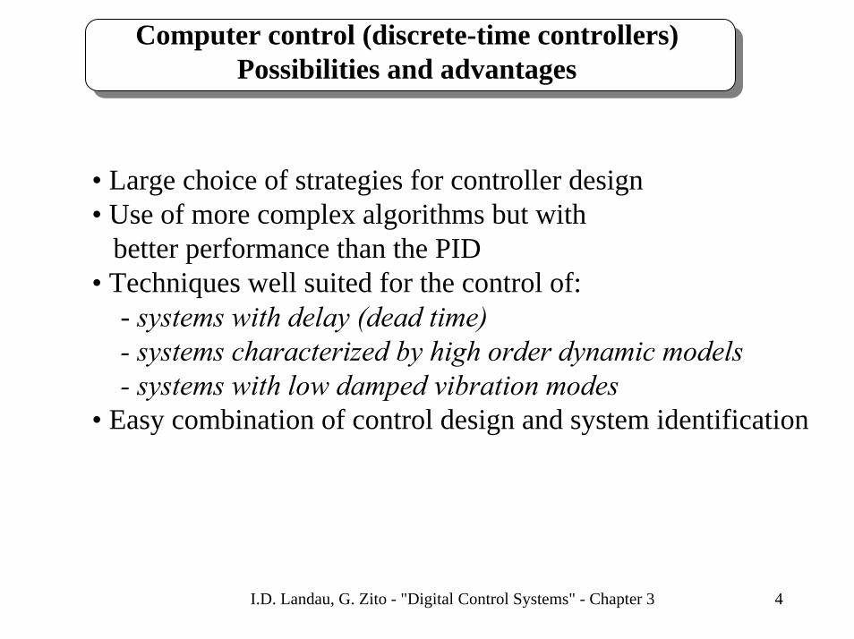
Computer control (discrete-time controllers)Possibilities and advantages
• Large choice of strategies for controller design• Use of more complex algorithms but with
better performance than the PID• Techniques well suited for the control of:
- systems with delay (dead time)- systems characterized by high order dynamic models- systems with low damped vibration modes
• Easy combination of control design and system identification
I.D. Landau, G. Zito - "Digital Control Systems" - Chapter 3 5
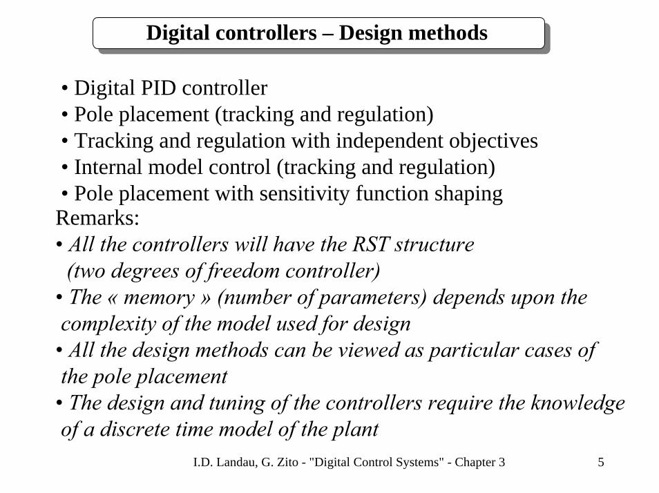
Digital controllers – Design methods
• Digital PID controller• Pole placement (tracking and regulation)• Tracking and regulation with independent objectives• Internal model control (tracking and regulation)• Pole placement with sensitivity function shaping
Remarks:• All the controllers will have the RST structure
(two degrees of freedom controller)• The « memory » (number of parameters) depends upon the complexity of the model used for design
• All the design methods can be viewed as particular cases of the pole placement
• The design and tuning of the controllers require the knowledge of a discrete time model of the plant
I.D. Landau, G. Zito - "Digital Control Systems" - Chapter 3 6
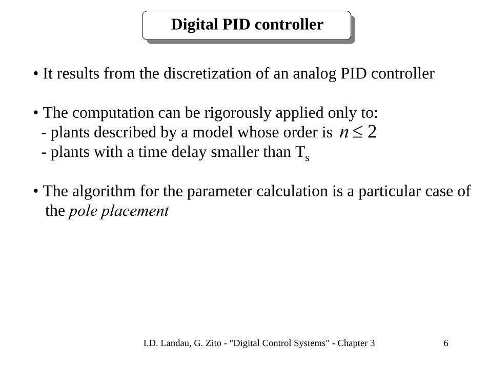
Digital PID controller
• It results from the discretization of an analog PID controller
• The computation can be rigorously applied only to:- plants described by a model whose order is- plants with a time delay smaller than Ts
• The algorithm for the parameter calculation is a particular case of the pole placement
2≤n
I.D. Landau, G. Zito - "Digital Control Systems" - Chapter 3 7
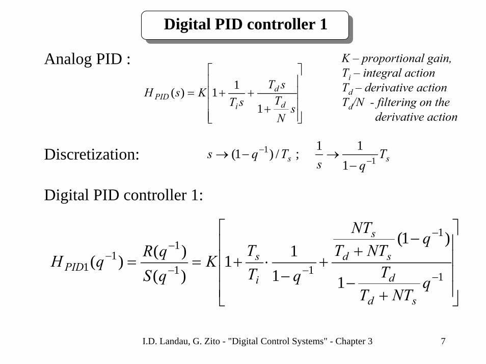
Digital PID controller 1
Analog PID : K – proportional gain,Ti – integral actionTd – derivative actionTd/N - filtering on the
derivative action ⎥⎥⎥⎥
⎦
⎤
⎢⎢⎢⎢
⎣
⎡
+++=
sNT
sTsT
KsHd
d
iPID
1
11)(
ss Tqs
Tqs 11
111;/)1(
−−
−→−→Discretization:
Digital PID controller 1:
⎥⎥⎥⎥
⎦
⎤
⎢⎢⎢⎢
⎣
⎡
+−
−+
+−
⋅+==−
−
−−
−−
1
1
11
11
11
)1(
111
)()()(
qNTT
T
qNTT
NT
qTT
KqSqRqH
sd
d
sd
s
i
sPID

I.D. Landau, G. Zito - "Digital Control Systems" - Chapter 3 8
Digital PID controller 1
)()()( 1
11
1 −
−− =
qSqRqHPID
22
110
1)( −−− ++= qrqrrqR 22
11
11
11 1)'1)(1()( −−−−− ++=+−= qsqsqsqqS
⎥⎥⎦
⎤
⎢⎢⎣
⎡−⎟⎟
⎠
⎞⎜⎜⎝
⎛++= 12111 N
TT
sKri
s )1(12 NKsr +−=⎟⎟⎠
⎞⎜⎜⎝
⎛−+= 10 1 Ns
TT
Kri
s
sd
d
NTTT
s+
−=′1
Remark:• The digital PID controller has 4 parameters (as the analog PID)• Common factor in the denominator: (integrator)• filtering action: factor in the denominator
)1( 1−− q)'1( 1
1−+ qs

I.D. Landau, G. Zito - "Digital Control Systems" - Chapter 3 9
Digital PID controller 1
y(t)
+
-
r(t) u(t)
R/S B/A
PLANT
r(t)
R
1/S B/A
PLANT
u(t) y(t)+
-
T=R
⇔
Structure RST with T = R
T.F. of the closed loop (r y)
)()()(
)()()()()()()( 1
11
1111
111
−
−−
−−−−
−−− =
+=
qPqRqB
qRqBqSqAqRqBqHCL
)( 1−qP defines the closed loop polesThe controller introduces supplementary zeros (R)
I.D. Landau, G. Zito - "Digital Control Systems" - Chapter 3 10
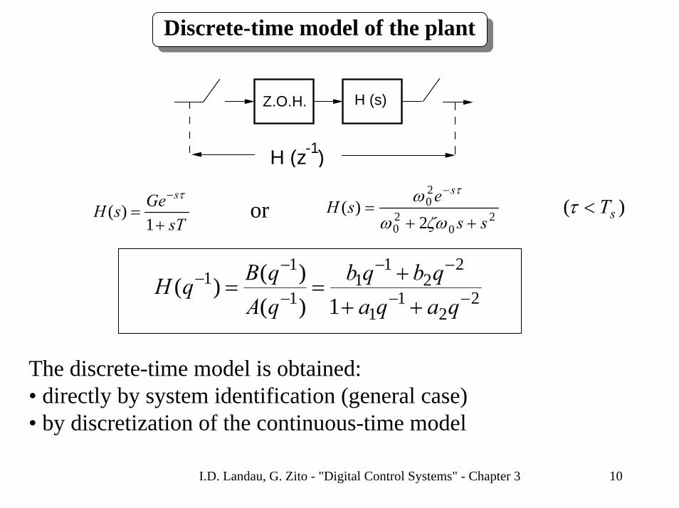
Discrete-time model of the plant
Z.O.H.
H (z )-1
H (s)
sTGesH
s
+=
−
1)(
τ
20
20
20
2)(
sse
sHs
++=
−
ζωωω τ
)( sTor <τ
22
11
22
11
1
11
1)()()( −−
−−
−
−−
+++
==qaqa
qbqbqAqBqH
The discrete-time model is obtained:• directly by system identification (general case)• by discretization of the continuous-time model

I.D. Landau, G. Zito - "Digital Control Systems" - Chapter 3 11
Parameter computation of the digital PID controller 1
Performances specifications :
)()(
)()()()()()()( 1
1
1111
111
−
−
−−−−
−−− =
+=
qPqB
qRqBqSqAqRqBqH M
CL (*)
)( 1−qBM cannot be imposed (as B is kept andThe controller introduces supplementary zeros)The characteristic polynomial (P) of the closed loop is specified :
22
11
1 ''1)( −−− ++== qpqpqP
Continuous-timespecification(tM, M)
2nd order (ω0, ζ)discretization
sT )( 1−qP5.125.0 0 ≤≤ sTω
17.0 ≤≤ ζ

I.D. Landau, G. Zito - "Digital Control Systems" - Chapter 3 12
Parameter computation of the digital PID controller 1
)(/)( 11 −− qAqB)( 1−qP
- Known (or identified) plant model :- Desired performances (CL poles):
)(;)( 11 −− qSqRTo be computed : From (*) – slide 11, one solves:
)()()()()( 11111 −−−−− += qRqBqSqAqP
? ?
)()()()(
))((
)1)(1)(1(
)()()()(1)(
1111
22
110
22
11
11
122
11
111122
11
1
−−−−
−−−−
−−−−
−−−−−−−
+′′=
++++
′+−++=
+=′+′+=
qRqBqSqA
qrqrrqbqb
qsqqaqa
qRqBqSqAqpqpqP
11
1 1)( −− ′+=′ qsqS)1()1)(()( 33
22
11
111 −−−−−− ′+′+′+=−=′ qaqaqaqqAqA
Tools : WinREG, bezoutd.sci(.m)
I.D. Landau, G. Zito - "Digital Control Systems" - Chapter 3 13
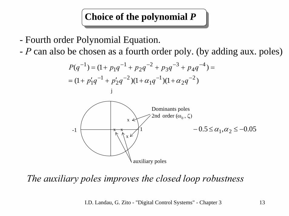
Choice of the polynomial P
- Fourth order Polynomial Equation.- P can also be chosen as a fourth order poly. (by adding aux. poles)
)1)(1)(1(
)1()(2
21
12
21
1
44
33
22
11
1
−−−−
−−−−−
++′+′+=
=++++=
qqqpqp
qpqpqpqpqP
ααj
05.0,5.0 21 −≤≤− ααx xx
x
1
Dominants poles2nd order (ω0 , ζ)
auxiliary poles
-1
The auxiliary poles improves the closed loop robustness

I.D. Landau, G. Zito - "Digital Control Systems" - Chapter 3 14
Equivalent analog PID controller parameters
21
21110
)1()2(
srsrsr
K′+
′+−−′=
210
1)1(rrr
sKTT si ++′+
⋅=
1
1
1 sTs
NT sd
′+′−
=3
1
21101
)1( sKrrsrs
TT sd ′+
+′−′⋅=
The continuous equivalent does not always exist!
0'1 1 ≤≤− sExistence condition: (Td/N > 0)
Digital PID controller always can be implemented even if :(no equivalent achievable performance with an analog PI)
1'0 1 ≤≤ s
I.D. Landau, G. Zito - "Digital Control Systems" - Chapter 3 15
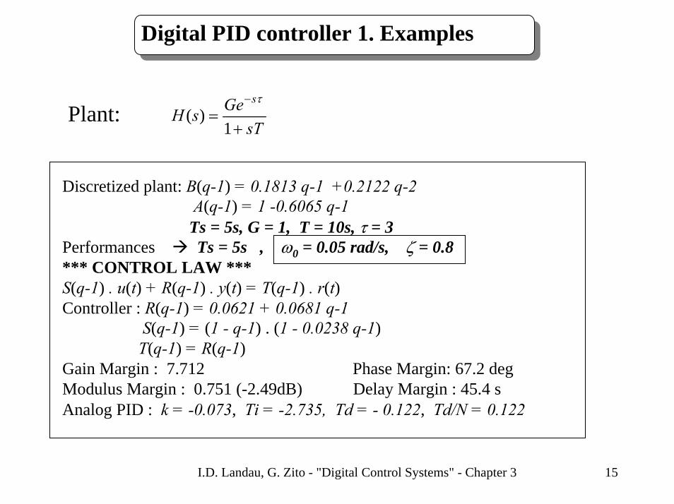
Digital PID controller 1. Examples
sTGesH
s
+=
−
1)(
τPlant:
Discretized plant: B(q-1) = 0.1813 q-1 +0.2122 q-2A(q-1) = 1 -0.6065 q-1
Ts = 5s, G = 1, T = 10s, τ = 3Performances Ts = 5s , ω0 = 0.05 rad/s, ζ = 0.8*** CONTROL LAW *** S(q-1) . u(t) + R(q-1) . y(t) = T(q-1) . r(t)Controller : R(q-1) = 0.0621 + 0.0681 q-1
S(q-1) = (1 - q-1) . (1 - 0.0238 q-1)T(q-1) = R(q-1)
Gain Margin : 7.712 Phase Margin: 67.2 degModulus Margin : 0.751 (-2.49dB) Delay Margin : 45.4 sAnalog PID : k = -0.073, Ti = -2.735, Td = - 0.122, Td/N = 0.122

I.D. Landau, G. Zito - "Digital Control Systems" - Chapter 3 16
Performances: ω0 = 0.05 rad/s, ζ = 0.8
0 10 20 30 40 50 60 70 80 90 1000
0.2
0.4
0.6
0.8
1
Plant Output
Time (t/Ts)
0 10 20 30 40 50 60 70 80 90 1000
0.5
1
1.5
Control Signal
Time (t/Ts)
Closed Loop response slower than Open Loop response.The specified ω0 should be increased
I.D. Landau, G. Zito - "Digital Control Systems" - Chapter 3 17
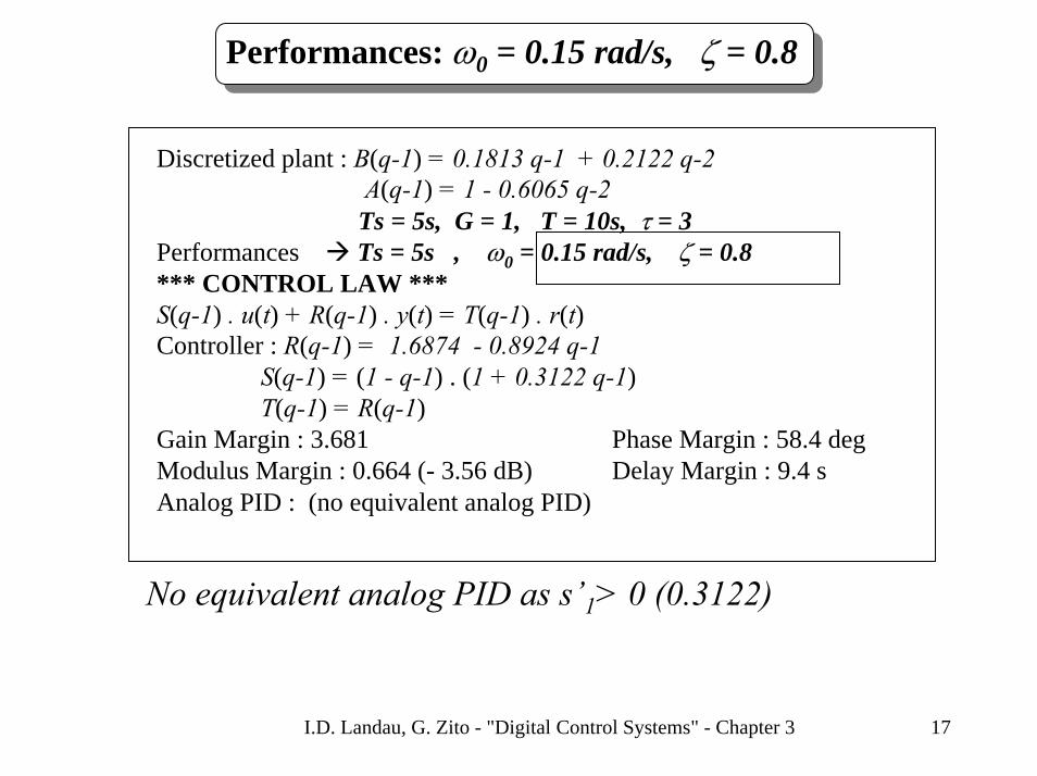
Performances: ω0 = 0.15 rad/s, ζ = 0.8
Discretized plant : B(q-1) = 0.1813 q-1 + 0.2122 q-2A(q-1) = 1 - 0.6065 q-2
Ts = 5s, G = 1, T = 10s, τ = 3Performances Ts = 5s , ω0 = 0.15 rad/s, ζ = 0.8*** CONTROL LAW *** S(q-1) . u(t) + R(q-1) . y(t) = T(q-1) . r(t)Controller : R(q-1) = 1.6874 - 0.8924 q-1
S(q-1) = (1 - q-1) . (1 + 0.3122 q-1)T(q-1) = R(q-1)
Gain Margin : 3.681 Phase Margin : 58.4 degModulus Margin : 0.664 (- 3.56 dB) Delay Margin : 9.4 sAnalog PID : (no equivalent analog PID)
No equivalent analog PID as s’1> 0 (0.3122)

I.D. Landau, G. Zito - "Digital Control Systems" - Chapter 3 18
Performances: ω0 = 0.15 rad/s, ζ = 0.8
0 10 20 30 40 50 60 70 80 90 1000
0.2
0.4
0.6
0.8
1
Plant Output
Time (t/Ts)
0 10 20 30 40 50 60 70 80 90 1000
0.5
1
1.5
Control Signal
Time (t/Ts)
- Faster response- An overshoot appears because of the zeros introduced by R
I.D. Landau, G. Zito - "Digital Control Systems" - Chapter 3 19
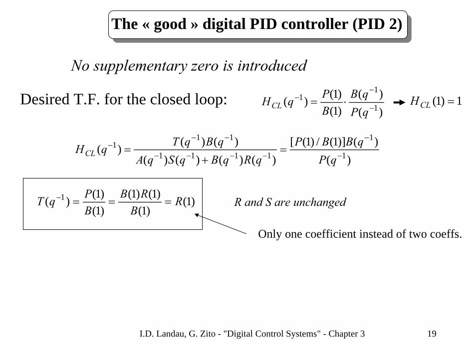
The « good » digital PID controller (PID 2)
No supplementary zero is introduced
)()(
)1()1()( 1
11
−
−− ⋅=
qPqB
BPqHCLDesired T.F. for the closed loop: 1)1( =CLH
)()()]1(/)1([
)()()()()()()( 1
1
1111
111
−
−
−−−−
−−− =
+=
qPqBBP
qRqBqSqAqBqTqHCL
)1()1(
)1()1()1()1()( 1 R
BRB
BPqT ===− R and S are unchanged
Only one coefficient instead of two coeffs.

I.D. Landau, G. Zito - "Digital Control Systems" - Chapter 3 20
Continuous time PID corresponding to digital PID 2
k d s
1 + - - - -T N
s
+
+ -
- PLANT
Kd
-
KT d s
K____Ti s
r(t) u(t) y(t)
1/ ( )
------------------1
1 + -----T
N s
d
The proportional and derivative actions only act on the measure
1
1
1 sTs
NT sd
′+′−
=)1)(2(
)1(
121
2111
srrrsrsTT sd ′++
−′+′⋅=
210
21 )2(rrr
rrTT si +++−
⋅=1
21
1)2(
srrK
′++−
=
I.D. Landau, G. Zito - "Digital Control Systems" - Chapter 3 21
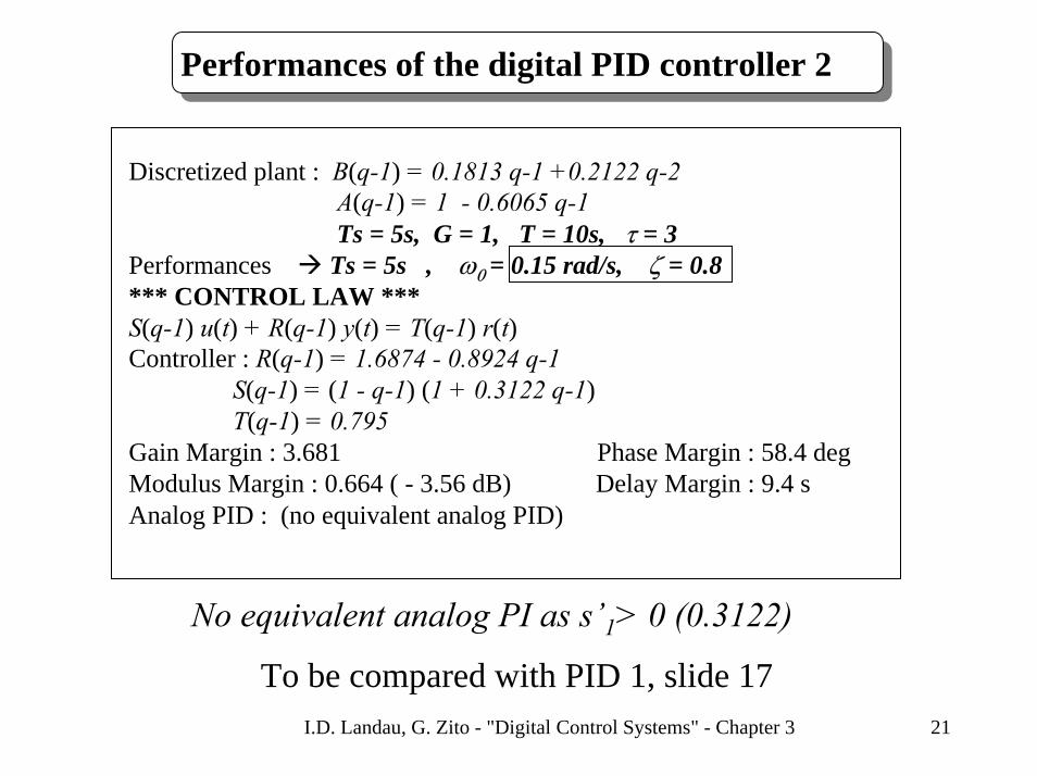
Performances of the digital PID controller 2
Discretized plant : B(q-1) = 0.1813 q-1 +0.2122 q-2A(q-1) = 1 - 0.6065 q-1Ts = 5s, G = 1, T = 10s, τ = 3
Performances Ts = 5s , ω0 = 0.15 rad/s, ζ = 0.8*** CONTROL LAW *** S(q-1) u(t) + R(q-1) y(t) = T(q-1) r(t)Controller : R(q-1) = 1.6874 - 0.8924 q-1
S(q-1) = (1 - q-1) (1 + 0.3122 q-1)T(q-1) = 0.795
Gain Margin : 3.681 Phase Margin : 58.4 degModulus Margin : 0.664 ( - 3.56 dB) Delay Margin : 9.4 sAnalog PID : (no equivalent analog PID)
No equivalent analog PI as s’1> 0 (0.3122)
To be compared with PID 1, slide 17

I.D. Landau, G. Zito - "Digital Control Systems" - Chapter 3 22
Performances of the digital PID controller 2
ω0 = 0.15 rad/s, ζ = 0.8
Reduced overshoot (corresponding to ζ = 0.8). Same response for disturbance rejection
To be compared with slide 18
0 10 20 30 40 50 60 70 80 90 1000
0.2
0.4
0.6
0.8
1
Plant Output
Time (t/Ts)
0 10 20 30 40 50 60 70 80 90 1000
0.5
1
1.5
Control Signal
Time (t/Ts)
I.D. Landau, G. Zito - "Digital Control Systems" - Chapter 3 23
Auxiliary poles effects
The auxiliary poles reduce the input sensitivity function Sup at highfrequencies without degrading the closed loop performances
Better robustness and reduction of actuator stress

I.D. Landau, G. Zito - "Digital Control Systems" - Chapter 3 24
Digital PID controller : conclusions
• RST Canonical structure
• Equivalent analog PID if
• Used with 1st or 2nd order systems with delay < Ts
• For a delay the analog PID leads to closed loop responsesslower than open loop responses
• The digital PID controller gives better performances for systemswith delay (but there is no equivalent in continuous-time)
• The digital PID controller 2 leads to a step response with a smallerovershoot than PID 1
0'1 1 ≤≤− s
T25.0≥τ
I.D. Landau, G. Zito - "Digital Control Systems" - Chapter 3 25
Pole placement
The pole placement allows to design a R-S-T controller for• stable or unstable systems• without restriction upon the degrees of A and B polynomials• without restrictions upon the plant model zeros (stable or unstable)
It is a method that does not simplify the plant model zeros
The digital PID can be designed using pole placement

I.D. Landau, G. Zito - "Digital Control Systems" - Chapter 3 26
Structure
) ------------1
(q- 1
)---------q
- dB
A
PLANT
R(q- 1
)
--------------------q
- dB(q
- 1)
(q- 1
)
S
P
r(t) y(t)+
-
T( ) q - 1
p(t)
++
)()()( 1
11
−
−−− =
qAqBqqH
dPlant:
)(...)( 1*122
11
1 −−−−−− =+++= qBqqbqbqbqB BB
nn
AA
nn qaqaqA −−− +++= ...1)( 1
11

I.D. Landau, G. Zito - "Digital Control Systems" - Chapter 3 27
Pole placement
Closed loop T.F. (r y) (reference tracking)
)()()(
)()()()()()()( 1
11
1111
111
−
−−−
−−−−−
−−−− =
+=
qPqBqTq
qRqBqqSqAqBqTqqH
d
d
d
BF
....1)()()()()( 22
11
11111 +++=+= −−−−−−−− qpqpqRqBqqSqAqP d
Defines the (desired )closed loop poles
Closed loop T.F. (p y) (disturbance rejection)
)()()(
)()()()()()()(
1
11
1111
111
−
−−
−−−−−
−−− =
+=
qPqSqA
qRqBqqSqAqSqAqS
dyp
Output sensitivity function

I.D. Landau, G. Zito - "Digital Control Systems" - Chapter 3 28
Choice of desired closed loop poles (polynomial P)
)()()( 111 −−− = qPqPqP FD
Dominant poles Auxiliary poles
Choice of PD(q-1)(dominant poles)Specificationin continuous time(tM, M)
2nd order (ω0, ζ)discretization
eT )( 1−qPD
5.125.0 0 ≤≤ eTω17.0 ≤≤ ζ
Auxiliary poles
• Auxiliary poles are introduced for robustness purposes• They usually are selected to be faster than the dominant poles

I.D. Landau, G. Zito - "Digital Control Systems" - Chapter 3 29
Regulation( computation of R(q-1) and S(q-1))
)()()()()( 11111 −−−−−− =+ qPqRqBqqSqA d
? ?
)(deg 1−= qAnA )(deg 1−= qBnBA and B do not have
common factors
(*)(Bezout)
unique minimal solution for :1)(deg 1 −++≤= − dnnqPn BAP
1)(deg 1 −+== − dnqSn BS 1)(deg 1 −== −AR nqRn
)(*1...1)( 1111
1 −−−−− +=++= qSqqsqsqS S
S
nn
R
R
nn qrqrrqR −−− ++= ...)( 1
101
I.D. Landau, G. Zito - "Digital Control Systems" - Chapter 3 30
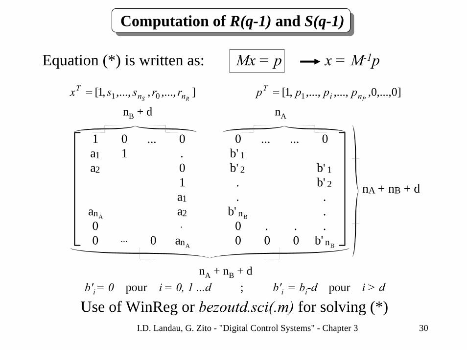
Computation of R(q-1) and S(q-1)
Equation (*) is written as: Mx = p x = M-1p
],...,,,...,,1[ 01 RS nnT rrssx = ]0,...,0,,...,,...,,1[ 1 Pni
T pppp =
1 0 ... 0a1 1 .a2 0
1a1
anA a20 .
0 ... 0 anA
0 ... ... 0b' 1b' 2 b' 1. b' 2. .
b' nB .0 . . .0 0 0 b' nB
nA + nB + d
nB + d nA
nA + nB + db'i = 0 pour i = 0, 1 ...d ; b'i = bi-d pour i > d
Use of WinReg or bezoutd.sci(.m) for solving (*)

I.D. Landau, G. Zito - "Digital Control Systems" - Chapter 3 31
Structure of R(q-1) and S(q-1)
R and S include pre-specified fixed parts (ex: integrator))()(')( 111 −−− = qHqSqS S)()(')( 111 −−− = qHqRqR R
HR, HS, - pre-specified polynomials
'
''...'')(' 1
101 R
R
nn qrqrrqR −−− ++= '
''...'1)(' 1
11 S
S
nn qsqsqS −−− ++=
•The pre specified filters HR and HS will allow to impose certain properties of the closed loop.•They can influence performance and/or robustness

I.D. Landau, G. Zito - "Digital Control Systems" - Chapter 3 32
Fixed parts (HR , HS). Examples
Zero steady state error (Syp should be null at certain frequencies)
)()()()(
)( 1
1111
−
−−−− ′
=qP
qSqHqAqS S
yp
Step disturbance : Sinusoidal disturbance : sS TqqH ωαα cos2;1 21 −=++= −−
11 1)( −− −= qqHS
Signal blocking (Sup should be null at certain frequencies)
)()()()(
)( 1
1111
−
−−−− ′
−=qP
qRqHqAqS R
up
sR TqqH ωββ cos2;1 21 −=++= −−
2,1;)1( 1 =+=Sinusoidal signal:Blocking at 0.5fS:
− nqH nR

I.D. Landau, G. Zito - "Digital Control Systems" - Chapter 3 33
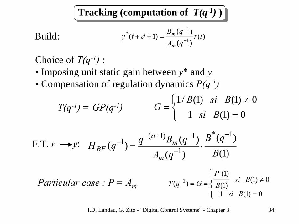
Tracking (computation of T(q-1) )
------------q
- 1Bm
Am
Ideal case
r (t) y* (t)
desiredtrajectory for y (t)
t
y
r
*
Tracking referencemodel (Hm)
)()(
)( 1
111
−
−−− =
qAqBq
qHm
mm
...)( 110
1 ++= −− qbbqB mmm
...1)( 22
11
1 +++= −−− qaqaqA mmm
Specificationin continuous time(tM, M)
2nd order (ω0, ζ)discretization
sT )( 1−qHm
5.125.0 0 ≤≤ sTω17.0 ≤≤ ζ
The ideal case can not be obtained (delay, plant zeros)Objective : to approach y*(t)
)()(
)()( 1
1)1(* tr
qAqBq
tym
md
−
−+−
=
I.D. Landau, G. Zito - "Digital Control Systems" - Chapter 3 34
Tracking (computation of T(q-1) )
)()()(
)1( 1
1* tr
qAqB
dtym
m−
−
=++Build:
Choice of T(q-1) :• Imposing unit static gain between y* and y• Compensation of regulation dynamics P(q-1)
⎩⎨⎧
=≠
=0)1(1
0)1()1(/1Bsi
BsiBGT(q-1) = GP(q-1)
F.T. r y:)1(
)(
)()()(
1*
1
1)1(1
BqB
qAqBqqH
m
md
BF
−
−
−+−− ⋅=
⎪⎩
⎪⎨⎧
=
≠==−
0)1(1
0)1()1()1(
)( 1
Bsi
BsiBP
GqTParticular case : P = Am

I.D. Landau, G. Zito - "Digital Control Systems" - Chapter 3 35
Pole placement. Tracking and regulation
+
-
R
1 q-d
BAS
TA
Bm
m
r(t)
y (t+d+1)*u(t) y(t)
q
-(d+1)
P(q -1 )q
-(d+1)
B*(q )-1
B*(q )
-1
B(1)q
-(d+1) B m(q )
B*(q )
-1-1
A m(q ) B(1)-1
)1(*)()()()()( 111 ++=+ −−− dtyqTtyqRtuqS

I.D. Landau, G. Zito - "Digital Control Systems" - Chapter 3 36
Pole placement. Control law
)()()()1()()( 1
1*1
−
−− −++=
qStyqRdtyqTtu
)1()()1()()()()()( *1*111 ++=++=+ −−−− dtyqTdtyqGPtyqRtuqS
)(1)( 1*11 −−− += qSqqS
)()()1()()1()()( 11**1 tyqRtuqSdtGyqPtu −−− −−−++=
)()()(
)1( 1
1* tr
qAqB
dtym
m−
−
=++
)(1)( 1*11 −−− += qAqqA mm
)()()()()1( 11** trqBdtyqAdty mm−− ++−=++
...)( 110
1 ++= −− qbbqB mmm ...1)( 22
11
1 +++= −−− qaqaqA mmm

I.D. Landau, G. Zito - "Digital Control Systems" - Chapter 3 37
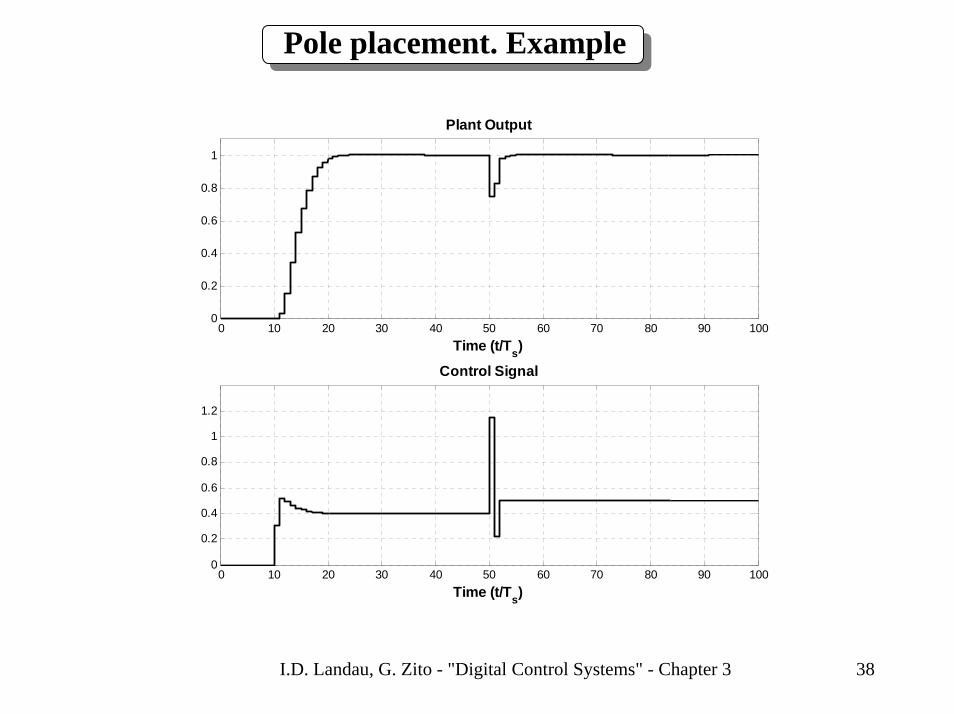
Pole placement. Example
Plant : d=0B(q-1) = 0.1 q-1 + 0.2 q-2A(q-1) = 1 - 1.3 q-1 + 0.42 q-2
Bm(q-1) = 0.0927 + 0.0687 q-1Tracking dynamics
Am (q-1) = 1 - 1.2451q-1 + 0.4066 q-2Ts = 1s , ω0 = 0.5 rad/s, ζ = 0.9
Regulation dynamics P (q-1) = 1 - 1.3741 q-1 + 0.4867 q-2Ts = 1s , ω0 = 0.4 rad/s, ζ = 0.9
Pre-specifications : Integrator*** CONTROL LAW ***S (q-1) u(t) + R (q-1) y(t) = T (q-1) y*(t+d+1)y*(t+d+1) = [Bm(q-1)/Am(q-1)] r(t)Controller : R(q-1) = 3 - 3.94 q-1 + 1.3141 q-2
S(q-1) = 1 - 0.3742 q-1 - 0.6258 q-2T(q-1) = 3.333 - 4.5806 q-1 + 1.6225 q-2
Gain margin : 2.703 Phase margin : 65.4 degModulus margin : 0.618 (- 4.19 dB) Delay margin: 2.1. s
I.D. Landau, G. Zito - "Digital Control Systems" - Chapter 3 38
Pole placement. Example
0 10 20 30 40 50 60 70 80 90 1000
0.2
0.4
0.6
0.8
1
Plant Output
Time (t/Ts)
0 10 20 30 40 50 60 70 80 90 1000
0.2
0.4
0.6
0.8
1
1.2
Control Signal
Time (t/Ts)
I.D. Landau, G. Zito - "Digital Control Systems" - Chapter 3 39
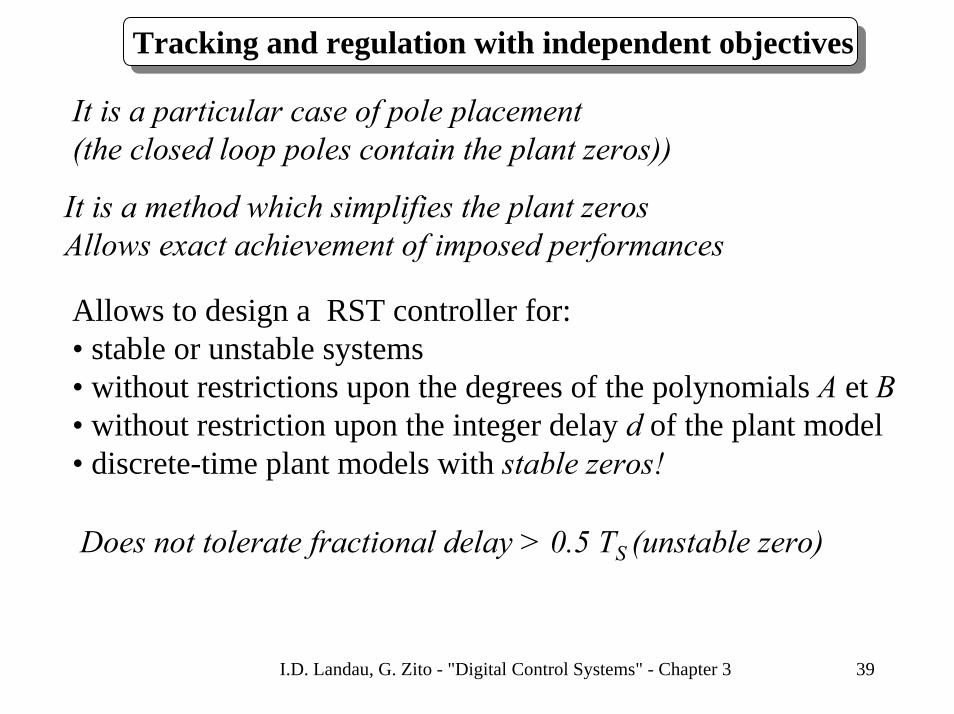
Tracking and regulation with independent objectives
It is a particular case of pole placement(the closed loop poles contain the plant zeros))
It is a method which simplifies the plant zerosAllows exact achievement of imposed performances
Allows to design a RST controller for:• stable or unstable systems• without restrictions upon the degrees of the polynomials A et B• without restriction upon the integer delay d of the plant model• discrete-time plant models with stable zeros!
Does not tolerate fractional delay > 0.5 TS (unstable zero)

I.D. Landau, G. Zito - "Digital Control Systems" - Chapter 3 40
Tracking and regulation with independent objectives
The model zeros should be stable and enough damped
-1 -0.5 0 0.5 1-1
-0.8
-0.6
-0.4
-0.2
0
0.2
0.4
0.6
0.8
1Zero Admissible Zone
Real Axis
Imag
Axi
sf0/fs = 0.4
0.4
0.3
0.3
0.2
0.2
0.1
0.1
ζ = 0.1 ζ = 0.2
Admissibility domain for the zeros of the discrete time model
I.D. Landau, G. Zito - "Digital Control Systems" - Chapter 3 41
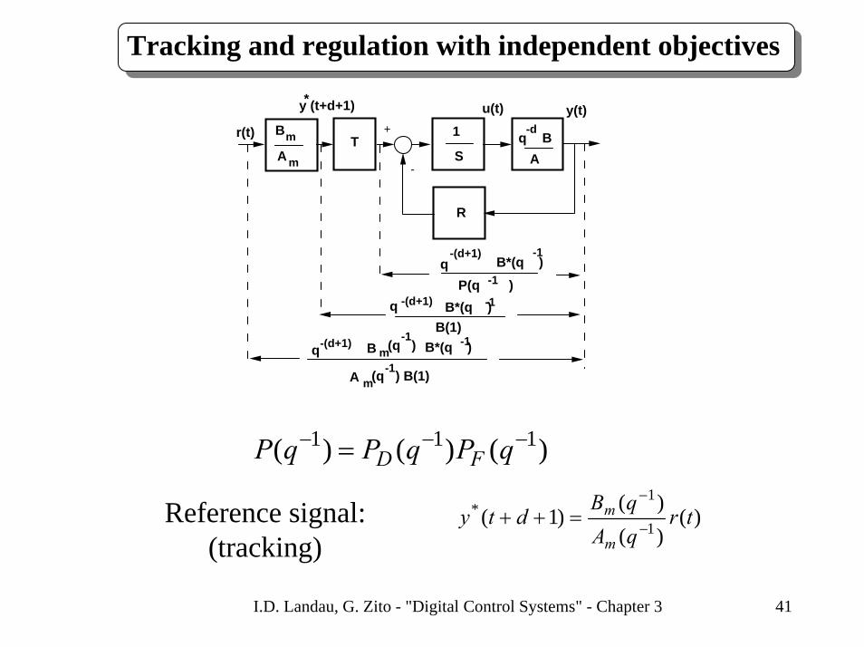
Tracking and regulation with independent objectives
+
-
R
1 q-d
BAS
TA
Bm
m
r(t)
y (t+d+1)*u(t) y(t)
q
-(d+1)
P(q -1 )q
-(d+1)
B*(q )-1
B*(q )
-1
B(1)q
-(d+1) B m(q )
B*(q )
-1-1
A m(q ) B(1)-1
)()()( 111 −−− = qPqPqP FD
)()()(
)1( 1
1* tr
qAqB
dtym
m−
−
=++Reference signal:(tracking)
I.D. Landau, G. Zito - "Digital Control Systems" - Chapter 3 42
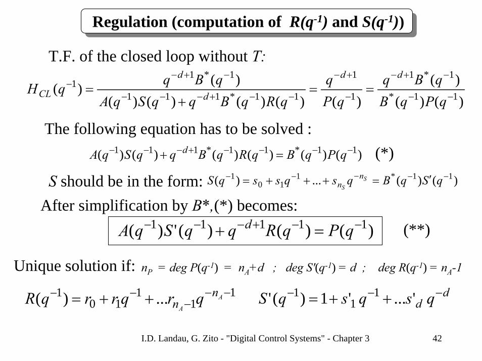
Regulation (computation of R(q-1) and S(q-1))
T.F. of the closed loop without T:
)()()(
)()()()()()()( 11*
1*1
1
1
11*111
1*11
−−
−+−
−
+−
−−+−−−
−+−− ==
+=
qPqBqBq
qPq
qRqBqqSqAqBqqH
dd
d
d
CL
The following equation has to be solved :(*))()()()()()( 11*11*111 −−−−+−−− =+ qPqBqRqBqqSqA d
S should be in the form: )()(...)( 11*110
1 −−−−− ′=+++= qSqBqsqssqS SS
nn
After simplification by B*,(*) becomes:)()()(')( 11111 −−+−−− =+ qPqRqqSqA d (**)
Unique solution if: nP = deg P(q-1) = nA+d ; deg S'(q-1) = d ; deg R(q-1) = nA-1
11
110
1 ...)( −−−
−− ++= A
A
nn qrqrrqR d
d qsqsqS −−− ++= '...'1)(' 11
1
I.D. Landau, G. Zito - "Digital Control Systems" - Chapter 3 43
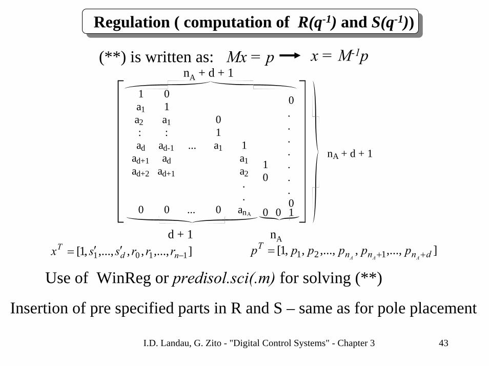
Regulation ( computation of R(q-1) and S(q-1))
(**) is written as: Mx = p
1 0 a1 1 a2 a1 0: : 1ad ad-1 ... a1 1
ad+1 ad a1ad+2 ad+1 a2
. .0 0 ... 0 anA
0 . .
. .
1 . 0 .
. 00 0 1
nA + d + 1
nA + d + 1
d + 1 nA],...,,,,...,,1[ 1101 −′′= nd
T rrrssx ],...,,,...,,,1[ 121 dnnnT
AAApppppp ++=
Use of WinReg or predisol.sci(.m) for solving (**)
x = M-1p
Insertion of pre specified parts in R and S – same as for pole placement
I.D. Landau, G. Zito - "Digital Control Systems" - Chapter 3 44
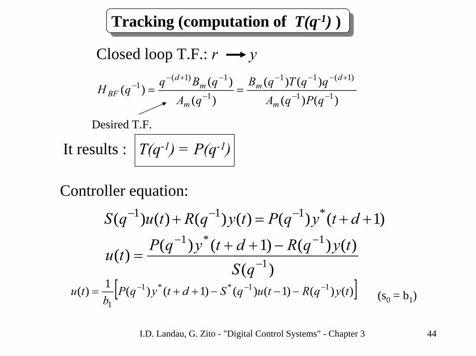
Tracking (computation of T(q-1) )
Closed loop T.F.: r y
)()()()(
)()(
)( 11
)1(11
1
1)1(1
−−
+−−−
−
−+−− ==
qPqAqqTqB
qAqBq
qHm
dm
m
md
BF
Desired T.F.
It results : T(q-1) = P(q-1)
Controller equation:
)1()()()()()( *111 ++=+ −−− dtyqPtyqRtuqS
)()()()1()()( 1
1*1
−
−− −++=
qStyqRdtyqPtu
[ ])()()1()()1()(1)( 11**1
1tyqRtuqSdtyqP
btu −−− −−−++= (s0 = b1)

I.D. Landau, G. Zito - "Digital Control Systems" - Chapter 3 45
Tracking and regulation with independent objectives. Examples
Plant : d = 0B(q-1) = 0.2 q-1 + 0.1 q-2A(q-1) = 1 - 1.3 q-1 + 0.42 q-2
Bm (q-1) = 0.0927 + 0.0687 q-1Tracking dynamics
Am (q-1) = 1 - 1.2451q-1 + 0.4066 q-2Ts = 1s , ω0 = 0.5 rad/s, ζ = 0.9
Regulation dynamics P (q-1) = 1 - 1.3741 q-1 + 0.4867 q-2Ts = 1s , ω0 = 0.4 rad/s, ζ = 0.9
Pre-specifications : Integrator*** CONTROL LAW ***S (q-1) u(t) + R (q-1) y(t) = T (q-1) y*(t+d+1)y*(t+d+1) = [Bm (q-1)/Am (q-1)] . r(t)Controller : R(q-1) = 0.9258 - 1.2332 q-1 + 0.42 q-2
S(q-1) = 0.2 - 0.1 q-1 - 0.1 q-2T(q-1) = P(q-1)
Gain margin : 2.109 Phase margin : 65.3 degModulus margin : 0.526 (- 5.58 dB) Delay margin : 1.2
I.D. Landau, G. Zito - "Digital Control Systems" - Chapter 3 46
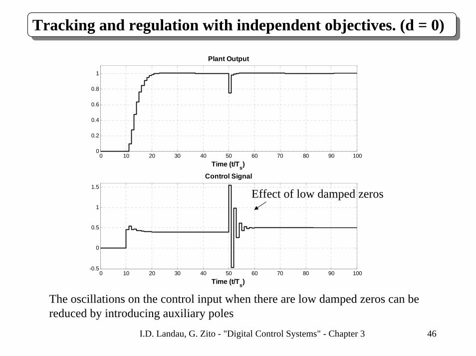
Tracking and regulation with independent objectives. (d = 0)
0 10 20 30 40 50 60 70 80 90 1000
0.2
0.4
0.6
0.8
1
Plant Output
Time (t/Ts)
0 10 20 30 40 50 60 70 80 90 100-0.5
0
0.5
1
1.5
Control Signal
Time (t/Ts)
Effect of low damped zeros
The oscillations on the control input when there are low damped zeros can bereduced by introducing auxiliary poles

I.D. Landau, G. Zito - "Digital Control Systems" - Chapter 3 47
Internal model control -Tracking and regulation
It is a particular case of the pole placementThe dominant poles are those of the plant modelDoes not allow to accelerate the closed loop response
Allows to design a RST controller for:• well damped stable systems• without restrictions upon the degrees of the polynomial A and B• without restrictions upon the delay of the discrete time model
The plant model should be stable and well damped !
Often used for the systems featuring a large delay
Remark: The name is misleading since it has nothing in common with the“internal model principle”
I.D. Landau, G. Zito - "Digital Control Systems" - Chapter 3 48
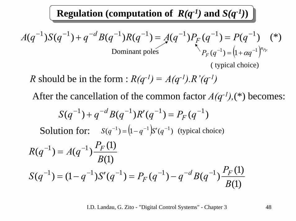
Regulation (computation of R(q-1) and S(q-1))
)()()()()()()( 1111111 −−−−−−−− ==+ qPqPqAqRqBqqSqA Fd
Dominant poles ( ) FPnF qqP 11 1)( −− += α
(*)
( typical choice)
R should be in the form : R(q-1) = A(q-1).R’(q-1)
After the cancellation of the common factor A(q-1),(*) becomes:
)()()()( 1111 −−−−− =′+ qPqRqBqqS Fd
( ) )(1)( 111 −−− ′−= qSqqS (typical choice) Solution for:
)1()1()()( 11
BPqAqR F−− =
)1()1(
)()()()1()( 11111
BP
qBqqPqSqqS FdF
−−−−−− −=′−=

I.D. Landau, G. Zito - "Digital Control Systems" - Chapter 3 49
Tracking (computation of T(q-1) )
)1(/)()()( 111 BqPqAqT F−−− =
Particular case : Am = APF (tracking dynamics = regulation dynamics)
)1()1()1()1()( 1
BPATqT F==− (cancellation of the tracking reference model)

Interpretation of the internal model control
Equivalent scheme
I.D. Landau, G. Zito - "Digital Control Systems" - Chapter 3 50
( )
)()()1(
1)()1(
1)(
)()(
1)()()1()1()(
1111
0
11
0
111
0
−−−−
−−
−−−
==
=
==
qPqAB
qPB
qT
qPqS
qHforqABPqR
F
F
RF
T0
+
-
-1/S0 Plant
ABdq−
Model
y*(t+d+1) u(t)
(t)y
y(t)
R0
The plant model(prediction model)is an element of thecontrol scheme
+
Feedback on thePrediction error
Rem.: For all the strategies one can show the presence of the plant model in the controller
I.D. Landau, G. Zito - "Digital Control Systems" - Chapter 3 51
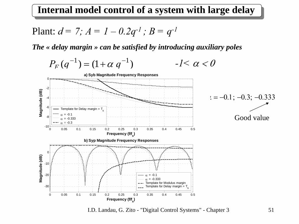
Internal model control of a system with large delay
Plant: d = 7; A = 1 – 0.2q-1 ; B = q-1
The « delay margin » can be satisfied by introducing auxiliary poles
) 1()( 11 −− += qqPF α -1< α < 0
α = −0.1; −0.3; −0.333
Good value
0 0.05 0.1 0.15 0.2 0.25 0.3 0.35 0.4 0.45 0.5
-30
-20
-10
0
b) Syp Magnitude Frequency Responses
Frequency (f/fs)
Mag
nitu
de (d
B)
0 0.05 0.1 0.15 0.2 0.25 0.3 0.35 0.4 0.45 0.5-10
-8
-6
-4
-2
0a) Syb Magnitude Frequency Responses
Frequency (f/fs)
Mag
nitu
de (d
B)
α = -0.1α = -0.333Template for Modulus marginTemplate for Delay margin = Ts
Template for Delay margin = Tsα = -0.1α = -0.333α = -0.3

I.D. Landau, G. Zito - "Digital Control Systems" - Chapter 3 52
11 1)( −− += qqH R corresponds to the opening of the loop at 0.5fS
Internal model control of a system with large delay
See also:I.D. Landau (1995) : Robust digital control of systems with time delay (the Smith predictor revisited)Int. J. of Control, v.62,no.2 pp 325-347
0 0.05 0.1 0.15 0.2 0.25 0.3 0.35 0.4 0.45 0.5-30
-20
-10
0
b) Syp Magnitude Frequency Responses
Frequency (f/fs)
Mag
nitu
de (d
B)
0 0.05 0.1 0.15 0.2 0.25 0.3 0.35 0.4 0.45 0.5-10
-8
-6
-4
-2
0a) Syb Magnitude Frequency Responses
Frequency (f/fs)
Mag
nitu
de (d
B)
HR = 1, PF = 1 - 0.333q-1
HR = 1 + q-1, PF = 1
Template for Modulus marginTemplate for Delay margin = Ts
Template for Delay margin = TsHR = 1, PF = 1 - 0.333q-1
HR = 1 + q-1, PF = 1
I.D. Landau, G. Zito - "Digital Control Systems" - Chapter 3 53
Pole placement with sensitivity functions shaping
Performance specification for pole placement :• Desired dominant poles for the closed loop• The reference trajectory (tracking reference model)
Questions:• How to take into account the specifications in certain frequencyregions?
• How to guarantee the robustness of the controllers ?• How to take advantage from the degree of freedom forthe maximum number of poles which can be assigned ?
Answer:Shaping the sensitivity functions by:
- introducing auxiliary poles- introducing filters in the controllers
I.D. Landau, G. Zito - "Digital Control Systems" - Chapter 3 54
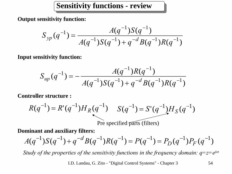
Sensitivity functions - reviewOutput sensitivity function:
)()()()()()()( 1111
111
−−−−−
−−−
+=
qRqBqqSqAqSqAqS dyp
Input sensitivity function:
)()()()()()()( 1111
111
−−−−−
−−−
+−=
qRqBqqSqAqRqAqS dup
Controller structure :
)()(')( 111 −−− = qHqRqR R )()(')( 111 −−− = qHqSqS S
)()()()()()()( 1111111 −−−−−−−− ==+ qPqPqPqRqBqqSqA FDd
Pre specified parts (filters)Dominant and auxiliary filters:
Study of the properties of the sensitivity functions in the frequency domain: q=z=ejω
I.D. Landau, G. Zito - "Digital Control Systems" - Chapter 3 55
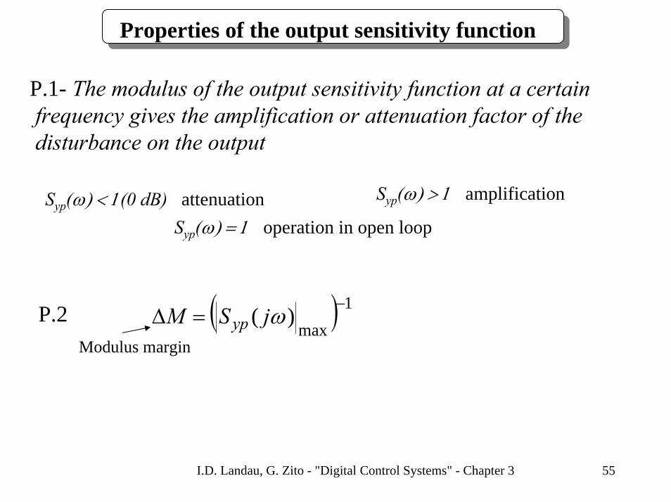
Properties of the output sensitivity function
P.1- The modulus of the output sensitivity function at a certainfrequency gives the amplification or attenuation factor of thedisturbance on the output
Syp(ω) > 1 amplificationSyp(ω) < 1(0 dB) attenuationSyp(ω) = 1 operation in open loop
( ) 1max
)(−
=∆ ωjSM ypModulus margin
P.2
I.D. Landau, G. Zito - "Digital Control Systems" - Chapter 3 56
Properties of the output sensitivity function
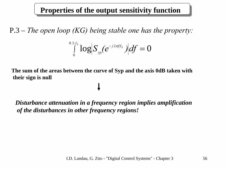
P.3 – The open loop (KG) being stable one has the property:
∫ =−SS
f.πf/fj
yp df)(eS50
0
2 0log
The sum of the areas between the curve of Syp and the axis 0dB taken withtheir sign is null
Disturbance attenuation in a frequency region implies amplificationof the disturbances in other frequency regions!
I.D. Landau, G. Zito - "Digital Control Systems" - Chapter 3 57
Properties of the output sensitivity function
0 0.05 0.1 0.15 0.2 0.25 0.3 0.35 0.4 0.45 0.5-25
-20
-15
-10
-5
0
5
Syp Magnitude Frequency Responses
Frequency (f/fs)
Mag
nitu
de (d
B)
ω = 0.4 rad/secω = 0.6 rad/secω = 1 rad/secTemplate for Modulus marginTemplate for Delay margin = Ts
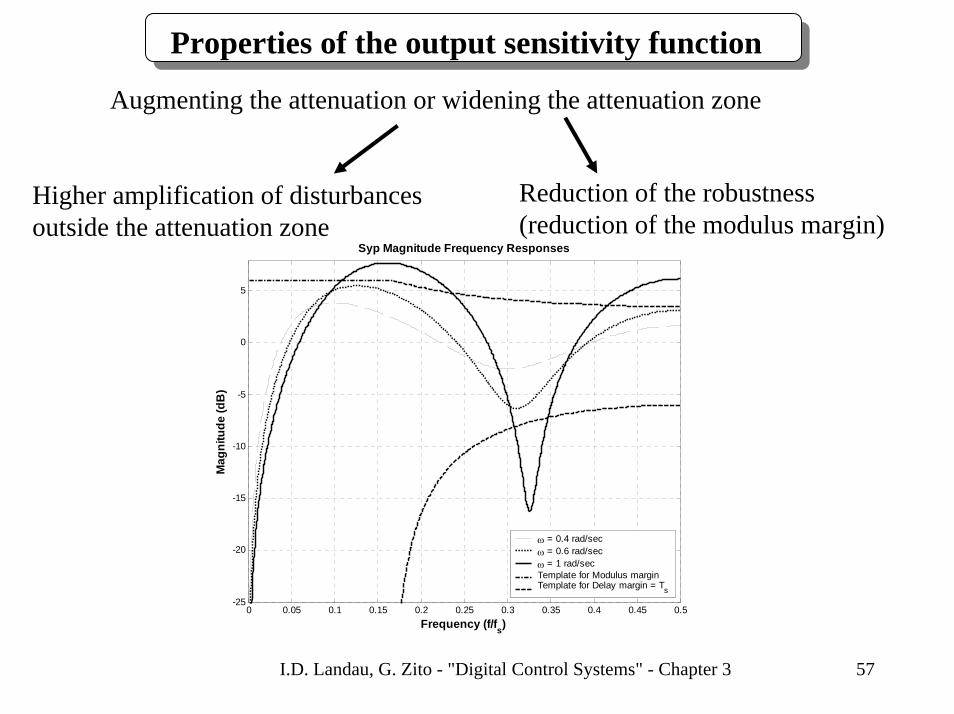
Augmenting the attenuation or widening the attenuation zone
Higher amplification of disturbancesoutside the attenuation zone
Reduction of the robustness(reduction of the modulus margin)
I.D. Landau, G. Zito - "Digital Control Systems" - Chapter 3 58
Properties of the output sensitivity function
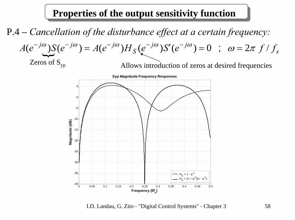
P.4 – Cancellation of the disturbance effect at a certain frequency:
sjj
Sjjj ffeSeHeAeSeA /20)()()()()( ; πωωωωωω ==′= −−−−−
{Zeros of Syp Allows introduction of zeros at desired frequencies
0 0.05 0.1 0.15 0.2 0.25 0.3 0.35 0.4 0.45 0.5-40
-35
-30
-25
-20
-15
-10
-5
0
5
Syp Magnitude Frequency Responses
Frequency (f/fs)
Mag
nitu
de (d
B)
HS = 1 - q-1
HS = (1 + q-2)(1 - q-1)

I.D. Landau, G. Zito - "Digital Control Systems" - Chapter 3 59
Properties of the output sensitivity function
P.5 - at frequencies where:)0(1)( dBjS yp =ω
sjj
Rjjj ffeReHeBeReB /20)()()()()( ** ; πωωωωωω ==′= −−−−−
0 0.05 0.1 0.15 0.2 0.25 0.3 0.35 0.4 0.45 0.5-25
-20
-15
-10
-5
0
5
Syp Magnitude Frequency Responses
Frequency (f/fs)
Mag
nitu
de (d
B)
HR = 1HR = 1 + q-2
Allows introduction of zeros at desired frequencies

I.D. Landau, G. Zito - "Digital Control Systems" - Chapter 3 60
0 0.05 0.1 0.15 0.2 0.25 0.3 0.35 0.4 0.45 0.5-25
-20
-15
-10
-5
0
5
Syp Magnitude Frequency Responses
Frequency (f/fs)
Mag
nitu
de (d
B)
PF = 1PF = (1 - 0.375q-1)2
Template for Modulus marginTemplate for Delay margin = Ts
P.6 – Asymptotically stable auxiliary poles (PF) lead (in general) to the reduction of in the attenuationband of 1/PF
)( ωjS yp
FPnF qpqP )1()( 11 −− ′+= 05.05.0 −≤′≤− p
DF PPP nnn −≤
In many applications, introduction of high frequency auxiliary polesis enough for assuring the required robustness margins
Properties of the output sensitivity function

I.D. Landau, G. Zito - "Digital Control Systems" - Chapter 3 61
Properties of the output sensitivity function
P.7 – Simultaneous introduction of a fixed part HSi and of a pairof auxiliary poles PFi having the form:
22
11
22
11
1
1
11
)(
)(−−
−−
−
−
++
++=
qqqq
qP
qH
i
i
F
S
ααββ
resulting from the dicretization of :
200
2
200
2
22
)(ωωζωωζ
++
++=
ssss
sFden
num1
1
112
−
−
+−
=zz
Ts
e
with:
introduces an attenuation at the normalized discretized frequency:
⎟⎠
⎞⎜⎝
⎛=
2arctan2 0 e
discTω
ω with the attenuation: ⎟⎟⎠
⎞⎜⎜⎝
⎛=
den
numtM
ζζ
log20 dennum ζζ <( )
and with negligible effect at f << fdisc and at f >> fdisc

I.D. Landau, G. Zito - "Digital Control Systems" - Chapter 3 62
Properties of the output sensitivity function
0 0.05 0.1 0.15 0.2 0.25 0.3 0.35 0.4 0.45 0.5-25
-20
-15
-10
-5
0
5
Syp Magnitude Frequency Responses
Frequency (f/fs)
Mag
nitu
de (d
B)
HS = 1, PF = 1HS = ( ω = 1.005, ζ = 0.21), PF = ( ω = 1.025, ζ = 0.34)
Effective computation with the function: filter22.sci (.m)

I.D. Landau, G. Zito - "Digital Control Systems" - Chapter 3 63
Properties of the input sensitivity function
P.1 – Cancellation of the disturbance effect on the input at a certain frequency (Sup = 0):
0 0.05 0.1 0.15 0.2 0.25 0.3 0.35 0.4 0.45 0.5-40
-30
-20
-10
0
10
20Sup Magnitude Frequency Responses
Frequency (f/fs)
Mag
nitu
de (d
B)
HR = 1HR = 1 + 0.5q-1
HR = 1 + q-1
sjj
Rj ffeReHeA /20)()()( ; πωωωω ==′ −−−
101)( 11 ≤<+= −− ββqqH R( active at 0.5fS)
Allows introduction of zeros at desired frequencies
Rem: The system operate in open loop at this frequency

I.D. Landau, G. Zito - "Digital Control Systems" - Chapter 3 64
Properties of the input sensitivity function
P.2 – At frequencies where:
sjj
Sj ffeSeHeA /20)()()( ; πωωωω ==′ −−−
)()()( ω
ωω
j
jj
up eBeAeS
−
−− =0)( =ωjS yp
One has:
Inverse ofthe systemgain
Consequence : strong attenuation of the disturbances should bedone only in the frequency regions where the system gainis enough large ( in order to preserve robustness and avoidtoo much stress on the actuator)
Remember: gives the tolerance with respect to additive uncertainties on the model (high = weak robustness)
1)(
−ωjSup
)( ωjSup

I.D. Landau, G. Zito - "Digital Control Systems" - Chapter 3 65
Properties of the input sensitivity function
P.3 – Simultaneous introduction of a fixed part HRi and of a pairof auxiliary poles PFi having the form:
resulting from the dicretization of :
22
11
22
11
1
1
11
)(
)(−−
−−
−
−
++
++=
qqqq
qP
qH
i
i
F
R
ααββ
200
2
200
2
22
)(ωωζωωζ
++
++=
ssss
sFden
num1
1
112
−
−
+−
=zz
Ts
s
with:
introduces an attenuation at the normalized discretized frequency:
⎟⎠
⎞⎜⎝
⎛=
2arctan2 0 e
discTω
ω with the attenuation: ⎟⎟⎠
⎞⎜⎜⎝
⎛=
den
numtM
ζζ
log20 dennum ζζ <( )
and with negligible effect at f << fdisc and at f >> fdisc
I.D. Landau, G. Zito - "Digital Control Systems" - Chapter 3 66
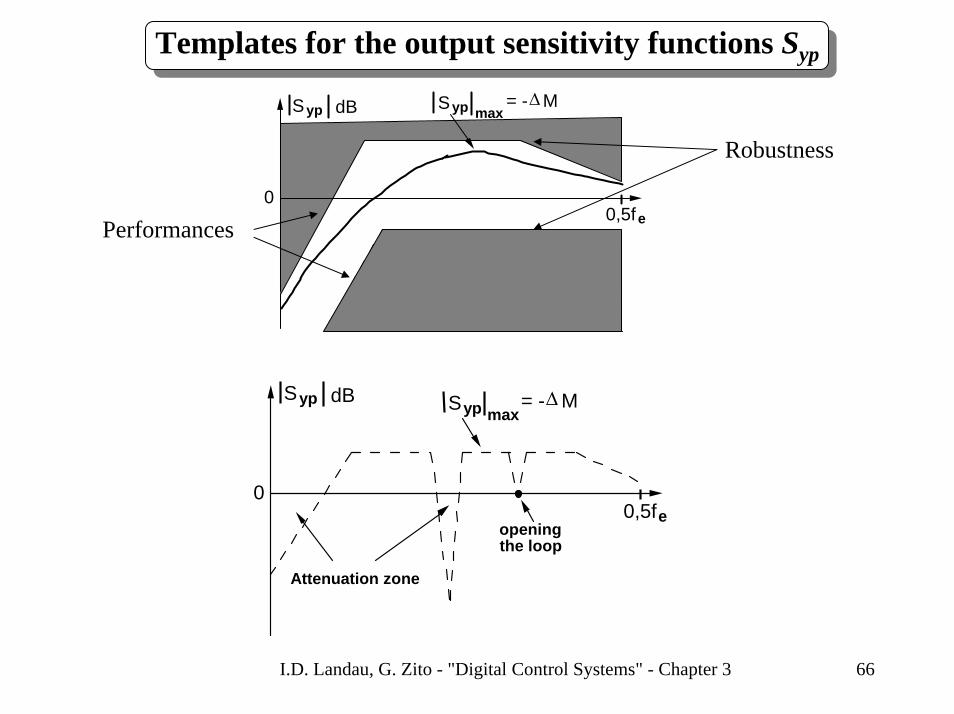
Templates for the output sensitivity functions Syp
Syp dB
0,5fe
Syp max= - M∆
0
Robustness
Performances
Syp dB
0,5fe
Syp max= - M∆
0
Attenuation zone
openingthe loop
I.D. Landau, G. Zito - "Digital Control Systems" - Chapter 3 67
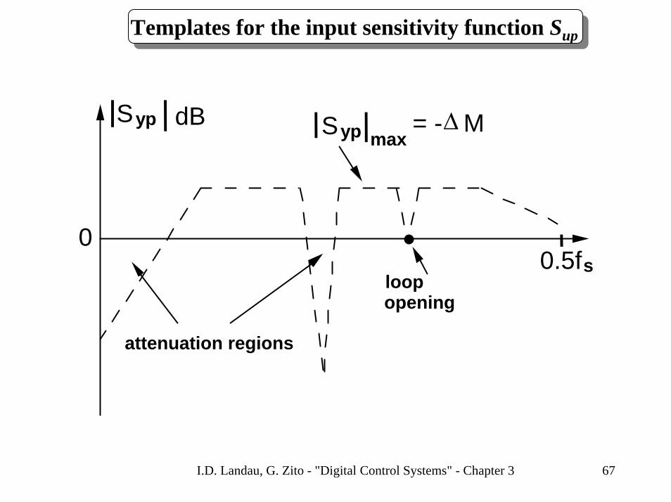
Templates for the input sensitivity function Sup
S yp dB
0.5fs
Syp max= - M∆
0
attenuation regions
loop opening
I.D. Landau, G. Zito - "Digital Control Systems" - Chapter 3 68
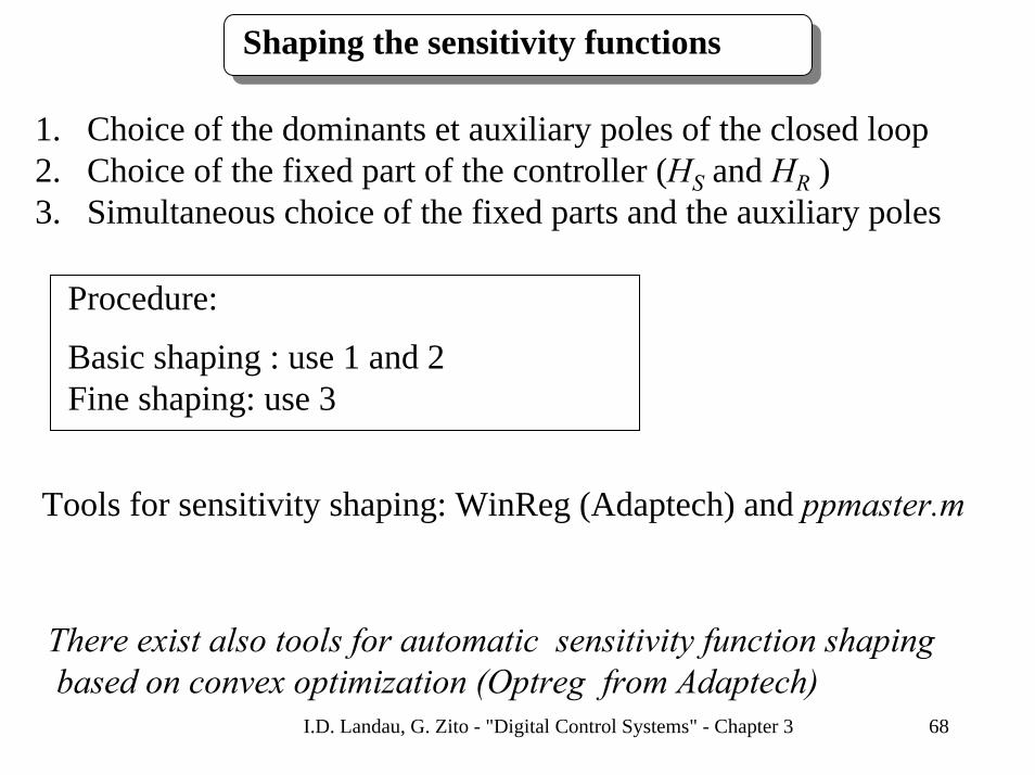
Shaping the sensitivity functions
1. Choice of the dominants et auxiliary poles of the closed loop2. Choice of the fixed part of the controller (HS and HR )3. Simultaneous choice of the fixed parts and the auxiliary poles
Procedure:
Basic shaping : use 1 and 2Fine shaping: use 3
Tools for sensitivity shaping: WinReg (Adaptech) and ppmaster.m
There exist also tools for automatic sensitivity function shapingbased on convex optimization (Optreg from Adaptech)
I.D. Landau, G. Zito - "Digital Control Systems" - Chapter 3 69
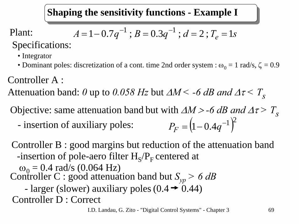
Shaping the sensitivity functions - Example I
Plant: sTdqBqA e 1;2;3.0;7.01 11 ===−= −−
Specifications:• Integrator• Dominant poles: discretization of a cont. time 2nd order system : ω0 = 1 rad/s, ζ = 0.9
Controller A :Attenuation band: 0 up to 0.058 Hz but ∆M < -6 dB and ∆τ < Ts
Objective: same attenuation band but with ∆M > -6 dB and ∆τ > Ts- insertion of auxiliary poles: ( )214.01 −−= qPF
Controller B : good margins but reduction of the attenuation band-insertion of pole-aero filter HS/PF centered at ω0 = 0.4 rad/s (0.064 Hz)
Controller C : good attenuation band but Syp > 6 dB - larger (slower) auxiliary poles (0.4 0.44)
Controller D : Correct

I.D. Landau, G. Zito - "Digital Control Systems" - Chapter 3 70
Shaping the sensitivity functions - Example I
0 0.05 0.1 0.15 0.2 0.25 0.3 0.35 0.4 0.45 0.5-25
-20
-15
-10
-5
0
5
10Syp Magnitude Frequency Responses
Frequency (f/fs)
Mag
nitu
de (d
B)
ABCDTemplate for Modulus marginTemplate for Delay margin = Ts

I.D. Landau, G. Zito - "Digital Control Systems" - Chapter 3 71
Shaping the sensitivity functions - Example II
Plant (integrator): sTdqBqA s 1;2;5.0;1 11 ===−= −−
q-dBA
u(t) y(t)
Sinusoidal disturbance (0.25 Hz)
Low frequencies disturbances
+
+
+
Specifications:1. No attenuation of the sinusoidal disturbance at (0.25 Hz)2. Attenuation band at low frequencies : 0 à 0.03 Hz3. Disturbances amplification at 0.07 Hz: < 3dB 4. Modulus margin > -6 dB and Delay margin > T5. No integrator in the controller

I.D. Landau, G. Zito - "Digital Control Systems" - Chapter 3 72
Shaping the sensitivity functions - Example II
1;1 2 =+= −SR HqH
Opening the loop at 0.25 Hz
- Fixed parts design :
-Dominant poles: discretization of a cont. time 2nd order system:ω0 = 0.628 rad/s, ζ = 0.9
Controller A : the specs. at 0.07 Hz are not fulfilled- insertion of a pole-zero filter HS/PF centered at ω0 = 0.44 rad/s
Controller B : Attenuation band smaller than that specified- dominant poles acceleration: ω0 = 0.9 rad/s
Controller C : Correct

I.D. Landau, G. Zito - "Digital Control Systems" - Chapter 3 73
Shaping the sensitivity functions - Example II
0 0.05 0.1 0.15 0.2 0.25 0.3 0.35 0.4 0.45 0.5-15
-10
-5
0
5
10Syp Magnitude Frequency Responses
Frequency (f/fs)
Mag
nitu
de (d
B)
ABCTemplate for Modulus marginTemplate for Delay margin = Ts

I.D. Landau, G. Zito - "Digital Control Systems" - Chapter 3 74
Some concluding remarks
• All the digital controllers has a three branches structure(R-S-T).• They have two degrees of freedom (tracking and regulation)• Controller design is done in two steps:
1) R et S (regulation) 2) T (tracking) • Controller complexity depends upon the plant model complexity• Pole placement is the basic control strategy• Tracking and regulation with independent objectives is applicable
to discrete time models with stable zeros• Internal model control is applicable only to stable and well
damped plants • Design of digital PID is a particular case of pole placement. Can
be used for the control of simple plants (order max. = 2)• All the digital controllers presented implement a predictive control
and they contain implicitly a predicition model of the plant