robust estimation for boundary correction in wavelet regression

This article was downloaded by: [Duke University Medical Center]On: 06 October 2014, At: 08:19Publisher: Taylor & FrancisInforma Ltd Registered in England and Wales Registered Number: 1072954 Registeredoffice: Mortimer House, 37-41 Mortimer Street, London W1T 3JH, UK

Journal of Statistical Computation andSimulationPublication details, including instructions for authors andsubscription information:http://www.tandfonline.com/loi/gscs20

Robust estimation for boundarycorrection in wavelet regressionAlsaidi M. Altaher a & Mohd Tahir Ismail aa School of Mathematical Sciences , Universiti Sains Malaysia ,11800 , Penang , MalaysiaPublished online: 05 Jul 2011.

To cite this article: Alsaidi M. Altaher & Mohd Tahir Ismail (2012) Robust estimation for boundarycorrection in wavelet regression, Journal of Statistical Computation and Simulation, 82:10,1531-1544, DOI: 10.1080/00949655.2011.585427

To link to this article: http://dx.doi.org/10.1080/00949655.2011.585427

PLEASE SCROLL DOWN FOR ARTICLE

Taylor & Francis makes every effort to ensure the accuracy of all the information (the“Content”) contained in the publications on our platform. However, Taylor & Francis,our agents, and our licensors make no representations or warranties whatsoever as tothe accuracy, completeness, or suitability for any purpose of the Content. Any opinionsand views expressed in this publication are the opinions and views of the authors,and are not the views of or endorsed by Taylor & Francis. The accuracy of the Contentshould not be relied upon and should be independently verified with primary sourcesof information. Taylor and Francis shall not be liable for any losses, actions, claims,proceedings, demands, costs, expenses, damages, and other liabilities whatsoever orhowsoever caused arising directly or indirectly in connection with, in relation to or arisingout of the use of the Content.

This article may be used for research, teaching, and private study purposes. Anysubstantial or systematic reproduction, redistribution, reselling, loan, sub-licensing,systematic supply, or distribution in any form to anyone is expressly forbidden. Terms &Conditions of access and use can be found at http://www.tandfonline.com/page/terms-and-conditions

http://www.tandfonline.com/loi/gscs20

http://www.tandfonline.com/action/showCitFormats?doi=10.1080/00949655.2011.585427

http://dx.doi.org/10.1080/00949655.2011.585427

http://www.tandfonline.com/page/terms-and-conditions

http://www.tandfonline.com/page/terms-and-conditions

Journal of Statistical Computation and SimulationVol. 83, No. 10, October 2012, 1531–1544

Robust estimation for boundary correction in wavelet regression

Alsaidi M. Altaher* and Mohd Tahir Ismail

School of Mathematical Sciences, Universiti Sains Malaysia, 11800, Penang, Malaysia

(Received 26 November 2010; final version received 29 April 2011 )

For boundary problems present in wavelet regression, two common methods are usually considered: poly-nomial wavelet regression (PWR) and hybrid local polynomial wavelet regression (LPWR). Normalityassumption played a key role for making such choices for the order of the low-order polynomial, thewavelet thresholding value and other calculations involved in LPWR. However, in practice, the normalityassumption may not be valid. In this paper, for PWR, we propose three automatic robust methods based on:MM-estimator, bootstrap and robust threshold procedure. For LPWR, the use of a robust local polynomial(RLP) estimator with a robust threshold procedure has been investigated. The proposed methods do notrequire any knowledge of noise distribution, are easy to implement and achieve high performances whenonly a small amount of data is in hand.A simulation study is conducted to assess the numerical performanceof the proposed methods.

Keywords: boundary region; MM-estimator; bootstrap; robust threshold; simulation.

Mathematics Subject Classification: 37M05; 62G35; 62G08; 65T60

1. Introduction

Suppose a noisy data set y1, y2, . . . , yn is observed from the fixed design model:

yi = f

(i

n

)+ εi, i = 1, 2, . . . , n = 2j , j = 1, 2, . . . , (1)

where f is an unknown function assumed to be a squared integral on the interval [0,1]. Thesequences {εi}ni=1 are independent and identically distributed normally with mean zero and aconstant variance, σ 2.

In this context, there is a variety of nonparametric techniques in the literature for estimating theunknown function, f , which allows for flexible modelling of the data. See, for example, booksby Eubank [1], Wahba [2] and Takezawa [3].

The past two decades have witnessed a great development of wavelet methods for estimatingan unknown function observed in the presence of noise, beginning from the seminal papers ofDonoho and Johnstone [4,5], where the concept of wavelet regression has been introduced in thestatistical literature.

*Corresponding author. Email: [email protected]

ISSN 0094-9655 print/ISSN 1563-5163 online© 2012 Taylor & Francishttp://dx.doi.org/10.1080/00949655.2011.585427http://www.tandfonline.com

Dow

nloa

ded

by [

Duk

e U

nive

rsity

Med

ical

Cen

ter]

at 0

8:19

06

Oct

ober

201

4

1532 A.M. Altaher and M.T. Ismail

In fact, wavelet regression possesses some key advantages which make it superior to traditionalnonparametric regression methods. It can be viewed as orthonormal basis functions that arelocalized in both time and frequency, with time-widths adapted to their frequency. Besides, it hasthe advantages of ideal minimax property, spatial inhomogeneous adaptivity and can be extendedto high dimension with fast algorithm.

However, wavelet regression has been proved to be highly effective in estimating the unknownfunction f as long as there are no boundary problems with f . Within boundaries, a partial datainformation is available due to the bounded support of the underlying function. As a result,the application of the wavelet transformation to a finite signal provides large biases at the edgesincreasing the bias, creating artificial wiggles. This problem has been recognized as a quite seriousone for easily getting boosted and substantially distorting the final estimates.

It is no doubt that in so many situations of our daily lives, we will be confronted by boundaryproblems, say, for instance, if we are interested in poverty data analysis, then it is necessaryto get reliable estimates of the income distribution on the left side, close to ‘0’ (left boundarypoint). Similarly, when using wavelet regression in econometrics, looking at the performance ofespecially old or young people, comparing large and small companies, etc., we always focus onthe boundaries estimates. For this, the boundary problem must be taken seriously.

Indeed, the boundary effects have been taken into account when using classical waveletregression by imposing on f some boundary assumptions such as symmetry or periodicity. Unfor-tunately, such assumptions are not always met and the problem still exists for some cases. As atreatment to this problem, Oh et al. [6] introduced a simple method in which the function f isdecomposed into a combination of wavelet regression function, fW(x), and a low-order polyno-mial model, fp(x), hoping to take the boundary problem into consideration by the polynomialmodel, which is well known for handling the boundary problem automatically. The progress ofa PWR involves two steps. First step is to regress the observed data {yi}ni=1 on {x, . . . , xd} for afixed order, d. The second step is to apply the wavelet regression to residuals {ei = yi − fp(x)}ni=1

to get fW (x). The final estimate of f , fPW will be the summation of fp(x) and fW (x). In fact, thecorrect order for a polynomial model would enable the polynomial estimator to remove the ‘non-periodicity’ in data. Then, the remaining signal can be well estimated using wavelet regressionwith, say, a periodic boundary assumption.

Different approaches have been proposed in order to find such choices of a proper polyno-mial order and threshold value. For a threshold value, perhaps the EBayesThresh procedure ofJohnstone and Silverman [7] is the most popular due to its good theoretical properties and goodperformance in simulations and in practice. On the other hand, several criteria have been pro-posed for selecting the correct order. We shall give a brief description of these approaches inSection 2.

We criticize the previous approaches from two points of view. First, ordinary least squares(OLS) is usually used to obtain the residuals at the first step. However, the OLS estimates caneasily be affected when the normality assumption is not met or in the presence of outliers, givinginaccurate estimates (see, for example, Maronna et al. [8]).

Second, the order selection criteria use functions of the residuals from all data to obtain theorder which minimizes the discrepancy between the predicted and true models. Normality of theresiduals again played a key role in deriving these criteria. The sensitivity of these estimationtechniques to these underlying assumptions has been identified as a weakness that can even leadto wrong interpretations.

Another method introduced by Oh and Lee [9] is used to cope with boundary problem. The ideais to combine wavelet regression with local polynomial regression, where the latter is well knownto possess excellent boundary properties. OLS is used for fitting the local polynomial model withEbayesThresh of Johnstone and Silverman [7]. Therefore, no robustness is taken into account;neither for the residuals at the first step nor for threshold values at the second step.

Dow

nloa

ded

by [

Duk

e U

nive

rsity

Med

ical

Cen

ter]

at 0

8:19

06

Oct

ober

201

4

Journal of Statistical Computation and Simulation 1533

(a) (b)

(c) (d)

(e) (f)

0.0 0.2 0.4 0.6 0.8 1.0 0.0 0.2 0.4 0.6 0.8 1.0

0.0 0.2 0.4 0.6 0.8 1.0 0.0 0.2 0.4 0.6 0.8 1.0

0.0 0.2 0.4 0.6 0.8 1.0 0.0 0.2 0.4 0.6 0.8 1.0

-10-5

05

10

-10-5

05

10

-10

-50

510

-10

-50

510

-10

-50

510

-10

-50

510

Figure 1. (a) The fit by robust estimation of Oh et al. [10]. (b) The fit by robust estimation of Oh et al. [11]. (c) The fitby classical polynomial wavelet regression. (d) The fit by classical LPWR. (e) The fit by robust PWR (proposed at 2.2).(f) The fit by robust LPWR (proposed at 2.4).

As a motivation, Figure 1 shows the fit of simulated data from HeavSine function [4] con-taminated with heavy noise from t-distribution with three degrees of freedom. The fit by robustestimation method of Oh et al. [10] in Figure 1(a) is smooth, but undersmoothing at the left bound-ary side and oversmoothing at the right boundary side. The fit by the robust estimation method ofOh et al. [11] is smooth at the middle, but wiggly undersmoothing at the left boundary side andwiggly oversmoothing at the right boundary side. The fit by classical PWR (Figure 1(c)) or LPWR(figure 1(d)) is sensitive to the outlier. In contrast, the fit at Figure 1(e) and (f) by our proposedmethods seems to balance between smoothness over the whole domain and outlier sensitivity.

Hence, in this paper, the main concern is to find an appropriate way to deal with the entireprocess of PWR and hybrid local polynomial wavelet shrinkage when the normality assumptionis not satisfied or in the presence of outliers.

In this regard, we propose four automatic robust methods. The first three methods are devotedfor PWR, while the other for classical LPWR:

1. We suggest using robust regression estimator instead of OLS; particularly, we shall use MM-estimator with the robust threshold procedure of Oh et al. [11].

2. We propose a new order selection criterion based on the bootstrap method by minimizing thepredicted mean-integrated squared error with a parametric penalty function, with the robustthreshold procedure of Oh et al. [11].

3. We suggest using OLS at the first step, but with the robust threshold procedure given by. Ohet al. [11].

4. For hybrid local polynomial wavelet shrinkage [9], we propose using the RLP estimator ofOh et al. [12], with the robust threshold procedure of Oh et al. [11].

The rest of this paper is organized as follows. In Section 2, we briefly review the two commonmethods for boundary correction in wavelet regression with a brief summary to some previous

Dow

nloa

ded

by [

Duk

e U

nive

rsity

Med

ical

Cen

ter]

at 0

8:19

06

Oct

ober

201

4


order selection criteria and their proposed threshold values for PWR. The proposed methods aredescribed in Section 3. Section 4 examines the practical performance of the proposed methodsvia a simulation study. A discussion is presented in Section 5.

2. Backround: boundary correction for wavelet regression

2.1. Polynomial wavelet regression

Let φ and ψ be father (scaling) and mother (dilation) wavelet functions, respectively, and thefunction f can be written in terms of wavelets as

fW (x) =∞∑

k=1

c0,kφk(x) +j−1∑j=0

2j −1∑k=1

dsj,kψj,k(x), (2)

where φk(x) = 21/2φ(2x − k), ψj,k(x) = 21/2ψ(2x − k), c0,k = ∑yiφk(xi) and ds

j,k denotes thesoft threshold coefficient.

Given a wavelet coefficient dj,k and a threshold value λ, the soft threshold rule, dsj,k , of the

coefficient can be defined as

dsj,k = sgn(dj,k)(|dj,k| − λ)I(|dj,k |>λ).

Here I refers to the usual indicator function. In other words, ‘soft’ means ‘to shrink or to kill’.Several methods were proposed to select an appropriate threshold value, λ, such as the Universal

of Donoho and Johnstone [4], Cross-Validation of Nason [13] and EbayesThresh of Johnstoneand Silverman [7]. A general review about some thresholding selection methods can be found inAbramovich et al. [14].

PWR method considered by Oh et al. [6] is basically based on a combination of waveletfunctions fW (x) and low-order polynomials fp(x). Therefore, the estimator of f , fPW is writtenas

fPW(x) = fp(x) + fW (x). (3)

To find fPW (x), it is proposed to regress the observed data {yi}ni=1 on {x1, x2, . . . , xd} for a fixed-order value, d Once fp(x) is estimated, the remaining signal is expected to be hidden in theresiduals, {ei = yi − fp(x)}ni=1. For this reason, the second step is to apply wavelet regressionusing Equation (2) for {ei}ni=1. The final estimate of f will be the summation of fp(x) and fW (x)

as in Equation (3). For more details, see [6] or [15].The use of PWR for resolving boundary problems works efficiently if the polynomial estimator

fp is able to remove the ‘non-periodicity’ in data and this certainly requires a correct order with anappropriate threshold to be used. In fact, different criteria have been proposed to aid in choosingthe order of the polynomial model that should be incorporated into wavelet functions in order toget successful corrections to the bias at the boundary region. Here, we give a brief introductionto the common ones.

Lee and Oh [15] propose two criteria. The first one is similar to Mallows’ [16]. It considers thevalue of d that maximizes r(d)

r(d) =d∑

i=1

a2i − 2σ 2d

n, d = 0, 1, . . . (4)

In this method, a model of order d should be used with SURE threshold.

Dow

nloa

ded

by [

Duk

e U

nive

rsity

Med

ical

Cen

ter]

at 0

8:19

06

Oct

ober

201

4


The second criterion is based on Bayesian information criterion (BIC) [17], which is employedto select d by minimizing BIC:

BIC = n log

[1

n

{n∑

i=1

yu − fp

}]+ d log(n), (5)

where {ai}di=0 represent the coefficients of the polynomial model.In this method, a model of order d was used with EbayeThresh of Johnstone and Silverman

[18]. However, for better performance another version of EbayeThresh introduced by Johnstoneand Silverman [7] can be used.

Oh and Kim [19] proposed three different Bayesian methods based on integrated likelihood,conditional empirical Bayes and reversible jump Markov chain Monte Carlo (MCMC). Formathematical details regarding these methods, see [19].

2.2. Hybrid local polynomial wavelet shrinkage

This method was introduced by Oh and Lee [9] as an improvement boundary adjustment in waveletregression. Instead of using the global polynomial fit, fp, it was proposed using a local polynomialfit fLp, Therefore, we can rewrite Equation (3) as

fH (x) = fLp(x) + fW (x),

where fH (x) is the hybrid local polynomial wavelet shrinkage estimator. fH (x) is computedthrough an iterative algorithm inspired by the back-fitting algorithm of Hastie and Tibshirani[20], see [9] for details.

3. The proposed methods

The following four sections describe our four automatic robust methods for boundary correctionin wavelet regression when the normality assumption is not met or in the presence of outliers.The first three methods are for polynomial regression whereas the last method is for hybridLPWR.

3.1. A method based on MM-estimator and robust threshold

This method is a two-stage procedure for selecting d and λ that minimizes the risk between f

and fPW. At the first stage, we apply the MM-estimator to estimate polynomial model param-eters to get fp(x). The polynomial order is selected as in Equation (5). At the second stage,we apply the classical wavelet regression to the residuals {ei = yi − fp(x)}ni=1 to get fW (x);with a soft threshold rule and a robust estimation process for λ as described in Oh et al. [11].The final estimate of f is fPW as in Equation (3). For complete details and mathematicaldescriptions of MM-estimator, refer to [21] and Maronna et al. [8]. Here, we point out thatwe compute MM-regression estimator as described in [21]. We use a bisquare re-descendingscore function that devotes to return a highly robust and highly efficient estimator (with 50%breakdown point and 95% asymptotic efficiency for normal errors). The S-estimator is computedusing the Fast-S algorithm of [22]. Standard errors are computed using the formulas of Crouxet al. [23].

Dow

nloa

ded

by [

Duk

e U

nive

rsity

Med

ical

Cen

ter]

at 0

8:19

06

Oct

ober

201

4


3.2. A method based on MM-estimator-bootstrap and robust threshold

Bootstrap has been shown to be a powerful tool because it requires less assumptions. It can also beapplied in an automatic way when a small set of data is available and standard methods invokingthe central limit theorem are inapplicable; see Shao [24] in the regression context.

However, our second method is also a two-stage procedure. First, we find fp(x) using theMM-estimator instead of OLS. In this method, the polynomial order is selected according to abootstrap criterion. We consider the order that minimizes the squared prediction error by addinga parametric penalty function. Secondly, we apply classical wavelet regression to the residuals{ei = yi − fp(x)}ni=1 to get fW (x) with a soft threshold rule and the robust threshold of Ohet al. [11]. The final estimate of f is fPW as in Equation (3).

The basic idea behind our bootstrap criterion for order selection is to generate a large numberof sub-samples by randomly drawing observations with replacement from the original data set ofresiduals. These sub-samples are then considered as bootstrap samples which would be used torecalculate the estimates of the standard error of predicted. Here, we summarize the key points ofour proposed method:

Repeat the following steps for d = 0, 1, . . . , dmax .Step 1: For a fixed value d , use the MM-estimator to regress {yi}ni=1 on {x, . . . , xd} for all theoriginal sample of observations to get the residuals {ei = yi − yi}ni=1.Step 2: Form {ei}ni=1 by inflating the {ei}ni=1 by the penalty function,

√1 − hi to ensure that

all residuals {ei}ni=1 have a constant variance. Here hi refers to the ith diagonal element of theprojection or hat matrix, H = X(X′X)−1X′.Step 3: Form a bootstrap pseudo-sample, {e∗

i }ni=1, by selecting with replacement from {ei}ni=1,then attached to {yi}ni=1 get a fixed-bootstrap values {y∗

i }ni=1, where y∗i = yi + e∗

i .Step 4: Apply MM-estimation for {y∗

i }ni=1 on {x, . . . , xd}. Let vi be the new residuals and thencompute the standard error of predicted νi say se∗(νi, d).Step 5: Repeat steps 3 and 4 for times to get se∗

1(νi, d), se∗2(νi, d), . . . , se∗

B(νi, d), then find theaverage of these estimates of the standard error of predicted say se∗(νi, d). Choose d that hasminimum se∗(νi, d).

There is no consensus agreement among statisticians on replication bootstrap number, B, andthe maximum polynomial order that should be used. However, for the replication number B, itis usually in the range 25–250 for estimating the standard error, while for bootstrap confidenceintervals, a much larger value of B is required, normally in the range 500–10,000. See, McQuarrieand Tsai [25], Imon andAli [26] or Uraibi et al. [27]. For Lee and Oh [15] used and Oh and Kim [19]used dmax = 4. In general, the polynomial order has to be smaller than the number of vanishingmoments, [6]. In our application, we shall use a coiflet with five vanishing moments and dmax = 4.

3.3. A method based on OLS with robust threshold (OLSR)

This method is similar to the methods explained above, in that it is a two-stage procedure. Unlikethe first two methods, the effect of non-normality assumption or outliers will be taken into accountat the second stage. That is, first, we employ the formula (5) to select the polynomial order andthen fp(x) using OLS. At the second step, we apply classical wavelet regression to the residuals{ei = yi − fp(x)}ni=1 to get fW (x) with the robust threshold value of Oh et al. [11]. The finalestimate of f is fPW as in Equation (3).

Dow

nloa

ded

by [

Duk

e U

nive

rsity

Med

ical

Cen

ter]

at 0

8:19

06

Oct

ober

201

4


3.4. Method based on robust local polynomial with robust threshold

In this method, at the first step, instead of using the global polynomial fit, fp, we shall use alocal polynomial fit. In fact, this idea has been used by Oh and Lee [9], where the normalityassumption and classical local polynomial fitting were considered. However, the aim here is totake into consideration the unsatisfied underlying assumption by using a RLP estimation insteadof the classical one. We shall use the RLP estimator of Oh et al. [12] which is based on M-typelocal polynomial using the concept of pseudo data. This estimator is easy to implement, and thealgorithm involved does not require any complex nonlinear optimization, with fast computation.Details can be found in [12].

Following Oh and Lee [9], we can use the following steps to find the final RLP wavelet regressionfitting (fRLPW):

1. Select an initial estimate f0 for f and let fRLP = f0.2. For j = 1, 2, . . ., iterate the following steps:a. Apply wavelet regression to the residuals yi − fRLP and obtain f

j

W .b. Estimate f

j

RLP by fitting the RLP regression to yi − fj

W .3. Stop if fRLPW = f

j

RLP + fj

W converges.

Before closing this subsection, we refer that the initial estimate, f0, can be found using Friedman’s(known as supsmu, available in R), while smoothing parameter is selected by a direct Plug-incriterion (available at KernSmooth package in R). Robust procedure of Oh et al. [11] is usedfor wavelet estimation at the second step with standard normal distribution function as a kernelfunction.

3.5. Other approaches

We have also considered some other combinations such as using EbayesThresh of Johnstone andSilverman [7] and robust estimation of Oh et al. [10] as an alternative to the robust thresholdprocedure of Oh et al. [11] when the boundary assumption is not satisfied. Another investigationincluded non-RLP with a robust threshold. However, the practical achievement of these approachesis inferior to our four suggested methods.

4. Simulation study

4.1. Setup

In this section, we have used the codes of the R statistical package to perform a simulation studyto assess the achievement of proposed methods comparing with the existing ones.

• ‘I’: Classical wavelet regression with robust estimation of [10].• ‘II’: Classical wavelet regression with robust estimation of [11].• ‘III’: PWR with robust threshold of [11] as described in Section 3.3 (robustness only for λ).• ‘IV’: PWR as described in Section 3.1 (robustness for both d, λ).• ‘V’: PWR as described in Section 3.2 with B = 30 (robustness for both d, λ).• ‘VI’: hybrid LPWR with robust threshold of Oh et al. [11] (robustness only for λ).• ‘VII’ hybrid LPWR as described in Section 3.4.

Throughout the whole simulation we used a maximal value of d = 4 for the polynomial model,whereas a coiflet with five vanishing moments and the periodic boundary assumption were used

Dow

nloa

ded

by [

Duk

e U

nive

rsity

Med

ical

Cen

ter]

at 0

8:19

06

Oct

ober

201

4


Table 1. The four functions used in simulation.

Test function Formula

1 Blocks of Donoho and Johnstone [4]2 Doppler of Donoho and Johnstone [4]3 (x − 0.8)ˆ2 + Blocks4 −(x − 0.3)ˆ2 + doppler

Test Function.1 Test Function.2

Test Function.3

0.0 0.2 0.4 0.6 0.8 1.0

-0.2

0.0

0.2

0.4

0.6

0.0 0.2 0.4 0.6 0.8 1.0-0

.2-0

.10.

00.

10.

2

0.0 0.2 0.4 0.6 0.8 1.0

0.0

0.2

0.4

0.6

0.8

1.0

0.0 0.2 0.4 0.6 0.8 1.0

-0.5

-0.3

-0.1

0.0

0.1

0.2

Test Function.4

Figure 2. The four test functions used in simulation.

for fW (x) as in [19]. Mother wavelet was N = 6 was used in every wavelet transform. Softthresholding was used for every method. The median absolute deviation of the wavelet coefficientsat the finest level was used to find variances for EbayesThresh. Laplace density and the medianof posterior were used for EbayesThresh.

Altogether four test functions were used. They are listed in Table 1 and are depicted in Figure 2.It is reasonable to assume functions 1 and 2 as periodic, while the remaining as a non-periodiccase. Four different kinds of noise were used:

• Pure Gaussian noise with mean zero and constant variance.• Heavy tail noise: from t-distribution with three degrees of freedom.• 10% contaminated normal mixture distribution: 0.9N(0, σ 2

snr=7 + 0.1N(0, σ 2snr=7/4)).• Correlated noises from AR(1): first-order autoregressive model with parameter (0.5).

Three levels of signal to noise ratio (snr) were used: snr = 3, 7 and 10. We consider two differentsample sizes: n = 64 and 128. For every combination of test function, noise structure, levelto noise level and sample size, 100 samples were generated. For each generated data set, weapplied the above seven methods to obtain an estimate (f ) for each test function (f ) and then themean-squared error was computed to be used as a numerical measure for assessing the qualityof f

MSE(f ) = 1

n

n∑i=1

[f

(i

n

)− f

(i

n

)]2

. (6)

Figures 2–5 display the box plot of the values of MSE(f ) for all test functions listed in Table 1 for(n = 128, snr = 3). As a part of our assessment for the seven wavelet methods, we apply paired

Dow

nloa

ded

by [

Duk

e U

nive

rsity

Med

ical

Cen

ter]

at 0

8:19

06

Oct

ober

201

4



Test Function.3

1 2 3 4 5 6 7 1 2 3 4 5 6 7

1 2 3 4 5 6 7 1 2 3 4 5 6 7

0.00

0.02

0.04

0.06

0.00

20.

004

0.00

60.

008

0.01

0

0.00

0.05

0.10

0.15

0.00

00.

005

0.01

00.

015

0.02

00.

025

Test Function.4

Figure 3. Box plot of MSE(f ) from simulation study, snr = 3, n = 128 and Gaussian noises.



1 2 3 4 5 6 7

0.00

0.02

0.04

0.06

1 2 3 4 5 6 7

0.00

20.

006

0.01

0

1 2 3 4 5 6 7

0.00

0.05

0.10

0.15

1 2 3 4 5 6 70.00

00.

010

0.02

0

Figure 4. Box plot of MSE(f ) from simulation study, snr = 3, n = 128 and mixture normal noises.

Wilcoxon tests to test whether the difference between the median of MSE(f ) values of any twowavelet methods is significant. The significance level was 1.25%. See [28], [15] or [19].

Tables 2–5 report the relative rankings of the median MSE(f ) for the seven used methods. Ifthe median MSE(f ) value of a certain method is significantly less than the remaining six methods,then it will be given rank ‘1’. If the median MSE(f ) value of a method is significantly larger thanonly one method but at the same time it is less than the five other methods, it will be assignedrank ‘2’, and similarly for ranks 3–7. However, if the median MSE values of the methods arenon-significant, then the same averaged rank is assigned. Other results were similar and henceomitted.

Since the boundary problem usually appears locally, the mean-squared error defined inEquation (6) may not measure the estimation equality properly. To have an idea of how theseven methods perform near the boundaries, we have calculated the mean squared error for the

Dow

nloa

ded

by [

Duk

e U

nive

rsity

Med

ical

Cen

ter]

at 0

8:19

06

Oct

ober

201

4


Test Function.1

0.00

0

Test Function.2

Test Function.3

1 2 3 4 5 6 7

0.00

0.02

0.04

0.06

1 2 3 4 5 6 7

0.00

20.

004

0.00

60.

008

0.01

01 2 3 4 5 6 7

0.00

0.05

0.10

0.15

1 2 3 4 5 6 70.

0000

.005

0.01

0 0.0

150.

0200

.025

Test Function.4

Figure 5. Box plot of MSE(f ) from simulation study, snr = 3, n = 128 and heavy noises from t(3).

Table 2. Pairwise Wilcoxon test rankings, for snr = 3, N = 128, Gaussian noises for theseven wavelet regression methods.

Method

Test function I II III IV V VI VII

1 7 6 2 2 2 4.5 4.52 7 6 4 4 4 1.5 1.53 7 6 2 4.5 4.5 2 24 7 6 3 3 3 3 3

Average rank 7 6 2.75 3.375 3.375 2.75 2.75

Table 3. Pairwise Wilcoxon test rankings, for snr = 3, N = 128, mixture normal noises forthe seven wavelet regression methods.

Method


1 7 6 1 4.5 4.5 2.5 2.52 7 6 3 3 3 3 33 7 6 3 3 3 3 34 7 6 3 3 3 3 3

Average rank 7 6 2.5 3.375 3.375 2.875 2.875

Table 4. Pairwise Wilcoxon test rankings, for snr = 3, N = 128, t (3) noises forthe seven wavelet regression methods.

Method


1 7 6 2 2 2 4.5 4.52 7 6 4 4 4 1.5 1.53 7 6 3 3 3 3 34 7 6 3 3 3 3 3

Average rank 7 6 3 3 3 3 3

Dow

nloa

ded

by [

Duk

e U

nive

rsity

Med

ical

Cen

ter]

at 0

8:19

06

Oct

ober

201

4


Table 5. Pairwise Wilcoxon test rankings, for snr = 3, N = 128, AR(1) noisesfor the seven wavelet regression methods.

Method


1 7 6 2 2 2 4.5 4.52 7 6 4 4 4 1.5 1.53 7 6 3 3 3 3 34 7 6 3 3 3 3 3

Average rank 7 6 3 3 3 3 3

Table 6. Simulation results of mean-squared error at the boundary region for the seven wavelet regression methods withsnr = 3, N = 128.

Method


1 0.009547 0.004683 0.001018 0.000867 0.000417 0.004148 0.0041482 0.002812 0.002030 0.001952 0.001539 0.001714 0.001055 0.0010553 0.161197 0.177071 0.001509 0.001452 0.001531 0.000487 0.0004874 0.088548 0.095359 0.001952 0.001851 0.001884 0.001107 0.001107

t (3) Noise1 0.009542 0.004784 0.001023 0.000815 0.000584 0.003992 0.0039922 0.002687 0.002041 0.001973 0.001322 0.001280 0.001030 0.0010303 0.162129 0.177401 0.001556 0.001321 0.001137 0.000670 0.0006704 0.089504 0.095483 0.001965 0.001504 0.001508 0.001056 0.001056

Mixture normal noise1 0.008546 0.006513 0.001702 0.001619 0.000707 0.003236 0.0032362 0.003210 0.002374 0.002587 0.002079 0.002045 0.001605 0.0016053 0.160323 0.174965 0.002307 0.001658 0.001346 0.000778 0.0007784 0.087637 0.094653 0.002582 0.002322 0.002173 0.001566 0.001566

AR(1) noise1 0.010451 0.005291 0.001460 0.001282 0.001131 0.004505 0.0045052 0.002888 0.002387 0.002189 0.001853 0.002001 0.001743 0.0017433 0.163037 0.180177 0.002151 0.001582 0.001486 0.001306 0.0013064 0.089766 0.096101 0.002246 0.001948 0.002072 0.001712 0.001712

Note: The values in bold refers to minimum value for mean squared error.

observations at the boundary region. Say [0, 0.05] ∪ [0.95, 1] as considered by Lee and Oh [15].In this case, the mean-squared error can be defined as

MSE(f ) = 1

n

∑i∈N(τ)

[f (xi) − f (xi)]2; τ = 1, 2, . . . ,n

2; xi = i

n,

where N(τ) = {1, . . . , τ, n − τ + 1, . . . , n}. Here τ refers to the number of observation at theboundary region for each side. In our case, since, n = 128, we have about seven observations ateach boundary side (τ = 7). Numerical results are reported in Table 6.

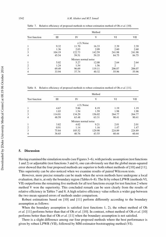
Finally, it is worth to end up by presenting numerical results to investigate the relative efficiencyof the four proposed methods relative to both robust estimations of [10] and [11] separately.Attention will be paid mainly to where the outliers are present. As a matter of fact, it is wellknown that noises from both mixture normal distribution and heavy tail distribution are goodexamples to investigate the robustness of outliers in our simulation study. Results are reported inTables 7 and 8.

Dow

nloa

ded

by [

Duk

e U

nive

rsity

Med

ical

Cen

ter]

at 0

8:19

06

Oct

ober

201

4


Table 7. Relative efficiency of proposed methods to robust estimation method of Oh et al. [10].

Method

Test function III IV V VI VII

t (3) Noise1 9.32 11.70 16.33 2.39 2.392 1.36 2.03 2.09 2.60 2.603 104.19 122.73 142.59 241.98 241.984 45.54 59.51 59.35 84.75 84.75

Mixture normal noise1 5.02 5.27 12.08 2.64 2.642 1.24 1.54 1.56 2 23 69.49 96.69 119.11 206.07 206.074 33.94 37.74 40.32 55.96 55.96

Table 8. Relative efficiency of proposed methods to robust estimation method of Oh et al. [11].

Method

Test function III IV V VI VII

t (3) Noise1 4.67 5.86 8.19 1.19 1.192 1.03 1.54 1.59 1.98 1.983 114.01 134.29 156.02 264.77 264.774 48.59 63.48 63.31 90.41 90.41

Mixture normal noise1 3.82 4.02 9.21 2.01 2.012 0.91 1.14 1.16 1.47 1.473 75.84 105.52 129.98 224.89 224.894 36.65 40.76 43.55 60.44 60.44

5. Discussion

Having examined the simulation results (see Figures 3–6), with periodic assumption (test functions1 and 2) or adjustable (test functions 3 and 4), one can obviously see that the global mean-squarederror showed that the four proposed methods are superior to both robust methods of [10] and [11].This superiority can be also noticed when we examine results of paired Wilcoxon tests.

However, more precise remarks can be made when the seven methods have undergone a localevaluation, that is, at only the boundary region (Tables 6–8). The fit by robust LPWR (methods VI,VII) outperforms the remaining five methods for all test functions except for test function 2 wheremethod V won the superiority. This concluded remark can be seen clearly from the results ofrelative efficiency in Tables 7 and 8. A high relative efficiency value reflects a wider gap betweenthe two mean squared errors of methods under comparison.

Robust estimations based on [10] and [11] perform differently according to the boundaryassumption as follows:

When the boundary assumption is satisfied (test functions 1, 2), the robust method of Ohet al. [11] performs better than that of Oh et al. [10]. In contrast, robust method of Oh et al. [10]performs better than that of Oh et al. [11] when the boundary assumption is not satisfied.

There is a slight difference among our four proposed methods where the best performance isgiven by robust LPWR (VII), followed by MM-estimator-bootstrapping method (VI).

Dow

nloa

ded

by [

Duk

e U

nive

rsity

Med

ical

Cen

ter]

at 0

8:19

06

Oct

ober

201

4



Test Function.3

1 2 3 4 5 6 7

0.00

0.02

0.04

0.06

1 2 3 4 5 6 7

0.00

20.

004

0.00

60.

008

0.01

01 2 3 4 5 6 7

0.00

0.05

0.10

0.15

1 2 3 4 5 6 70.

000

0.00

50.

010

0.01

50.

020

0.02

5

Test Function.4

Figure 6. Box plot of MSE(f ) from simulation study, snr = 3, n = 128 and noises from AR(1).

Overall, we can conclude that these simulation results seem to suggest that it is preferable tocorrect the boundary bias of wavelet regression as we recommended in Section 3. That is, whenthe normality assumption is not satisfied or in the presence of outliers.

Acknowledgment

This research is supported by Universiti Sains Malaysia.

References

[1] R.L. Eubank, Spline Smoothing and Nonparametric Regression, Marcel Dekker, New York, 1988.[2] G. Wahba, Spline Models for Observational Data, SIAM, Philadelphia, PA, 1990.[3] K. Takezawa, Introduction to Nonparametric Regression, John Wiley, Hoboken, NJ, 2006.[4] D.L. Donoho and I.M. Johnstone, Ideal spatial adaptation by wavelet shrinkage, Biometrika 81 (1994), pp. 425–455.[5] D.L. Donoho and I.M. Johnstone, Adapting to unknown smoothness via wavelet shrinkage, J. Amer. Statist. Assoc.

90(432) (1995), pp. 1200–1224.[6] H.S. Oh, P. Naveau, and G. Lee, Polynomial boundary treatment for wavelet regression, Biometrika 88 (2001), pp.

291–298.[7] I.M. Johnstone and B.W. Silverman, Empirical Bayes selection of wavelet thresholds, Ann. Statist. 33 (2005), pp.

1700–1752.[8] R. Maronna, R. Martin, and V. Yohai, Robust Statistics, Wiley, New York, 2006.[9] H.S. Oh and T.C.M. Lee, Hybrid local polynomial wavelet shrinkage: Wavelet regression with automatic boundary

adjustment, Comput. Statist. Data Anal. 48(4) (2005), pp. 809–820.[10] H.S. Oh, D.W. Nychka, and T.C.M. Lee, The role of pseudo data for robust smoothing with application to wavelet

regression, Biometrika 94 (2007), pp. 893–904.[11] H.S Oh, D. Kim, and Y. Kim, Robust wavelet shrinkage using robust selection of thresholds, Statist. Comput. 19(1)

(2009), pp. 27–34.[12] H.S. Oh, J. Lee, and D. Kim, A recipe for robust estimation using pseudo data, J. Korean Statist. Soc. 37(1) (2008),

pp. 63–72.[13] G.P. Nason, Wavelet shrinkage by cross-validation, Roy. Statist. Soc. B 58 (1996), pp. 463–479.[14] F. Abramovich, T.C. Bailey, and T. Sapatinas, Wavelet analysis and its statistical applications, The Statistician 49

(2000), pp. 1–29.[15] T. Lee and H.S. Oh, Automatic polynomial wavelet regression, Statist. Comput. 14 (2004), pp. 337–341.[16] C.L. Mallows, Some comments on Cp, Technometrics 15 (1973), pp. 661–675.[17] G. Schwarz, Estimating the dimension of a model, Ann. Statist. 6(2) (1978), pp. 461–464.[18] I.M. Johnstone and B.W. Silverman, Empirical Bayes selection of wavelet thresholds, unpublished manuscript (2003).

Dow

nloa

ded

by [

Duk

e U

nive

rsity

Med

ical

Cen

ter]

at 0

8:19

06

Oct

ober

201

4


[19] H.-S. Oh and H.-M. Kim, Bayesian automatic polynomial wavelet regression, J. Statist. Plann. Inference 138(8)(2008), pp. 2303–2312.

[20] T. Hastie and R. Tibshirani, Generalized Additive Models, Chapman & Hall, London, 1990.[21] V.J. Yohai, High breakdown-point and high efficiency robust estimates for regression, Ann. Statist. 15 (1987), pp.

642–656.[22] M. Salibian-Barrera and V.J. Yohai, A fast algorithm for S-regression estimates, J. Comput. Graph. Statist. 15(2)

(2006), pp. 414–427.[23] C. Croux, G. Dehaene, and D. Hoorelbeke, Robust standard errors for robust estimators, Discussion Papers Series

03.16, K.U. Leuven, 2003.[24] J. Shao, Bootstrap model selection, J. Amer. Statist. Assoc. 91(434) (1996), pp. 655–665.[25] A.D.R. McQuarrie and C.L. Tsai, Regression and Time Series Model Selection. World Scientific, Singapore, 1998.[26] A.H.M.R. Imon and M.M. Ali, Bootstrapping regression residuals, J. Korean Statist. Soc. 16 (2005), pp. 665–682.[27] H. Uraibi, H. Midi, B. Talib, and J.Yousif, Linear regression model selection based on robust bootstrapping technique,

Am. J. Appl. Sci. 6 (2009), pp. 1191–1198.[28] M.P. Wand, A comparison of regression spline smoothing procedures, Comput. Statist. 15 (2000), pp. 443–462.

Dow

nloa

ded

by [

Duk

e U

nive

rsity

Med

ical

Cen

ter]

at 0

8:19

06

Oct

ober

201

4

robust estimation for boundary correction in wavelet regression

Documents