robust loss development using mcmc: a...

Robust Loss Development Using MCMC: A Vignette

Christopher W. Laws Frank A. Schmid

July 2, 2010

Abstract

For many lines of insurance, the ultimate loss associated with a particular exposure (acci-dent or policy) year may not be realized (and hence known) for many calendar years; insteadthese losses develop as time progresses. The actuarial concept of loss development aims atestimating (at the level of the aggregate loss triangle) the ultimate loss by exposure year,given their respective stage of maturity (as defined by the time distance between the expo-sure year and the latest observed calendar year). This vignette describes and demonstratesloss development using of the package lossDev, which centers on a Bayesian time seriesmodel. Notable features of this model are a skewed Student-t distribution with time-varyingscale and skewness parameters, the use of an expert prior for the calendar year effect, andthe ability to accommodate a structural break in the consumption path of services. R andthe package are open-source software projects and can be freely downloaded from CRAN:http://cran.r-project.org and http://lossdev.r-forge.r-project.org/.

1 Installation

At the time of writing this vignette, the current version of lossDev is 0.9.3, which has beenreleased as an R package and can be downloaded from http://lossdev.r-forge.r-project.

org/. lossDev should be available on CRAN shortly. (For instructions on installing R packagesplease see the help files for R.) lossDev requires rjags for installation. rjags requires that avalid version of JAGS be installed on the system. JAGS is an open source program for analysis ofBayesian hierarchical models using Markov Chain Monte Carlo (MCMC) simulation and can befreely download from http://calvin.iarc.fr/~martyn/software/jags/.

2 Model Overview

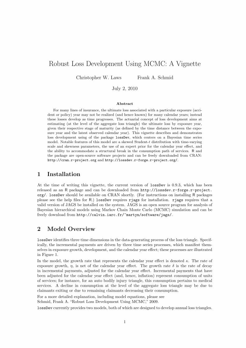
lossDev identifies three time dimensions in the data-generating process of the loss triangle. Specif-ically, the incremental payments are driven by three time series processes, which manifest them-selves in exposure growth, development, and the calendar year effect; these processes are illustratedin Figure 1.

In the model, the growth rate that represents the calendar year effect is denoted κ. The rate ofexposure growth, η, is net of the calendar year effect. The growth rate δ is the rate of decayin incremental payments, adjusted for the calendar year effect. Incremental payments that havebeen adjusted for the calendar year effect (and, hence, inflation) represent consumption of unitsof services; for instance, for an auto bodily injury triangle, this consumption pertains to medicalservices. A decline in consumption at the level of the aggregate loss triangle may be due toclaimants exiting or due to remaining claimants decreasing their consumption.

For a more detailed explanation, including model equations, please seeSchmid, Frank A. “Robust Loss Development Using MCMC,” 2009.

lossDev currently provides two models, both of which are designed to develop annual loss triangles.

1

http://cran.r-project.org

http://lossdev.r-forge.r-project.org/



http://calvin.iarc.fr/~martyn/software/jags/

Figure 1: Triangle Dynamics.

Section 3 uses the first (“standard”) model, which assumes that all exposure years are subject toa common consumption path.

Section 4 uses the second (“change point”) model to develop a loss triangle with a structural breakin the consumption path, thus assuming that earlier exposure years are subject to one consumptionpath and later exposure years are subject to another.

3 Using the Standard Model for Estimation

3.1 Data

The standard model (which does not allow for a structural break) is demonstrated on a loss trianglefrom Automatic Facilitative business in General Liability (excluding Asbestos & Environmental).The payments are on an incurred basis.

This triangle is taken fromMack, Thomas, “Which Stochastic Model is Underlying the Chain Ladder Method,”Casualty Ac-tuarial Society Forum, Fall 1995, pp. 229-240, http://www.casact.org/pubs/forum/95fforum/95ff229.pdf.

3.2 Model Specification

Standard models are specified with the function makeStandardAnnualInput. This function takesas input all data used in the estimation process. makeStandardAnnualInput also allows the userto vary the model specification through several arguments. Most of these arguments have defaultsthat should be suitable for most purposes.

To ensure portability, the data used in this vignette is packaged in lossDev and as such is loadedusing the data function. However, the user wishing to develop other loss triangles should loadthe data using standard R functions (such as read.table or read.csv). See the R manual forassistance.

3.2.1 Loading and Manipulating the Data

The Triangle As input, makeStandardAnnualInput can take either a cumulative loss triangleor an incremental loss triangle (or in the case where one might not be directly calculable fromthe other, both triangles may be supplied). makeStandardAnnualInput expects any supplied losstriangle to be a matrix. The row names for the matrix must be the Accident (or Policy) Year

2

http://www.casact.org/pubs/forum/95fforum/95ff229.pdf


and must appear in ascending order. The matrix must be square and all values below the latestobserved diagonal must be missing; missing values on and above this diagonal are permitted.

Note the negative value in Accident Year 1982 in the example triangle. Because incrementalpayments are modeled on the log scale, this value will be treated as missing, which could result ina slightly overstated ultimate loss. A comparison of predicted vs observed cumulative paymentsin Figure 9 indicates that, at least in this instance, this possible overstatement is not a concern.

> library(lossDev)

module basemod loaded

module bugs loaded

module lossDev loaded

> data(IncrementalGeneralLiablityTriangle)

> IncrementalGeneralLiablityTriangle <- as.matrix(IncrementalGeneralLiablityTriangle)

> print(IncrementalGeneralLiablityTriangle)

DevYear1 DevYear2 DevYear3 DevYear4 DevYear5 DevYear6 DevYear7 DevYear8

1981 5012 3257 2638 898 1734 2642 1828 599

1982 106 4179 1111 5270 3116 1817 -103 673

1983 3410 5582 4881 2268 2594 3479 649 603

1984 5655 5900 4211 5500 2159 2658 984 NA

1985 1092 8473 6271 6333 3786 225 NA NA

1986 1513 4932 5257 1233 2917 NA NA NA

1987 557 3463 6926 1368 NA NA NA NA

1988 1351 5596 6165 NA NA NA NA NA

1989 3133 2262 NA NA NA NA NA NA

1990 2063 NA NA NA NA NA NA NA

DevYear9 DevYear10

1981 54 172

1982 535 NA

1983 NA NA

1984 NA NA

1985 NA NA

1986 NA NA

1987 NA NA

1988 NA NA

1989 NA NA

1990 NA NA

The Stochastic Inflation Prior Incremental payments may be subject to inflation. One cansupply makeStandardAnnualInput with a price index, such as the CPI, as an expert prior for therate of inflation. The supplied rate of inflation must cover the years of the supplied incrementaltriangle and may extend (both into the past and future) beyond these years. If a future year’srate of inflation is needed but is yet unobserved, it will be simulated from an Ornstein–Uhlenbeckprocess that has been calibrated to the supplied inflation series.

For this example, the CPI is taken as a prior for the stochastic rate of inflation.

Note that observed rates of inflation that extend beyond the last observed diagonal in Incremen-

talGeneralLiablityTriangle are not utilized in this example, although lossDev is capable ofdoing so.

> data(CPI)

> CPI <- as.matrix(CPI)[, 1]

3

> CPI.rate <- CPI[-1]/CPI[-length(CPI)] - 1

> CPI.rate.length <- length(CPI.rate)

> print(CPI.rate[(-10):0 + CPI.rate.length])

1997 1998 1999 2000 2001 2002 2003

0.02294455 0.01557632 0.02208589 0.03361345 0.02845528 0.01581028 0.02279044

2004 2005 2006 2007

0.02663043 0.03388036 0.03225806 0.02848214

> CPI.years <- as.integer(names(CPI.rate))

> years.available <- CPI.years <= max(as.integer(dimnames(IncrementalGeneralLiablityTriangle)[[1]]))

> CPI.rate <- CPI.rate[years.available]

> CPI.rate.length <- length(CPI.rate)

> print(CPI.rate[(-10):0 + CPI.rate.length])

1980 1981 1982 1983 1984 1985 1986

0.13498623 0.10315534 0.06160616 0.03212435 0.04317269 0.03561116 0.01858736

1987 1988 1989 1990

0.03649635 0.04137324 0.04818259 0.05403226

3.2.2 Selection of Model Options

The function makeStandardAnnualInput has many options to allow for customization of modelspecification; however, not all options will be illustrated in this tutorial.

For this example, the loss history is supplied as incremental payments to the argument incremen-tal.payments. The exposure year type of this triangle is set to Accident Year by setting the valueof exp.year.type to “ay.” The default is “ambiguous” which should be sufficient in most cases asthis information is only utilized by a handful of functions and the information can be supplied (oroverridden calling those functions).

The function allows for the specification of two rates of inflation (in addition to a zero rate ofinflation). One of these rates is allowed to be stochastic, meaning that uncertainty in futurerates of this inflation series are simulated from a process calibrated to the observed series. Forthe current demonstration, it will be assumed that the CPI is the only applicable inflation rate,and that this rate is stochastic. This is done by setting the value of stoch.inflation.rate toCPI.rate (which was created earlier). The user has the option of specifying what percentage ofdollars inflate at stoch.inflation.rate, with this value being allowed to vary for each cell of thetriangle. For the current illustration, it is assumed that all dollars (in all periods) follow the CPI.This is done by setting stoch.inflation.weight to 1 and non.stoch.inflation.weight to 0.

By default, the measurement equation for the logarithm of the incremental payments is a Student-t. The user has the option of using a skewed-t by setting the value of use.skew.t to TRUE. Forthis demonstration, a skewed-t will be used.

Because lossDev is designed to develop loss triangles to ultimate, some assumptions must bemade with regard to the extension of the consumption path beyond the number of developmentyears in the observed triangle. The default assumes the last estimated decay rate (i.e., growthrate of consumption) is applicable for all future development years, and such is assumed for thisexample. This default can be overridden by the argument projected.rate.of.decay. Addition-ally, either the final number of (possibly) non-zero payments must be supplied via the argumenttotal.dev.years or the number of non-zero payments in addition to the number of developmentyears in the observed triangle must be supplied via the argument extra.dev.years. Similarly,the number of additional, projected exposure years can also be specified.

> standard.model.input <- makeStandardAnnualInput(incremental.payments = IncrementalGeneralLiablityTriangle,

+ stoch.inflation.weight = 1, non.stoch.inflation.weight = 0,

4

+ stoch.inflation.rate = CPI.rate, exp.year.type = "ay", extra.dev.years = 5,

+ use.skew.t = TRUE)

3.3 Estimating the Model

Once the model has been specified, it can be estimated.

MCMC Overview The model is Bayesian and estimated by means of Markov chain MonteCarlo Simulation (MCMC). To perform MCMC, a Markov chain is constructed in such a waythat the limiting distribution of the chain is the posterior distribution of interest. The chain isinitialized with starting values and then run until it has reached a point of convergence in whichsamples adequately represent random (albeit sequentially dependent) draws from this posteriordistribution. The set of iterations performed (and discarded) until samples are assumed to bedraws from the posterior is called a “burn-in.” After the burn-in, the chain is iterated further tocollect samples. The samples are then used to calculated the statistic of interest.

While the user is not responsible for the construction of the Markov chain, he is responsible forassessing the chains’ convergence. (Section 3.4.1 gives some pointers on this.) The most commonway of accomplishing this task is to run several chains simultaneously with each chain having beenstarted with a different set of initial values. Once all chains are producing similar results, one canassume that the chains have converged.

To estimate the model, the function runLossDevModel is called with the first argument beingthe input object created by makeStandardAnnualInput. To specify the number of iterations todiscard, the user sets the value of burnIn. To specify the number of iterations to perform after theburn-in, set the value of sampleSize. To set the number of chains to run simultaneously, supplya value for nChains. The default value for nChains is 3, which should be sufficient for most cases.

It is also common practice (due to possible autocorrelation in the samples) to apply “thining,”which means that only every n-th draw is stored. The argument thin is available for this purpose.

Memory Issues MCMC can require large amounts of memory. To allow lossDev to workwith limited hardware, the R package filehash is used to cache the codas of monitored valuesto the hard-drive in an efficient way. While such caching can allow estimation of large triangleson computers with limited memory, it can also slow down some computations. The user has theoption of turning this feature on and off. This is done via the function lossDevOptions by settingthe argument keepCodaOnDisk to TRUE or FALSE.

R also makes available the function memory.limit, which one may find useful.

> standard.model.output <- runLossDevModel(standard.model.input,

+ burnIn = 30000, sampleSize = 30000, thin = 10)

Compiling data graph

Resolving undeclared variables

Allocating nodes

Initializing

Reading data back into data table

Compiling model graph


Allocating nodes

Graph Size: 7388

[1] "Update took 16.7776 mins"

5

3.4 Examining Output

makeStandardAnnualInput returns a complex output object. lossDev provides several user-levelfunctions to access the information contained in this object. Many of these functions are describedbelow.

3.4.1 Assessing Convergence

As mentioned, the user is responsible for assessing the convergence of the Markov chains used toestimate the model. To this aim, lossDev provides several functions to produce trace and densityplots.

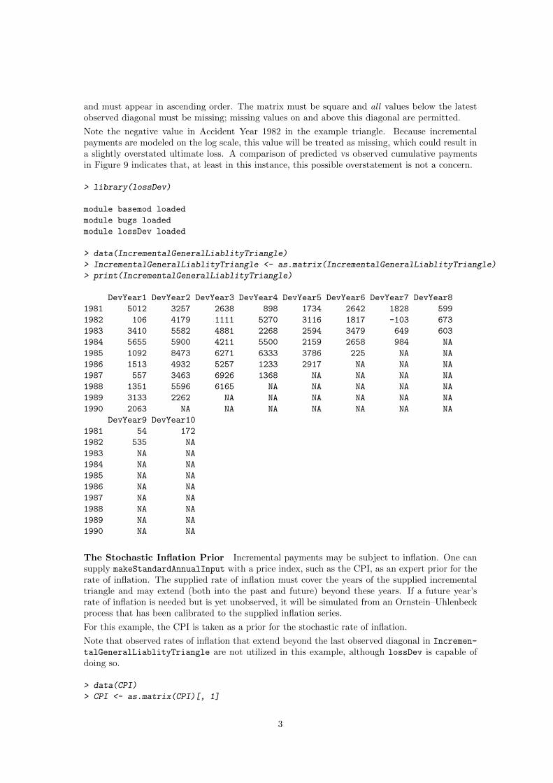
Arguably, the most important charts for assessing convergence are the trace plots associatedwith the three time dimensions of the model. Convergence of exposure growth, the consumptionpath, and the calendar year effect are assessed in Figures 2, 3, and 4 respectively. These chartsare produced with the functions exposureGrowthTracePlot, consumptionPathTracePlot, andcalendarYearEffectErrorTracePlot.

> exposureGrowthTracePlot(standard.model.output)

0 500 1000 1500 2000 2500 3000

−0.

50.

51.

5

Exposure Growth :2

Sample

Par

amet

er V

alue

0 500 1000 1500 2000 2500 3000

−0.

50.

5

Exposure Growth :6

Sample

Par

amet

er V

alue

0 500 1000 1500 2000 2500 3000

010

2030

Exposure Growth :11

Sample

Par

amet

er V

alue

Figure 2: Trace plots for select exposure growth parameters.

3.4.2 Assessing Model Fit

lossDev provides many diagnostic charts to asses how well the model fits the observed triangle.

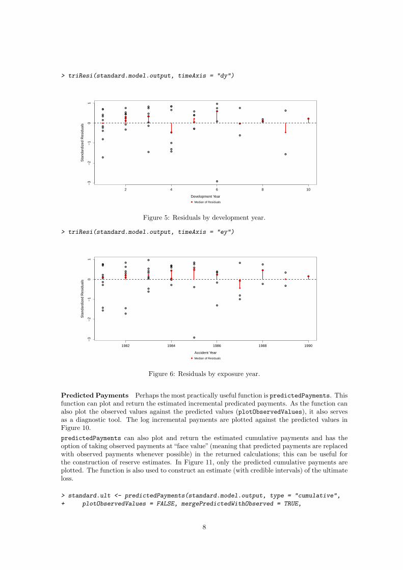
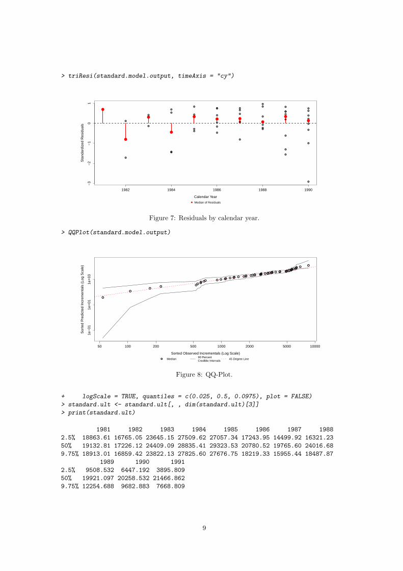
Residuals For the analysis of residuals, lossDev provides the function triResi. triResi plotsthe residuals (on the log scale) by the three time dimensions. The time dimension is selected bymeans of the argument timeAxis. By default, residual charts are standardized to account forany assumed/estimated heteroskedasticity in the (log) incremental payments. These charts canbe found in Figures 5, 6, and 7.

Note that because (the log) incremental payments are allowed to be skewed, the residuals neednot be symmetric.

QQ-Plot lossDev provides a QQ-Plot in the function QQPlot. QQPlot plots the median ofsimulated incremental payments (sorted at each simulation) against the observed incrementalpayments. Plotted points from a well calibrated model will be close to the 45-degree line. Theseresults are shown in Figure 8.

6

> consumptionPathTracePlot(standard.model.output)

0 500 1000 1500 2000 2500 3000

−0.

51.

02.

0

Calendar Year Effect Error :3

Sample

Par

amet

er V

alue

0 500 1000 1500 2000 2500 3000

01

23


Sample

Par

amet

er V

alue

0 500 1000 1500 2000 2500 3000

04

8


Sample

Par

amet

er V

alue

Figure 3: Trace plots for select development years on the consumption path.

> calendarYearEffectErrorTracePlot(standard.model.output)

0 500 1000 1500 2000 2500 3000

−0.

51.

02.

0


Sample

Par

amet

er V

alue

0 500 1000 1500 2000 2500 3000

01

23


Sample

Par

amet

er V

alue

0 500 1000 1500 2000 2500 3000

04

8


Sample

Par

amet

er V

alue

Figure 4: Trace plots for select calendar year effect errors.

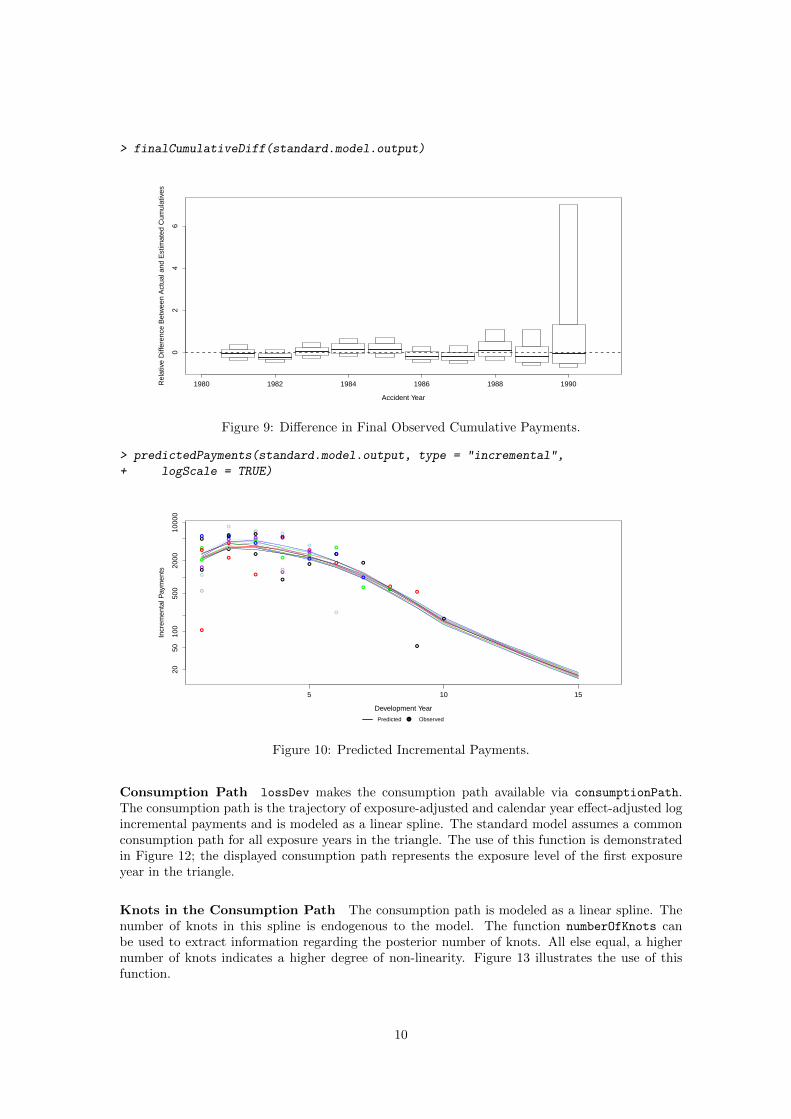
Comparison of Cumulative Payments As a means of assessing how well the predicted cu-mulative payments line up with the observed values, lossDev provides the function finalCu-

mulativeDiff. This function plots the relative difference between the predicted and observedcumulative payments (when such payments exists) for the last observed cumulative payment ineach exposure year, alongside credible intervals. These relative differences, which are shown inFigure 9, can be useful for assessing the impact of negative incremental payments, as discussed.

3.4.3 Extracting Inference and Results

After compiling, burning-in, and sampling, the user will wish to extract results from the output.Many of the functions mentioned in this section also return the values of some plotted information.These values are returned invisibly and as such are not printed at the REPL unless such anoperation is requested. Additionally, many of these functions also provide an option to suppressplotting.

7

> triResi(standard.model.output, timeAxis = "dy")

2 4 6 8 10

−3

−2

−1

01

Development Year

Sta

ndar

dize

d R

esid

uals

●

●

●

●

●

●

●

●

●

● ●

●

●●

●

●

●

●

●

●

●

●

●

●

●

●●

●

●

●

●

●

●

●

●

●

●

●

●

●

●

●

●

●

●

●

●

●●

●●

●

●

●

●

●●

●

●

●

●

●

●

●

● Median of Residuals

Figure 5: Residuals by development year.

> triResi(standard.model.output, timeAxis = "ey")

1982 1984 1986 1988 1990

−3

−2

−1

01

Accident Year

Sta

ndar

dize

d R

esid

uals

●

●

●

●

●

●●

●

●

●

●

●

●

●

●

●●

●

●

●

●

●

●

●

●

●

●

●

●

●

●

●

●

●

●

●

●

●

●

●

●●

●

●

●

●

●

●

●

●

●

●

●

●●

● ●

●

●

●

●

●

●

●


Figure 6: Residuals by exposure year.

Predicted Payments Perhaps the most practically useful function is predictedPayments. Thisfunction can plot and return the estimated incremental predicated payments. As the function canalso plot the observed values against the predicted values (plotObservedValues), it also servesas a diagnostic tool. The log incremental payments are plotted against the predicted values inFigure 10.

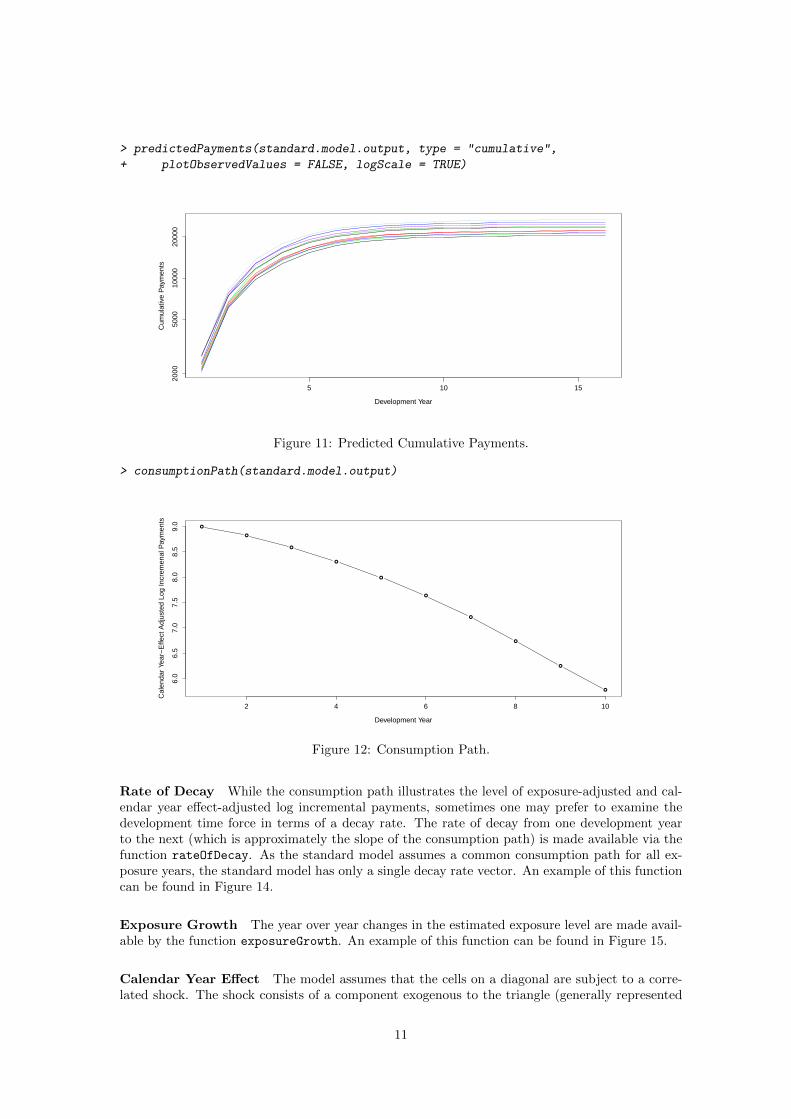
predictedPayments can also plot and return the estimated cumulative payments and has theoption of taking observed payments at “face value” (meaning that predicted payments are replacedwith observed payments whenever possible) in the returned calculations; this can be useful forthe construction of reserve estimates. In Figure 11, only the predicted cumulative payments areplotted. The function is also used to construct an estimate (with credible intervals) of the ultimateloss.

> standard.ult <- predictedPayments(standard.model.output, type = "cumulative",

+ plotObservedValues = FALSE, mergePredictedWithObserved = TRUE,

8

> triResi(standard.model.output, timeAxis = "cy")

1982 1984 1986 1988 1990

−3

−2

−1

01

Calendar Year

Sta

ndar

dize

d R

esid

uals

●●

●

●

●

●

●

●

●

●

●

●●

●●

●●

●

●

●

●

●

●

●

●

●

●

●

●

●

●

●●

●

●

●

●

●

●

●

●

●●

●

●

●

●

●●

●

●

●

●

●

●

●

●

●

●

●

●

●

●●


Figure 7: Residuals by calendar year.

> QQPlot(standard.model.output)

50 100 200 500 1000 2000 5000 10000

1e−

011e

+01

1e+

03

Sorted Observed Incrementals (Log Scale)

Sor

ted

Pre

dict

ed In

crem

enta

ls (

Log

Sca

le)

●

●●

●●

● ●●●● ● ● ●● ● ●● ● ●●● ●●●● ●●●● ● ●●●●●● ● ●● ●●●●●●●●●

●●●●●

●

● Median90 PercentCredible Intervals

45 Degree Line

Figure 8: QQ-Plot.

+ logScale = TRUE, quantiles = c(0.025, 0.5, 0.0975), plot = FALSE)

> standard.ult <- standard.ult[, , dim(standard.ult)[3]]

> print(standard.ult)

1981 1982 1983 1984 1985 1986 1987 1988

2.5% 18863.61 16765.05 23645.15 27509.62 27057.34 17243.95 14499.92 16321.23

50% 19132.81 17226.12 24409.09 28835.41 29323.53 20780.52 19765.60 24016.68

9.75% 18913.01 16859.42 23822.13 27825.60 27676.75 18219.33 15955.44 18487.87

1989 1990 1991

2.5% 9508.532 6447.192 3895.809

50% 19921.097 20258.532 21466.862

9.75% 12254.688 9682.883 7668.809

9

> finalCumulativeDiff(standard.model.output)

1980 1982 1984 1986 1988 1990

02

46

Accident Year

Rel

ativ

e D

iffer

ence

Bet

wee

n A

ctua

l and

Est

imat

ed C

umul

ativ

es

Figure 9: Difference in Final Observed Cumulative Payments.

> predictedPayments(standard.model.output, type = "incremental",

+ logScale = TRUE)

5 10 15

2050

100

500

2000

1000

0

Development Year

Incr

emen

tal P

aym

ents

●

●

●

●

●

●

●

●

●

●

●

●

●

●

●

●

●

●

●

●●

●●

●

●●

● ●

●

●

●

●

●●

●

● ●

●

●

●

● ●

●

●

●

●

●

●●

●●

●

●●

●Predicted Observed

Figure 10: Predicted Incremental Payments.

Consumption Path lossDev makes the consumption path available via consumptionPath.The consumption path is the trajectory of exposure-adjusted and calendar year effect-adjusted logincremental payments and is modeled as a linear spline. The standard model assumes a commonconsumption path for all exposure years in the triangle. The use of this function is demonstratedin Figure 12; the displayed consumption path represents the exposure level of the first exposureyear in the triangle.

Knots in the Consumption Path The consumption path is modeled as a linear spline. Thenumber of knots in this spline is endogenous to the model. The function numberOfKnots canbe used to extract information regarding the posterior number of knots. All else equal, a highernumber of knots indicates a higher degree of non-linearity. Figure 13 illustrates the use of thisfunction.

10

> predictedPayments(standard.model.output, type = "cumulative",

+ plotObservedValues = FALSE, logScale = TRUE)

5 10 15

2000

5000

1000

020

000

Development Year

Cum

ulat

ive

Pay

men

ts

Figure 11: Predicted Cumulative Payments.

> consumptionPath(standard.model.output)

●

●

●

●

●

●

●

●

●

●

2 4 6 8 10

6.0

6.5

7.0

7.5

8.0

8.5

9.0

Development Year

Cal

enda

r Ye

ar−

Effe

ct A

djus

ted

Log

Incr

emen

al P

aym

ents

Figure 12: Consumption Path.

Rate of Decay While the consumption path illustrates the level of exposure-adjusted and cal-endar year effect-adjusted log incremental payments, sometimes one may prefer to examine thedevelopment time force in terms of a decay rate. The rate of decay from one development yearto the next (which is approximately the slope of the consumption path) is made available via thefunction rateOfDecay. As the standard model assumes a common consumption path for all ex-posure years, the standard model has only a single decay rate vector. An example of this functioncan be found in Figure 14.

Exposure Growth The year over year changes in the estimated exposure level are made avail-able by the function exposureGrowth. An example of this function can be found in Figure 15.

Calendar Year Effect The model assumes that the cells on a diagonal are subject to a corre-lated shock. The shock consists of a component exogenous to the triangle (generally represented

11

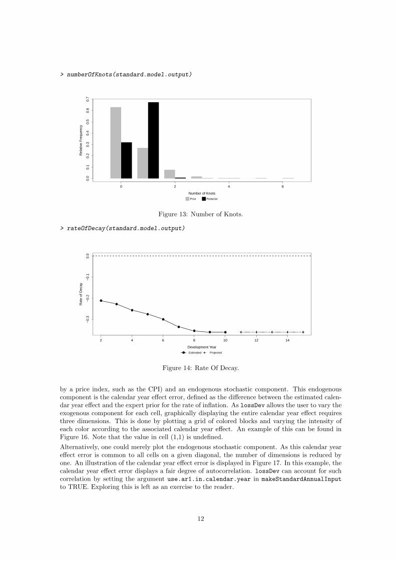
> numberOfKnots(standard.model.output)

0 2 4 6

0.0

0.1

0.2

0.3

0.4

0.5

0.6

0.7

Number of Knots

Rel

ativ

e F

requ

ency

Prior Posterior

Figure 13: Number of Knots.

> rateOfDecay(standard.model.output)

2 4 6 8 10 12 14

−0.

3−

0.2

−0.

10.

0

Development Year

Rat

e of

Dec

ay

●

●

●

●

●

●

●● ●

● Estimated Projected

Figure 14: Rate Of Decay.

by a price index, such as the CPI) and an endogenous stochastic component. This endogenouscomponent is the calendar year effect error, defined as the difference between the estimated calen-dar year effect and the expert prior for the rate of inflation. As lossDev allows the user to vary theexogenous component for each cell, graphically displaying the entire calendar year effect requiresthree dimensions. This is done by plotting a grid of colored blocks and varying the intensity ofeach color according to the associated calendar year effect. An example of this can be found inFigure 16. Note that the value in cell (1,1) is undefined.

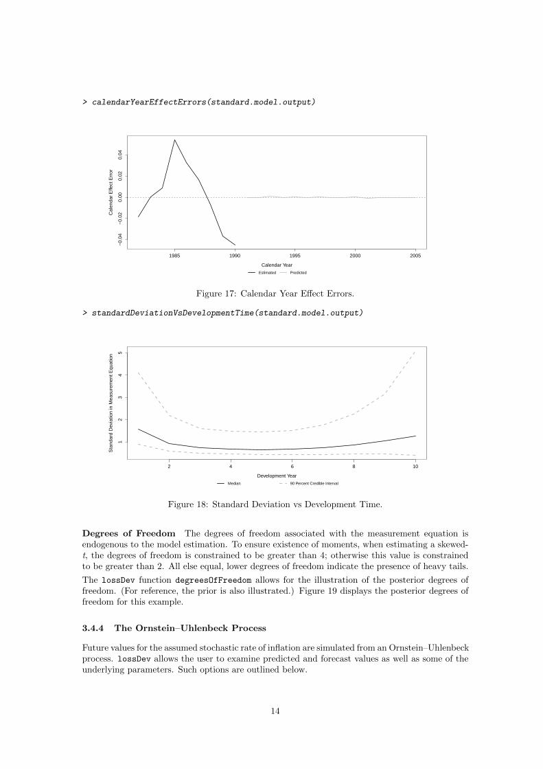
Alternatively, one could merely plot the endogenous stochastic component. As this calendar yeareffect error is common to all cells on a given diagonal, the number of dimensions is reduced byone. An illustration of the calendar year effect error is displayed in Figure 17. In this example, thecalendar year effect error displays a fair degree of autocorrelation. lossDev can account for suchcorrelation by setting the argument use.ar1.in.calendar.year in makeStandardAnnualInput

to TRUE. Exploring this is left as an exercise to the reader.

12

> exposureGrowth(standard.model.output)

1982 1984 1986 1988 1990

−0.

08−

0.06

−0.

04−

0.02

0.00

Accident Year

Rat

e of

Exp

osur

e G

row

th (

Net

of C

alen

dar

Year

Effe

ct)

●

●

●

●

●

●

●

●

●

●

● ●Rate of Exposure Growth Future Rate of Growth Stationary Mean

Figure 15: Exposure Growth.

> calendarYearEffect(standard.model.output)

Development Year

Acc

iden

t Yea

r

1982

1984

1986

1988

1990

5 10 15

0.00

0.02

0.04

0.06

0.08

Figure 16: Calendar Year Effect.

Changes In Variance As development time progresses, the number of transactions that com-prise a given incremental payment declines. This can lead to an increase in the variance of thelog incremental payments even as the level of the payments may decrease. In order to accountfor this potential increase in variance, the model (optionally) allows for the scale parameter of theStudent-t to vary with development time. This scale parameter is smoothed via a second-orderrandom walk on the log scale. As a result, the standard deviation can vary for each developmentyear. An example is displayed in Figure 18.

Skewness Parameter The measurement equation for the log incremental payments is (option-ally) a skewed-t. skewnessParameter allows for the illustration of the posterior skewness param-eter. (For reference, the prior is also illustrated.) While the skewness parameter does not directlytranslate into the estimated skewness, the two are related. For instance, a skewness parameter ofzero would correspond to zero skew. An example is displayed in Figure 19.

13

> calendarYearEffectErrors(standard.model.output)

1985 1990 1995 2000 2005

−0.

04−

0.02

0.00

0.02

0.04

Calendar Year

Cal

enda

r E

ffect

Err

or

Estimated Predicted

Figure 17: Calendar Year Effect Errors.

> standardDeviationVsDevelopmentTime(standard.model.output)

2 4 6 8 10

12

34

5

Development Year

Sta

ndar

d D

evia

tion

in M

easu

rem

ent E

quat

ion

Median 90 Percent Credible Interval

Figure 18: Standard Deviation vs Development Time.

Degrees of Freedom The degrees of freedom associated with the measurement equation isendogenous to the model estimation. To ensure existence of moments, when estimating a skewed-t, the degrees of freedom is constrained to be greater than 4; otherwise this value is constrainedto be greater than 2. All else equal, lower degrees of freedom indicate the presence of heavy tails.

The lossDev function degreesOfFreedom allows for the illustration of the posterior degrees offreedom. (For reference, the prior is also illustrated.) Figure 19 displays the posterior degrees offreedom for this example.

3.4.4 The Ornstein–Uhlenbeck Process

Future values for the assumed stochastic rate of inflation are simulated from an Ornstein–Uhlenbeckprocess. lossDev allows the user to examine predicted and forecast values as well as some of theunderlying parameters. Such options are outlined below.

14

> skewnessParameter(standard.model.output)

−8 −6 −4 −2 0

0.00

0.15

0.30

Skewness Parameter

Den

sity

Prior Posterior

0 500 1000 1500 2000 2500 3000

−10

−6

−2

Sample

Ske

wne

ss P

aram

eter

Figure 19: Skewness Parameter.

> degreesOfFreedom(standard.model.output)

5 10 15

0.00

0.10

Degrees of Freedom

Den

sity

Prior Posterior

0 500 1000 1500 2000 2500 3000

515

25

Sample

Deg

rees

of F

reed

om

Figure 20: Degrees Of Freedom.

Fit and Forecast To display the fitted values vs the observed values (as well as the forecast val-ues) the user must use the function stochasticInflation. The chart for the example illustratedabove is displayed in Figure 21.

Stationary Mean The Ornstein–Uhlenbeck process has a stationary mean; disturbances fromthis mean are assumed to be correlated. Specifically, the projected rate of inflation will (geomet-rically) approach the stationay mean as time progresses. This stationary mean can be graphedwith the function StochasticInflationStationaryMean. The chart for the example illustratedabove is displayed in Figure 22.

Autocorrelation The Ornstein – Uhlenbeck process assumes that the influence of a disturbancedecays geometrically with time. The parameter governing this rate is traditionally referred to asρ. To obtain this value, call the function StochasticInflationRhoParameter. The chart for theexample illustrated above is displayed in Figure 23.

15

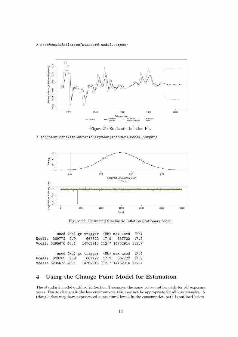
> stochasticInflation(standard.model.output)

1920 1940 1960 1980 2000

−0.

10−

0.05

0.00

0.05

0.10

0.15

Calendar Year

Rat

e of

Infla

tion

(Act

ual a

nd P

redi

cted

)

ActualPredicted/Forecast

90 PercentCredible Interval

StationaryMean

Figure 21: Stochastic Inflation Fit.

> stochasticInflationStationaryMean(standard.model.output)

0.00 0.02 0.04 0.06

010

2030

(Log) Inflation Stationary Mean

Den

sity

Posterior

0 500 1000 1500 2000 2500 3000

−0.

5−

0.2

0.1

Sample

(Log

) In

flatio

n S

tatio

nary

Mea

n

Figure 22: Estimated Stochastic Inflation Stationary Mean.

used (Mb) gc trigger (Mb) max used (Mb)

Ncells 369772 9.9 667722 17.9 667722 17.9

Vcells 6295676 48.1 14762915 112.7 14762914 112.7

used (Mb) gc trigger (Mb) max used (Mb)

Ncells 369765 9.9 667722 17.9 667722 17.9

Vcells 6295673 48.1 14762915 112.7 14762914 112.7

4 Using the Change Point Model for Estimation

The standard model outlined in Section 3 assumes the same consumption path for all exposureyears. Due to changes in the loss environment, this may not be appropriate for all loss triangles. Atriangle that may have experienced a structural break in the consumption path is outlined below.

16

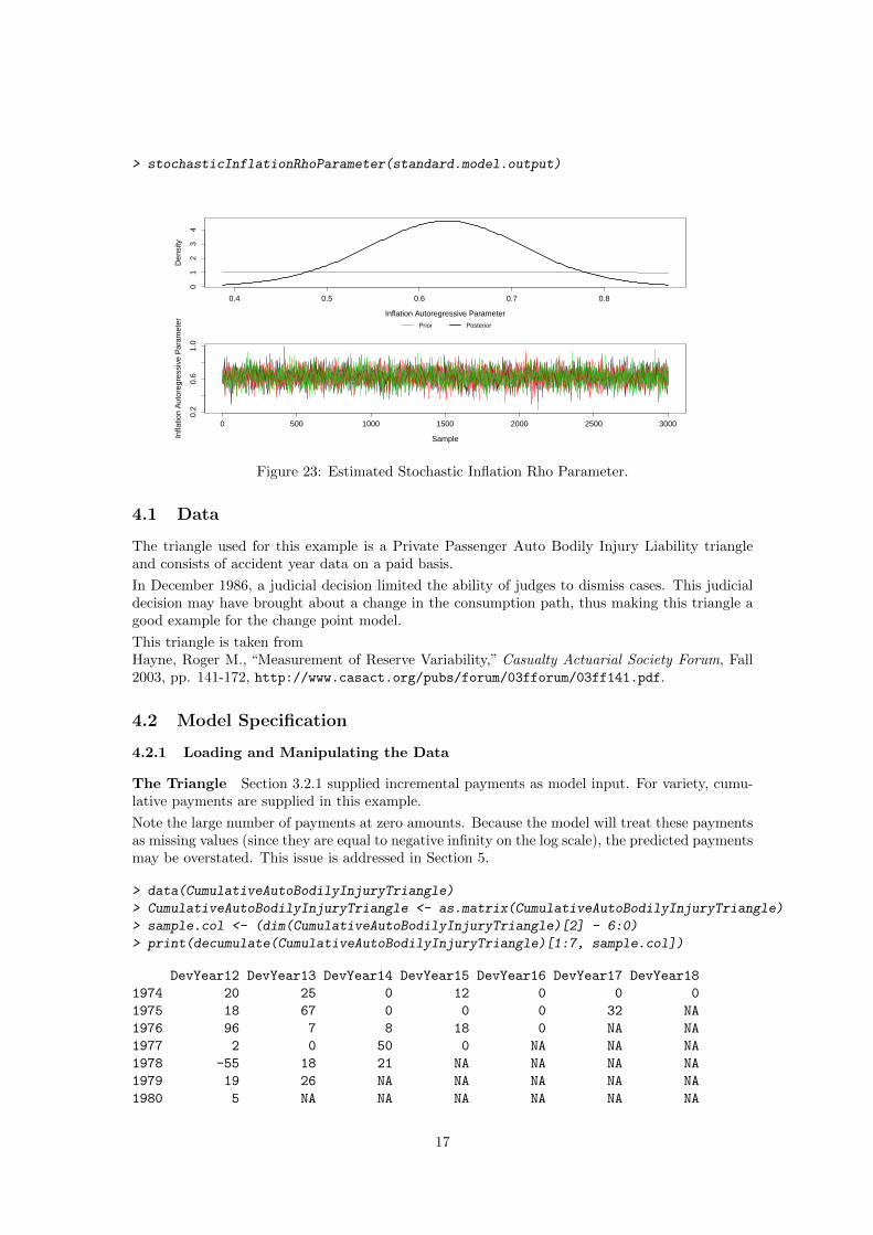
> stochasticInflationRhoParameter(standard.model.output)

0.4 0.5 0.6 0.7 0.8

01

23

4

Inflation Autoregressive Parameter

Den

sity

Prior Posterior

0 500 1000 1500 2000 2500 3000

0.2

0.6

1.0

SampleInfla

tion

Aut

oreg

ress

ive

Par

amet

er

Figure 23: Estimated Stochastic Inflation Rho Parameter.

4.1 Data

The triangle used for this example is a Private Passenger Auto Bodily Injury Liability triangleand consists of accident year data on a paid basis.

In December 1986, a judicial decision limited the ability of judges to dismiss cases. This judicialdecision may have brought about a change in the consumption path, thus making this triangle agood example for the change point model.

This triangle is taken fromHayne, Roger M., “Measurement of Reserve Variability,” Casualty Actuarial Society Forum, Fall2003, pp. 141-172, http://www.casact.org/pubs/forum/03fforum/03ff141.pdf.

4.2 Model Specification

4.2.1 Loading and Manipulating the Data

The Triangle Section 3.2.1 supplied incremental payments as model input. For variety, cumu-lative payments are supplied in this example.

Note the large number of payments at zero amounts. Because the model will treat these paymentsas missing values (since they are equal to negative infinity on the log scale), the predicted paymentsmay be overstated. This issue is addressed in Section 5.

> data(CumulativeAutoBodilyInjuryTriangle)

> CumulativeAutoBodilyInjuryTriangle <- as.matrix(CumulativeAutoBodilyInjuryTriangle)

> sample.col <- (dim(CumulativeAutoBodilyInjuryTriangle)[2] - 6:0)

> print(decumulate(CumulativeAutoBodilyInjuryTriangle)[1:7, sample.col])

DevYear12 DevYear13 DevYear14 DevYear15 DevYear16 DevYear17 DevYear18

1974 20 25 0 12 0 0 0

1975 18 67 0 0 0 32 NA

1976 96 7 8 18 0 NA NA

1977 2 0 50 0 NA NA NA

1978 -55 18 21 NA NA NA NA

1979 19 26 NA NA NA NA NA

1980 5 NA NA NA NA NA NA

17


The Stochastic Inflation Expert Prior The MCPI (Medical Care Component of the CPI) ischosen as a an expert prior for the stochastic rate of inflation. While in Section 3.2.1 the expertprior did not extend beyond the observed diagonals (for realism), here a few extra observed yearsof the MCPI inflation are used for illustration purposes.

> data(MCPI)

> MCPI <- as.matrix(MCPI)[, 1]

> MCPI.rate <- MCPI[-1]/MCPI[-length(MCPI)] - 1

> print(MCPI.rate[(-10):0 + length(MCPI.rate)])

1997 1998 1999 2000 2001 2002 2003

0.02804557 0.03196931 0.03510946 0.04070231 0.04601227 0.04692082 0.04026611

2004 2005 2006 2007

0.04375631 0.04224444 0.04022277 0.04418203

> MCPI.years <- as.integer(names(MCPI.rate))

> max.exp.year <- max(as.integer(dimnames(CumulativeAutoBodilyInjuryTriangle)[[1]]))

> years.to.keep <- MCPI.years <= max.exp.year + 3

> MCPI.rate <- MCPI.rate[years.to.keep]

4.2.2 Selection of Model Options

While makeStandardAnnualInput (Section 3.2.2) is used to specify models without a change point(i.e., structural break), makeBreakAnnualInput is used to specify models with a change point.makeBreakAnnualInput has most of its arguments in common with makeStandardAnnualInput,and all these common arguments carry their meanings forward. However, makeBreakAnnualInputadds a few new arguments; these are for specifying the location of the structural break.

Most notable is the argument first.year.in.new.regime which, as the name suggests, indicatesthe first year in which the new consumption path applies. This argument can be supplied witha single value, in which case the model will give a hundred percent probability that this year isthe first year in the new regime. However, this argument can also be supplied with a range ofcontiguous years, and the model will then estimate the first year in the new regime. Because thepossible break occurs in late 1986, the range of years chosen for this example is 1986 to 1987.

The prior for the first year in the new regime is a discretized beta distribution. The user has the op-tion of choosing the parameters for this prior by setting the argument prior.for.first.year.in.new.regime.Here, since the change was in late 1986, we choose a prior that accords more probability to thelater year.

The argument bound.for.skewness.parameter is set to 5. This avoids the MCMC chain from“getting stuck” in the lower tail of the distribution (in this particular example). One should usethe function skewnessParemeter (Figure 37) to evaluate the need to set this value. If the useris experiencing difficulties with the skewed-t, he may wish to use the non-skewed-t by setting theargument use.skew.t equal to FALSE (which is the default).

> break.model.input <- makeBreakAnnualInput(cumulative.payments = CumulativeAutoBodilyInjuryTriangle,


+ stoch.inflation.rate = MCPI.rate, first.year.in.new.regime = c(1986,

+ 1987), prior.for.first.year.in.new.regime = c(2, 1),

+ exp.year.type = "ay", extra.dev.years = 5, use.skew.t = TRUE,

+ bound.for.skewness.parameter = 5)

4.3 Estimating the Model

Just like in Section 3.3, the S4 object returned by makeBreakAnnualInput must be supplied tothe function runLossDevModel in order to produce estimates.

18

> break.model.output <- runLossDevModel(break.model.input, burnIn = 30000,

+ sampleSize = 30000, thin = 10)



Allocating nodes

Initializing




Allocating nodes

Graph Size: 19945

[1] "Update took 1.280564 hours"

4.4 Examining Output

4.4.1 Assessing Convergence

As discussed, the user must examine the MCMC runs for convergence using the same functionsmentioned in Section 3.4.1. To avoid repetition, only a few of the previously illustrated charts willbe discussed below.

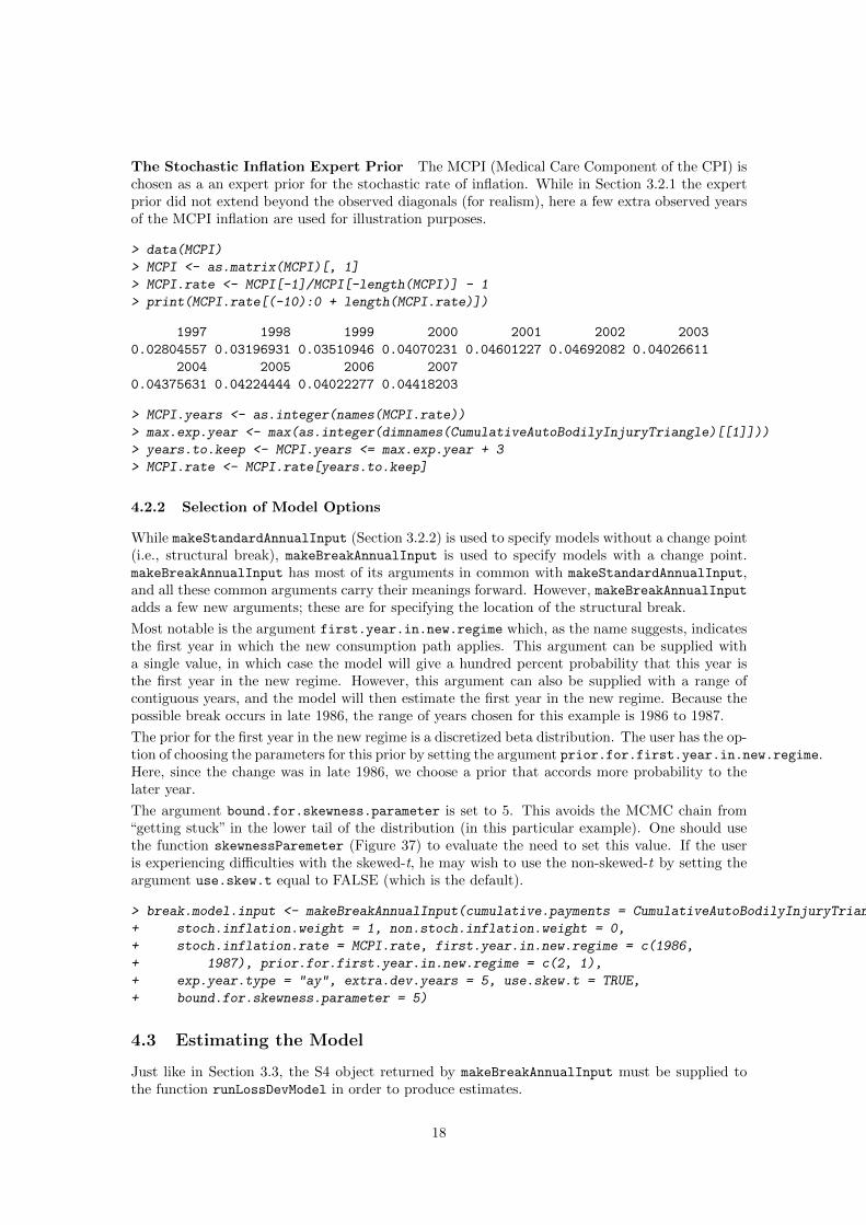
Because the change point model has two consumption paths, the method consumptionPathTra-

cePlot for output related to this model has an additional argument when it comes to specifing theconsumption path. If the argument preBreak equals TRUE, then the trace for the consumptionpath relevant to exposure years prior to the structural break will be plotted. Otherwise, the tracefor the consumption path relevant to exposure years after the break will be plotted.

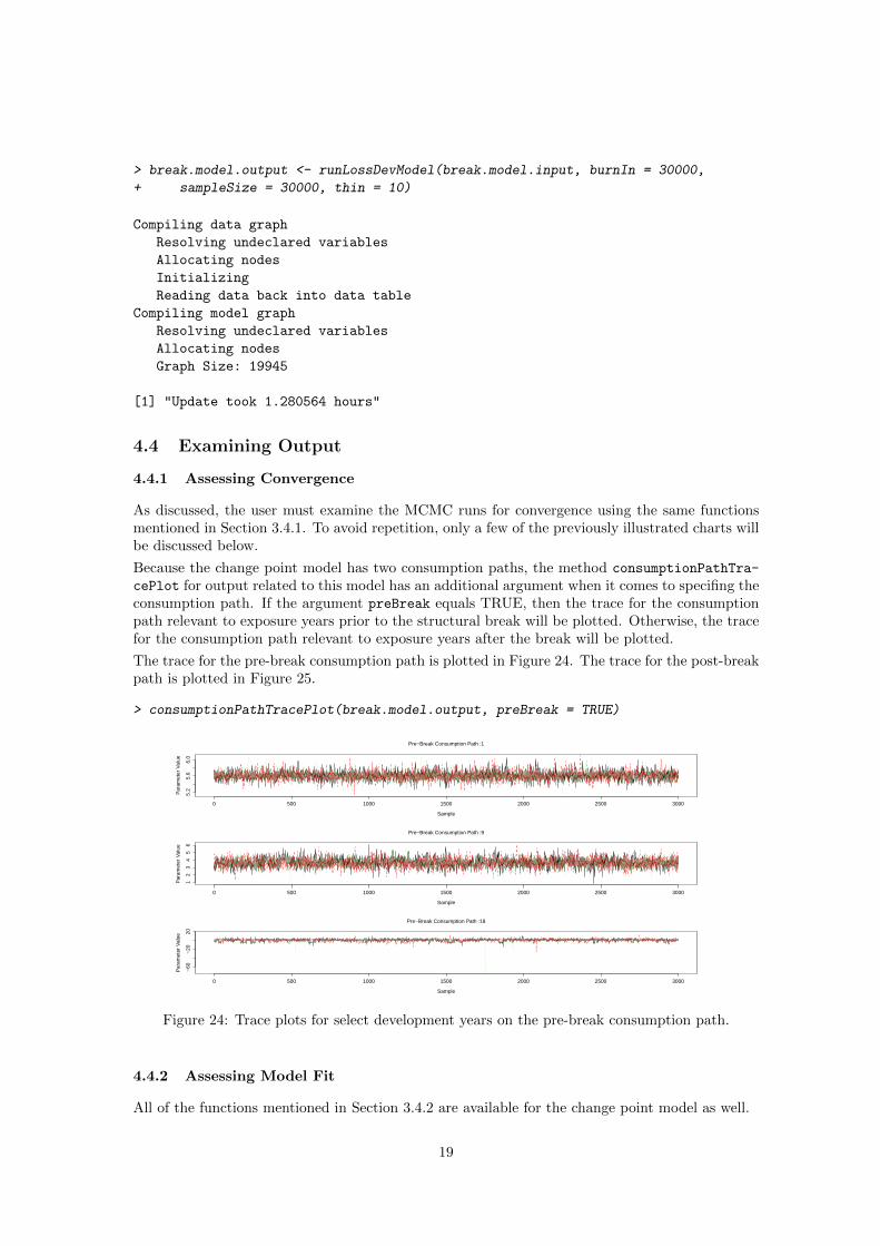
The trace for the pre-break consumption path is plotted in Figure 24. The trace for the post-breakpath is plotted in Figure 25.

> consumptionPathTracePlot(break.model.output, preBreak = TRUE)

0 500 1000 1500 2000 2500 3000

5.2

5.6

6.0

Pre−Break Consumption Path :1

Sample

Par

amet

er V

alue

0 500 1000 1500 2000 2500 3000

12

34

56


Sample

Par

amet

er V

alue

0 500 1000 1500 2000 2500 3000

−60

−20

20


Sample

Par

amet

er V

alue

Figure 24: Trace plots for select development years on the pre-break consumption path.

4.4.2 Assessing Model Fit

All of the functions mentioned in Section 3.4.2 are available for the change point model as well.

19

> consumptionPathTracePlot(break.model.output, preBreak = FALSE)

0 500 1000 1500 2000 2500 3000

4.5

5.5

Post−Break Consumption Path :1

Sample

Par

amet

er V

alue

0 500 1000 1500 2000 2500 3000

13

5


Sample

Par

amet

er V

alue

0 500 1000 1500 2000 2500 3000

−60

−20

20


Sample

Par

amet

er V

alue

Figure 25: Trace plots for select development years on the post-break consumption path.

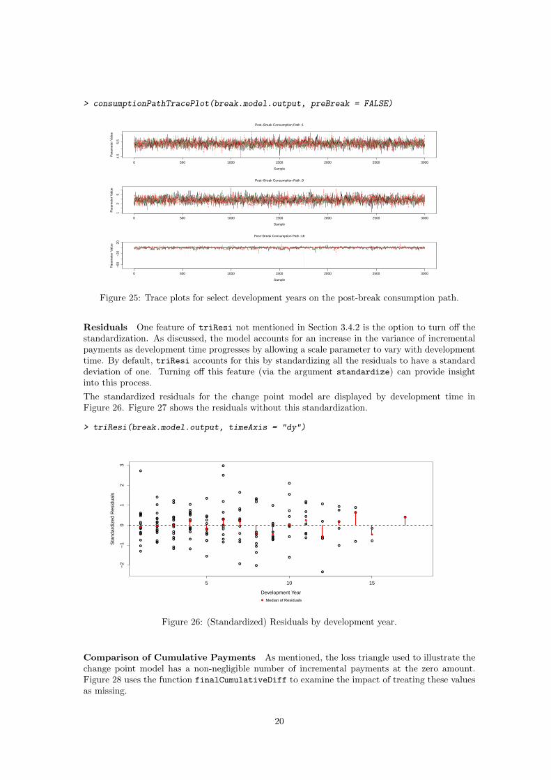
Residuals One feature of triResi not mentioned in Section 3.4.2 is the option to turn off thestandardization. As discussed, the model accounts for an increase in the variance of incrementalpayments as development time progresses by allowing a scale parameter to vary with developmenttime. By default, triResi accounts for this by standardizing all the residuals to have a standarddeviation of one. Turning off this feature (via the argument standardize) can provide insightinto this process.

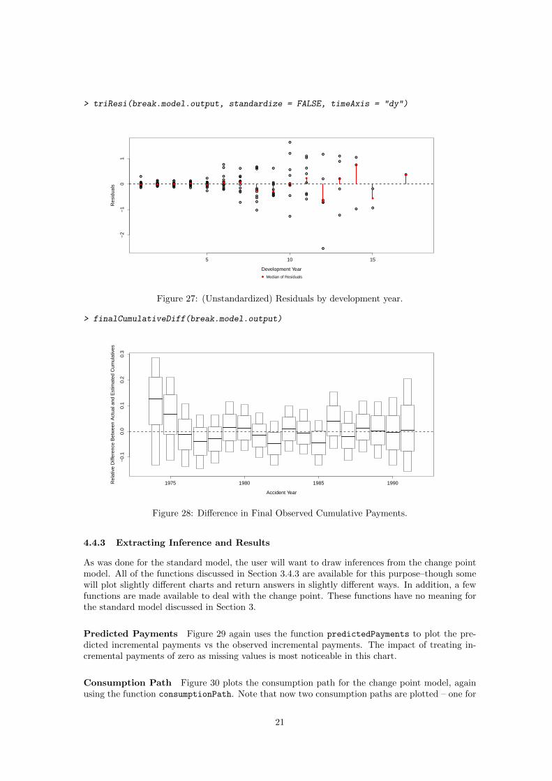
The standardized residuals for the change point model are displayed by development time inFigure 26. Figure 27 shows the residuals without this standardization.

> triResi(break.model.output, timeAxis = "dy")

5 10 15

−2

−1

01

23

Development Year

Sta

ndar

dize

d R

esid

uals

●●

●

●

●

●

●

●●●●

●

●

●

●

●

●

● ●

●

●

●

●

●●

●

●

●

●

●

●

●

●

●

●

●

●

●

●

●

●

●

●

●

●●

●

●

●●

●●

●

●

●

●

●

●●

●

●

●

●

●

●

●●

●

●

●

●

●

●

●

●

●

●

●

●

●

●

●

●

●

●

●

●

●

●

●

●

●

●

●

●●

●

●

●

●●

●

●

●

●

●

●

●

●

●●

●

●

●

●

●

●

●●●

●

●

●

●

●

●●

●

●●

●

●

●

●

●

●

●

●

●

●

●

●

● ●●

●

●

●

●

●

●

●

●

●

●

●

●

●

●

●

●●

●

●

●

●●

● ●

●

●

●

●

●

●

●


Figure 26: (Standardized) Residuals by development year.

Comparison of Cumulative Payments As mentioned, the loss triangle used to illustrate thechange point model has a non-negligible number of incremental payments at the zero amount.Figure 28 uses the function finalCumulativeDiff to examine the impact of treating these valuesas missing.

20

> triResi(break.model.output, standardize = FALSE, timeAxis = "dy")

5 10 15

−2

−1

01

Development Year

Res

idua

ls ●●●

●

●●

●●●●●●●●●●

●● ●

●

●●●●●●●

●●●●●●●● ●

●

●●●

●●

●●

●●●

●

●●● ●●

●●●●●●●●●

●

●●●

●

●

●

●●●

●●

●

●●

●●●

●

●

●

●●

●

●

●●

●

●●

●

●

●●

●●

●

●●

●

●

●

●

●

●

●

●

●●

●●

●

●

●

●

●●●

●

●

●

●

●

● ●

●

●●

●

●

●

●

●

●

●

●

●

●

●

●

●

●●

●

●

●

●

●

●

●

●

●

●

●

●

●

●

●

● ● ● ●●

● ●

●●

●

●

●

●

●

●

●


Figure 27: (Unstandardized) Residuals by development year.

> finalCumulativeDiff(break.model.output)

1975 1980 1985 1990

−0.

10.

00.

10.

20.

3

Accident Year

Rel

ativ

e D

iffer

ence

Bet

wee

n A

ctua

l and

Est

imat

ed C

umul

ativ

es

Figure 28: Difference in Final Observed Cumulative Payments.

4.4.3 Extracting Inference and Results

As was done for the standard model, the user will want to draw inferences from the change pointmodel. All of the functions discussed in Section 3.4.3 are available for this purpose–though somewill plot slightly different charts and return answers in slightly different ways. In addition, a fewfunctions are made available to deal with the change point. These functions have no meaning forthe standard model discussed in Section 3.

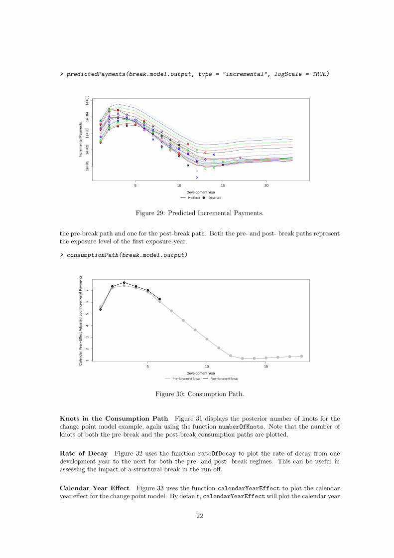
Predicted Payments Figure 29 again uses the function predictedPayments to plot the pre-dicted incremental payments vs the observed incremental payments. The impact of treating in-cremental payments of zero as missing values is most noticeable in this chart.

Consumption Path Figure 30 plots the consumption path for the change point model, againusing the function consumptionPath. Note that now two consumption paths are plotted – one for

21

> predictedPayments(break.model.output, type = "incremental", logScale = TRUE)

5 10 15 20

1e+

011e

+02

1e+

031e

+04

1e+

05

Development Year

Incr

emen

tal P

aym

ents

●

●

● ●●

●

●

●

●

●

●

●●

●

●

●●

●

● ●

●

●

●

●

●

●

●

●

●

●

●● ●

●

●

●

●

●

● ●

●●

●

●

●

●● ●

●

●●

●

●

●

●

●

●

●

●●

●

●

●

● ●●

●

●●

●

●

●

●

●

●

●

●

●●

●

●

●

●

●

● ●

●

●

●

●

●

●

●

●

●

● ● ●

●

●

●●

●

●

●

●

● ●●

●

●

●

●

●

●

●

●●

●

●

●

●

●●

●

● ●●

●

●

●

●

●

●●

●

●

●

●

●

●●

●

●

●

●

●●

●

●

●

●●

●

●

●●

●

●

●


Figure 29: Predicted Incremental Payments.

the pre-break path and one for the post-break path. Both the pre- and post- break paths representthe exposure level of the first exposure year.

> consumptionPath(break.model.output)

5 10 15

12

34

56

7

Development Year

Cal

enda

r Ye

ar−

Effe

ct A

djus

ted

Log

Incr

emen

al P

aym

ents

●

●

●

●

●

●

●

●

●

●

●

●

● ● ● ● ● ●

●

●

●

●

●

●

Pre−Structrural Break Post−Structural Break

Figure 30: Consumption Path.

Knots in the Consumption Path Figure 31 displays the posterior number of knots for thechange point model example, again using the function numberOfKnots. Note that the number ofknots of both the pre-break and the post-break consumption paths are plotted.

Rate of Decay Figure 32 uses the function rateOfDecay to plot the rate of decay from onedevelopment year to the next for both the pre- and post- break regimes. This can be useful inassessing the impact of a structural break in the run-off.

Calendar Year Effect Figure 33 uses the function calendarYearEffect to plot the calendaryear effect for the change point model. By default, calendarYearEffect will plot the calendar year

22

> numberOfKnots(break.model.output)

0 2 4 6 8 10

0.0

0.1

0.2

0.3

0.4

0.5

0.6

Pre−Structural Break

Number of Knots

Rel

ativ

e F

requ

ency

Prior Posterior

0 1 2 3 4

0.0

0.1

0.2

0.3

0.4

0.5

0.6

Post−Structural Break

Number of Knots

Rel

ativ

e F

requ

ency

Figure 31: Number of Knots.

> rateOfDecay(break.model.output)

5 10 15 20

01

23

45

6

Development Year

Rat

e of

Dec

ay

●

●

●

●

● ● ● ● ● ● ●

●

● ● ● ● ●

●

●

● ●

● ● ● ● ● ● ●

●● ● ● ● ● ● ● ● ● ●● ● ● ● ●● ● ● ● ●● ● ● ● ●● ● ● ● ●● ● ● ● ●● ● ● ● ●● ● ● ● ●● ● ● ● ●● ● ● ● ●● ● ● ● ●● ● ● ● ●● ● ● ● ●● ● ● ● ●● ● ● ● ●● ● ● ● ●● ● ● ● ●● ● ● ● ●● ● ● ● ●

● ● ●Pre−StructruralBreak

Post−StructuralBreak

Pre/Post−StructruralBreak

Figure 32: Rate Of Decay.

effect for all (observed and projected) incremental payments. Setting the argument restricted-Size to TRUE will plot the calendar year effect for only the observed incremental payments andthe projected incremental payments needed to “square” the triangle. This feature can be usefulfor insurance lines with long tails.

Figure 34 shows the calendar year effect error which is plotted using the function calendarYear-

EffectErrors.

Autocorrelation in Calendar Year Effect The autocorrelation exhibited in Figure 34 is toostrong to ignore. Figure 35 illustrates the use of makeBreakAnnualInput’s argument use.ar1.in.calendar.year.

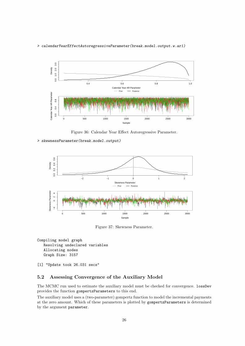
Setting use.ar1.in.calendar.year to TRUE enables the use of an additional function: cal-

endarYearEffectAutoregressiveParameter. This function will plot the autoregressive parame-ter associated with the calendar year effect error. Figure 36 illustrates the use of this function.

23

> calendarYearEffect(break.model.output)

Development Year

Acc

iden

t Yea

r

1975

1980

1985

1990

5 10 15 20

−0.2

0.0

0.2

0.4

0.6

Figure 33: Calendar Year Effect.

> calendarYearEffectErrors(break.model.output)

1975 1980 1985 1990 1995 2000 2005

−0.

4−

0.2

0.0

0.2

0.4

Calendar Year

Cal

enda

r E

ffect

Err

or

Estimated Predicted

Figure 34: Calendar Year Effect Errors (Without AR1).

Skewness Parameter Figure 37 displays the skewness parameter for the change point model ex-ample by using the function skewnessParemeter. The result of setting bound.for.skewness.parameter

to 5 is visible in the chart.

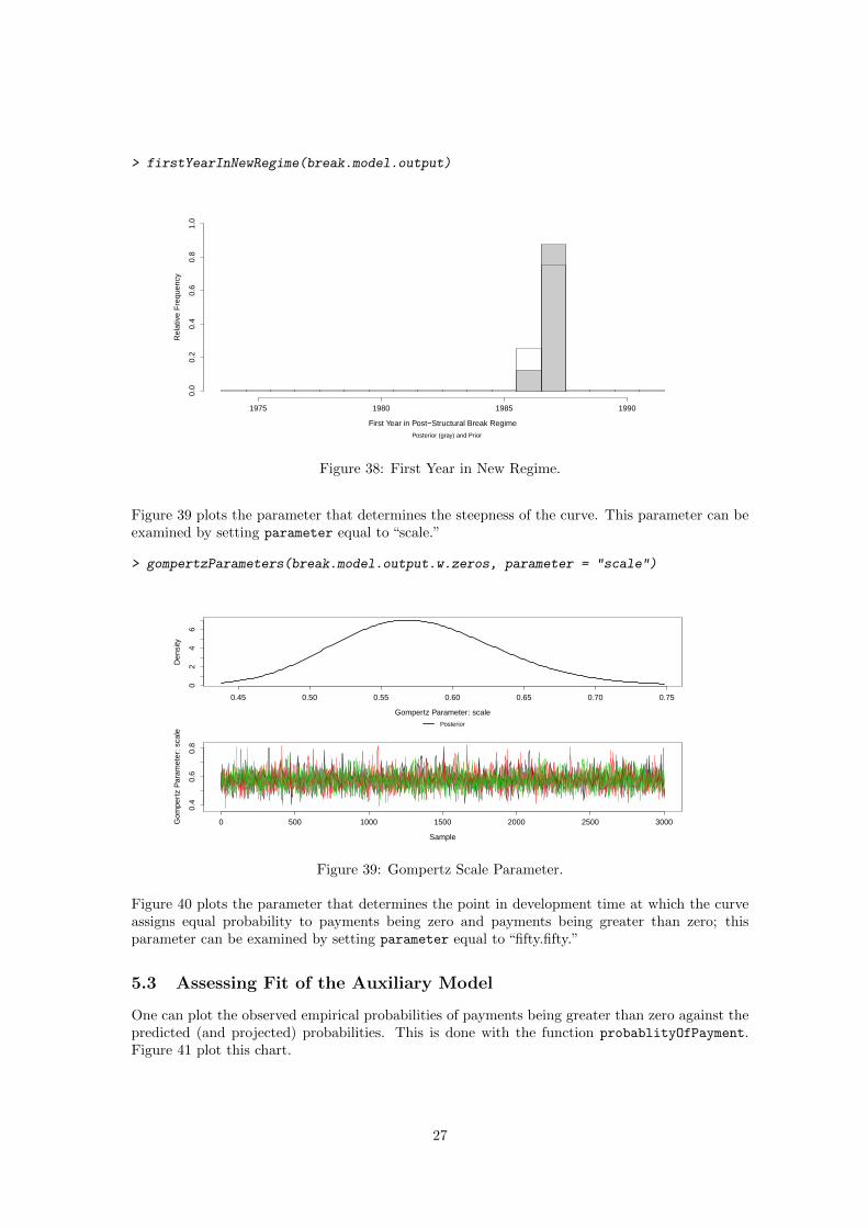
First Year in New Regime The posterior for the first year in which the post-break consump-tion path applies can be obtained via the function firstYearInNewRegime. Figure 38 shows theposterior (and prior) for the first year in the new regime. Note how the choice of the argumentprior.for.first.year.in.new.regime to makeBreakAnnualInput has affected the prior.

5 Accounting for Incremental Payments of Zero

As mentioned in Section 4.2.1 and illustrated in Figure 29, the triangle used as an example for thechange point model contains several incremental payments of zero which, if ignored, could cause

24

> break.model.input.w.ar1 <- makeBreakAnnualInput(cumulative.payments = CumulativeAutoBodilyInjuryTriangle,


+ stoch.inflation.rate = MCPI.rate, first.year.in.new.regime = c(1986,

+ 1987), prior.for.first.year.in.new.regime = c(2, 1),

+ exp.year.type = "ay", extra.dev.years = 5, use.skew.t = TRUE,

+ bound.for.skewness.parameter = 5, use.ar1.in.calendar.year = TRUE)

> break.model.output.w.ar1 <- runLossDevModel(break.model.input.w.ar1,

+ burnIn = 30000, sampleSize = 30000, thin = 10)



Allocating nodes

Initializing




Allocating nodes

Graph Size: 26907

[1] "Update took 1.313121 hours"

> calendarYearEffectErrors(break.model.output.w.ar1)

1975 1980 1985 1990 1995 2000 2005

−0.

20.

00.

20.

4

Calendar Year

Cal

enda

r E

ffect

Err

or

Estimated Predicted

Figure 35: Calendar Year Effect Errors (With AR1).

the predicted losses to be overestimated.

lossDev provides a means to account for these payments at the zero amount. This is done byestimating a secondary, auxiliary model to determine the probably that a payment will be greaterthan zero. Predicted payments are then weighted by this probability.

5.1 Estimating the Auxiliary Model

To account for payments at zero amounts, the function accountForZeroPayments is called with thefirst argument being an object returned from a call to runLossDevModel. This function will thenreturn another object which, when called by certain functions already mentioned, will incorporateinto the calculation the probability that any particular payment is zero.

> break.model.output.w.zeros <- accountForZeroPayments(break.model.output)

25

> calendarYearEffectAutoregressiveParameter(break.model.output.w.ar1)

0.4 0.6 0.8 1.0

0.0

1.0

2.0

3.0

Calendar Year AR Parameter

Den

sity

Prior Posterior

0 500 1000 1500 2000 2500 3000

0.0

0.4

0.8

Sample

Cal

enda

r Ye

ar A

R P

aram

eter

Figure 36: Calendar Year Effect Autoregressive Parameter.

> skewnessParameter(break.model.output)

−2 −1 0 1 2

0.0

0.2

0.4

0.6

Skewness Parameter

Den

sity

Prior Posterior

0 500 1000 1500 2000 2500 3000

−4

02

4

Sample

Ske

wne

ss P

aram

eter

Figure 37: Skewness Parameter.



Allocating nodes

Graph Size: 3157

[1] "Update took 26.031 secs"

5.2 Assessing Convergence of the Auxiliary Model

The MCMC run used to estimate the auxiliary model must be checked for convergence. lossDevprovides the function gompertzParameters to this end.

The auxiliary model uses a (two-parameter) gompertz function to model the incremental paymentsat the zero amount. Which of these parameters is plotted by gompertzParameters is determinedby the argument parameter.

26

> firstYearInNewRegime(break.model.output)

First Year in Post−Structural Break Regime

Rel

ativ

e F

requ

ency

1975 1980 1985 1990

0.0

0.2

0.4

0.6

0.8

1.0

Posterior (gray) and Prior

Figure 38: First Year in New Regime.

Figure 39 plots the parameter that determines the steepness of the curve. This parameter can beexamined by setting parameter equal to “scale.”

> gompertzParameters(break.model.output.w.zeros, parameter = "scale")

0.45 0.50 0.55 0.60 0.65 0.70 0.75

02

46

Gompertz Parameter: scale

Den

sity

Posterior

0 500 1000 1500 2000 2500 3000

0.4

0.6

0.8

Sample

Gom

pert

z P

aram

eter

: sca

le

Figure 39: Gompertz Scale Parameter.

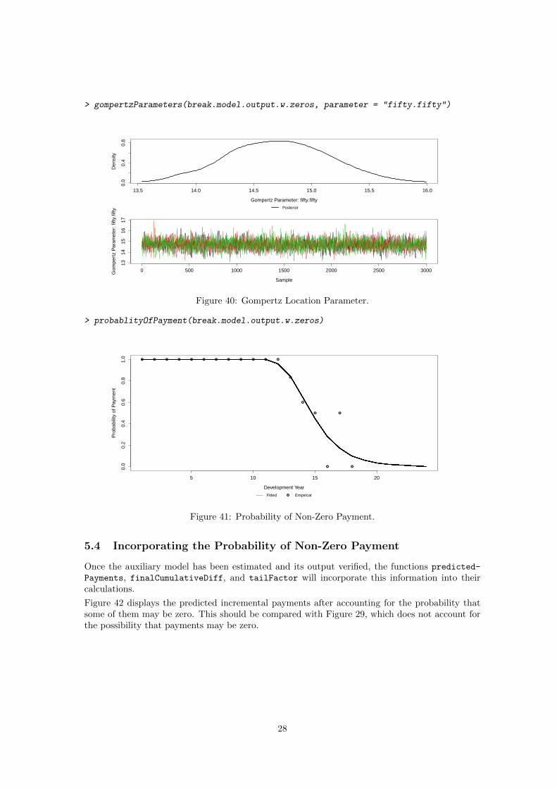
Figure 40 plots the parameter that determines the point in development time at which the curveassigns equal probability to payments being zero and payments being greater than zero; thisparameter can be examined by setting parameter equal to “fifty.fifty.”

5.3 Assessing Fit of the Auxiliary Model

One can plot the observed empirical probabilities of payments being greater than zero against thepredicted (and projected) probabilities. This is done with the function probablityOfPayment.Figure 41 plot this chart.

27

> gompertzParameters(break.model.output.w.zeros, parameter = "fifty.fifty")

13.5 14.0 14.5 15.0 15.5 16.0

0.0

0.4

0.8

Gompertz Parameter: fifty.fifty

Den

sity

Posterior

0 500 1000 1500 2000 2500 3000

1314

1516

17

Sample

Gom

pert

z P

aram

eter

: fift

y.fif

ty

Figure 40: Gompertz Location Parameter.

> probablityOfPayment(break.model.output.w.zeros)

5 10 15 20

0.0

0.2

0.4

0.6

0.8

1.0

Development Year

Pro

babi

lity

of P

aym

ent

● ● ● ● ● ● ● ● ● ● ● ●

●

●

●

●

●

●

●Fitted Empirical

Figure 41: Probability of Non-Zero Payment.

5.4 Incorporating the Probability of Non-Zero Payment

Once the auxiliary model has been estimated and its output verified, the functions predicted-

Payments, finalCumulativeDiff, and tailFactor will incorporate this information into theircalculations.

Figure 42 displays the predicted incremental payments after accounting for the probability thatsome of them may be zero. This should be compared with Figure 29, which does not account forthe possibility that payments may be zero.

28

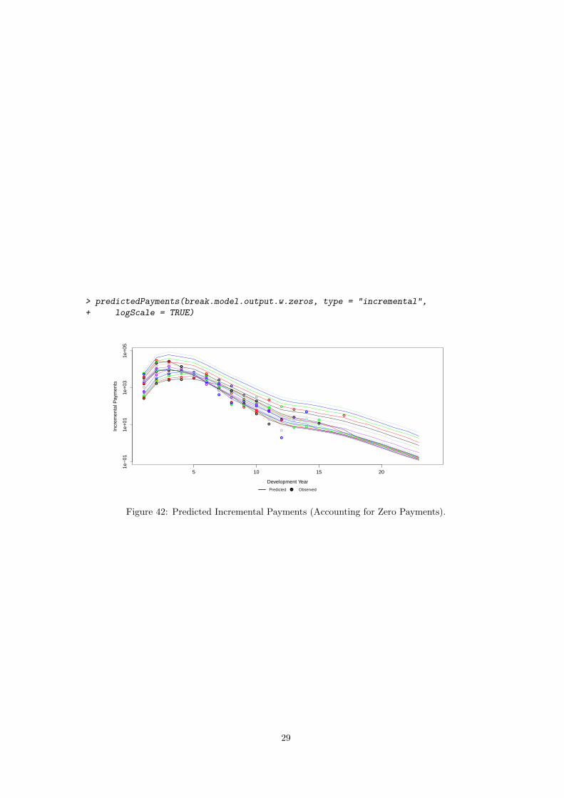
> predictedPayments(break.model.output.w.zeros, type = "incremental",

+ logScale = TRUE)

5 10 15 20

1e−

011e

+01

1e+

031e

+05

Development Year

Incr

emen

tal P

aym

ents

●

●

● ●●

●

●

●

●

●

●

●●

●

●

● ●●

● ●

●

●

●

●

●

●

●

●

●

●

●● ●

●

●

●

●

●

● ●

● ●

●

●

●

●● ●

●

●●

●

●

●

●

●

●

●

●●

●

●

●

● ●●

●

●●

●

●

●●

●●

●

●

●●

●

●●

●

●● ●

●

●

●●

●

●

●

●

●

● ● ●

●

●

●●

●

●

●

●

● ●●

●

●

●

●

●

●

●

●●

●

●

●

●

● ●

●

● ●●

●

●

●

●

●

● ●●

●

●

●

●

●●

●

●

●

●

●●

●

●

●

●●

●

●

●●

●

●

●


Figure 42: Predicted Incremental Payments (Accounting for Zero Payments).

29

robust loss development using mcmc: a...

Documents