International Journal of

Financial Studies

Article

Robust Optimization-Based Commodity PortfolioPerformance

Ramesh Adhikari 1,* , Kyle J. Putnam 2 and Humnath Panta 1

1 School of Business, Humboldt State University, Arcata, CA 95521, USA; humnath.panta@humboldt.edu2 School of Business, Linfield University, McMinnville, OR 97128, USA; kputnam@linfield.edu* Correspondence: ramesh.adhikari@humboldt.edu

Received: 2 August 2020; Accepted: 2 September 2020; Published: 5 September 2020�����������������

Abstract: This paper examines the performance of a naïve equally weighted buy-and-hold portfolioand optimization-based commodity futures portfolios for various lookback and holding periodsusing data from January 1986 to December 2018. The application of Monte Carlo simulation-basedmean-variance and conditional value-at-risk optimization techniques are used to construct the robustcommodity futures portfolios. This paper documents the benefits of applying a sophisticated, robustoptimization technique to construct commodity futures portfolios. We find that a 12-month lookbackperiod contains the most useful information in constructing optimization-based portfolios, and a1-month holding period yields the highest returns among all the holding periods examined inthe paper. We also find that an optimized conditional value-at-risk portfolio using a 12-monthlookback period outperforms an optimized mean-variance portfolio using the same lookback period.Our findings highlight the advantages of using robust optimization for portfolio formation in thepresence of return uncertainty in the commodity futures markets. The results also highlight thepractical importance of choosing the appropriate lookback and holding period when using robustoptimization in the commodity portfolio formation process.

Keywords: commodities; commodity futures; portfolio optimization

JEL Classification: G11; G12; G13

1. Introduction

Optimization-based portfolio construction techniques play a vital role in both pedagogy andpractical applications of finance. Optimization based on mean-variance (MV) and conditionalvalue-at-risk (CVaR) is widely used in the finance literature. The mean-variance approach to portfolioconstruction considers both expected returns and the variance of the returns on risky assets to optimizeportfolio weights and achieve the highest expected return for a given level of risk (Markowitz 1952).Following the seminal work of Markowitz (1952), numerous studies have explored the performance andcharacteristics of optimization-based portfolios: industry value-at-risk (Lwin et al. 2017), mean-varianceefficiency in the presence of background risk (Huang and Yang 2020); asset weighting bounds (Green andHollifield 1992); behavioral mean-variance portfolios (Bi et al. 2018); constrained portfolio estimation(Grauer and Shen 2000); the equally weighted portfolio (DeMiguel et al. 2009); mean-variance portfoliosusing factor models (Fan et al. 2008); various forms of optimization portfolios (Goldfarb and Iyengar2003; Scherer 2007; Tütüncü and Koenig 2004; Zakamulin 2017); conditional value-at-risk (Lim et al.2011); and worst-case optimization (Kim et al. 2013). One of the shortfalls of the standard mean-varianceapproach is that it considers one set of data realization but fails to consider many other possiblerealizations of data that may occur due to various sources of risk.

Int. J. Financial Stud. 2020, 8, 54; doi:10.3390/ijfs8030054 www.mdpi.com/journal/ijfs

Int. J. Financial Stud. 2020, 8, 54 2 of 17

The traditional optimization technique is often an unintentional error maximizer which frequentlyoverweights uncertain statistics. Although it is intuitive and straightforward, the practical applicationof mean-variance analysis is problematic because as the number of assets grows, the weights of theindividual assets do not approach zero as quickly as suggested by naïve notions of diversification(Green and Hollifield 1992). The added benefit of volatility and correlation information is often offsetby the uncertainty with which you measure the statistics. Moreover, mean-variance optimal portfoliosare very sensitive to slight changes in input parameters. The presence of outliers heavily influences theoutcomes of the conventional measure of covariance (Huo et al. 2012). Best and Grauer (1991) show thatin the presence of a budget and non-negativity constraint, the portfolio weights, mean, and variancecan be exceedingly sensitive to changes in individual asset means. For instance, an increase of 11.6%per annum in the mean of any stock in a portfolio can drive nearly half of the constituents away.Such sensitivity via input parameters is very problematic for portfolio optimization because accurateparameter estimation is complicated, particularly for returns (Michaud 1998). Thus, the results fromvarious traditional optimization techniques should be used carefully.

Robust estimation incorporates parameter uncertainty by defining a set of possible values, and theoptimal solution represents the best choice when considering all of the possibilities from the uncertaintyparameters. Aptly, robust estimation is about finding “good objective values” for all iterations ofuncertain input parameters in an optimization problem (Tütüncü and Koenig 2004).1 Additionally,robust optimization-based portfolios are less sensitive to input parameters (Ceria and Stubbs 2006).Robust optimization uses various robust approaches, including improving the robustness of inputs(Jorion 1986), reducing estimation errors using simulation techniques (Michaud and Michaud 2008),and allowing a combination of investor’s views on the model (Black and Litterman 1992). A portfolioconstructed using robust optimization has a higher correlation between the actual expected returnsand the alphas implied from the portfolios (Ceria and Stubbs 2006). Looking at robust measures of riskand return can provide a more reflective and accurate insight into return behavior (Kim and White2004). As a result, robust estimation typically outperforms traditional mean-variance portfolios in avariety of investment scenarios since robust portfolios dampen the uncertainty and sensitivity issuesof standard mean-variance analysis (Kim et al. 2013).

Robust optimization has been used extensively in the field of operations and mathematical opticsto analyze the characteristics of portfolio performance (Calafiore 2007; Elliott and Siu 2010; Goldfarband Iyengar 2003; Natarajan et al. 2009; Shen and Zhang 2008; Zhu and Fukushima 2009). Most ofthe research relating to the computational advantages of robust optimization for investments utilizesbroad market equity and volatility data (Goldfarb and Iyengar 2003; Ceria and Stubbs 2006; Post et al.2019). Tütüncü and Koenig (2004) provide a more in-depth analysis of the equity markets by applyingrobust optimization techniques to large-cap growth, large-cap value, small-cap growth, and small-capvalue and by comparing the behavior of estimates obtained via robust optimization to standardoptimization approaches. They find that portfolios formed using robust optimization tend to havesignificantly improved worst-case behavior and demonstrate stability over long periods. More recently,Kim et al. (2017) conducted a comprehensive empirical analysis of the equity markets to endorse thepractical use of robust optimization by investment managers. They find that robust portfolios areone of the most efficient investment strategies over the long-term (1984–2014) and intermediate-term(five-year sub-periods). Additionally, they note that robust optimization portfolios have lower levelsof risk for similar levels of risk-adjusted returns compared to classical mean-variance portfolios—thatis, the optimized portfolios exhibit a relatively small worst-case loss measure, demonstrating theirsuperiority at allocating risk relative to a set of conservative benchmarks.

1 In practice, there are many different definitions of robustness based on various mathematical formulations. See Kim et al.(2016) for an overview of several optimization methodologies.

Int. J. Financial Stud. 2020, 8, 54 3 of 17

To date, a question that has not been addressed in the literature is whether robust optimizationprovides an advantage in portfolio construction in the commodity futures markets. Similar to the equitymarkets, active management in the commodity futures markets are concerned with the outperformanceof a naïve benchmark portfolio (Gorton and Rouwenhorst 2006; Bhardwaj et al. 2015). Therefore,our objective in this paper is to examine whether robust optimization-based commodity portfoliosoutperform a naïve buy-and-hold commodity futures portfolio. Additionally, we aim to document therisk and return characteristics of such robust commodity portfolios.

There are three-fold contributions of this paper to commodity futures research. First, we addressdata uncertainty by comparing the performance of an equally weighted portfolio against the moresophisticated optimization-based commodity portfolios. Second, we document the most informativelookback period in the robust optimization portfolio formation process. Third, we document theoptimal holding period for the robust optimzation portfolio formation process.

We focus on robust optimization constructed on the traditional mean-variance and conditionalvalue-at-risk measures of risk to create optimally weighted futures portfolios for five diverse commoditysectors—foods and fibers, grains and oilseeds, livestock, energy, and precious metals. The motivationfor investment among commodity sectors, as opposed to individual commodity futures, is due to apreference for diversification among heterogenous assets (Adhikari and Putnam 2020). The simulateddata are generated using a normal distribution with a mean and covariance matrix of prior returnsfrom either a 12-, 15-, or 18-month lookback period. The expected weights are calculated on a rollingbasis by optimizing the objective function, using the simulated data, and rebalancing at the end ofeach holding period (i.e., one month). This process is repeated from January 1986 through December2018. We analyze the performance metrics of three MV robust optimization-based portfolios based onthe three lookback periods—MV12, MV15, and MV18—and three CVaR robust optimization-basedportfolios conditioned on the three lookback periods—CVaR12, CVaR15, and CVaR18. The optimalperforming robust portfolios are subsequently evaluated over 1, 3, 6, 9, and 12-month holding periods.

Our empirical results show that both the MV and CVaR robust optimization-based portfoliosconditioned on return data over the prior 12 months (MV12 and CVaR12, respectively) outperform anaïve buy-and-hold portfolio of commodity futures on a nominal and risk-adjusted basis. We findthat the robust optimization-based portfolios formed using both 15-month and 18-month lookbackperiods fail to outperform an equally weighted commodity futures portfolio. These findings arethought-provoking because they highlight the advantages of robust optimization for dealing withthe uncertainty and sensitivity of the inputs in commodity futures portfolio formation. However,they also suggest a lack of efficacy when return data beyond 12 months is incorporated into theoptimization process.

Since the annual lookback period produces the most desirable results of all the portfolios,we subsequently examine the performance metrics of the MV12 and CVaR12 robust optimization-basedportfolios over alternative holding periods. Comparing 1, 3, 6, 9, and 12-month holding periods,we document that the 1-month holding period portfolio with a 12-month lookback yields superiorperformance relative to the other holding periods. Our results suggest that practitioners may benefitfrom utilizing robust estimation in the commodity futures markets at this particular investment horizon.Overall, the MV12 and CVaR12 portfolio results are consistent with Kim et al. (2017) who find thatthe robust optimization-based portfolios are superior investment return strategies on a nominal andrisk-adjusted basis, relative to a passive benchmark portfolio. Yet, our findings do highlight greatervalue-at-risk compared to that of the equity markets.2

The remainder of the paper is organized as follows: Section 2 describes the data and methodologicalapproach. Section 3 describes our results. Section 4 offers concluding remarks.

2 It is worth noting that there is an elliptical constraint on the standard deviation of returns in Kim et al. (2017) that is notassumed in our robust estimation process which may impact on the discrepancy in findings.

Int. J. Financial Stud. 2020, 8, 54 4 of 17

2. Data and Methodology

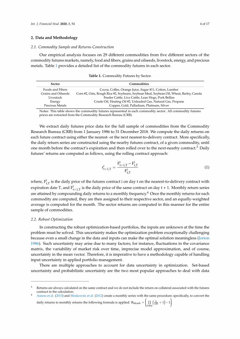
2.1. Commodity Sample and Returns Construction

Our empirical analysis focuses on 29 different commodities from five different sectors of thecommodity futures markets, namely, food and fibers, grains and oilseeds, livestock, energy, and preciousmetals. Table 1 provides a detailed list of the commodity futures in each sector.

Table 1. Commodity Futures by Sector.

Sector Commodities

Foods and Fibers Cocoa, Coffee, Orange Juice, Sugar #11, Cotton, LumberGrains and Oilseeds Corn #2, Oats, Rough Rice #2, Soybeans, Soybean Meal, Soybean Oil, Wheat, Barley, Canola

Livestock Feeder Cattle, Live Cattle, Lean Hogs, Pork BelliesEnergy Crude Oil, Heating Oil #2, Unleaded Gas, Natural Gas, Propane

Precious Metals Copper, Gold, Palladium, Platinum, Silver

Notes: This table shows the commodity futures represented in each commodity sector. All commodity futuresprices are extracted from the Commodity Research Bureau (CRB).

We extract daily futures price data for the full sample of commodities from the CommodityResearch Bureau (CRB) from 1 January 1986 to 31 December 2018. We compute the daily returns oneach future contract using either the nearest- or the next nearest-to-delivery contract. More specifically,the daily return series are constructed using the nearby futures contract, of a given commodity, untilone month before the contract’s expiration and then rolled over to the next-nearby contract.3 Dailyfutures’ returns are computed as follows, using the rolling contract approach:

rit+1,T =

Fit+1,T − Fi

t,T

Fit,T

(1)

where, Fit,T is the daily price of the futures contract i on day t on the nearest-to-delivery contract with

expiration date T, and Fit+1,T is the daily price of the same contract on day t + 1. Monthly return series

are attained by compounding daily returns to a monthly frequency.4 Once the monthly returns for eachcommodity are computed, they are then assigned to their respective sector, and an equally-weightedaverage is computed for the month. The sector returns are computed in this manner for the entiresample of commodities.

2.2. Robust Optimization

In constructing the robust optimization-based portfolios, the inputs are unknown at the time theproblem must be solved. This uncertainty makes the optimization problem exceptionally challengingbecause even a small change in the data and inputs can make the optimal solution meaningless (Jorion1986). Such uncertainty may arise due to many factors; for instance, fluctuations in the covariancematrix, the variability of market risk over time, imprecise model approximation, and of course,uncertainty in the mean vector. Therefore, it is imperative to have a methodology capable of handlinginput uncertainty in applied portfolio management.

There are multiple approaches to account for data uncertainty in optimization. Set-baseduncertainty and probabilistic uncertainty are the two most popular approaches to deal with data

3 Returns are always calculated on the same contract and we do not include the return on collateral associated with the futurescontract in the calculation.

4 Asness et al. (2013) and Moskowitz et al. (2012) create a monthly series with the same procedure; specifically, to convert the

daily returns to monthly returns the following formula is applied: RMonth =

∏i∈day

( ri100 + 1

)− 1

.

Int. J. Financial Stud. 2020, 8, 54 5 of 17

ambiguity in the optimization problem. Each of these techniques helps to obtain solutions that aregood for most realizations of data and provides immunization against the effect of data uncertainty.Under the set-based uncertainty models, it is assumed that the data belong to a set with differentconstraints without making any assumptions about the relative likelihood of the various data pointswithin that set (Goldfarb and Iyengar 2003; Tütüncü and Koenig 2004). We appeal to the probabilisticuncertainty approach that uses a probability distribution to account for different outcomes in the data(Kim et al. 2016).

Let rn be the n-dimensional random vector of returns with joint density P(r) and f(w, r) be afunction of decision vector w = (w1, w, . . .wn) where wi is the proportion of money invested in asseti and random vector of returns r. The expected value and the variance of the function f(w, r) aregiven by:

µ = E[f(w, r)] =∫

f(w, r)P(r)dr (2)

Σ = Var[f(w, r)] =∫

f(w, r)2 P(r)dr− E[f(w, r)]2 (3)

For a given confidence level α ∈ (0, 1), the conditional value-at-risk is defined as:

CVaRα(f(w, r)) =1

(1−α)

∫f(w,r)≥VaRα(f(w,r))

f(w, r)P(r)dr (4)

where, VaRα(f(w, r)) = min{γ : Pr(f(w, r) ≤ γ) ≥ α

}.

There are various approaches to uncertainty transmission in the mean, variance, and CVaRcalculations. We focus on Monte Carlo integration to approximate the values of these measures. Underthe Monte Carlo integration, we sample many scenarios for the uncertain data from a distribution thatcontains the possible values. For each sample, we estimate the values of the decision vector. If thereare m samples, then the expected value of the decision vector is:

w =1m

m∑i=1

ψ(zi) (5)

where, ψ(z) is some function of f(w, r).The primary benefit of robust portfolio optimization is that portfolios are formed by solving

optimization problems that are based on the classic mean-variance problem. Thus, robust optimizationis a simple extension aimed at achieving enhanced and more stable performance for mean-varianceinvestors. The standard Markowitz’s mean-variance optimization problem can be stated in thefollowing form:

minimizew

12

w′

Σw− θw′

µs.t. w′

1 = 1 (6)

where, θ ≥ 0 is the risk-aversion coefficient.Let us assume that the investor is facing the investment opportunity set where a riskless bond is

paying the risk-free rate (rrf). Then the portfolio expected return (µp) and volatility (σ2p) are given by:

µp = w′

(µ− rrf) + rrf and σ2p = w

′

Σw (7)

and the efficient portfolio can be obtained by maximizing the Sharpe ratio:

maxw

w′

(µ− rrf)√

w′Σws.t. w

′

1 = 1 (8)

where we impose the additional constraint that 0 ≤ wi ≤ 0.75 so as not to overweight a portfolio into agiven sector.

Int. J. Financial Stud. 2020, 8, 54 6 of 17

In addition to the Markowitz mean-variance optimization problem, a different approach thatminimizes the CVaR is very widely used by both academics and practitioners. The CVaR optimizationtechnique, which was proposed by Rockafellar and Uryasev (2000), does not depend on anydistributional assumptions for returns. Following Rockafellar and Uryasev (2000), CVaR can bedefined as follows:

minw, α

(α+1

(1−β)E(f(w, r) −α)+) (9)

where, α is the (1−β)-quantile of the loss distribution tail, (x)+ is x if x > 0 and 0 if x ≤ 0. The aboveproblem can be restated as a linear optimization problem by introducing auxiliary variables (zk), one foreach observation in the sample as follows:

minw,z,α

α+1

q(1−β)

q∑k=1

zks.t. wTrk + α+ zk ≥ 0 and zk ≥ 0 for k = 1, . . . , q (10)

where we similarly impose the additional constraint that 0 ≤ wi ≤ 0.75. An advantage of thisformulation is that it allows us to minimize the CVaR of a portfolio via linear programming.

2.3. Algorithms for Robust Optimization under Uncertainty

First, we calculate three different sets of a sample mean vector and covariance matrix usingeither the past 12, 15, or 18 months of historical returns. Second, we simulate 10,000 samples for eachlookback window using each sample mean vector and covariance matrix with 5000 observations. Third,we calculate the optimal commodity sector weights for each sample and estimate the weights vectorfor period t as the expected value of 10,000 simulation weights. Finally, we use this expected valueof the sectoral weights obtained in period t to invest in period t + 1. The portfolios are subsequentlyrebalanced every month on a rolling basis—that is, new optimal weights are calculated at the beginningof each month for each commodity sector. As discussed in Kim et al. (2017), investors utilizing robustportfolios will not rebalance with a high frequency since robust portfolios are less sensitive to changesin the market, and the aim is not to chase growth-potential assets aggressively.

The lookback, or estimation, period is a critical component to robust estimation. The lookbackrefers to how long historical data is used for parameter estimation when optimizing and re-optimizingthe portfolios each at the end of each holding period. We opt to use lookback periods of 12, 15,and 18 months to provide an adequate amount of observations to form the covariance matrix andestimate parameters.5 Our minimum monthly lookback period (12) is consistent with the lookbackperiod of 2 to 12 months of past returns established in the momentum literature, a signal which hasworked well out-of-sample over time and across geography (Asness et al. 2013).

2.4. Performance Metrics

Following the prior research of Kim et al. (2017), we identify several metrics to analyze theperformance of the commodity portfolios. Table 2 provides a summary and description of theperformance metrics used to analyze the risk and return features of the seven relevant portfolios—onenaïve buy-and-hold benchmark portfolio and six robust optimization-based portfolios formed frominvestment in five commodity sectors. We present and discuss our empirical findings in Section 3.

5 In fact, when the past 24 months of return data are used in the robust portfolio optimization process, both the MV and CVaRportfolios further underperform the naïve buy-and-hold benchmark.

Int. J. Financial Stud. 2020, 8, 54 7 of 17

Table 2. Performance Metrics.

Performance Metric Description

Arithmetic mean Reported as the average monthly return expressed as an annualized percentage.

Standard deviation Reported as the average monthly standard deviation expressed as an annualized percentage.

Geometric mean Reported as the average monthly return expressed as an annualized percentage.

Cumulative return Reported as the portfolio return over the full sample period.

Sample skewness Reported as a monthly average.

Sample excess kurtosis Reported as a monthly average.

Sharpe ratio Reported as the average excess monthly return divided by the monthly standard deviation, where the risk-freerate is obtained from Ken French’s website.

Tracking errorReported as the monthly average standard deviation of the difference between a commodity portfolio returns

and the value-weighted market index of returns from the Center for Research in Security Prices (CRSP).The CRSP market index return is obtained from Ken French’s website.

Information ratio Reported as the excess monthly return of a portfolio in excess of the CRSP value-weighted market index ofreturns divided by the tracking error.

CAPM alpha Reported as the average monthly alpha computed following Jensen (1968) expressed as an annualizedpercentage, where the market factor is obtained from Ken French’s website.

CAPM beta Reported as the average monthly beta computed following Sharpe (1964), where the market factor is obtainedfrom Ken French’s website.

Treynor ratio Reported as the average excess monthly return divided by the monthly portfolio beta, where the risk-free rate isobtained from Ken French’s website.

Sortino ratio Reported as the average excess monthly return divided by the monthly standard deviation of negative assetreturns, where the risk-free rate is obtained from Ken French’s website.

Historical 95% VaR Reported as the average expected 1-month loss with 95% certainty, based on historical returns.

Normal 95% VaR Reported as the average expected 1-month loss with 95% certainty, under normality.

Historical 95% CVaR Reported as the average expected 1-month loss beyond the VaR with 95% certainty, based on normality.

Normal 95% CVaR Reported as the average expected 1-month loss beyond the VaR with 95% certainty, based on historical returns.

M-squareReported as the average monthly return of a portfolio plus the product of the average monthly Sharpe ratio ofthe equally weighted benchmark and the average deviation of the standard deviation of the portfolio under

consideration from the benchmark portfolio.

Notes: This table shows the description of the performance metrics that are calculated for all commodity portfolios.The Ken French data library for the broad market and risk-free data can be found at https://mba.tuck.dartmouth.edu/pages/faculty/ken.french/data_library.html.

3. Results

3.1. Sectoral Risk and Returns Analysis

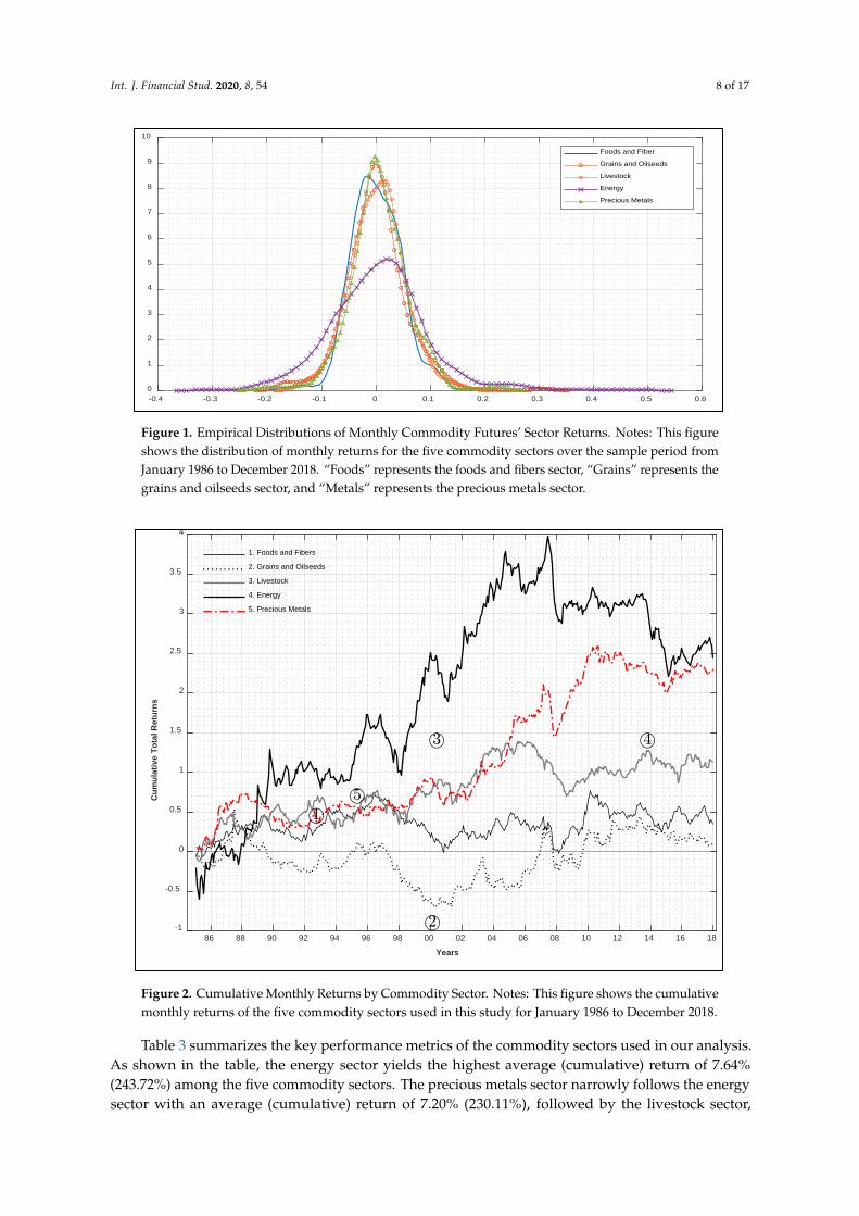
The underlying commodities we use in this study are diverse. Such diversity tends to manifestitself in smaller return correlations between constituents of different sectors rather than memberscategorized within the same sector (Adhikari and Putnam 2020). This heterogeneity can be viewedthrough the lens of distributional returns. Figure 1 plots the return distributions of the five commoditysectors. The energy sector exhibits a noticeable positive moderate skewness. The three other commoditysectors show little, if any, skewness. The foods and fibers, as well as livestock sectors, demonstrateslim, light tails (platykurtic) while the other return distributions more or less follow a standardnormal distribution. Finally, the varying “peakedness” of the sector distributions highlights thepotential usefulness of robust estimation in developing optimal portfolio allocations because of themarked dissimilarities.

Figure 2 provides additional insights into the return behavior of the commodity sectors. In terms ofcumulative total returns, the energy and precious metal sectors are the run-away winners. In contrast,the grains and oilseeds sectors are the worst performers during the sample period. Most of thecommodity sectors show favorable performance in the early-to-mid 2000s, followed by a sharpdownturn coinciding with the 2008 global financial crisis. Yet, it is apparent that the sectors do notcomove together strongly. An equally weighted investment in the five commodity sectors seeminglyyields obvious diversification benefits. However, the question we seek to answer is how the robustoptimization-based portfolios perform compared to such a naïve buy-and-hold benchmark composedof the same constituents.

Int. J. Financial Stud. 2020, 8, 54 8 of 17

Int. J. Financial Stud. 2020, 8, x 8 of 17

3. Results

3.1. Sectoral Risk and Returns Analysis

The underlying commodities we use in this study are diverse. Such diversity tends to manifest itself in smaller return correlations between constituents of different sectors rather than members categorized within the same sector (Adhikari and Putnam 2020). This heterogeneity can be viewed through the lens of distributional returns. Figure 1 plots the return distributions of the five commodity sectors. The energy sector exhibits a noticeable positive moderate skewness. The three other commodity sectors show little, if any, skewness. The foods and fibers, as well as livestock sectors, demonstrate slim, light tails (platykurtic) while the other return distributions more or less follow a standard normal distribution. Finally, the varying “peakedness” of the sector distributions highlights the potential usefulness of robust estimation in developing optimal portfolio allocations because of the marked dissimilarities.

Figure 1. Empirical Distributions of Monthly Commodity Futures’ Sector Returns. Notes: This figure shows the distribution of monthly returns for the five commodity sectors over the sample period from January 1986 to December 2018. “Foods” represents the foods and fibers sector, “Grains” represents the grains and oilseeds sector, and “Metals” represents the precious metals sector.

Figure 2 provides additional insights into the return behavior of the commodity sectors. In terms of cumulative total returns, the energy and precious metal sectors are the run-away winners. In contrast, the grains and oilseeds sectors are the worst performers during the sample period. Most of the commodity sectors show favorable performance in the early-to-mid 2000s, followed by a sharp downturn coinciding with the 2008 global financial crisis. Yet, it is apparent that the sectors do not comove together strongly. An equally weighted investment in the five commodity sectors seemingly yields obvious diversification benefits. However, the question we seek to answer is how the robust optimization-based portfolios perform compared to such a naïve buy-and-hold benchmark composed of the same constituents.

-0.4 -0.3 -0.2 -0.1 0 0.1 0.2 0.3 0.4 0.5 0.60

1

2

3

4

5

6

7

8

9

10

Foods and FIber

Grains and Oilseeds

Livestock

Energy

Precious Metals

Figure 1. Empirical Distributions of Monthly Commodity Futures’ Sector Returns. Notes: This figureshows the distribution of monthly returns for the five commodity sectors over the sample period fromJanuary 1986 to December 2018. “Foods” represents the foods and fibers sector, “Grains” represents thegrains and oilseeds sector, and “Metals” represents the precious metals sector.

Int. J. Financial Stud. 2020, 8, x 9 of 17

Figure 2. Cumulative Monthly Returns by Commodity Sector. Notes: This figure shows the cumulative monthly returns of the five commodity sectors used in this study for January 1986 to December 2018.

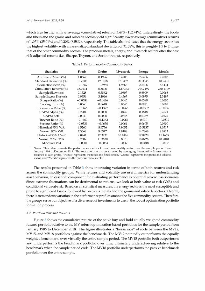
Table 3 summarizes the key performance metrics of the commodity sectors used in our analysis. As shown in the table, the energy sector yields the highest average (cumulative) return of 7.64% (243.72%) among the five commodity sectors. The precious metals sector narrowly follows the energy sector with an average (cumulative) return of 7.20% (230.11%), followed by the livestock sector, which lags further with an average (cumulative) return of 3.47% (112.74%). Interestingly, the foods and fibers and the grains and oilseeds sectors yield significantly lower average (cumulative) returns of 1.07% (35.01%) and 0.20% (6.58%), respectively. The table also indicates that the energy sector has the highest volatility with an annualized standard deviation of 31.38%; this is roughly 1.5 to 2 times that of the other commodity sectors. The precious metals, energy, and livestock sectors offer the best risk-adjusted returns (i.e., Sharpe, Treynor, and Sortino ratios), respectively.

The results presented in Table 3 show interesting variation in terms of both returns and risk across the commodity groups. While returns and volatility are useful metrics for understanding asset behavior, an essential component for evaluating performance is potential severe loss scenarios. Since extreme fluctuations can be detrimental to returns, we look at both value-at-risk (VaR) and conditional value-at-risk. Based on all statistical measures, the energy sector is the most susceptible and prone to significant losses, followed by precious metals and the grains and oilseeds sectors. Overall, there is tremendous variation in the performance profiles among the five commodity sectors. Therefore, the groups serve our objective of a diverse set of investments to use in the robust optimization portfolio formation process.

86 88 90 92 94 96 98 00 02 04 06 08 10 12 14 16 18

Years

-1

-0.5

0

0.5

1

1.5

2

2.5

3

3.5

4

Cum

ulat

ive

Tota

l Ret

urns

1. Foods and Fibers

2. Grains and Oilseeds

3. Livestock

4. Energy

5. Precious Metals

Figure 2. Cumulative Monthly Returns by Commodity Sector. Notes: This figure shows the cumulativemonthly returns of the five commodity sectors used in this study for January 1986 to December 2018.

Table 3 summarizes the key performance metrics of the commodity sectors used in our analysis.As shown in the table, the energy sector yields the highest average (cumulative) return of 7.64%(243.72%) among the five commodity sectors. The precious metals sector narrowly follows the energysector with an average (cumulative) return of 7.20% (230.11%), followed by the livestock sector,

Int. J. Financial Stud. 2020, 8, 54 9 of 17

which lags further with an average (cumulative) return of 3.47% (112.74%). Interestingly, the foodsand fibers and the grains and oilseeds sectors yield significantly lower average (cumulative) returnsof 1.07% (35.01%) and 0.20% (6.58%), respectively. The table also indicates that the energy sector hasthe highest volatility with an annualized standard deviation of 31.38%; this is roughly 1.5 to 2 timesthat of the other commodity sectors. The precious metals, energy, and livestock sectors offer the bestrisk-adjusted returns (i.e., Sharpe, Treynor, and Sortino ratios), respectively.

Table 3. Performance by Commodity Sector.

Statistics Foods Grains Livestock Energy Metals

Arithmetic Mean (%) 1.0662 0.1996 3.4703 7.6406 7.2003Standard Deviation (%) 15.7008 19.1108 17.0492 31.3845 18.2431

Geometric Mean (%) −0.1667 −1.5985 1.9863 2.6406 5.4434Cumulative Returns (%) 35.0131 6.5806 112.7373 243.7192 230.1109

Sample Skewness 0.1328 0.3862 0.0607 0.6909 0.0068Sample Excess Kurtosis 0.9356 3.1046 0.4567 3.0975 2.3497

Sharpe Ratio (%) −0.0384 −0.0446 0.0045 0.0390 0.0605Tracking Error (%) 0.0560 0.0648 0.0646 0.0971 0.0607

Information Ratio (%) −0.1466 −0.1377 −0.0966 −0.0302 −0.0539CAPM Alpha (%) 0.2201 0.2008 0.0442 0.1818 0.2621

CAPM Beta 0.0040 0.0008 0.0645 0.0339 0.0222Treynor Ratio (%) −0.1460 −0.1362 −0.0964 −0.0301 −0.0539Sortino Ratio (%) −0.0539 −0.0630 0.0064 0.0605 0.0900

Historical 95% VaR 6.5260 8.6736 7.9052 13.5137 8.0517Normal 95% VaR 7.3668 9.0577 7.8108 14.2868 8.0812

Historical 95% CVaR 9.0241 12.3231 10.1816 17.8220 11.4665Normal 95% CVaR 9.2607 11.3630 9.8673 18.0726 10.2818

M-Square (%) −0.0081 −0.0084 −0.0063 −0.0048 −0.0038

Notes: This table presents the performance metrics for each commodity sector over the sample period fromJanuary 1986 to December 2018. The sector returns are constructed by averaging the monthly futures returnsassigned to each group. “Foods” represents the foods and fibers sector, “Grains” represents the grains and oilseedssector, and “Metals” represents the precious metals sector.

The results presented in Table 3 show interesting variation in terms of both returns and riskacross the commodity groups. While returns and volatility are useful metrics for understandingasset behavior, an essential component for evaluating performance is potential severe loss scenarios.Since extreme fluctuations can be detrimental to returns, we look at both value-at-risk (VaR) andconditional value-at-risk. Based on all statistical measures, the energy sector is the most susceptible andprone to significant losses, followed by precious metals and the grains and oilseeds sectors. Overall,there is tremendous variation in the performance profiles among the five commodity sectors. Therefore,the groups serve our objective of a diverse set of investments to use in the robust optimization portfolioformation process.

3.2. Portfolio Risk and Returns

Figure 3 shows the cumulative returns of the naïve buy-and-hold equally weighted commodityfutures portfolio relative to the MV robust optimization-based portfolios for the sample period fromJanuary 1986 to December 2018. The figure illustrates a “horse race” of sorts between the MV12,MV15, and MV18 portfolios against the benchmark. The MV12 pointedly outperforms the equallyweighted benchmark, over virtually the entire sample period. The MV15 portfolio both outperformsand underperforms the benchmark portfolio over time, ultimately underachieving relative to thebenchmark when the sample period ends. The MV18 portfolio underperforms the passive benchmarkportfolio over the entire sample.

Int. J. Financial Stud. 2020, 8, 54 10 of 17Int. J. Financial Stud. 2020, 8, x 11 of 17

Figure 3. Performance of Equally Weighted and MV Optimization-based Commodity Portfolios. Notes: This figure shows the cumulative return for the naïve buy-and-hold benchmark portfolio relative to the mean-variance robust optimization-based portfolios over the sample period from January 1986 to December 2018. Equally weighted represents the naïve buy-and-hold benchmark portfolio. MV12, MV15, and MV18 represent the robust optimization-based mean-variance portfolios that use a 12-month, 15-month, and 18-month lookback period of returns, respectively, with a one-month portfolio holding period.

Similarly, Figure 4 shows a horse race for the CVaR optimization-based portfolios relative to the long-only naïve benchmark. The findings in relation to the lookback periods are quite similar to the mean-variance portfolios in Figure 3. The CVaR12 markedly outperforms the equally weighted benchmark. The CVaR15 portfolio over and underperforms the benchmark at various points over the sample period, ultimately falling short of the benchmark portfolio by the end of 2018. The CVaR18 portfolio consistently performs the worst of all robust optimization-based portfolios. However, unlike the MV18 portfolio, the CVaR18 portfolio performance tends to hug much closer to the 15-month look back portfolio (i.e., CVaR15) post-2008. Overall, it is apparent that the robust estimation procedure utilizing a 12-month lookback period performs far superior to the other portfolios conditioned on longer lookback periods.

Figure 4. Performance of Equally Weighted and CVaR Optimization-based Commodity Portfolios. Notes: This figure shows the cumulative return for the naïve buy-and-hold benchmark portfolio

86 88 90 92 94 96 98 00 02 04 06 08 10 12 14 16 18

Years

0

0.5

1

1.5

2

2.5

Cumu

lative

Retu

rns

MV12 Portfolio

Equally WeightedMV15 Portfolio

MV18 Portfolio

86 88 90 92 94 96 98 00 02 04 06 08 10 12 14 16 18

Years

0

0.5

1

1.5

2

2.5

Cumu

lative

Retur

ns

CVaR12 Portfolio

Equally WeightedCVaR15 Portfolio

CVaR18 Portfolio

Figure 3. Performance of Equally Weighted and MV Optimization-based Commodity Portfolios. Notes: This figure shows the cumulative return for the naïvebuy-and-hold benchmark portfolio relative to the mean-variance robust optimization-based portfolios over the sample period from January 1986 to December 2018.Equally weighted represents the naïve buy-and-hold benchmark portfolio. MV12, MV15, and MV18 represent the robust optimization-based mean-variance portfoliosthat use a 12-month, 15-month, and 18-month lookback period of returns, respectively, with a one-month portfolio holding period.

Int. J. Financial Stud. 2020, 8, 54 11 of 17

Similarly, Figure 4 shows a horse race for the CVaR optimization-based portfolios relative tothe long-only naïve benchmark. The findings in relation to the lookback periods are quite similar tothe mean-variance portfolios in Figure 3. The CVaR12 markedly outperforms the equally weightedbenchmark. The CVaR15 portfolio over and underperforms the benchmark at various points over thesample period, ultimately falling short of the benchmark portfolio by the end of 2018. The CVaR18portfolio consistently performs the worst of all robust optimization-based portfolios. However, unlikethe MV18 portfolio, the CVaR18 portfolio performance tends to hug much closer to the 15-month lookback portfolio (i.e., CVaR15) post-2008. Overall, it is apparent that the robust estimation procedureutilizing a 12-month lookback period performs far superior to the other portfolios conditioned onlonger lookback periods.

Table 4 summarizes the performance metrics for the benchmark portfolio and all the robustoptimization-based portfolios. Following standard practices in the commodity literature (Rad et al.2020; Bakshi et al. 2017; Erb and Harvey 2006; Miffre and Rallis 2007; Szymanowska et al. 2014),we compare the performance of the sophisticated robust optimization-based portfolios to the equallyweighted buy-and-hold benchmark. The average (cumulative) returns for the best-performing MV12and CVaR12 portfolios are the 4.72% (145.42%) and 4.69% (144.58%); in contrast, the returns for thebenchmark portfolio (EW) are 3.46% (107.21%). The annualized standard deviations of MV12 andCVaR12 are 15.59% and 15.55%, respectively. The benchmark portfolio, on the other hand, only has astandard deviation of 11.41%. The standard deviations of the 15- and 18-month lookback portfolios areall higher than their comparable 12-month counterpart, even though these portfolios have lower returns.

Given the disparity in return and risk measures between the MV12 and CVaR12 portfolios and theequally weighted benchmark portfolio, it is natural to compare risk-adjusted returns to see if, in fact,the outperformance of the 12-month lookback portfolios is simply due to increased portfolio risk.The risk-adjusted measures, namely the Sharpe, Treynor, and Sortino ratios, elucidate the superiorityof the MV12 and CVaR12 portfolios. In all cases, the risk-adjusted measures are superior to that ofthe benchmark portfolio. The same is not true of the 15- and 18-month look back portfolios. Hence,the outperformance of the MV12 and CVaR12 portfolios can be attributed to the optimal allocationsthrough robust estimation. These results are consistent with the findings of Zhang et al. (2017) whofind that a robust futures strategy outperforms a corresponding non-robust strategy in out-of-sampletests in the face of ambiguity aversion. We conclude that the performance of an equally weightedbenchmark portfolio is suboptimal compared to the MV12 and CVaR12 robust optimization portfolios.Our findings highlight the benefits of applying sophisticated, robust optimization while forming aportfolio consisting of commodity futures. This view has also recently found support within theresearch of Rad et al. (2020). They document the benefits of applying a sophisticated weighting schemeto enhance the performance of long-short commodity portfolios.

Int. J. Financial Stud. 2020, 8, 54 12 of 17

Int. J. Financial Stud. 2020, 8, x 11 of 17

Figure 3. Performance of Equally Weighted and MV Optimization-based Commodity Portfolios. Notes: This figure shows the cumulative return for the naïve buy-and-hold benchmark portfolio relative to the mean-variance robust optimization-based portfolios over the sample period from January 1986 to December 2018. Equally weighted represents the naïve buy-and-hold benchmark portfolio. MV12, MV15, and MV18 represent the robust optimization-based mean-variance portfolios that use a 12-month, 15-month, and 18-month lookback period of returns, respectively, with a one-month portfolio holding period.

Similarly, Figure 4 shows a horse race for the CVaR optimization-based portfolios relative to the long-only naïve benchmark. The findings in relation to the lookback periods are quite similar to the mean-variance portfolios in Figure 3. The CVaR12 markedly outperforms the equally weighted benchmark. The CVaR15 portfolio over and underperforms the benchmark at various points over the sample period, ultimately falling short of the benchmark portfolio by the end of 2018. The CVaR18 portfolio consistently performs the worst of all robust optimization-based portfolios. However, unlike the MV18 portfolio, the CVaR18 portfolio performance tends to hug much closer to the 15-month look back portfolio (i.e., CVaR15) post-2008. Overall, it is apparent that the robust estimation procedure utilizing a 12-month lookback period performs far superior to the other portfolios conditioned on longer lookback periods.

Figure 4. Performance of Equally Weighted and CVaR Optimization-based Commodity Portfolios. Notes: This figure shows the cumulative return for the naïve buy-and-hold benchmark portfolio

86 88 90 92 94 96 98 00 02 04 06 08 10 12 14 16 18

Years

0

0.5

1

1.5

2

2.5

Cumu

lative

Retu

rns

MV12 Portfolio

Equally WeightedMV15 Portfolio

MV18 Portfolio

86 88 90 92 94 96 98 00 02 04 06 08 10 12 14 16 18

Years

0

0.5

1

1.5

2

2.5

Cumu

lative

Retur

ns

CVaR12 Portfolio

Equally WeightedCVaR15 Portfolio

CVaR18 Portfolio

Figure 4. Performance of Equally Weighted and CVaR Optimization-based Commodity Portfolios. Notes: This figure shows the cumulative return for the naïvebuy-and-hold benchmark portfolio relative to the robust optimization-based portfolios over the sample period from January 1986 to December 2018. Equally weightedrepresents the naïve buy-and-hold benchmark portfolio. CVaR12, CVaR15, and CVar18 represent the robust optimization-based conditional value-at-risk portfoliosthat use a 12-month, 15-month, and 18-month lookback period of returns, respectively, with a one-month portfolio holding period.

Int. J. Financial Stud. 2020, 8, 54 13 of 17

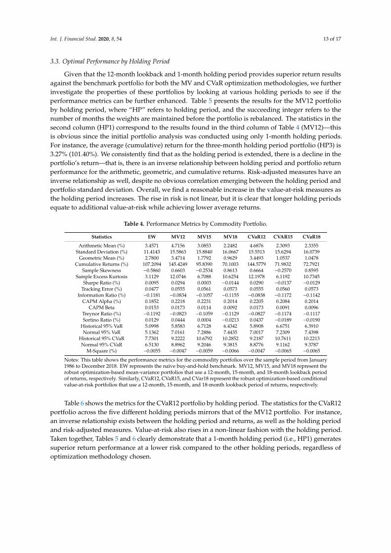
3.3. Optimal Performance by Holding Period

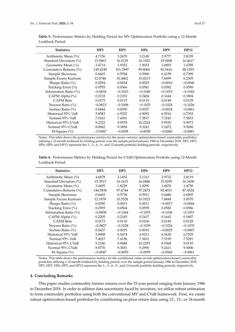
Given that the 12-month lookback and 1-month holding period provides superior return resultsagainst the benchmark portfolio for both the MV and CVaR optimization methodologies, we furtherinvestigate the properties of these portfolios by looking at various holding periods to see if theperformance metrics can be further enhanced. Table 5 presents the results for the MV12 portfolioby holding period, where “HP” refers to holding period, and the succeeding integer refers to thenumber of months the weights are maintained before the portfolio is rebalanced. The statistics in thesecond column (HP1) correspond to the results found in the third column of Table 4 (MV12)—thisis obvious since the initial portfolio analysis was conducted using only 1-month holding periods.For instance, the average (cumulative) return for the three-month holding period portfolio (HP3) is3.27% (101.40%). We consistently find that as the holding period is extended, there is a decline in theportfolio’s return—that is, there is an inverse relationship between holding period and portfolio returnperformance for the arithmetic, geometric, and cumulative returns. Risk-adjusted measures have aninverse relationship as well, despite no obvious correlation emerging between the holding period andportfolio standard deviation. Overall, we find a reasonable increase in the value-at-risk measures asthe holding period increases. The rise in risk is not linear, but it is clear that longer holding periodsequate to additional value-at-risk while achieving lower average returns.

Table 4. Performance Metrics by Commodity Portfolio.

Statistics EW MV12 MV15 MV18 CVaR12 CVAR15 CVaR18

Arithmetic Mean (%) 3.4571 4.7156 3.0853 2.2482 4.6876 2.3093 2.3355Standard Deviation (%) 11.4143 15.5863 15.8840 16.0667 15.5513 15.6294 16.0739

Geometric Mean (%) 2.7800 3.4714 1.7792 0.9629 3.4493 1.0537 1.0478Cumulative Returns (%) 107.2094 145.4249 95.8390 70.1003 144.5779 71.9832 72.7921

Sample Skewness −0.5860 0.6603 −0.2534 0.8613 0.6664 −0.2570 0.8595Sample Excess Kurtosis 3.1129 12.0746 6.7088 10.6254 12.1978 6.1192 10.7345

Sharpe Ratio (%) 0.0095 0.0294 0.0003 −0.0144 0.0290 −0.0137 −0.0129Tracking Error (%) 0.0477 0.0555 0.0561 0.0573 0.0555 0.0560 0.0573

Information Ratio (%) −0.1181 −0.0834 −0.1057 −0.1155 −0.0838 −0.1172 −0.1142CAPM Alpha (%) 0.1852 0.2218 0.2231 0.2014 0.2205 0.2084 0.2014

CAPM Beta 0.0153 0.0173 0.0114 0.0092 0.0173 0.0091 0.0096Treynor Ratio (%) −0.1192 −0.0823 −0.1059 −0.1129 −0.0827 −0.1174 −0.1117Sortino Ratio (%) 0.0129 0.0444 0.0004 −0.0213 0.0437 −0.0189 −0.0190

Historical 95% VaR 5.0998 5.8583 6.7128 6.4342 5.8908 6.6751 6.3910Normal 95% VaR 5.1362 7.0161 7.2886 7.4435 7.0017 7.2309 7.4398

Historical 95% CVaR 7.7301 9.2222 10.6792 10.2852 9.2187 10.7611 10.2213Normal 95% CVaR 6.5130 8.8962 9.2046 9.3815 8.8776 9.1162 9.3787

M-Square (%) −0.0055 −0.0047 −0.0059 −0.0066 −0.0047 −0.0065 −0.0065

Notes: This table shows the performance metrics for the commodity portfolios over the sample period from January1986 to December 2018. EW represents the naïve buy-and-hold benchmark. MV12, MV15, and MV18 represent therobust optimization-based mean-variance portfolios that use a 12-month, 15-month, and 18-month lookback periodof returns, respectively. Similarly, CVaR12, CVaR15, and CVar18 represent the robust optimization-based conditionalvalue-at-risk portfolios that use a 12-month, 15-month, and 18-month lookback period of returns, respectively.

Table 6 shows the metrics for the CVaR12 portfolio by holding period. The statistics for the CVaR12portfolio across the five different holding periods mirrors that of the MV12 portfolio. For instance,an inverse relationship exists between the holding period and returns, as well as the holding periodand risk-adjusted measures. Value-at-risk also rises in a non-linear fashion with the holding period.Taken together, Tables 5 and 6 clearly demonstrate that a 1-month holding period (i.e., HP1) generatessuperior return performance at a lower risk compared to the other holding periods, regardless ofoptimization methodology chosen.

Int. J. Financial Stud. 2020, 8, 54 14 of 17

Table 5. Performance Metrics by Holding Period for MV Optimization Portfolio using a 12-MonthLookback Period.

Statistics HP1 HP3 HP6 HP9 HP12

Arithmetic Mean (%) 4.7156 3.2670 3.2149 2.9777 2.8339Standard Deviation (%) 15.5863 16.2129 16.1022 15.9408 16.4617

Geometric Mean (%) 3.4714 1.9352 1.9033 1.6893 1.4789Cumulative Returns (%) 145.4249 101.3997 99.8060 92.5416 88.1293

Sample Skewness 0.6603 0.5784 0.5969 0.4159 0.7399Sample Excess Kurtosis 12.0746 10.4462 10.0213 7.6699 6.2305

Sharpe Ratio (%) 0.0294 0.0034 0.0025 −0.0016 −0.0040Tracking Error (%) 0.0555 0.0566 0.0561 0.0582 0.0589

Information Ratio (%) −0.0834 −0.1023 −0.1040 −0.1035 −0.1042CAPM Alpha (%) 0.2218 0.2333 0.2404 0.1644 0.1804

CAPM Beta 0.0173 0.0115 0.0110 0.0149 0.0129Treynor Ratio (%) −0.0823 −0.1008 −0.1025 −0.1024 −0.1026Sortino Ratio (%) 0.0444 0.0050 0.0037 −0.0024 −0.0061

Historical 95% VaR 5.8583 6.5522 6.9092 6.5516 6.7393Normal 95% VaR 7.0161 7.4301 7.3817 7.3243 7.5833

Historical 95% CVaR 9.2222 9.9578 10.2224 9.9530 9.9973Normal 95% CVaR 8.8962 9.3858 9.3241 9.2472 9.5690

M-Square (%) −0.0047 −0.0058 −0.0058 −0.0060 −0.0061

Notes: This table shows the performance metrics for the mean-variance optimization-based commodity portfoliosutilizing a 12-month lookback by holding period, over the sample period January 1986 to December 2018. HP1, HP3,HP6, HP9, and HP12 represent the 1-, 3-, 6-, 9-, and 12-month portfolio holding periods, respectively.

Table 6. Performance Metrics by Holding Period for CVaR Optimization Portfolio using 12-MonthLookback Period.

Statistics HP1 HP3 HP6 HP9 HP12

Arithmetic Mean (%) 4.6878 3.1452 3.1313 2.9732 2.8119Standard Deviation (%) 15.5513 16.1615 16.0486 15.9299 16.3438

Geometric Mean (%) 3.4495 1.8229 1.8290 1.6876 1.4750Cumulative Returns (%) 144.5836 97.6744 97.2473 92.4031 87.4524

Sample Skewness 0.6665 0.5738 0.5911 0.4486 0.6995Sample Excess Kurtosis 12.1978 10.5528 10.1023 7.8684 5.8570

Sharpe Ratio (%) 0.0290 0.0013 0.0011 −0.0017 −0.0044Tracking Error (%) 0.0555 0.0564 0.0559 0.0582 0.0586

Information Ratio (%) −0.0838 −0.1044 −0.1055 −0.1036 −0.1051CAPM Alpha (%) 0.2205 0.2345 0.2417 0.1643 0.1807

CAPM Beta 0.0173 0.0110 0.0106 0.0149 0.0128Treynor Ratio (%) −0.0827 −0.1028 −0.1039 −0.1024 −0.1035Sortino Ratio (%) 0.0437 0.0019 0.0016 −0.0025 −0.0067

Historical 95% VaR 5.8908 6.5674 6.9211 6.5630 6.7529Normal 95% VaR 7.0017 7.4156 7.3631 7.3195 7.5291

Historical 95% CVaR 9.2186 9.9688 10.2255 9.9368 9.9135Normal 95% CVaR 8.8776 9.3651 9.2990 9.2411 9.5006

M–Square (%) −0.0047 −0.0059 −0.0059 −0.0060 −0.0061

Notes: This table shows the performance metrics for the conditional value-at-risk optimization-based commodityportfolios utilizing a 12-month lookback by holding period, over the sample period January 1986 to December 2018.HP1, HP3, HP6, HP9, and HP12 represent the 1-, 3-, 6-, 9-, and 12-month portfolio holding periods, respectively.

4. Concluding Remarks

This paper studies commodity futures returns over the 33-year period ranging from January 1986to December 2018. In order to address data uncertainty faced by investors, we utilize robust estimationto form commodity portfolios using both the conventional MV and CVaR framework. First, we createrobust optimization-based portfolios by conditioning on prior return data using 12-, 15-, or 18-month

Int. J. Financial Stud. 2020, 8, 54 15 of 17

lookback periods to generate the covariance matrix. Next, we simulate the return-risk outcomes foreach lookback window using the respective sample mean vector and covariance matrix to create theoptimal portfolio weights for each commodity sector. Finally, the portfolios are held for one monthand are then recalibrated for the next one month holding period on a rolling basis. In total, we analyzethe performance metrics of three MV robust optimization-based portfolios over three lookback periodsand three CVaR robust optimization-based portfolios over the same three lookback periods.

The performance of the robust portfolios is compared against a naïve equally weightedbuy-and-hold benchmark portfolio of commodity futures. The results indicate that portfoliosconstructed using robust optimization with a 12-month lookback (MV12 and CVaR12) outperformboth the benchmark portfolio as well as the other robust optimization-based portfolios. These findingssuggest that the utility of historical returns beyond 12 months sharply deteriorates when used asinput in forming robust portfolio weights. Our findings are consistent with Kim et al. (2017) thatrobust optimization-based portfolios can offer returns well beyond what a passive benchmark canoffer. However, our findings are qualified, as only a lookback period of 12 months produces superiorrisk-adjusted returns. A more in-depth analysis of the holding period for the MV12 and CVarR12portfolios shows that the 1-month holding period is optimal. Overall, our findings suggest that thenaïve equally weighting scheme traditionally employed in commodity portfolio constructions can beenhanced by using the sophisticated, robust optimization technique.

The key contributions of this paper are to address data uncertainty faced by investors in thecommodity futures markets, evaluate the performance of robust-optimized portfolios against abuy-and-hold equally weighted portfolio, and examine the most informative lookback and holdingperiods in the commodity portfolio formation process. Our findings suggest that the naïve equallyweighted scheme traditionally employed in the portfolio formation process can be improved by theuse of a more sophisticated robust optimization technique. A practical implementation of robustoptimization in the financial markets may provide valuable benefits to investors. The methodologycan efficiently handle a class of interior-point optimizers that are capable of managing second-orderconstraints and can produce better weights than the classical mean-variance approach under uncertainty.Nonetheless, while risk-adjusted returns outperform a naïve benchmark, an implementation of thisapproach will have more value-at-risk for investors.

Author Contributions: All three authors spent equal amount of time and effort in completing this paper.All authors have read and agreed to the published version of the manuscript.

Funding: This research received no external funding.

Conflicts of Interest: The authors declare no conflict of interest.

References

Adhikari, Ramesh, and Kyle J. Putnam. 2020. Comovement in the Commodity Futures Markets: An Analysis ofthe Energy, Grains, and Livestock Sectors. Journal of Commodity Markets 18: 100090. [CrossRef]

Asness, Clifford S., Tobias J. Moskowitz, and Lasse Heje Pedersen. 2013. Value and Momentum Everywhere.Journal of Finance 68: 929–85. [CrossRef]

Bakshi, Gurdip, Xiaohui Gao, and Alberto G. Rossi. 2017. Understanding the Sources of Risk Underlying theCross Section of Commodity Returns. Management Science 65: 619–41. [CrossRef]

Best, Michael J., and Robert R. Grauer. 1991. On the Sensitivity of Mean-Variance-Efficient Portfolios to Changes inAsset Means: Some Analytical and Computational Results. Review of Financial Studies 4: 315–432. [CrossRef]

Bhardwaj, Geetesh, Gary Gorton, and K. Geert Rouwenhorst. 2015. Facts and Fantasies about Commodity Futures TenYears Later. NBER Working Paper Series; New York: National Bureau of Economic Research, Inc., pp. 1–29.

Bi, Junna, Hanqing Jin, and Qingbin Meng. 2018. Behavioral Mean-Variance Portfolio Selection. European Journalof Operational Research 271: 644–63. [CrossRef]

Black, Fischer, and Robert Litterman. 1992. Global Portfolio Optimization. Financial Analysts Journal 48: 28–43.[CrossRef]

Int. J. Financial Stud. 2020, 8, 54 16 of 17

Calafiore, Giuseppe C. 2007. Ambiguous Risk Measures and Optimal Robust Portfolios. SIAM Journal onOptimization 18: 853–77. [CrossRef]

Ceria, Sebastián, and Robert A. Stubbs. 2006. Incorporating Estimation Errors into Portfolio Selection: RobustPortfolio Construction. Journal of Asset Management 7: 109–27. [CrossRef]

DeMiguel, Victor, Lorenzo Garlappi, and Raman Uppal. 2009. Optimal versus Naive Diversification:How Inefficient Is the 1/N Portfolio Strategy? Review of Financial Studies 22: 1915–53. [CrossRef]

Elliott, Robert J., and Tak Kuen Siu. 2010. On Risk Minimizing Portfolios under a Markovian Regime-SwitchingBlack-Scholes Economy. Annals of Operations Research 176: 271–91. [CrossRef]

Erb, Claude B., and Campbell R. Harvey. 2006. The Strategic and Tactical Value of Commodity Futures. FinancialAnalysts Journal 62: 125–78. [CrossRef]

Fan, Jianqing, Yingying Fan, and Jinchi Lv. 2008. High Dimensional Covariance Matrix Estimation Using a FactorModel. Journal of Econometrics 147: 186–97. [CrossRef]

Goldfarb, Donald, and Garud Iyengar. 2003. Robust Portfolio Selection Problems. Mathematics of OperationsResearch 28: 1–38. [CrossRef]

Gorton, Gary, and K. Geert Rouwenhorst. 2006. Facts and Fantasies about Commodity Futures. Financial AnalystsJournal 62: 47–68. [CrossRef]

Grauer, Robert R., and Frederick C. Shen. 2000. Do Constraints Improve Portfolio Performance? Journal of Bankingand Finance 24: 1253–74. [CrossRef]

Green, Richard C., and Burton Hollifield. 1992. When Will Mean-Variance Efficient Portfolios Be Well Diversified?The Journal of Finance 47: 1785–809. [CrossRef]

Huang, Xiaoxia, and Tingting Yang. 2020. How Does Background Risk Affect Portfolio Choice: An AnalysisBased on Uncertain Mean-Variance Model with Background Risk. Journal of Banking and Finance 111: 105726.[CrossRef]

Huo, Lijuan, Tae-Hwan Kim, and Yunmi Kim. 2012. Robust Estimation of Covariance and Its Application toPortfolio Optimization. Finance Research Letters 9: 121–34. [CrossRef]

Jensen, Michael C. 1968. Problems in the Selection of Security Portfolios—The Performance of Mutual Funds inthe Period 1945–1964. Journal of Finance 23: 389–416. [CrossRef]

Jorion, Philippe. 1986. Bayes-Stein Estimation for Portfolio Analysis. The Journal of Financial and QuantitativeAnalysis 21: 279–92. [CrossRef]

Kim, Tae-Hwan, and Halbert White. 2004. On More Robust Estimation of Skewness and Kurtosis. Finance ResearchLetters 1: 56–73. [CrossRef]

Kim, Jang Ho, Woo Chang Kim, and Frank J. Fabozzi. 2013. Composition of Robust Equity Portfolios. FinanceResearch Letters 10: 72–81. [CrossRef]

Kim, Woo Chang, Jang Ho Kim, and Frank J. Fabozzi. 2016. Robust Equity Portfolio Management + Website:Formulations, Implementations and Properties Using MATLAB, 1st ed. Hoboken: John Wiley & Sons, Inc.

Kim, Jang Ho, Woo Chang Kim, Do-Gyun Kwon, and Frank J. Fabozzi. 2017. Robust Equity Portfolio Performance.Annals of Operations Research 266: 293–312. [CrossRef]

Lim, Andrew E. B., Jeyaveerasingam George Shanthikumar, and Gah-Yi Vahn. 2011. Conditional Value-at-Risk inPortfolio Optimization: Coherent but Fragile. Operations Research Letters 39: 163–71. [CrossRef]

Lwin, Khin T., Rong Qu, and Bart L. MacCarthy. 2017. Mean-VaR Portfolio Optimization: A NonparametricApproach. European Journal of Operational Research 260: 751–66. [CrossRef]

Markowitz, Harry. 1952. Portfolio Selection. The Journal of Finance 7: 77–91.Michaud, Richard O. 1998. Efficient Asset Management: A Practical Guide to Stock Portfolio Optimization and Asset

Allocation. Boston: Oxford University Press.Michaud, Richard O., and Robert Michaud. 2008. Estimation Error and Portfolio Optimization: A Resampling

Solution. Journal of Investment Management 6: 8–28. [CrossRef]Miffre, Joëlle, and Georgios Rallis. 2007. Momentum Strategies in Commodity Futures Markets. Journal of Banking

and Finance 31: 1863–86. [CrossRef]Moskowitz, Tobias J., Yao Hua Ooi, and Lasse Heje Pedersen. 2012. Time Series Momentum. Journal of Financial

Economics 104: 228–50. [CrossRef]Natarajan, Karthik, Dessislava Pachamanova, and Melvyn Sim. 2009. Constructing Risk Measures from Uncertainty

Sets. Operations Research 57: 1129–41. [CrossRef]

Int. J. Financial Stud. 2020, 8, 54 17 of 17

Post, Thierry, Selçuk Karabatı, and Stelios Arvanitis. 2019. Robust Optimization of Forecast Combinations.International Journal of Forecasting 35: 910–26. [CrossRef]

Rad, Hossein, Rand Kwong Yew Low, Joëlle Miffre, and Robert Faff. 2020. Does Sophistication of the WeightingScheme Enhance the Performance of Long-Short Commodity Portfolios? Journal of Empirical Finance 58:164–80. [CrossRef]

Rockafellar, Ralph Tyrrell, and Stanislav Uryasev. 2000. Optimization of Conditional Value-at-Risk. The Journal ofRisk 2: 21–41. [CrossRef]

Scherer, Bernd. 2007. Can Robust Portfolio Optimisation Help to Build Better Portfolios? Journal of AssetManagement 7: 374–87. [CrossRef]

Sharpe, William F. 1964. Capital Asset Prices: A Theory of Market Equilibrium Under Conditions of Risk.The Journal of Finance 19: 425–42.

Shen, Ruijun, and Shuzhong Zhang. 2008. Robust Portfolio Selection Based on a Multi-Stage Scenario Tree.European Journal of Operational Research 191: 864–87. [CrossRef]

Szymanowska, Marta, Frans de Roon, Theo Nijman, and Rob van den Goorbergh. 2014. An Anatomy ofCommodity Futures Risk Premia. Journal of Finance 69: 453–82. [CrossRef]

Tütüncü, Reha H., and Mark Koenig. 2004. Robust Asset Allocation. Annals of Operations Research 132: 157–87.[CrossRef]

Zakamulin, Valeriy. 2017. Superiority of Optimized Portfolios to Naive Diversification: Fact or Fiction? FinanceResearch Letters 22: 122–28. [CrossRef]

Zhang, Jinqing, Zeyu Jin, and Yunbi An. 2017. Dynamic Portfolio Optimization with Ambiguity Aversion.Journal of Banking and Finance 79: 95–109. [CrossRef]

Zhu, Shushang, and Masao Fukushima. 2009. Worst-Case Conditional Value-at-Risk with Application to RobustPortfolio Management. Operations Research 57: 1155–68. [CrossRef]

© 2020 by the authors. Licensee MDPI, Basel, Switzerland. This article is an open accessarticle distributed under the terms and conditions of the Creative Commons Attribution(CC BY) license (http://creativecommons.org/licenses/by/4.0/).