Informatic

a—

Univ

ersi

teit

van

Amst

erdam

Supervisor(s): Dr. Robert G. Belleman (UvA) dr. Dick vanAlbada (UvA)

Signed:

Robust touch detection and track-ing on the UvA Multi-Touch Table

Sander van Noort

June 16, 2009

Bachelor Informatica

Universiteit van Amsterdam

2

Abstract

This paper describes the application of the Kalman filter to a multi-touch table. The goal is toimprove the detection and tracking software of the table and making it more robust.

In this project we will do measurements to compare the old situation with the new situation.The measurements include both system and user performance. Measuring the user performanceis done by letting a group of test persons perform a set of tasks.

Contents

1 Introduction 3

2 Mutli-touch table and software 42.1 Table and hardware . . . . . . . . . . . . . . . . . . . . . . . . . . . . . . . . . . 42.2 Detection and processing . . . . . . . . . . . . . . . . . . . . . . . . . . . . . . . . 5

2.2.1 Touchlib . . . . . . . . . . . . . . . . . . . . . . . . . . . . . . . . . . . . . 52.2.2 OSC . . . . . . . . . . . . . . . . . . . . . . . . . . . . . . . . . . . . . . . 6

3 Theoritical background 73.1 The Kalman filter . . . . . . . . . . . . . . . . . . . . . . . . . . . . . . . . . . . 7

3.1.1 System model . . . . . . . . . . . . . . . . . . . . . . . . . . . . . . . . . . 73.1.2 The Discrete Kalman Filter Algorithm . . . . . . . . . . . . . . . . . . . . 7

3.2 Example . . . . . . . . . . . . . . . . . . . . . . . . . . . . . . . . . . . . . . . . . 83.3 Blobs . . . . . . . . . . . . . . . . . . . . . . . . . . . . . . . . . . . . . . . . . . 93.4 Simulation in Matlab . . . . . . . . . . . . . . . . . . . . . . . . . . . . . . . . . . 9

3.4.1 Generated data . . . . . . . . . . . . . . . . . . . . . . . . . . . . . . . . . 9

4 Design and Implementation 114.1 Kalman filter . . . . . . . . . . . . . . . . . . . . . . . . . . . . . . . . . . . . . . 114.2 Tracker . . . . . . . . . . . . . . . . . . . . . . . . . . . . . . . . . . . . . . . . . 114.3 Applications . . . . . . . . . . . . . . . . . . . . . . . . . . . . . . . . . . . . . . . 12

5 Experiments 135.1 System Performance . . . . . . . . . . . . . . . . . . . . . . . . . . . . . . . . . . 135.2 User performance . . . . . . . . . . . . . . . . . . . . . . . . . . . . . . . . . . . . 13

6 Conclusion 176.1 Kalman filter performance . . . . . . . . . . . . . . . . . . . . . . . . . . . . . . . 176.2 Future work . . . . . . . . . . . . . . . . . . . . . . . . . . . . . . . . . . . . . . . 17

Appendices 19.1 Hardware . . . . . . . . . . . . . . . . . . . . . . . . . . . . . . . . . . . . . . . . 19.2 Configuration settings . . . . . . . . . . . . . . . . . . . . . . . . . . . . . . . . . 19

.2.1 TouchLib . . . . . . . . . . . . . . . . . . . . . . . . . . . . . . . . . . . . 19

.2.2 Kalman tracker . . . . . . . . . . . . . . . . . . . . . . . . . . . . . . . . . 20

2

CHAPTER 1

Introduction

Multi-touch displays allow users to interact directly on-screen using multiple fingers. Todaymulti-touch is becoming more and more popular and we see a lot of multi-touch products ap-pearing. Most modern computers are equipped with a mouse and keyboard or they have asingle-touch screen. These devices only allow to control one pointer on screen. Multi-touchbrings multiple pointers on screen and each pointer can be controlled independently. The userexperience with applications like photo browsers and games can be improved this way.

The Scientific Visualization and Virtual Reality group of the Section Computational Science(SCS) has constructed a Multi-Touch table. This table is being used for various research projects.A projector is used to display the image on the table surface and a camera is used to detecttouches.

The current detection and tracking software of the table still is very sensitive and prone toerrors. The tracking of fingers might be lost because of noise or in some cases because the positionof a detected finger might be too far off. These errors are in most cases caused by changes inlighting around the table. Our goal is to improve the detection and tracking software and makeit more robust.

In this research project we will focus only on improving the detection and tracking by applyinga Kalman filter to the raw measurement data for the touch positions generated by the imageprocessing stage. This means we leave the image processing alone. The Kalman filter gives anew estimate based on the previous estimate, a mathematical model and a new measurement.

We will build a few applications using the Kalman filter. Challenges are to keep the perfor-mance of the software high enough to process all touches within a frame period and to measurethe improvements compared to the old software.

3

CHAPTER 2

Multi-touch table and software

The multi-touch table used in this research project was constructed by L.Y.L. Muller in thecontext of his MSc research project with help of Paul Melis, Edwin Steffens and Robert Belleman[6]. An overview of the table and hardware will follow here. Then we will describe the videoprocessing and tracking.

2.1 Table and hardware

The Multi-touch table is constructed in a way that allows multiple users to collaboratively solvetasks. For this reason, the table is a horizontal multi-touch panel, allowing multiple users tointeract with the table in a natural manner. The dimensions of the table are 120 cm x 90 cm x80 cm (LxWxH), while the actual projection surface is 94.7 x 72.5 cm (LxW).

The table surface is semi-transparent and a projector is placed below the table surface.Important properties of the projector are the throwing distance and the required resolution. Thethrowing distance must be short enough to fit inside the table. Most common projectors cannotmeet this requirement. The selected projector for this table is the Mitsubishi XD500 U-ST. Thisdigital projector has a resolution of 1024 x 768 pixels and is capable of projecting a screen sizewith a diagonal of 102 cm from a distance of 50 cm. A mirror is used to project the screen onthe table surface (figure 2.1).

To detect touches a camera is placed below the table surface, combined with a techniquecalled rear-side illumination (figure 2.2). Rear-side illumination is a variant of the diffusedillumination technique. A diffuser is attached to the rear side of the table surface. Then insidethe table multiple infrared light illuminators are pointed straight at the diffuser. Part of the lightwill be diffused, while the other part passes through the material. When a fingertip is placed onthe surface, it will reflect light allowing blobs to be detected by the camera. The camera used isthe Firefly MV, capable of 60 frames per second at a resolution of 640 x 480 pixels.

2.2 Detection and processing

To detect and process touches software is required. Several frameworks for Multi-Touch detectionand processing are available. The framework used for this multi-touch table is Touchlib.

2.2.1 Touchlib

Touchlib is an open-source library for creating multi-touch interacting devices and is developedby the NUI group [2]. Touchlib takes care of the video processing, blob detection and tracking.The video processing in touchlib is done through OpenCV, a library aimed at real time computervision [3].

4

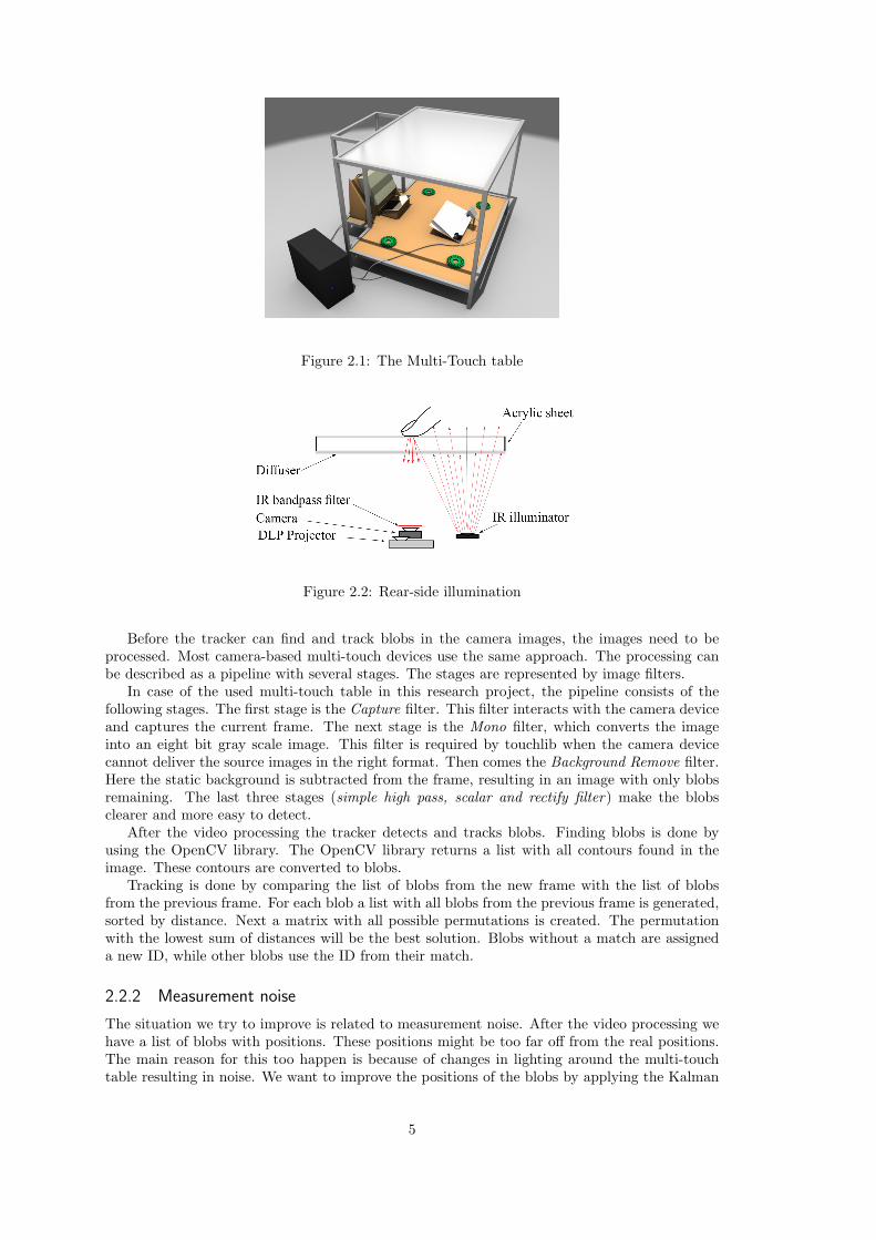
Figure 2.1: The Multi-Touch table

Figure 2.2: Rear-side illumination

Before the tracker can find and track blobs in the camera images, the images need to beprocessed. Most camera-based multi-touch devices use the same approach. The processing canbe described as a pipeline with several stages. The stages are represented by image filters.

In case of the used multi-touch table in this research project, the pipeline consists of thefollowing stages. The first stage is the Capture filter. This filter interacts with the camera deviceand captures the current frame. The next stage is the Mono filter, which converts the imageinto an eight bit gray scale image. This filter is required by touchlib when the camera devicecannot deliver the source images in the right format. Then comes the Background Remove filter.Here the static background is subtracted from the frame, resulting in an image with only blobsremaining. The last three stages (simple high pass, scalar and rectify filter) make the blobsclearer and more easy to detect.

After the video processing the tracker detects and tracks blobs. Finding blobs is done byusing the OpenCV library. The OpenCV library returns a list with all contours found in theimage. These contours are converted to blobs.

Tracking is done by comparing the list of blobs from the new frame with the list of blobsfrom the previous frame. For each blob a list with all blobs from the previous frame is generated,sorted by distance. Next a matrix with all possible permutations is created. The permutationwith the lowest sum of distances will be the best solution. Blobs without a match are assigneda new ID, while other blobs use the ID from their match.

2.2.2 Measurement noise

The situation we try to improve is related to measurement noise. After the video processing wehave a list of blobs with positions. These positions might be too far off from the real positions.The main reason for this too happen is because of changes in lighting around the multi-touchtable resulting in noise. We want to improve the positions of the blobs by applying the Kalman

5

Figure 2.3: Several image filters

filter.

2.2.3 OSC

OSC is an application for touchlib that transmits touch data to other applications. The touchdata are transmitted using the TUIO protocol. TUIO is an open framework which defines acommon protocol and API for multi-touch surfaces [1]. The advantage of using this applicationis when touchlib changes, only this application needs to be recompiled. Other applications usingTUIO can benefit without being recompiled.

For this reason, we will create a custom version of OSC using the Kalman filter. In that caseany application which receives TUIO packages can take advantage of the Kalman filter.

6

CHAPTER 3

Theoretical background

3.1 The Kalman filter

The Kalman filter is a recursive solution to the discrete-data linear filtering problem, describedby R.E. Kalman [4]. A good introduction about Kalman filtering can be found in Chapter one ofStochastic Models, Estimation, and Control (Maybeck, 1979) [5] and in An Introduction to theKalman Filter (Greg Welch and Gary Bishop, 2006) [8].

The Kalman filter is a set of mathematical equations which can estimate the state of aprocess, in a way that it minimizes the mean of the squared error. One of the big advantages ofthe Kalman filter is that no history of observations and estimates is required.

3.1.1 System model

The Kalman filter assumes the state of the system is represented as a vector xk. The Kalmanfilter assumes that the underlying systems is linear and thus that its evolution can be describedby equation (3.1). This we call the true state. Equation (3.2) describes how we observe the truestate. This we call the observed state.

xk = Akxk−1 + Bkuk + wk (3.1)

zk = Hkxk + vk (3.2)

Ak is the state transition model (n × n matrix) which is applied to the previous state. Bk

(n× n matrix) is the control-input model which is applied to the control vector uk. The n×mmatrix H maps the true state space into the observed state space.

The random vectors wk and vk represent the process and measurement noise. These vectorsare assumed to be independent and zero mean Gaussian white noise. The noise vectors have thefollowing normal distributions:

vk = N(0, Q) (3.3)

wk = N(0, R) (3.4)

Here Q and R are n× n covariance matrices.

3.1.2 The Discrete Kalman Filter Algorithm

There are two distinct phases in the Kalman filter algorithm, namely the predict and updatephase. The predict phase calculates the new estimate by using the previous estimate. Next theupdate phase ’corrects’ the predicted estimate by weighting it against the measurement of that

7

time step. In case there is more than one measurement the update phase can be applied multipletimes for one time step.

Predict phase:xk = Axk−1 + Bu (3.5)

Pk = APk−1AT + Q (3.6)

In equation (3.5) the new state is predicted by applying the state transition model to theprevious state. Then in equation (3.6) the error covariance matrix is updated.

Update phase:K = PkHT (HPkHT + R)−1; (3.7)

xk = xk + K(z −Hxk) (3.8)

Pk = Pk −KHPk (3.9)

In equation (3.7) the gain matrix K is calculated. The next two equations (3.8) and (3.9)update the state estimate and error covariance matrix by incorporating the measurement vectorzk and gain matrix K.

3.2 Example

We give an example to clarify the concept of the Kalman filter. We take a voltmeter measuring12 volts. The process model assumes the voltage is constant with noise added. This will give usthe following equations:

xk = xk−1 + wk (3.10)

zk = xk + vk (3.11)

The process evolves according to equation (3.10) and the measurements are yielded accordingto equation (3.11). Both equations have random noise added. We will assume the process modelhas an uncertainty (variance) of 12 and the measurements an uncertainty of 22. We can ignorethe control input matrices and the observation matrix is simply 1. This will result in the followingplot in matlab:

Figure 3.1: Voltmeter example

As can be seen the filtered values are a lot closer to the true values.

8

3.3 Blobs

In this section we describe how the Kalman filter is applied to the blobs and also describe therequired matrices for the model. A blob is a finger being tracked on the multi-touch table. Wehave chosen to describe a blob by its position, velocity and acceleration. This results in thefollowing state vector:

x =

xy

xvelyvelxaccyacc

(3.12)

The state vector has a 6×6 error covariance matrix P . This matrix describes the uncertaintyof the variables. Since we do not know the velocity and acceleration after the first measurement,the error covariance matrix should be initialized with high values.

The state evolves by applying the transition matrix. The transition model matrix will be:

A =

1 0 dt 0 1/2 ∗ dt2 00 1 0 dt 0 1/2 ∗ dt2

0 0 1 0 dt 00 0 0 1 0 dt0 0 0 0 1 00 0 0 0 0 1

(3.13)

The time step is represented by dt. The new position of the next time step depends onthe speed and acceleration. The new speed depends on the acceleration. The acceleration isassumed to be constant in this model. This is not true since a finger on the multi-touch tablecan change direction or change acceleration very quickly. For this reason, the process noise forthe acceleration should be reasonable high. The process noise is described by a 6× 6 covariancematrix Q and is constant.

The true state is mapped into the observation space. We can only observe the position of afinger, not the velocity and acceleration. This means the observation matrix is:

H =(

1 0 0 0 0 00 1 0 0 0 0

)(3.14)

Finally the measurement noise is described by a 2×2 covariance matrix R. The values of thismatrix depends on the settings of the multi-touch table.

3.4 Simulation in Matlab

To gain more knowledge of the behavior of the Kalman filter we simulated the filter in Matlab[7]. We loaded a list of measurements from a file and applied the Kalman filter on the data. Weused simulated data as input.

3.4.1 Generated data

We have generated data for three different movements: a straight line from left to right, a circleand a sinusoidal movement pattern. All three movements have a constant velocity. We addednoise to the data and applied the Kalman filter. The purpose of using generated data is to showthe behavior of the Kalman filter for different movements. The advantage is that we know thetrue positions of the blobs, which is difficult to obtain for real data. This way we can analyzethe improvement of the estimated value.

We tested the data with different settings for the Kalman filter. The measurement noisecovariance matrix is kept the same all the time and we used four different process noise covariance

9

Average true value and observation differenceType Q1 Q2 Q3 Q4line 1.159855circle 1.342946sine 1.261719

Average true value and estimate differenceline 0.514984 0.682410 0.891342 0.925290circle 2.347459 0.843401 1.028913 1.075803sine 66.462975 8.258686 1.446208 1.330314

Table 3.1: Generated data results

matrices, varying from very low process noise to very high. The used values represent pixels fromthe camera of the multi-touch table. The table is represented by a field of 640 × 480 pixels.

R =(

32 00 32

)(3.15)

Q1 =

0 0 0 0 0 00 0 0 0 0 00 0 0 0 0 00 0 0 0 0 00 0 0 0 52 00 0 0 0 0 52

Q2 =

0 0 0 0 0 00 0 0 0 0 00 0 0 0 0 00 0 0 0 0 00 0 0 0 502 00 0 0 0 0 502

(3.16)

Q3 =

0 0 0 0 0 00 0 0 0 0 00 0 0 0 0 00 0 0 0 0 00 0 0 0 5002 00 0 0 0 0 5002

Q4 =

0 0 0 0 0 00 0 0 0 0 00 0 502 0 0 00 0 0 502 0 00 0 0 0 5002 00 0 0 0 0 5002

(3.17)

We used the filtered data to calculate the average of the differences between the estimatedvalues and true values. We also calculated the average between the measurement values and truevalues. See table 3.1 for the results.

Q1 shows a good improvement for the line movement, but the sinusoidal movement becomesmuch worse. This can be explained by the low process noise and the transition model. Thetransition model says the acceleration stays the same all the time and because the process noiseis very low, it will not change fast over time. This works in case of a straight line, but with afinger movement like a sinusoidal pattern it goes wrong.

The other three show better results for the circle and sinusoidal movement, but becausethe process noise is becoming much higher the advantage of the Kalman filter is disappearing.Because the measurement noise added to the generated data is already pretty low, it is difficultto get a significant improvement.

Figure 3.2: Plots of the filtered data for Q3

10

CHAPTER 4

Design and Implementation

The design and implementation has two core parts: the Kalman filter and the tracker. All codeis written in C++ on windows XP.

4.1 Kalman filter

The implementation of the Kalman filter is relative simple since the actual algorithm is only fivelines of matrix calculations. This means if a matrix class is present, the algorithm can almost betranslated one-on-one in code. Furthermore we need to run a Kalman filter for each blob thatis being tracked. For this reason, the Kalman filter is implemented as a class allowing multipleinstances to be created. A short version of the header follows here.

c l a s s Kalman {Kalman( s e t up i n f o ) ;

void p r ed i c t ( ) ;void update ( ) ;void applyKalman ( ) ;

void setObservat ion ( zx , zy ) ;void setEst imate ( xest , yest , vxest , vyest , axest , ayest ) ;Matrix getEst imate ( ) { re turn x ; }

}

When creating a new instance, the Kalman filter gets a structure filled with information aboutthe measurement and process noise covariance matrices. applyKalman runs the full algorithm,while predict and update only run their phases of the Kalman algorithm. This way if there areno measurements the filter can still predict the positions of the blobs. When there is more thanone measurement for a time step it can update multiple times.

4.2 Tracker

One of the goals of the Kalman filter is to improve the tracking. A tracker is an important partof a Multi-Touch system. To make Multi-Touch possible multiple fingers need to be identifiedand followed. A tracker will assign unique ID numbers to fingers and follow them over time.

Tracking is done by comparing the blobs of the new frame with the ones from the previousframe. The positions of the blobs of the new frame do not have their Kalman filter applied yetsince we do not know which Kalman filter of the previous frame belongs to the blob of the newframe.

To solve this problem we will apply the Kalman filter of the blob from the previous frame foreach blob of the new frame. Then we compare the estimated positions of these blobs.

This introduces a new problem. The default touchlib tracker builds for each blob in the newframe a list of all blobs from the previous frame sorted on distance. This means that we need to

11

apply the Kalman filter many times. For example, if we are tracking 10 blobs, this means thatwe need to apply the Kalman filter 100 times, which slows down everything dramatically.

To solve this performance problem we will first map the blobs onto a grid. Then we onlyconsider the blobs from the blob’s own cell and from the neighbor cells. The size of a cell shouldat least be big enough that a blob can never travel more than two cells within one frame period.With this design we only have to compare blobs to a few other blobs from the previous frame.

Apart from applying the Kalman filter to give better estimations of the positions, we alsouse the Kalman filter to recover from missing detections. Sometimes a blob disappears for a fewframes, while the finger was still on the table. To solve this problem we track the blob for a fewmore frames even while there are no measurements. The Kalman filter is used to predict theposition. When the blob appears again, tracking continues. Otherwise the blob disappears.

4.3 Applications

To demonstrate, use and test the Kalman filter and tracker two applications have been made.The first one, Kalman debug, is a simple application which draws the blobs and filtered paths.It is also able to show the grid, which the tracker uses to match blobs. The second application,OSC Kalman, is a modified version of OSC. Instead of the default tracker it uses the new tracker.This way any application that receives TUIO events can use the new tracker, without the needfor being recompiled.

12

CHAPTER 5

Experiments

We will show the results of two types of experiments. The first experiment measures the executionspeed of the trackers. We compare the default tracker of touchlib and the new tracker withKalman filtering.

The second experiment measures the improvement in user experience with the trackers. Agroup of test persons is used for this test.

5.1 System Performance

Adding the Kalman filter in the tracker slows down the tracker. Each blob of the previous framehas to apply the Kalman filter to all its neighbors. The framerate of the camera is 60 frames persecond. This means each iteration must be below (1/60) seconds.

The measurements are done by building a custom TouchLib library with timers placed in thefilter and tracker functions. The timer function used is QueryPerformanceCounter(), part of theWindows API. The average is calculated over 600 frames.

The ten active blobs performance measurement is done by placing two hands on the table.See Table 5.1 for the results.

As expected for zero blobs both trackers show nearly the same results as expected. Since onlythe trackers are different and there are no blobs to track, both trackers have nothing to do. Thefive, ten and forty blobs tests show a minor increase for the old tracker in average time and amajor increase for the new tracker. Five blobs are still acceptable for the new tracker, but whenmore than 10 blobs are active the average time is above 16.7ms. This means the blobs cannotbe processed within a frame period anymore.

The difference is likely because the new tracker needs to map the blobs onto a grid and applythe Kalman filters to all neighbors. The old tracker only has to build a list with nearest blobsand pick the nearest. Since we only have ten blobs this does not affect the performance thatmuch.

5.2 User performance

User performance is measured by letting test persons perform three different tasks. Each taskis executed two times: one time with the touchlib default tracker and one time with the newtracker. The order in which the tracker is selected is random to prevent that one tracker willhave an advantage because the test persons know the task the second time better.

The first task is a point task. For this task a number of different colored blocks are generatedat random positions. The test person will have to touch the blocks in the right order. Forexample, first all blue blocks need to be touched before the test person can advance to the nextcolor.

13

Old trackerStage Null active blobs Five active blobs Ten active blobs Forty active blobsFilters 8.48 ms 84.84% 9.09 ms 88.34% 9.11 ms 86.51% 9.56 ms 72.31%Find blobs 0.93 ms 9.30% 1.08 ms 10.05% 1.23 ms 11.68% 2.03 ms 15.36%Tracker 0.011 ms 0.11% 0.08 ms 0.78% 0.11 ms 1.04% 1.60 ms 12.10%Gather events 0.001 ms 0.01% 0.03 ms 0.29% 0.05 ms 0.47% 0.01 ms 0.08%Rest 0.58 ms 5.80% 0.01 ms 0.1% 0.03 ms 0.28% 0.02 ms 0.15%Total 10.0 ms 100% 10.29 ms 100% 10.53 ms 100% 13.22 ms 100%

New tracker (Gridsize 32x24)Stage Null active blobs Five active blobs Ten active blobs Forty active blobsFilters 9.066 ms 90.48 % 9.62 ms 68.91% 10.19 ms 51.96% 10.33 ms 6.46%Find blobs 0.87 ms 8.68% 1.03 ms 7.52% 1.25 ms 6.37% 2.05 ms 1.28%Tracker 0.063 ms 0.63% 2.97 ms 21.69% 7.89 ms 40.23% 147.58 ms 92.23%Gather events 0.001 ms 0.01% 0.05 ms 0.37% 0.04 ms 0.20% 0.03 ms 0.02%Rest 0.02 ms 0.20% 0.02 ms 0.15% 0.24 ms 1.22% 0.02 ms 0.01%Total 10.02 ms 100% 13.69 ms 100% 19.61 ms 100% 160.01 ms 100%

Table 5.1: System performance results

The second task is a select task. Here yet again a number of different colored blocks aregenerated. But this time the blocks need to be selected in the right order by dragging a lassoaround the block.

The last task is a drag task. This time the test person needs to move his finger from A to Balong the specified path with the requirement that the finger is tracked along the whole path.The test person will need to restart from A if the finger goes off the path or when the signal islost (which means the finger is not being tracked anymore). When the task is restarted morethan fifty times the test will continue without being completed.

Figure 5.1: From left to right, task A, B and C

From the first task we expect no difference in performance. The new tracker should onlyaffect the tracking performance, while we only touch the blocks in this test. If there are majordifferences, it means something else is happening. From the other two tasks we expect to seesome differences.

Table 5.2 shows the statistics of the tests. For each task the time is measured. For task Aand task B the number of times the selection of a block failed is counted. For task C the numberof times the signal was lost and the number of times the finger went off the path are counted.The time measurements are in seconds.

The average time needed to complete task A is nearly the same for both trackers. However,the number of selection errors is a lot higher for the old tracker. The new tracker likely has lessselection errors because it holds a blob for a few frames when the blob disappeared. So when youdo a short touch to select a blob the following might happen. The first frame the blob appears,the next frame the blob is gone and the third frame the blob appeared again. The new tracker

14

Default tracker Kalman trackerTask A

Average time 27.164 30.464Average selection errors 249.917 55.333Max selection errors 587.0 89.0Min selection errors 44.0 24.0

Task BAverage time 70.840 67.380Average selection errors 50.5 24.5Max selection errors 129.0 104.0Min selection errors 6.0 1.0

Task CAverage time 114.040 21.686Average signal lost 12.833 0.167Max signal lost 49 1Min signal lost 0 0Average off path 0.333 0.166Max off path 1 1Min off path 0 0

Table 5.2: User performance results

will then consider this the same blob. The old tracker will now count a selection error for thethird frame since the block was already selected in the first frame.

The average time needed to complete task B is yet again almost the same for both trackers.And again the selection errors are significantly higher for the old tracker, although it does notaffects the performance of the user itself, seeing the average completion time.

The results for Task C show some major differences between the old and new tracker. Theaverage time to complete the task is much higher for the old tracker than for the new tracker.The high average completion time is likely explained by the high number of signal loss. Note thatthe signal loss per user varies from 0 to the maximum count of 49. Some persons can completetask C for both trackers just as easy, while others need the maximum number of tries for the oldtracker and still fail. But all test persons can complete task C easily for the new tracker. Theaverage number of times the finger of a test person got off the path is roughly about the samefor both trackers. Additionally a plot is made for task C, showing where the signal loss occursand where the test person got off the path. The red dots belong to the old tracker and the lightgreen dots to the new tracker (figure 5.2). As can be seen most signal loss occurs around cornersand edges. This is because the signal is weaker around the edges of the table. The lights of thetable are more focused on the middle. The high number of red dots around the start indicateslikely the same problem as the selection errors of task A and task B.

15

Figure 5.2: Signal loss and off path points

16

CHAPTER 6

Conclusion

In this research project we improved the detection and tracking of a multi-touch table by applyinga Kalman filter. By using a process model based on velocity and acceleration the next position ofa blob is predicted. This information combined with the actual measurement of the multi-touchtable possible leads to a better approximation of the actual position of the finger on the table.

Additionally the Kalman filter is used to predict the position of a blob when it disappearsfrom the measurements for a few frames. Two things can happen: the blob appears again aroundthe predicted position and the tracking continues or the blob simply disappears.

Because the Kalman filter introduces a lot of additional calculations a grid is introduced tokeep the performance of the tracker reasonable. The blobs are mapped onto a grid. When a blobfrom a new frame needs to be compared to the blobs from the previous frame it only considersthe blobs from its own cell and the neighbor cells.

6.1 Kalman filter performance

As table 5.1 shows the new tracker is slower. Since each blob in a new frame needs to run theKalman filter of a blob from the previous frame to compare itself to that blob, the number ofcalculations becomes a lot higher. The grid system only provides an advantage with many activeblobs on the multi-touch table.

We also measured the improvement in user experience by letting a group of test personsperform a set of tasks. The first two tasks, selecting colored blocks by touching and dragginga lasso around the blocks, did not show an improvement in the performance of the task. Bothtasks could be performed in about the same time. The old tracker however showed more selectionerrors.

The last task requires the user to drag a finger from A to B, while the finger is being trackedalong the whole path. The test persons were able to perform the task much easier on the newtracker. A lot of signal losses caused the average completion time of the old tracker to be muchhigher.

6.2 Future work

In case the process and measurement noise covariance matrices never changes the error covari-ance matrix can be precomputed. This will leave out two matrix calculations in the algorithm,resulting in a better performance.

The estimates of the Kalman filter now strongly depend on the measurements because of thehigh process noise. Since the velocity and acceleration can change quickly a high process noise isrequired. A possible solution to solve this problem is to run multiple Kalman filters with differentprocess noise covariance matrices and based on the result and situation one of the Kalman filterscan be selected as estimate.

17

Another way to improve the performance is to only execute the prediction step when com-paring blobs to the previous frame instead of also executing the correction step for each possiblematch. This will likely give the same results, while the number of calculations is reduced much.

18

Appendices

19

.1 Hardware

The computer of the multi-touch table is equipped with the following hardware:

Intel Core 2 duo E86004GB RAMNvidia 9600 GTFirefly MVMitsubishi XD500 U-ST

.2 Configuration settings

This appendix includes the used configuration settings for touchlib. Touchlib uses xml files tostore settings.

.2.1 TouchLib

The following settings are used by TouchLib. The blobconfig part contains the tracker settings.Screen contains the calibration points. Filtergraph defines the used image filters.<?xml ve r s i on =”1.0” ?><b lobcon f i g d i s tanceThresho ld =”100” minDimension=”2” maxDimension=”250”

ghostFrames=”0” minDisplacementThreshold =”1.500000” /><bbox ulX=”0.000000” ulY=”0.000000” lrX =”1.000000” lrY =”1.000000” /><screen>

<point X=”79.000000” Y=”60.000000” /><point X=”132.101593” Y=”54.395779” /><point X=”189.898407” Y=”50.395779” /><point X=”251.495712” Y=”48.078491” /><point X=”316.747406” Y=”45.489098” /><point X=”378.914886” Y=”46.109112” /><point X=”435.545197” Y=”49.057430” /><point X=”497.535583” Y=”55.581387” /><point X=”550.370117” Y=”60.185017” /><point X=”66.560089” Y=”111.999802” /><point X=”123.500000” Y=”107.000000” /><point X=”184.527679” Y=”103.766960” /><point X=”246.610794” Y=”102.605812” /><point X=”314.500000” Y=”100.000000” /><point X=”381.353058” Y=”102.876434” /><point X=”444.622620” Y=”105.372856” /><point X=”505.730560” Y=”108.000000” /><point X=”560.000000” Y=”111.000000” /><point X=”57.500153” Y=”171.180176” /><point X=”112.236794” Y=”168.000000” /><point X=”177.248749” Y=”165.969818” /><point X=”245.000000” Y=”165.000000” /><point X=”314.500000” Y=”164.000000” /><point X=”387.000000” Y=”164.000000” /><point X=”451.676453” Y=”166.656540” /><point X=”514.059448” Y=”168.154007” /><point X=”570.500000” Y=”171.000000” /><point X=”50.000000” Y=”232.500000” /><point X=”106.579010” Y=”233.000000” /><point X=”172.402420” Y=”236.446442” /><point X=”242.426254” Y=”235.504242” /><point X=”307.446442” Y=”232.597580” /><point X=”385.818726” Y=”236.065521” /><point X=”455.612061” Y=”232.945755” /><point X=”522.188904” Y=”234.995605” /><point X=”578.500000” Y=”234.000000” /><point X=”42.000000” Y=”300.500000” /><point X=”101.168755” Y=”303.034363” /><point X=”166.498322” Y=”303.972961” /><point X=”237.255249” Y=”307.247986” /><point X=”311.584412” Y=”306.259155” /><point X=”389.496033” Y=”307.296753” /><point X=”460.525879” Y=”306.474121” /><point X=”526.779968” Y=”300.876709” /><point X=”585.524597” Y=”300.232452” /><point X=”37.719822” Y=”365.728241” /><point X=”96.506989” Y=”373.968384” /><point X=”165.839645” Y=”381.000000” /><point X=”237.299667” Y=”380.200928” /><point X=”314.720734” Y=”382.862823” />

20

<point X=”388.247925” Y=”379.928589” /><point X=”461.471619” Y=”377.371124” /><point X=”527.853821” Y=”374.628845” /><point X=”586.818237” Y=”370.181793” /><point X=”35.749207” Y=”435.785492” /><point X=”95.122353” Y=”443.858673” /><point X=”167.000000” Y=”452.000000” /><point X=”236.902374” Y=”456.364624” /><point X=”312.489349” Y=”457.463562” /><point X=”385.000000” Y=”457.000000” /><point X=”458.833893” Y=”456.017944” /><point X=”528.000000” Y=”447.616791” /><point X=”586.479553” Y=”437.679810” />

</screen><f i l t e r g r a ph >

<vwcapture l a b e l=”capture1”><v i d e o s t r i n g value=”pgr : 0 640 60 grey8 1 rgb” />

</vwcapture><mono l a b e l=”mono2” /><backgroundremove l a b e l=”backgroundremove1”>

<th r e sho ld value=”8” /></backgroundremove><s impleh ighpass l a b e l=”s impleh ighpass2”>

<blur value=”13” /><no i s e value=”1” /><noiseMethod value=”1” />

</s implehighpass><s c a l e r l a b e l=”sc”>

< l e v e l va lue=”255” /></s c a l e r ><r e c t i f y l a b e l=” r e c t i f y 4 ”>

< l e v e l va lue=”100” /></ r e c t i f y >

</ f i l t e r g r a ph >

.2.2 Kalman tracker

The configuration settings for the new tracker are placed in a separate xml file. The file containsthe grid size, the measurement and process noise covariance matrices and if the Kalman filterneeds to be applied.<?xml ve r s i on =”1.0” ?><t r a cke r holdFrames=”3” app l yF i l t e r =”1” c l u s t e rS i z eX =”32” c lu s t e rS i z eY =”24” />

<qnoise><row Q0=”0” Q1=”0” Q2=”0” Q3=”0” Q4=”0” Q5=”0” /><row Q0=”0” Q1=”0” Q2=”0” Q3=”0” Q4=”0” Q5=”0” /><row Q0=”0” Q1=”0” Q2=”50” Q3=”0” Q4=”0” Q5=”0” /><row Q0=”0” Q1=”0” Q2=”0” Q3=”50” Q4=”0” Q5=”0” /><row Q0=”0” Q1=”0” Q2=”0” Q3=”0” Q4=”500.0”Q5=”0” /><row Q0=”0” Q1=”0” Q2=”0” Q3=”0” Q4=”0” Q5=”500.0” />

</qnoise>

<rno i s e ><row R0=”3” R1=”0” /><row R0=”0” R1=”3” />

</rno i s e >

21

Bibliography

[1] Tuio. http://www.tuio.org/.

[2] NUI Group. Touchlib, a multi-touch development kit. http://nuigroup.com/touchlib/.

[3] Intel. Open source computer vision (opencv). http://www.tuio.org/.

[4] R. E. KALMAN. A New Approach to Linear Filtering and Prediction Problems. ResearchInstitute for Advanced Study, Baltimore, Md, 1960.

[5] Peter S. Maybeck. Stochastic Models, Estimation, and Control, Volume1. Academic Press,Inc, 1979.

[6] L.Y.L. Muller. Multi-touch displays: design,applications and performance evaluation. UvA,2008.

[7] Inc. The MathWorks. Matlab - the language of technical computing. http://www.mathworks.com/.

[8] Greg Welch and Gary Bishop. An Introduction to the Kalman Filter. Department of Com-puter Science, University of North Carolina, 2006.

22