robust unit commitment problem with demand response · pdf filerobust unit commitment problem...
TRANSCRIPT

Robust Unit Commitment Problem with Demand Response and
Wind Energy
Long Zhao, Bo Zeng
Department of Industrial and Management Systems Engineering, University of South
Florida, Tampa, FL 33620
Email: [email protected], [email protected]
October 29,2010
Abstract
To improve the efficiency in power generation and to reduce the greenhouse gas emis-
sion, both Demand Response (DR) strategy and intermittent renewable energy have been
proposed or applied in electric power systems. However, the uncertainty and the generation
pattern in wind farms and the complexity of demand side management pose huge challenges
in power system operations. In this paper, we analytically investigate how to integrate DR
and wind energy with fossil fuel generators to (i) minimize power generation cost; (2) fully
take advantage wind energy with managed demand to reduce greenhouse emission. We first
build a two-stage robust unit commitment model to obtain day-ahead generator schedules
where wind uncertainty is captured by a polyhedron. Then, we extend our model to include
DR strategy such that both price levels and generator schedule will be derived for the next
day. For these two NP-hard problems, we derive their mathematical properties and develop
a novel and analytical solution method. Our computational study on a IEEE 118 system
with 36 units shows that (i) the robust unit commitment model can significantly reduce to-
tal cost and fully make use of wind energy; (ii) the cutting plane method is computationally
superior to known algorithms.
Key Words: unit commitment, demand response, wind energy, robust optimization, cut-
ting plane
1

1 Introduction
To supply high-quality electric power to customers in a secured manner is becoming more
and more challenging due to that electricity demand in U.S. is increasing rapidly year by
year in response to population growth, economic growth, and warmer global weather. In
traditional power systems, electric load is principally met by thermal power units that use
coal, gas, or other fossil fuels. Usually the operation cost of running thermal generators,
which consists of start up cost, fixed cost, fuel cost, and market cost(in case of purchasing
power from market pool), is very high in power industry. Therefore based on economic cri-
teria, to use an optimum strategy to schedule the on/off status and generation level of those
generators is so important that millions of dollars can be saved per year for large utilities if
the cost is reduced only by 0.5%(Baldick (1995)). However, the scheduling operation which
is known as the classical unit commitment problem (UC) is hard to solve because complex
and critical technical constraints are to be subjected such as (i) generation capacity limit
of each unit, (ii) minimum time period a unit should be on(off) once it is start up(shut
down), (iii) maximum rate that the generation level can ramp up or down from this time
period to the next. Many deterministic and stochastic UC problems as the extension of the
classical UC problem have been solved by various approaches during the past two decades:
Frangioni and Gentile (2006) solved the deterministic single unit commitment problem using
dynamic programming approach; While Takriti et al. (2000) presented a stochastic model
that incorporates fuel constraints and electricity spot prices and used Lagrangian relaxation
and benders decomposition to solve it; More previous research about UC problems could
be referred to a survey by Padhy (2004).
However, due to the fast-paced policies and emerging techniques in power market, there
is an urgent need to pursue the optimum scheduling strategy of new unit commitment
problems that will bloom in the future and could be quite different from classical ones.
On one hand, the usage of renewable and low-carbon sources such as hydro, wind,
wave-power, and solar are expected to increase a lot in future years in order to reduce or
avoid the environmental impacts of fossil-fueled electricity. Among those resources wind
energy is special importance which is expected to provide 20% of U.S. electricity market by
2030(DoE (2008)) starting from 2.4% in 2009(Flowers (2010)). But unlike the conventional
thermal generation sources which are stable and controllable, wind power is uncontrollable
and highly intermittent. Therefore it is risky to introduce large amount of wind energy
into current power systems because the intermittency nature of wind can raise costs for
regulation and hamper the reliability of the power system. In order to model its uncer-
2

tainty, stochastic programming has been widely used by assuming wind output scenarios
and related probabilities(Wang et al. (2009), Constantinescu et al. (accepted), Sioshansi and
Short (2009), Tuohy et al. (2009)). However, this kind of assumption may not be realistic as
in most cases the exact wind distribution is rarely available day-ahead as predictability of
wind output remains low for short-term operation. Since the growth of wind resource usage
is envisaged before and after 2030, how to integrate this intermittent energy into current
power generation with soft prediction that no probability information is provided needs to
be addressed in an effective way.
On the other hand, demand response, which enables customers to respond to variable
prices at different time periods, is emerging in the demand side management of power mar-
ket. Because many utilities have daily demand patterns which vary between peak and
off-peak hours in a day, ie., people use less electricity in the noon that in the morning, and
more electricity is usually used in the afternoon than in the evening. The demand response
provide a possibility to reduce peak time load by allowing customers to decide whether and
when to curtail or shift their electric consumption based on retail rate designs that charge
higher prices during high-demand hours and lower prices at other times. That is, to some
reasonable extent the power system operators can control the demand increase/decrease at
different times by adjusting the electricity price to customers. See Figure 1 as an example,
(b) shows the fixed price and variable prices and the demand before/after response is shown
in (c). From Figure 1 we can also notice that demand response can increase the wind us-
age in high penetration by driving demand into high wind generation periods. Since late
1990s, more and more technical reports in various states have shown its effectiveness based
on results of experiments or simulations. Faruqui and Sergici (2009) shows that an experi-
mental program induces a drop in peak demand that ranges between 3% to 6% and a drop
by 13% to 20% in critical-peak hours. Neenan et al. (2003) reports that in an experiment
in New York 2002, the customers reduced their hourly electricity usage by an average of
34% compared to the baseline and the reliability benefits were estimated to range between
$1.697 and $16.9 million. Since early 2000s, demand response resources have significantly
increased their market share in organized markets by providing day-ahead or real-time ser-
vices(Kathan et al. (2010)). Although many experiments have been conducted, there are few
research about using mathematical programming method to evaluate the impact demand
response has on unit commitment problems and to pursue optimal price-assigning strategy.
The previous analytical results of demand response based unit commitment problem are
mainly in Su (2007) where no uncertainty exists and deterministic mixed-integer program-
ming models are used, and in Su and Kirschen (2009) but critical ramping constraints and
3

Figure 1: The effect of combining wind and demand response. (a) wind generation, (b) fixed
price vs. variable prices, (c) demand vs. demand after price response
Figure 2: Supply and demand management to unit commitment system.
minimum up/down constraints in UC problems are not considered.
In our paper, we first consider day-ahead unit commitment problem based on inter-
mittent wind energy which is captured by assuming polyhedrons consisting of bound con-
straints and multiple uncertainty budget constraints V = {vt ≤ vt ≤ vt,∑
t∈T1θtvt ≥
V ′1 ,
∑t∈T2
θtvt ≥ V ′2 , ...,
∑t∈Tseg
θtvt ≥ V ′seg}. After that a set of price levels pl, l =
0, 1, ..., L − 1 and related demand increase/decrease percentage dl%, l = 0, 1, ..., L − 1 is
predefined for each hour to seek optimal price-assigning strategy in the context of demand
response. The integration of the systems is shown in Figure 2. Both models are NP-hard
two-stage robust optimization problems. Robust optimization is a recent methodology to
deal with mathematical programming problems affected by uncertain data where no prob-
ability distribution is available. Robust optimization theory dates back to Ben-Tal and
Nemirovski (1998, 1999, 2000) who considered continuous robust problems and Bertsimas
and Sim (2003, 2004) who focused on discrete cases. Ben-Tal and Nemirovski (1998, 1999,
2000, 2008, 2002) showed that given ellipsoidal uncertainty assumption, the robust convex
program corresponding to some of the most important generic convex optimization prob-
4

lems is tractable and can be exactly or approximately solved via interior point methods,
though the robust counterpart of an LP becomes an SOCP and that of an SOCP turns
out to be an SDP. However, they didn’t extend robust programming approach to discrete
problems. Bertsimas and Sim (2003, 2004) proposed a different approach to control the
level of robustness in discrete problems which leads to linear optimization problems but
the uncertainty data are assumed to be independent, ie., the uncertainty entries in con-
straint matrix or cost vector are independent variables. Based on those above theories,
robust optimization has been applied to several kinds of classical problems in very recent
years. Atamturk and Zhang (2007) and Takriti and Ahmed (2004) analyzed robust two-
stage network problems; Adida and Perakis (2006), See and Sim (2010), Bertsimas and
Thiele (2006),Bienstock et al. (2004) applied robust optimization to inventory control or
supply chain management problems; Ghaoui et al. (2003) and Lu (2009) alleviated portfolio
problems in a robust perspective; Robust capacitated vehicle routing problem was solved
by Fukasawa et al. (2006) using branch-and-cut-and-price approach, and etc.
Our contributions include: (i) To the best of our knowledge, it is the first time that
the two-stage robust optimization model is applied to the next generation unit commitment
problem with uncertain wind energy supply and demand response; (2) A novel and analyt-
ical solution algorithm has been developed to solve this challenging two-stage robust unit
commitment model. In fact, its finite convergence is proven and can be applied to solve
general two-stage robust optimization problems within reasonable times.
The paper is organized as follows. We first present the two-stage robust UC model with
wind uncertainty in Section 2. In Section 3, this model is studied and a novel solution
algorithm is developed and its theoretical analysis is performed. In Section 4, UC-wind
model is extended to incorporate DR strategy. The computational results and management
discussion are presented in Section 5. Section 6 with discussion of future research directions.
2 Wind-UC Model
Traditionally, day-head UC problems involve two sets of decisions that need to be determined
in two stages. In the first stage, the generators on/off status need to be determined for the
next day such that the resulting plan for those generators meets their physical restrictions.
Then, for each particular period, the generation level of each spinning generator will be
determined, which could be performed in a real time or nearly real-time environment. Given
the penetration of wind energy, such a working fashion gives us a chance to integrate wind
energy supply in the second stage so that the partial demand can be met by wind energy
5

and the expensive fossil fuel power generation can be reduced. However, two prominent
issues need to be considered: (i) wind energy generation is random; (ii) power supply
must be very reliable while purchasing power from spot market to cover the unsatisfied
demand (i.e. energy deficit) is typically very expensive. Such as situation motivates us
to build a two-stage robust optimization model for unit commitment with uncertain wind
energy supply. In this section, we first describe the classical deterministic unit commitment
model which is also the nominal model in this paper. Then, we introduce the uncertainty
set to capture the randomness of wind farm output and formulate the two-stage robust
optimization counterpart. We finally derive some structural properties of the aforementioned
robust optimization model.
2.1 Formulations
We consider the day-ahead unit commitment problem with I thermal units for T time
periods. In the remainder of this paper, we follow the convention that one period stands for
60 mins and therefore T equals to 24 while our models and solution method are applicable
to any time scale as well. To minimize the operating cost and to meet physical requirements,
the following decisions should be made for each time period t ∈ T : (i) The on/off status
yit ∈ {0, 1} of each unit i ∈ I. If unit i ∈ I is on (i.e. yit = 1), the running cost will be ri
per hour; (ii) The turn on operation zit ∈ {0, 1}. If unit i ∈ I is turned on at the beginning
of period t (i.e. zit = 1), the start up cost will be ai; (iii) The power generation level xit ≥ 0
of unit i in period t which incurs gi(xit) generation cost; (iv) The amount of power for sale
(purchase) st ≥ 0 (bt ≥ 0) if the power generated is more (less) than customer demand and
the predicted sale(purchase) price is qt(et) in period t in spot market.
Assuming that precise wind energy generation in the next T periods vi, i = 1, . . . , T is
known, we present next Wind-UC Model by integrating wind energy into classical day-ahead
UC-model(Cerisola et al. (2009),Frangioni and Gentile (2006),Takriti et al. (2000)), which
also serves as the nominal model to its robust counterpart.
6

Wind-UC
min
T−1∑t=0
N−1∑
i=0
(gi(xit) + riyit + aizit) +T−1∑t=0
(etbt − qtst); (1)
st. − yi(t−1) + yit − yih ≤ 0,∀i, t ≥ 1, t ≤ h ≤ min(mi+ + t− 1, T − 1); (2)
yi(t−1) − yit + yih ≤ 1,∀i, t ≥ 1, t ≤ h ≤ min(mi− + t− 1, T − 1); (3)
− yi(t−1) + yit − zit ≤ 0, ∀i, t ≥ 1; (4)
liyit ≤ xit ≤ uiyit, ∀i, t; (5)N−1∑
i=0
xit + vt + bt − st = dt, ∀t; (6)
xi,t+1 ≤ xit + yit∆i+ + (1− yit)ui,∀i, t = 0, 1, ..., T − 2 (7)
xit ≤ xi,t+1 + yi,t+1∆i− + (1− yi,t+1)ui,∀i, t = 0, 1, ..., T − 2 (8)
yit, zit = {0, 1}, xit, bt, st ≥ 0, ∀i, t;
The objective function of Wind-UC model is to minimize total operating cost consisting of
start up cost, running cost, fuel cost, and market cost(the cost is positive if buying power
from spot market and negative if selling power to spot market). Constraints (2) and (3) are
minimum up/down constraints(Takriti et al. (2000)). If the unit i ∈ I is turned on(off) in
one period, it has to stay in the on(off) status for a minimum number of periods, denoted
by mi+(mi
−). Constraints (4) stands for start up operation(Cerisola et al. (2009)), that is,
unit i is started up at the beginning of period t if its status is off at time t− 1 and is on at
time t. Constraint (5) illustrates the generation capacity of each unit(Frangioni and Gentile
(2006)), where li and ui stand for the minimum and maximum output of unit i respectively.
Constraint (6) ensures that the customer demand dt should be satisfied. Constraints (7) and
(8) are ramping up/down limits in unit commitment system(Frangioni and Gentile (2006)).
These constraints require that the maximum increase in generation level of unit i from one
period to the next cannot be more than ∆i+. Similarly, ∆i
− is introduced to restrict the
maximum decrease of unit i from period to period.
As discussed earlier, wind energy generation for next T periods in general cannot be
precisely estimated. To describe its randomness in our derivation of reliable schedules for
generators, we introduce a polyhedral uncertainty set for wind energy generation. Specif-
ically, each individual vt is bounded by lower bound vt and upper bound vt. Aggregated
effect over multiple periods are modeled by a budget constraint such that the overall wind
generation over these periods are greater than or equal to a specific value. To capture the in-
termittent nature of wind energy generation, we introduce multiple budget constraints over
disjoint segments of the planning horizon consisting of consecutive periods. For example,
7
the uncertainty set V is defined as vt ∈ V = {vt ≤ vt ≤ vt,∑
t∈T1θtvt ≥ V′
1,∑
t∈T2θtvt ≥
V′2,
∑t∈T3
θtvt ≥ V′3}, where T1 = {0, 1, ..., 7}, T2 = {7, 8, ..., 15}, and T3 = {16, 17, ..., 23}.
Previously we captured the wind uncertainty with cardinality constraints introduced by
Bertsimas and Sim Bertsimas and Sim (2003). But we found that this kind of constraint
is not sophisticated enough to describe wind uncertainty and actually it could be linearized
very easily and is also not computational demanding.
Next, we present the robust counterpart of Wind-UC model as the following semi-infinite
programming problem. The most significant difference is that first stage decision variables
{yit, zit} should be made day-ahead considering uncertain wind energy supply, while the
second stage decision variables {xit, bt, st} should be made after wind energy supply is
completely known.
Robust Wind-UC
min{yit,zit∈Y }
T−1∑t=0
N−1∑
i=0
(aizit + riyit) + max{vt∈V}min{xit∈X,bt,st≥0,}T−1∑t=0
N−1∑
i=0
gi(xit)
+T−1∑t=0
(etbt − qtst); (9)
st. Y = {(2)− (4); yit, zit = {0, 1},∀i, t; }X = {xit : (5)− (8), xit ≥ 0, ∀i, t; }V = {(v1, . . . , vT ) : vt ≤ vt ≤ vt,
∑
t∈T1
θtvt ≥ V ′1 ,
∑
t∈T2
θtvt ≥ V ′2 , ...,
∑
t∈TN
θtvt ≥ V ′N , T =
⋃n
Tn}
As Robust Wind-UC reduces to the classical UC problem if no wind power generation is
present, the next result directly follows from the fact that a well-known NP-hard problem
(Tseng (1996)).
Proposition 1. Robust Wind-UC problem is NP-hard.
Note that if the fuel cost function gi(x) takes the linear function form gi(x) = ci0 + cix,
the inner most min problem becomes a linear programming problem for any given yit, zit, vt
for i ∈ I and t ∈ T . With this linear fuel cost function, we propose dualize the inner most min
problem to drop the min operator and gain better structural insights. Let λit, πit, ϕt, ∀i ∈I, t ∈ T , ρit, δit∀i ∈ I, t ∈ T/{T − 1}, and µt, γt, ∀t ∈ T be the dual variables for the inner
most min problem, the inner max min problem is reformulated as the following bi-linear
programming problem.
8

Bi-linear Form of the Inner Max-min Problem
I−1∑
i=0
T−1∑t=0
(liyitλit − uiyitπit) +T−1∑t=0
(dt − vt)ϕt
−I−1∑
i=0
T−2∑t=0
ρit(yit∆i+ + (1− yit)ui)
−I−1∑
i=0
T−2∑t=0
δit(yi,t+1∆i− + (1− yi,t+1)ui) (10)
st. ci ≥ λi0 − πi0 + ϕ0 + ρi0 − δi0, ∀i ∈ I, t = 0 (11)
ci ≥ λit − πit + ϕt − ρi,t−1 + δi,t−1 + ρit − δit,∀i ∈ I, t ∈ {1, ..., T − 2} (12)
ci ≥ λi,T−1 − πi,T−1 + ϕT−1 − ρi,T−2 + δi,T−2, ∀i ∈ I, t = T − 1 (13)
µt + ϕt ≤ et, ∀t ∈ T (14)
γt − ϕt ≤ −qt, ∀t ∈ T (15)
λit, πit, ρit, δit, µt, γt ≥ 0, ϕt unsigned; (v1, . . . , vT ) ∈ V
As one term in the objective function, vtϕt, is the product of two decision variables, this op-
timization problem is a typical bi-linear programming problem. With this bilinear program-
ming maximization problem to represent the inner max min problem, the original two-stage
Wind-UC problem can be treated as a min max problem. In fact, given the fact that the first
stage decision variables only appear in the objective function of the bi-linear problem, we
observe that if it can be solved for any given yit, zit for i ∈ I and t ∈ T , the classical Benders
decomposition approach can be adopted to solve the overall min max problem. However, a
prominent challenge needs to be addressed: how to efficiently solve this particular bilinear
programming problem given the fact that bilinear programming problems are NP-hard in
general and currently there is no efficient algorithm. So, it is critical to develop a fast algo-
rithm that explores the underling structure and generate optimal solution in a short time.
Also, it is unclear that how effective the cutting plane from Benders approach could be in
the solution process? In the next section, we discuss analyze the structure of this bilinear
programming problem and present some answers to these questions.
We mention that in the case where the fuel cost function is of the quadratic form gi(x) =
ci2x2+ci1x+c0i and is increasing with x, it can always be approximated with multiple linear
functions without introducing binary variables and therefore the aforementioned dualization
technique still works.
9

3 Exact Algorithms for Two-stage Robust Wind-UC
In this section, we first identify some important property of the optimal solutions for the
bilinear programming problem and derive a reformulation so that it can solved efficiently
using any commercial solver. Then, in addition to the naturally obtained Benders cut from
the optimal solution to the bilinear programming problem, we develop a novel cutting plane
algorithm with analysis on its convergence. We mention that, to the best our knowledge,
such a algorithmic procedure has not been reported and it provides an effective strategy to
solve the difficult multi-stage robust optimization problem. Our computational experiment
in Section 5 confirms its superior performance in comparison to classical algorithms based
on Benders cuts.
3.1 Optimal Solution and Benders-dual Cutting Planes
We take the master-subproblem strategy to solve the two-stage robust optimization prob-
lems. We first build the master problem based on the first stage min problem as follows.
Master problem of Wind-UC Model
min{yit,zit} ϑ (16)
st.(2)− (4); (cuts from subproblems)
yit, zit ∈ {0, 1};
Then, we study how to generate valid inequalities from the second stage max and min
problems, i.e. the bi-linear programming problem. Because the structure of our bilinear
programming problem, we can easily obtain the following result. Recall that the only bi-
linear terms in the objective function are vtϕt for t ∈ T .
Proposition 2. For any given feasible {yit, zit} ∈ Y in Robust Wind-UC problem, one
optimal (worst) wind output is a vertex of V. Furthermore, for this vertex, vt takes value
at either vt or vt for t ∈ T , except (at most) one in each segment taking any values between
[vt, vt].
Proof. Note that for a fixed set of dual variables for the inner most min problem, the
bi-linear programming problem reduces to a linear programming on ~v ∈ V. So, the first
statement follows directly (Falk (1973)). Moreover, given the optimal dual variables ϕ∗t ,
10

optimal value of ~v can be determined by a knapsack problem with simple constraints,
max{ −∑Tt=1 ϕ∗t vt : ~v ∈ V}. Because of the structure of V, the second statement follows
immediately.
Based on the result in Proposition 2, the bi-linear term −∑t vtϕt in the bi-linear pro-
gramming problem in (10-15) can be linearized to be a mixed-integer programming problem
using a set of binary variables. The main idea is to use the fact that the order of ϕt/θt
determines the worst case extreme point of V . So we use binary variables ψij to capture
the relationship between ϕi
θiand ϕj
θj, ∀i, j ∈ T . And let vt = vt + $t(vt − vt), where $t is
binary variable. In addition, let αt denote otϕt, βij denote oiwjϕi and ζt denote $tϕt, we
have the following MIP formulation corresponding to the bi-linear term.
11

Linearization technique for bilinear term.
−∑
t
vtϕt = −∑
t
vtϕt −∑
t
ζt(vt − vt) +N∑
n=1
ηn (17)
st. ηn ≤ (∑
t∈Tn
θtvt − V ′)(∑
t∈Tn
αt
θt) +
∑
i∈Tn
∑
j∈Tn
βij(vj − vj), ∀n = 1, 2, ..., N
(18)∑
t∈Tn
θtvt +∑
t∈Tn
θt$t(vt − vt)− V ′n ≥ 0, ∀n = 1, 2, ..., N (19)
∑
t∈Tn
θtvt +∑
t∈Tn
θt$t(vt − vt)− V ′n ≤
∑
t∈Tn
ot(vt − vt), ∀n = 1, 2, ..., N
(20)
ot ≤ $t,∀t ∈ T (21)∑
t∈Tn
ot = 1,∀n = 1, 2, ..., N (22)
ei
θiψij ≥ ϕi
θi− ϕj
θj, ∀i, j ∈ Tn, ∀n = 1, 2, ..., N (23)
ψij + ψji = 1,∀i 6= j ∈ Tn, ∀n = 1, 2, ..., N (24)
ψii = 0, ∀i ∈ Tn,∀n = 1, 2, ..., N (25)
$i ≥ $j − ψij , ∀i, j ∈ Tn,∀n = 1, 2, ..., N (26)
αt ≤ ϕt,∀t (27)
αt ≥ ϕt − (1− ot)et, ∀t (28)
αt ≤ otet, ∀t (29)
βij ≤ ϕi,∀i, j ∈ T (30)
βij ≥ ϕi + (oi + wj − 2)ei,∀i, j ∈ T (31)
βij ≤ oiei, ∀i, j ∈ T (32)
βij ≤ wjei,∀i, j ∈ T (33)
ζt ≤ ϕt, ∀t (34)
ζt ≥ ϕt − (1−$t)et,∀t (35)
ζt ≤ $tet, ∀t (36)
ot, $t, ψij ,mij ∈ {0, 1};αt, βij , ζt ≥ 0; ηn unsigned
As a result, for any given feasible {yit, zit} ∈ Y in problem (9), the derivation of the
solution to the bi-linear programming problem in (10-15) reduces to a solution to a MIP
problem that can be done by any MIP solver.
12

Proposition 3. One optimal solution to the bilinear programming problem in (10-15) can
be obtained by solving the following MIP problem.
max
I−1∑
i=0
T−1∑t=0
(liyitλit − uiyitπit) +T−1∑t=0
(dt)ϕt −I−1∑
i=0
T−2∑t=0
ρit(yit∆i+ + (1− yit)ui)
−I−1∑
i=0
T−2∑t=0
δit(yi,t+1∆i− + (1− yi,t+1)ui)−
∑t
vtϕt −∑
t
ζt(vt − vt) +N∑
n=1
ηn (37)
st.(11)− (15), (18)− (36)
λit, πit, ρit, δit, µt, γt ≥ 0, ϕt unsigned; ot, $t, ψij , mij ∈ {0, 1}; αt, βij , ζt ≥ 0; ηn unsigned.
Given MIP problems can be solved to optimality using commercial solvers, we can easily
convert the optimal solution to a valid inequality which is similar to cutting planes generated
in Benders decomposition procedures. In fact, because the min max natural of the original
problem, any feasible to the bi-linear programming problem provides a valid inequality to
the first min problem while the inequality from the optimal solution is of the best quality.
Theorem 4. Given a optimal solution, λkit, π
kit, v
kt , ϕk
t , δkit, to the bi-linear programming
problem (or its associated MIP problem), a valid inequality in the form of
ϑ ≥I−1∑
i=0
T−1∑t=0
(liyitλkit − uiyitπ
kit) +
T−1∑t=0
(dt − vkt )ϕk
t −I−1∑
i=0
T−2∑t=0
ρkit(yit∆i
+ + (1− yit)ui)
−I−1∑
i=0
T−2∑t=0
δkit(yi,t+1∆i
− + (1− yi,t+1)ui) +T−1∑t=0
N−1∑
i=0
(aizit + riyit) (38)
can be supplied to the master problem.
Actually, the cutting plane algorithm based on this result guarantees to converge to one
optimal solution to the two-stage robust optimization Wind-UC problem.
Recall that Benders decomposition method decomposes a MIP (or LP) problem into
two problems, the master problem and subproblem(s). By making use of the dual(s) of
subproblem(s) and supplying valid cuts from optimal solutions of the dual(s) to the master
problem, the master problem will approximate the original MIP (LP) problem. Provided
enough iterations on generating valid inequalities, solutions to the master problem finally
converges to an optimal solution to the original problem. Although the cutting plane in
the form of (38) is not generated in the same fashion as to those of Benders decomposition,
information of max and min problems in the second stage are obtained through dualizing
the second stage min problem and passed to the first stage min problem in the form of the
13

optimal dual variables. Given those similarity, we classify these two types of cutting planes
as Benders-dual cutting planes. In Section 3.2, we describe a novel cutting plane generation
procedure that does not require any information from dual problems.
We mention that the linearization technique that converts the derivation of the optimal
solution for the bi-linear programming problem into solving a MIP problem gives us many
advantages. First, this framework just requires the linear programming structure of the
second stage min problem. In fact, it also works for some nonlinear programs. Second, it
is applicable to any budget constrained or cardinality constrained uncertainty sets. Third,
MIP problems are deeply studied and many commercial solvers or algorithms can be applied
to solve large-scale instances. Applications to robust optimization models for practical
instances, including network design and scheduling problems, with more complicated second
stage min problems as well as complex uncertainty set are investigated in Zhao and Zeng
(2010).
3.2 A Novel Cutting Plane Algorithm
In this section, we describe a novel cutting plane algorithm with a different valid inequality.
We also gives the proof for its finite convergence to one optimal solution to the two-stage
robust optimization Wind-UC problem. Next, we introduce a class of valid inequalities.
Its validity directly follows from the definition of two-stage robust optimization model.
Although we independently discover this group of valid inequalities, we recently note that
Takeda et al. (2008) also identified this group of valid inequalities. However, to the best
of our knowledge, no cutting plane algorithm has been developed for these inequalities and
their computational strength has been investigated.
Theorem 5. For a given wind output ~vk, the inequalities presented in (39)-(44) are valid
14

for the original two-stage robust optimization Wind-UC problem.
ϑ ≥T−1∑t=0
N−1∑
i=0
(aizit + riyit) +T−1∑t=0
N−1∑
i=0
cixkit +
T−1∑t=0
(etbkt − qts
kt ); (39)
liyit ≤ xkit ≤ uiyit,∀i, t; (40)
N−1∑
i=0
xkit + vk
t + bkt − sk
t = dt,∀t, k; (41)
xki,t+1 ≤ xk
it + yit∆i+ + (1− yit)ui, ∀i, ∀t = 0, 1, ..., T − 2 (42)
xkit ≤ xk
i,t+1 + yi,t+1∆i− + (1− yi,t+1)ui, ∀i, ∀t = 0, 1, ..., T − 2 (43)
xkit, b
kt , sk
t ≥ 0 (44)
We emphasize that this type of cutting planes is essentially different from Benders-dual
type cutting planes. Several critical observations are listed as follows.
• First, this type of cutting planes does not involve or require any information from any
dual problem.
• Second, it links the decision variables for both the first stage and the second stage min
problems through a fixed wind energy supply.
• Third, this type of cutting planes only needs a concrete wind energy output in its
generation. And any point in the uncertainty set could lead to a valid inequality to
the master problem.
As a consequence, a cutting plane algorithmic procedure to solve the two stage robust
optimization Wind-UC problem is described as following.
Cutting Plane Algorithm.
Initialization. Assign feasible values of first stage decision variables y1it, z
1it in Wind-UC
model, set UB = ∞, LB = −∞, k = 1.
Iteration k(a). Solve the subproblem (37) given ykit, z
kit, obtain worst case wind output vk,
update UB = min{UB, obj∗ +∑T−1
t=0
∑N−1i=0 (riy
kit + aiz
kit)} where obj∗ is the optimal
objective value of the subproblem in this iteration. Add inequalities (39)-(44) to the
master problem.
Iteration k(b). Solve the updated master problem (16), let yk+1it = y∗it, z
k+1it = z∗it, where
y∗it and z∗it are optimal solutions to the master problem. Update LB to be the optimal
objective value of the master problem in this iteration.
Stopping. If UB − LB ≤ ε, then stop. Otherwise k = k + 1, go to next iteration.
15
Proposition 6. The proposed algorithm converges to one optimal solution with finite steps.
Proof. Proof. Suppose y1, ...yk−1 ∈ Y have been checked and the cuts corresponding to
worst case wind output v1, ..., vk−1 ∈ V (at least we can have one initial point y1 and
its worst case v1) have been added to master problem. Let problem (9) be denoted by
min cy + max f(y, v). The next yk obtained by solving the relaxed problem satisfies that
yk /∈ {y1, ...yk−1} unless yk is optimal to problem (9). That is, if one point in the first stage
is repeated, then it is optimal. Assume yk ∈ {y1, ...yk−1} and without less of generality we
assume yk = y1. Since y1 is the optimal solution to this relaxed problem, we have LB =
{cy1 +f(y1, v1), cy1 +f(y1, v2), ..., cy1 +f(y1, vk−1)}+ ≤ {cy +f(y, v0), cy +f(y, v1), ..., cy +
f(y, vk−1)}+,∀y ∈ Y . Therefore LB ≥ cy1 + f(y1, v1). On the other hand, since any
feasible solution is an upper bound, we have UB = (cy1 + f(y1, v1), cy2 + f(y2, v2), ...cym +
f(ym, vm))− and UB ≤ cy1 + f(y1, v1). UB = LB indicates optimal. Similarly, we can
prove that vk /∈ {v1, v2, ...vk−1} unless yk is optimal. In the worst case all feasible points
y ∈ Y whose number is finite and whose corresponding optimal wind outputs have been
added to the cuts, then in next step no matter what y we obtained it is replication of a
feasible point in Y , therefore the algorithm will stop and convergent to optimality.
4 Wind-UC-DR Model
If demand response is considered, the price level which should be selected as the rate at
each time is the decision to be made, where L levels price pl and demand increase/decrease
percentage dl% are pre-defined for each time period. Therefore we have the following Wind-
UC-DR model with additional decision variables wtl ∈ {0, 1}. Since the power rate in each
time period can be different, the objective function is to maximize the profit rather than
minimizing operations cost. The right-hand side of constraint (46) is the predicted demand
after demand response; Constraint (47) guarantees that after applying demand response the
bill of ratepayers will not increase; Constraint (48) states that only one price level can be
16

selected in each time.
min
T−1∑t=0
N−1∑
i=0
(aizit + riyit + cixit) +T−1∑t=0
(etbt − qtst)−∑
t
dt
L−1∑
l=0
wtlpl(1 + dl%) (45)
st. (2)− (5), (7)− (8);
N−1∑
i=0
xit + vt + bt − st = dt
L−1∑
l=0
wtl(1 + dl%),∀t; (46)
∑t
dt
L−1∑
l=0
wtlpl(1 + dl%) ≤ bill1; (47)
L−1∑
l=0
wtl = 1,∀t; (48)
xit, bt, st ≥ 0; yit, zit, wtl = {0, 1}, ∀i, t, l; vt ∈ V.
Problem defined in (45)-(48) is the corresponding robust counterpart of Wind-UC-DR
model. And the inner max-min problem can also be formulated as a bi-linear program-
ming problem similar to that of Wind-UC model. Analogously, the first stage decision
variables {yit, zit, wtl} should be made day-ahead while the second stage decision variables
{xit, bt, st} should be made after wind uncertainty is realizing. The master problems and
subproblems of this model are similar to those of Wind-UC model, and problem (49) can
be solved by the cutting plane algorithm proposed in previous section.
min{yit,zit,wtl}
T−1∑t=0
N−1∑
i=0
(aizit + riyit) + max{vt∈V }min{xit∈X,bt,st≥0,}T−1∑t=0
N−1∑
i=0
cixit
+T−1∑t=0
(etbt − qtst)−∑
t
dt
L−1∑
l=0
wtlpl(1 + dl%); (49)
st. (2)− (4), (47− 48);
yit, zit, wtl = {0, 1}, ∀i, t, l;
X = {xit : (5), (7)− (8), (46), xit ≥ 0, ∀i, t; }
17

5 Computational results
In this section, we perform a set of computational study to demonstrate the benefits of
two-stage robust Wind-UC model and Wind-UC-DR model and to show that our cutting
plane algorithm is computationally superior to existing methods and CPLEX solvers. A
set of I = 36 thermal units from an IEEE 118 system(Ma and Shahidehpour (1999)) are
used in all experiments and some parameters are adjusted for our models: (i) the fuel cost
is linear in stead of quadratic form, and (ii) the ramping up/down parameters are adjusted
according to the rule in Frangioni and Gentile (2006). The fixed price before response is 15
and the same L = 10 levels price and demand increase/decrease are pre-defined at each time
(the discrete increase/decrease levels are sampled from experiment results in Faruqui and
Sergici (2009)). For low level wind penetration purpose, the lower bound of vt is randomly
generated between 0− 100 and upper bound of vt is randomly generated between 100− 200
for each t. The experiment platform is CPLEX12.1 on Dell OPTIPLEX 760 with 3.00GHz
CPU and 3GB of RAM. The baseline of the profit, 558616, is the profit without wind energy
and demand response.
5.1 Algorithms based on Benders-dual Cuts vs. CP
The performances of Benders decomposition with pareto-optimal cut(Magnanti and Wong
(1981)), and proposed cutting plane method are compared based on Wind-UC model. Stop-
ping gap is set to be within 0.5%, one budget constraint covering T = 24 hours is used.
A simpler linearization technique can be used here by decomposing the subproblem into
T = 24 small independent problems as follows. Each problem stands for the case that wind
takes values between bounds at one time, ie., at time k. To be simplicity, all θt in budget
constraint∑
t∈T θtvt ≥ V ′} is assigned to be 1. We use ξ in budget constraints to capture
the wind budget uncertainty limit in T hours, like V ′ = ξ∑
t vt + (1− ξ)∑
t vt. The cases
1-5 are corresponding to ξ = 0.1, 0.3, 0.5, 0.7, 0.9 respectively. The computation results are
18

shown in Table 1. We can see that Benders decomposition spends at least thousands of
seconds to solve different cases while the proposed cutting plane only needs hundreds of
seconds. Also, the number of iterations in cutting plane is much less than that of Benders
decomposition.
maxk∈T
I−1∑
i=0
T−1∑t=0
(liyitλit − uiyitπit) +T−1∑t=0
(dt)ϕt −I−1∑
i=0
T−2∑t=0
ρit(yit∆i+ + (1− yit)ui)
−I−1∑
i=0
T−2∑t=0
δit(yi,t+1∆i− + (1− yi,t+1)ui) +
∑
t∈T/{k}vt(ϕk − ϕt)− ϕkV ′ −
∑
t∈T/{k}(vt − vt)(αt − βt)
(50)
st.(11)− (15)
θkvk ≤ V ′ −∑
t∈T/{k}θtvt −
∑
t∈T/{k}θt(vt − vt)$t ≤ θkvk; (51)
αt ≤ $tet, ∀t (52)
αt ≥ ϕt + ($t − 1)et,∀t (53)
αt ≤ ϕt,∀t (54)
βt ≤ $tek,∀t (55)
βt ≥ ϕk + ($t − 1)ek,∀t (56)
βt ≤ ϕk, ∀t (57)
λit, πit, ρit, δit, µt, γt ≥ 0, ϕt unsigned; αt, βt ≥ 0, $t ∈ {0, 1}
5.2 One uncertainty budget constraint
Please note that linearization technique that decomposes the subproblem into T = 24
small independent problems is more powerful than the linearization technique in Section 3.1
when there is only one budget constraint. The performance of the proposed cutting plane
method is investigated by setting lower gap. All the parameters are the same with previous
subsection. The result is shown in Table 2. Note that in CPLEX the relative gap of the
master problem of Wind-UC-DR model is set to be 0.001 when we tried to stop within
19

Table 1: The computational comparison of different approaches
Benders-like CP
cases profit time iterations profit time iterations
case1 596669 2239 80 594674 50 3
case2 589931 4619 70 589478 243 3
case3 581290∗ >20000∗ 120∗ 583293 803 3
case4 578362 12670 59 575876 324 2
case5 572166∗ >20000∗ 70∗ 571181 27 2
0.1% and 0.5% overall gap, and to be default gap when we want to find optimal solution.
Experiment experience shows that solving the master problems in CPLEX takes most of
the computation time, especially when the default gap is required and CPLEX will be out
of memory even with few cuts.
5.3 Multiple uncertainty budget constraints
The performance of the proposed cutting plane method to deal with multiple budget con-
straints is investigated. We use four budget constraints with each covering 6 hours, so
~v ∈ V = {~v : vt ≤ vt ≤ vt,∑
t∈T1θtvt ≥ V ′
1 ,∑
t∈T2θtvt ≥ V ′
2 ,∑
t∈T3θtvt ≥ V ′
3 ,∑
t∈T4θtvt ≥
V ′4}. In multiple budget constraints case, linearization technique in Section 3.1 is much
better. For example, when 4 budget constraints divide the 24 hours into 4 segments with
each segment has 6 hours, there will be 6×6×6×6 > 1000 small problems if decomposition
linearization is used. In this experiment, ξ1, ξ2, ξ3, ξ4 are used to capture the wind budget un-
certainty. (ξ1, ξ2, ξ3, ξ4) are set to be (0.9, 0.8, 0.7, 0.6), (0.8, 0.3, 0.7, 0.6), (0.5, 0.9, 0.1, 0.7),
(0.4, 0.8, 0.2, 0.6), and (0.7, 0.8, 0.3, 0.5) in five cases. All the other parameters including the
relative gap in master problems are the same with previous experiments. Table 3 shows the
results.
20

Table 2: The computational result of cutting plane method with one budget constraint.
Wind-UC Wind-UC-DR
cases gap profit time iterations increase profit time iterations increase
case1 0.5% 594674 50 3 6.45% 610479 212 4 9.28%
0.1% 596215 383 5 6.73% 611379 2106 9 9.45%
optimal 596669 2160 8 6.81% NA NA NA NA
case2 0.5% 589478 243 3 5.52% 604162 404 3 8.15%
0.1% 589478 245 3 5.52% 604993 1391 6 8.30%
optimal 589931 1293 5 5.61% NA NA NA NA
case3 0.5% 583293 803 3 4.42% 598270 1383 3 7.10%
0.1% 583293 803 3 4.42% 598870 8646 8 7.21%
optimal 583811 1427 4 4.51% NA NA NA NA
case4 0.5% 575876 324 2 3.09% 593255 1104 3 6.20%
0.1% 578513 759 3 3.56% 593311 1844 4 6.21%
optimal 578513 759 3 3.56% NA NA NA NA
case5 0.5% 571181 27 2 2.25% 587606 85 2 5.19%
0.1% 573279 55 3 2.62% 588110 165 3 5.28%
optimal 573279 55 3 2.62% 588165 1838 3 5.29%
21
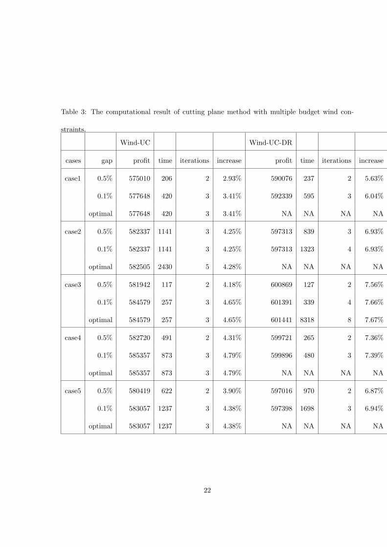
Table 3: The computational result of cutting plane method with multiple budget wind con-
straints.
Wind-UC Wind-UC-DR
cases gap profit time iterations increase profit time iterations increase
case1 0.5% 575010 206 2 2.93% 590076 237 2 5.63%
0.1% 577648 420 3 3.41% 592339 595 3 6.04%
optimal 577648 420 3 3.41% NA NA NA NA
case2 0.5% 582337 1141 3 4.25% 597313 839 3 6.93%
0.1% 582337 1141 3 4.25% 597313 1323 4 6.93%
optimal 582505 2430 5 4.28% NA NA NA NA
case3 0.5% 581942 117 2 4.18% 600869 127 2 7.56%
0.1% 584579 257 3 4.65% 601391 339 4 7.66%
optimal 584579 257 3 4.65% 601441 8318 8 7.67%
case4 0.5% 582720 491 2 4.31% 599721 265 2 7.36%
0.1% 585357 873 3 4.79% 599896 480 3 7.39%
optimal 585357 873 3 4.79% NA NA NA NA
case5 0.5% 580419 622 2 3.90% 597016 970 2 6.87%
0.1% 583057 1237 3 4.38% 597398 1698 3 6.94%
optimal 583057 1237 3 4.38% NA NA NA NA
22

6 Conclusion and Future research
By introducing wind output and demand response, we construct NP-hard two-stage robust
optimization problems and derive mathematical properties of optimal solutions. We develop
a novel cutting plane method to this problem. Our study shows that the robust unit
commitment model with wind and demand response can significantly reduce total operation
cost from thermal units and the novel cutting plane method can dramatically decrease the
computation time compared with traditional Benders decomposition or commercial solvers.
In future (i) more general uncertainty polyhedron will be considered, and (ii) multiple
uncertain factors, such as those from multiple renewable energy sources, will be considered.
References
Elodie Adida and Georgia Perakis. Dynamic pricing and inventory control: Uncertainty
and competition. Operations Research, 58(2):289–302, 2006.
Alper Atamturk and Muhong Zhang. Two-stage robust network flow and design under
demand uncertainty. Operations Research, 55(4):662–673, 2007.
Ross Baldick. The generalized unit commitment problem. Power Systems, IEEE Transac-
tions on, 10(1):465–475, 1995.
Aharon Ben-Tal and Arkadi Nemirovski. Robust convex optimization. Mathematics of
Operations Research, 23(4):769–805, 1998.
Aharon Ben-Tal and Arkadi Nemirovski. Robust solutions of uncertain linear programs.
Operations Research Letters, 25(1):1–14, 1999.
Aharon Ben-Tal and Arkadi Nemirovski. Robust solutions of linear programming problems
contaminated with uncertain data. Mathematical Programming, 88(3):411–424, 2000.
0025-5610.
23
Aharon Ben-Tal and Arkadi Nemirovski. Robust optimization methodology and applica-
tions. Mathematical Programming, 92(3):453–480, 2002. 0025-5610.
Aharon Ben-Tal and Arkadi Nemirovski. Selected topics in robust convex optimization.
Mathematical Programming, 112(1):125–158, 2008.
Dimitris Bertsimas and Melvyn Sim. Robust discrete optimization and network flows. Math-
ematical Programming, 98(1):49–71, 2003. 0025-5610.
Dimitris Bertsimas and Melvyn Sim. The price of robustness. Operations Research, 52(1):
35–53, 2004.
Dimitris Bertsimas and Aurelie Thiele. A robust optimization approach to inventory theory.
Operations Research, 54(1):150–168, 2006.
Daniel Bienstock, George Nemhauser, Dimitris Bertsimas, and Aurlie Thiele. A robust op-
timization approach to supply chain management. In Integer Programming and Com-
binatorial Optimization, Lecture Notes in Computer Science, pages 145–156. Springer
Berlin / Heidelberg, 2004.
Santiago Cerisola, Alvaro Baillo, Jose M. Fernandez-Lopez, Andres Ramos, and Ralf
Gollmer. Stochastic power generation unit commitment in electricity markets: A
novel formulation and a comparison of solution methods. 57(1):32–46, 2009.
Emil M. Constantinescu, Victor M. Zavala, Matthew Rocklin, Sangmin Lee, and Mihai
Anitescu. A computational framework for uncertainty quantification and stochastic
optimization in unit commitment with wind power generation. IEEE transactions on
power systems, accepted.
DoE. 20u.s. electricity supply. Technical report, 2008.
James E. Falk. A linear max-min problem. Mathematical Programming, 5(1):169–188, 1973.
Ahmad Faruqui and Sanem Sergici. Household response to dynamic pricing of electricity-
a survey of experiment evidence. Technical report, 2009.
24

Larry Flowers. Wind powering america update, 2010.
Antonio Frangioni and Claudio Gentile. Solving nonlinear single-unit commitment problems
with ramping constraints. Operations Research, 54(4):767–775, 2006.
Ricardo Fukasawa, Humberto Longo, Jens Lysgaard, Marcus Poggi de Arago, Marcelo Reis,
Eduardo Uchoa, and Renato F. Werneck. Robust branch-and-cut-and-price for the ca-
pacitated vehicle routing problem. Mathematical Programming, 106(3):491–511, 2006.
Laurent El Ghaoui, Maksim Oks, and Francois Oustry. Worst-case value-at-risk and robust
portfolio optimization: A conic programming approach. Operations Research, 51(4):
543–556, 2003.
David Kathan, Caroline Daly, Eric Eversole, Maria Farinella, Jignasa Gadani, Ryan Irwin,
Cory Lankford, Adam Pan, Christina Switzer, and Dean Wright. National action plan
on demand response. Technical report, 2010.
Zhaosong Lu. A computational study on robust portfolio selection based on a joint ellipsoidal
uncertainty set. Mathematical Programming, pages 1–9, 2009.
H. Ma and S. M. Shahidehpour. Unit commitment with transmission security and voltage
constraints. Power Systems, IEEE Transactions on, 14(2):757–764, 1999.
Thomas L. Magnanti and Richard T. Wong. Accelerating benders decomposition: Algorith-
mic enhancement and model selection criteria. Operations Research, 29(3):464–484,
1981.
Bernie Neenan, Donna Pratt, Peter Cappers, James Doane, Jeremey Anderson, Richard
Boisvert, Charles Goldman, Osman Sezgen, Galen Barbose, Ranjit Bharvirkar,
Michael K. Meyer, Steve Shankle, and Derrick Bates. How and why customers re-
spond to electricity price variability: A study of nyiso and nyserda 2002 prl program
performance. Technical report, 2003.
Narayana P. Padhy. Unit commitment-a bibliographical survey. Power Systems, IEEE
Transactions on, 19(2):1196–1205, 2004.
25
Chuen-Teck See and Melvyn Sim. Robust approximation to multiperiod inventory manage-
ment. Operations Research, 58(3):583–594, 2010.
Ramteen Sioshansi and Walter Short. Evaluating the impacts of real-time pricing on the
usage of wind generation. Power Systems, IEEE Transactions on, 24(2):516–524, 2009.
Chua-Liang Su. Optimal Demand-Side Participation in Day-Ahead Electricity Markets.
PhD thesis, University of Mathester, 2007.
Chua-Liang Su and Daniel Kirschen. Quantifying the effect of demand response on electricity
markets. Power Systems, IEEE Transactions on, 24(3):1199–1207, 2009.
A. Takeda, S. Taguchi, and RH Tutuncu. Adjustable robust optimization models for a
nonlinear two-period system. Journal of Optimization Theory and Applications, 136
(2):275–295, 2008. ISSN 0022-3239.
Samer Takriti and Shabbir Ahmed. On robust optimization of two-stage systems. Mathe-
matical Programming, 99(1):109–126, 2004.
Samer Takriti, Benedikt Krasenbrink, and Lilian S. Y. Wu. Incorporating fuel constraints
and electricity spot prices into the stochastic unit commitment problem. 48(2):268–
280, 2000.
Chuang-Li Tseng. On power system generation unit commitment problems. Ph.d., University
of California, Berkeley, 1996.
Aidan Tuohy, Peter Meibom, Eleanor Denny, and Mark O’Malley. Unit commitment for
systems with significant wind penetration. Power Systems, IEEE Transactions on, 24
(2):592–601, 2009.
Jianhui Wang, Audun Botterud, Vladimiro Miranda, Claudio Monteiro, and Gerald Sheble.
Impact of wind power forecasting on unit commitment and dispatch. Technical report,
2009.
Long Zhao and Bo Zeng. An effective cutting plane procedure for two-stage robust opti-
mization problems. Working paper, University of South Florida, 2010.
26