robustness-based design of water distribution networks · robustness-based design of water...

Water Utility Journal 13: 13-28, 2016. © 2016 E.W. Publications

Robustness-based design of water distribution networks

G.D. Puccini*, L.E. Blaser, C.A. Bonetti and A. Butarelli

Universidad Tecnológica Nacional, FRRA, Acuña 49, 2300 Rafaela, Argentina * e-mail: [email protected]

Abstract: Robustness -or lack thereof- is a fundamental property of water distribution systems that has received considerable attention over the last decade. Remarkably, there is still no universally accepted measure of system robustness. Although the resilience index is generally used as a measure of robustness, it is not entirely clear to what extent the resilience captures the network’s ability to operate under pipe bursts. This paper presents a measure of system robustness that quantifies the capability of a water distribution network to maintain its function under perturbations in structure. This new index, called robustness, is used for the multi-objective design of two widely studied water distribution networks. It is also applied to a real network with a strong topological weakness that, in case of a localized failure, may impact dramatically on the rest of the system. It is found that robustness-based designs display a better performance to pipe bursts than those based on the resilience index.

Key words: multi-objective, network design, optimization, resilience, robustness, water supply

1. INTRODUCTION

A water distribution system consists of pipes, pumps, valves, tanks and reservoirs to deliver water to consumers at required minimum pressures. The design of these water systems is a process that typically consists in determining the optimal components for a given network topology. In the past, optimization techniques were limited to the case of single-objective optimization (Alperovits and Shamir, 1977; Lansey and Mays, 1989; Eiger et al., 1994; Savic and Walters, 1997; Geem, 2006). They were mainly oriented to find the combination of commercial pipes (and, eventually, also pumps and tanks) that minimizes the network cost while maintaining a set of hydraulic constraints such as demand and minimum pressure head at each node. In most cases, optimization was studied in two different ways: by reducing pipe diameters or removing pipes in loops. Unfortunately, the solution obtained from any of these ways is not completely satisfactory because it makes the network operational, but it does not ensure an adequate supply of water to consumers under abnormal conditions. Undesirable events occur in every water distribution system, either by failures of mechanical components (pipes, valves, or pumps) or by fluctuations on demands (Farmani et al., 2005). This creates an uncertain situation since the system may not be able to meet the designed demands or the required pressure heads.

In the last two decades, the reliability of water distribution systems has received considerable attention. The need for new optimization strategies addressing the design not only with minimal cost but also with maximal benefits through a reliability assessment was stressed by Walski (2001). The term “reliability” does not have a clearly defined meaning (see Ostfeld (2004) for a complete overview up to 2002). Nevertheless, it is generally understood that reliability is concerned with the ability of a system to provide an adequate supply to consumers, under both normal and abnormal operating conditions (Goulter, 1995). Reliability is often treated as a stochastic variable accounting not only for the probability of failure of mechanical components of the network (Su et al., 1987; Xu and Goulter, 1999; Fujiwara and Silva, 1990; Cullinane et al., 1992; Tanyimboh and Templeman, 2000; Martinez-Rodríguez et al., 2011), but also other sources of uncertainty of network operating conditions (Lansey et al., 1989; Xu and Goulter, 1999; Gargano and Pianese, 2000; Babayan, 2005; Surendran et al., 2005). The reliability-based design of a water distribution system requires the knowledge of the probabilities of undesirable events, such as failures of the system components,

14 G.D. Puccini et al.

and the impact of these events on the consumer demands. However, these probabilities are generally not known, which makes any estimation of reliability difficult and questionable.

The term “robustness" has also been considered in water distribution systems (Kapelan et al., 2005; Jung et al., 2014; Greco et al., 2012). Robustness is generally thought of as reflecting the ability of a system to withstand perturbations in structure without changes in function (Jen, 2003). Unlike reliability, robustness is usually treated as a deterministic concept (Greco et al., 2012) addressed to avoid or minimize the failure severity rather than to focus on the probability of a successful operation (Jung et al., 2014). Conceptually close to the above definition of network robustness is the “resilience” index introduced by Todini (2000), and defined as the ability of a system to overcome critical operating conditions. The resilience index is characterized by a surplus head at each node, in such a way that this excess of head is available to be dissipated internally in case of failures (Todini, 2000; Prasad and Park, 2004; Jayaram and Srinivasan, 2008). This definition was motivated by the fact that, under abnormal conditions, the original network will become a new one with higher internal energy losses. Thus, increasing resilience means providing more power than required at each node to overcome the higher internal losses. Therefore, an increase in the resilience index should be accompanied by an increase of system robustness. Several authors have used and tested the resilience index for multi-objective optimal design procedures (Farmani et al., 2006; Saldarriaga et al., 2010; Vasan and Simonovic, 2010; Baños et al., 2011). Also, the resilience index has been used as an indirect method for assessing the performance of a system (Tsakiris and Spiliotis, 2012). Another study investigates the potential use of resilience and network entropy as indexes of network robustness (Greco et al., 2012; see also Herrera at al., 2016). Although these authors show that resilience is better than entropy to quantify system robustness, it is not entirely clear to what extent the resilience index allows for measuring the network capability to operate under mechanical failures.

This paper presents an index, called robustness, that explicitly considers the capability of a water distribution system to maintain its function under a perturbation in structure. The proposed index basically measures the number of nodes with insufficient pressure head as a consequence of the failure of one pipe. Thus, the robustness-based design seeks to minimize the failure severity by minimizing the number of nodes with pressure deficits. This is achieved during the optimization process by monitoring the network performance under each system perturbation. The main aim of this study is to compare two possible quantifications of network robustness (with regards to mechanical failures): the resilience index of Todini (2000), and the robustness index proposed here. To test the usefulness for evaluating the network robustness of both indexes, three examples are investigated. The first two examples are widely known academic problems and the last one is a real network that is largely vulnerable to mechanical pipe failures. Simulated annealing is used to solve the multi-objective optimization problems and post-optimization analyses are performed to analyze the resulting designs.

2. METHODS

2.1 Hydraulic model

Hydraulic relationships in a water distribution system are given by conservation of mass and energy. Mass conservation must be satisfied at each node and can be written:

𝑄!!!!

i=! =q! , 𝑗 = 1,⋯ ,𝑁! nodes (1)

where 𝑄!! is the flow in pipe i connected to node j, 𝑁! is the number of pipes connected to node j,

and 𝑞! is the demand at node j. Energy conservation states that the sum of the head losses, Δh, around each closed loop l must be zero:

Water Utility Journal 13 (2016) 15

Δℎ!!!∈! = 0, 𝑙 = 1,⋯ ,𝑁! loops (2)

Moreover, the head ℎ! at each node j must satisfy a given minimum pressure head ℎ!∗ requirement:

ℎ! ≥ ℎ!∗, 𝑗 = 1,⋯ ,𝑁! nodes (3)

The Hazen-Williams equation Δℎ =α𝐿𝐷!!.87 𝑄 𝐶 !.852 is widely used to estimate the head loss Δℎ in pipes, where 𝛼 is a numerical conversion constant whose numerical value depends on the used units, 𝐿 is the length of the pipe, 𝑄 is the flow rate and 𝐶 is a Hazen-Williams roughness coefficient of the pipe. Moreover, all heads at tanks and reservoirs must be specified as boundary conditions. Here, the EPANET software (Rossman, 2000) is used, which iteratively solves this set of nonlinear equations using the gradient method proposed by Todini and Pilati (1987). Recently, a different model based on a heuristic optimization procedure was proposed by Spiliotis (2014). It should be noted that EPANET is a software based on the assumption of fixed demands, i.e. demand-driven approach (DDA), which is unable to predict the actual nodal demands in conditions of pressure deficit. A more realistic modeling of the hydraulic system is based on a pressure-driven approach (PDA) in which demands are assumed to be driven by pressure, i.e. 𝑞!= 𝑓(ℎ!) at each node j (see Gupta and Bhave (1996); Kalungi and Tanyimboh (2003); Todini (2003); Giustolisi et al. (2008); Tsakiris and Spiliotis (2014) for different models of pressure-driven demand). Both strategies, DDA and PDA, are allowed in optimization problems, but the decision influences the computational burden. The use of PDA for optimal design provides a more realistic picture of the system than DDA, but is computationally more expensive due to the increased complexity of the model (Giustolisi et al., 2014).

2.2 Multi-objective problem

In multi-objective optimization, typically there is no single optimal solution, but a set of solutions, called Pareto optimal set, which are all considered to be equally important (Hans, 1988). To define the Pareto set in the context of a minimization problem for the objective functions 𝑓!,… ,𝑓! with 𝑁 ≥ 2, any two feasible solutions 𝑥! and 𝑥! have to be compared with the aim of

finding the set of solutions that cannot be improved in any of the objectives without degrading at least one of the other objectives. Formally, the solution 𝑥! is said to dominate 𝑥! if both the following conditions are true:

(a) 𝑥! is better than 𝑥! in at least one objective: ∃𝑖 𝑖=1,2,… ,N , 𝑓! 𝑥! < 𝑓! 𝑥! . (b) 𝑥! is not worse in all objectives: ∀𝑖 𝑖=1,2,… ,N , 𝑓! 𝑥! ≤ 𝑓! 𝑥! . If 𝑥! dominates the solution 𝑥! then 𝑥! is said to be a nondominated solution. The set of

nondominated solutions is known as the Pareto optimal set. Once the Pareto set is determined, it usually requires several considerations in order to choose the solution to be implemented. The multi-objective problem for the robustness-based design presented here is stated as: (1) minimize the network cost, and (2) maximize the network robustness. More specifically, the problem is formulated as follows:

Minimize 𝑓! = 𝐶!!!=! 𝐷!, L! (4)

Maximize 𝑓!=I! (5)

where 𝐶 𝐷! , L! denotes the cost of the pipe i with diameter 𝐷! and length 𝐿!, 𝑁! denotes the number of pipes of the system and 𝐼! denotes the index to be investigated, either the resilience 𝐼res or the robustness index 𝐼!.


2.3 Robustness measures and unfeasible solutions

In this paper, two measures of network robustness are used to obtain different Pareto fronts: (1) resilience index and (2) robustness index.

2.3.1 Resilience index

The resilience index 𝐼res was defined by Todini (2000) as:

𝐼res = 1 − !!"#∗

!!"#∗ (6)

where 𝑃!"#∗ =𝛾 𝑄!!!!=! 𝐻! − 𝛾 𝑞!∗

!!!=! ℎ! is the amount of power dissipated in the network to satisfy

the total demand, and 𝑃!"#∗ =𝛾 𝑄!!!!=! 𝐻! − 𝛾 𝑞!∗

!!!=! ℎ!∗ is the maximum power that would be

dissipated internally in order to satisfy the constraints in terms of demand 𝑞!∗ and head ℎ!∗ at node i. Moreover, 𝑁! is the number of demand nodes, 𝑄! and 𝐻! are the discharge and the head, respectively, to each reservoir k, with 𝑁! being the number of reservoirs and γ the specific weight of water. After substitution of these quantities, the resilience index can be written as:

𝐼res =!!∗!!

!=! (!!!!!∗)

!!!!!=! !!! !!

∗!!!=! !!

∗ (7)

Some authors have extended the resilience index (Prasad and Park, 2004; Jayaram and Srinivasan, 2008) in order to overcome certain minor drawbacks. A complete study that compares the performance of these resilience indexes is given by Baños et al. (2011). This paper compares the original resilience index proposed by Todini (2000) with the robustness index defined below.

2.3.2 Robustness index

In general terms, robustness is usually thought of as reflecting the ability of a system to withstand a perturbation in structure without change in function (Jen, 2003). By following this idea, a robustness index is introduced here to account for the ability of a water distribution system to maintain its function despite perturbations in structure. Therefore, the network capability to operate under the failure of a single pipe must be mathematically characterized. Let 𝑁!out 𝑁! be the fraction of nodes with pressure deficits (i.e. nodes with pressure below the minimum pressure head) due to the failure of pipe number k, where 𝑁! is the number of demand nodes. This number describes the weakness of the network under the failure of pipe number k. In order to characterize the overall response of the network, the sum over all failure possibilities, that is, on all pipes must be considered:

𝑁! = !!!

!!out

!!+ !!out

!!+⋯+

!!!out

!!=

!!out!!

!=!!!!!

(8)

where it has been divided by the total number of pipes 𝑁! to allow for the comparison of networks with different dimensions. Thus, 𝑁! measures the weakness of a given network configuration under the failure of any pipe. The robustness index is defined as: 𝐼! = 1− 𝑁!. For instance, a network composed of two loops as the one given in Section 3 (see Fig. 1a) with 𝑁! = 6 (consumers) and 𝑁! = 8 achieves the maximal value of the robustness index 𝐼! = 0.875 when 𝑁!out = 0 for all 𝑘 ≠ 1 and 𝑁!out = 6: the failure of pipe number 1 (which connects the reservoir 𝑁1 with the rest of the network) affects all nodes, and the failure of any other pipe does not produce damage. On the


other hand, a network design achieves the minimal value of the robustness index 𝐼! = 0 when 𝑁!out = 6 for all k: each removed pipe causes the maximal fraction of nodes with pressure deficits.

2.3.3 Unfeasible solutions during optimization process

Both measures of network robustness are positive quantities for any feasible solution. However, the resilience index achieves negative values for those solutions with pressure deficits. Although such a problem has no place for the robustness index because it directly counts the number of nodes (and, therefore, it is positive), it is also necessary to give a special treatment to those candidate solutions that, under normal operating conditions, do not satisfy the requirement of minimum pressure. To identify and evaluate the depth of failure of unfeasible solutions appearing during the optimization process, it is useful to consider a penalty function. In the context of a minimization problem (i.e. 𝑓! = 1− 𝐼!), a penalty function 𝑃! is used to increase the values of the objective functions for those solutions with nodal pressures ℎ! lower than the minimum pressure head ℎ!∗:

𝑃!=K (ℎ!∗ − ℎ!)!!!=! , ∀𝑗: ℎ! < ℎ!∗ (9)

where the sum runs for all nodal pressures which do not satisfy the minimum pressure head requirement. In order to compare properly, the same penalty function is used for both indexes with K = 1.0×10! for 𝑓! (cost function) and K = 10 for 𝑓!. The values for 𝐾 were found by a trial-and-error procedure according to the sensitivity of the optimization process to the different units of each objective function.

2.4 Simulated annealing for multi-objective optimization

Several algorithms have been developed for dealing with both single- and multi-objective optimization problems. Evolutionary algorithms are one of these algorithms that have become very popular in the last decade (Prasad et al., 2003; Kapelan et al., 2005; Suribabu and Neelakantan, 2006; Wang et al., 2014; Mora-Melia et al., 2015). Simulated annealing is another well known algorithm which has also been extended for dealing with multi-objective problems. Originally developed for single objective optimization problems (Kirkpatrick et al., 1983), simulated annealing is based on a generalization of the strategy of iterative progress, which starts with an initial solution and then it searches, within its environment, another lower-cost solution. The generalization introduced by simulated annealing involves the acceptance, with a non-zero probability, of a higher-cost solution to avoid getting trapped in a local minimum.

The multi-objective version presents a number of advantages when compared with other methods: (a) it is simple, (b) it can find multiple solutions in a single run, and (c) it converges rapidly to the Pareto set. A review of different implementations of the simulated annealing algorithm for multi-objective problems can be found in Suman and Kumar (2006). Here, the method of Suppapitnarm et al. (2000) is implemented, which can be summarized as follow:

1. An initial set of nondominated solutions is randomly generated. 2. A new solution y is generated by perturbation of a solution x randomly selected from the

initial nondominated set. The objective functions are evaluated and, if necessary, a penalty function is applied.

3. If the new solution is better than the current solution in at least one objective, the Pareto set is updated and the new solution is made the current solution.

4. If the new solution is not accepted in the previous step, it can be accepted according to the products of the Boltzmann probabilities of each objective:


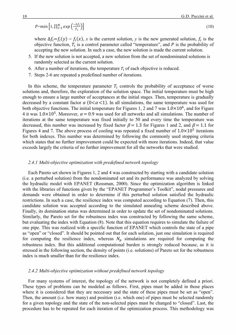
𝑃=𝑚𝑖𝑛 1, 𝑒𝑥𝑝!!=!

!Δ!!!!

(10)

where Δ𝑓!=𝑓! 𝑦 − 𝑓! 𝑥 , x is the current solution, y is the new generated solution, 𝑓! is the objective function, 𝑇! is a control parameter called “temperature”, and 𝑃 is the probability of accepting the new solution. In such a case, the new solution is made the current solution.

5. If the new solution is not accepted, a new solution from the set of nondominated solutions is randomly selected as the current solution.

6. After a number of iterations, the temperature 𝑇! of each objective is reduced. 7. Steps 2-6 are repeated a predefined number of iterations. In this scheme, the temperature parameter 𝑇! controls the probability of acceptance of worse

solutions and, therefore, the exploration of the solution space. The initial temperature must be high enough to ensure a large number of acceptances at the initial stages. Then, temperature is gradually decreased by a constant factor 𝛼 0<α <1 . In all simulations, the same temperature was used for both objective functions. The initial temperature for Figures 1, 2 and 7 was 1.0×10!, and for Figure 4 it was 1.0×10!. Moreover, α = 0.9 was used for all networks and all simulations. The number of iterations at the same temperature was fixed initially to 50 and every time the temperature was decreased, this number was increased by fixed factor β = 1.3 for Figures 1 and 2, and β = 1.1 for Figures 4 and 7. The above process of cooling was repeated a fixed number of 1.0×10! iterations for both indexes. This number was determined by following the commonly used stopping criteria which states that no further improvement could be expected with more iterations. Indeed, that value exceeds largely the criteria of no further improvement for all the networks that were studied.

2.4.1 Multi-objective optimization with predefined network topology

Each Pareto set shown in Figures 1, 2 and 4 was constructed by starting with a candidate solution (i.e. a perturbed solution) from the nondominated set and its performance was analyzed by solving the hydraulic model with EPANET (Rossman, 2000). Since the optimization algorithm is linked with the libraries of functions given by the “EPANET Programmer’s Toolkit”, nodal pressures and demands were obtained in order to determine if this perturbed solution satisfied the hydraulic restrictions. In such a case, the resilience index was computed according to Equation (7). Then, this candidate solution was accepted according to the simulated annealing scheme described above. Finally, its domination status was determined in order to update the set of nondominated solutions. Similarly, the Pareto set for the robustness index was constructed by following the same scheme, but evaluating the index with Equation (8). Note that this equation requires to simulate the failure of one pipe. This was realized with a specific function of EPANET which controls the state of a pipe as “open” or “closed”. It should be pointed out that for each solution, just one simulation is required for computing the resilience index, whereas 𝑁! simulations are required for computing the robustness index. But this additional computational burden is strongly reduced because, as it is stressed in the following section, the density of points (i.e. solutions) of Pareto set for the robustness index is much smaller than for the resilience index.

2.4.2 Multi-objective optimization without predefined network topology

For many systems of interest, the topology of the network is not completely defined a priori. These types of problems can be modeled as follows. First, pipes must be added in those places where it is considered that they are necessary and the state of these pipes must be set as “open”. Then, the amount (i.e. how many) and position (i.e. which one) of pipes must be selected randomly for a given topology and the state of the non-selected pipes must be changed to “closed”. Last, the procedure has to be repeated for each iteration of the optimization process. This methodology was


applied to the system shown in Figure 6. For each Pareto set in Figure 7, the upper and lower part of the city were connected by adding nine pipes (of higher diameter) between the closest nodes. Then, a topology was randomly chosen by closing a set of pipes between the two parts of the city. As an additional restriction, the connection cost of any of these nine pipes is more expensive than the cost of placing pipes on the rest of the network: it is estimated to be equivalent to increasing the costs of each pipe by four. This fact was modeled as a penalty factor that affects only the pipes at this zone. The performance of each candidate solution (i.e. topology and set of diameters) was evaluated with EPANET and each index was computed as described above.

2.5 Post-optimization analyses

All the analyses shown in Figures 2, 3, 4 and 7 were conducted on solutions of each Pareto set. A separate code searched the solutions on each set having the minimal (absolute) difference in cost. For instance, the mean value of the difference in cost between two solutions belonging to each Pareto set in Figure 2 is 1.2x103 and the standard deviation 0.7x103 is (cost units). The results do not depend critically on this difference. Moreover, all hydraulic parameters required for the analyses of those figures were obtained by using the libraries of functions given by the “EPANET Programmer’s Toolkit”.

3. SAMPLE APPLICATIONS

The suitability of the two measures of network robustness is evaluated by studying three sample applications.

3.1 Two-loop network

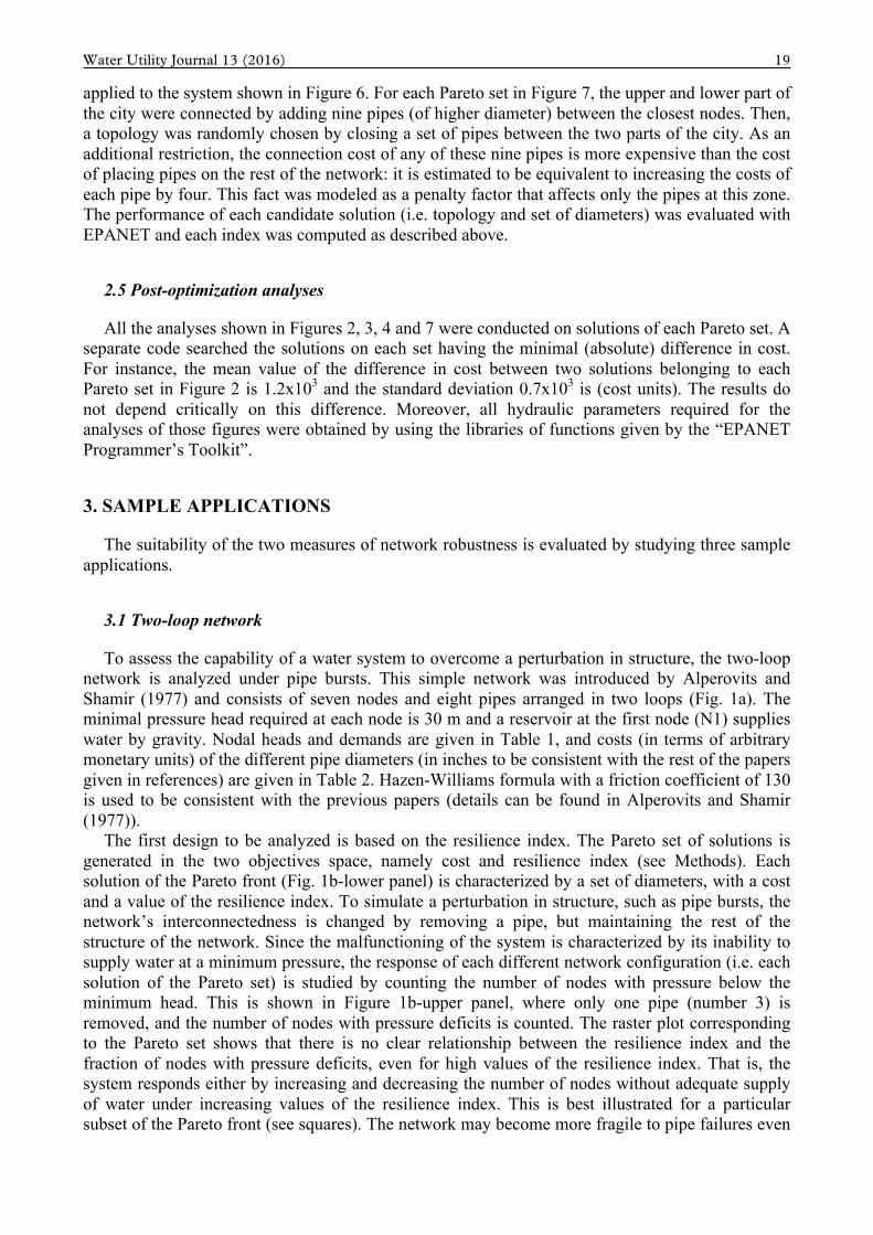
To assess the capability of a water system to overcome a perturbation in structure, the two-loop network is analyzed under pipe bursts. This simple network was introduced by Alperovits and Shamir (1977) and consists of seven nodes and eight pipes arranged in two loops (Fig. 1a). The minimal pressure head required at each node is 30 m and a reservoir at the first node (N1) supplies water by gravity. Nodal heads and demands are given in Table 1, and costs (in terms of arbitrary monetary units) of the different pipe diameters (in inches to be consistent with the rest of the papers given in references) are given in Table 2. Hazen-Williams formula with a friction coefficient of 130 is used to be consistent with the previous papers (details can be found in Alperovits and Shamir (1977)).

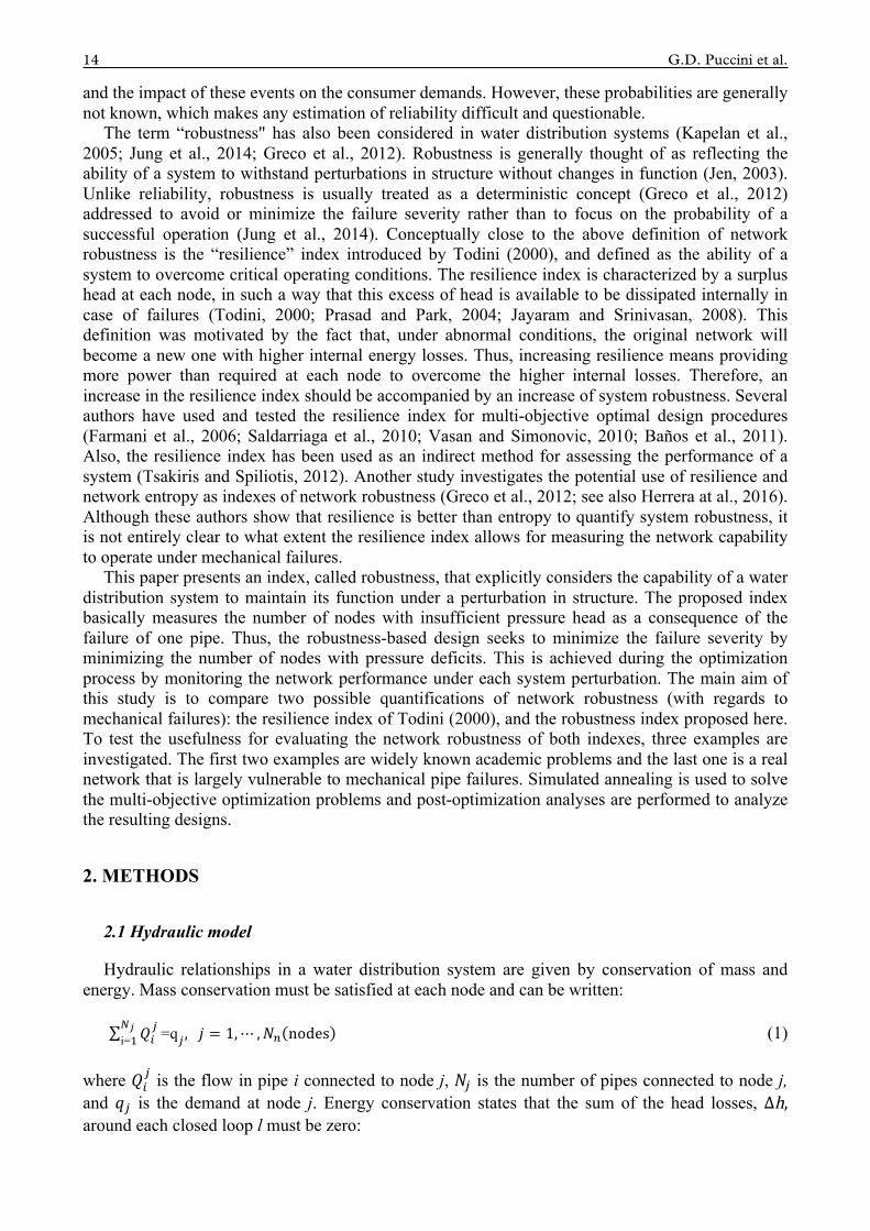
The first design to be analyzed is based on the resilience index. The Pareto set of solutions is generated in the two objectives space, namely cost and resilience index (see Methods). Each solution of the Pareto front (Fig. 1b-lower panel) is characterized by a set of diameters, with a cost and a value of the resilience index. To simulate a perturbation in structure, such as pipe bursts, the network’s interconnectedness is changed by removing a pipe, but maintaining the rest of the structure of the network. Since the malfunctioning of the system is characterized by its inability to supply water at a minimum pressure, the response of each different network configuration (i.e. each solution of the Pareto set) is studied by counting the number of nodes with pressure below the minimum head. This is shown in Figure 1b-upper panel, where only one pipe (number 3) is removed, and the number of nodes with pressure deficits is counted. The raster plot corresponding to the Pareto set shows that there is no clear relationship between the resilience index and the fraction of nodes with pressure deficits, even for high values of the resilience index. That is, the system responds either by increasing and decreasing the number of nodes without adequate supply of water under increasing values of the resilience index. This is best illustrated for a particular subset of the Pareto front (see squares). The network may become more fragile to pipe failures even


for increasing values of the resilience index. In other words, a more expensive system could be more vulnerable to mechanical pipe failures. Although these responses are caused by the failure of a particular pipe, the elimination of different pipes produces approximately the same behavior: removing pipe 1 produces maximal damage (for all configurations) because no node is served, whereas removing pipe 4 produces minimal damage (for most configurations).

Table 1: Head and demand values for the two-loop network.

Node Head (m) Demand (m3/h) 1 210 -1120 2 150 100 3 160 100 4 155 120 5 150 270 6 165 330 7 160 200

Table 2: Diameters and cost of pipes for the two-loop network

Diameters (inches)

Cost (units)

1 2

2 5 3 8 4 11 6 16 8 23

10 32 12 50 14 60 16 90 18 130 20 170 22 300 24 550

Figure 1: (a) Two-loop network. Numbers identify nodes and pipes (reservoir at N1). (b) Lower panel, Pareto set (dots) and particular solutions (squares). Upper panel, fraction of nodes with pressure deficits corresponding to the solutions

showed in the lower panel.

Next, the robustness index is used to obtain a new Pareto front for two-loop network (see Methods). It should be noted that maximizing the robustness index is equivalent to minimizing the fraction of nodes with pressure below the minimal pressure head. Figure 2a shows the Pareto front so obtained (squares) and that obtained by using the resilience index (circles). Inset shows the


complete Pareto sets. A rather different feature is observed: the robustness index produces a Pareto front with lower density of points. This occurs because the minimum step between any two solutions is given by Δ𝐼! = 1 𝑁! 𝑁!. Note, however, that the number of solutions will increase with the size of the network, giving a higher density of points for larger networks. In addition, note that no conclusion should be made about the degree of system robustness of the two kinds of solutions because the two Pareto sets were obtained under different indexes.

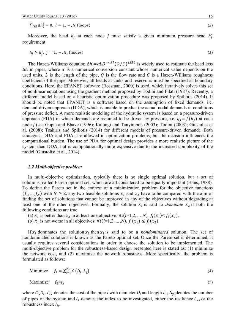
In order to compare the two indexes properly, the study must be restricted to a subset of each Pareto front with solutions having (approximately) the same cost (see Methods). The response of the system is represented as the percentage of nodes with pressure deficits (Fig. 2b). It is observed that the solutions obtained with the robustness index are much less vulnerable to pipe failures than those obtained with the resilience index. Moreover, when both kinds of solutions are considered globally, the malfunctioning of the network decreases with increasing cost. However, this behavior is rather different for neighboring points: the fraction of nodes with pressure deficits decreases monotonically with cost only for the robustness index. This negative correlation is an important feature of the index proposed in this paper: it provides an unambiguous guide for the designer because a more expensive pipe arrangement necessarily means a more robust network under pipe bursts.

The removal of a pipe alters the network topology and, as a consequence, velocities increase in some pipes and so do the hydraulic losses. Despite the fact that the resilience index is characterized by a surplus head at each node which is available to be dissipated internally in case of failures, the above finding shows that an increase of resilience index is not necessarily accompanied by an increase of system robustness.

Figure 2: Comparative responses of the two-loop network under the failure of one pipe. (a) Pareto fronts for both network robustness measures (i.e. resilience and robustness index). Inset shows the complete Pareto set. (b-c)

Responses for the same cost solutions of the Pareto set.

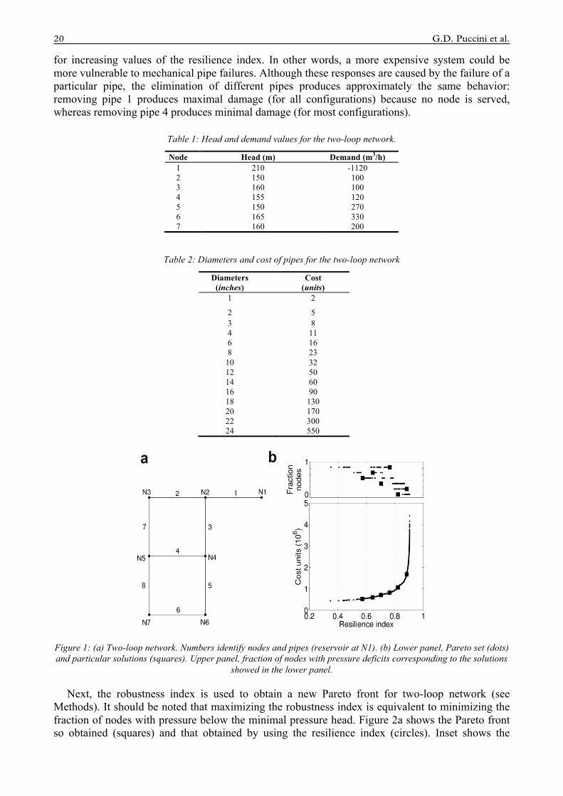
In contrast, the proposed robustness index displays solutions with high degree of tolerance against pipe bursts. To better understand this result, the flow distribution is analyzed after a perturbation in structure. This is obtained by counting the number of pipes with velocities larger than 2 m/s as a consequence of removing a pipe. The process is repeated for all pipes and the result is finally averaged (Fig. 2c). It is found that, under these extreme conditions, the network shows high velocities for both indexes, but the solutions obtained with the robustness index display the best behavior. Indeed, tolerance to pipe failures comes at the expense of high velocities in other pipes. But velocities larger than 2 m/s in an increasing number of pipes cause increasing hydraulic losses, making the flow distribution between nodes highly inefficient. Table 3 shows pipe diameters for each solution of Figure 2b-c obtained with the resilience index. It is observed that the resilience-based design assigns small diameters to pipes 4 and 6, giving more weight to ‘vertical’ pipes (i.e. 3, 5, 7 and 8).


Table 3: Pipe diameters (inches) of resilience-based solutions for the two-loop network.

Pipe S1 S2 S3 S4 S5 S6 S7 S8 S9 S10 S11 S12 S13 S14 S15 S16 S17 S18 1 18 20 20 20 20 20 20 20 20 20 20 20 20 20 20 22 22 22 2 14 14 14 14 14 16 16 16 16 16 16 18 16 14 16 16 14 16 3 14 14 14 14 14 14 14 14 16 16 16 16 18 20 20 18 20 20 4 2 3 1 3 3 2 2 6 1 2 2 1 14 14 14 14 14 14 5 14 12 14 14 14 14 14 14 14 14 14 14 14 16 16 14 16 16 6 1 1 1 1 1 2 1 1 4 1 1 1 2 4 2 1 1 4 7 14 14 14 14 14 14 14 14 14 16 16 16 14 14 12 14 12 16 8 14 10 10 10 12 10 12 12 10 10 12 12 14 14 14 12 14 14

Table 4: Pipe diameters (inches) of robustness-based solutions for the two-loop network.

Pipe S1 S2 S3 S4 S5 S6 S7 S8 S9 S10 S11 S12 S13 S14 S15 S16 S17 S18

1 20 18 18 18 20 18 20 20 20 20 20 20 20 20 20 20 20 20 2 12 8 8 10 10 10 10 10 10 10 10 12 16 16 16 16 18 18 3 16 18 18 18 18 18 18 18 18 18 18 18 18 18 18 18 18 18 4 1 10 10 10 10 14 12 12 12 12 12 14 14 12 14 14 14 14 5 14 16 16 16 14 16 14 14 14 14 14 14 14 14 14 14 14 14 6 10 10 10 10 10 10 10 10 10 10 10 10 10 10 10 14 14 14 7 10 1 2 2 4 2 6 10 10 10 12 10 10 16 16 16 16 20 8 1 1 1 1 1 1 3 1 3 10 10 14 14 14 14 16 16 16

In that approach, pipes 4 and 6 are considered as redundant, with the main function of close

loops, but without the capability to overcome the increased flow produced by the failure of any other pipe. In addition, note that the better performance of solution 13 (Fig. 2b-c), compared with solution 12, can mainly be explained by the increased diameter of pipe 4 (compare S12 with S13 in Table 3). Thus, despite the surplus head provided by the resilience-based design, the supply of water between nodes is increasingly difficult when the remaining pipes do not have the sufficient capability (i.e. diameter) to handle the increased flow. This finding is consistent with that obtained by Greco et al. (2012), by Martinez-Rodríguez et al. (2011) and also by Herrera et al. (2016), asserting that entropy, being a measure of topological redundancy, by itself does not ensure system robustness. On the other hand, the robustness-based design displays better ability than the resilience-based design to overcome pipe bursts because it is able to distribute the flow more efficiently on the unaffected part of the network. This behavior is consistent with the scenario observed in Table 4: the robustness-based design does not give minor importance to pipes 4 and 6 than to any other pipe. The only exception is solution 1 (S1), with 1-in-diameter in pipe 4, which displays a high number of pipes with velocity larger than 2 m/s (Fig. 2c).

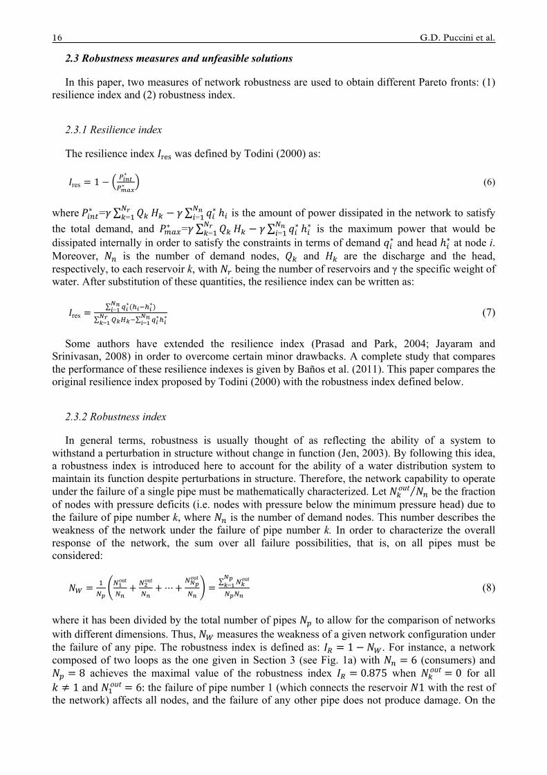
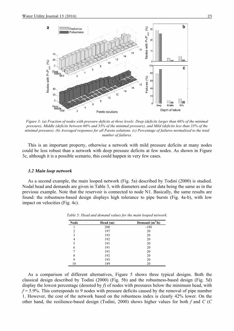
The depth of pressure deficits is another critical factor to be considered for robustness. To better understand the impact of pipe bursts to the extent of pressure deficits, the number of failures for each Pareto solution is analyzed by counting the number of nodes with pressure deficits 𝐷= ℎ − ℎ* ℎ* at three different levels (Fig. 3a): deep deficits (𝐷 >66%), middle deficits (33%< 𝐷 <66%) and mild deficits (𝐷 < 33%). The response of the resilience and the robustness index is similar for all solutions: the fraction of nodes with deep deficits dominates both mild and middle deficits. However, the robustness-based design shows a more clear decreasing behavior of deep failures for increasing cost. The percentage of nodes with mild and middle deficits is maintained approximately at the same low values for all solutions. Thus, the robustness index provides the smallest averaged responses for all Pareto solutions (Fig. 3b) at the three deficit levels. It is also important to consider the number of failures at each deficit level normalized to the total number of failures (Fig. 3c). The percentage of deep deficits for the robustness index achieves a value of 90% whereas middle and mild deficits are close to 5% each. Therefore, the majority of pressure deficits is dominated by deep failures, and nodes with mild deficits appear rarely.


Figure 3: (a) Fraction of nodes with pressure deficits at three levels: Deep (deficits larger than 66% of the minimal pressure), Middle (deficits between 66% and 33% of the minimal pressure), and Mild (deficits less than 33% of the

minimal pressure). (b) Averaged responses for all Pareto solutions. (c) Percentage of failures normalized to the total number of failures.

This is an important property, otherwise a network with mild pressure deficits at many nodes could be less robust than a network with deep pressure deficits at few nodes. As shown in Figure 3c, although it is a possible scenario, this could happen in very few cases.

3.2 Main loop network

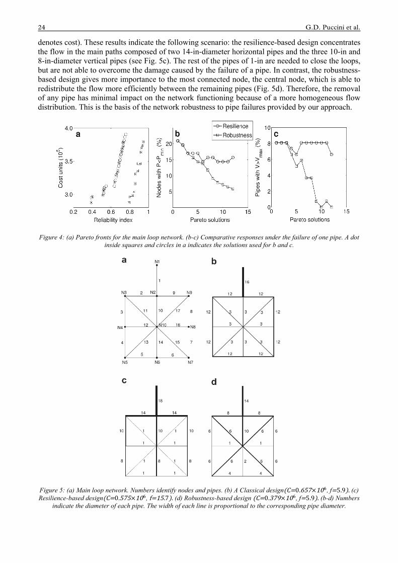
As a second example, the main looped network (Fig. 5a) described by Todini (2000) is studied. Nodal head and demands are given in Table 3, with diameters and cost data being the same as in the previous example. Note that the reservoir is connected to node N1. Basically, the same results are found: the robustness-based design displays high tolerance to pipe bursts (Fig. 4a-b), with low impact on velocities (Fig. 4c).

Table 5: Head and demand values for the main looped network.

Node Head (m) Demand (m3/h) 1 200 -180 2 197 20 3 193 20 4 192 20 5 191 20 6 191 20 7 8 9

10

191 192 193 189

20 20 20 20

As a comparison of different alternatives, Figure 5 shows three typical designs. Both the

classical design described by Todini (2000) (Fig. 5b) and the robustness-based design (Fig. 5d) display the lowest percentage (denoted by f) of nodes with pressures below the minimum head, with f = 5.9%. This corresponds to 9 nodes with pressure deficits caused by the removal of pipe number 1. However, the cost of the network based on the robustness index is clearly 42% lower. On the other hand, the resilience-based design (Todini, 2000) shows higher values for both f and C (C


denotes cost). These results indicate the following scenario: the resilience-based design concentrates the flow in the main paths composed of two 14-in-diameter horizontal pipes and the three 10-in and 8-in-diameter vertical pipes (see Fig. 5c). The rest of the pipes of 1-in are needed to close the loops, but are not able to overcome the damage caused by the failure of a pipe. In contrast, the robustness-based design gives more importance to the most connected node, the central node, which is able to redistribute the flow more efficiently between the remaining pipes (Fig. 5d). Therefore, the removal of any pipe has minimal impact on the network functioning because of a more homogeneous flow distribution. This is the basis of the network robustness to pipe failures provided by our approach.

Figure 4: (a) Pareto fronts for the main loop network. (b-c) Comparative responses under the failure of one pipe. A dot inside squares and circles in a indicates the solutions used for b and c.

Figure 5: (a) Main loop network. Numbers identify nodes and pipes. (b) A Classical design(C=0.657×10!, f=5.9). (c) Resilience-based design(C=0.575×10!, f=15.7). (d) Robustness-based design (C=0.379×10!, f=5.9). (b-d) Numbers

indicate the diameter of each pipe. The width of each line is proportional to the corresponding pipe diameter.


3.3 A real application: La Para network

Some real networks are characterized by a dramatic vulnerability to pipe failures. The proposed methodology may be useful for those seeking a robust design. As an illustrative example, the La Para water distribution system, in Argentina, is studied (see Fig. 6). This system is composed by two networks which are separated by the train rails. The zone between the two parts of the city is called “critical zone”. The lower and the upper parts are composed of 59 and 78 nodes respectively, with a mean nodal demand of 0.54 m3/h. A tank, at the lower part of the network, delivers water to the two systems which are connected by a single pipe of 151 mm. This pipe, however, is inadequate to meet the minimal pressure and demand requirements for all the consumers in the upper network. Moreover, this configuration is extremely vulnerable since any failure on this pipe alters dramatically the network connectivity: the upper part of the city breaks apart, forming a system without any water service. Here the problem consists in finding the commercial pipe diameters for the complete system, including the connection between the two networks. Therefore, the optimization process is oriented to determine the pipe diameters for both networks and, moreover, the amount, location and diameters of the pipes that connect them (see Methods).

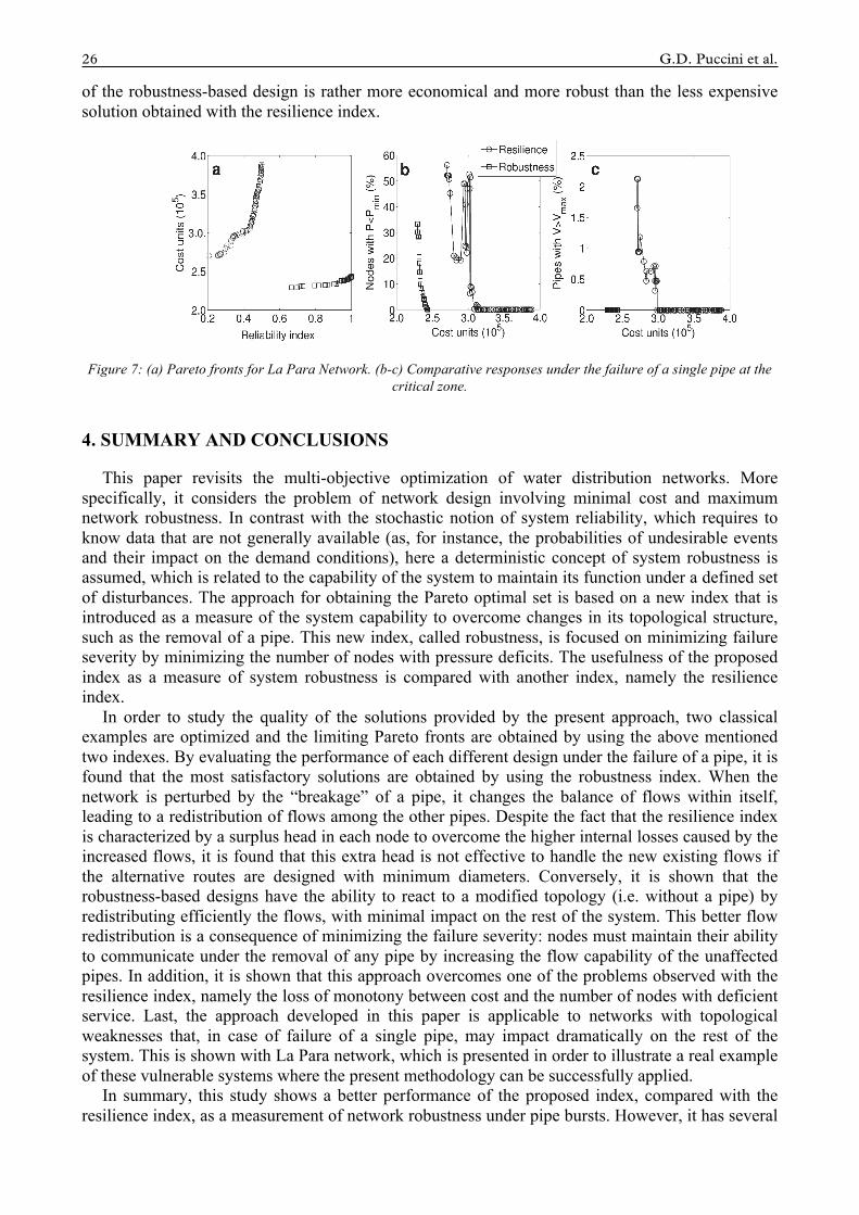
Pareto fronts for each index are shown in Figure 7a. This example displays a rather different feature: all solutions resulting from the use of the robustness index are less expensive than those obtained with the resilience index. To investigate the degree of network robustness under pipe bursts, the number of nodes with deficient service (i.e. pressure below the minimal head) is counted when each pipe belonging to the critical zone is removed. In addition, the number of pipes in which the velocity is larger than 2 m/s is counted.

Figure 6: La Para network. Thick lines indicate the location of new pipes for the lowest cost solution of the robustness-based design.

This is repeated for all solutions of each Pareto front. Because the two Pareto fronts have no solutions with equal cost, in Figure 7b-c the fraction of nodes with pressure deficits and the fraction of pipes with velocity larger than 2 m/s are plotted versus cost units. Note that for all solutions obtained with the robustness index, there is no pipe in which the velocity is larger than 2 m/s. In addition, it should be observed that the solutions based on the robustness index are less expensive ( ≃ 0.5×10!) for the same degree of network robustness. As an illustrative example, Figure 6 (thick lines) represents the four new pipes of diameters 𝐷= 59, 85, 104, 85 mm that should be connected at the critical zone as suggested by the lowest cost solution of the robustness-based design (𝐶=2.3×10!). In contrast, the lowest cost solution of the resilience-based design (𝐶=2.7×10!) adds only a single pipe of diameter 𝐷=151 mm. Finally, note that the most expensive solution


of the robustness-based design is rather more economical and more robust than the less expensive solution obtained with the resilience index.

Figure 7: (a) Pareto fronts for La Para Network. (b-c) Comparative responses under the failure of a single pipe at the critical zone.

4. SUMMARY AND CONCLUSIONS

This paper revisits the multi-objective optimization of water distribution networks. More specifically, it considers the problem of network design involving minimal cost and maximum network robustness. In contrast with the stochastic notion of system reliability, which requires to know data that are not generally available (as, for instance, the probabilities of undesirable events and their impact on the demand conditions), here a deterministic concept of system robustness is assumed, which is related to the capability of the system to maintain its function under a defined set of disturbances. The approach for obtaining the Pareto optimal set is based on a new index that is introduced as a measure of the system capability to overcome changes in its topological structure, such as the removal of a pipe. This new index, called robustness, is focused on minimizing failure severity by minimizing the number of nodes with pressure deficits. The usefulness of the proposed index as a measure of system robustness is compared with another index, namely the resilience index.

In order to study the quality of the solutions provided by the present approach, two classical examples are optimized and the limiting Pareto fronts are obtained by using the above mentioned two indexes. By evaluating the performance of each different design under the failure of a pipe, it is found that the most satisfactory solutions are obtained by using the robustness index. When the network is perturbed by the “breakage” of a pipe, it changes the balance of flows within itself, leading to a redistribution of flows among the other pipes. Despite the fact that the resilience index is characterized by a surplus head in each node to overcome the higher internal losses caused by the increased flows, it is found that this extra head is not effective to handle the new existing flows if the alternative routes are designed with minimum diameters. Conversely, it is shown that the robustness-based designs have the ability to react to a modified topology (i.e. without a pipe) by redistributing efficiently the flows, with minimal impact on the rest of the system. This better flow redistribution is a consequence of minimizing the failure severity: nodes must maintain their ability to communicate under the removal of any pipe by increasing the flow capability of the unaffected pipes. In addition, it is shown that this approach overcomes one of the problems observed with the resilience index, namely the loss of monotony between cost and the number of nodes with deficient service. Last, the approach developed in this paper is applicable to networks with topological weaknesses that, in case of failure of a single pipe, may impact dramatically on the rest of the system. This is shown with La Para network, which is presented in order to illustrate a real example of these vulnerable systems where the present methodology can be successfully applied.

In summary, this study shows a better performance of the proposed index, compared with the resilience index, as a measurement of network robustness under pipe bursts. However, it has several


shortcomings that need to be addressed by future research works: First, the present study was carried out with a demand-driven approach which provides approximated solutions. It should be carefully repeated and contrasted with a pressure-driven model to confirm the conclusions stated in this work. Preliminary pressure-driven simulations for the two-loop network by following the formulation described by Alvisi and Franchini (2006) and based on the pressure-demand model proposed by Wagner et al. (1988), indicate that DDA provides an acceptable approximation to PDA: the overestimation in the number of nodes with pressure deficits given by DDA is 16% and 18% (mean values) for the resilience and the robustness indexes respectively. However, the excess in the fraction of nodes with pressure deficits given by the resilience index (compared with the robustness index) remains almost unaltered: 8% for DDA, and 9% for PDA (mean values). Second, the types of disturbances that have been investigated were mechanical pipe failures. The robustness index should be extended to consider other types of failures, namely hydraulic failures, as those due to changes in the anticipated demand. Finally, the superiority of the robustness-based design should be tested for more complex networks. For instance, a system fed by more than one reservoir could diminish the importance of better flow distribution provided by our approach, due to the proximity of other sources to the affected nodes.

ACKNOWLEDGMENTS

The authors would like to thank R. Greco for useful comments and suggestions on an earlier version of the manuscript, and J. P. Brarda for supplying data and for stimulating discussions. This work was supported by the Universidad Tecnológica Nacional under PID 25-T014.

REFERENCES

Alperovits, E., and Shamir, U., 1977. Design of optimal water distribution system. Water Resources Research 13: 887–900. Alvisi, S. and Franchini, M., 2006. Near-optimal rehabilitation scheduling of water distribution systems based on a multi-objective

genetic algorithm. Civil Engineering and Environmental Systems 23: 143–160. Babayan, A., Kapelan, Z., Savic D., and Walters G., 2005. Least-cost design of water distribution networks under demand

uncertainty. Journal of Water Resources Planning and Management 131. Baños, R., Reca, J., Martinez, J., Gil, C., and Márquez, A. L., 2011. Resilience indexes for water distribution network design: a

performance analysis under demand uncertainty. Water Resources Management 25 (10): 2351–2366. Cullinane, M. J., Lansey, K. E., and Mays, L. W., 1992. Optimization-availability-based design of water-distribution networks.

Journal of Hydraulic Engineering 118 (3): 420–441. Eiger, G., Shamir, U., and Ben-Tal, A., 1994. Optimal design of water distribution networks. Water Resources Research 30 (9):

2637–2646. Farmani, R., Walters, G., and Savic, D., 2005. Trade-off between total cost and reliability for any-town water distribution network.

Journal of Water Resources Planning and Management 131: 161–171. Farmani, R., Walters, G., and Savic, D., 2006. Evolutionary multi-objective optimization of the design and operation of water

distribution network: total cost vs. reliability vs. water quality. Journal of Hydroinformatics 8: 165–179. Fujiwara, O., and De Silva, A. U., 1990. Algorithm for reliability-based optimal design of water networks. Journal of Environmental

Engineering 116: 575–587. Gargano, R., and Pianese, D., 2000. Reliability as tool for hydraulic network planning. Journal of Hydraulic Engineering 126 (5):

354–364. Geem, Z. W., 2006. Optimal cost design of water distribution networks using harmony search. Engineering Optimization 38 (3):

259–277. Giustolisi, O., Berardi, L., and Laucelli, D., 2014. Optimal water distribution network design accounting for valve shutdowns.

Journal of Water Resources Planning and Management 140: 277–287. Giustolisi, O., Savic, D., and Kapelan, Z., 2008. Pressure-driven demand and leakage simulation for water distribution networks.

Journal of Hydraulic Engineering 134: 626–635. Goulter, I., 1995. Analytical and simulation models for reliability analysis in water distribution systems. Improving efficiency and

reliability in water distribution systems, E.Cabrera and A. F. Vela, eds., Kluwer Academic, London. Greco, R., Di Nardo, A., and Santonastaso, G., 2012. Resilience and entropy as indices of robustness of water distribution networks.

Journal of Hydroinformatics 14 (3): 761–771. Gupta, R., and Bhave, P. R., 1996. Comparison of methods for predicting deficient-network performance. Journal of Water

Resources Planning and Management 122: 214–217. Hans, A., 1988. Multicriteria optimization for highly accurate systems. Mathematical Concepts and Methods in Science and

Engineering, E. Stadler, New York: Plenum press.


Herrera, M., Abraham, E. and Stoianov, I., 2016. A Graph-Theoretic Framework for Assessing the Resilience of Sectorised Water Distribution Networks. Water Resour. Manage. DOI 10.1007/s11269-016-1245-6.

Jayaram, N., and Srinivasan, K., 2008. Performance-based optimal design and rehabilitation of water distribution networks using life cycle costing. Water Resources Research 44: 01417.

Jen, E., 2003. Stable or robust? what’s the difference? Complexity 8: 12–18. Jung, D., Kang, D., Kim, J. H., and Lansey, K., 2014. Robustness-based design of water distribution systems. Journal of Water

Resources Planning and Management 140: 04014033. Kalungi, P., and Tanyimboh, T., 2003. Redundancy model for water distribution systems. Reliab. Eng. Syst. Saf. 82: 275–283. Kapelan, Z. S., Savic, D. A. and Walters, G. A., 2005. Multiobjective design of water distribution systems under uncertainty. Water

Resources Research 41: 11407–115. Kirkpatrick, S., Gelatt, Jr., and Vecchi, M. P., 1983. Optimization by simulated annealing. Science 220: 671–680. Lansey, K. E., and Mays, L. W., 1989. Optimization model for water distribution system design. Journal of Hydraulic Engineering,

115: 1401–1448. Lansey, K. E., Duan, N., Mays, L. W., and Tung, Y. K., 1989. Water distribution system design under uncertainty. Journal of Water

Resources Planning and Management 115: 630–645. Martinez-Rodríguez, J. B., Montalvo, I., Izquierdo, J., and Pérez-García, R., 2011. Water distribution system design under

uncertainty. Journal of Water Resources Planning and Management 25: 1437–1448. Mora-Melia, M., Iglesias-Rey, P. L., Martinez-Solano F.J., Ballesteros-Pérez, P., 2015. Efficiency of Evolutionary Algorithms in

Water Network Pipe Sizing. Water Resour. Manage. 29:4817–4831. Ostfeld, A., 2004. Reliability analysis of water distribution systems. Journal of Hydroinformatics 6: 281–294. Prasad, T. D., and Park, N., 2004. Multi-objective genetic algorithms for the design of pipe networks. Journal of Water Resources

Planning and Management 130: 73–84. Prasad, T. D., Hong, S-H., and Park, N., 2003. Reliability based design of water distribution networks using multi-objective genetic

algorithms. KSCE Journal of Civil Engineering 7: 351–361. Rossman, L. A., 2000. Epanet: User’s manual. Cincinnati: United States Environmental Protection Agency (USEPA). Saldarriaga, J. G., Ochoa, S., Moreno, M. E., Romero, N., and Cortes, O. J., 2010. Prioritized rehabilitation of water distribution

networks using dissipated power concept to reduce non-revenue water. Urban Water Journal 7 (2): 121–140. Savic, D., and Walters. G., 1997. Genetic algorithms for least-cost design of water distribution networks. Journal of Water Resources

Planning and Management 123: 67–77. Spiliotis, M., 2014. A Particle Swarm Optimization (PSO) heuristic for water distribution system analysis. Water Utility Journal 8:

47-56. Su, Y-C., Mays, L., Duan, N., and Lansey, K. E., 1987. Reliability-based optimization model for water distribution systems. Journal

of Hydraulic Engineer 114: 1539–1556. Suman, B., and Kumar, P., 2006. A survey of simulated annealing as a tool for single and multiobjective optimization. Journal of the

Operational Research Society 57: 1143–1160. Suppapitnarm, A., Seffen, K., Parks, G., and Clarkson, P., 2000. Simulated annealing: an alternative approach to true multiobjective

optimization. Engineering Optimization 33: 59–85. Surendran, S., Tanyimboh, T. T., and Tabesh, M., 2005. Peaking demand factor-based reliability analysis of water distribution

systems. Advances in Engineering Software (Thomson Reuters) 36. Suribabu, C. R., and Neelakantan, T. R., 2006. Design of water distribution networks using particle swarm optimization. Urban

Water Journal 3: 111–120. Tanyimboh, T. T., and Templeman, A. B., 2000. A quantified assessment of the relationship between the reliability and entropy of

water distribution systems. Engineering Optimization 33: 179–199. Todini, E., 2000. Looped water distribution networks design using a resilience index based heuristic approach. Urban Water 2: 115–

122. Todini, E., 2003. A more realistic approach to the “extended period simulation of water distribution networks”. Advances in Water

Supply Management, Balkema, Lisse, The Netherlands. Todini, E., and Pilati, S., 1987. A gradient method for the analysis of pipe networks. International Conference on Computer

Applications for Water Supply and Distribution, Leicester Polytechnic UK. Tsakiris, G. and Spiliotis, M., 2012. Applying resilience indices for assessing the reliability of water distribution systems. Water

Utility Journal 3:19-27. Tsakiris, G. and Spiliotis, M., 2014. A Newton-Raphson analysis of urban water systems based on nodal head-driven outflow.

European Journal of Environmental and Civil Engineering 18:8, 882-896. Vasan, A., and Simonovic, S. P., 2010. Optimization of water distribution network design using differential evolution. Journal of

Water Resources Planning and Management 136: 279–287. Wagner, J. M., Shamir, U., and Marks, D. H., 1988. Water distributions system reliability: simulation methods. Journal of Water

Resources Planning and Management 114: 276–294. Walski, T. M., 2001. The wrong paradigm: Why water distribution doesn’t work? Journal of Water Resources Planning and

Management 127: 203–205. Wang, Q., Creaco, E., Franchini, M., Savić. D., Kapelan, Z., 2014. Comparing Low and High-Level Hybrid Algorithms on the Two-

Objective Optimal Design of Water Distribution Systems. Water Resour. Manage. DOI 10.1007/s11269-014-0823-8. Xu, C., and Goulter. I. C., 1999. Reliability-based optimal design of water distribution networks. Journal of Water Resources

Planning and Management 125: 352–362.

robustness-based design of water distribution networks · robustness-based design of water...

Documents