Rock Mass Rating spatial estimation by geostatistical analysis

F. Ferrari n, T. Apuani, G.P. GianiUniversità degli Studi di Milano, Dipartimento di Scienze della Terra “Ardito Desio”via Mangiagalli 34, 20133 Milano, Italy

a r t i c l e i n f o

Article history:Received 13 December 2012Received in revised form18 December 2013Accepted 29 April 2014

Keywords:Geomechanical surveyGeostatisticsRock Mass RatingSan Giacomo Valley

a b s t r a c t

This work aims to estimate the Rock Mass Rating of 200 km2 area of the Italian Central Alps, along SanGiacomo Valley (province of Sondrio). The regional geological setting is related to the Pennidic Nappearrangement, which is characterized by the emplacement of sub-horizontal gneissic bodies, separated bymeta-sedimentary cover units. The resulting RMR map can be a useful tool to forecast the quality ofoutcropping rock masses as well as to derive their geomechanical behaviour. Almost 100 geomechanicalfield surveys have been carried out in the research area, in order to characterize the outcropping rockmasses; afterwards rock mass quality indexes have been evaluated in each surveyed site. In order toestimate the Rock Mass Rating values in un-sampled locations, different geostatistical techniques(kriging and simulations) have been applied, using both bi-dimensional and almost three-dimensionalapproaches. The validation process shows that kriging tends to produce smoothened distributions, whileconditional simulations allow respecting local extreme values. Although geostatistical analysis revealsthat geomechanical properties show spatial correlations, it is to remind that rock mass quality is stronglyrelated to its geological and structural history.

& 2014 Elsevier Ltd. All rights reserved.

1. Introduction

The knowledge of rock mass quality indexes in an extendedarea is an important prerequisite in design of civil engineering andmining activities; the Rock Mass Rating [1] (RMR) is a widely usedindex to evaluate geomechanical features and stability conditionsin areas of interes for the planning and construction of large-scaleengineering works, or affected by rock slope stability problems.The RMR classification has found wide applications in varioustypes of engineering projects (such as tunnels, foundations andmines), as well as in geological risk management. The accuracydegree in predicting, evaluating and interpreting the quality ofrock masses, for instance a tunnel alignment, is a key for thesuccessful execution of the project. Actually, the RMR is oneof the rock mass classification systems which, as well as the Q-system [2], can be used as a guideline for the selection of theappropriate excavation technique, the kind of rock reinforcementsand permanent support in tunnels, for the prevision of stand-uptime, and for deriving the deformability parameters of the rockmass. At the same time, the RMR can also be used to evaluate thelandslide susceptibility of rock slopes, allowing one to identify themore critical portions of rock masses that could be prone to failure.For instance, rockfall analysis needs an accurate study of the cliffand the localization of the source areas of blocks. In addition, the

rock mass quality affects the choice of the conceptual model usedin numerical modelling and analysis: a highly fractured rock mass,with respect to the geological and engineering problem, can bemodelled as an equivalent continuum media, while a massive rockmass, with few discontinuities, must be approached with adiscrete model.

In preliminary studies, it is a common practice to execute directgeomechanical surveys in few representative areas, where thelogistic difficulties can be bypassed, reducing time and costs. Inboth applications (civil works and slope stability), the commonmeasurement techniques of rock mass properties provide point-wise values, referred to a specific sampling location. Therefore thereproduction of the spatial variability of geomechanical quality inthe whole area can be a very useful tool, especially during the pre-feasibility and feasibility planning phases, particularly to individ-uate critical points.

This paper focuses on the estimation of the RMR values in theshallow rock masses of San Giacomo Valley (Italian Central Alps),far from the measurement locations. This valley is characterized byhigh sub-vertical rock cliffs, incumbent on infrastructures andvillages; in this valley, slope instability problems are quite fre-quent. The last one, involving a rock volume of 20,000 m3,occurred in September 2012, and obstructed the main road,isolating the villages of the upper San Giacomo Valley for fewdays. It follows that the safeguard of the territory, the protection ofelements at risk, together with the necessity of touristic andcommercial development, rend necessary the implementation ofthe transportation network, with roads hewn out of the rock face,

Contents lists available at ScienceDirect

journal homepage: www.elsevier.com/locate/ijrmms

International Journal ofRock Mechanics & Mining Sciences

http://dx.doi.org/10.1016/j.ijrmms.2014.04.0161365-1609/& 2014 Elsevier Ltd. All rights reserved.

n Corresponding author. Tel.: þ39 0250115501; fax: þ39 0250115494.E-mail address: federica.ferrari@unimi.it (F. Ferrari).

International Journal of Rock Mechanics & Mining Sciences 70 (2014) 162–176

halfway up the hill, as well as in underground. The availability of acontinuous map of RMR values can therefore be used in land useplanning, prevention, mitigation and management of risks, butalso in the prevision of the behaviour of rock masses.

The number and distribution of outcrops often constrains thequantitative description of rock mass properties, therefore indirecttechniques, such as geostatistical methods, have been suggested toestimate rock mass characteristics in the whole area [3–5], so thatthe study of variations of rock mass features, in relation with thedistance between survey points, can reveal spatial correlationstructures. The theory of regionalized variables [6], afterwardsshortened by the mining engineering community to the term“geostatistics”, is able to incorporate these structures, which meanspatial dependence of regionalized variable at different locationsin space.

Several authors have applied the geostatistical approach toanalyze rock mass fracture-distribution [7–15] or rock massspecific properties [16–23]. The RMR index has been estimatedusing geostatistical analysis since 2004 [24–31], especially fortunnel projects; the kriging method has usually been applied toborehole data, sometimes integrated by geophysical surveys, witha secondary and only qualitative role. RMR values have alwaysbeen considered as a single regionalized variable, and not as thesum of more variables.

Another very popular index of rock mass quality is theQ-system, which was developed for depth rock mass classificationand tunnel applications. The Q-index has been successfully esti-mated, as a single variable, by geostatistical techniques, studyingalso its effects on the Tunnel Boring Machine related parameters[29].

In the San Giacomo Valley, considering the main demand inland use planning and the lack of data regarding depth rockmasses, only the RMR has been considered; in this paper onlyfield superficial measurements have been used as input to esti-mate the RMR values. The main innovation consists of RMRestimation in a wider area than those of the previously citedworks; in fact, this research has been carried out at regional scale.The results obtained by applying two different approaches (2D andalmost 3D one) and techniques (kriging and simulations) havebeen validated, compared and discussed.

2. Geological setting

The study area is located in the Italian Central Alps (Fig. 1a); it isaligned along the San Giacomo Valley (province of Sondrio), whichis situated between Lake Como and the Splügen Pass, whichconnects Italy to Switzerland. San Giacomo Valley has an extentof about 200 km2 and its morphology results from its structuraland glacial evolution.

The Central Northern Alps are a fold and thrust system,belonging to the Alpine nappe pile, which was created in asubduction zone environment during the closure of Piemontaisand Valaisan oceans. The major thrust sheets developed during theAlpine compressional phase and imbricated from South to North,forming, in the region of interest, the Pennidic Nappe arrange-ment. The Penninic units were emplaced by thrusting, towardsNW, in the early Tertiary [32]. In particular, the research areapertains to the upper Penninic units which have been consideredto be an orogenic wedge, consisting of underplated basement andsedimentary slices related to the Valaisan subduction [33]. Afterthe onset of continental collision, E-W extension took place alongmajor ductile displacement zones; late folding overprinted andsteepened the previous structures. The latest structures are brittlenormal faults cross-cutting all the previous structures (e.g. theForcola fault), and may be coeval with displacements along the

Engadine line and the Iorio–Tonale line, which corresponds to thelate stage of the Insubric line [34].

In brief, the regional geological setting of the San GiacomoValley is characterized by the emplacement of sub-horizontalgneissic bodies (“Tambò” and “Suretta” units), emplaced towardsEast, and separated by a metasedimentary cover unit, called“Spluga Syncline”. The tectonic contact between the two mainnappes gently dips towards NE. The Tambò and Suretta nappesform thin crystalline slivers, each about 3.5 km thick, essentiallycomposed of polycyclic and poly-metamorphic basement of para-gneiss; thin layers of amphibolite and orthogneiss are intercalatedwithin the paragneiss. The lithological features of basements arealmost similar. The basement of both nappes is unconformablyoverlain by a Permo-Mesozoic sedimentary cover, which showsa typical stratigraphy of internal Brianconnais sediments [35].The Permo–Mesozoic cover, from older to younger sediments, isconstituted of: conglomerates with quartz pebbles and albite-bearing quartzites, which probably formed from Permian volcano-detritic sediments [36]. The Mesozoic cover consists of purequartzites in the Suretta nappe and impure quartzites in theTambò nappe, dolomitic marbles, marbles and schists. The Tambòcover unit, called Spluga Syncline, shows important deformationand thickness variations: from a few metres up to several hundredmetres in thickness. The Alpine metamorphic grade increases fromthe top of the Suretta nappe to the bottom of the Tambò nappe andfrom the North to the South of nappes from greenschist facies toamphibolite facies [37].

In the San Giacomo Valley main structural alignments show thefollowing directions: WNW–ESE, NW–SE, NE–SW and NS. The firstsystem seems to be related to the regional orientation of theInsubric Line, whilst the second one has the features of the ForcolaLine. The NE–SW system is related to the Engadine Line and ischaracterized by shear component of movements, which arefrequently underlined by movement streaks. The last system,parallel to the valley, is not directly connected to any tectonic lineof regional significance, but it is represented by a bundle ofpersistent fractures, including both fractures formed in the post-glacial age, and shear joints, probably attributable to pre-existingtectonic lines, along which the pre-glacial valley developed. In thestudy area, beyond the main mentioned systems, many other localdiscontinuities sometimes occur; they have been locally describedduring the geomechanical surveys.

3. Local rock mass properties

In the San Giacomo Valley, geomechanical surveys have beencarried out, during several field campaigns, in 97 different sites,mainly located on the left side of the Liro Stream; 78 samplingpoints involve the Tambò basement, 7 the Spluga Syncline, and 12the Suretta basement. As shown in Fig. 1b, the measurementpoints are very scattered, because they are strongly affected by theposition and accessibility of the outcropping rock masses.

Detailed geomechanical field surveys have been performedaccording to the International Society of Rock Mechanics (ISRM)suggested methods [38], allowing the characterization of eachinvestigated rock mass, its intact rock and discontinuities, in termsof: number of main joint sets, their representative orientation,vertical and horizontal intercepts, average set spacing, persistence,aperture, degree of weathering, moisture conditions, roughnessand joint wall compression strength coefficients, presence andnature of infill. From the collected data, rock mass quality indexes,such as the RMR and the Geological Strength Index [39], have beenevaluated.

The RMR defines the geomechanical quality of a rock mass asthe sum of five rates referred to the following rock and rock mass

F. Ferrari et al. / International Journal of Rock Mechanics & Mining Sciences 70 (2014) 162–176 163

parameters: the uniaxial compression strength of rock matrix, theRock Quality Designation (RQD), the discontinuity spacing, thecondition of discontinuities and the water presence. The resultingRMR value, which can range from 0 to 100, increases as the rockmass quality gets better; indeed the values have been classified infive classes of quality: poor (if RMR values are between 0 and 20),

scarce (21oRMRo40), fair (41oRMRo60), good (61oRMRo80) and very good quality (RMR481).

The use of the RMR index as a unique regionalized variable, asusually done [24–31], can constitute a conceptual mistake, becausethe RMR considers parameters with different origin, assigningthem different weights, and so each parameter is not considered in

Fig. 1. Research area and sampling points: location of the study area (a) and geological sketch map, with superimposed the locations of geomechanical surveys, depictedwith circles (b).

F. Ferrari et al. / International Journal of Rock Mechanics & Mining Sciences 70 (2014) 162–176164

an independent way. It is worth noting that, considering only thefinal RMR value and not the individual parameters, geostatisticalanalysis becomes easier and faster; this approach could be reason-able to assess the rock mass quality in a wide area and especiallyto individuate the critical sites without understanding why lowRMR values occur, i.e. what is the parameter that renders the RMRso low. For the sake of clarity, before describing the RMR resultingvalues, some details on the distribution of each parameterinvolved in the RMR calculation have been outlined.

3.1. Uniaxial compressive strength of the rock matrix

The first RMR parameter has been defined, where possible,considering the joint compressive strength (JCS), as indicated inthe ISRM suggested method [38]. The JCS have been measured onabraded discontinuities, with Joint Roughness Coefficient (JRC)smaller than 9, using the Schmidt hammer, and correctingthe rebound values on the basis of the hammer orientation.The calculation of JCS has been performed by applying thefollowing formula:

JCS¼ 10ð0:00088γRþ1:01Þ ð1Þ

where γ is the weight unit of rock material (expressed in kN/m3)and R is the representative rebound, i.e. the mean of the fivehigher measured values on a set of 10 measures for each testeddiscontinuity.

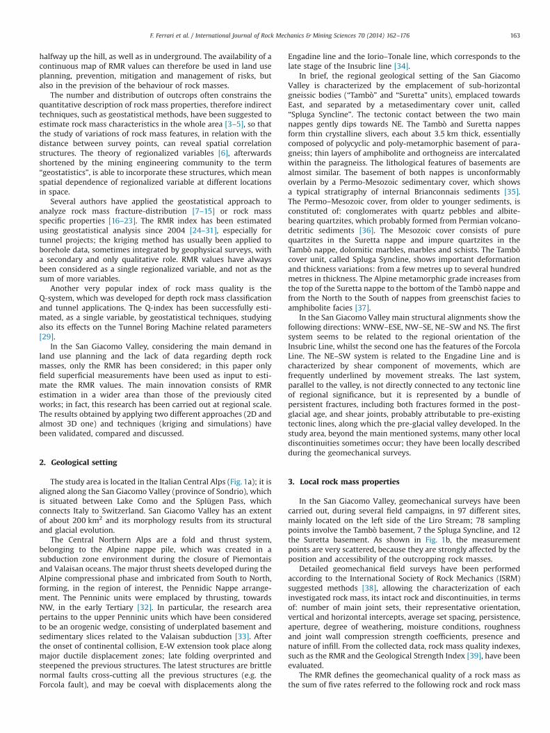
The results (Fig. 2) show a high variability of JCS values, whichare very scattered and range from 35 to 216 MPa, although theoutcropping rocks are almost all paragneiss. It follows that in thestudied area, the lithology does not seem to play a significantcontrol on the JCS values, excepting the amphibolite lenses whichalways give high JCS values, which however are aligned and nothigher than the maximum paragneiss value. As a consequence, inthis area, the estimation of the JCS values, in each point of thedomain, constrained by the outcropping lithology, should lead tomeaningless results, also due to the lack of significant number ofsampling points for the lithologies, such as amphibolite andquartzite, which outcrop only sporadically, in small lenses or inveins and so in very localized zones.

3.2. Rock quality designation (RQD)

The second parameter used to calculate RMR has been indir-ectly derived, due to the lack of cores referred to in the surveylocation. Palmstrom [40] has suggested that, when cores areunavailable, the RQD may be estimated from the number of jointsper unit of volume, in which the number of discontinuities permetre for each joint is added. The conversion formula for clay-freerock masses is as follows:

RQD¼ 115–3:3Jv ð2Þwhere Jv is the Volumetric Joint Count, which represents the totalnumber of joints within a unit of volume of rock mass and can bederived from the average spacing of each discontinuity set:

Jv¼ 100=SK1þ100=SK2þ⋯þ100=SKn ð3Þwhere S is the joint spacing, in centimetres, for each joint set Kn.Since Jv is based on joint measurements of spacings or frequencies,it can be easily calculated.

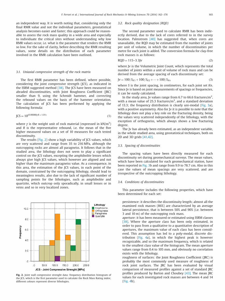
In the study area, Jv values range from 6.7 to 66.6 fractures/m3,with a mean value of 25.3 fractures/m3, and a standard deviationof 13.3; the frequency distribution is clearly uni-modal (Fig. 3a),with a positive asymmetry. Also for Jv it is possible to note that thelithology does not play a key role on the fracturing density, beingthe values very scattered independently of the lithology, with theexception of orthogneiss, which always shows a low fracturingdegree.

The Jv has already been estimated, as an independent variable,in the whole studied area, using geostatistical techniques, both on2D and 3D grids [41,42].

3.3. Spacing of discontinuities

The spacing values have been directly measured for eachdiscontinuity set during geomechanical surveys. The mean values,which have been calculated for each geomechanical station, havebeen reported in Fig. 3b and range from 9.9 to 78.7 cm. Also in thiscase the values of mean spacings are very scattered, and areirrespective of the outcropping lithology.

3.4. Conditions of discontinuities

This parameter includes the following properties, which havebeen determined for each set:

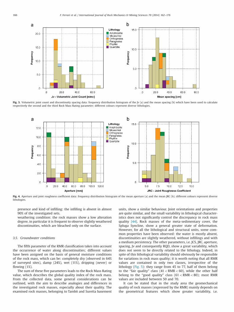
persistence: it describes the discontinuity length; almost all theexamined rock masses (86%) are characterized by an averagelateral persistence, that is between 50% and 90% (i.e. between3 and 10 m) of the outcropping rock mass.aperture: it has been measured or estimated using ISRM classes[38]. Where the aperture class has been only estimated, inorder to pass from a qualitative to a quantitative description ofapertures, the maximum value of each class has been consid-ered. This assumption has led to a poly-modal, discrete dis-tribution (Fig. 4a), in which the highest peak is howeverrecognizable, and so the maximum frequency, which is relatedto the smallest class value of the histogram. The mean aperturevalues range from 0.4 to 105 mm, and obviously no correlationexists with the lithology.roughness of surfaces: the Joint Roughness Coefficient (JRC) isprobably the most commonly used measure of roughness ofrock joint surfaces. The JRC has been evaluated by visualcomparison of measured profiles against a set of standard JRCprofiles produced by Barton and Choubey [43]. The mean JRCvalues for each investigated rock masses are between 4 and 14(Fig. 4b).

Fig. 2. Joint wall compressive strenght data: frequency distribution histogram ofthe JCS, which is the first parameter used to calculate the Rock Mass Rating index;different colours represent diverse lithologies.

F. Ferrari et al. / International Journal of Rock Mechanics & Mining Sciences 70 (2014) 162–176 165

presence and kind of infilling: the infilling is absent in almost90% of the investigated sets.weathering condition: the rock masses show a low alterationdegree, in particular it is frequent to observe slightly weathereddiscontinuities, which are bleached only on the surface.

3.5. Groundwater conditions

The fifth parameter of the RMR classification takes into accountthe occurrence of water along discontinuities; different valueshave been assigned on the basis of general moisture conditionsof the rock mass, which can be: completely dry (observed in 64%of surveyed sites), damp (24%), wet (11%), dripping (never) orflowing (1%).

The sum of these five parameters leads to the Rock Mass Ratingvalue, which describes the global quality index of the rock mass.From the collected data, some general considerations can beoutlined, with the aim to describe analogies and differences inthe investigated rock masses, especially about their quality. Theexamined rock masses, belonging to Tambò and Suretta basement

units, show a similar behaviour. Joint orientations and propertiesare quite similar, and the small variability in lithological character-istics does not significantly control the discrepancy in rock massquality [44]. Rock masses of the meta-sedimentary cover, theSpluga Syncline, show a general greater state of deformation.However, for all the lithological and structural units, some com-mon properties have been observed: the water is mostly absent,discontinuities are slightly weathered, without infillings and witha medium persistency. The other parameters, i.e. JCS, JRC, aperture,spacing, Jv and consequently RQD, show a great variability, whichdoes not seem to be directly related to the lithology. Indeed, inspite of this lithological variability should obviously be responsiblefor variations in rock mass quality; it is worth noting that all RMRvalues are contained in only two classes, irrespective of thelithology (Fig. 5): they range from 45 to 77, half of them belongto the “fair quality” class (41oRMRo60), while the other halfbelong to the “good quality” class (61oRMRo80); most RMRvalues are included between 50 and 70.

It can be stated that in the study area the geomechanicalquality of rock masses (expressed by the RMR) mainly depends onthe geometrical features which show greater variability, i.e.

Fig. 3. Volumetric joint count and discontinuity spacing data: frequency distribution histogram of the Jv (a) and the mean spacing (b) which have been used to calculaterespectively the second and the third Rock Mass Rating parameter; different colours represent diverse lithologies.

Fig. 4. Aperture and joint roughness coefficient data: frequency distribution histogram of the mean aperture (a) and the mean JRC (b); different colours represent diverselithologies.

F. Ferrari et al. / International Journal of Rock Mechanics & Mining Sciences 70 (2014) 162–176166

spacing and correlated values of Jv and RQD [45], JCS andconditions of discontinuities (with particular reference to apertureand roughness). These properties, which are related to tectonicactions, could be considered as regionalized variables, as RMR.Actually, the RMR depends on the geological and structural historyof the rock mass, but it describes the quality of the rock massnowadays, resulting from all the involved geological events. TheRMR is a global property of rock masses, depending on all itsfractures, despite of their formation mechanism. Therefore thestatistical population of RMR is represented from all the rockmasses outcropping in the San Giacomo Valley. The homogeneityof the data samples has been guaranteed, because the samesupport (a scanline 20 m long) has been used in all the geome-chanical surveys, with a surveyed height of about 2 m.

4. Geostatistical analysis

Geostatistics allows estimating the values of regionalized variablesin un-sampled points, capturing the spatial correlation among data,based on the fact that the data sourced from closer locations tend to be

more similar than those far apart. Geostatistics provides an unbiasedestimation, with uncertain quantification.

Geostatistical approach has been already used several timesin rock mass characterization [7–31]. In this paper, geostatisticalanalysis has been performed in order to reconstruct the values ofRMR in an area with an extent of approximately 200 km2, fromsuperficial field data. The geostatistical study has been performedwith the RMR index as regionalized variable and has beendeveloped by the following phases: exploratory spatial dataanalysis, variography, prediction and finally validation.

4.1. Exploratory spatial data analysis

First of all, the statistical parameters of RMR have beencomputed. The RMR index has been evaluated in 55 differentlocations, along the San Giacomo Valley. RMR values range from45 to 77, the mean is 60.6, with a standard deviation of 6. Thefrequency distribution seems to be Gaussian, indeed it is clearly aunimodal distribution, without a significant asymmetry (Fig. 6a),being both skewness and kurtosis close to zero.

Since many geostatistical techniques are more reliable if thevariable of interest has a standard Gaussian distribution, it isnecessary to verify if the variable has a normal distribution and ifnot the transformation of data into a standard Gaussian one isessential. It is rare in the modern geostatistics to consideruntransformed data. The use of Gaussian technique requires aprior Gaussian transformation of data and the reconstruction ofsemivariogram model on these transformed data. This transforma-tion has some important advantages: the difference betweenextreme values is dampened and the theoretical sill should beclose to the unit [46]. Furthermore systematic trends should beremoved from the variable prior to transformation and semivar-iogram calculation.

The problem is that the most common statistical tests, used toverify if the univariate distribution of the data is Gaussian, aredesigned on the assumption that the observations are indepen-dent and identically distributed. In geostatistical applications,however, this is not usually the case: if the covariance structurehas a range greater than the minimum distance between observa-tions, the data are correlated and the standard tests cannot beapplied to the probability density function (pdf) or cumulativeprobability function (cdf) estimated directly from the data.The problem with correlated data arises not from the correlationper se, but from cases in which correlated data are clustered ratherthan being located on a regular grid [47]. When preferentialsampling occurs, observations that are close together provide

Fig. 5. Rock Mass Rating values: frequency distribution histogram of the Rock MassRating; different colours represent diverse lithologies.

Fig. 6. Rock Mass Rating values: frequency distribution histogram of raw (a) and transformed (b) data, with superimposed the Gaussian distribution (solid line).

F. Ferrari et al. / International Journal of Rock Mechanics & Mining Sciences 70 (2014) 162–176 167

partially redundant information that must be taken into account incalculating pdf or cdf. Actually, it is difficult and often impossibleto sample geological data using a regular grid; therefore theoccurrence of preferential sampling is very frequent. For instance,in this case study, the sampling locations are dependent on theoutcrop positions and their accessibility; hence they are notdisposed on a regular grid.

The preferential sampling could lead to the presence of spatialclusters, and subsequent biases. When the sampling is clustered,unbiased estimates of pdf or cdf must first be obtained, by de-clustering, then normality tests can be applied. In this case study,the analysis of the spatial disposition of 55 considered datalocations has been performed through the nearest neighbourindex, which uses the distance between each point and its closestneighbouring point to determine if the point pattern is random,regular or clustered. The nearest neighbour index is expressed bythe average distance between each point and its nearest neigh-bours, divided by the expected distance (i.e. the average distancebetween neighbours in a hypothetical random distribution). If theindex is less than 1, the pattern exhibits clustering; if the index isgreater than 1, the trend is towards dispersion or competition. Inthis case study the index is equal to 1, with a standard deviation of0.03, showing that the pattern of sampling locations is neitherclustered nor dispersed. Therefore the data de-clustering is notnecessary and has not been performed.

The normality of RMR distribution has been verified usingvarious graphical and statistical tests, such as Shapiro–Wilk test[48] and Kolmogorov–Smirnov test with Lilliefors correction [49];hence the Gaussian distribution of RMR has been confirmed with asignificance level of 1%.

Since the standard Gaussian distribution, with mean andvariance equal to 0 and 1, respectively, is required, the Gaussiandistribution of RMR has been transformed in a standard one(Fig. 6b), through a process called Gaussian anamorphosis.

As many geostatistical methods are based on the spatialstationarity property, the absence of systematic trends has to beverified. The study of trends, which has been carried out repre-senting the magnitude of variable along different directions in thespace, has allowed us to confirm the stationarity hypothesisof RMR in the studied domain. In particular the absence of trendallows applying the kriging without trend, which accounts forlocal fluctuations of the mean limiting the domain of stationarityof the mean to the local neighbourhood centred on the locationunder estimation [50].

4.2. Variography

The variography is based on the modelling of semivariogram,which is the tool that permits to individuate the occurrenceof some spatial structure in the dataset. The construction ofsemivariogram, that is the mathematical model which capturesthe spatial correlation among data, is a very important step inany geostatistical analysis. The semivariogram is a measure ofvariability, it increases as samples become more dissimilar.The variogram is defined as the expected value of a squareddifference [51]:

2γðhÞ ¼ Var½ZðxÞ�ZðxþhÞ� ¼ EfZðxÞ�ZðxþhÞ�2g ð4Þwhere Z is a stationary random function with known mean m andvariance s2, which is independent of location, so m(x)¼m ands2(x)¼s2 for all locations x in the study area, therefore thevariogram function depends only on the distance h and so theintrinsic hypothesis occurs.

The variogram is a graph that can be obtained by plotting thedistance among sampling points (called lag) on x-axis, versus theassociated variance, on the y-axis. The variogram therefore is the

expected squared difference between two data values separatedby a distance vector. The semivariogram γ(h) is one half ofvariogram 2γ(h), to avoid excessive jargon in this paper we simplyrefer to it with the term variogram.

If a variable is correlated, initially the variogram increases andthen becomes stable beyond a distance h called range. Beyond thisdistance, the mean square deviation between two quantities Y(u)and Y(uþh) no longer depends on the distance h between themand the two quantities are no longer correlated. When the range isdifferent in some directions of space, the examined regionalizedvariable exhibits a geometric anisotropic structure. The rangecorresponds to a variance value called sill, which corresponds tozero correlation. Briefly the variogram quantifies the distance(range) at which samples become uncorrelated from each other,giving an idea of the best and the worst spatial correlationdirections among the data. The former occurs where the range ismaximum, the latter has been assumed perpendicular to themaximum correlation direction.

The computation of the variogram is based on the MeanErgodic Hypothesis [52] that permits the substitution of thestochastic mean value with the mean value of all the couples ofmeasurement points that are approximately h distance apart. Thisimplies that the process is regular or statistically homogeneous toensure that, from a unique realization of the process, there is arepresentation of all possible values that the process can attain.Actually, the mean value of the regionalized variable does notdepend on its spatial position, but on the distance from therealizations.

A random function is mean-ergodic if the process has finitevariance: the process may be assumed to be distribution-ergodic ifthe indicator covariance function tends to zero for a distanceknown as the (practical) range of the covariance, and this distanceis much smaller than the maximum distance inside the considereddomain. It follows that the semivariogram must reach a sill, withina finite distance [47]. This condition can be used to checkexperimentally the distribution-ergodic hypothesis. In this casestudy, the experimental variograms (Table 1) do not have a drifteffect (i.e. they are not monotone ascending), but present a sill;hence the ergodic hypothesis is respected.

In practice, the process is not observed over an infinite domainbut over a finite domain of interest. The ergodicity explains theinevitable fluctuations of statistics and their consequences onmodelling. These ergodic fluctuations are due to the limited, finiteextent of the spatial domain being simulated. Simulation on aninfinitely large domain will result in statistics of realization thatexactly match the model statistics. Therefore, when simulating ona finite domain, some statistics have smaller variations than other.Ergodicity therefore plays an important role in both the estimationof model parameters as well as their simulation [53]. It is typicallyadvised in traditional geostatistical practice not to use any lagdistance information beyond 1/2 the size of the field, since theyare not reliable (not enough samples to provide a reliable vario-gram), and this statement has been observed in this work.

Variography has been applied here to recognize the RMRspatial distribution of the examined rock masses. An interpretationof variograms able to give a complete answer to the geologicalphenomena occurred in the studied area is truly difficult andcomplex, being San Giacomo Valley located in an alpine dynamiccontext, which does not have a simple geological history, with thesuperimposition of numerous short time events with majorprocesses acting on geological time scales. However it is easy tounderstand that geological characteristics that have beenformed in a slow and steady geological environment are bettercorrelated to each other than if they had been results of an oftenabruptly changing geological process [54], such as in theresearch area.

F. Ferrari et al. / International Journal of Rock Mechanics & Mining Sciences 70 (2014) 162–176168

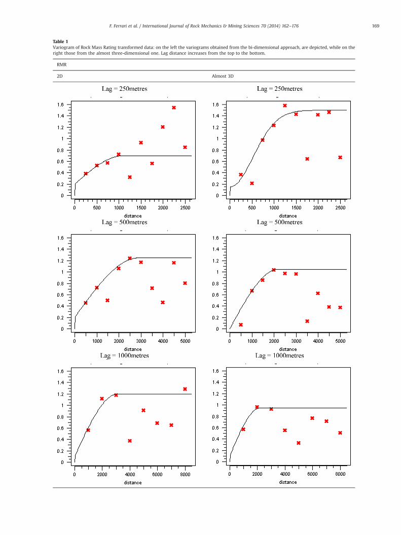
Table 1Variogram of Rock Mass Rating transformed data: on the left the variograms obtained from the bi-dimensional approach, are depicted, while on theright those from the almost three-dimensional one. Lag distance increases from the top to the bottom.

RMR

2D Almost 3D

F. Ferrari et al. / International Journal of Rock Mechanics & Mining Sciences 70 (2014) 162–176 169

The variogram has been constructed using transformed data,with the support of the Stanford Geostatistical Modelling Software(SGeMS) [55]. The correlation structures of RMR have beeninvestigated at different scale and the possible occurrence ofanisotropies has been taken into account.

First of all an omni-directional variogram, which relates thedistance among pairs of sampling points with their variance, hasbeen constructed in order to individuate if a correlation of thevariable in the research area exists. The presence of any prefer-ential correlation direction has been first sought graphically usinga 2D variogram map, which is a plot of experimental variogramvalues in a coordinate system (hx; hy) with the centre of the mapcorresponding to the variogram at lag (0; 0) [50]. A more detailedresearch of maximum correlation direction has been conductedthrough the construction of several directional variograms, with avariation direction of 451 and an angular tolerance of 22.51.

Three experimental variograms have been constructed atdifferent scales, varying the lag distance from 250 to 1000 m,and therefore increasing the maximum distance under study. Thelag tolerance has been assumed equal to the half of lag distance.

A good regionalized variable should show an invariance ofscale: variograms should not depict important changes varying thescale, the structure and the maximum correlation direction shouldremain approximately the same [41], although small heterogene-ities, which are neglected in the variograms with large lag, couldbe better highlighted in the variograms created with small lag.

Experimental variograms have been determined using botha classical 2D approach and an almost 3D one: in the former thedistance among pairs of samples depends only on latitude andlongitude, in the latter, altitude also contributes to the distanceand it should play an important role where elevation gradients areworthy of note, such as in the study area. When the approachchanges, the maximum correlation direction becomes slightlydifferent: in the 2D approach it is towards NNE (22.51–202.51),whist in almost 3D one it has a dip direction toward NE (451) anddip of about 201, this orientation is in accordance with thediscontinuity set developed parallel to the regional foliation,which dips towards East with a low dip angle, and therefore hasa remarkable geological significance. Nevertheless, there are someanalogies between the two different approaches, withthe variableunder study being the same. First of all, almost all the experi-mental variograms are better fitted by a spherical theoreticalmodel; therefore variance values increase with the lag; thisindicates that the variability of RMR increases as the distance hamong sampling points grows and so that RMR is a regionalizedvariable.

The variogram models do not tend to zero when h is zero; thisdiscontinuity of variogram at the origin, which corresponds to theshort scale variability, is called nugget effect and can be due to local

heterogeneities of the geology structures, with correlation rangesshorter than the sampling resolution, or to measurements errors; it isworth noting that the nugget effect of all variograms is close to zeroand it is bigger in the 2D approach, this could be related to the factthat altitude of sampling point is neglected in the 2D approach.Actually such small nugget effect is also because the support of themeasure (equal to 20 m) is significantly smaller than the range.

Regarding the sill, its maximum admitted value is a debatedtopic, which has been considered by several authors [46,50,56,57];some scientists support that the maximum sill value should beequal to the variance, and thus to the unit in transformedvariables, while others admitted a sill value bigger than thevariance. In this geostatistical analysis model with a maximumsill both equal to sample variance and bigger than the samplevariance has been constructed. Since the validation shows that, inthis case, the sill greater than the unit provides the best results, inthe following phases only the model with the sill bigger than thesample variance has been considered and described. The experi-mental variograms show that generally the sill decreases whenlag distance increases, because the small heterogeneities areneglected and consequently the variance reduces. Finally, respectthe range, it is possible to notice that maximum range increaseswith lag distance, because the distance considered is longer, whileminimum range decreases.

Experimental and derived theoretical variograms, along themaximum correlation direction, obtained using different lag sizes,are shown in Table 1, while Table 2 reports the parameters used tocreate the variogram models.

4.3. Prediction

The prediction allows us to estimate RMR values in a wholedomain. In the 2D approach, the prediction has been carried outusing a grid which represents the study area in terms of longitudeand latitude, while in the 3D model altitude has also beenconsidered. Since borehole data are not available, the RMR indexhas been estimated only on the topographic surface and not indepth. The used grid is defined by regular square or cubic cells,100 m long for each side.

The parameters of the described theoretical variograms havebeen employed for the spatial interpolation of RMR values, initiallyby means of kriging technique. Among different kriging methods,several authors [25,27,30] have used indicator kriging to estimateRMR classes, but since in the study area RMR values fall withinonly two classes, instead of the categorical approach of indicatorkriging, the numerical one of ordinary kriging has been chosen.Furthermore the indicator kriging needs an indicator transforma-tion, which always implies a loss of information: the extrainformation about significant high or low values which fall withinthe same class is lost, actually whether a value is only a littlebigger or very bigger than the chosen threshold does not play arole. The ordinary kriging, which has been already used two timesin the RMR estimation [26,31], has been chosen to take in accountthe entire data set. The ordinary kriging is the technique thatprovides the Best Linear Unbiased Estimator of unknown fields[56,58], furthermore this method is a local estimator that providesthe interpolation and extrapolation of the originally sparselysampled data in the whole domain, assuming that the values arereasonably characterized by the Intrinsic Statistical Model.

Since RMR shows a strong spatial anisotropy, measurementsinside an elliptic research region, with axes parallel to maximumand minimum correlation directions (individuated by the direc-tional variograms), have been considered to perform the estima-tion process. In order to take into account the irregularity of datadistribution, the axes of ellipse have been computed as the doubleof ranges. Inside each ellipse a minimum of five and a maximum of

Table 2Variogram model parameters: the summary of values obtained by modellingexperimental variograms.

Lag¼250 m Lag¼500 m Lag¼1000 m

2D approachNugget effect 0.2 0.2 0.1Sill 0.7 1.25 1.2Maximum range (m) 1100 2900 3100Minimum range (m) 400 300 200

Almost 3D approachNugget effect 0.15 0 0.1Sill 1.5 1.05 0.95Maximum range (m) 1300 2200 2200Minimum range (m) 700 700 200

F. Ferrari et al. / International Journal of Rock Mechanics & Mining Sciences 70 (2014) 162–176170

20 data were considered; if in one research region there were lessthan five data the estimation was not performed, because theassociated variance would be too high.

The plausibility of the interpolation models has been investi-gated using a cross-validation procedure, which consists of sequen-tial estimation at each of n known locations using remaining n�1sampled locations of the domain. This analysis, which comparesestimates and actual known sampled values, shows that theestimation method adopted tends to overestimate low values andunderestimate high ones, producing a marked smoothing effect,which leads to neglect the extreme values of sample distributionand therefore does not preserve the variability of parameters underinvestigation. The cross-validation also shows that the smoothingeffect is bigger in almost 3D models than in 2D ones. The modelimpacts of the smoothing effect are not very strong when themodelled parameter shows a low variability, but more variable thegeology is, stronger the impacts of smoothing effect will be [54]. Inan Alpine area, such as San Giacomo Valley, the smoothing effect isremarkable, therefore a method which avoids this effect is prefer-able. Geostatistical simulation techniques generate models withoutsmoothing effect, taking into account the spatial variability ofregionalized variable. This method does not provide the best linearunbiased estimate, but it creates realizations with the samevariability as that observed in the field [6].

Gaussian sequential simulation has been performed usingparameters of spatial continuity models previously defined

through variogram analysis and the same grid and research ellipseas of those used in the ordinary kriging. Gaussian sequentialsimulation is a conditional method, which is forced to assumethe measured values of the variable in the sampling points.Geostatistical simulations (or stochastic representations) can beseen as possible realizations of a spatially correlated random field,they all honour the spatial moments (mean, variance) of the field.Each simulation delivers a different realization, therefore simula-tions do not provide good local estimators but they are gooddescriber of spatial uncertainty. Various realizations might initiallyseem to be quite different; nevertheless the variability anddistribution of estimated values are very similar to those of theoriginal data, and the smoothing effect, which has been observedusing the kriging method, does not occur. Even if each simulationmaintains the variability and distribution of samples, it provides adifferent map; hence in order to get a final map, it is necessary tocalculate, in each location of the grid, a single estimated value ofleast squared error-type: the conditional expectation.

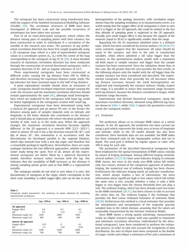
Fig. 7 compares the estimated RMR values obtained by the krigingapproach (Fig. 7a) and sequential Gaussian simulation technique(Fig. 7b), through the almost 3D model with lag of 500 m.Un-estimated areas (white regions in Fig. 7a) are due to ellipticalresearch region with less than five samples. The two resulting mapsare quite different and the main points discussed for the 2D predictionare still valid. Moreover the 3D kriging map appears much morecontinuous than the simulation map, which allows abrupt local

Fig. 7. Expected Rock Mass Rating values: the map of RMR values estimated using ordinary kriging (a) and sequential Gaussian simulation (b), with almost three-dimensional approach and medium lag.

F. Ferrari et al. / International Journal of Rock Mechanics & Mining Sciences 70 (2014) 162–176 171

variation; the 3D simulation seems to better count for the geologicalsettings and topography than the 2D simulation.

The optimal number of simulations has been chosen comparingthe results of 10, 100 and 1000 simulations, through a validationprocess. In the present study the optimal number of simulationshas resulted to 100, because it provides the best compromisebetween the accuracy of results and the computation time.

Ordinary kriging and sequential Gaussian simulations providequite similar outcomes for the central values of variable frequencydistribution, while remarkable differences occur for the extremevalues of data, indeed these values are neglected in the krigingresults, while they are maintained in those coming from Gaussiansimulation technique.

4.4. Validation

With the aim of comparing results obtained from the two differentgeostatistical techniques, a validation process has been performed,using an independent data set. About 10 new geomechanical surveyshave been carried out in the research area to form the training pointdata set.

The validation process has been performed comparing mea-sures of new sampling points with estimated values in theirlocations. The difference between actual and estimated valueshas allowed computing the following parameters (for each appliedtechnique): mean error and its related root-mean-square, averagestandard error, mean standardized error and root-mean-squarestandardized error.

In 2D models the minimum mean error has been obtained byperforming kriging on the longest lag distance (equal to 1000 m),while the minimum standard deviation of errors comes fromsequential Gaussian simulation technique also based on 1000 mlag distance. Generally the validation reveals a quite good agree-ment between measured and estimated data in new samplinglocations, the results of sequential Gaussian simulation are lightlybetter than those obtained from ordinary kriging. Neverthelesskriging results obtained from a 2D grid are better than thoseobtained from an almost 3D one. Overall the best results comefrom sequential Gaussian simulation, implemented on a 3D grid,with a medium lag distance (equal to 500 m), which representsthe best compromise between small and big heterogeneitiesconsidered by the variogram. Actually, the almost 3D approachshows a notable difference between ordinary kriging and sequen-tial Gaussian simulation results, being the smoothing effect of

kriging very high, indeed only the central values are exactlyestimated with kriging method.

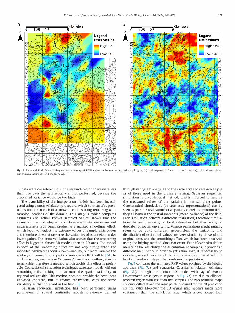
A brief visual summary of the results is shown in Fig. 8, thegraph relates measured and estimated values of new samplingpoint dataset; the bisector is the place of points where theestimated values are equal to the measurements, the line closerto the bisector, is the regression line obtained from the sequentialGaussian simulation with medium lag and 3D grid.

5. Discussion and further improvement in prediction

Although the validation process shows a quite good agreementbetween estimated and measured RMR values, the resulting maps(Fig. 7) do not seem to properly count for the geometric relationbetween geological and structural setting and topography.Although the almost 3D approach shows a good improvement,the topography seems to only lightly affect the map, actually insome zones the RMR values are irrespective of isohypses, althoughthe variograms have a low angle of dip. The model might beaffected by such a parameter of the RMR sum, not adequatelydescribed and poor correlated. All the RMR parameters implygeometric features, with the exception of the groundwater condi-tion. It is worth to note that, although the RMR classification wasborn especially in reference to the underground rock massesinvolved in tunnelling, and so to the groundwater circulation,during the geomechanical surveys the external moisture condi-tions of rock mass are revealed; these conditions are affected bythe local climatic situations of the days before the survey,especially in Alpine areas where the weather can be very change-able. Furthermore in the research area the presence of water wassurveyed with very different conditions from site to site: thesurveys have been carried out during different seasons and hencewith several climatic and weather situations; in particular in SanGiacomo Valley, as well in all Alpine valleys characterized by heavysnows in winter, the presence of water differs enormously fromweek to week, according to the global snow-melt regime. Conse-quently this parameter has not been surveyed in standard condi-tions and therefore could not be represented and properlyintroduced in the geostatistical analysis. With the aim to uniformthe weight related to the presence of water, considering that 64%of the investigated rock masses were completely dry during thesurveys and only 1% showed flowing condition, all RMR values

Fig. 8. Validation of results: the graph associates measured Rock Mass Ratingvalues with the estimated ones in new sampling locations, and compares twodifferent techniques (kriging and simulation) and approaches (bi-dimensional andalmost three-dimensional).

Fig. 9. Rock Mass Rating values in dry conditions: frequency distribution histogramof the Rock Mass Rating calculated with the absence of water; different coloursrepresent diverse lithologies.

F. Ferrari et al. / International Journal of Rock Mechanics & Mining Sciences 70 (2014) 162–176172

have been computed again with the assumption that all rockmasses were dry during the survey campaigns and so attributing15 points to the last RMR parameter. The “dry RMR” values

obviously are higher than the previous RMR values, although theyfall again in the “fair” and “good” quality classes (Fig. 9): the meanand median values are slightly higher than those computedconsidering the water, whilst the extreme values, referred to dryrock masses, do not change. The distribution shows a negativeasymmetry, so the Gaussian anamorphosis has been performedonce again in order to apply geostatistical techniques.

The transformed data have been used to compute directionalvariograms, applying the almost 3D approach, which has alreadyproven to be the most effective. The maximum correlation direc-tion is slightly rotated towards East and it exactly coincides withthe mean discontinuity set developed parallel to the regionalfoliation, while the dip angle is equal to 101. The invariance ofscale has also been observed using the “dry RMR” data. The

Table 3Variogram model parameters: summary of values obtained by modelling experi-mental variograms of “dry RMR” values.

Lag¼250 m Lag¼500 m Lag¼1000 m

Almost 3D approachNugget effect 0 0 0Sill 1.5 1.2 1.1Maximum range (m) 2300 3300 3600Minimum range (m) 200 200 200

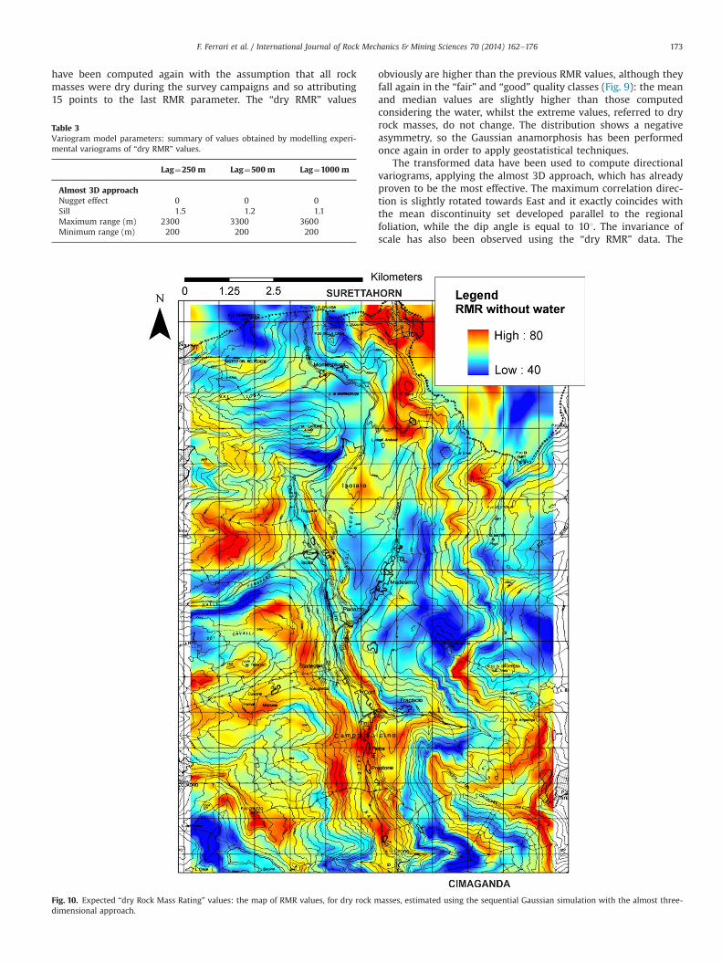
Fig. 10. Expected “dry Rock Mass Rating” values: the map of RMR values, for dry rock masses, estimated using the sequential Gaussian simulation with the almost three-dimensional approach.

F. Ferrari et al. / International Journal of Rock Mechanics & Mining Sciences 70 (2014) 162–176 173

theoretical models, which better fit the experimental variograms,are again spherical models for the variograms with bigger lags anda Gaussian model for the variogram with the shortest lag, whichtherefore shows a grater continuity than others. The features ofthe chosen variogram models are reported in Table 3.

All models confirm that when the lag increases the silldecreases, because increasing the distance the small heterogene-ities are neglected, consequently the variance reduces; on thecontrary the maximum range increases with lag distance, becausethe distance considered is longer. It is important to note thatthe nugget effect is equal to zero in all the variograms calculatedwithout water and it can be considered a good clue, becausetypically the nugget effect is related to measurement errors or toshort scale variability, with correlation range shorter than thesampling resolution, hence to the use of a not correct samplinggrid. Considering the rock masses dry, the nugget effect is removedand so the estimation results should be improved.

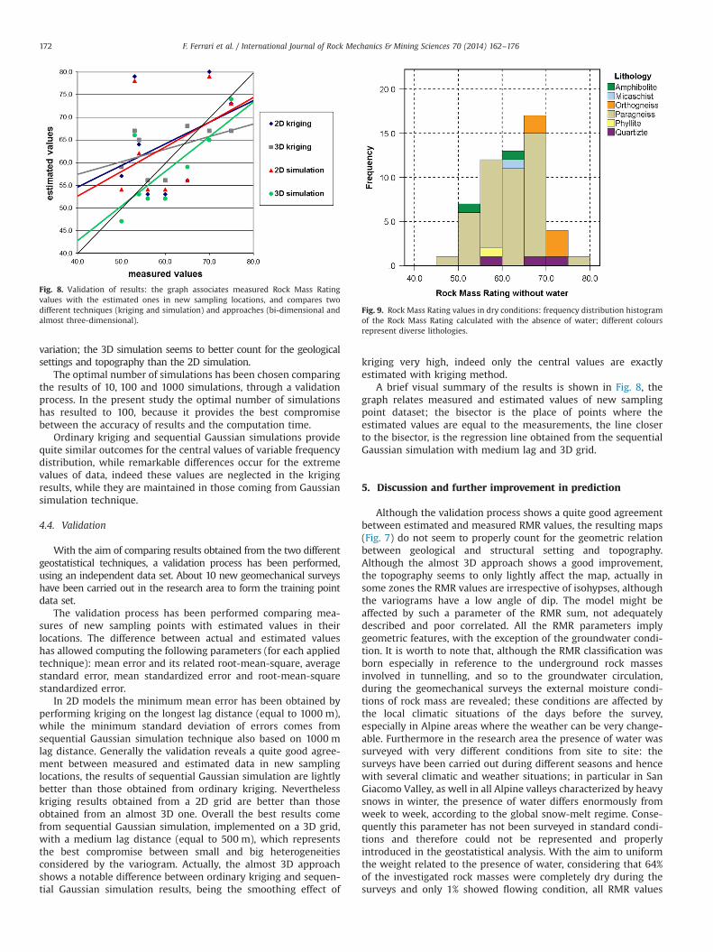
Only the results of the estimation performed by sequentialGaussian simulation, carrying out 100 realizations, on a 3D grid arepresented. The expected RMR values (Fig. 10) meet some impor-tant geological evidence: e.g. the low quality of rock masses, whichoutcrop on the South-East of the map with an arc shape,corresponds to the big niche of the historical Cimaganda landslide;the high quality of the Surettahorn rock masses, one of the highestmountains in Chiavenna Valley, on the North-East of the map,where the outcropping orthogneiss and migmatitic are character-ized by a very low schistosity and wide spacing.

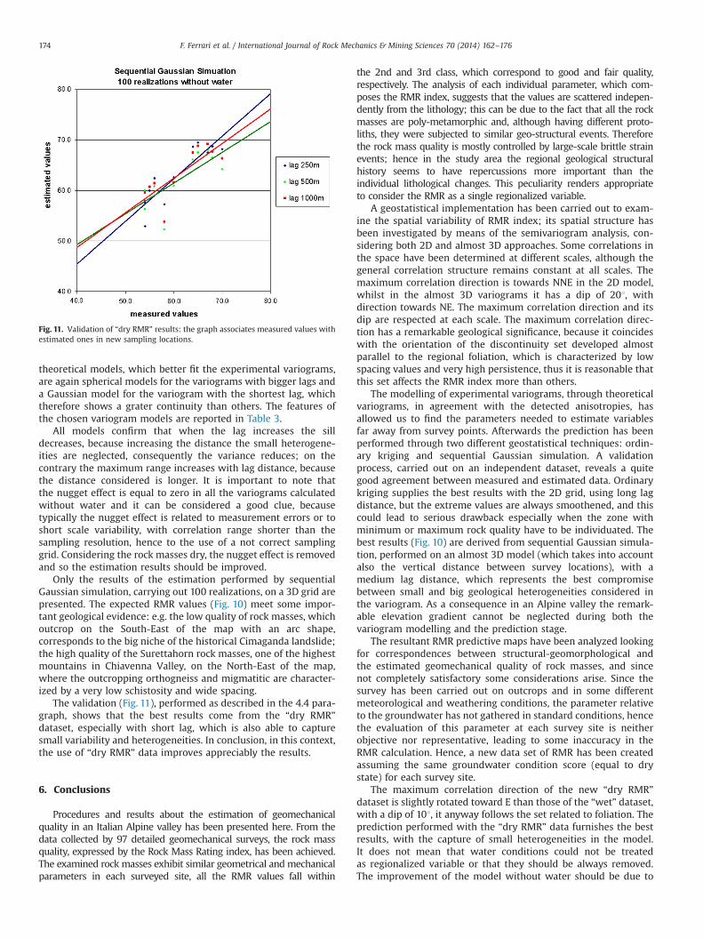
The validation (Fig. 11), performed as described in the 4.4 para-graph, shows that the best results come from the “dry RMR”dataset, especially with short lag, which is also able to capturesmall variability and heterogeneities. In conclusion, in this context,the use of “dry RMR” data improves appreciably the results.

6. Conclusions

Procedures and results about the estimation of geomechanicalquality in an Italian Alpine valley has been presented here. From thedata collected by 97 detailed geomechanical surveys, the rock massquality, expressed by the Rock Mass Rating index, has been achieved.The examined rock masses exhibit similar geometrical andmechanicalparameters in each surveyed site, all the RMR values fall within

the 2nd and 3rd class, which correspond to good and fair quality,respectively. The analysis of each individual parameter, which com-poses the RMR index, suggests that the values are scattered indepen-dently from the lithology; this can be due to the fact that all the rockmasses are poly-metamorphic and, although having different proto-liths, they were subjected to similar geo-structural events. Thereforethe rock mass quality is mostly controlled by large-scale brittle strainevents; hence in the study area the regional geological structuralhistory seems to have repercussions more important than theindividual lithological changes. This peculiarity renders appropriateto consider the RMR as a single regionalized variable.

A geostatistical implementation has been carried out to exam-ine the spatial variability of RMR index; its spatial structure hasbeen investigated by means of the semivariogram analysis, con-sidering both 2D and almost 3D approaches. Some correlations inthe space have been determined at different scales, although thegeneral correlation structure remains constant at all scales. Themaximum correlation direction is towards NNE in the 2D model,whilst in the almost 3D variograms it has a dip of 201, withdirection towards NE. The maximum correlation direction and itsdip are respected at each scale. The maximum correlation direc-tion has a remarkable geological significance, because it coincideswith the orientation of the discontinuity set developed almostparallel to the regional foliation, which is characterized by lowspacing values and very high persistence, thus it is reasonable thatthis set affects the RMR index more than others.

The modelling of experimental variograms, through theoreticalvariograms, in agreement with the detected anisotropies, hasallowed us to find the parameters needed to estimate variablesfar away from survey points. Afterwards the prediction has beenperformed through two different geostatistical techniques: ordin-ary kriging and sequential Gaussian simulation. A validationprocess, carried out on an independent dataset, reveals a quitegood agreement between measured and estimated data. Ordinarykriging supplies the best results with the 2D grid, using long lagdistance, but the extreme values are always smoothened, and thiscould lead to serious drawback especially when the zone withminimum or maximum rock quality have to be individuated. Thebest results (Fig. 10) are derived from sequential Gaussian simula-tion, performed on an almost 3D model (which takes into accountalso the vertical distance between survey locations), with amedium lag distance, which represents the best compromisebetween small and big geological heterogeneities considered inthe variogram. As a consequence in an Alpine valley the remark-able elevation gradient cannot be neglected during both thevariogram modelling and the prediction stage.

The resultant RMR predictive maps have been analyzed lookingfor correspondences between structural-geomorphological andthe estimated geomechanical quality of rock masses, and sincenot completely satisfactory some considerations arise. Since thesurvey has been carried out on outcrops and in some differentmeteorological and weathering conditions, the parameter relativeto the groundwater has not gathered in standard conditions, hencethe evaluation of this parameter at each survey site is neitherobjective nor representative, leading to some inaccuracy in theRMR calculation. Hence, a new data set of RMR has been createdassuming the same groundwater condition score (equal to drystate) for each survey site.

The maximum correlation direction of the new “dry RMR”dataset is slightly rotated toward E than those of the “wet” dataset,with a dip of 101, it anyway follows the set related to foliation. Theprediction performed with the “dry RMR” data furnishes the bestresults, with the capture of small heterogeneities in the model.It does not mean that water conditions could not be treatedas regionalized variable or that they should be always removed.The improvement of the model without water should be due to

Fig. 11. Validation of “dry RMR” results: the graph associates measured values withestimated ones in new sampling locations.

F. Ferrari et al. / International Journal of Rock Mechanics & Mining Sciences 70 (2014) 162–176174

different sampling conditions encountered during the surveys,which affect the datum. Actually supposing that all rock masseswere dry, the nugget effect, which is often related to measurementerrors, has been removed. Certainly in standard sampling situa-tions and in areas with steady meteorological conditions watercould be considered as the other parameter which composes theRMR and not separately.

In summary, geostatistical methods allow us to forecast thedistribution of RMR values far away from the points of survey, in avery extent area. In Alpine region the best geostatistical techniqueseems to be the sequential Gaussian simulation founded on analmost 3D variogramwhose anisotropy has to find correspondenceto the geological features. Therefore simulations should be per-formed on the 3D domain and always validated with an indepen-dent data set. The resultant predictive map should reveal a relationwith the regional geological and geomorphologial features ofthe area.

Acknowledgements

The research was financially supported by the Italian Ministryof Education, University and Research through the programmeResearch Project of National Interest (PRIN), and an Italian Minis-terial PhD scholarship (2007). Thanks to the Valchiavenna Com-munity, and to the colleagues Marco Masetti, Giovanni PietroBeretta and Alessio Conforto.

References

[1] Bieniawski ZT. Engineering rock mass classification. New York: Wiley; 1989.[2] Barton N, Lien R, Lunde J. Engineering classification of rock masses for the

design of tunnel support. Rock Mech 1974;6(4):189–236.[3] Isaaks EH, Srivastava RM. An introduction to applied geostatistics. Oxford:

Oxford University Press; 1989.[4] Villaescusa E, Brown ET. Characterising joint spatial correlation using geosta-

tistical methods. In: Barton N, Stephansson O, editors. Rock joints. Rotterdam:Balkema; 1990. p. 115–22.

[5] Giani GP. Rock slope stability analysis. Rotterdam: Balkema; 1992.[6] Matheron G. The theory of regionalized variables and its applications.

Fontainebleau: Ecole de Mines; 1971.[7] Long JCS, Billaux DM. From field data to fracture network modelling: an

example incorporating spatial structure. Water Resour Res 1987;23(7):1201–16.

[8] Young DS. Random vectors and spatial analysis by geostatistics for geotechni-cal applications. Math Geol 1987;19(6):467–79.

[9] Chilès JP. Fractal and geostatistical method for modelling a fracture network.Math Geol 1988;20(6):631–54.

[10] Billaux D, Chilès JP, Hestir K, Long J. Three-dimensional statistical modelling ofa fractured rock mass - an example from the Fanay-Augères mine. Int J RockMech Min Sci 1989;26(3-4):281–99.

[11] Grigarten E. 3-D geometric description of fractured reservoir. Math Geol1996;28(7):881–93.

[12] Meyer T, Einstein HH. Geologic stochastic modelling and connectivity assess-ment of fracture systems in the Boston area. Rock Mech Rock Eng 2002;35(1):23–44.

[13] Dowd PA, Xu C, Mardia KV, Fowell RJ. A comparison of methods for thestochastic simulation of rock fractures. Math Geol 2007;39(7):697–714.

[14] Koike K, Ichikawa Y. Spatial correlation structures of fracture systems forderiving a scaling law and modelling fracture distributions. Comput Geosci2006;32:1079–95.

[15] Rafiee A, Vinches M. Application of geostatistical characteristics of rock massfracture system in 3D model generation. Int J Rock Mech Min Sci 2008;45:644–52.

[16] La Pointe PR Analysis of the spatial variation in rock mass properties throughgeostatistics. In: Proceedings of the 21st US rock mechanics symposium, 1980;p. 570–80.

[17] Young DS. Indicator kriging for unit vectors: rock joint orientations. Math Geol1987;19(6):481–501.

[18] Yu YF, Mostyn GR. Spatial correlation of rock joints. Probabilistic methods ingeotechnical engineering. Rotterdam: Balkema; 1993.

[19] Tavchandjian O, Rouleau A, Archambault G, Daigneault R, Marcotte D.Geostatistical analysis of fractures in shear zones in the Chibougamau area:applications to structural geology. Tectonophysics 1997;269:51–63.

[20] Ozturk CA, Nasuf E. Geostatistical assessment of rock zones for tunnelling.Tunn Undergr Space Technol 2002;17:275–85.

[21] Escuder Viruete J, Carbonell R, Martí D, Pérez-Estaún A. 3-D stochasticmodelling and simulation of fault zones in the Albalá Granitic Pluton, SWIberian Variscan Massif. J Struct Geol 2003;25:1487–506.

[22] Gumiaux C, Gapais D, Brun JP. Geostatistics applied to best-fit interpolation oforientation data. Tectonophysics 2003;376:241–59.

[23] Ellefmo SL, Eidsvik J. Local and spatial joint frequency uncertainty and itsapplication to rock mass characterisation. Rock Mech Rock Eng 2009;42(4):667–88.

[24] Oh S, Chung H, Lee DK. Geostatistical integration of MT and borehole data forRMR evaluation. Environ Geol 2004;46:1070–8.

[25] You K, Lee JS. Estimation of rock mass classes using the 3-dimensionalmultiple indicator kriging technique. Tunn Undergr Space Technol 2006;21(3-4):229.

[26] Stavropoulou M, Exadaktylos G, Saratsis G. A combined three-dimensionalgeological-geostatistical-numerical model of underground excavations inrock. Rock Mech Rock Eng 2007;40(3):213–43.

[27] Choi JY, Lee CI An estimation of rock mass rating using 3D-indicator krigingapproach with uncertainty assessment of rock mass classification. In: Pro-ceedings of the 11th congress of the international society for rock mechanics,Lisbon, vol. 2, 2007; p. 1285–88.

[28] Exadaktylos G, Stavropoulou M. A specific upscaling theory of rock massparameters exhibiting spatial variability: analytical relations and computa-tional scheme. Int J Rock Mech Min Sci 2008;45:1102–25.

[29] Exadaktylos G, Stavropoulou M, Xiroudakis G, de Broissia M, Schwarz H.A spatial estimation model for continuous rock mass characterization from thespecific energy of a TBM. Rock Mech Rock Eng 2008;41:797–834.

[30] Choi Y, Yoon SY, Park HD. Tunneling analyst: a 3D GIS extension for rock massclassification and fault zone analysis in tunneling. Comput Geosci2009;35:1322–33.

[31] Kaewkongkaew K, Phien-wej N, Kham-ai D. Prediction of rock mass alongtunnels by geostatistics. In: Fuenkajorn, Phien-wej, editors. Rock mechanics;2011. p. 269–76.

[32] Froitzheim N, Schdmid ST, Conti P. Repeated change from crustal shorteningto orogenparallel extension in the Austroalpine units of Graubünden. EclogaeGeol Helvetiae 1994;87(2):559–612.

[33] Marquer D, Baudin TH, Peucat JJ, Persoz F. Rb–Sr mica ages in the Alpine shearzones of the Truzzo granite: timing of the tertiary alpine P–T deformations inthe Tambò nappe (Central Alps, Switzerland). Eclogae Geol Helvetiae 1994;85(3):1–61.

[34] Schmid SM, Zingg A, Handy M. The kinematics of movements along theinsubric line and the emplacement of the Ivrea zone. Tectonophysics1987;135:47–66.

[35] Baudin T, Marquer D, Barfety JC, Kerckhove C, Persoz F. A new stratigraphicalinterpretation of the mesozoic cover of the Tambò and Suretta nappes:evidence for early thin-skinned tectonics (Swiss Central Alps). ComptesRendus de l’ Acad des Sci Paris 1995;321(5):401–8.

[36] Huber RH, Marquer D. Tertiary deformation and kinematics of the southernpart of the Tambò and Suretta nappes (Val Bregaglia, Eastern Swiss Alps).Schweiz Min Petrogr Mitt 1996;76:383–97.

[37] Baudin TH, Marquer D. Metamorphism and deformation in the Tambò nappe(Swiss Central Alps): evolution of the phengite substitution during Alpinedeformation. Schweiz Min Petrogr Mitt 1993;73:285–99.

[38] ISRM. Suggested methods for the quantitative description of discontinuities inrock masses. Int J Rock Mech Min Sci 1978;15(6):319–68.

[39] Hoek E, Brown ET. Practical estimates of rock mass Strength. Int J Rock MechMin Sci 1997;34(8):1165–86.

[40] Palmstrom A The volumetric joint count: a useful and simple measure of thedegree of rock mass jointing. In: Proceedings of the IAEG congress, New Delhi,1982; p. V. 221–28.

[41] Ferrari F, Apuani T, Giani GP Geomechanical surveys and geostatisticalanalyses in Valchiavenna (Italian Central Alps). In: Proceedings of the8th international symposium on field measurement in geomechanics, Berlin;2011.

[42] Ferrari F, Apuani T, Giani GP. Analisi spaziale e previsionale delle proprietàgeomeccaniche degli ammassi rocciosi della Val San Giacomo (SO), mediantetecniche geostatistiche. GEAM – Geoing Ambient e Min 2012;1:21–30.

[43] Barton NR, Choubey V. The shear strength of rock joints in theory and practice.Rock Mech 1977;10(1–2):1–54.

[44] Apuani T, Giani GP, Merri A Geomechanical studies of an alpine rock mass. In:Proceedings of the 3rd CAN-US rock mechanics symposium, Toronto; 2009.

[45] Priest SD, Hudson JA. Discontinuity spacing in rock. Int J Rock Mech Min Sci1976;13(5):135–48.

[46] Grigarten E, Deutsch CV. Variogram interpretation and modelling. Math Geol2001;33(4):507–34.

[47] Pardo-Igùzquiza E, Dowd PA. Normality tests for spatially correlated data.Math Geol 2004;36(6):659–81.

[48] Shapiro SS, Wilk MB. An analysis of variance test for normality (completesamples). Biometrika 1965;52(3-4):591–611.

[49] Lilliefors HW. On the Kolmogorov–Smirnov test for normality with mean andvariance unknown. J Am Stat Assoc 1967;62(318):399–402.

[50] Goovaerts P. Geostatistics for natural resources evaluation. Oxford: OxfordUniversity Press; 1997.

[51] Isaaks E, Srivastava RM. An introduction to applied geostatistics. New York:Elsevier; 1989.

[52] Papoulis A. Probability, random variables and stochastic processes. Singapore:McGraw-Hill; 1984.

F. Ferrari et al. / International Journal of Rock Mechanics & Mining Sciences 70 (2014) 162–176 175

[53] Caers J, Zhang T. Multiple-point geostatistics: a quantitative vehicle forintegrating geologic analogs into multiple reservoir models, 80. Vancouver,Canada: American Association of Petroleum Geologists; 2004; 383–94.

[54] Marinoni O. Improving geological models using a combined ordinary-indicator kriging approach. Eng Geol 2003;69:37–45.

[55] Remy N, Boucher A, Wu J. Applied geostatistics with SGeMS: a user's guide.New York: Cambridge University Press; 2008.

[56] Journel AG, Huijbregts C. Mining geostatistics. London: Academic Press; 1978.[57] Barnes RJ. The variogram sill and the sample variance. Math Geol 1991;23

(4):763–8.[58] Kitanidis PK. Introduction to geostatistics: applications in hydrogeology.

Cambridge: Cambridge University Press; 1997.

F. Ferrari et al. / International Journal of Rock Mechanics & Mining Sciences 70 (2014) 162–176176