rock mass strength and slope stability of the hilina slump,...
TRANSCRIPT
www.elsevier.com/locate/jvolgeores
Journal of Volcanology and Geotherm
Rock mass strength and slope stability of the Hilina slump,
Kılauea volcano, Hawai‘i
Chris H. Okubo*
Geomechanics–Rock Fracture Group, Department of Geological Sciences/172, Mackay School of Earth Sciences and Engineering,
University of Nevada, Reno, NV, 89557-0138, United States
Received 26 August 2003; accepted 11 June 2004
Abstract
Stability of the Hilina slump, on the south flank of Kılauea volcano, Hawai’i, is investigated using slope stability analyses
based on rock mass mechanics. The Hilina slump is an active example of the giant landslides that are observed around
submarine flanks of ocean island volcanoes. Based on edifice topology, along with derived rock mass strength and
deformability parameters, slope stability analyses predict that the geometries of present-day failure surfaces of the Hilina slump
are shallow, located at less than ~3.5 km depth below the upper surface of the edifice. The failure surfaces at the base of the
Hilina slump are predicted to be structurally independent from a previously interpreted subjacent detachment at the contact
between the Kılauea edifice and the oceanic crust. Based on these model results, the Hilina slump is envisioned to ride atop the
south flank of Kılauea as it spreads seaward along this slipping basal detachment. Under present-day slope and sea-level
configurations, local horizontal ground accelerations greater than ~0.4–0.6 g are predicted to cause slip along failure surfaces
within Hilina slump. Therefore, dynamic stress changes due to slip along the subjacent detachment may potentially trigger slip
along failure surfaces of the Hilina slump. Model-derived stability and failure surface geometries can account for the distinct
observed distribution of slip along specific Hilina faults following the Mfa 7.9 1868 Ka’u and Ms 7.2 1974 Kalapana
earthquakes. Further, the spatial distribution of south flank aftershocks NM 1.5 recorded between 1950 and 1976 are consistent
with the predicted distribution of potential earthquake-induced slip of the Hilina faults.
D 2004 Elsevier B.V. All rights reserved.
Keywords: Kılauea volcano; Hilina slump; slope stability; geologic hazards; rock mechanics
0377-0273/$ - see front matter D 2004 Elsevier B.V. All rights reserved.
doi:10.1016/j.jvolgeores.2004.06.006
* Tel.: +1 775 784 6464; fax: +1 775 784 1833.
E-mail address: [email protected].
1. Introduction
Volcano slope stability has gained much attention
since the recognition of extensive landslide deposits
skirting islands of the Hawaiian Ridge (Moore et al.,
1989, 1994). Extensive landslide deposits have also
al Research 138 (2004) 43–76
C.H. Okubo / Journal of Volcanology and Geothermal Research 138 (2004) 43–7644
been mapped around ocean island volcanoes of the
Canary and Cape Verde islands (Carracedo, 1999;
Elsworth and Day, 1999) and Reunion (Duffield et al.,
1982; de Voogd et al., 1999). Catastrophic collapse of
volcano flanks has also been documented in terrestrial
settings, such as at Mount Shasta (Crandell, 1989),
Mount Rainier (Vallance and Scott, 1997) and Mount
St. Helens (Lipman and Mullineaux, 1981), and may
have been a significant process for volcanoes on other
planets (e.g., Lopes et al., 1982).
The Hilina slump, along the coastal south flank of
Kılauea volcano, Hawai’i, is an important example of
an active slope failure on a volcanic edifice. The head
region of the Hilina slump is subaerial and defined by
a population of arcuate, ocean-facing normal fault
scarps, which are collectively referred to here as the
Hilina fault system. The Hilina is significant because
of its long ~180-year history of first-hand observation
and its even longer ~43,000-year accessible geologic
record of fault offset. Active deformation along the
Hilina fault system has been recorded since early
European contact, most notably during earthquakes in
1823 (Ellis, 1827) and 1868 (Brigham, 1909).
Subsequent measurements of progressive deformation
during the 20th century led to hypotheses that the
Hilina fault system defines the head scarp of a largely
submerged active slump (Swanson et al., 1976; Tilling
et al., 1976; Lipman et al., 1985).
Deterministic methods for evaluating the stability
of a slope have been previously applied to volcanoes
(Iverson, 1995; Elsworth and Voight, 1995; Elsworth
and Day, 1999; Watters et al., 2000). In these studies,
field and laboratory measurements of rock mass
strength and groundwater conditions, along with
volcano topology, are incorporated into limit equili-
brium analyses in order to assess the stability of the
volcanic edifice.
In this paper, limit equilibrium analyses are used to
assess the stability of the Hilina slump. Results of these
analyses predict that the present-day failure surfaces
for the slump are within ~3.5 km below the upper
surface of Kılauea’s south flank. These results favor
previous interpretations that the Hilina slump rides
atop the south flank of Kılauea as it moves seaward,
along a slipping detachment at a sediment-rich inter-
face between the volcanic edifice and the underlying
Cretaceous-aged oceanic crust. Further, the Hilina
slump may do more than ride passively atop of the
moving south flank. Dynamic stress changes due to
slip along a basal edifice detachment are capable of
triggering slip along the failure surfaces of the Hilina
slump. Under present-day slope geometry and sea-
level conditions, horizontal ground accelerations
greater than ~0.4–0.6 g are predicted to promote
incremental slip along faults of the Hilina slump.
2. Approach
Kılauea volcano is composed of alternating sub-
aerial and submarine lava flows interbedded with
localized soil and tephra horizons (e.g., Stearns and
Macdonald, 1946; Eaton, 1987; Holcomb, 1987;
Wolfe and Morris, 1996). Lava flows are pervasively
fractured by cooling joints, and contacts between
flows are in general poorly welded. Loose clinker
surrounds the massive, fractured interiors of ’a’a
flows. Further, observations of these flows in cross-
section suggest meter-scale flow thicknesses (Casa-
devall and Dzurisin, 1987; Eaton, 1987) and cooling
joint spacings (Table 1). Tephra and other sedimentary
deposits are poorly to well indurated and are rarely
extensive at the scale of the edifice (Stearns and
Macdonald, 1946; Holcomb, 1987; McPhie et al.,
1990; Wolfe and Morris, 1996).
Cooling joints, faults, poorly welded flow contacts,
’a‘a clinker, and poorly indurated sediments act as
mechanical strength discontinuities between the
stronger intact basaltic rock. From a mechanical
standpoint, Kılauea volcano is best described as a
fractured rock mass (e.g., Bieniawski, 1989; Bell,
1992; Priest, 1993) consisting of strong intact basalt
and indurated sediment that is separated by mechan-
ically weak discontinuities.
The mechanical treatment of a fractured rock mass
is dependent on the relative scales of discontinuity
spacing verses the length-scale of the research
question (e.g., Bell, 1992; Schultz, 1996). Research
problems at a length-scale at or below the scale of
discontinuity spacing generally differentiate strength
of the intact rock from discontinuity strength. Slope
stability analysis at this scale would typically consider
rigid-block displacements of the intact rock along
frictional interfaces (i.e., discontinuities), and assume
negligible internal deformation of the intact rock
(Norrish and Wyllie, 1996). In such a case, the
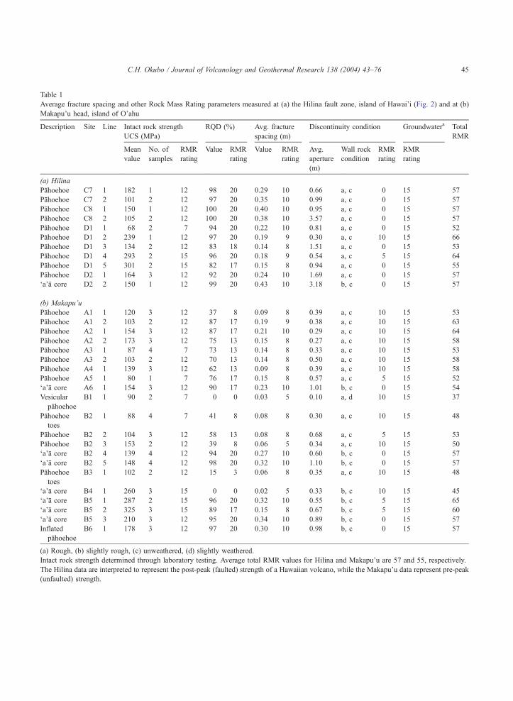
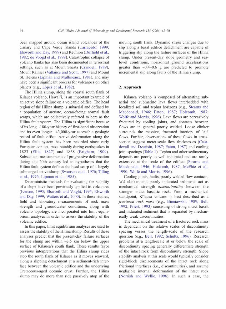
Table 1
Average fracture spacing and other Rock Mass Rating parameters measured at (a) the Hilina fault zone, island of Hawai’i (Fig. 2) and at (b)
Makapu’u head, island of O’ahu
Description Site Line Intact rock strength
UCS (MPa)
RQD (%) Avg. fracture
spacing (m)
Discontinuity condition Groundwatera Total
RMR
Mean
value
No. of
samples
RMR
rating
Value RMR
rating
Value RMR
rating
Avg.
aperture
(m)
Wall rock
condition
RMR
rating
RMR
rating
(a) Hilina
Pahoehoe C7 1 182 1 12 98 20 0.29 10 0.66 a, c 0 15 57
Pahoehoe C7 2 101 2 12 97 20 0.35 10 0.99 a, c 0 15 57
Pahoehoe C8 1 150 1 12 100 20 0.40 10 0.95 a, c 0 15 57
Pahoehoe C8 2 105 2 12 100 20 0.38 10 3.57 a, c 0 15 57
Pahoehoe D1 1 68 2 7 94 20 0.22 10 0.81 a, c 0 15 52
Pahoehoe D1 2 239 1 12 97 20 0.19 9 0.30 a, c 10 15 66
Pahoehoe D1 3 134 2 12 83 18 0.14 8 1.51 a, c 0 15 53
Pahoehoe D1 4 293 2 15 96 20 0.18 9 0.54 a, c 5 15 64
Pahoehoe D1 5 301 2 15 82 17 0.15 8 0.94 a, c 0 15 55
Pahoehoe D2 1 164 3 12 92 20 0.24 10 1.69 a, c 0 15 57
daTa core D2 2 150 1 12 99 20 0.43 10 3.18 b, c 0 15 57
(b) Makapu’u
Pahoehoe A1 1 120 3 12 37 8 0.09 8 0.39 a, c 10 15 53
Pahoehoe A1 2 103 2 12 87 17 0.19 9 0.38 a, c 10 15 63
Pahoehoe A2 1 154 3 12 87 17 0.21 10 0.29 a, c 10 15 64
Pahoehoe A2 2 173 3 12 75 13 0.15 8 0.27 a, c 10 15 58
Pahoehoe A3 1 87 4 7 73 13 0.14 8 0.33 a, c 10 15 53
Pahoehoe A3 2 103 2 12 70 13 0.14 8 0.50 a, c 10 15 58
Pahoehoe A4 1 139 3 12 62 13 0.09 8 0.39 a, c 10 15 58
Pahoehoe A5 1 80 1 7 76 17 0.15 8 0.57 a, c 5 15 52
daTa core A6 1 154 3 12 90 17 0.23 10 1.01 b, c 0 15 54
Vesicular
pahoehoe
B1 1 90 2 7 0 0 0.03 5 0.10 a, d 10 15 37
Pahoehoe
toes
B2 1 88 4 7 41 8 0.08 8 0.30 a, c 10 15 48
Pahoehoe B2 2 104 3 12 58 13 0.08 8 0.68 a, c 5 15 53
Pahoehoe B2 3 153 2 12 39 8 0.06 5 0.34 a, c 10 15 50
daTa core B2 4 139 4 12 94 20 0.27 10 0.60 b, c 0 15 57
daTa core B2 5 148 4 12 98 20 0.32 10 1.10 b, c 0 15 57
Pahoehoe
toes
B3 1 102 2 12 15 3 0.06 8 0.35 a, c 10 15 48
daTa core B4 1 260 3 15 0 0 0.02 5 0.33 b, c 10 15 45
daTa core B5 1 287 2 15 96 20 0.32 10 0.55 b, c 5 15 65
daTa core B5 2 325 3 15 89 17 0.15 8 0.67 b, c 5 15 60
daTa core B5 3 210 3 12 95 20 0.34 10 0.89 b, c 0 15 57
Inflated
pahoehoe
B6 1 178 3 12 97 20 0.30 10 0.98 b, c 0 15 57
(a) Rough, (b) slightly rough, (c) unweathered, (d) slightly weathered.
Intact rock strength determined through laboratory testing. Average total RMR values for Hilina and Makapu’u are 57 and 55, respectively.
The Hilina data are interpreted to represent the post-peak (faulted) strength of a Hawaiian volcano, while the Makapu’u data represent pre-peak
(unfaulted) strength.
C.H. Okubo / Journal of Volcanology and Geothermal Research 138 (2004) 43–76 45

C.H. Okubo / Journal of Volcanology and Geothermal Research 138 (2004) 43–7646
strength of the intact rock is assumed to be much
greater than the strength of the discontinuity, and the
tendency for block translation is directly related to the
frictional strength of the discontinuity and driving
stress (e.g., statics).
At a relative scale where the spacing of constit-
uent discontinuities is much smaller than the length-
scale of the problem, principles of rock mass
mechanics are most applicable (Bieniawski, 1976,
1989; Hoek, 1983). Slope stability analysis at this
scale would typically consider the effective strength
and deformability of the rock mass as a whole, with
the relative contributions of the generally lower
mechanical strength of preexisting discontinuities
interacting with the generally higher mechanical
strength of the intact rock. Consequently, the peak
strength of a fractured rock mass is commonly
controlled by the generally lower strength of
constituent discontinuities. Slope failure (faulting)
within a rock mass commonly involves slip along a
failure plane, as well as internal deformation and slip
along preexisting discontinuities. At this scale, the
tendency for slip is directly related to both the
strength of the failure plane as well as the internal
strength of the rock mass.
Field measurements of discontinuity spacing at
outcrops within the Hilina slump show average
discontinuity spacings of 0.14–0.43 m (Table 1).
These decimeter-scale average discontinuity spac-
ings are 5 orders of magnitude less than the 10s
of kilometers length-scale of the Hilina slump
(Figs. 1, 2). The observed scale of discontinuity
spacing in the field is much smaller than the
Fig. 1. Location of the Hilina slump study area of Fig. 2 and the
Rock Mass Rating collection area on the island of O’ahu.
length-scale of the problem. Accordingly, the
following rock mass mechanics based approach to
analyzing the stability of the Hilina slump is
proposed.
2.1. Stability analysis
Slope failure in a fractured rock mass commonly
occurs by one of four general modes, depending on
the degree of structural control of the failure surface
by preexisting discontinuities (Varnes, 1978; Hoek
and Bray, 1981; Cruden and Varnes, 1996). A
planar failure occurs where a single discontinuity, or
a set of commonly oriented discontinuities, dips in
the direction of slope face. Intersection of these
discontinuities with the slope face promotes sliding
of the overlying rock mass in the down-slope
direction. Such preexisting discontinuities provide
structural control (nucleation sites) for incipient
shear displacements, which can lead to the develop-
ment of a fully yielded failure surface. Similarly,
wedge failure occurs where two preexisting dis-
continuities, or discontinuity sets, intersect within a
slope. In both planar and wedge failure modes, the
rock mass undergoes minimal rotation during lateral
translation along the failure surface. Preexisting
subvertical discontinuities provide structural control
for toppling failure. In this failure mode, the top of
the failed block rotates away from the slope face,
leading opening-mode displacements along disconti-
nuities at the top of the slope during incipient
failure.
Circular failure commonly occurs where preexist-
ing structural control is weak to non-existent at the
length-scale of the slope. Here, a continuous incipient
shear surface is generated dynamically during move-
ment of the failed rock mass. The geometry of the
failure surface generally varies between a shallow arc
and a flat-bottomed arc. Incipient rotation of the slide
is dominated by shear displacements accommodated
along this arc-shaped bcircularQ failure surface (Fig.
3). Displacements along the failure surface at the up-
slope head of the slide are characterized by normal
faulting, with the slide head down-dropped relative to
the original surface. At the toe, or down-slope end of
the slide, shear displacements along the failure surface
are characterized by thrust faulting, with attendant
folding of the surrounding rock mass. Circular failure
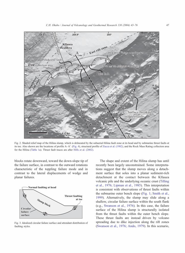
Fig. 2. Shaded relief map of the Hilina slump, which is delineated by the subaerial Hilina fault zone at its head and by submarine thrust faults at
its toe. Also shown are the locations of profile A–AV (Fig. 4), structural profile of Zucca et al. (1982), and the Rock Mass Rating collection area
for the Hilina (Table 1a). Thrust fault traces are after Hills et al. (2002).
C.H. Okubo / Journal of Volcanology and Geothermal Research 138 (2004) 43–76 47
blocks rotate downward, toward the down-slope tip of
the failure surface, in contrast to the outward rotations
characteristic of the toppling failure mode and in
contrast to the lateral displacements of wedge and
planar failures.
CircularCircular
failurefailure
surfacesurface
Circular
failure
surface
Slump block
Normal faulting at head
Thrust faulting
at toe
Fig. 3. Idealized circular failure surface and attendant distribution of
faulting styles.
The shape and extent of the Hilina slump has until
recently been largely unconstrained. Some interpreta-
tions suggest that the slump moves along a detach-
ment surface that soles into a planar sediment-rich
detachment at the contact between the Kılauea
volcanic pile and the underlying oceanic crust (Tilling
et al., 1976; Lipman et al., 1985). This interpretation
is consistent with observations of thrust faults within
the submarine outer bench slope (Fig. 1; Smith et al.,
1999). Alternatively, the slump may slide along a
shallow, circular failure surface within the south flank
(e.g., Swanson et al., 1976). In this case, the failure
surface of the Hilina slump is structurally isolated
from the thrust faults within the outer bench slope.
These thrust faults are instead driven by volcano
spreading due to dike injection along the rift zones
(Swanson et al., 1976; Ando, 1979). In this scenario,
C.H. Okubo / Journal of Volcanology and Geothermal Research 138 (2004) 43–7648
the Hilina slump rides atop of the south flank as it
spreads seaward along a sediment-rich detachment at
the contact between the Kılauea volcanic pile and the
oceanic crust (Swanson et al., 1976; Francis et al.,
1993; Smith et al., 1999).
Recent observations from a multichannel seismic
reflection survey of Kılauea’s submarine south flank
(Morgan et al., 2000, 2003; Hills et al., 2002) have
revealed new insight into the structure of the Hilina
slump. Morgan et al. (2003) identify a candidate
failure surface for the Hilina slump. This surface is 3–
5 km deep and is consistent with the geometry of a
circular failure. The toe of the slide is buried by
onlapping sediments within the submarine mid-slope
basin. Toward the southwest, the toe is exposed, and
the failure surface daylights as a thrust fault, along the
southwest boundary of the western flank of the slump.
This thrust follows the southern boundary of the
western flank through Papa’u ridge, which is revealed
to be a forced fold along the boundary of the failure
surface. Additionally, the outer bench slope thrust
faults are observed to sole into a detachment at the
contact between the base of Kılauea volcanic pile and
the oceanic crust (Morgan et al., 2000; Hills et al.,
2002). The Hilina failure surface does not intersect the
thrusts that daylight in the outer bench, nor does the
Hilina failure surface sole into the basal detachment
(Morgan et al., 2003).
A circular failure character for the Hilina slump is
supported by mechanical considerations of slope
failure for the predicted discontinuity conditions of
the south flank. Kılauea volcano is best described as
a mechanically homogeneous rock mass at the scale
of the Hilina slump. Although stratified by the
distinct products of submarine and subaerial volcan-
ism, as well as intrusive and extrusive rocks, and
attendant density variations, as a whole the edifice of
Kılauea lacks apparent preexisting structural controls
that would promote tens of kilometers-scale planar,
wedge, or toppling failure in the vicinity of the
Hilina slump. Although Kılauea’s eruptive products
are lithologically and morphologically distinct, these
products are predicted to be mechanically homoge-
neous in their strength and deformability at the scale
of the Hilina slump. (This point will be further
explored in a subsequent discussion of rock mass
strength.) Thus, a circular failure geometry can be
reasonably invoked for landslides within the south
flank on the basis of mechanical considerations
alone.
There is also a wealth of subaerial field-based
observations supporting circular failure interpretations
for the Hilina failure surface. Displacements within
the head region of a circular failure are characterized
by maximum subsidence near the head scarp. With the
downward rotation of the head region, the magnitude
of subsidence decreases toward the central region of
the slump. At the Hilina slump, this sense of rotation
would result in tilting of originally horizontal lava
flows so that the flows dip back toward the Hilina
faults. Results of paleomagnetic inclination studies
(Riley et al., 1999) clearly show this sense of
backward rotation of lava flows and ash layers in
the head region of the Hilina slump. The magnitude of
apparent rotation increases with age, consistent with
cumulative rotation due to progressive non-cata-
strophic slope failure for the past ~43,000 years.
These paleomagnetic rotations also suggest that the
failure surface for the Hilina is shallow, within ~5 km
depth (Riley et al., 1999). Lava flow ponding against
the Hilina faults (Swanson et al., 1976) is also
consistent with the backward rotation of the head
region of a circular failure. Additionally, measure-
ments of offsets in N750-year-old lava flows exposed
along the Hilina faults consistently reveal shallow
(~208) slip vector plunges, consistent with a circular
failure surface at shallow depth (Cannon and Burg-
mann, 2001).
Slip along a shallow circular failure surface is also
consistent with the results of long-term trilateration,
leveling, tilt and GPS monitoring of the subaerial head
region of the Hilina slump (Delaney et al., 1993;
Owen et al., 1995, 2000). Model inversions of
deformation associated with the 1975 Kalapana earth-
quake support a shallow failure surface for the Hilina
slump (Cannon et al., 2001). Also, best-fit elastic
models of GPS-derived surface deformation during an
aseismic deformation event on the Hilina slump in
November 2000 are consistent with thrusting along
the toe of a circular failure at ~5 km depth (Cervelli et
al., 2002).
The stability against sliding of a circular failure
surface is commonly assessed using the bmethod of
slicesQ approach (e.g., Duncan, 1996) to descretize the
slide mass. Various methodologies for implementing
this approach have been developed to suit case-
C.H. Okubo / Journal of Volcanology and Geothermal Research 138 (2004) 43–76 49
specific constraints on failure surface geometry (arc
vs. flat bottomed arc) and the relative importance of
specific driving and resisting stresses (e.g., Spencer,
1967; Morgenstern and Price, 1965; Sarma, 1973). In
general, these approaches weigh the magnitude of the
resisting frictional and cohesive strength of potential
failure planes against the resolved shear stress driving
slip along those planes. For example, the tendency for
slope failure by frictional sliding can be assessed in
terms of the Coulomb failure criterion cast in factor of
safety (Fs) form:
Fs ¼P
sPCo4þ rn � rp
� �tan/4
� � ð1Þ
where s is the magnitude of shear stress resolved
along the potential failure surface, Co* is rock mass
cohesion, /* is the friction angle of the rock mass, rn
is the magnitude of the normal stress resolved along
the failure surface, and rp is pore fluid pressure acting
along the failure surface. Both shear and normal stress
magnitudes are derived from the weight of the
overlying rock mass. Optionally, a horizontal stress
due to pseudostatic horizontal ground acceleration can
be incorporated with the resolved shear and normal
stresses acting along the failure plane in order to
evaluate the effect of these forces on the dynamic
stability of the slope.
Factor of safety is the ratio between driving to
resting stress. In Eq. (1), the resolved shear stress acts
to drive slip, while the cohesive and frictional strength
of the failure plane resists slip. Accordingly, slip is
predicted where Fsb1 and incipient slip is predicted
where Fs=1. No slip (stability) is predicted where
FsN1.
The remainder of this paper will detail a rock
mass mechanics based analysis of the geometry and
stability of the failure surface below the Hilina
slump. The program XSTABL (Sharma, 1994) is
used to perform these analyses. XSTABL utilizes
standard force and moment equilibrium methods
(e.g., Bishop, 1955; Janbu, 1954) to find the least
stable circular failure surface for the topology of the
Hilina slump with the rock mass strength parameters
of Kılauea volcano. This approach is iterative and
assumes a circular to arcuate failure surface, the size
and location of which is not strictly determined a
priori. Additionally, horizontal ground accelerations
of various magnitudes, changes in sea level and
topology are simulated in order to investigate the
effects of these events on the stability of the Hilina
slump. In the next section, the outcrop-scale charac-
teristics of Kılauea’s edifice are evaluated through
rock mechanics analyses in order to extract the
strength parameters needed to carry out the method
of slices analyses.
2.2. Rock mass strength of Kılauea
2.2.1. Rock mass rating
The magnitude of stress required to deform a rock
mass is directly related to the strength of the weakest
rock mass component, namely preexisting disconti-
nuities. This is because frictional slip and opening-
mode displacements along discontinuities and fully
yielded fracture surfaces can occur at lower magni-
tudes of resolved driving stress than the magnitudes of
stress required to drive fracture propagation within
intact rock (Hoek, 1983; Schultz, 1996; Hoek and
Brown, 1997). Of course, secondary mineralization
within void spaces may act to heal discontinuities,
necessitating recurrence of fracture propagation and
causing the overall strength of the rock mass to
approach the higher strength of the intact rock or
discontinuity fill. Therefore, a system for evaluating
the strength of a rock mass must account for the
strength of the preexisting discontinuities, as well as
the strength of secondary mineralization (if any)
within these discontinuities and also intact rock
strength.
Relations between the strength of preexisting
discontinuities and overall rock mass strength have
been developed for use in mining and geotechnical
applications. Common rock mass rating schemes,
such as the Rock Mass Rating (RMR) system
(Bieniawski, 1976; 1989) or Geologic Strength Index
(Hoek, 1994; Hoek et al., 1995) rely heavily upon
field-based determinations of specific measurements
of discontinuity strength conditions.
Collection of discontinuity data necessary for
determination of a rock mass’ RMR value is
accomplished through the use of a scanline. In
general, this method involves first stretching a
measuring tape across the outcrop. Then at the points
where the tape intersects a discontinuity, the distance
along the tape is recorded, as well as the conditions,
C.H. Okubo / Journal of Volcanology and Geothermal Research 138 (2004) 43–7650
and optionally orientations, of the traversed disconti-
nuities. The spacing between discontinuities is calcu-
lated by subtraction of consecutive intersection
distances along the measuring tape. The average
discontinuity spacing is consecutively recalculated
with each new measurement. This process is repeated
until the average value for discontinuity spacing
converges, or until the end of the outcrop is reached.
Alternatively, drill core samples may be similarly
analyzed to determine RMR values for otherwise
inaccessible regions of the rock mass (e.g., Deere,
1964; Priest and Hudson, 1976).
Table 2 lists the discontinuity conditions, and their
relative weights, that are used to determine the RMR
value of a rock mass. The frictional strength of
discontinuities is directly assessed through observa-
tions of wall rock roughness, degree of weathering,
and pore fluid pressure. The cohesive strength of the
Table 2
Relative weights of observational and laboratory-determined parameters u
1. Intact rock
strength
Point-load
Index (MPa)
N10 10–4 4–
Uniaxial
compressive
strength,
UCS (MPa)
N250 250–100 10
Rating 15 12 7
2a. RQD (%) 100–90 90–75 75
Rating 20 17 13
2b. Average discontinuity
spacing (m)
N2 2–0.6 0.
Rating 20 15 10
2c. Discontinuity condition Very rough,
discontinuous,
no separation,
unweathered
Rough walls,
separation
b0.1 mm,
slightly
weathered
Sl
se
b1
w
Rating 30 25 20
3. Groundwater Inflow per
10 m tunnel
length (l/min)
None b10 10
Pore fluid
pressure/r1
0 b0.1 0.
General
conditions
Completely
dry
Damp W
Rating 15 10 7
Rating values for each of the five parameters are summed to obtain cumu
discontinuities is evaluated by the degree and charac-
ter of secondary mineralization.
The arithmetic weight of these discontinuity
strengths relative to the overall strength of the rock
mass is determined from meter-scale spacing, as well
as through Rock Quality Designation (RQD), which is
a measure of the centimeter-scale discontinuity
density (Priest and Hudson, 1976). RQD is calculated
as the cumulative length of discontinuity spacings that
are greater than 0.1 m divided by the total length of
the scanline, multiplied by 100. RQD is essentially the
percent of discontinuity spacings that are greater than
0.1 m.
Finally, the unconfined compressive strength
(UCS) of the intact rock is assessed through labo-
ratory testing. At most, intact rock strength contrib-
utes to only 15% of the total rock mass strength, as
evaluated by RMR (Bieniawski, 1989). In contrast,
sed to calculate RMR
2 2–1
0–50 50–25 25–5 5–1 b1
4 2 1 0
–50 50–25 b25
8 3
6–0.2 0.2–0.06 b0.06
8 5
ightly rough,
paration
mm, highly
eathered
Slickensides or
Gouge b5 mm
thick or separation
1–5 mm, continuous
Soft gouge N5 mm
thick or Separation
N5 mm, continuous,
decomposed
rock wall
10 0
–25 25–125 N125
1–0.2 0.2–0.5 N0.5
et Dripping Flowing
4 0
lative RMR value.
C.H. Okubo / Journal of Volcanology and Geothermal Research 138 (2004) 43–76 51
discontinuity strength can represent up to 65% of the
total rock mass strength.
Individual ratings for each set of parameters are
summed to arrive at a RMR value for the rock mass.
Additional corrections for discontinuity orientations
can also be applied (Bieniawski, 1989). An RMR
value of 100 corresponds to a rock mass with strength
approaching that of intact rock, while lower values of
RMR correspond to lower rock mass strengths.
Ideally, the average RMR value of three orthogonal
scanlines, or core, is used to establish a three-
dimensional value of RMR for the outcrop. Within a
rock mass that contains subsections of significantly
different RMR, such as a fault zone through blocky
but undisturbed rock, individual values for each
distinct RMR region can be area- or volume-averaged
to arrive at an overall RMR value for the rock mass.
In cases where drill core samples are unavailable
and scanline surveys are not possible, values of RMR
can be calculated from crustal density and P-wave
velocity structure. This method as discussed below is
based on established relations between RMR, defor-
mation modulus of the rock mass and P-wave velocity.
Rock mass density, q*, and P-wave velocity, Vp,
are related to the dynamic deformation modulus of a
rock mass, Ed* (in Pa), through:
Ed4 ¼ q4V 2p
1� 2m4ð Þ 1þ m4ð Þ1þ m4ð Þ
where m* is Poisson’s ratio for the rock mass (Jaeger
and Cook, 1979). Ed* is analogous to the dynamic
Young’s modulus for intact rock (International Society
for Rock Mechanics, 1975).
Through in situ testing and back-analyses, the
following relations to RMR have been developed for
the static deformation modulus of a rock mass, Es* (in
GPa). For values of RMR between 50 and 100:
Es4 ¼ 2RMR� 100
and for values of RMR less than 50:
Es4 ¼ 10 RMR�10ð Þ=40
(Bieniawski, 1978; Hoek and Brown, 1988). Solving
for RMR yields:
RMR ¼ 1
2Es4
�þ 50
�
for values of RMR between 50 and 100 and:
RMR ¼ 40logEs4ð Þ þ 10
for values of RMR less than 50.
Laboratory experiments and in situ testing of
basaltic rock masses suggest an Ed*/Es* ratio of
approximately 2 (Cheng and Johnson, 1981; Gud-
mundsson, 1988; Forslund and Gudmundsson, 1991).
Thus, substituting Ed* for Es* in the above equations
yields relations for RMR based on the dynamic
deformation modulus of the rock mass. For values
of RMR between 50 and 100:
RMR ¼ 1
4Ed4
�þ 50
�
and for values of RMR less than 50:
RMR ¼ 40log1
2Ed4
�þ 10
�
Accordingly, the effective RMR of a rock mass can be
estimated from Vp through:
RMR ¼ 1
4q4V 2
p
1� 2m4ð Þ 1þ m4ð Þ1� 106� �
1� m4ð Þ
!þ 50
ð2Þ
for values of RMR between 50 and 100 and through:
RMR ¼ 40log1
2q4V 2
p
1� 2m4ð Þ 1þ m4ð Þ1� 106� �
1� m4ð Þ
!þ 10
ð3Þ
for values of RMR less than 50. Here, Vp is P-wave
velocity in m/s and q* is rock mass density in kg/m3.
Eq. (2) is valid only when the calculated value of
RMR is greater than 50. Similarly, Eq. (3) is strictly
valid for resulting RMR values less than 50. If a value
of RMR is calculated outside of the range of the
respective equation, then the alternate equation must
be used.
For sufficiently large values of density and P-wave
velocity, Eq. (2) will return values of RMR greater
than 100, for which RMR is undefined. The limiting
RMR value of 100 corresponds to rock mass strength
and deformability approaching that of the intact rock.

C.H. Okubo / Journal of Volcanology and Geothermal Research 138 (2004) 43–7652
Therefore, a value of RMR greater than 100, as
calculated from Eq. (2), should suggest that intact
rock behavior is more appropriate than RMR-derived
properties for the problem at hand. Essentially, Eq. (2)
can be used to define the limits at which rock mass
strength analysis should be replaced by intact rock
strength criteria for a given set of P-wave velocity,
density and Poisson’s ratio values.
Surface exposures of rock mass structure are
abundant along the south flank of Kılauea, facilitat-
ing determination of RMR for the uppermost
surface of the edifice. The internal RMR structure
of Kılauea however, is more elusive. Deep drill core
data are unavailable for the south flank of Kılauea
in and around the Hilina slump. Deep mine shafts,
or other exploration tunnels, are also non-existent in
this area.
At present, the deep RMR structure of the south
flank of Kılauea must be determined from inter-
pretations of the volcano’s density and P-wave
velocity structure. Zucca et al. (1982) applied
geophysical analyses of seismic and gravity data
to infer a density and P-wave velocity structure of
the south flank of Kılauea. These data are the
most recent available that relate geologic units, P-
wave velocity and density structure in sufficient
detail at the scale of the Hilina slump. Accord-
ingly, the RMR structure of the south flank can be
Table 3
Density, P-wave and burial depth values for south flank Kılauea geologic u
(1) and corresponding values of /* and Co*
Geologic unit P-wave velocity
(km/s)
Density (kg/m3) Burial depth
(m)
Min Max Min Max Min Max
Unsaturated 1800 2500 2400 2800 0 900
Subaerial flows
and clastic
deposits
1800 2500 2400 2800 0 900
Saturated 2800 3200 2400 2800 0 2650
Subaerial flows
and clastic
deposits
2800 3200 2400 2800 0 2650
Submarine 4600 5400 2500 2900 2620 6848
Pillow basalt 4600 5400 2500 2900 2620 6848
Intrusive 6500 7300 2700 3100 350 11,958
Complex 6500 7300 2700 3100 350 11,958
Oceanic crust 6900 7100 2700 3100 1085 16,958
6900 7100 2700 3100 1085 16,958
estimated from these results by applying Eqs. (2)
and (3).
The structural profile of Zucca et al. (1982)
extends from the northeast rift zone of Mauna
Loa, across the southwest rift zone and along the
south flank of Kılauea. Based on the predicted
distribution of density and P-wave velocities,
Zucca et al. (1982) divided the profile into discrete
geologic units that they interpreted as subaerial
flows and clastic deposits, submarine pillow
basalts, intrusive complex, oceanic crust, and upper
mantle.
In order to account for variations in rock mass
strength due to pore fluid pressure, the subaerial flows
and clastic deposits unit is here broken into saturated
and unsaturated sections. This division is defined by a
phreatic surface that is based on the self-potential
results of Jackson and Kauahikaua (1987) and is
broadly consistent with other groundwater models
(e.g., Scholl et al., 1996) at the scale of the Hilina
slump.
Minimum and maximum values of RMR are
calculated through Eqs. (2) and (3) for each geologic
unit based on the ranges of density and P-wave
velocities reported by Zucca et al. (1982) and are
listed in Table 3. The oceanic crust is found to
correspond to a value of RMR of approximately 80
over the range of density and P-wave velocities
nits from Zucca et al. (1982), with ranges of RMR calculated by Eq.
m i UCS (MPa) RMR /* (8) Co* (MPa)
Min Max Min Max Min Max Min Max
15 30 150 350 52 57.5 57.6 1.11 1.24
15 30 150 350 53 57.5 57.6 1.18 1.33
15 30 150 350 54 57.5 57.9 1.24 1.40
15 30 150 350 55 57.5 57.9 1.30 1.47
15 30 150 350 62 58.9 58.6 1.81 2.05
15 30 150 350 66 58.7 58.5 2.21 2.52
15 30 150 350 76 57.7 59.0 4.82 5.59
15 30 150 350 81 57.7 58.7 4.85 5.63
15 30 150 350 79 57.9 59.4 4.82 5.59
15 30 150 350 79 57.9 59.4 4.85 5.63
C.H. Okubo / Journal of Volcanology and Geothermal Research 138 (2004) 43–76 53
reported by Zucca et al. (1982). The intrusive complex
is found to have the highest values of RMR for the
entire volcanic edifice, at 76–81. The submarine
pillow basalt unit corresponds to lower RMR values
of 62–66. Density and P-wave velocities within the
saturated portion of the subaerial flows and clastic
deposits unit correspond to an RMR range of 54–55.
The unsaturated portion (i.e., above the water table)
has calculated RMR values of 52–53. These RMR
values represent the cumulative effective strength of
discontinuities, intact basaltic rock and indurated
clastic sediment (if any) comprising each geologic
unit.
These results show that calculated RMR values
vary at most by a value of 5 over the range of density
and P-wave velocities reported by Zucca et al. (1982).
Uncertainties in RMR measurements made at the
outcrop are typically F15 (e.g., Bieniawski, 1978,
Schultz, 1996). Therefore, the uncertainty in the
model Kılauea values are well within accepted
operational uncertainties of RMR.
The range of RMR values calculated for the
unsaturated subaerial flows and clastic deposits unit
are next tested against field-based determinations of
RMR for this unit (currently the only unit for
which this can be done). Field observations of
discontinuity spacing and condition were obtained
using the procedure outlined above for 11 stations
along the south flank of Kılauea, in proximity to
the faults of the Hilina system (Fig. 2). Table 1a
lists the average discontinuity spacings for each
scanline. At each scanline station, measurements of
fracture spacing were obtained until the values of
average fracture spacing converged. Values of
average fracture spacing that did not converge
before the scanline reached the end of the outcrop
were not used. In this way, the necessary length of
the scanline is dictated by the average fracture
spacing of the rock mass (and calculated dynam-
ically based on the cumulative results of the data
collection), rather than being limited by an
arbitrary maximum length. Systematic fracture
spacings at scales larger than the 10s of meters
scale of the scanlines are not observed in the field.
Therefore, the length of the scanline is necessarily
sufficient to adequately characterize the average
fracture spacing of the larger rock mass at each
station.
The field area lies within the rain shadow of the
summit of Kılauea and is therefore arid and lacks
active groundwater seeps. Accordingly, groundwater
condition at all sites is observed to be completely dry,
corresponding to an RMR rating of 15. Lava flow
types encountered are ’a’a, inflated pahoehoe and
pahoehoe toe complexes, with no clastic layers
encountered. These field measurements yield total
RMR values that range from 52 to 66. As these RMR
measurements were obtained in proximity to fault
scarps, these values may reflect the post-peak
(faulted) strength of the rock mass within the
unsaturated subaerial flows and clastic deposits unit.
Pre-peak (unfaulted) values of RMR for a typical
Hawaiian volcano are calculated from observations of
rock mass structure exposed at Makapu’u head, on
Ko’olau volcano (island of O’ahu; Fig. 1). Outcrops at
this site have been exposed through fluvial erosion
and back wasting of coastal headlands. As with the
Hilina observations, lava flow types encountered are
’a’a, inflated pahoehoe and pahoehoe toe complexes,
with no clastic layers encountered. Table 1b lists the
RMR measurements made at Makapu’u.
Although the post-peak Hilina data show slightly
lower values of RMR than the pre-peak Makapu’u
data, the difference between pre-peak and post-peak
values is not significant. This suggests that incremen-
tal fault slip at the scale of the Hilina within a
Hawaiian volcano may not significantly reduce the
strength of the surrounding rock mass away from the
fault. This would imply that subsequent faulting might
not necessarily follow established fault planes, but
rather propagate along failure paths that are optimally
oriented for slip under the local driving stresses.
Comparison of Tables 1 and 3 show that the P-
wave and density derived values of RMR for the
unsaturated subaerial flows and clastic deposits unit
are generally consistent with the pre-peak RMR data
obtained at Makapu’u and with the post-peak RMR
data obtained at Hilina. The predicted values of RMR
are generally in line with near surface observations of
RMR. Thus, based on the P-wave and density derived
values of RMR, the mechanical strength of Kılauea’s
south flank can now be determined.
2.2.2. Rock mass strength
Values of RMR can be related to rock mass strength
parameters, such as friction angle and shear modulus,
C.H. Okubo / Journal of Volcanology and Geothermal Research 138 (2004) 43–7654
through sets of empirical equations (e.g., Hoek, 1983;
Hoek and Brown, 1997). These equations are devel-
oped from back-analysis recovery of peak stress and
pre-failure values of RMR at mines, foundations, and
natural and engineered slopes (Hoek and Brown, 1980,
1997; Hoek, 1983), as well as from large-scale in situ
testing of stress–strain behavior (Bieniawski, 1978).
For this study, values of rock mass cohesive
strength, Co*, and internal friction angle, /*, must
be determined in order to assess the stability of a slope
using the method of slices. The cohesive strength of a
rock mass is given by:
Co4 ¼ rc
ffiffiffiffiffiffiffiffiffiffiffiffiffiffiffiffiffiffim2 þ 16s
p� m
4
!
�ffiffiffiffiffiffiffiffiffiffiffiffiffiffiffiffiffiffiffiffiffiffiffiffiffiffiffiffiffiffiffiffiffiffiffiffiffiffiffiffiffiffiffiffiffiffiffiffiffiffiffiffiffiffiffiffiffiffiffiffiffiffir2c þ
16mrc
ð4 ffiffis
p � mþffiffiffiffiffiffiffiffiffiffiffiffiffiffiffiffiffiffim2 þ 16s
pÞ2
sð4Þ
where rc is the unconfined compressive strength of
the intact rock (Hoek, 1983). The parameters m and s
are empirical rock mass strength constants (Hoek and
Brown, 1997):
m ¼ mieRMR� 100
28
��
s ¼ eRMR� 100
9
��
These dimensionless parameters relate values of RMR
to rock mass strength and thereby reflect discontinuity
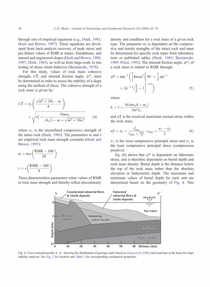
Fig. 4. Cross-sectional profile A–AV showing the distribution of geologic u
stability analyses. See Fig. 2 for location and Table 3 for corresponding m
density and condition for a rock mass of a given rock
type. The parameter mi is dependent on the compres-
sive and tensile strengths of the intact rock and must
be determined for specific rock types from laboratory
tests or published tables (Hoek, 1983; Bieniawski,
1989; Priest, 1993). The internal friction angle, /*, of
a rock mass is related to RMR through:
/4 ¼ tan�1
��4hcos2
308þ 1
3sin�1
� h�1:5� ��
� 1
��0:5�ð5Þ
where
h ¼ 1þ 16 mrn4þ srcð Þ3m2rc
and rn* is the resolved maximum normal stress within
the rock mass:
rn4 ¼ r3 þs2max
smax þ mrc
8
; smax ¼r1 � r2
2ð6Þ
r1 is the most compressive principal stress and r3 is
the least compressive principal stress (compression
positive).
Eq. (6) shows that /* is dependent on lithostatic
stress, and is therefore dependent on burial depth and
rock mass density. Burial depth is the distance below
the top of the rock mass rather than the absolute
elevation or bathymetric depth. The maximum and
minimum values of burial depth for each unit are
determined based on the geometry of Fig. 4. This
nits based on Zucca et al. (1982) and used here at the basis for slope
echanical properties.
C.H. Okubo / Journal of Volcanology and Geothermal Research 138 (2004) 43–76 55
range of burial depths and the ranges of rock mass
densities from Zucca et al. (1982) are used to calculate
/*.
The range of cohesion and friction for each
geologic unit is calculated through Eqs. (4) and (5)
based on the model Kılauea values of RMR. Mini-
mum and maximum values of mi of 15 and 30, typical
for basalt (e.g., Hoek, 1983), are used to bracket
expected natural variations in mi. The unconfined
compressive strength of the intact rock is bracketed
for typical values for basalt between 150 and 350 MPa
(e.g., Table 1; Lama and Vutukuri, 1978).
Table 3 shows ranges of Co* and /* calculated by
Eqs. (4) and (5), respectively, based on the values of
RMR corresponding to the minimum and maximum
P-wave velocity and density values reported by Zucca
et al. (1982). Within these ranges of rock mass
parameters, /* varies at most by 1.58 (within the
oceanic crust) and Co* varies at most by 0.81 MPa
(within the intrusive complex). These ranges of Co*
and /* are consistent with commonly reported values
of minimally weathered fractured rock masses of
varying composition (e.g., Hoek, 1983).
Values of RMR determined from Eqs. (2) and (3),
as well as values determined from field observations,
yield internal friction angles of 57.5–59.48 for units
within the Hilina slump (e.g., Table 3). These friction
angles are larger than values typically reported for
samples of intact basalt (e.g., 34–468; U.S. DOE,
1988). Clay alteration of the intact rock can result in
even smaller friction angles (e.g., 13–408; Watters and
Delahaut, 1995).
Values of friction comparable to the results reported
Table 3 are consistent with previously reported values
for igneous rock masses (Schultz, 1995, 1996; Bye and
Bell, 2001). Larger values of apparent friction within
the rock mass can be attributed to interlocking and
lateral confinement of key blocks of intact rock (e.g.,
block theory; Goodman and Shi, 1985), which
effectively increase the roughness of the failure surface
(e.g., Barton, 1976). Additionally, deep core retrieved
by the Hawaii Scientific Drilling Project shows
negligible argillic alteration within the central older
rock mass of neighboring Mauna Kea volcano (Garcia,
1996), suggesting minimal frictional strength loss due
to argillic alteration at distance from the rift zones at
Kılauea. The relatively high values of /* reported in
Table 3 are regarded as reasonable for Kılauea given
these considerations, as well as observations of near
vertical to overhanging crater walls that have been
exposed due to stoping (e.g., Okubo and Martel, 1998)
in the unsaturated subaerial flows and clastic deposits
unit.
The computed minimum and maximum rock mass
strength values (Table 3) are used to define two
mechanical strength profiles for the south flank of
Kılauea. The minimum strength values for each
geologic unit are used to define a bweakQ strength
profile, and the maximum values are used to define a
bstrongQ strength profile. In this way, the effects of
uncertainties in rock mass strength can be monitored
by separately modeling both the strong and weak
strength profiles in the slope stability analyses.
2.3. Model Setup
The topography and bathymetry of the south flank
of Kılauea used in this slope stability analysis is
extracted from the 3-second resolution digital terrain
model of Smith and Duennebier (personal communi-
cation, 2001). The subaerial sections of the model are
based on the U.S. Geological Survey’s 1:250,000
scale digital elevation model for the island of Hawai’i.
Bathymetry is based on 3-second resolution Sea-
BEAM, sparse hydrographic bathymetry, and variable
resolution GEODAS trackline depths.
For this study, an 80-km-long topologic profile is
constructed along the south flank of Kılauea volcano
(Fig. 2). The profile begins on Kılauea’s east rift zone,
cuts across the Hilina fault system, and extends 60 km
off shore. This profile is sub-parallel with the profile
of Zucca et al. (1982), which is located approximately
10 km to the southwest. The geologic and mechanical
structure of the south flank, derived from Zucca et al.
(1982), is visually fitted to this topologic profile.
Control points used for this fit are the location of the
intrusives of Kılauea’s rift zone, the present-day coast
and the generalized topology of Zucca et al.’s profile.
The resulting model profile encompasses a series
of ocean-facing faults of the Hilina system (Fig. 4).
The northern most Hilina faults of Poliokeawe and
Holei together have a cumulative geologic offset of
approximately 420 m toward the south. The down-
dropped block south of Holei forms a broad coastal
plain. Within this plain is the Kealakomo normal fault
with approximately 60 m offset toward the south. The

C.H. Okubo / Journal of Volcanology and Geothermal Research 138 (2004) 43–7656
profile then crosses the coastline and intersects an
unnamed submarine fault-like step at approximately
30 m depth. A flat-floored topographic depression,
termed the mid-slope basin by Hills et al. (2002); is
encountered at 2.3 km depth, adjacent to a topo-
graphic rise termed the mid-slope bench by Hills et al.
(2002). The profile then traverses the outer bench
slope, then onto the debris apron surrounding the
edifice (e.g., Leslie et al., 2002).
The present-day stability of the Hilina slump is
modeled under static conditions, as well as under
pseudostatic horizontal ground accelerations
(dynamic loads due to earthquakes or explosive
volcanic eruptions) of 0.1–1.0 g, for both weak and
strong strength profiles. The horizontal accelerations
act along the plane of the model profile in the out-of-
slope direction and are constant with depth. Inves-
tigating the dynamic stability of the Hilina slump is
important because the area is predicted to have a
10% chance of experiencing horizontal ground
accelerations exceeding 2 g within 50 years (Klein
et al., 2001). Further, Kılauea has experienced
several historic episodes of explosive eruption (e.g.,
Decker and Christiansen, 1984; Mastin, 1997). The
effects of changes in sea level on the stability of the
Hilina slump are also tested. Numerous submerged
and emerged coastal terraces and deposits throughout
Hawai’i (Coulbourn et al., 1974; Ku et al., 1974;
Stearns and Easton, 1977; Stearns, 1978) and the
Pacific (Sprigg, 1979; Carter et al., 1986; Gibb,
1986; Eisenhauer et al., 1993) have been interpreted
as evidence of past high and low stands of the sea.
High stands of the sea have been interpreted at more
than 360 m above present-day mean sea level
(MSL), and low stands have been proposed at more
than 1000 m below present-day MSL (Stearns,
1978).
Variations in sea level have the potential to effect
the distribution of saturated and unsaturated regions
within a coastal rock mass. Increases in pore fluid
pressure (with increasing fluid saturation) have been
shown to reduce the strength of rock masses by
decreasing the effective confining stress and thereby
decreasing frictional strength of block to block
contacts (e.g., Brace and Martin, 1968; Lade and de
Boer, 1997). In order to evaluate the stability of the
Hilina under sea-level magnitudes that are bracketed
by observations, the effect of a hypothetical sea level
at 300 and 1000 m below present-day MSL on the
stability of the Hilina slump is evaluated. Further, the
effect of a 300-m-high stand of the sea is also
modeled. In these three cases, the minimum elevation
of the water table is set to the hypothetical sea level,
and the distribution of the water table is modeled after
Jackson and Kauahikaua (1987).
Further, the stability effects of loading the head
region of the Hilina slump by lava flow emplacement
are evaluated. Future lava flow emplacement on the
head region of the slump is simulated by raising the
elevation of the unsaturated subaerial flows and clastic
deposits unit to a uniform elevation of 500 m between
the top of the Holei fault scarp and the present-day
coastline.
For all scenarios, pore fluid pressure within the
rock mass is determined relative to the prescribed
phreatic surface. Pore pressure increases linearly
with depth below the phreatic surface throughout
the entire subjacent rock mass. Additionally, the
level of the phreatic surface at the coastline is
defined to be mean sea level. This increase in pore
pressure with depth is uniform across discontinuities
(slip surfaces and unit interfaces). An increase in
pore pressure due to enhanced periods of rainfall
may have triggered an aseismic slip event on along
the Hilina fault system (Cervelli et al., 2002).
Although such transient variations in pore pressure
may be influence Hilina stability, these variations
cannot be evaluated by the current analysis. Further,
variability in pore pressure due to slip-induced
stress change and variability in pore pressure due
to dynamic stresses from applied horizontal accel-
erations (e.g., Skempton, 1954; Law and Holtz,
1978) are not evaluated.
In all test cases, the slope stability analysis
techniques of Janbu’s simplified method (Janbu,
1954) and Bishop’s modified method (Bishop, 1955)
are independently used to assess the stability of each
strength model. Bishop’s modified method determines
vertical force equilibrium and moment equilibrium
and is commonly used for cases of arc-shaped failure
surfaces. Janbu’s simplified method is a force
equilibrium approach that is commonly used for arc-
to flat-bottomed-arc-shaped failure surfaces. These
approaches are capable of evaluating the contributions
of static pore fluid pressure and pseudostatic ground
accelerations on the stability of potential circular
C.H. Okubo / Journal of Volcanology and Geothermal Research 138 (2004) 43–76 57
failure surfaces within a given slope of a prescribed
topographic profile and rock mass strength. Using
these two different methods, the factor of safety, as
well as the least stable surface geometry, is deter-
mined for each test case. Each analysis technique
satisfies selected principals of statics, essentially force
and moment equilibrium for the failure mass.
Janbu’s simplified method (Janbu, 1954) uses the
method of slices to discretize a failure mass into
vertical slices and to calculate a factor of safety for the
entire slide. This method assumes that interslice shear
forces are zero and that only horizontal interslice
normal forces are non-zero. The governing equations
for this analysis satisfy force equilibrium for each
slice and horizontal force equilibrium for the entire
slide. Moment equilibrium of the failure slide is
neglected.
Bishop’s modified method (Bishop, 1955) also
uses the method of slices to calculate the factor of
safety for the slump. Similar to the Janbu method, this
method assumes interslice shear forces are zero and
that only horizontal normal interslice forces are non-
zero. This method satisfies vertical force equilibrium
for each slice and moment equilibrium about the
center of curvature of the circular failure surface.
Limit equilibrium analyses are based solely on
material strength (not deformability) and thus can
only determine the static stability of the slump. If
Fs=1, then the sump is in incipient slip. If Fsb1, then
the slump is very unstable and likely to slip. As soon
as slip occurs, other methods (e.g., finite element
models) must be used to predict material deformation.
Further, since material deformability is not evaluated
in the limit equilibrium analysis, local stress concen-
trations due to slope topology do not factor into the
results.
In the Hilina stability analyses, each potential
failure surface is automatically generated in XSTABL
based on a specified fault bterminationQ zone between5 and 15 km and a fault binitiationQ zone between 20
and 70 km along the model profile. Although the
terms binitiation’ and bterminationQ are suggestive of afailure surface propagation process, these terms in fact
refer to the method by which the trial surfaces are
automatically generated in XSTABL. The initiation
zone is separated into 50 evenly spaced segments, and
the middle of each segment is used to define 50 trial
failure surfaces through the rock mass. These failure
surfaces are generated such that they intersect the top
of the rock mass within the termination zone. Thus,
2500 trial failure surfaces are generated for each
model run. The lowest magnitude of Fs and its
corresponding failure surface geometry is then
recorded and plotted. In all cases, The Janbu analyses
are not confined to purely circular failure geometries,
but are free to determine the least stable failure
geometry based on the software-generated trial
surfaces.
The apparent along-strike asymmetry of the Hilina
slump (Smith et al., 1999; Hills et al., 2002; Morgan
et al., 2003) may bring into question the reliability of
2D analyses, as used here, for understanding a fully
3D system. Computational 3D models of circular
failure analysis have been developed based on
expansion of the Bishop method (Hungr, 1987). 3D
distinct element models are also being implemented
(Lorig et al., 1991), and finite element models
(Duncan, 1992) may also be used for 3D slope
analysis. Currently, however, 2D analyses are the
standard for circular failure analysis due to their ease
of experimental setup (see references in Norrish and
Wyllie, 1996). Factors of safety calculated by 2D
methods are generally lower than those calculated by
3D analyses, for the least stable 2D section along the
same 3D slide mass under identical conditions
(Cavounidis, 1987; Hungr et al., 1989; Duncan,
1996). 2D analyses generally neglect anti-plane stress.
Normal stresses acting perpendicular to the 2D section
in the 3D case would tend to enhance the internal
(frictional) strength of the slide mass, impeding
internal deformation and promoting stability. There-
fore, factors of safety derived from 2D analyses are
generally considered to be conservative (Duncan,
1996; Norrish and Wyllie, 1996) and are thereby
legitimate for the purpose of this paper.
3. Results
Stability is assessed with both the Bishop and
Janbu methods for zero horizontal ground acceleration
(static stability) and at accelerations of 0.1–10 g. In
both weak and strong cases, the Janbu-predicted
factors of safety are within 5% of the Bishop-
predicted factors of safety. This similarity in the
results of these two methods is also characteristic of
C.H. Okubo / Journal of Volcanology and Geothermal Research 138 (2004) 43–7658
other slope stability analyses (Duncan and Wright,
1980), and suggests that the stability predictions are
not significantly biased by the method of analysis
used. Therefore, for clarity, only the results of the
Bishop analyses are presented.
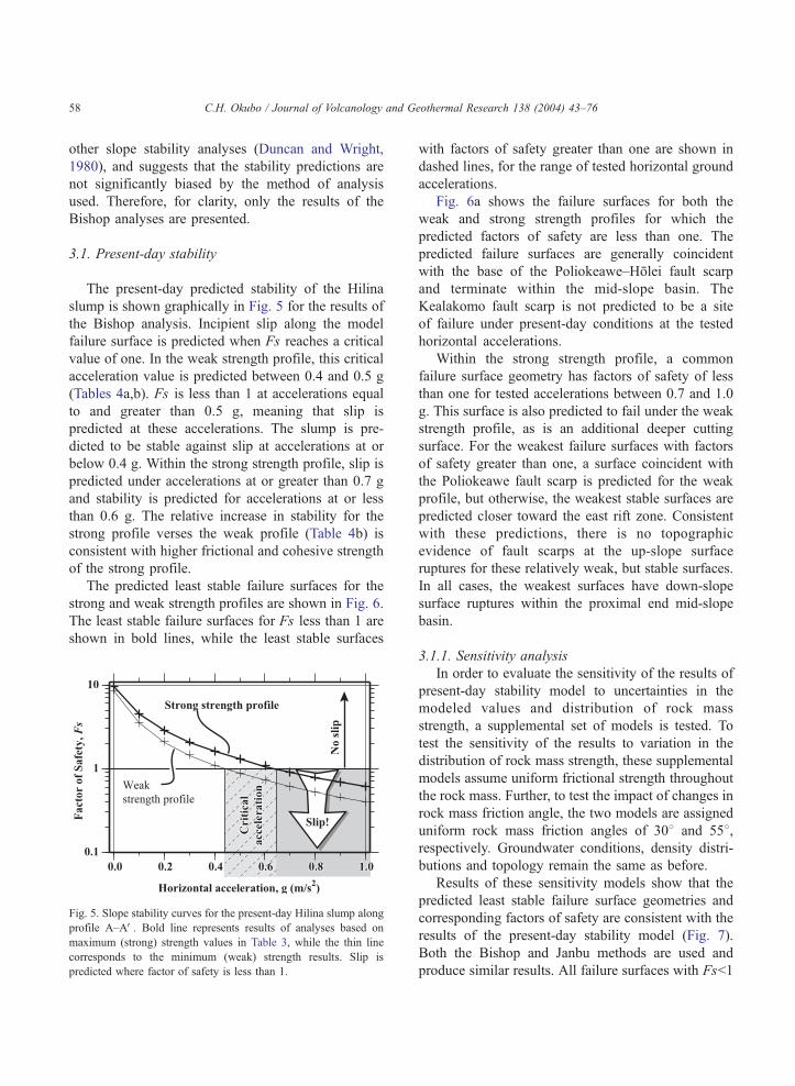
3.1. Present-day stability
The present-day predicted stability of the Hilina
slump is shown graphically in Fig. 5 for the results of
the Bishop analysis. Incipient slip along the model
failure surface is predicted when Fs reaches a critical
value of one. In the weak strength profile, this critical
acceleration value is predicted between 0.4 and 0.5 g
(Tables 4a,b). Fs is less than 1 at accelerations equal
to and greater than 0.5 g, meaning that slip is
predicted at these accelerations. The slump is pre-
dicted to be stable against slip at accelerations at or
below 0.4 g. Within the strong strength profile, slip is
predicted under accelerations at or greater than 0.7 g
and stability is predicted for accelerations at or less
than 0.6 g. The relative increase in stability for the
strong profile verses the weak profile (Table 4b) is
consistent with higher frictional and cohesive strength
of the strong profile.
The predicted least stable failure surfaces for the
strong and weak strength profiles are shown in Fig. 6.
The least stable failure surfaces for Fs less than 1 are
shown in bold lines, while the least stable surfaces
Fig. 5. Slope stability curves for the present-day Hilina slump along
profile A–AV. Bold line represents results of analyses based on
maximum (strong) strength values in Table 3, while the thin line
corresponds to the minimum (weak) strength results. Slip is
predicted where factor of safety is less than 1.
with factors of safety greater than one are shown in
dashed lines, for the range of tested horizontal ground
accelerations.
Fig. 6a shows the failure surfaces for both the
weak and strong strength profiles for which the
predicted factors of safety are less than one. The
predicted failure surfaces are generally coincident
with the base of the Poliokeawe–Holei fault scarp
and terminate within the mid-slope basin. The
Kealakomo fault scarp is not predicted to be a site
of failure under present-day conditions at the tested
horizontal accelerations.
Within the strong strength profile, a common
failure surface geometry has factors of safety of less
than one for tested accelerations between 0.7 and 1.0
g. This surface is also predicted to fail under the weak
strength profile, as is an additional deeper cutting
surface. For the weakest failure surfaces with factors
of safety greater than one, a surface coincident with
the Poliokeawe fault scarp is predicted for the weak
profile, but otherwise, the weakest stable surfaces are
predicted closer toward the east rift zone. Consistent
with these predictions, there is no topographic
evidence of fault scarps at the up-slope surface
ruptures for these relatively weak, but stable surfaces.
In all cases, the weakest surfaces have down-slope
surface ruptures within the proximal end mid-slope
basin.
3.1.1. Sensitivity analysis
In order to evaluate the sensitivity of the results of
present-day stability model to uncertainties in the
modeled values and distribution of rock mass
strength, a supplemental set of models is tested. To
test the sensitivity of the results to variation in the
distribution of rock mass strength, these supplemental
models assume uniform frictional strength throughout
the rock mass. Further, to test the impact of changes in
rock mass friction angle, the two models are assigned
uniform rock mass friction angles of 308 and 558,respectively. Groundwater conditions, density distri-
butions and topology remain the same as before.
Results of these sensitivity models show that the
predicted least stable failure surface geometries and
corresponding factors of safety are consistent with the
results of the present-day stability model (Fig. 7).
Both the Bishop and Janbu methods are used and
produce similar results. All failure surfaces with Fsb1
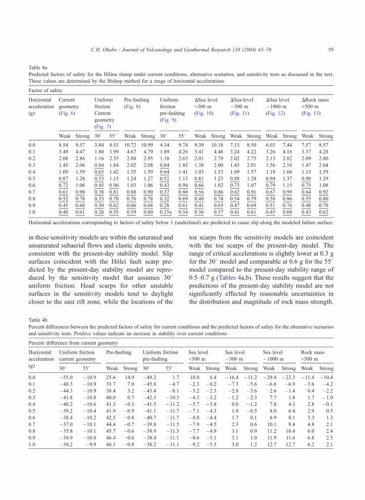
Table 4a
Predicted factors of safety for the Hilina slump under current conditions, alternative scenarios, and sensitivity tests as discussed in the text.
These values are determined by the Bishop method for a range of horizontal accelerations
Factor of safety
Horizontal
acceleration
(g)
Current
geometry
(Fig. 6)
Uniform
friction
Current
geometry
(Fig. 7)
Pre-faulting
(Fig. 8)
Uniform
friction
pre-faulting
(Fig. 9)
DSea level
+300 m
(Fig. 10)
DSea-level
�300 m
(Fig. 11)
DSea level
�1000 m
(Fig. 12)
DRock mass
+500 m
(Fig. 13)
Weak Strong 308 558 Weak Strong 308 558 Weak Strong Weak Strong Weak Strong Weak Strong
0.0 8.54 9.57 3.84 8.53 10.72 10.99 4.34 9.74 9.39 10.18 7.13 8.50 6.03 7.44 7.57 8.57
0.1 3.49 4.47 1.80 3.99 4.67 4.79 1.89 4.26 3.41 4.46 3.24 4.22 3.26 4.16 3.37 4.28
0.2 2.08 2.86 1.16 2.55 2.88 2.95 1.18 2.63 2.01 2.79 2.02 2.75 2.13 2.82 2.09 2.80
0.3 1.45 2.06 0.84 1.84 2.02 2.08 0.84 1.85 1.38 2.00 1.43 2.01 1.56 2.10 1.47 2.04
0.4 1.09 1.59 0.65 1.42 1.55 1.59 0.64 1.41 1.03 1.53 1.09 1.57 1.18 1.66 1.13 1.59
0.5 0.87 1.28 0.53 1.15 1.24 1.27 0.52 1.13 0.81 1.23 0.88 1.28 0.94 1.37 0.90 1.29
0.6 0.72 1.06 0.45 0.96 1.03 1.06 0.43 0.94 0.66 1.02 0.73 1.07 0.79 1.15 0.75 1.08
0.7 0.61 0.90 0.38 0.81 0.88 0.90 0.37 0.80 0.56 0.86 0.62 0.91 0.67 0.99 0.64 0.92
0.8 0.52 0.78 0.33 0.70 0.76 0.78 0.32 0.69 0.48 0.74 0.54 0.79 0.58 0.86 0.55 0.80
0.9 0.45 0.68 0.30 0.62 0.66 0.68 0.28 0.61 0.41 0.65 0.47 0.69 0.51 0.76 0.48 0.70
1.0 0.40 0.61 0.26 0.55 0.59 0.60 0.25x 0.54 0.36 0.57 0.41 0.61 0.45 0.68 0.43 0.62
Horizontal accelerations corresponding to factors of safety below 1 (underlined) are predicted to cause slip along the modeled failure surface.
C.H. Okubo / Journal of Volcanology and Geothermal Research 138 (2004) 43–76 59
in these sensitivity models are within the saturated and
unsaturated subaerial flows and clastic deposits units,
consistent with the present-day stability model. Slip
surfaces coincident with the Holei fault scarp pre-
dicted by the present-day stability model are repro-
duced by the sensitivity model that assumes 308uniform friction. Head scarps for other unstable
surfaces in the sensitivity models tend to daylight
closer to the east rift zone, while the locations of the
Table 4b
Percent differences between the predicted factors of safety for current cond
and sensitivity tests. Positive values indicate an increase in stability over
Percent difference from current geometry
Horizontal
acceleration
(g)
Uniform friction
current geometry
Pre-faulting Uniform friction
pre-faulting
308 558 Weak Strong 308 558
0.0 �55.0 �10.9 25.6 14.9 �49.2 1.7
0.1 �48.3 �10.9 33.7 7.0 �45.8 �4.7
0.2 �44.3 �10.9 38.4 3.2 �43.4 �8.1
0.3 �41.8 �10.8 40.0 0.7 �42.3 �10.3
0.4 �40.2 �10.6 41.3 �0.3 �41.5 �11.2
0.5 �39.2 �10.4 41.9 �0.9 �41.1 �11.7
0.6 �38.4 �10.2 42.5 �0.8 �40.7 �11.7
0.7 �37.0 �10.1 44.4 �0.7 �39.8 �11.5
0.8 �35.8 �10.1 45.7 �0.6 �38.9 �11.3
0.9 �34.9 �10.0 46.4 �0.6 �38.4 �11.1
1.0 �34.2 �9.9 46.1 �0.8 �38.2 �11.1
toe scarps from the sensitivity models are coincident
with the toe scarps of the present-day model. The
range of critical accelerations is slightly lower at 0.3 g
for the 308 model and comparable at 0.6 g for the 558model compared to the present-day stability range of
0.5–0.7 g (Tables 4a,b). These results suggest that the
predictions of the present-day stability model are not
significantly effected by reasonable uncertainties in
the distribution and magnitude of rock mass strength.
itions and the predicted factors of safety for the alternative scenarios
current conditions
Sea level
+300 m
Sea level
�300 m
Sea level
�1000 m
Rock mass
+500 m
Weak Strong Weak Strong Weak Strong Weak Strong
10.0 6.4 �16.4 �11.2 �29.4 �22.3 �11.4 �10.4
�2.3 �0.2 �7.3 �5.6 �6.8 �6.9 �3.6 �4.2
�3.2 �2.3 �2.8 �3.6 2.6 �1.4 0.4 �2.2
�4.3 �3.2 �1.2 �2.3 7.7 1.8 1.7 �1.0
�5.7 �3.8 0.0 �1.2 7.8 4.3 2.8 �0.1
�7.1 �4.3 1.0 �0.5 8.0 6.4 2.9 0.5
�8.0 �4.4 1.7 0.1 8.9 8.1 3.3 1.3
�7.9 �4.5 2.3 0.6 10.1 9.4 4.8 2.1
�7.7 �4.9 3.1 0.9 11.2 10.4 6.0 2.4
�8.6 �5.1 3.1 1.0 11.9 11.6 6.8 2.5
�9.2 �5.5 3.0 1.2 12.7 12.7 6.2 2.1

Fig. 6. Distribution of model-predicted failure surfaces for present-day conditions showing (a) all surfaces with Fsb1 from both weak and strong
strength profiles, as well as five failure surfaces with the lowest predicted Fs for the (b) weak and (c) strong strength profiles. The profiles in (a)
are a subset of the surfaces most prone to failure from (b) and (c). Dashed lines in (b) and (c) represent surfaces with FsN1.
C.H. Okubo / Journal of Volcanology and Geothermal Research 138 (2004) 43–7660
3.2. Pre-Hilina stability
As a further test of the applicability of the limit
equilibrium method to the Hilina slump, a set of
models is next run to determine if initiation of the
slump can be predicted from an idealized pre-Hilina,
pre-faulted, edifice topology (as it should), assuming
an internal distribution of mechanical strength
approximated by the present-day model. The
assumed pre-faulted topology is a modified version
of the current topology, with the Hilina faults and
mid-slope submarine features qualitatively restored
to a reasonable initial state. Accordingly, the upper
surfaces of the saturated and unsaturated subaerial
flows and clastic deposits units are restored to a pre-
faulting geometry, while the subjacent units remain
unchanged. As with the present-day stability model,
both the Bishop and Janbu methods are used,
although only the results of the Bishop method are
discussed since the results are again similar to the
Janbu results. Both the weak and strong strength
profiles are tested under the range of horizontal
accelerations used for the present-day model. Results
of these tests show that initial slip of the Hilina can
be predicted from an idealized pre-faulted edifice
topology, assuming that mechanical strength is
approximated by present-day conditions. The pre-
dicted initial slip surfaces involve larger cross-
sectional areas of the edifice compared with those
of the present-day stability model (Fig. 8). The

Fig. 7. Distribution of model-predicted failure surfaces for the present-day topology under a uniform distribution of friction. The profiles in (a)
are a subset of the surfaces most prone to failure from (b) uniform friction of 308 and (c) uniform friction of 558. Dotted lines in (b) and (c)
represent surfaces with FsN1.
C.H. Okubo / Journal of Volcanology and Geothermal Research 138 (2004) 43–76 61
critical horizontal acceleration predicted for slump
initiation is 0.7 g for both the weak and strong
strength profiles (Tables 4a,b). Thus, initial unstable
slip surfaces for the Hilina are predicted by the limit
equilibrium method, and the locations of the
corresponding head scarps are consistent with the
present-day locations of the Hilina fault scarps.
Interestingly, the toe scarps of the initial slip
surfaces daylight within the region of the proto-outer
bench slope. Currently, thrust faults within the outer
bench slope are interpreted to sole into a basal
detachment and appear to be structurally disconnected
to the faults of the Hilina slump (Morgan et al., 2003).
The model predictions suggest that Hilina-related
thrust faults may have been active within the proto-
outer bench slope during the early stages of slumping,
but were subsequently abandoned as slump geometry
evolved. Additionally, slip through the Kealakomo
fault scarp is predicted in this pre-slump model,
whereas slip through Kealakomo is not predicted by
the present-day stability model. Initial slip surfaces are
also not predicted to daylight at the present-day
locations of the Poliokeawe and Holei scarps.
Potentially, the Kealakomo was also active only
during the initial stages of slumping, but became
stable as the slump evolved, leading to slip through
the present-day Poliokeawe and Holei scarps. Though
appealing, these interpretations may not be entirely
robust given the unconstrained magnitudes of error in
the modeled pre-Hilina topology.
3.2.1. Sensitivity analysis
Some constraint for confidence in the pre-Hilina
models can be gained by evaluating the sensitivity of

Fig. 8. Distribution of model-predicted failure surfaces assuming a qualitative pre-Hilina topology for the south flank of Kılauea and the present-
day distributions and magnitudes of rock mass strength. The profiles in (a) are a subset of the surfaces most prone to failure from (b) and (c).
Dotted lines in (b) and (c) represent surfaces with FsN1.
C.H. Okubo / Journal of Volcanology and Geothermal Research 138 (2004) 43–7662
these results to variations in the distribution and
magnitude of the frictional strength of the modeled
rock mass. Similar to the sensitivity analysis of the
present-day model, two supplemental models are run
here, and both are analyzed by the Bishop and Janbu
methods. These models assume a uniform frictional
strength throughout the rock mass of 308 and 558,respectively. The pre-Hilina topology is used along
with the previously modeled groundwater conditions
and density distributions.
The slip surface geometries and critical acceler-
ations predicted by these supplemental models are
generally consistent with the idealized pre-Hilina
model (Fig. 9). Slip surfaces are predicted to daylight
at or near the present-day location of the Kealakomo
scarp. Unique to these supplemental models, initial
slip surfaces are also predicted at the Holei fault scarp
and between the East rift zone and Poliokeawe scarp.
The toe scarps of these initial slip surfaces are
predicted to daylight within the proto-outer bench
slope, consistent with the idealized pre-Hilina model.
The range of critical horizontal accelerations is 0.3–
0.6 g, slightly lower than the critical 0.7 g value for
the idealized pre-Hilina model (Tables 4a,b). There-
fore, predictions of the idealized pre-Hilina model are
not significantly effected by reasonable uncertainties
in the distribution and magnitudes of rock mass
frictional strength.
3.3. 300 m high stand of the sea
Next, the effect of a hypothetical 300-m sea-
level rise on the stability of the Hilina slump is
investigated. Such a magnitude of sea-level rise is
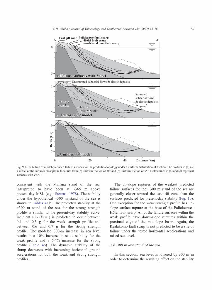
Fig. 9. Distribution of model-predicted failure surfaces for the pre-Hilina topology under a uniform distribution of friction. The profiles in (a) are
a subset of the surfaces most prone to failure from (b) uniform friction of 308 and (c) uniform friction of 558. Dotted lines in (b) and (c) representsurfaces with FsN1.
C.H. Okubo / Journal of Volcanology and Geothermal Research 138 (2004) 43–76 63
consistent with the Mahana stand of the sea,
interpreted to have been at ~365 m above
present-day MSL (e.g., Stearns, 1978). The stability
under the hypothetical +300 m stand of the sea is
shown in Tables 4a,b. The predicted stability at the
+300 m stand of the sea for the strong strength
profile is similar to the present-day stability curve.
Incipient slip (Fs=1) is predicted to occur between
0.4 and 0.5 g for the weak strength profile and
between 0.6 and 0.7 g for the strong strength
profile. The modeled 300-m increase in sea level
results in a 10% increase in static stability for the
weak profile and a 6.4% increase for the strong
profile (Table 4b). The dynamic stability of the
slump decreases with increasing horizontal ground
accelerations for both the weak and strong strength
profiles.
The up-slope ruptures of the weakest predicted
failure surfaces for the +300 m stand of the sea are
generally closer toward the east rift zone than the
surfaces predicted for present-day stability (Fig. 10).
One exception for the weak strength profile has up-
slope surface rupture at the base of the Poliokeawe–
Holei fault scarp. All of the failure surfaces within the
weak profile have down-slope ruptures within the
proximal edge of the mid-slope basin. Again, the
Kealakomo fault scarp is not predicted to be a site of
failure under the tested horizontal accelerations and
raised sea level.
3.4. 300 m low stand of the sea
In this section, sea level is lowered by 300 m in
order to determine the resulting effect on the stability
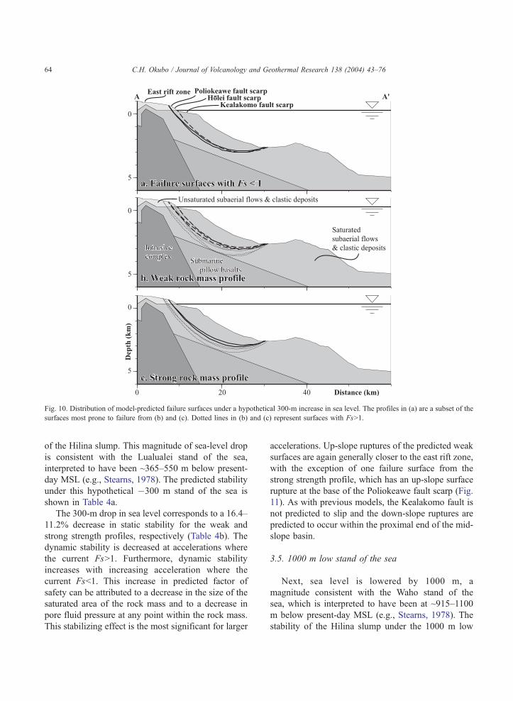
Fig. 10. Distribution of model-predicted failure surfaces under a hypothetical 300-m increase in sea level. The profiles in (a) are a subset of the
surfaces most prone to failure from (b) and (c). Dotted lines in (b) and (c) represent surfaces with FsN1.
C.H. Okubo / Journal of Volcanology and Geothermal Research 138 (2004) 43–7664
of the Hilina slump. This magnitude of sea-level drop
is consistent with the Lualualei stand of the sea,
interpreted to have been ~365–550 m below present-
day MSL (e.g., Stearns, 1978). The predicted stability
under this hypothetical �300 m stand of the sea is
shown in Table 4a.
The 300-m drop in sea level corresponds to a 16.4–
11.2% decrease in static stability for the weak and
strong strength profiles, respectively (Table 4b). The
dynamic stability is decreased at accelerations where
the current FsN1. Furthermore, dynamic stability
increases with increasing acceleration where the
current Fsb1. This increase in predicted factor of
safety can be attributed to a decrease in the size of the
saturated area of the rock mass and to a decrease in
pore fluid pressure at any point within the rock mass.
This stabilizing effect is the most significant for larger
accelerations. Up-slope ruptures of the predicted weak
surfaces are again generally closer to the east rift zone,
with the exception of one failure surface from the
strong strength profile, which has an up-slope surface
rupture at the base of the Poliokeawe fault scarp (Fig.
11). As with previous models, the Kealakomo fault is
not predicted to slip and the down-slope ruptures are
predicted to occur within the proximal end of the mid-
slope basin.
3.5. 1000 m low stand of the sea
Next, sea level is lowered by 1000 m, a
magnitude consistent with the Waho stand of the
sea, which is interpreted to have been at ~915–1100
m below present-day MSL (e.g., Stearns, 1978). The
stability of the Hilina slump under the 1000 m low

Fig. 11. Distribution of model-predicted failure surfaces under a hypothetical 300-m decrease in sea level. The profiles in (a) are a subset of the
surfaces most prone to failure from (b) and (c). Dotted lines in (b) and (c) represent surfaces with FsN1.
C.H. Okubo / Journal of Volcanology and Geothermal Research 138 (2004) 43–76 65
stand of the sea is similar to the present-day stability
(Table 4a). The transition from stable to predicted
slip occurs between 0.4 and 0.5 g for the weak
profile and occurs between 0.6 and 0.7 g for the
strong profile. Static stability decreases by 29.4–
22.3% for the weak and strong strength profiles,
respectively compared with the present-day stability
(Table 4b). Dynamic stability generally increases
with increasing acceleration, while decreasing at low
horizontal accelerations.
The geometries of some failure surfaces (with a
Fsb1) at the 1000 m low stand are significantly
different from previous predictions (Fig. 12). For the
strong profile, up-slope failure surface rupture is
predicted at either the Kealakomo fault scarp, or at a
scarp-like step offshore of the present-day coastline.
Further, the down-slope ruptures of these surfaces are
predicted to be near the distal end of the outer bench
slope, well beyond the mid-slope basin and mid-slope
bench. Ruptures within these areas are not predicted in
previous stability models that have smaller magnitudes
of sea-level change. Within the strong strength profile,
failure is predicted along a surface that ruptures up-
slope at Kealakomo and down-slope at the proximal
end of the mid-slope basin. A second failure surface is
predicted to rupture up-slope between the Poliokeawe
fault scarp and the east rift zone and down-slope within
the outer bench slope. Interestingly, failure surfaces are
not predicted to rupture through the base of the
Poliokeawe or Holei fault scarps.
The preceding analyses of various sea-level sce-
narios suggest that under the range of observed sea-
level variations in Hawai’i, the stability of the Hilina
slump is predicted to remain comparable to the
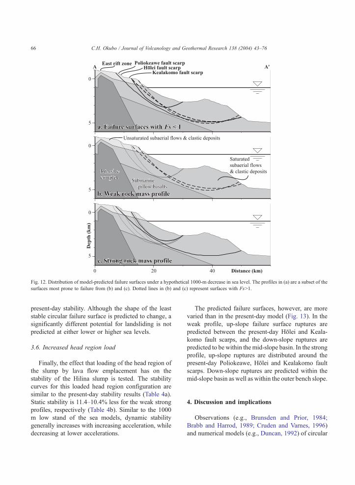
Fig. 12. Distribution of model-predicted failure surfaces under a hypothetical 1000-m decrease in sea level. The profiles in (a) are a subset of the
surfaces most prone to failure from (b) and (c). Dotted lines in (b) and (c) represent surfaces with FsN1.
C.H. Okubo / Journal of Volcanology and Geothermal Research 138 (2004) 43–7666
present-day stability. Although the shape of the least
stable circular failure surface is predicted to change, a
significantly different potential for landsliding is not
predicted at either lower or higher sea levels.
3.6. Increased head region load
Finally, the effect that loading of the head region of
the slump by lava flow emplacement has on the
stability of the Hilina slump is tested. The stability
curves for this loaded head region configuration are
similar to the present-day stability results (Table 4a).
Static stability is 11.4–10.4% less for the weak strong
profiles, respectively (Table 4b). Similar to the 1000
m low stand of the sea models, dynamic stability
generally increases with increasing acceleration, while
decreasing at lower accelerations.
The predicted failure surfaces, however, are more
varied than in the present-day model (Fig. 13). In the
weak profile, up-slope failure surface ruptures are
predicted between the present-day Holei and Keala-
komo fault scarps, and the down-slope ruptures are
predicted to be within the mid-slope basin. In the strong
profile, up-slope ruptures are distributed around the
present-day Poliokeawe, Holei and Kealakomo fault
scarps. Down-slope ruptures are predicted within the
mid-slope basin as well as within the outer bench slope.
4. Discussion and implications
Observations (e.g., Brunsden and Prior, 1984;
Brabb and Harrod, 1989; Cruden and Varnes, 1996)
and numerical models (e.g., Duncan, 1992) of circular

Fig. 13. Distribution of model-predicted failure surfaces under a simulated loading of the head region of the slump by lava flow emplacement.
The profiles in (a) are a subset of the surfaces most prone to failure from (b) and (c). Dotted lines in (b) and (c) represent surfaces with FsN1.
C.H. Okubo / Journal of Volcanology and Geothermal Research 138 (2004) 43–76 67
failures show that the up-slope rupture of circular
failure surfaces are characterized by normal faulting
and that the down-slope ruptures are characterized by
thrust faulting. The model-predicted locations of up-
slope ruptures under present-day conditions corre-
spond with the base of the Poliokeawe–Holei normal
fault scarp. This spatial correlation is consistent with
expected normal faulting within the head scarp region
of a circular failure. Therefore, the model failure
surfaces quantitatively show, from slope stability
analysis, that the Poliokeawe–Holei normal fault scarp
can be the head scarp for a plausible circular failure,
as has been previously hypothesized based on surface
morphology (e.g., Smith et al., 1999; Morgan et al.,
2003).
Slope stability predictions for the range of sea
levels and slope geometries tested here suggest that
several distinct failure surface geometries may be
unstable within the Hilina slump. After ruling out
failure geometries that do not intersect observed fault
scarps, such as the potential failure surfaces between
the east rift zone and Poliokeawe–Holei, there remain
several potential failure surfaces that intersect
observed or interpreted subaerial fault scarps. The
prediction of multiple failure surfaces under varying
slope, sea level, and dynamic loads suggests that there
may be multiple failure surfaces within the Hilina
slump that are activated or abandoned as sea level and
slope geometry changes. Essentially, the Hilina slump
may fail and deform along multiple internal failure
surfaces, rather than along a single surface.
Multiple failure surfaces can be readily accommo-
dated through slip along the multitude of preexisting
discontinuities within the rock mass of the slump.
C.H. Okubo / Journal of Volcanology and Geothermal Research 138 (2004) 43–7668
Post-peak values of RMR for a Hawaiian volcano are
not predicted to be significantly weaker than the
surrounding rock mass (Table 1). Thus, propagation of
an additional, favorably oriented slip surface may
require less driving stress than slip along a preexisting
(but non-optimally oriented) failure surface would.
This would lead to the growth of multiple failure
surfaces within the slide. Multiple slip surfaces of
different ages and levels of activity within a single
slide mass have been previously documented else-
where (e.g., Brunsden and Prior, 1984; Eisbacher and
Clague, 1984; Brabb and Harrod, 1989; Millet et al.,
1992).
The Kealakomo fault scarp, which is stable at all
tested accelerations under present-day conditions,
may be an example of a failure surface that was
abandoned as slope geometry and sea-level changes
rendered its corresponding slump block stable. Fault-
ing through the location of the Kealakomo fault scarp
is predicted in stability models using the pre-Hilina
topology and where the head region of the slump is
loaded by lava flow emplacement. The down-slope
rupture in this case is within the outer bench slope.
Thus, slip along the Kealakomo fault scarp and along
potential thrust faults within the outer bench slope
may have acted to stabilize older slump block
geometries. Once fault slip reduced these older
geometries to near present-day form, the Kealakomo
and any active submarine thrusts may have been
abandoned. This scenario is consistent with interpre-
tations by Morgan et al. (2003), who identify a
stabilized pre-Hilina slump to the east of the modeled
profile.
The Kealakomo fault scarp also coincides with two
potential failure surfaces in the 1000-m low stand
models. The up-slope rupture of one failure surface
that intersects Kealakomo has predicted down-slope
rupture at the proximal end of the mid-slope basin.
The down-slope rupture of the other surface is within
the outer bench slope, coincident with the location of
the down-slope rupture for the loaded head region
model. These results suggest that a decrease in MSL
on the order of 1000 m may also induce reactivation
of slip along the Kealakomo fault under the present-
day slope geometry.
Results of the 1000 m low stand, head loading, and
pre-Hilina models support the hypothesis that the
Kealakomo fault scarp has been abandoned due to its
relative stability under present-day conditions. Future
activity along Kealakomo may occur if sea level drops
sufficiently (by 300–1000 m), or if sufficient lava
flows are emplaced on the coastal plain seaward of the
Poliokeawe–Holei fault scarp.
The loaded head region and present-day stability
models suggest that slip along the Kealakomo fault
scarp may be driven by non-catastrophic, but pro-
gressive slope failure. These cycles are driven by head
region loading by lava flow emplacement, slip along a
circular failure surface, eventual stabilization of the
slump, and re-burial of the head region. Additionally,
slip initiation is predicted to be dependent upon
significant ground accelerations, which further con-
tributes to the cyclicity of the failure process. This
proposed scenario implies that burial of the head
region by younger lava flows may be an important
part of Hilina fault scarp growth. In this way, the
Poliokeawe and Holei faults may also eventually be
abandoned as the circular failures that they define
become stable.
4.1. Seismicity of the Hilina fault system
Based on numerical model predictions for the
present-day stability of the Hilina slump, the potential
for future slip along specific Hilina faults can be
assessed. The present-day stability models predict that
the Poliokeawe and Holei normal fault scarps are
susceptible to future slip due to horizontal ground
accelerations in excess of ~0.4–0.6 g. Conversely, the
Kealakomo normal fault scarp is predicted to be stable
against slip for ground accelerations up to 1.0 g (the
maximum tested acceleration). The Poliokeawe and
Holei fault scarps are predicted to continue to increase
in vertical displacement until attendant changes in
slope geometry stabilize the current failure surfaces.
Changes in sea level may also act to stabilize these
failure surfaces; however stability models predict that
changes in MSL exceeding 300 m are required to
do so.
The present-day potential for slip along thrust
faults at the toe of the slide can also be assessed. In all
tested cases, models of present-day conditions suggest
that thrust faulting is predicted to occur within the
proximal end of the mid-slope basin. Thrust faulting
through the outer bench slope is not predicted under
present-day conditions, implying that the observed
C.H. Okubo / Journal of Volcanology and Geothermal Research 138 (2004) 43–76 69
thrust faults in this region are either unrelated to the
failure surface of the Hilina slump (Morgan et al.,
2000; 2003; Hills et al., 2002) or are currently
inactive.
The predicted tendency for the Poliokeawe and
Holei faults to slip under horizontal ground accel-
erations from distal earthquakes is consistent with
previous observations of earthquake-induced land-
sliding in various geologic settings (e.g., Plafker et al.,
1971; Normark, 1974; Field et al., 1982; Keefer,
1984; Kenyon, 1987; Crespo et al., 1991). The role of
horizontal ground accelerations in triggering land-
slides has also been the subject of probabilistic
assessments of landslide hazard (e.g., Ziony et al.,
1985; Wilson and Keefer, 1985; Jibson and Keefer,
1993).
Earthquake-triggered landslides have been
observed in Hawai’i. In 1868, a Mfa 7.9 earthquake
in occurred in the Ka’u region along the southwest rift
zone of Kılauea volcano (Fig. 2; Hitchcock, 1912;
Wood, 1914; Stover and Coffman, 1993). First-person
accounts suggest that perceptible ground shaking
persisted for ~30 s, during which time a large
landslide occurred along the flank of neighboring
Mauna Loa volcano (Hitchcock, 1912; Wood, 1914).
The displaced rock mass of this slide was reported to
be as much as 3 km wide, 5 km long and 9 m thick
(Hitchcock, 1912; Wood, 1914). Smaller landslides
also occurred throughout the island. The epicenter of
the earthquake is interpreted to have been ~10 km
offshore (Fig. 2; Stover and Coffman, 1993), about 30
km south of the landslide.
Significantly, following the 1868 Ka’u earthquake,
fresh fault slip, of unreported magnitude, was
observed along the northern-most faults of the Hilina
fault system (Hitchcock, 1912), including the Polio-
keawe fault. Further, up to 2 m of coastal subsidence
was observed in the proximity of the model profile,
but the Kealakomo fault did not show fresh ruptures
(Hitchcock, 1912).
Based on reports of shaking intensity, an interpreted
Modified Mercalli Intensity of X (Wood, 1914) and
post-seismic damage assessment, Stover and Coffman
(1993) estimate ground accelerations of ~1 g at
Keaiwa, which is ~30 km northeast from the epicenter.
The Poliokeawe and Holei faults shown in the model
profile are another ~30 km northeast of Keaiwa. From
published firsthand reports, Wood (1914) suggests that
ground shaking with a Modified Mercalli Intensity of
X encompassed the entire Hilina fault system.
A Ms 7.2 earthquake at Kalapana in 1975 also
showed that the Poliokeawe and Holei faults are
susceptible to incremental slip due to ground accel-
erations, and that the Kealakomo is relatively stable.
The epicenter of this event was located about 30 km
east of the Hilina fault system and 15 km east of the
model profile (Fig. 2). Coseismic subsidence along
the Hilina faults was recorded by leveling and
trilateration (Lipman et al., 1985). Earthquake-related
faulting occurred on northern Hilina faults of Polio-
keawe and Holei, while faults closer to the coast (e.g.,
Kealakomo) did not rupture. Along the strand of the
Poliokeawe fault transected by the model profile,
1.5F0.5 m of down to the south normal fault
displacement was recorded after the earthquake, and
b1 m of vertical displacement was recorded along the
adjacent section of the Holei fault (Tilling et al.,
1976). Approximately 25 km of the northern-most
preexisting Hilina faults showed evidence of fresh slip
in the form of freshly broken rocks and soil and torn
vegetation (Tilling et al., 1976). Surface displace-
ments along the southwestern-most 5 km of this
rupture zone were related to fault propagation with as
much as 1 m vertical offset (Tilling et al., 1976). Slip
vectors for these offsets have shallow plunges (~208)consistent with slip along a circular Hilina failure
surface at a shallow depth (Cannon and Bqrgmann,
2001; Cannon et al., 2001).
Seismic loading from the 1975 Kalapana earth-
quake is proposed as the direct cause of the observed
slip on the Hilina faults (Lipman et al., 1985).
Although a few strong motion seismometers (SMA)
were in operation at the time, only three registered the
event. The closest SMA (three component) was
located 43 km away in Hilo, and registered a
maximum horizontal acceleration of 0.22 g (Rojahn
and Morrill, 1977).
Intense aftershock activity following the 1975
Kalapana earthquake was focused within an elongate
belt surrounding the northern-most faults of the Hilina
system (Tilling et al., 1976). This belt is distinctly
offset to the west of the 1975 Kalapana epicenter.
Following an earlier M 6.5 earthquake at Kalapana in
1954 (Fig. 2), through 1975, several M 4–5 earth-
quakes occurred along the south flank of Kılauea. In
each case, when the primary epicenter was to the east
C.H. Okubo / Journal of Volcanology and Geothermal Research 138 (2004) 43–7670
of the Hilina fault system, aftershock activity was
offset to the west and focused along the Hilina fault
system, and where the epicenter was located in the
central part of the Hilina, aftershocks were focused
within the eastern part of the Hilina (Tilling et al.,
1976). No earthquakes or aftershocks NM 4 occurred
along the coastal faults of the Hilina (e.g., Keala-
komo) between 1950 and 1975 (Tilling et al., 1976).
Isoseismal maps of Wyss and Koyanagi (1992)
provide additional predictions of the magnitude and
distribution of ground accelerations within the Hilina
fault system during the 1975 and 1868 earthquakes.
The 1975 Kalapana earthquake is estimated to have
resulted in MMI of VII to VIII throughout the Hilina,
with stronger shaking in the eastern half of the fault
system. The 1868 Ka’u earthquake is predicted to
have resulted in a MMI of IX–X within the Hilina
fault system, with the greatest intensity of shaking
near the coast. Relations between MMI values and g,
based on concurrent felt reports and instrumented
observations (e.g., Trifunac and Brady, 1975; Krinitz-
sky and Chang, 1988; Wyss and Koyanagi, 1992)
suggest that the shaking intensity for the 1975
Kalapana earthquake loosely corresponds to horizon-
tal ground accelerations of 0.1–0.6 g within the Hilina
fault system. These relations also suggest that the
1868 Ka’u earthquake resulted in horizontal ground
accelerations of 0.3–1.0 g within the Hilina. The mid
to upper ranges of these estimated ground acceler-
ations are within the critical 0.4–0.6 g range required
by the present-day stability models to initiate slip
along the northern-most Hilina faults of Poliokeawe
and Holei.
The seismicity of Kılauea’s south flank between
1950 and 1976 is consistent with stability model
predictions of distal earthquake-induced slip along the
faults of the Hilina system. Tilling et al. (1976) make
the observation that aftershocks within this time
period were focused along the northern-most faults
of the Hilina (e.g., the Poliokeawe and Holei), and
that no aftershocks were recorded around the faults
closer to the coast. Assuming that these aftershocks
are due to slip along faults of the Hilina system, this
observation can now be explained. The stability
models predict that the Poliokeawe and Holei fault
scarps are susceptible to earthquake-induced slip and
therefore are preferred sites for aftershock local-
ization. On the other hand, the more coastal Keala-
komo scarp is stable and not predicted to slip. Thus,
model-predicted stability of the coastal Hilina faults
can explain the observed gap in aftershocks around
faults nearest to the coast.
Based on the predicted failure plane geometries for
present-day conditions, seismicity related to slip along
the Hilina faults is predicted to be shallow, between 0
and ~3.5 km depth below present-day sea level. This
predicted depth range for Hilina-related seismicity
shows excellent correspondence with a shallow zone
of hypocenter localization below the Hilina for
earthquakes recorded between 1971 and 1989 that
are NM 1.5, as presented by Denlinger and Okubo
(1995). A relatively sparse gap in seismicity occurs
between ~3.5 and ~6 km depth, separating the
shallower Hilina seismic zone from a deeper zone
interpreted as evidence of slip along a detachment at
the base of the edifice (Got et al., 1994; Denlinger and
Okubo, 1995). No continuous spatial link in recorded
seismicity is apparent between the shallow and deep
seismic zones, as would be expected if these two
zones were structurally linked.
Assuming a circular failure geometry, the sense of
slip along faults of the present-day Hilina system is
predicted to vary predictably with distance, and depth,
from the base of the Poliokeawe–Holei fault scarp.
Normal fault displacements are predicted within ~15
km seaward of, and ~3.5 km depth below, the
Poliokeawe–Holei. Thrust displacements are pre-
dicted to occur between ~15 and ~20 km seaward of
Poliokeawe–Holei scarp and within ~2.5 to ~3.5 km
depth below sea level. Present-day Hilina-related
thrust faulting is therefore predicted to be confined
to the mid-slope basin. Faulting in the distal outer
bench slope is not predicted to be directly related to
present-day movement of the Hilina slump. Rather,
growth of the mid-slope bench may be a result of
accretion due to basal sliding of Kılauea’s south flank
(e.g., Morgan et al., 2000, 2003; Hills et al., 2002),
possibly in combination with past Hilina-driven
thrusting under different slope or sea-level conditions.
Interpretations of the character of displacements
along the basal edifice detachment have been based
on investigations of the Ms 7.2 1975 Kalapana
earthquake and an earlier Ms 6.1 earthquake near
Kalapana in 1989. Focal mechanism solutions indi-
cate thrust-related displacements for both events (Got
et al., 1994; Denlinger and Okubo, 1995). Further
C.H. Okubo / Journal of Volcanology and Geothermal Research 138 (2004) 43–76 71
evidence of thrust-related displacements for these two
events comes from dislocation models of the 1989
earthquake (Arnadottir et al., 1991, Delaney et al.,
1993) and tsunami generation models for the 1975
earthquake (Hatori, 1976; Ma et al., 1999).
Interpreted thrust-related displacements along a
basal edifice detachment are consistent with seaward
movement of Kılauea’s south flank due to dike
injection along its rift zones (Swanson et al., 1976;
Lipman et al., 1985). The present-day failure surface
geometries presented here, as well as the distribution
of seismicity presented by Denlinger and Okubo
(1995), do not support a structural link between the
Hilina faults and this detachment however; the slump
rides on top of the mobile flank instead. The
distribution of aftershocks and ground ruptures in
and around the faults of the Hilina system following
the 1975 Kalapana earthquake suggests a seismic
triggering relationship between the deeper basal
detachment and the shallower Hilina faults instead.
That is, ground accelerations due to slip along the
basal detachment may trigger slip along failure
surfaces of the Hilina slump. Thus, slip along the
Hilina slump may be triggered by dynamic (and
possibly static) stress change due to slip along the
subjacent basal detachment.
The slope stability analyses presented here predict
that the Hilina slump is stable under static conditions
and is susceptible to slip under horizontal ground
accelerations greater than 0.4 g–0.6 g. Consistent with
model predictions, historic observations demonstrate
that slip along the Poliokeawe and Holei faults can be
attributed to horizontal ground accelerations generated
by distal earthquakes of sufficient magnitude. Further,
the model-predicted stability of the Hilina slump can
account for the observed localization of aftershocks
near the Poliokeawe and Holei faults and for the
observed gap in aftershocks around the more seaward
faults (e.g., Kealakomo). The predicted depth range for
Hilina-related faulting can also account for observed
depth-dependent localizations of earthquakes.
4.2. Effects of mechanical stratigraphy
In all tested cases, predicted failure surfaces are
confined to the saturated and unsaturated subaerial
flows and clastic deposits units. No failure surfaces
with factors of safety less than one were predicted to
cut through the subjacent submarine pillow basalts,
intrusive complex, or oceanic crust units. The
subaerial flows and clastic deposits units have the
lowest frictional strength of all the modeled units due
to their relatively shallow depth and are therefore
most susceptible to faulting. It is not unexpected
therefore, that the weakest failure surfaces are con-
fined to the mechanically weakest unit.
Several previous works have suggested that the
faults of the Hilina system sole into a mechanically
weak detachment at the interface between the volcanic
edifice and oceanic crust (Lipman et al., 1985; Moore
et al., 1994, 1995). In order to test the effect of such a
detachment, a 100-m-thick mechanically weak layer is
added along the top of the oceanic crust unit, using the
present-day slope and sea level. The mechanically
weak unit is prescribed to be cohesionless, with an
internal friction angle of 308 and alternatively 108,consistent with saturated cohesionless sand or non-
plastic silt (e.g., Holtz and Kovacs, 1981). This
configuration is tested with both the strong and the
weak strength profiles using the Bishop and Janbu
methods.
The calculated factors of safety for both friction
angle models are within 1% of the present-day results
obtained with the non-detachment configuration (i.e.,
Fig. 5). The resulting failure surface geometries are
also consistent with the non-detachment case (i.e., the
present-day stability model, Fig. 6). Therefore, the
mechanically weak detachment is not favored as a
potential failure plane for the Hilina slump under
horizontal accelerations from 0 to 1.0 g.
5. Conclusions
The slope stability analysis presented here provides
a mechanics-based test for previous interpretations of
evidence for a circular failure style of deformation
within the Hilina slump. These analyses show that slip
along the Poliokeawe and Holei normal fault scarps
are plausibly the result of gravity and seismically
driven slump block displacements along a circular
failure surface under present-day slope and sea-level
conditions. Most importantly, the stability models
predict that the active circular failure surface for the
Hilina slump is structurally isolated from any basal
edifice detachment.
C.H. Okubo / Journal of Volcanology and Geothermal Research 138 (2004) 43–7672
Deformation of the Hilina slump block is
hypothesized here to be accommodated along multi-
ple internal failure surfaces. The geometry of
actively slipping failure surfaces varies in response
to changes in slope geometry, sea level, and ground
accelerations. Preexisting failure surfaces may
become stable and abandoned in favor of other
preexisting, or new, failure surfaces. Propagation of
new failure surfaces is expected to be facilitated by
slip along preexisting discontinuities within the rock
mass.
The Poliokeawe and Holei scarps are shown to
be favored sites of faulting for the present-day,
loaded head region, and F300 m sea-level change
models, for various subjacent failure surface geo-
metries. These scarps are susceptible to future slip
due to horizontal ground accelerations in excess of
0.4–0.6 g under these various model configurations.
These critical values of ground acceleration may be
reduced by transient variations in pore pressure, the
affects of which were not evaluated in this paper.
The Kealakomo normal fault is predicted to be the
site of faulting only within the separate scenarios of
a loaded head region, a sea level 1000 m below
present-day, and under a postulated pre-Hilina top-
ology.
Consistent with the present-day model predic-
tions, evidence of fresh slip along faults of the Hilina
system was observed following the 1868 Ka’u and
1974 Kalapana earthquakes. Further, the distribution
of aftershocks between 1950 and 1976 is consistent
with the predicted tendency for earthquake-induced
slip along the Poliokeawe and Holei fault scarps,
with no observed slip along the Kealakomo scarp.
Accordingly, the Poliokeawe and Holei scarps are
predicted to have the greatest potential for slip in the
near future. The predicted depth range for Hilina-
related seismicity can also account for observed
depth-dependent localizations of earthquakes. Seis-
micity related to slip along the Hilina fault scarps is
predicted to be within 3.5-km depth of present-day
sea level.
Stability models of the present-day conditions,
the pre-Hilina topology, and the loaded head region
configuration suggest that slip along the faults of
the Hilina system may be driven by cycles of head
region loading by lava flow emplacement, slip
along a circular failure surface, eventual stabiliza-
tion of the slump, and re-burial of the head region.
Therefore, present-day apparent offsets of the Hilina
faults may not correspond to true geologic displace-
ments because of cyclic fault scarp burial and
growth.
Based on the present-day failure surface geo-
metries presented here, as well as the distribution of
seismicity presented by Denlinger and Okubo (1995),
the faults of the Hilina system are interpreted as
structurally detached from a frictionally slipping
subjacent detachment along the base of the volcanic
edifice. Slope stability analyses provide no evidence
of fault linkage between these two sets of structures
under all tested slope and sea-level configurations.
Therefore, a weak basal detachment is not a prereq-
uisite for slope failure of the edifice. Observations of
coseismic deformation, and stability model predic-
tions, do suggest however that dynamic stress changes
due to slip along the basal detachment induce slip
along failure surfaces of the Hilina slump. If dike
injection drives seaward movement of Kılauea’s south
flank as previously suggested (e.g., Swanson et al.,
1976; Lipman et al., 1985), then triggered movement
of the Hilina slump may in this way be affected by
Kılauea’s magmatic processes. Additionally, ground
accelerations due to sufficiently energetic explosive
eruptions may also trigger slip.
Although the actual geometry of the active Hilina
failure surface is likely to be more complex than the
simple circular failure surfaces modeled here, these
analyses provide valuable, initial quantitative slope
stability assessments. The major conclusion of this
paper is that the predicted present-day failure
surfaces of the Hilina slump are shallow, located at
less than ~3 km depth. The Hilina faults are not
predicted to be structurally linked to a subjacent
detachment at the base of the edifice, and therefore
slip along this detachment is not structurally linked
to attendant slip along the Hilina faults. The Hilina
slump is thus envisioned to ride atop the south flank
of Kılauea as it moves seaward along a slipping
basal detachment, a process in line with previous
independent interpretations (Swanson et al., 1976;
Smith et al., 1999; Morgan et al., 2003). Under
present-day slope and sea-level configurations, hor-
izontal ground accelerations in excess of ~0.4–0.6 g
are predicted to cause movement along faults of the
Hilina slump.
C.H. Okubo / Journal of Volcanology and Geothermal Research 138 (2004) 43–76 73
Acknowledgements
Thoughtful and thorough reviews by Juli Morgan
and an anonymous reviewer significantly improved the
flow and logic of this paper. Thanks are due to John
Smith and Terri Duennebier for providing the digital
terrain model for the island of Hawai’i. Thanks also to
Gregg Stefanelli for computing support, to GregMoore
and P. Eeps for insightful discussions, and to Darcy Hu,
Jade Nakamura and Laura Schuster for expediting
research permits in Hawai’i Volcanoes National Park.
Robert Watters provided laboratory testing equipment,
as well as an insightful critique of this paper. Addi-
tionally, Lionel Wilson provided a helpful editorial
review. Finally, thanks to Richard Schultz for introduc-
ing me to the mechanics of rock masses.
References
Ando, M., 1979. The Hawaii earthquake of November 29, 1975;
low dip angle faulting due to forceful injection of magma. J.
Geophys. Res. 84, 7616–7626.
Arnadottir, T., Segall, P., Delaney, P.T., 1991. A fault model for the
1989 Kilauea south flank earthquake from leveling and seismic
data. Geophys. Res. Lett. 18, 2217–2220.
Barton, N.R., 1976. The shear strength of rock and rock joints. Int.
J. Rock Mech. Min. Sci. 13, 255–279.
Bell, F.G., 1992. Engineering in Rock Masses. Butterworth-
Heinemann, Boston, MA, 580 pp.
Bieniawski, Z.T., 1976. Rock mass classification in rock engineer-
ing. Exploration for Rock Engineering. Proc. Symp., Cape
Town. Balkema, Cape Town, pp. 97–106.
Bieniawski, Z.T., 1978. Determining rock mass deformability:
experience from case histories. Int. J. Rock Mech. Min. Sci.
15, 237–247.
Bieniawski, Z.T., 1989. Engineering Rock Mass Classification.
Wiley, New York, 251 pp.
Bishop, A.W., 1955. The use of the slip circle in the stability
analysis of slopes. Geotechnique 5, 7–17.
Brabb, E.E., Harrod, B.L., 1989. Landslides: Extent and Economic
Significance. Balkema, Rotterdam, 385 pp.
Brace, W.F., Martin, R.J., 1968. A test of the law of effective stress
for crystalline rocks of low porosity. Int. J. Rock Mech. Min.
Sci. 5, 415–426.
Brigham, W.T., 1909. The volcanoes of Kilauea and Mauna Loa
on the Island of Hawaii. Bernice P. Bishop Mus. Mem. 2 (4)
222 pp.
Brunsden, D., Prior, D.B., 1984. Slope Instability. Wiley, New York,
620 pp.
Bye, A.R., Bell, F.G., 2001. Stability assessment and slope design at
Sandsloot open pit, South Africa. Int. J. Rock Mech. Min. Sci.
38, 449–466.
Cannon, E.C., Bqrgmann, R., 2001. Prehistoric fault offsets of the
Hilina fault system, south flank of Kilauea volcano, Hawaii.
J. Geophys. Res. 106, 4207–4219.
Cannon, E.C., Bqrgmann, R., Owen, S.E., 2001. Shallow normal
faulting and block rotation associated with the 1975 Kalapana
earthquake, Kilauea volcano, Hawaii. Bull. Seismol. Soc. Am.
91, 1563–1573.
Carracedo, J.C., 1999. Growth, structure, instability and collapse of
Canarian volcanoes and comparisons with Hawaiian volcanoes.
J. Volcanol. Geotherm. Res. 94, 1–19.
Carter, R.M., Carter, L., Johnson, D.P., 1986. Submergent shore-
lines in the SW Pacific; evidence for an episodic post-glacial
transgression. Sedimentology 33, 629–649.
Casadevall, T.J., Dzurisin, D., 1987. Stratigraphy and petrology of
the Uwekahuna Bluff section, Kılauea Caldera. In: Decker,
R.W., Wright, T.L., Stauffer, P.H. (Eds.), Volcanism in Hawai’i.
U.S. Geol. Surv., Prof. Pap. 1350, 351–375.
Cavounidis, S., 1987. On the ratio of factors of safety in slope
stability analyses. Geotechnique 37, 207–210.
Cervelli, P., Segall, P., Johnson, K., Lisowski, M., Miklius, A.,
2002. Sudden aseismic fault slip on the south flank of Kilauea
volcano. Nature 415, 1014–1018.
Cheng, C.H., Johnson, D.H., 1981. Dynamic and static moduli.
Geophys. Res. Lett. 8, 39–42.
Coulbourn, W.T., Campbell, J.F., Moberly, R., 1974. Hawaiian
submarine terraces, canyons, and Quaternary history evaluated
by seismic reflection profiling. Mar. Geol. 17, 215–234.
Crandell, D.R., 1989. Gigantic debris avalanche of Pleistocene age
from ancestral Mount Shasta volcano, California, and Debris-
avalanche hazard zonation. U.S. Geol. Surv. Bull. 1861, 32 pp.
Crespo, E., O’Rourke, T.D., Hyman, K.J., 1991. Effects on lifelines.
In: Schuster, R.L. (Ed.), The March 5, 1987 Ecuador Earth-
quakes. Committee on Natural Disasters, National Research
Council, Washington, DC, pp. 83–99.
Cruden, D.M., Varnes, D.J., 1996. Landslide types and processes.
Transportation Research Board Special Report 247, 36–75.
Decker, R.W., Christiansen, R.L., 1984. Explosive Erup-
tions of Kilauea volcano, Hawaii. In: National Research
Council (Ed.), Explosive Volcanism. Natl. Acad., Washington,
DC, pp. 122–132.
Deere, D.U., 1964. Technical description of rock cores for
engineering purposes. Rock Mech. Eng. Geol. 1, 17–22.
Delaney, P.T., Miklius, A., Arnadottir, T., Okamura, A.T., Sako,
M.K., 1993. Motion of Kılauea Volcano during sustained
eruption from the Pu’u ’O’o and Kupaianaha vents, 1983–
1991. J. Geophys. Res. 98, 17801–17820.
Denlinger, R.P., Okubo, P., 1995. Structure of the mobile south
flank of Kılauea volcano, Hawai’i. J. Geophys. Res. 100,
24499–24507.
de Voogd, B., Palome, S.P., Hirn, A., Charvis, P., Gallart, J.,
Rousset, D., Danobeitia, J., Perroud, H., 1999. Vertical move-
ments and material transport during hotspot activity: seismic
reflection profiling offshore La Reunion. J. Geophys. Res. 104,
2855–2874.
Duffield, W.A., Stieltjes, L., Varet, J., 1982. Huge landslide blocks
in the growth of Piton de la Fournaise, La Reunion, and Kılauea
Volcano, Hawai’i. J. Volcanol. Geotherm. Res. 12, 147–160.

C.H. Okubo / Journal of Volcanology and Geothermal Research 138 (2004) 43–7674
Duncan, J.M., 1992. State-of-the-art: static stability and defor-
mation analysis. Proc. ASCE Specialty Conference on Stability
and Performance of Slopes and Embankments II, Berkeley,
California. Am. Soc. Civil Eng., Geotech. Spec. Pub., vol. 31,
pp. 222–266.
Duncan, J.M., 1996. Soil slope stability analysis. Transp. Res.
Board Spec. Rep. 247, 337–371.
Duncan, J.M., Wright, S.G., 1980. The accuracy of equilibrium
methods of slope stability analysis. Eng. Geol. 16, 5–17.
Eaton, M., 1987. Stratigraphy of Kılauea volcano. In: Decker, R.W.,
Wright, T.L., Stauffer, P.H. (Eds.), Volcanism in Hawai’i. U.S.
Geol. Surv. Prof. Pap. 1350, 243–260.
Eisbacher, G.H., Clague, J.J., 1984. Destructive mass movements
in high mountains: hazard and management. Geol. Surv. Can.,
16–84.
Eisenhauer, A., Wasserburg, G.J., Chen, J.H., Bonani, G., Collins,
L.B., Zhu, Z.R., Wyrwoll, K.H., 1993. Holocene sea-level
determination relative to the Australian continent; U/Th (TIMS)
and (super 14) C (AMS) dating of coral cores from the Abrolhos
Islands. Earth Planet. Sci. Let. 114, 529–547.
Ellis, W., 1827. Narrative of a Tour of Hawaii, or Owhyhee, with
Remarks on the History, Traditions, Manners, Customs, and
Language of the Inhabitants of the Sandwich Islands. Honolulu
Advertiser Pub. Co., Hawaii, 342 pp.
Elsworth, D., Day, S.J., 1999. Flank collapse triggered by intrusion;
the Canarian and Cape Verde archipelagoes. J. Volcanol.
Geotherm. Res. 94, 323–340.
Elsworth, D., Voight, B., 1995. Dike intrusion as a trigger for large
earthquakes and the failure of volcano flanks. J. Geophys. Res.
100, 6005–6024.
Field, M.E., Gardner, J.V., Jennings, A.E., Edwards, B.D., 1982.
Earthquake-induced sediment failures on a 0.25 degrees slope,
Klamath River delta, California. Geology 10, 542–546.
Forslund, T., Gudmundsson, A., 1991. Crustal spreading due to
dikes and faults in southwest Iceland. J. Struct. Geol. 13,
443–457.
Francis, P., Oppenheimer, C., Stevenson, D., 1993. Endogenous
growth of persistently active volcanoes. Nature 366, 554–557.
Garcia, M.O., 1996. Petrography and olivine and glass chemistry of
lavas from the Hawaii Scientific Drilling Project. J. Geophys.
Res. 101, 11701–11713.
Gibb, J.G., 1986. New Zealand regional Holocene eustatic sea-level
curve and its application to determination of vertical tectonic
movements. In: Reilly, W.I., Harford, B.E. (Eds.), Recent
Crustal Movements of the Pacific Region. Bull. Royal Soc.
New Zealand 24, 377–395.
Goodman, R.E., Shi, G.H., 1985. Block Theory and its Application
to Rock Engineering. Prentice-Hall, New Jersey, 338 pp.
Got, J.L., Frechert, J., Klein, F.W., 1994. Deep fault plane geometry
inferred from multiple relative relocation beneath the south flank
of Kilauea. J. Geophys. Res. 99, 15375–15386.
Gudmundsson, A., 1988. Effect of tensile stress concentration
around magma chambers on intrusion and extrusion frequencies.
J. Volcanol. Geotherm. Res. 35, 179–194.
Hatori, T., 1976. Wave source of the Hawai’i tsunami in 1975
and the tsunami behavior in Japan. J. Seismol. Soc. Jpn. 29,
355–364.
Hills, D.J., Morgan, J.K., Moore, G.F., Leslie, S.C., 2002. Structural
variability along the submarine south flank of Kılauea volcano,
Hawai’i, from a multichannel seismic reflection survey. AGU
Monogr. 128, 105–123.
Hitchcock, C.H., 1912. The Hawaiian earthquakes of 1868. Bull.
Seismol. Soc. Am. 2, 181–192.
Hoek, E., 1983. Strength of jointed rock masses. Geotechnique 33,
187–223.
Hoek, E., 1994. Strength of rock and rock masses. Int. Soc. Rock
Mech. New J. 2, 4–16.
Hoek, E., Bray, J.W., 1981. Rock Slope Engineering. Institution of
Mining and Metallurgy, London, 358 pp.
Hoek, E., Brown, E.T., 1980. Empirical strength criterion for
rock masses. J. Geotech. Eng. Div. Am. Soc. Civil Eng. 106,
1013–1335.
Hoek, E., Brown, E.T., 1988. The Hoek–Brown failure criterion—a
1988 update. Rock engineering for underground excavations.
Proc., 15th Canadian Rock Mech. Symp. Dept. Civil Engineer-
ing. University of Toronto, Toronto, pp. 31–38.
Hoek, E., Brown, E.T., 1997. Practical estimates of rock mass
strength. Int. J. Rock Mech. Min. Sci. 34, 1165–1186.
Hoek, E., Kaiser, P.K., Bawden,W.F., 1995. Support of Underground
Excavations in Hard Rock. Balkema, Rotterdam, 215 pp.
Holcomb, R.T., 1987. Eruptive history and long-term behavior of
Kılauea Volcano. In: Decker, R.W., Wright, T.L., Stauffer, P.H.
(Eds.), Volcanism in Hawai’i. U.S. Geol. Surv., Prof. Pap. 1350,
261–350.
Holtz, R.D., Kovacs, W.D., 1981. An Introduction to Geotechnical
Engineering. Prentice-Hall, New Jersey, 731 pp.
Hungr, O., 1987. An extension of Bishop’s simplified method of
slope stability analysis to three dimensions. Geotechnique 37,
113–117.
Hungr, O., Salgado, F.M., Byrne, P.M., 1989. Evaluation of a three-
dimensional method of slope stability analysis. Can. Geotech. J.
26, 679–686.
International Society for Rock Mechanics, 1975. Report of the
Commission on Terminology. International Society for Rock
Mechanics, Lisbon.
Iverson, R.M., 1995. Can magma injection and groundwater forces
cause massive landslides on Hawaiian volcanoes? J. Volcanol.
Geotherm. Res. 66, 295–308.
Jackson, D.B., Kauahikaua, J., 1987. Regional self potential
anomalies at Kılauea volcano. In: Decker, R.W., Wright, T.L.,
Stauffer, P.H. (Eds.), Volcanism in Hawai’i. U.S. Geol. Surv.,
Prof. Pap. 1350, 947–960.
Jaeger, J.C., Cook, G.W., 1979. Fundamentals of Rock Mechanics.
Chapman & Hall, London, 585 pp.
Janbu, N., 1954. Application of composite slip surfaces for stability
analysis. Proc. European Conf. on Stability of Earth Slopes,
Stockholm, pp. 43–49.
Jibson, R.W., Keefer, D.K., 1993. Analysis of the seismic origin of
landslides; examples from the New Madrid seismic zone. Geol.
Soc. Am. Bull. 105, 521–536.
Keefer, D.K., 1984. Landslides caused by earthquakes. Geol. Soc.
Am. Bull. 95, 406–421.
Kenyon, N.H., 1987. Mass wasting features on the continental slope
of Northwest Europe. Mar. Geol. 74, 57–77.
C.H. Okubo / Journal of Volcanology and Geothermal Research 138 (2004) 43–76 75
Klein, F.W., Frankel, A.D., Mueller, C.S., Wesson, R.L., Okubo,
P.G., 2001. Seismic Hazard in Hawai’i: high rate of large
earthquakes and probabilistic ground motion maps. Bull.
Seismol. Soc. Am. 91, 479–498.
Krinitzsky, E.L., Chang, F.K., 1988. Intensity related earthquake
ground motions. Bull. Assoc. Eng. Geol. 25, 425–435.
Ku, T.L., Kimmel, M.A., Easton, W.H., O’Neil, T.J., 1974. Eustatic
sea level 120,000 years ago on O’ahu, Hawai’i. Science 183,
959–962.
Lade, P.V., de Boer, R., 1997. The concept of effective stress for
soil, concrete and rock. Geotechnique 47, 61–78.
Lama, R.D., Vutukuri, V.S., 1978. Handbook on Mechanical
Properties of Rocks vol. II. Trans Tech Publications, Switzerland,
481 pp.
Law, K.T., Holtz, R.D., 1978. A note on Skempton’s A parameter
with rotation of principal stresses. Geotechnique 28, 57–64.
Leslie, S.C., Moore, G.F., Morgan, J.K., Hills, D.J., 2002. Seismic
stratigraphy of the Frontal Hawaiian Moat; implications for
sedimentary processes at the leading edge of an oceanic hotspot
trace. Mar. Geol. 184, 143–162.
Lipman, P.W., Mullineaux, D.R., 1981. The 1980 Eruption of
Mount St. Helens, Washington. U.S. Geol. Surv. Pap. 1250,
844 pp.
Lipman, P.W., Lockwood, J.P., Okamura, R.T., Swanson, D.A.,
Yamashita, K.M., 1985. Ground deformation associated with the
1975 magnitude-7.2 earthquake and resulting changes in activity
of Kılauea Volcano, Hawai’i. U.S. Geol. Surv., Prof. Pap. 1276,
45 pp.
Lopes, R., Guest, J.E., Hiller, K., Neukum, G., 1982. Further
evidence for a mass movement origin of the Olympus Mons
Aureole. J. Geophys. Res. 87, 9917–9928.
Lorig, L.J., Hart, R.D., Cundall, P.A., 1991. Slope stability analysis
of jointed rock using the distinct element method. Trans-
portation Research Board Research Record 1330, 1–9.
Kuo-Fong, Ma, Kanamori, H., Satake, K., 1999. Mechanism of the
1975 Kalapana, Hawaii, earthquake inferred from tsunami data.
J. Geophys. Res. 104, 13153–13168.
Mastin, L.G., 1997. Evidence for water influx from a
caldera lake during the explosive hydromagmatic eruption
of 1790. Kilauea volcano, Hawaii. J. Geophys. Res. 102,
20093–20109.
McPhie, J., Walker, G.P.L., Christiansen, R.L., 1990. Phreatomag-
matic and phreatic fall and surge deposits from explosions at
Kilauea Volcano, Hawaii, 1790 A.D.; Keanakakoi Ash Member.
Bull. Volcanol. 52, 334–354.
Millet, R.A., Lawton, G.M., Repetto, P.C., Garga, V.K., 1992.
Stabilization of Tablachaca Dam. In: Seed, R.B., Boulanger,
R.W. (Eds.), Stability and Performance of Slopes and Embank-
ments: Proceedings of a Specialty Conference. American
Society of Civil Engineers Geotechnical Special Publication,
vol. 31, pp. 1365–1381.
Moore, J.G., Clague, D.A., Holcomb, R.T., Lipman, P.W.,
Normark, W.R., Torresan, M.E., 1989. Prodigious submarine
landslides on the Hawaiian Ridge. J. Geophys. Res. 94,
17465–17484.
Moore, J.G., Normark, W.M., Holcomb, R.T., 1994. Giant Hawaiian
landslides. Annu. Rev. Earth Planet. Sci. 22, 119–144.
Moore, J.G., Bryan, W.B., Beeson, M.H., Normark, W.R., 1995.
Giant blocks in the South Kona landslide, Hawai’i. Geology 23,
125–128.
Morgan, J.K., Moore, G.F., Hills, D.J., Leslie, S., 2000. Over-
thrusting and sediment accretion along Kılauea’s mobile south
flank, Hawai’i: evidence for volcanic spreading from marine
seismic reflection data. Geology 28, 667–670.
Morgan, J.K., Moore, G.F., Clague, D.A., 2003. Slope failure and
volcanic spreading along the submarine south flank of Kilauea
volcano, Hawaii. J. Geophys. Res. 108, 2415, (doi:10.1029/
2003JB002411).
Morgenstern, N.R., Price, V.E., 1965. The analysis of the stability of
general slip surfaces. Geotechnique 15, 79–93.
Normark, W.R., 1974. Ranger submarine slide, Northern Sebastian
Vizcaino Bay, Baja California, Mexico. Geol. Soc. Am. Bull.
85, 781–784.
Norrish, N.I., Wyllie, D.C., 1996. Rock slope stability
analysis. Transportation Research Board Special Report 247,
391–428.
Okubo, C.H., Martel, S.J., 1998. Pit crater formation on Kılauea
Volcano, Hawai’i. J. Volcanol. Geotherm. Res. 86, 1–18.
Owen, S., Segall, P., Freymueller, J., Miklius, A., Denlinger, R.,
Arnadottir, T., Sako, M., Bqrgmann, R., 1995. Rapid deforma-
tion of the south flank of Kilauea volcano, Hawaii. Science 267,
1328–1331.
Owen, S., Segall, P., Lisowski, M., Miklius, A., Denlinger, R.,
Sako, M., 2000. Rapid deformation of Kilauea volcano: Global
Positioning System measurements between 1990 and 1996.
J. Geophys. Res. 105, 18983–18998.
Plafker, G., Ericksen, G.E., Concha, J.F., 1971. Geological aspects
of the May 31, 1970, Peru earthquake. Bull. Seismol. Soc. Am.
61, 543–578.
Priest, S.D., 1993. Discontinuity Analysis for Rock Engineering.
Chapman & Hall, London, 473 pp.
Priest, S.D., Hudson, J.A., 1976. Discontinuity spacings in rock. Int.
J. Rock Mech. Min. Sci. and Geomech. Abstr. 13, 135–148.
Riley, C.M., Diehl, J.F., Kirschvink, J.L., Ripperdan, R.L., 1999.
Paleomagnetic constraints on fault motion in the Hilina Fault
System, south flank of Kilauea Volcano, Hawaii. J. Volcanol.
Geotherm. Res. 94, 233–249.
Rojahn, C., Morrill, B.J., 1977. The island of Hawai’i earthquakes
of November 29, 1975: strong-motion data and damage
reconnaissance report. Bull. Seismol. Soc. Am. 67, 493–515.
Sarma, S.K., 1973. Stability analysis of embankments and slopes.
Geotechnique 23, 423–433.
Scholl, M.A., Ingebritsen, S.E., Janik, C.J., Kauahikaua, J.P., 1996.
Use of precipitation and groundwater isotopes to interpret
regional hydrology on a tropical volcanic island: Kilauea
volcano area, Hawaii. Water Resour. Res. 32, 3525–3537.
Schultz, R.A., 1995. Limits on strength and deformation proper-
ties of jointed basaltic rock masses. Rock Mech. Rock Eng.
28, 1–15.
Schultz, R.A., 1996. Relative scale and the strength and deform-
ability of rock masses. J. Struct. Geol. 18, 1139–1149.
Sharma, S.K., 1994. XSTABL, an Integrated Slope Stability
Analysis Program for Personal Computers: Reference Manual
Version 5. Interactive Software Designs, Moscow, ID. 214 pp.
C.H. Okubo / Journal of Volcanology and Geothermal Research 138 (2004) 43–7676
Skempton, A.W., 1954. The pore-pressure coefficients A and B.
Geotechnique 4, 143–147.
Smith, J.R, Malahoff, A., Shor, A.N., 1999. Submarine geology of
the Hilina slump and the morpho-structural evolution of Kılauea
Volcano, Hawai’i. J. Volcanol. Geotherm. Res. 94, 59–88.
Spencer, E., 1967. A method of analysis of the stability of
embankments assuming parallel inter-slice forces. Geotechnique
17, 11–26.
Sprigg, R.C., 1979. Stranded and submerged sea–beach systems of
Southeast South Australia and the aeolian desert cycle. Sedi-
ment. Geol. 22, 53–96.
Stearns, H.T., 1978. Quaternary shorelines in the Hawaiian Islands.
Bernice P Bishop Mus. Bull. 237, 57 pp.
Stearns, H.T., Easton, W.H., 1977. Radiocarbon profile of Hanauma
Reef, O’ahu, Hawai’i: discussion. Geol. Soc. Am. Bull. 88,
1535–1536.
Stearns, H.T., Macdonald, G.A., 1946. Geology and groundwater
resources of the Island of Hawai’i. Hawai’i Div. Hydrogr., Bull.
9. 194 pp.
Stover, C.W., Coffman, J.L., 1993. Seismicity of the United
States, 1568–1989 (revised). U. S. Geol. Surv. Prof. Pap. 1527,
201–213.
Swanson, D.A., Duffield, W.A., Fiske, R.S., 1976. Displacement of
the south flank of Kılauea volcano: the result of forceful
intrusion of magma into the rift zones. U. S. Geol. Surv. Prof.
Pap. 963, 39 pp.
Tilling, R.I., Koyanagi, R.Y., Lipman, P.W., Lockwood, J.P., Moore,
J.G., Swanson, D.A., 1976. Earthquake and related catastrophic
events, Island of Hawaii, November 29, 1975; a preliminary
report. U.S. Geol. Surv. Circ. 740, 32 pp.
Trifunac, M.D., Brady, A.G., 1975. On correlation of seismoscope
response with earthquake magnitude and modified Mercalli
intensity. Bull. Seismol. Soc. Am. 65, 307–321.
U.S. Department of Energy, 1988. Consultation draft, site character-
ization plan, reference repository location, Hanford site,
Washington. DOE-RW-0164.
Vallance, J.W., Scott, K.M., 1997. The Osceola mudflow from
Mount Rainier—sedimentology and hazard implications of a
huge clay-rich flow. Geol. Soc. Am. Bull. 109, 143–163.
Varnes, D.J., 1978. Slope movement types and processes. Transp.
Res. Board Spec. Rep. 176, 11–33.
Watters, R.J., Delahaut, W.D., 1995. Effect of argillic alteration of
rock mass stability. In: Haneberg, W.C., Anderson, S.A. (Eds.),
Reviews in Engineering Geology, vol. 10, pp. 139–150.
Watters, R.J., Zimbelman, D.R., Bowman, S.D., Crowley, J.K.,
2000. Rock mass strength assessment and significance to edifice
stability, Mount Rainier and Mount Hood, Cascade Range
volcanoes. Pure Appl. Geophys. 157, 957–976.
Wilson, R.C., Keefer, D.K., 1985. Predicting aerial limits
of earthquake-induced landsliding. In: Ziony, J.I. (Ed.), Eval-
uating Earthquake Hazards in the Los Angeles Region; An
Earth-Science Perspective. U. S. Geol. Surv. Prof. Pap. 1360,
317–345.
Wolfe, E.W., Morris, J. Geologic map of the Island of Hawaii, U.S.
Geol. Surv., Misc. Inv. Ser. Map I-2524-A (1996).
Wood, H.O., 1914. On the earthquakes of 1868 in Hawai’i. Bull.
Seismol. Soc. Am. 4, 169–203.
Wyss, M., Koyanagi, R.Y., 1992. Isoseismal maps, macro-
seismic epicenters, and estimated magnitudes of historical
earthquakes in the Hawaiian Islands. U.S. Geol. Surv. Bull.
2006, 93 pp.
Ziony, J.I., Evernden, J.F., Fumal, T.E., Harp, E.L., Hartzell, S.H.,
Joyner, W.B., Keefer, D.K., Spudich, P., Tinsley, J.C., Yerkes,
R.F., Youd, T.L., 1985. Predicted geologic and seismologic
effects of a postulated magnitude 6.5 earthquake along the
northern part of the Newport–Inglewood Zone. In: Ziony, J.I.
(Ed.), Evaluating Earthquake Hazards in the Los Angeles
Region; An Earth-Science Perspective. U. S. Geol. Surv. Prof.
Pap. 1360, 415–442.
Zucca, J.J., Hill, D.P., Kovach, R.L., 1982. Crustal structure of
Mauna Loa volcano, Hawai’i, from seismic refraction and
gravity data. Bull. Seismol. Soc. Am. 72, 1535–1550.