rode’s south african property trends

www.rode.co.zaPROPERTY CONSULTANTS, VALUERS& TOWN PLANNERS

&Associates

Rode’s South African Property Trends2019-2024

December 2019

Rode’s SA Property Trends Dec 2019 © i

Vol. 30 no.2 (December 2019)

CEO:Erwin G. Rode

Written and researched by: Kobus LamprechtEditor

CEOErwin G. Rode

EditorKobus Lamprecht

Technical Assistance Samantha Harkers-Kies

SubscriptionsJuwayra Januarie021 946 2480Annual subscription:2 issues: R20.550 (excl. VAT)

Published by Rode & Associates (Pty) Ltd. Reg. No: 2009/005600/07PO Box 1566, Bellville 7535 Tel. 021 946 2480 Fax 021 946 1238E-mail: [email protected]

Cover design Konrad Rode

082 446 6526

www.rodegraphics.com

Published twice a year

Only in electronic format

All rights reserved. No part of this publication

may be reproduced, stored in a retrieval

system, or transmitted in any form or by any

means, electronic, mechanical, photocopying,

recording or otherwise, without the

prior permission of the publisher.

While every precaution is taken to ensure the

accuracy of information, Rode & Associates

(Pty) Ltd. shall not be liable to any person for

inaccurate information or opinions contained

in this publication.

2019 - 2024A medium-term forecast and interpretation

of the crucial property variables

Rode’s SA Property Trends Dec 2019 © ii

Copyright

Copyright vests in Rode & Associates (Pty) Ltd. Our confidential reports are intended for your organisation's internal use. This implies that the forecasts may also be made available to your branch offices and for that purpose you may make as many copies of this report as you need. These forecasts may, however, not be divulged to outside parties, quoted in public, be provided to the media or be published in any form whatsoever.

Disclaimer

Great care has been taken with the compilation of this report. However, Rode

& Associates (Pty) Ltd. cannot be held responsible for any loss which might

result from accidentally inaccurate data and interpretations. Furthermore,

readers should note that all forecasts are subject to a margin of error. This

especially applies to medium-term forecasts.

iii Rode staff

Rode staff

Erwin RodeBA, MBA (Stell): CEO

Kobus LamprechtBCom ((NWU), BComHons and MCom (NWU)

Berchtwald RodeBA (Stell), MTRP (UOFS)

Juliana DommisseBEconHons (Stell)

Monique VernooyBTech(QS) (Cape Tech), NDREES (UNISA)

Binty Britz

BA (Stell), MLPM (UOFS)

Marlene TighyBSc (Wits) Hons (OR) (RAU), MBL (UNISA), Pr Sci Nat

Shimonay Jonas

Samantha Harkers

ND: HRM (CPUT)

Elizma Hawksley

Juwayra Januarie

Abigail Van Wyk

Lynette Smit

Rode’s SA Property Trends Dec 2019 ©

Stephan van der WaltMA (Stell)

iv

The difficulty lies not so much in developing new ideas as in escaping from old ones.

— John Maynard Keynes

Rode’s SA Property Trends Dec 2019 ©

Rode’s SA Property Trends Dec 2019 © v Table of contents

Table of contents

Executive Summary 1

Chapter 1 Rode’s econometric model 3

Chapter 2 Summary of the forecasts 4

Chapter 3: The property cycle Where are we in the long property cycle? 11

Chapter 4: The office market Office market woes will continue 16

Chapter 5: The industrial market Industrial market cools 22

Chapter 6: Retail property Retail sales growth slows to 10-year low 28

Chapter 7: The residential market House prices still battling to beat inflation 34

Chapter 8: Capitalization rates Capitalization rates will worsen 38

Chapter 9: Building activity and building costsBleak building activity outlook 42

Chapter 10: Total returns on directly-held property Total returns will head south 46

Chapter 11: Listed property Expect distributions to come under more pressure 50

Rode’s SA Property Trends Dec 2019 © vi List of tables

List of tables

5

6

7

8

9

10

12

19

20

20

21

25

26

26

26

30

31

32

32

37

37

39

40

43

43

44

45

Table 2.1: Baseline scenario: Results of Rode’s macroeconomic forecasts

s survey

Table 2.2: IMF scenario: Rode’s in-house forecast

Table 2.3: Forecast summary of the critical variables: Baseline scenario

Table 2.4: Forecast of real growth under Baseline scenario

Table 2.5: Baseline scenario: Average 6-year percentage change

Table 2.6: Forecast summary of the critical variables: IMF scenario

Table 3.1: Real GDP forecasts

Table 4.1: Baseline scenario: Forecast of grades A+, A & B office vacancies

Table 4.2: Baseline scenario: Forecast of nominal prime office rentals

Table 4.3: Baseline scenario: Forecast of real prime office rentals

Table 4.4: IMF scenario: Forecast of nominal prime office rentals

Table 5.1: Baseline scenario: Forecast of industrial vacancy factors

Table 5.2: Baseline scenario: Forecast of nominal prime industrial rentals

Table 5.3: Baseline scenario: Forecast of real prime industrial rentals

Table 5.4: IMF scenario: Forecast of nominal prime industrial rentals

Table 6.1: Real retail sales by type of retailer

Table 6.2: Vacancy rates and nominal y-o-y change in trading densities

Table 6.3: Nominal change in trading densities

Table 6.4: New shopping centre completions

Table 7.1: Baseline scenario: Forecast of national house prices

Table 7.2: Baseline scenario: Forecast of national flat rentals

Table 8.1: Baseline scenario: Forecast of capitalization rates

Table 8.2: Baseline scenario: Forecast of leaseback escalation rates

Table 9.1: New non-residential buildings

Table 9.2: New residential buildings

Table 9.3: Forecast of building costs under the Baseline scenario

Table 9.4: Forecast of GFCF in buildings under the Baseline scenario

Rode’s SA Property Trends Dec 2019 © vii List of tables

47

49

51

51

Table 10.1: Historical property performance

Table 10.2: Baseline scenario: Forecast summary of property returns

Table 11.1: Asset class performance

Table 11.2: Change in distributions for half- and full-year periods ended J

A August and September 2018/19, as well as 2020 guidance

Table 11.3: Baseline scenario: Forecasts of listed property performance 52

Glossary

BCI: Building Cost Index

BER: Bureau for Economic Research, University of Stellenbosch

CBD: Central business district

Stats SA: Statistics South Africa

Dec: Decentralized

Demand: Space occupied

Deseasonalized: Seasonal fluctuations have been removed

EWC: Expropriation without compensation

IMF: International Monetary Fund

JSE: Johannesburg Stock Exchange

Mean: Average

Metro: Metropolitan

MFA: Medium-Term Forecasting Associates, Stellenbosch

n: Number of respondents

n/a: Not available

NHI: National Health Insurance

Nominal: Actual values (i.e. not deflated)

PMI: Purchasing Managers' Index

Real: Deflated, i.e. values from which the relevant inflation has been

removed

REIT: Real estate investment trust (funds with a special tax regime)

RR: Rode's Report on the South African Property Market

SAPOA: South African Property Owners Association

SARB: South African Reserve Bank

SOE: State-owned enterprise

Stats SA: Statistics South Africa

Year-growth: percentage by which figures have changed compared to

the same month, quarter or year of the previous year

Rode’s SA Property Trends Dec 2019 © viii Glossary

Rode’s SA Property Trends Dec 2019 © ix Foreword

Foreword

Dear Reader

Rode’s South African Property Trends provides a six-year outlook for the property sector until 2024 based on two economic scenarios. Unfortunately, the near-term outlook does not look good under either scenario, but our forecasts are more promising for the latter part of the forecast period.

Subscribers are welcome to contact me with any enquiries or comments.

Happy reading!

Kobus Lamprecht Editor

9 March 2020

PS: For a wealth of property-related information, be sure to visit our website at www.rode.co.za.

Rode’s SA Property Trends Dec 2019 Executive summary1

Executive summary Kobus Lamprecht

The performance of the property market, as with many other sectors, over the next six years will be strongly linked to the strength of the SA economy. Given the great uncertainty about the future path of the economy, we offer the reader two scenarios. These are a Baseline scenario (the average view of a panel of prominent economists) and an IMF scenario (Rode’s more pessimistic opinion, which should see drastic austerity measures amid a fiscal crisis).

The Baseline view (to which we assign a low 40% probability) is that economic growth will average 1,4% per annum between 2019 and 2024. Economic growth is expected to remain slow at the beginning of the forecast period, before lifting more meaningfully towards the end of the six-year period. Our IMF scenario (60% probability) sees an economic contraction in 2020, with growth picking up slowly thereafter. Growth should average only 0,6% per annum. We did the survey among our panel of economists before the outbreak of the Covid-19 virus in China became known. Without a doubt the coming pandemic will – does already – negatively influence the global economy and, therefore, both scenarios for South Africa. Thus, one can argue both our scenarios are too optimistic. Below we summarise Rode’s outlook for the different property types for each scenario.

The office property market continues to be worst placed of all the property types due to its significant oversupply caused by abundant new supply having come on stream when the SA economy was already slowing down. A positive is the sharp slowdown in the construction of new space.

Under the Baseline scenario, nominal decentralized office rental growth is expected to slow further in the short term, resulting in declining real rentals. It is hard to have a more optimistic view, given the depressed economic environment, weak business confidence and stubbornly high vacancy rates. The economy is expected to perform slightly better in later years, which could eventually translate into stronger demand for office space and declining office vacancy rates. Therefore, real rentals could possibly move into positive territory in some cities closer to the end of the forecast period.

The IMF scenario (60% probability) would see much higher vacancy rates and, as a result, real rentals sagging even further.

The industrial property market1 cooled in 2019, with nominal rental growth slowing compared to 2018 due to the weakening manufacturing and retail sectors. Under the Baseline scenario, we expect rentals to decelerate over the next two years or so due to continued subdued economic growth, which would impact the demand for warehousing. The outlook for the latter part of the six-year forecast is more promising with faster nominal rental growth expected, which could lead to real rental growth in some industrial conurbations.

The IMF or Austerity scenario would see vacancy rates worsening even more, with real rentals coming under severe pressure. Note that if the government is not going to implement its promise of containing or reducing the government employees’ salary bill, the IMF will do it for us as a quid pro quo for a bailout.

1 A catch‐all term that includes warehousing

Rode’s SA Property Trends Dec 2019 Executive summary2

Landlords in the retail property sector generally struggled in 2019 due to high vacancy rates amid an oversupply of space and weak growth in retail sales. Mall vacancy rates could lift even more as retailers are under severe pressure, with several companies closing stores. The spread of the Covid-19 virus would hit the retail sector very hard. A medium-term positive for the sector’s prospects is that new supply is likely to be significantly less in the coming years.

The residential property market remains under pressure, with nominal house price growth slowing for the fifth consecutive year in 2019. The market is still slightly oversupplied, most significantly at the high end of the market, while the very-low end of the market is looking healthier with the

help of 100%-plus bonds by the banks.

In terms of our Baseline scenario, we expect nominal house prices and flat rentals to pick up over the forecast period ending 2024, initially supported somewhat by lower interest rates. However, on average, prices will continue to decline in real terms due to a sharp rise in building costs, thereby reducing the financial feasibility of residential developments. Thus, from the banks’ point of view, financing residential developments will become riskier, all other factors remaining constant. The greatest risk to residential developers is not profit margins but the tempo of sales (sales rate).

Under our more pessimistic IMF scenario, the forecasts would of course be worse.

Rode’s SA Property Trends Dec 2019 Rode’s econometric model 3

Chapter 1

Rode’s econometric model

Rode’s econometric model of the South African property market forecasts crucial property variables based on historical relationships and economic fundamentals. In addition, the econometric model’s forecasts assume these relationships will continue. The model does not take into consideration any possible ‘black swan’ shocks, for instance a collapse of the Chinese economy.

The benefits of the econometric model for predicting future movements in the property market are that the model:

1. identifies the variables to be used;2. apportions weightings to the variables

based on their relative contributions tothe outcome; and

3. allows for the influence of the variableson each other.

The human mind is incapable of performing any of these feats, let alone all three simultaneously.

However, weaknesses of the model relate to:

a. its reliance on historical relationshipsbetween the variables and itsassumption that these relationships willpersist in the future; and

b. the assumption that the exogenousmacroeconomic forecasts, based on theexpectations of our panel ofeconomists, which serve as input to themodel, will turn out to be correct.

In a few instances, structural changes in the property market have made it necessary for Rode to do some of the forecasts manually.

Rode’s SA Property Trends Dec 2019 Summary of the forecasts 4

Chapter 2

Summary of the forecasts Kobus Lamprecht

Macroeconomic and property market forecasts

Key macroeconomic variables, such as economic growth, inflation and interest rates, form a vital part of Rode’s econometric models. These models are used to forecast various variables, like rentals and capitalization rates, for the South African property market. Given the great uncertainty about the future path of the economy, we offer the reader two scenarios, namely a Baseline and IMF or Austerity scenario, which we discuss below.

a) Baseline scenario (40% probability)

This scenario is based on the average view of a panel of prominent economists whom we polled in December 2019. In other words, this is the scenario that most economists in South Africa regard as most likely. Hence the tag ‘Baseline’ scenario. However, we at Rode assign only a 40% probability to this scenario. The results of the survey are summarized in Table 2.1. The forecast period is six years (2019 to 2024) and eight panellists contributed to the survey.

The Baseline view is that economic growth will average 1,4% per annum over the forecast period, which is the same as the rate achieved in the previous six-year period (2013 to 2018). In other words, the economy will continue to muddle along at a slow pace, reflecting a sombre medium-term outlook. This forecast is significantly lower than the 1,9% average of our June 2019 poll, reflecting a weaker outlook for the global economy and worsening domestic fundamentals, viz.:

In January 2020 the IMF againlowered its projection for globaleconomic growth to 3,3% in 2020.This growth is lower than the 3,6%of 2018, but an improvement fromits 2,9% estimate for 2019. Wethink the IMF’s projection may turnout to be too optimistic given thedownside risks, notably weakerglobal growth related to the tradewar and the coronavirus (Covid-19).We assume the global economy willgradually recover from 2021onwards.

Domestically, the biggest headwindsfor growth are the dire fiscalsituation and the electricity crisis(discussed later). Public financesdeteriorated significantly in 2019due to lower economic growth andtax revenue, as well as increasedsupport to the troubled SOEs.1Finance Minister, Tito Mboweni,projected in the 2020 Budget thatSA’s gross debt-to-GDP ratio isexpected to worsen from 56,7% in2018/19 to 71,6% in 2022/23.

Linked to the fiscal cliff is a physicalconstraint called Eskom. At theend of January 2020 Eskom saidthat the country should brace itselffor more frequent power cutsover the next 18 months as thepower utility steps up overduemaintenance on aging coal powerstations. Without enough electricitythe economy cannot grow and toinstall new capacity (apart fromthe financing aspect) will takemany years.

1 State-owned enterprises


Tight pockets bode ill forgovernment fixed investment. Thisis concerning as private sectorinvestment would be weak becausebusiness confidence is expected tolift only slowly from current super-low levels.

Structural factors will continue toprevent faster domestic economicgrowth. Examples are the lowquality of education, the smallnumber of taxpayers relative to thetotal population, unaffordablesocialist projects like the proposedNational Health Insurance,corruption, uncertainty regardingexpropriation without compensation(EWC), the faction war within theruling ANC and the uncertainty of itsoutcome, and persistent high ratesof crime. The combined effect ofthese factors is a lack of fixedinvestment due to low confidencelevels.

The government will either have tocut spending or increase taxes toimprove the country’s financialsituation. Surprisingly, the 2020Budget indicated that thegovernment will focus on cuttingspending, notably on its high wagebill, rather than tax hikes. This is arisky strategy as this is wheregovernment has failed thus far.Aggressive tax hikes over the pastfew years have failed to translate

into the expected revenue as economic growth remained too slow. Therefore, the government refrained from major tax hikes in this budget. But, cutting the state’s salary bill will in the shorter term affect the economy negatively. In sum, either way, the country must take the bitter medicine …

Under this scenario, a credit ratingdowngrade to junk by Moody’s isalso likely in 2020, but only a mildimpact on the economy is expected.It is quite possible that completejunk status is already priced into thefinancial market. But this is not thepoint: junk rating is just thesymptom of an illness that may endin an IMF bailout – unless thecountry pre-emptively takes themedicine of its own volition.

Thus, for the Baseline scenario, rather than the IMF or Austerity scenario (see below), to eventuate, the government will have to find ways to retrench a substantial number of civil servants and employees in SOEs in order to reduce expenditure. In addition, the government will have to find an ‘angel’ lender who is not going to attach IMF-type austerity conditions. Both are unlikely, and more debt without austerity will just kick the can down the road, making the eventual corrective measures even more painful. Hence, we assign to this scenario a low 40% probability.

Table 2.1 Baseline scenario

Results of Rode’s macroeconomic forecasts survey Forecast date: December 2019 (n = 8)

Means

2018 2019 2020 2021 2022 2023 2024 Avg:

19-24 Real expenditure on GDP: % ch 0,8 0,4 0,9 1,3 1,6 1,9 2,1 1,4 CPI: including VAT, all items: % ch 4,7 4,1 4,6 4,8 4,7 4,7 4,7 4,6 10-year bond rate (avg) % 9,1 9,0 9,2 9,3 9,3 9,3 9,3 9,2 Nominal prime overdraft rate (avg) 10,1 10,1 9,8 10,0 10,0 10,1 10,0 10,0 Source of data: Rode’s panel of economists


Table 2.2 IMF scenario

Rode’s in-house forecast Means

2018 2019 2020 2021 2022 2023 2024 Avg:

19-24 Real expenditure on GDP: % ch 0,8 0,3 -1,6 1,7 0,8 1,1 1,5 0,6 CPI: including VAT, all items: % ch 4,7 4,1 8,3 7,6 6,7 6,1 5,8 6,4 Nominal prime overdraft rate (avg) 10,1 10,1 12,3 14,5 13,5 12,5 11,8 12,5 Source of data: Rode’s in-house forecast

Note that the forecasts are premised on the assumption that SA will not end up with precarious property tenure as we expect the situation will be handled in a statesmanlike fashion. Rode’s property market forecasts for the Baseline scenario are summarized in Tables 2.3, 2.4 and 2.5 on the pages that follow.

Also, the impact of the Covid-19 virus is not priced in.

b) IMF or Austerity scenario (60%probability)

The IMF scenario is Rode’s more pessimistic opinion, which we believe is currently the most likely scenario. This scenario sees continual load shedding and meaningful austerity measures, such as spending cuts. Note that the tag ‘IMF scenario’ might as well have been ‘Austerity scenario’ because SA will have the choice of doing the dirty deed itself or having it imposed via the IMF.

Our IMF scenario sees an economic contraction in 2020, with growth picking up slowly thereafter. Growth should average 0,6% per annum as shown in Table 2.2. Our view is discussed briefly below.

The fiscal crisis is expected to escalate drastically, with spending and debt

spiralling out of control as South Africa fails to cut spending sufficiently, worsened by the swollen public sector wage bill, continued bailouts of SOEs and inadequate tax revenue. The situation leads Moody’s to downgrade SA’s credit rating to junk, maybe as early as March 2020. A capital flight from SA assets ensues as South Africa is removed from global bond indices. Business and consumer confidence reach new lows.

South Africa has no other option but to approach the IMF for emergency funding late in 2020 or 2021. The IMF comes to the rescue, but with strict conditions, to ultimately put the country on a better long-term economic growth trajectory. The conditions will include drastic spending cuts, notably reducing the government wage bill and possibly also no EWC or NHI. Under this scenario, the rand will weaken substantially, leading to a spike in interest rates. After the IMF rescues South Africa, the rand stabilises, followed by easing interest rates. Business confidence and investment should recover slowly from 2021 onwards.

Rode’s property market forecasts for the IMF scenario are summarized in Table 2.6 at the end of this chapter.


Table 2.3 Forecast summary of the critical variables

Baseline scenario Nominal % growth per year (average for year, unless stated otherwise)

2018 2019 2020 2021 2022 2023 2024 Avg: 19-24

3,8 3,6 3,9 4,5 5,5 6,0 6,6 5,0 5,3 4,4 3,8 5,1 6,5 7,2 7,6 5,8 8,0 5,0 5,8 7,0 7,7 8,1 8,6 7,0 4,0 4,5 4,9 5,2 5,1 5,1 5,1 5,0

Industrial rentals (avg. for year) Central Wits 6,7 7,3 2,5 2,8 4,6 6,1 7,4 5,1 Durban 6,3 6,2 2,2 2,0 5,1 6,1 6,8 4,7 Cape Peninsula 13,4 5,8 4,2 5,3 7,6 9,3 10,8 7,2 Port Elizabeth 7,3 3,9 1,4 2,5 4,0 5,0 5,8 3,8

Prime office rentals (avg. for year) National: dec. (weighted) 4,1 4,1 1,5 3,0 5,0 7,1 8,8 4,9 Johannesburg CBD 13,1 -10,4 3,5 4,0 4,9 6,0 6,4 2,4 Johannesburg dec. 4,1 1,5 0,6 2,7 5,3 7,5 9,5 4,5 Pretoria CBD -1,1 0,6 2,3 1,4 3,6 5,6 7,4 3,5 Pretoria dec. 3,1 9,8 2,0 3,0 3,8 5,3 6,0 5,0 Durban CBD 17,0 2,5 3,0 3,7 4,4 5,5 6,4 4,2 Durban dec. 0,9 3,7 2,5 2,8 4,0 6,9 8,8 4,8 Cape Town CBD 6,8 3,3 3,6 2,8 5,9 8,3 9,4 5,5 Cape Town dec. 8,1 6,1 4,9 4,7 6,4 9,1 11,0 7,0

Office vacancy %: grades A+, A and B (avg. for year) Johannesburg CBD 14,2 11,0 11,4 11,3 11,1 10,7 10,2 10,9 Johannesburg dec. 11,5 12,0 12,3 11,9 11,3 10,4 9,6 11,2 Pretoria CBD 5,1 3,1 4,9 6,4 6,0 5,6 5,3 5,2 Pretoria dec. 10,9 10,1 10,7 10,4 10,2 9,8 9,5 10,1 Durban CBD 20,9 21,8 21,0 19,3 18,3 16,1 14,6 18,5 Durban dec. 7,5 8,2 8,4 7,3 6,5 5,9 5,7 7,0 Cape Town CBD 10,6 10,6 10,3 10,6 9,9 8,9 7,7 9,7 Cape Town dec. 4,4 5,0 5,3 5,2 4,8 4,5 4,2 4,8

Capitalization rates: % points change Prime ind. leasebacks -0,1 0,2 0,2 0,1 -0,1 -0,1 -0,2 0,0 Prime office buildings* -0,5 0,2 0,2 0,1 0,0 -0,1 -0,2 0,0 Regional malls -0,3 0,1 0,3 0,2 0,0 -0,1 -0,2 0,1 *Non-CBD buildings

House prices (FNB index) Flat rentals (Rode index) BER BCI (tender prices) Haylett (input costs)


Table 2.4 Forecast of real growth under Baseline scenario

Rental series deflated using Rode’s forecast of the BER Building Cost Index (2016 = 100) as a deflator

2018 2019 2020 2021 2022 2023 2024 Avg: 19-24

House prices FNB -3,9 -1,3 -1,8 -2,3 -2,0 -2,0 -1,8 -1,9 Flat rentals -2,5 -0,5 -1,8 -1,7 -1,2 -0,9 -0,9 -1,2

Industrial rentals (average for year) Central Wits -1,2 2,2 -3,1 -3,9 -2,9 -1,8 -1,1 -1,8 Durban -1,6 1,1 -3,4 -4,6 -2,4 -1,9 -1,6 -2,1 Cape Peninsula 5,0 0,7 -1,4 -1,6 -0,1 1,1 2,1 0,1 Port Elizabeth -0,7 -1,0 -4,1 -4,2 -3,5 -2,9 -2,6 -3,1

Prime office rentals (average for year) National: dec. (weighted) -3,5 -0,9 -4,0 -3,7 -2,6 -0,9 0,2 -2,0 Johannesburg CBD 4,7 -14,7 -2,1 -2,8 -2,6 -2,0 -2,0 -4,4 Johannesburg dec. -3,6 -3,3 -4,9 -4,0 -2,3 -0,6 0,8 -2,4 Pretoria CBD -8,4 -4,2 -3,3 -5,2 -3,8 -2,4 -1,1 -3,3 Pretoria dec. -4,5 4,6 -3,6 -3,7 -3,7 -2,7 -2,4 -1,9 Durban CBD 8,3 -2,4 -2,6 -3,0 -3,1 -2,4 -2,1 -2,6 Durban dec. -6,6 -1,2 -3,1 -3,9 -3,5 -1,2 0,2 -2,1 Cape Town CBD -1,1 -1,7 -2,1 -3,9 -1,7 0,1 0,7 -1,4 Cape Town dec. 0,1 1,0 -0,8 -2,1 -1,2 0,8 2,2 0,0

GDCF in buildings: * Residential -3,2 -3,7 -0,3 1,9 2,8 4,0 4,4 1,5 Non-residential -3,3 -7,7 -1,0 2,8 4,8 6,5 7,0 2,1 * Gross domestic capital formation (i.e. building construction activity)



Average percentage change: Past 6 years vs 6-year forecast

Nominal growth Real growth**

Actual

2013-2018

Forecast

2019-2024

Actual

2013-2018

Forecast

2019-2024

House prices (FNB index) 5,7 5,0 -0,9 -1,9Flat rentals (Rode index) 4,9 5,8 -1,6 -1,2BER Building Cost Index 6,7 7,0 - -Haylett index of building costs 5,5 5,0 - -Industrial rentals Central Wits 5,4 5,1 -1,1 -1,8Durban 7,4 4,7 0,7 -2,1Cape Peninsula 7,5 7,2 0,8 0,1Port Elizabeth 8,9 3,8 2,2 -3,1Prime office rentals National dec. (weighted) 4,9 4,9 -1,6 -2,0Johannesburg CBD 6,6 2,4 0,0 -4,4Johannesburg decentralized 5,0 4,5 -1,5 -2,4Pretoria CBD -1,0 3,5 -7,1 -3,3Pretoria decentralized 4,2 5,0 -2,2 -1,9Durban CBD 3,8 4,2 -2,7 -2,6Durban decentralized 3,4 4,8 -3,0 -2,1Cape Town CBD 7,2 5,5 0,6 -1,4Cape Town decentralized 6,7 7,0 0,1 0,0** Deflator used: BER BCI (2016 = 100).


Table 2.6 Forecast summary of the critical variables

IMF scenario Nominal % growth per year (average for year, unless stated otherwise)

2018 2019 2020 2021 2022 2023 2024 Avg: 19-24

3,9 3,6 2,6 -1,1 2,3 6,6 7,9 3,6 5,3 4,4 2,6 -0,4 3,2 6,1 7,9 4,0

Industrial rentals (avg. for year) Central Wits 6,7 7,3 -2,3 2,6 3,2 4,5 6,1 3,6 Durban 6,3 6,2 -1,9 2,3 3,0 3,4 4,0 2,8 Cape Peninsula 13,4 5,8 2,2 1,2 3,7 6,0 9,0 4,6 Port Elizabeth 7,3 3,9 -3,6 1,8 2,3 2,8 3,8 1,8

Prime office rentals (avg. for year) National: dec. (weighted) 4,1 4,1 0,8 -1,4 1,6 3,0 4,7 2,1 Johannesburg dec. 4,1 1,5 0,2 -1,2 1,7 2,9 5,1 1,7 Pretoria dec. 3,1 9,8 1,3 -2,4 1,5 2,8 3,2 2,7 Durban dec. 0,9 3,7 1,2 -1,4 1,7 3,2 4,7 2,2 Cape Town dec. 8,1 6,1 3,1 -0,8 1,2 3,6 5,7 3,1

Office vacancy %: grades A+, A and B (avg. for year) Johannesburg dec. 11,5 12,0 13,1 14,3 11,8 11,5 10,8 12,3 Pretoria dec. 10,9 10,1 12,9 12,4 11,3 10,6 9,8 11,2 Durban dec. 7,5 8,2 9,3 8,8 8,5 8,1 7,5 8,4 Cape Town dec. 4,4 5,0 6,8 6,5 6,4 6,1 5,8 6,1

House prices (FNB index) Flat rentals (Rode index)

Rode’s SA Property Trends Dec 2019 The property cycle 11

Chapter 3: The property cycle

Where are we in the long property cycle?

Kobus Lamprecht

The property cycle has a duration of approximately 15-20 years. Because the cycle is so long, it has an even greater significance for investors and developers than the shorter business cycle.

Like any cycle, the property cycle can serve as an important investment tool for buyers, sellers and developers. Buyers should ideally enter the market when the property cycle is still near its trough, simply because from that point onwards the probability is greater that real rentals and prices will increase rather than decline. Sellers, on the other hand, should aim to leave the market when the property cycle is near its peak.

Developers normally enter the property

market in droves during the latter phase of an upswing. This is so because prices and real rentals are then high, making new developments lucrative. But in or near the trough, developments tend to be difficult to motivate financially as market rentals are then low relative to building costs. Also, it is sometimes difficult to foretell with any measure of certainty how long the trough will last, thereby increasing the risk significantly. This is exactly where SA is – except that a long trough is highly probable.

Below we provide some background on property cycles, before providing a historical and future view on the office, industrial and residential cycles.

The property cycle / business cycle nexus Historically, the South African long property cycle has had a duration of about 17 years from trough to trough, distinguishing it from the much shorter business cycle. However, despite this distinction, the peaks and troughs of the property cycle naturally coincide with a business cycle peak or trough, albeit with a lag of one or two years. The duration of the lag depends on the degree of oversupply at the time of the business cycle trough. The upswing phase of the long property cycle might span two business cycles, and so could the downswing phase. Thus, one could say that the shorter business cycles are superimposed upon the long property cycle.

Representing the property cycle: Market value vs market rentals

The reader will note that we do not use actual market values, but rather real (deflated) rentals as a proxy for the office and industrial property cycles.

We can do this because market rentals are a critical determinant of market value. Furthermore, the other critical variable in determining market value, namely capitalization rates, is generally inversely related to market rentals in any case. In fact, a strong argument can be made that rentals are a superior proxy for the property cycle as market value sometimes reacts to a rerating of property (i.e. a change in capitalization rates), which is unrelated to underlying property fundamentals. And, of course, it is fundamentals that cause new developments to be occupied, not falling capitalization rates.


Table 3.1 Real GDP forecasts

Baseline vs IMF scenario Means

2018 2019 2020 2021 2022 2023 2024 Ave.: ’19-’24

Baseline: % change* 0,8 0,4 0,9 1,3 1,6 1,9 2,1 1,4 IMF: % change† 0,8 0,3 -1,6 1,7 0,8 1,1 1,5 0,6 * Source of data: Rode’s panel of economists, December 2019† Rode’s in-house forecasts

i. Economic outlook as background toproperty cycle forecast

The results of our December 2019 survey of some of South Africa’s top economists show they expect economic growth to be pick up gradually. However, GDP growth will remain slow, averaging 1,4% per annum. This we call the Baseline scenario (see Table 3.1).

We also consider another more pessimistic scenario, which sees an economic contraction in 2020. Growth should pick up slowly thereafter, but only average 0,6% per annum over the forecast period. This scenario we dub the IMF or Austerity scenario as it will entail strict austerity measures to put the economy on the right path. These measures could either be imposed by the IMF (in return for a bailout) or the SA government can do it voluntarily. Note that both scenarios do not price in the effect of the Covid-19 virus. The scenarios are discussed in Chapter 2.

ii. The office property cycle

The office-building cycle is currently in or near its trough, after having peaked (as measured by real rentals) in 2002. Ever since, rentals have been drifting lower in real terms. Our forecasts that follow indicate that the current cyclical trough will be lower than the deepest trough we have had since 1960.

If the Baseline scenario plays out, we expect national nominal rental growth to average 4,9% per year to 2024, down from our 5,5% forecast in Trends June 2019. The growth rate would be slower than building-cost inflation for the next few years due to the depressed economic

environment, weak business confidence and high vacancy rates (these factors are intertwined).

140

120

100

80

60

4065 70 75 80 85 90 95 00 05 10 15 20

Baseline scenarioIMF scenario

Office property cycle: Real Johannesburg office rentalsBaseline vs IMF scenario

Rea

l ren

tal i

ndic

es(2

000

= 1

00)

Source of data: Rode; BER

Nominal rentals deflated by BER BCI

Forecast

However, we do expect nominal office rental growth to pick up at the end of the six-year forecast period as better economic growth lifts the demand for office space, leading to improved vacancy rates. Therefore, real rental growth is quite a few years away as shown in the chart.

The IMF scenario would see real rentals declining over the entire forecast period, with a sharp dip in 2020 and 2021 due to the severe economic downturn.

Chapter 4 contains detailed forecasts for the office property market.

iii. The industrial property cycle

The industrial property cycle is currently also in its downswing phase, after having peaked (as measured by real rentals) in 2009. Note that a ‘downswing phase’ is another term for ‘downtrend’, which means that within that trend there may be a year or two of deviation from the trendline.


Based on the economic outlook under the Baseline scenario (p=40%), real rentals are expected to generally decline in the country’s major industrial conurbations. We expect some conurbations, like the Cape Peninsula, to record real rental growth in the latter years of the forecast period as better economic growth leads to lower vacancy rates.

The IMF scenario (p=60%) would see real rentals declining over the entire forecast period, with a sharp dip at the beginning of the period due to the severe economic downturn as the government tries to correct the sins of the past.

For more details on our industrial forecast, see Chapter 5.

180

160

140

120

100

80

6075 80 85 90 95 00 05 10 15 20


Industrial property cycle: real Central Witwatersrand rentalsBaseline vs IMF scenario

Rea

l ren

tal i

ndic

es(2

000

= 1

00)



Forecast

iv. The residential property cycle

This cycle also used to have a duration of approximately 15-20 years, but the cycle’s regularity became distorted when interest rates started dropping sharply owing to the Reserve Bank getting inflation under control from 1989 onwards. However, since 2006 this cycle has also been in its downswing phase (as measured by real prices). Ever since, prices have been drifting lower, but they are still well above the previous trough of 1996. In practice

this means new developments are still profitable, although as of late the slowdown in the sales tempo of new developments has become a significant risk factor to the cash flow of developers.

160

150

140

130

120

110

100

90

8065 70 75 80 85 90 95 00 05 10 15 20


Residential property cycleBaseline vs IMF scenario

Rea

l hou

se p

rice

indi

ces

(200

0 =

100

)

Source of data: ABSA; BER; Rode forecasts


Forecast

Under the Baseline scenario, we expect nominal house price growth to average 5% over the six-year forecast period (2019–2024). Prices should be supported by slightly lower interest rates up to 2020, but this impact would fade over the forecast period as interest rates pick up again.

Prices should perform better each year, but no exceptional growth is expected as economic growth (as measured by real GDP) will generally remain slow (an average of 1,4%), with growth in the value of mortgages granted also subdued as a result. Thus, real house prices will decline as nominal prices grow at a slower rate than the increase in building costs (as measured by the BER BCI). Under our more pessimistic IMF scenario (p=60%), the forecasts above would of course be worse, as shown in the chart.

This implies that the current down-phase will endure for a few more years.

For more details on our residential forecasts, see Chapter 7.


We use grade-A Johannesburg decentralized office rentals (spliced with Johannesburg CBD rentals before 1983) as a proxy for the SA office property cycle. Note, however, that we could just as well have used the office rentals of Pretoria, Cape Town, or Durban decentralized as they all generally move in a synchronized way. Of course, this is not to say that the magnitude of the change in rentals in the various areas will not differ − it probably will.

For analogous reasons, we normally use Central Witwatersrand real rentals when studying the industrial property cycle.

Some history: secular decline in industrial property rentals

Since the early 1980s, the South African manufacturing industry has been hard hit by several factors. At different times, different factors have played a role, but here are some of the more prominent reasons (in no specific order): Deteriorating workforce productivity (output relative to fast-rising wages from the 1980s onwards) Low economic growth (owing to, inter alia, sanctions, declining real commodity prices, high real interest

rates to combat inflation from 1989 onwards, political instability), resulting in feeble domestic demand Reduction of trade tariffs in the 1990s Space-saving technological advances by industry, including just-in-time inventory management Structural swing towards the services sector (as in the developed world) Dwindling contribution of the mining industry, caused by a weakening hard-commodity cycle and fast-

rising deep-mining costs and depleting gold-ore reserves The rise of cheap-labour economies such as China and India.The result: a secular decline in real industrial property rentals.

The choice of deflator Depending on what our aim is and the nature of the data, we could use any of the following indices to deflate a nominal time series:

Haylett Index BER Building Cost Index (BCI).

These deflators are comprised as follows:

The Haylett Index is a measure of input costs in the building industry, viz. materials, capital and labour costs, and thus excludes the profit margin of contractors. This Index gives one an indication of trends in underlying building costs and is applicable to both the residential and non-residential sectors.

The BER Building Cost Index (BCI) measures pre-contract non-residential building construction prices over time, and as such includes the profit margin of contractors. This Index is one of the best indicators of the health of the building industry. If it accelerates faster than input costs (that is, the Haylett Index), non-residential contractors are stretching their profit margins, and vice versa. By deflating a nominal time series with the BER BCI, a developer’s perspective of the viability of new projects over time is given, assuming similarly growing land values and constant capitalization rates.


In sum ...

Rode’s forecasts under the Baseline scenario show real office and industrial rentals will decline over the next few years, before picking up in some areas during the latter part of the six-year period. In terms of the residential market, we expect real house prices will generally move further south over the forecast period.

If the IMF scenario materializes, real rentals

(commercial) or prices (houses) would perform even worse than under the Baseline scenario.

Note that the above forecasts are premised on the assumption that SA will not end up with precarious property tenure. In addition, neither of these scenarios prices in Covid-19’s effect on the global and South African economy. So, the reader should, for planning purposes, assume the above scenarios are optimistic.

Rode’s SA Property Trends Dec 2019 The office market 16

Chapter 4: The office market

Office market woes will continue

Kobus Lamprecht

Given the great uncertainty about the future path of the economy, Rode offers the reader two scenarios. These are a Baseline scenario (the average view of a panel of prominent economists whom we polled in December 2019) and an IMF scenario (Rode’s more pessimistic opinion, which should see drastic austerity measures amid a fiscal crisis). Chapter 2 provides background.

Both scenarios do not price in the effect of the Covid-19 virus.

The Baseline view is for nominal decentralized office rental growth to slow further in the short term, resulting in declining real rentals. It is hard to have a more optimistic view, given the depressed economic environment, weak business confidence and stubbornly high vacancy rates. Our panel of economists expects real GDP growth to average only 1,4% in the six-year period to 2024. In other words, the economy will continue to muddle along at a slow pace, reflecting a sombre medium-term outlook. The economy is expected to perform slightly better in later years, which could eventually translate into stronger demand for office space and declining office vacancy rates. Therefore, real rentals could possibly move into positive territory in some cities closer to the end of the forecast period.

The IMF or Austerity scenario would see much higher vacancy rates and, as a result, real rentals sagging even further.

We first discuss vacancy rates and business confidence levels, before turning to our vacancy-rate and rental forecasts for the six years up to 2024.

Decentralized vacancy rates rising

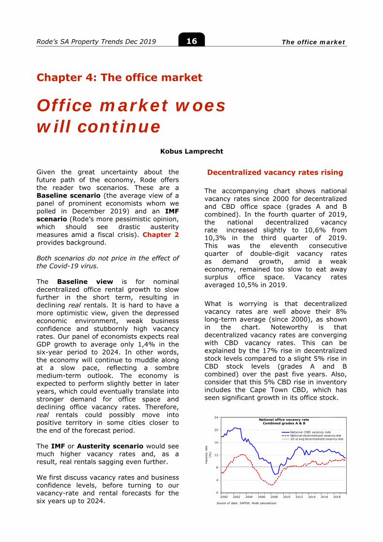
The accompanying chart shows national vacancy rates since 2000 for decentralized and CBD office space (grades A and B combined). In the fourth quarter of 2019, the national decentralized vacancy rate increased slightly to 10,6% from 10,3% in the third quarter of 2019. This was the eleventh consecutive quarter of double-digit vacancy rates as demand growth, amid a weak economy, remained too slow to eat away surplus office space. Vacancy rates averaged 10,5% in 2019.

What is worrying is that decentralized vacancy rates are well above their 8% long-term average (since 2000), as shown in the chart. Noteworthy is that decentralized vacancy rates are converging with CBD vacancy rates. This can be explained by the 17% rise in decentralized stock levels compared to a slight 5% rise in CBD stock levels (grades A and B combined) over the past five years. Also, consider that this 5% CBD rise in inventory includes the Cape Town CBD, which has seen significant growth in its office stock.

0

4

8

12

16

20

24

2000 2002 2004 2006 2008 2010 2012 2014 2016 2018

National CBD vacancy rateNational decentralized vacancy rate20-yr avg decentralized vacancy rate

National office vacancy rateCombined grades A & B

Vac

ancy

rat

e(%

)

Source of data: SAPOA; Rode calculations


Apropos, a long-term vacancy rate of grades A and B combined of 8% has an important implication when valuing prime office buildings. It is dead wrong to assume that even if an office building is near fully let at the time of valuation, this will persist in perpetuity.

The biggest improvement in vacancy rates came from the Pretoria CBD (3,1% compared with 13,6%) and Johannesburg CBD (10,9% compared with 13,3%), while Cape Town only saw a small decrease because of its strong growth in supply. Johannesburg CBD office stock declined by 4% compared to five years ago due to almost no new space being constructed and some office space being converted to residential space. The vacancy rate of the Durban CBD is the worst of all the major CBDs at 20,8% − a sharp deterioration from 14% five years ago.

Low business confidence

In the fourth quarter of 2019, only 26% of respondents surveyed by the BER were satisfied with prevailing business conditions. This is somewhat higher than the 21% in the previous quarter, which was a 20-year low. Firms are, therefore, likely to be hesitant to expand their premises or hire new employees. In fact, many companies are reducing their office space and the number of employees. This will keep office vacancy rates elevated for the next few years. Rode’s forecasts of vacancy rates and rental growth per scenario are discussed and shown in the charts and tables that follow.

Baseline scenario

a) Decentralized and CBD vacancyrates to increase in the short term, then decline Vacancy rates of all the major decentralized cities weakened in 2019, except for Pretoria, as shown in the chart. Under the Baseline scenario, we expect national decentralized vacancy rates to generally be higher in 2020 as economic growth remains too weak to curb the current oversupply (see Table 4.1).

Vacancy rates would improve gradually from about 2021 as economic growth starts to lift more meaningfully. Of course, such a relatively positive scenario assumes the land expropriation issue will be handled in a statesmanlike fashion, thus not having a big impact on the economy and property.

Decentralized vacancy rates should remain the highest in Johannesburg and Pretoria due to the current significant oversupply, but we do expect these to improve somewhat over the medium term as economic growth picks up. Vacancy rates in Durban and Cape Town should continue to be the lowest.

2

4

6

8

10

12

14

16

90 92 94 96 98 00 02 04 06 08 10 12 14 16 18 20 22 24

JohannesburgPretoriaDurbanCape Town

Baseline scenarioDecentralized office vacancy rates

(Grades A & B combined)

Forecast

Source of data: SAPOA; Rode forecasts

% v

acan

cy

Durban decentralized office vacancy rates are currently under pressure, but the medium-term outlook is more promising as all the office space under construction was already pre-let at the end of 2019. Besides, only 10 000 m² space is under construction.

Still under the Baseline scenario, Cape Town decentralized office vacancy rates are expected to increase in 2020, but then to slowly decrease due to improving economic growth. Existing space under construction is only about a third pre-let, which poses a risk to near-term vacancy rates. However, the medium-term outlook is positive as the city should increasingly attract companies, even multinationals, due to its good lifestyle and passable service delivery, while the drought problem of previous years is also out of the way. Plans by Cape Town to obtain its own electricity supply independent of Eskom is positive for


longterm property rentals and values. We believe its economy should fare slightly better than the rest of the country.

0

5

10

15

20

25

30

90 92 94 96 98 00 02 04 06 08 10 12 14 16 18 20 22 24

PretoriaCape TownDurbanJohannesburg

Baseline scenarioCBD office vacancy rates(Grades A & B combined)

Forecast


% v

acan

cy

Our models show that vacancy rates of prime offices in the CBDs of the major cities will most likely also worsen at the beginning of the forecast period, before improving with economic growth. Vacancy rates in the CBDs of Durban and Johannesburg are expected to recover but remain in double digits. Johannesburg vacancy rates should continue to benefit from lower office stock levels due to residential conversion.

b) Decentralized and CBD rentals willstruggle in the short term

Worsening vacancy rates bode ill for decentralized market rentals over the next few years. Therefore, we forecast nominal rentals to generally grow at below the expected building-cost rate at first but pick up close to the end of the six-year forecast period as the decline in vacancies gathers pace in the wake of faster economic growth. Thus, real rental growth is still a few years away. The practical implication is that developments will become even less viable than at present.

The corresponding chart shows our forecast of real decentralized rentals. The trends in the different cities are roughly the inverse of the vacancy rates discussed above.

110

100

90

80

70

60

5000 02 04 06 08 10 12 14 16 18 20 22 24


Baseline scenarioReal decentralized office rentals

Nominal rentals deflated by the BER BCI (2016 = 100)

Forecast

Rea

l ren

tal i

ndic

es (

2000

= 1

00)


Growth in nominal market rentals in the CBDs of major cities is forecast to be generally below the expected growth of building costs (or replacement cost). As a result, we expect real rentals to head south over the forecast period. Cape Town could be the exception later in the period, as the economy of the Mother City is expected to recover faster than in the rest of South Africa, thereby leading to growing business confidence and expanding office demand.

200

160

120

80

4090 92 94 96 98 00 02 04 06 08 10 12 14 16 18 20 22 24


Baseline scenarioReal CBD office rentals


Forecast

Rea

l ren

tal i

ndic

es (

2000

= 1

00)


IMF scenario

If an IMF-type scenario materializes, decentralized vacancy rates would worsen much faster over the first few years, staging some recovery towards the end of the forecast period, as shown in the chart.


2

4

6

8

10

12

14

16

90 92 94 96 98 00 02 04 06 08 10 12 14 16 18 20 22 24


IMF scenarioDecentralized office vacancy rates

(Grades A & B combined)

Forecast


% v

acan

cy

Nominal rentals would struggle significantly more in the first few years of the forecast period, and only thereafter recover somewhat towards the end of the forecast period (Table 4.4). The IMF scenario forecast of real decentralized rentals is

shown in the accompanying chart. CBD rentals would also perform very poorly under such a scenario.

110

100

90

80

70

60

50

4000 02 04 06 08 10 12 14 16 18 20 22 24


IMF scenarioReal decentralized office rentals


Forecast

Rea

l ren

tal i

ndic

es (

2000

= 1

00)


Detailed forecasts are shown in Tables 4.1 to 4.4.


Forecast of grades A+, A & B office vacancies % vacant

2018 2019 2020 2021 2022 2023 2024 Avg: 19-24

Johannesburg CBD 14,2% 11,0% 11,4% 11,3% 11,1% 10,7% 10,2% 10,9% Johannesburg dec. 11,5% 12,0% 12,3% 11,9% 11,3% 10,4% 9,6% 11,2% Pretoria CBD 5,1% 3,1% 4,9% 6,4% 6,0% 5,6% 5,3% 5,2% Pretoria dec. 10,9% 10,1% 10,7% 10,4% 10,2% 9,8% 9,5% 10,1% Durban CBD 20,9% 21,8% 21,0% 19,3% 18,3% 16,1% 14,6% 18,5% Durban dec. 7,5% 8,2% 8,4% 7,3% 6,5% 5,9% 5,7% 7,0% Cape Town CBD 10,6% 10,6% 10,3% 10,6% 9,9% 8,9% 7,7% 9,7% Cape Town dec. 4,4% 5,0% 5,3% 5,2% 4,8% 4,5% 4,2% 4,8%



Forecast of nominal prime office rentals % change on previous year

2018 2019 2020 2021 2022 2023 2024 Avg: 19-24

National: dec (weighted)

4,1% 4,1% 1,5% 3,0% 5,0% 7,1% 8,8% 4,9%

Johannesburg CBD 13,1% -10,4% 3,5% 4,0% 4,9% 6,0% 6,4% 2,4% Johannesburg dec. 4,1% 1,5% 0,6% 2,7% 5,3% 7,5% 9,5% 4,5% Pretoria CBD -1,1% 0,6% 2,3% 1,4% 3,6% 5,6% 7,4% 3,5% Pretoria dec. 3,1% 9,8% 2,0% 3,0% 3,8% 5,3% 6,0% 5,0% Durban CBD 17,0% 2,5% 3,0% 3,7% 4,4% 5,5% 6,4% 4,2% Durban dec. 0,9% 3,7% 2,5% 2,8% 4,0% 6,9% 8,8% 4,8% Cape Town CBD 6,8% 3,3% 3,6% 2,8% 5,9% 8,3% 9,4% 5,5% Cape Town dec. 8,1% 6,1% 4,9% 4,7% 6,4% 9,1% 11,0% 7,0%


Forecast of real prime office rentals % change on previous year

Series deflated using BER BCI

2018 2019 2020 2021 2022 2023 2024 Avg: 19-24

National: dec. -3,5% -0,9% -4,0% -3,7% -2,6% -0,9% 0,2% -2,0% Johannesburg CBD 4,7% -14,7% -2,1% -2,8% -2,6% -2,0% -2,0% -4,4% Johannesburg dec. -3,6% -3,3% -4,9% -4,0% -2,3% -0,6% 0,8% -2,4% Pretoria CBD -8,4% -4,2% -3,3% -5,2% -3,8% -2,4% -1,1% -3,3% Pretoria dec. -4,5% 4,6% -3,6% -3,7% -3,7% -2,7% -2,4% -1,9% Durban CBD 8,3% -2,4% -2,6% -3,0% -3,1% -2,4% -2,1% -2,6% Durban dec. -6,6% -1,2% -3,1% -3,9% -3,5% -1,2% 0,2% -2,1% Cape Town CBD -1,1% -1,7% -2,1% -3,9% -1,7% 0,1% 0,7% -1,4% Cape Town dec. 0,1% 1,0% -0,8% -2,1% -1,2% 0,8% 2,2% 0,0%

Using building costs as a deflator allows the reader to interpret the graphs from a developer’s point of view, i.e. the deflated rentals serve as a proxy for the viability of new developments over time, holding constant capitalization rates and operating costs.



Forecast of nominal prime office rentals % change on previous year

2018 2019 2020 2021 2022 2023 2024 Avg: 19-24

National: dec (weighted)

4,1% 4,1% 0,8% -1,4% 1,6% 3,0% 4,7% 2,1%

Johannesburg dec. 4,1% 1,5% 0,2% -1,2% 1,7% 2,9% 5,1% 1,7% Pretoria dec. 3,1% 9,8% 1,3% -2,4% 1,5% 2,8% 3,2% 2,7% Durban dec. 0,9% 3,7% 1,2% -1,4% 1,7% 3,2% 4,7% 2,2% Cape Town dec. 8,1% 6,1% 3,1% -0,8% 1,2% 3,6% 5,7% 3,1%

In sum …

The office market is still overwhelmed by oversupply. Under the Baseline scenario, this would keep nominal rental growth below building-cost inflation for the next few years amid very slow economic growth. However, we do expect nominal decentralized office rental growth to accelerate closer to the end of the six-year forecast period as a pick-up in economic growth leads to declining vacancy rates. Therefore, real rental growth is likely only towards the latter part of the six-year forecast period.

The IMF scenario, to which we assign a higher probability of 60%, would see much higher vacancy rates and, as a result, real rentals would sag even further.

In the major CBDs, except maybe Cape Town, real rentals are likely to decline over the entire forecast period.

Note that the above forecasts are premised on the assumption that SA will not end up with precarious property tenure. It also assumes away the potential impact of the Covid-19 virus.

Rode’s SA Property Trends Dec 2019 The industrial market 22

Chapter 5: The industrial market

Industrial market cools Kobus Lamprecht

Given the great uncertainty about the future path of the economy, we offer the reader two scenarios. These are a Baseline scenario (the average view of a panel of prominent economists whom we polled in December 2019) and an IMF scenario (Rode’s more pessimistic opinion, which should see drastic austerity measures amid a fiscal crisis). The tag ‘IMF scenario’ might as well be ‘Austerity scenario’ because SA will have the choice of doing the dirty deed itself or having it imposed via the IMF. Chapter 2 provides background.

Note that both scenarios do not price in the effect of the Covid-19 virus.

The industrial market cooled in 2019, with nominal rental growth slowing compared to 2018 due to the weakening manufacturing and retail sectors. Under the Baseline scenario, we expect rentals to decelerate over the next two years or so due to continued subdued economic growth, which would impact the demand for warehousing. The outlook for the latter part of the six-year forecast is more promising with faster nominal rental growth expected, which could lead to real rental growth in some industrial conurbations. The IMF scenario would see much higher vacancy rates and, as a result, real rentals sagging even further.

Below we first discuss the recent rental performance of industrial property, before analysing the major factors impacting the market. Lastly, we provide forecasts for vacancy rates and market rentals in the metros over the next six years.

Latest rentals cool

Nominal industrial market rentals in South Africa grew by 5,7% in 2019, slowing from the 6,3% growth recorded in 2018. Despite this cooling, rentals still managed to grow in real terms, after adjusting for building-cost inflation (BER BCI) of about 5%. On a quarterly basis, rental growth (4%) was the slowest in the fourth quarter of last year, perhaps as the weaker performance of the manufacturing and retail sectors is finally taking its toll.

Changes in rentals and vacancy rates are strongly linked to the performance of the manufacturing and retail sectors, as well as business confidence levels. The manufacturing sector underpins the demand for industrial space for manufacturing production and warehousing purposes, whereas the retail sector underpins the demand for warehouse space and manufacturing.

In 2019 the manufacturing sector performed worse than in 2018, with Stats SA data showing production fell by 0,9%. The sector is facing numerous challenges, most notably interruptions in power supply. Worryingly, at the end of January 2020 Eskom said that the country should brace itself for more frequent power cuts over the next 18 months as the power utility steps up maintenance on its power stations. The Absa Purchasing Managers’ Index (PMI)1 shown in the chart was also mostly below 50 in 2019 and fell to 44,3 points in February this year, the weakest level since the second half of 2009. Note that when the PMI is below 50 points it is an indication that the manufacturing sector is

1 Compiled by the BER at Stellenbosch University


in contraction territory.

36

40

44

48

52

56

60

06 07 08 09 10 11 12 13 14 15 16 17 18 19 20

Expansion

Contraction

Inde

x

Source of data: BER; ABSA

ABSA Purchasing Managers' Index(Seasonally adjusted)

As for the longer term, it is evident in the graph that we have had a declining trend since the peak of 2007, with a sudden accelerated slide in 2019. Put differently, over time fewer of the yellow bars have been above the neutral line of 50. This is consistent with a South Africa that is deindustrialising, like a true First World country – as if we can afford this. The fact remains that the SA manufacturing sector is uncompetitive internationally on many fronts, especially on labour costs and productivity, which will not change any time soon. This will remain a deterrent to growing production, influencing the demand for industrial space and ultimately holding back rental growth. Besides, who would want to invest if you do not have electricity?

As the saying goes, how does a company (country) go bankrupt? At first slowly, then suddenly.

The retail sector is also struggling, with real sales for 2019 up only 1,2% due to subdued consumer spending. This growth rate is slower than the 2,2% rate achieved for the full 2018. In fact, it is the worst annual performance since 2009. So, we are seeing a slowdown in sales growth in tandem with a slowing economy (see Chapter 6).

A positive for the industrial market is the ever-growing demand for new-generation warehouse or distribution space due to the significant growth of online retail sales – albeit from a low base. Online retail grew

by 25% in 2018 to make up 1,4% of total retail sales, according to the findings of World Wide Worx’s Online Retail in South Africa 2019 study. Modern racking systems make stacking heights of more than 12 metres possible, thus requiring a new generation of warehouses. This has the potential of making many existing distribution centres outdated.

Another factor to consider is changes in business confidence, as measured by the RMB/BER Business Confidence Index. The corresponding graph shows the strong inverse correlation between industrial property vacancies (national) and business confidence. Naturally, business decision makers can be expected to be hesitant to expand production capacity or storage space by renting more space when they are dissatisfied with prevailing business conditions. The “r²=0,7” shown in the graph implies that about 70% of the change in industrial property vacancies can be explained by changes in business confidence levels, with a lag of about one year. However, if one were to include additional determinants of vacancies in a regression model, this correlation would be lower.

1.2

1.6

2.0

2.4

2.8

3.2

3.6

0

20

40

60

80

100

90 92 94 96 98 00 02 04 06 08 10 12 14 16 18

Vacancy factorBusiness confidence

Rode's industrial vacancy factor (national)vs

RMB/BER Business Confidence Index

Vac

ancy

sca

le(1

-9)

r² = 0,7 (4-quarter lag)

Business

Confidence

Index

Source of data: Rode's Time Series; BER

smoothed

The national vacancy factor increased to about 2,5 points in the fourth quarter of 2019, the worst level of the year, likely as consistently weak business confidence is impacting negatively on firms’ decision to expand production capacity or storage space. However, 2,5 points is still considered ‘low’ on Rode’s vacancy scale of 1-9, implying that less than 5% of industrial property was vacant at the time.


Therefore, we are seeing weakening vacancy rates from a low level.

In the fourth quarter of 2019, only 26% of respondents surveyed by the BER were satisfied with prevailing business conditions. The implication is that continued low business confidence could result in increasing industrial vacancies over the next year or so.

The higher vacancy rates led to weaker market rental growth of 4% in the fourth quarter of 2019 compared to a 6,3% average in the previous quarters of the year, as can be seen in the chart.

-10

0

10

20

30

1.2

1.6

2.0

2.4

2.8

3.2

3.6

92 94 96 98 00 02 04 06 08 10 12 14 16 18

RentalsVacancy factors

Change in prime industrial rentalsvs

Industrial property vacanciesNational

r²=0,4

Vacancy

scale(1-9)

Cha

nge

in r

enta

ls(%

; y-

o-y)

Source of data: Rode's Time Series

smoothed

Rode’s forecasts of vacancy rates and rentals are discussed and shown in the charts and tables that follow.

Baseline scenario – vacancy rates will worsen over the next year or two

As for our forecasts, in terms of the Baseline scenario, our panel of economists expects real GDP growth to improve gradually over the six-year forecast period but averaging only 1,4%. Growth is expected to be meagre at the start of the period, which would continue to weigh on business sentiment and the manufacturing and retail sectors. Only from about 2021/22, as economic growth picks up more meaningfully, would a decline in vacancies result, as shown in the chart.

The Cape Peninsula should continue to stand out with the lowest vacancy rate of the major industrial conurbations. Plans by

Cape Town to obtain its own electricity supply independent of Eskom is positive for long-term property rentals and values.

1.0

1.5

2.0

2.5

3.0

3.5

4.0

4.5

00 02 04 06 08 10 12 14 16 18 20 22 24

Central WitwatersrandDurbanCape PeninsulaPort Elizabeth

Baseline scenarioIndustrial vacancies


Vac

ancy

sca

le (

1 -

9)

Forecast

1.0

1.5

2.0

2.5

3.0

3.5

4.0

4.5

00 02 04 06 08 10 12 14 16 18 20 22 24

Central WitwatersrandDurbanCape PeninsulaPort Elizabeth

IMF scenarioIndustrial vacancies


Vac

ancy

sca

le (

1 -

9)

Forecast

If an IMF-type scenario materializes, vacancy rates would worsen much faster at the beginning of the period, staging some recovery towards the end of the forecast period, as shown in the chart.

Baseline scenario – rentals will slow at first, but then perform better

Nominal rentals generally beat inflation in 2019 but should slow down in 2020 and 2021 owing to rising vacancy rates as a result of sustained weak performances by the manufacturing and retail sectors. Therefore, we expect real rentals to head south as shown in the chart. The decline in vacancies later in the six-year period would augur well for nominal market rentals. In fact, we expect real industrial rentals to turn positive in some industrial conurbations, like the Cape Peninsula.


110

100

90

80

70

6000 02 04 06 08 10 12 14 16 18 20 22 24

Port ElizabethCape PeninsulaDurbanCentral Wits

Baseline scenarioReal industrial rentals:

(500m² units)

Rea

l ren

tal i

ndic

es (

2000

= 1

00)

Source of data: Rode's Time Series; BER; MFA

Deflated by BER BCI (2016 = 100)

Forecast

If the IMF scenario plays out, nominal rentals would significantly struggle more, especially in 2020 and 2021, as vacancy rates are expected to be much higher compared to the Baseline scenario. We expect real rentals to generally be in negative territory for the entire forecast

period, as can be seen in the accompanying chart.

110

100

90

80

70

6000 02 04 06 08 10 12 14 16 18 20 22 24

Port ElizabethCape PeninsulaDurbanCentral Wits

IMF scenarioReal industrial rentals:

(500m² units)

Rea

l ren

tal i

ndic

es (

2000

= 1

00)

Source of data: Rode's Time Series; BER; MFA

Deflated by BER BCI (2016 = 100)

Forecast

Our forecasts of industrial vacancies and rental growth are summarized in Tables 5.1 to 5.4.


Forecast of industrial vacancy factors (on a vacancy scale of 1-9; these are not vacancy percentages*)

Average for the year

2018 2019 2020 2021 2022 2023 2024 Avg 19-24

Central Wits 2,38 2,42 2,75 2,75 2,73 2,69 2,63 2,66 Greater Durban 2,46 2,88 3,06 3,07 3,00 2,94 2,88 2,97 Cape Peninsula 2,12 2,02 2,33 2,23 2,12 2,00 1,94 2,11 Port Elizabeth 3,59 3,28 3,71 3,61 3,52 3,32 3,20 3,44 *Rode asked its industrial survey panel to rate the level of industrial property vacancies in an industrial township ona scale from 1 to 9, where 1 – 3 = ‘low’ vacancy (<5%); 4 – 6 = ‘medium’ vacancy (5% - 10%); 7 – 9 = ‘high’ vacancy (>10%).

Some history: secular decline in industrial property rentals

Since the early 1980s, the South African manufacturing industry has been hard hit by several factors. At different times, different factors have played a role, but here are some of the more prominent reasons (in no specific order):

Deteriorating workforce productivity (output relative to fast-rising wages from the 1980sonwards)

Low economic growth (owing to, inter alia, sanctions, declining real commodity prices, high realinterest rates to combat inflation from 1989 onwards, political instability), resulting in feebledomestic demand

Reduction of trade tariffs in the 1990s Space-saving technological advances by the industry (which were good for manufacturers and

distributors but bad for property) Structural swing towards the services sector (in the developed world)


Dwindling contribution of the mining industry, caused by the weakening of hard-commodityprices, physical reasons (escalating deep-mining costs and depleting gold-mining reserves), andgovernment interventions in the mining industry

Latterly, the emergence of cheap-labour economies such as China and India.

The result: a secular decline in real industrial property rentals.


Forecast of nominal prime industrial rentals % change on previous year

2018 2019 2020 2021 2022 2023 2024 Avg: 19-24

Central Wits 6,7 7,3 2,5 2,8 4,6 6,1 7,4 5,1 Durban & environs 6,3 6,2 2,2 2,0 5,1 6,1 6,8 4,7 Cape Peninsula 13,4 5,8 4,2 5,3 7,6 9,3 10,8 7,2 Port Elizabeth 7,3 3,9 1,4 2,5 4,0 5,0 5,8 3,8


Forecast of real prime industrial rentals % change on previous year

Series deflated using BER BCI

2018 2019 2020 2021 2022 2023 2024 Avg: 19-24

Central Wits -1,2 2,2 -3,1 -3,9 -2,9 -1,8 -1,1 -1,8 Durban & environs -1,6 1,1 -3,4 -4,6 -2,4 -1,9 -1,6 -2,1 Cape Peninsula 5,0 0,7 -1,4 -1,6 -0,1 1,1 2,1 0,1 Port Elizabeth -0,7 -1,0 -4,1 -4,2 -3,5 -2,9 -2,6 -3,1

By using building costs as a deflator, the reader can interpret the graphs from a developer’s point of view, i.e. they can serve as a proxy for the viability of new developments over time, holding constant capitalization rates, operating expenses and demand for space.


Forecast of nominal prime industrial rentals % change on previous year

2018 2019 2020 2021 2022 2023 2024 Avg: 19-24

Central Wits 6,7 7,3 -2,3 2,6 3,2 4,5 6,1 3,6 Durban & environs 6,3 6,2 -1,9 2,3 3,0 3,4 4,0 2,8 Cape Peninsula 13,4 5,8 2,2 1,2 3,7 6,0 9,0 4,6 Port Elizabeth 7,3 3,9 -3,6 1,8 2,3 2,8 3,8 1,8


In sum …

The performance of industrial rentals will depend on the performance of its support pillars, namely the manufacturing and retail sectors. In terms of the Baseline scenario (p=40%), our panel of economists expects economic growth to be meagre over the next few years, but then to grow more meaningfully later in the forecast period. This implies that nominal rental growth in the country’s major industrial conurbations will first head south, before starting to pick up in the latter part of the forecast period. Real rentals should

be in negative territory for most the forecast period. Under the IMF scenario (p=60%) things will get much worse.

Beware of speculative developments – the uncertainty is just too great.

Note that the above forecasts are premised on the assumption that SA will not end up with precarious property tenure. In addition, neither of these scenarios prices in Covid-19’s effect on the global and South African economy. So, the reader should, for planning purposes, assume the above scenarios are optimistic.

Rode's SA Property Trends Dec 2019 Retail property 28

Chapter 6: Retail property

Retail sales growth slows to 10-year low

Kobus Lamprecht

This chapter does not cover any quantitative retail property forecasts, as the retail property market is too heterogeneous (mall and location specific) for such details. We do, however, sketch a qualitative prognosis by considering factors that are likely to impact on demand and supply up to 2024.

Prognosis for retail sales

Landlords in the retail property sector generally struggled in 2019 due to high vacancy rates amid an oversupply of space and weak growth in retail sales. Mall vacancy rates could lift even more as retailers are under severe pressure, with several companies closing stores. In early 2020 Massmart, the owner of Game and Makro, announced plans to close 34 Masscash and DionWired stores. This comes after the Edcon group shut 150 stores last year. The closure of bank branches is also leading to more vacant space. The introduction of foreign retailers over the past few years is probably one of the contributing reasons why retailers are struggling.

Retail sales grew by 1,2% in real terms in 2019 – growth-wise a 10-year low – as households are feeling the heat on many fronts, notably poor employment growth (read: shedding of jobs) and the rising cost of living. Lower interest rates should bring some relief in the near term, but this will be offset by the negative factors. Given the huge structural and policy ‘challenges’ facing SA, it is not clear how lower interest rates are going to benefit SA in the long

term. Overindebted consumers maybe buying more on the never-never?

A positive is the continued increase in nominal trading densities (sales/m²) of malls. This implies that malls are outperforming the overall retail market. However, expenditure per mall visitor – a significant driver of trading-density growth – is slowing down, according to the latestSAPOA data.

On the supply side, the market is still under pressure from too much shopping space. A positive for the sector’s prospects is that new supply is likely to be significantly less in the coming years. This implies the market has the potential to be on a better footing in a few years. Well, that is if the economy also plays ball to give sales a strong boost, which is unlikely, given the Baseline scenario forecast of GDP growth of 1,4% over the six-year period ending 2024. The prospects for retail sales are even worse if the IMF scenario materialises.

In this article, we first focus on the demand for merchandise by analysing the ability of consumers to spend. We also delve deeper into the latest retail sales statistics and trading densities for malls. Lastly, the supply of new shopping centre space is considered.

Sales

Spending by consumers or households is related to their disposable income relative to inflation and access to credit.


Real expenditure of households increased by only 1,1% in the first nine months of 2019 compared to the same period in 2018. This measure moderated to 0,2% in the third quarter of 2019 due to slower disposable income growth and depressed consumer confidence. The latter was at a two-year low in the fourth quarter of 2019. Some of the factors putting pressure on household finances are poor employment growth and the rising cost of living (think growing housing rentals/house prices, electricity tariffs, medical scheme fees, school fees and fuel).

In the meantime, household expenditure is still being supported by credit growth. Real credit extended to households (dotted line in the graph below) in 2019 increased by 3,7%, up from the 2,8% pace recorded in 2018. However, the National Credit Amendment Bill signed into law in August 2019 could slow credit growth through tighter lending standards and the higher cost of credit. This means retailers and banks will likely charge low-income consumers a substantial interest rate premium compared to the prime rate to protect them from non-payment (the prime rate was lowered to 9,75% from 10% in January 2020). While this is not good news for retailers in the short term, in the long run greater financial discipline should be welcomed.

A coefficient of determination (r²) of 0,6 in the graph means that up to 60% of the changes in real retail sales are explained by changes in real credit extended to households, without controlling for other independent variables such as interest rates, inflation and disposable incomes. Note how a recovery in debt extension held

up spending during the past two years. Do we really want to increase debt-based spending through lower interest rates?

-8

-4

0

4

8

12

16

20

24

28

03 04 05 06 07 08 09 10 11 12 13 14 15 16 17 18 19

Retail salesloans to households

Change in real retail salesvs

Change in real credit extended to households

Cha

nge

(%;

y-o-

y)

Source of data: Stats SA; SARB

r²=0,6 Nominal values deflated by the retail price deflator

Retail sales grew by 1,2% in real terms in 2019 as shown in Table 6.1. This growth rate is slower than the 2,2% rate achieved for the full 2018. In fact, it is the worst annual performance since 2009. So, we are seeing a slowdown in sales growth in tandem with a slowing economy.

A closer look at the trends in real sales in Table 6.1 reveals mostly slow growth across most retailer types. General dealers (about 42% weight in total sales) recorded sales growth of 1,1%. Retailers of household furniture, appliances & equipment (+2,8%) had the strongest increase of all categories, boosted by lower prices compared to 2018.

Retailer inflation averaged 2,6% in 2019, up from 2018’s 1,7%, but still lower than headline or general inflation of 4,1%. However, low inflation has not really translated into stronger retail sales growth, implying that consumers are under too much financial pressure to lift purchases.


Table 6.1 Real retail sales by type of retailer

Jan-Dec 2019 compared to Jan-Dec 2018

Retailer type Growth in real sales

Change in price deflator*

General dealers 1,1% 3,6%Food, beverages & tobacco in specialised stores 0,8% 3,5%Pharmaceutical & medical goods, cosmetics & toiletries 1,3% 5,3%Textiles, clothing, footwear & leather goods 1,8% 1,0%Household furniture, appliances & equipment 2,8% -1,2%Hardware, paint & glass -1,5% 2,9%All other retailers 1,8% -0,3%Total 1,2% 2,6%*The yearly growth in the price deflators (2015 prices) used to deflate nominal retail sales figures, in other words,inflation. †All ‘other’ retailers are retailers in reading matter and stationery; retailers in jewellery, watches and clocks; retailers in sports goods and entertainment requisites; retailers in ‘Other’ specialised stores; repair of personal and household goods; retail trade in second-hand goods in stores; and retail trade not in stores. Source: Stats SA

Retail sales growth is likely to remain slow in the near term due to generally poor household finances and low consumer confidence. Nevertheless, we still believe sales growth will remain in positive territory, boosted by credit purchases, slightly lower interest rates and low inflation.

Over the medium term the sales outlook is poor, given the Baseline scenario forecast of GDP growth of 1,4% over the six-year period ending 2024. The outlook for the IMF scenario is even worse.

Trading densities in malls

Nominal trading densities (sales/m²) in malls increased by 4,3% in the 12 months to September 2019 compared to the previous 12 months (see the chart on the next page), according to MSCI Real Estate, published in the SAPOA Retail Trends Report. This is up slightly from a revised 4,1% in the year to June 2019. Thus, trading densities are continuing to grow in real terms, after adjusting for retail inflation (which, as per Table 6.1, is much lower than the general inflation as

measured by the CPI). In interpreting the graph, note that while the line representing changes in nominal sales is below the zero line, sales per m² are contracting, though the pace of contraction varies.

The 4,3% nominal trading-density increase comprised a 5,5% increase in total sales, while the occupied trading area rose by 1,2%. Nominal sales growth of the overall retail market was 3,6% in the year ended September 2019, implying that MSCI’s sample of mall-based retailers outperformed the overall retail market.

Delving deeper into MSCI’s data reveals that foot count/m² increased by 2,5% ̶ this measure has now grown every month since April 2019. However, expenditure per consumer increased by 1,7% – the lowest growth rate since the end of 2015. Thus, shoppers are visiting malls more, but not maintaining their spend per visit. Maybe they are buying the proverbial lipstick. 1 Other statistics generally point to malls still being under pressure. For example, the vacancy rate of malls was still high at 4,4% in the third quarter, above its long-term average of 2,9%.

1 A widely held belief is that during tough times women who are out of money would as a morale booster buy small items like lipstick.


Table 6.2 shows the change in trading densities for the 12 months to September 2019, as well as the latest vacancy rate by retailer type. It is clear from the table that the growth in trading densities was driven mostly by neighbourhood and community centres, which recorded above-inflation trading-density growth of 9% and 5,1% respectively. The larger centres, especially regional centres, seem to be struggling the most, with trading-density growth averaging between 1% and 3%. In judging

these growth rates, consider that the retail inflation (Table 6.1) clocked only 2,6%.

Table 6.3 below provides more detail by showing the change in trading densities by merchandise category for the 12 months to September 2019. Electronics (+8,3%) recorded the best growth, followed by Food (+7,2%) and Department stores (+6,8%). Apparel shops managed trading-density growth of only 1,7%. Note, these are nominal growth rates.

Table 6.2 Vacancy rates and nominal y-o-y change in trading densities

12 months to Sept 2019

Retailer type Change in trading densities in nominal terms (%)*

Vacancy rate (%)**

Super Regional 2,6 4,7 Regional 1,1 3,2 Small Regional 2,7 4,9 Community 5,1 3,8 Neighbourhood 9,0 5,5 Total 4,3 4,4 *12 months to Sept 2019**As at third quarter 2019 Source: MSCI Real Estate; SAPOA


Table 6.3 Nominal change in trading densities (%)

For top five merchandise categories 12 months to Sept 2019 Merchandise category % change in trading density

Electronics 8,3 Food Services* 4,8 Food 7,2Dept Stores 6,8 Apparel 1,7Total (all merchandise categories) 4,3 *Food services include restaurants and fast-food outlets.Source: MSCI Real Estate; SAPOA

Table 6.4 New shopping centre completions (m²)

Excluding refurbishments and minor extensions to centres smaller than 5.000 m²

2017 2018 2019* 2020*#Cape Peninsula 68.000 10.400 49.140 7.500 Reef 146.082 39.400 134.563 82.000 Pretoria 15.433 100.324 70.396 53.500 Durban 39.000 6.000 0 0Pietermaritzburg 0 22.000 0 0Port Elizabeth 0 0 0 0Nelspruit 0 18.000 0 0Polokwane 0 0 0 0Bloemfontein 0 0 6.000 0Kimberley 0 0 0 0Cities 268.515 196.124 260.099 143.000 Smaller towns/rural areas in:

Eastern Cape 0 0 4.452 0Free State 0 0 14.600 10.800 KwaZulu-Natal 141.000 30.292 25.167 2.500 Limpopo 126.500 53.751 64.000 12.460 Mpumalanga 62.000 68.188 40.584 11.200 Northern Cape 0 0 0 0Vaal Triangle 0 0 12.500 0North West 0 7.900 0 0Western Cape 28.000 0 0 0

Smaller towns/rural areas 352.500 160.131 161.303 36.960 Total 602.015 356.255 421.402 179.960 * Estimated# 2020 data only includes centres where construction has started Source: Rode's Shopping Centre Database


Supply of new shopping centre space

As for the supply side of the retail property market, Table 6.4 shows a breakdown by year and by geographic area of new shopping centre completions larger than 5 000 m², including major extensions.

Completions of new malls countrywide increased sharply in 2019, a turnaround from 2018’s sharp fall, according to Rode’s calculations. Most new space was in Gauteng, such as the Fourways Mall (extension of 90 000 m²) and the Tshwane Regional Mall (60 000 m²) in Mamelodi. What this trend illustrates is that mall completions are a lagging indicator of the economy.

We expect completions to fall significantly in 2020, given the low number of centres already under construction. Developers are also significantly scaling back their medium-term building plans, which is not surprising given the weak economic outlook and oversupply. Thus, building plans

passed for shopping centres in 2019 declined by 10%, according to Stats SA. This will surely be a relief for landlords of existing shopping centres, given the challenges facing the sector.

In sum …

Retail sales in the overall retail market are still growing at a slow pace amid weak consumer spending, even with low price increases. This is not surprising as households remain under severe financial pressure.

The medium-term outlook for the economy, and sales in general, is bleak. Thus, peering into the future, the golden years of malls are evidently over for quite a few years. But then, this applies to the economy in general and, therefore, to just about all investment channels.

On the supply side, the market is still under pressure from too much shopping space. A positive for the sector’s prospects is that new supply is likely to be significantly less in the coming years.

Rode’s SA Property Trends Dec 2019 The residential market

Our review of prospects for the residential property market includes forecasts of house prices and flat rentals for South Africa. The house price movements are based on house price indices by Absa (historical data) and FNB, while the flat–rental movements are based on Rode’s Flat Rental Index (all sizes; standard units) and Stats SA.

The forecasts in this chapter are exclusively based on the Baseline scenario. The IMF scenario would of course result in much worse outcomes.

Chapter 7: The residential market

House prices still battling to beat inflation

Kobus Lamprecht

The residential market remains under pressure, with nominal house price growth slowing for the fifth consecutive year in 2019. National house prices as measured by FNB grew by 3,6% in nominal terms in 2019, in line with our projection in Trends June 2019. This implies that prices have continued to decline in real terms (after having taken out inflation – whether measured by the BER Building Cost Index or the CPI). The market is still slightly oversupplied, most significantly in the high end of the market. The very-low end of the market is looking healthier, with strong price growth and lower vacancies.

Below we first discuss the drivers of house prices, followed by our forecasts for house prices and flat rentals.

Drivers of changes in house prices

House prices correlate well with the value of residential mortgages granted over the long term, with r² = 0,5, as shown in the chart and explained in more detail in the text that follows. The nominal value of residential mortgages granted in the first nine months of 2019 picked up by 9% year on year, after an 18% surge in the third quarter (see sharp jump in the chart).

-20

-10

0

10

20

30

40

50

-60

-40

-20

0

20

40

60

80

2002 2004 2006 2008 2010 2012 2014 2016 2018

House pricesMortgage loans (smoothed)

Change

innew

mortgage loans

(%; y-o-y)

Cha

nge

in h

ouse

price

s(%

; y-

o-y)

Change in national house prices (FNB)vs

Change in value of new mortgage loans

Source of data: FNB; SARB

r²=0,5

Because of all the economic headwinds, the lift in mortgages granted has not really manifested in accelerated house price growth as seen in the chart. Overall, house price growth remained relatively stable between 3% and 4% in the second half of 2019. Thus, our view is that the relaxed credit criteria are preventing the market from weakening further (holding all other factors constant). It is worth considering the mechanism that creates the relationship between house prices and the value of mortgages granted, which is probably twofold:

As house prices increase, the value of mortgages will rise − provided banks keep their loan-to-value policies constant. This would mean that house prices determine

34


the value of mortgages granted, not the other way around.

On the other hand, an increase in the value of mortgages granted could mean banks have relaxed their credit criteria (loan-to-price policies), which allows prices to accelerate and could, in addition, lead to more sales being concluded (holding all other factors constant). This would also result in more mortgage bonds being registered. In this instance, one could argue that the determinant of house prices is not the value of mortgage bonds registered but rather the change in banks’ credit policies.

This is where South Africa is: We know mortgagees (banks) are relaxing their loan-to-price policies, which – at least temporarily – is supporting house price growth. The loan-to-price (LTP) ratio has gradually increased over the past two years. It reached 91,2% in the third quarter of 2019, up from 90,6% in the second quarter of 2019, according to FNB. This suggests that lenders are progressively asking for smaller deposits from prospective buyers amid strong competition to gain new home-loan business. Loans are also being granted at more favourable interest rates – statistics from bond originator Ooba show that its average achieved interest rate for home buyers in the fourth quarter of 2019 was 13 basis points lower than a year earlier. In any case, the acceleration in mortgages granted is not sustainable − as explained later − as mortgage lenders (mortgagees) face huge short- to medium-term risks owing to the economy’s precarious state.

A significantly correlated variable of residential mortgages granted is the leading business cycle indicator of the SARB, with r² = 0,5. This indicator reflects early stirrings in the economy, thus confirming that the fundamental driver of house prices is the economy. This indicator fell by 1% in November 2019 compared to November 2018 and has been in negative territory for more than a year. This is not a good signal for the housing market.

-80

-40

0

40

80

120

-20

-10

0

10

20

30

98 00 02 04 06 08 10 12 14 16 18

Mortgage loans (smoothed)Business cycle leading indicator

Change in value of new residential mortgages grantedvs

Change in composite business cycle leading indicator

Cha

nge

in v

alue

of

mor

tgag

es g

rant

ed(%

; y-

o-y)

Change in business cycle indicator

(%; y-o-y)

Source of data: SARB

r²=0,5

In the medium term, we expect the growth in the value of mortgages granted to be slow as effective demand1 from borrowers will be impeded by several factors:

1) Continued slow economic growth.The economy grew at an averageannual rate of 1,4% in the six-yearperiod from 2013 and 2018. Interms of our Baseline scenario, ourpanellists expect growth to averagethe same rate in the six-yearforecast period from 2019 and2024. In other words, the economywill continue to muddle along at aslow pace – even in terms of ourbaseline scenario. Growth will behampered by cyclical factors (suchas the dire fiscal situation) andstructural problems (like the qualityof education and others we dare notmention). Additional issues that willweaken economic growth includecontinued electricity supplydisruptions/constraints and thesharp electricity price increases. TheEskom crisis cannot be solvedovernight.

2) In the current cycle, it is unlikelythat banks will relax their creditcriteria further in respect ofmortgage approvals. The reasonsare: The weak economy – see (1). The still-high ratio of household

debt-to-disposable income. Thisratio was at 72,6% in the third

1 Effective demand is a need the consumer can afford and is prepared to pay for.

35


quarter of 2019 ̶ up from 71,9% in the third quarter of 2018.

The prospects of rising unemployment in an overstretched economy. Jobprospects in the medium termare poor, given the subduedoutlook for economic growth andthe overpopulated SOEs andpublic sector.

Rising utility costs that erodedisposable incomes and thecompetitiveness of SA industry.Think electricity (Eskom is indire need of capital) and fuelprices (assuming the rand willweaken in the medium term).

A slight positive for the residential property market is the 25 basis-points cut in short-term interest rates in January 2020 (prime rate lowered to 9,75% from 10%), which follows the 25 basis-points reduction in July last year. However, don’t expect such small changes to turn the property market around. The interest rates were lowered to provide support to the economy and the cut was made possible by subdued local inflation and a worldwide trend of more accommodative monetary policy.

In terms of our Baseline scenario, Rode’s panel of economists expects local interest rates to remain largely stable for the rest of 2020. The prime interest rate should rise somewhat later in the forecast period, but on average stay close to 10%.

Be that as it may, fundamental/structural problems in the SA economy cannot be solved by interest rate tinkering. And the residential property market is inextricably linked to the economy.

Forecast of house prices and flat rentals (under the Baseline scenario)

We expect nominal house price growth to average 5% over the six-year forecast period from 2019 and 2024 (see

Table 7.1). Prices should be supported by slightly lower interest rates in 2020, but this impact would fade over the forecast period as interest rates pick up again. Prices should perform better each year, but no exceptional growth is expected as economic growth (as measured by real GDP) will generally remain slow (an average of 1,4%), with growth in the value of mortgages granted also subdued as a result. Thus, real house prices will decline as nominal prices grow at a slower rate than the increase in building costs (as measured by the BER BCI).

Flat rentals (Table 7.2) should also grow in nominal terms but decline slightly after adjusting for building-cost inflation. We expect flat rentals will perform somewhat better than house prices over the medium term as a result of the affordability factor (affordability will be compromised through poor growth in disposable incomes, rising unemployment and the possibility of banks tightening their credit policies in the light of the former two factors).

In sum ...

In terms of our Baseline scenario, we expect nominal house prices and flat rentals to pick up over the forecast period ending 2024, initially supported by lower interest rates. However, on average, prices will continue to decline in real terms due to a sharp rise in building costs (Chapter 9), thereby reducing the financial feasibility of residential developments. Thus, from the banks’ point of view, financing residential developments will become riskier, all other factors remaining constant. The greatest risk to residential developers is not profit margins but the tempo of sales (sales rate).

Note: In this chapter we forecast the residential property market assuming our Baseline scenario, which has a probability of 40%. Under our more pessimistic ‘IMF’ scenario (p=60%), the forecasts above would of course be worse. Neither scenario considers the potential impact of the Covid-19 virus on the world and SA economies.

36

Rode’s SA Property Trends Dec 2019 The residential market 37


Forecast of national house prices: % change on previous year

Nominal BER BCI deflated2018 3,8 -3,92019 3,6 -1,32020 3,9 -1,82021 4,5 -2,32022 5,5 -2,02023 6,0 -2,02024 6,6 -1,8Average: 2019-24 5,0 -1,9Source: Rode’s SA Property Trends, Dec 2019; Stats SA


Forecast of national flat rentals: % change on previous year

Nominal BER BCI deflated2019 5,3 -2,52019 4,4 -0,5 2020 3,8 -1,8 2021 5,1 -1,7 2022 6,5 -1,2 2023 7,2 -0,9 2024 7,6 -0,9 Average: 2019-24 5,8 -1,2Source: Rode’s SA Property Trends, Dec 2019; Stats SA

The forecasts in this publication are based on economic fundamentals and historical relationships. The econometric models’ forecasts assume that these relationships will continue.

Rode’s SA Property Trends Dec 2019 Capitalization and escalation rates 38

Chapter 8: Capitalization and escalation rates

Capitalization rates will worsen Kobus Lamprecht

Capitalization rates of directly held non-residential property in South Africa in the fourth quarter of 2019 continued to increase (deteriorate) from previous-quarter levels. We ascribe this to the poor ratings of listed funds and the weak outlook for the property market, including continued above-average vacancy rates and below-inflation rental growth.

Important disclaimer

The forecasts in this chapter do not price in the impact of the Covid-19 virus on the world and SA economies.

The respective national capitalization rates were 10% for prime multi-tenanted office properties, 9,5% for prime industrial leasebacks and 8,2% for regional shopping centres (see the chart). Note that all data series in this chapter are smoothed.

7

8

9

10

11

12

13

14

2000 2002 2004 2006 2008 2010 2012 2014 2016 2018

Regional shopping centresIndustrial leasebacksDecentralized offices

National capitalization ratesby property type


%

Smoothed

Rode’s view on future capitalization and escalation rates follows.

Cap rate outlook

Interest rates in general can affect the total returns (hurdle rates) and income yields investors expect on property in three ways, viz. (1) the substitution principle (alternative, long-term investments like 10-year bonds experience a change in yields), (2) changes in the cost of financial gearing (shorter-term interest rates), and (3) changes in the market’s rating of listed property funds like REITs. These factors can all affect the profitability of purchasing directly held properties, but the market’s rating of REITs (as argued above) is especially important as REITs are big buyers of institution-quality directly held properties, and a poor rating of REITs (high forward yields) means these funds want to pay less for the same expected cash stream (thereby raising capitalization rates of directly held properties).

The outlook for the growth in income streams from directly held non-residential property continues to be marred by poorly performing property fundamentals, such as above-average vacancy rates and, therefore, weak (prospective) rental growth. This should generally impact negatively on cap rates in the next year or two, meaning cap rates will tend to rise – holding all other factors constant.

Our capitalization rate forecasts under the Baseline scenario for the three types of non-residential properties are shown in the chart and summarised in Table 8.1. We give this scenario a 40% probability.


7

8

9

10

11

12

13

14

90 92 94 96 98 00 02 04 06 08 10 12 14 16 18 20 22 24

Regional shopping centresDecentralized officeIndustrial leasebacks

Baseline scenarioNational capitalization rates

Cap

ital

izat

ion

rate

(%

)


Fo

reca

st

Under the Baseline scenario, cap rates should worsen over the first few years of the forecast period as slow economic growth leads to higher vacancy rates and lower nominal rental growth, negatively impacting on property income streams. Our panel of economists does foresee long-bond yields to increase (worsen slowly) in the short term, which would also put upward pressure on capitalization rates (see Chapter 2). Cap rates should decline slightly in the latter part of the forecast period as the outlook for income streams

improves again through a better-performing economy and lower-drifting bond yields. We assume the land issue will be handled in a statesmanlike fashion, not impacting much on property values.

In terms of the IMF scenario (60% probability), cap rates would worsen substantially (rise) as weaker economic growth translates into sharply rising vacancy rates and severely underperforming rental growth, while bond yields would also adjust sharply upwards. However, this scenario would also negatively impact alternative SA asset classes. If you believe in the long-term viability of SA Inc as a going concern, this would offer a golden buy opportunity.

We did the survey among our panel of economists before the outbreak of the Covid-19 virus in China became known. Without a doubt the coming pandemic will – does already – negatively influence theglobal economy and, therefore, both scenarios for South Africa. Thus, one can argue both our scenarios are too optimistic.


Forecast of capitalization rates 2018 2019 2020 2021 2022 2023 2024

Prime industrial leasebacks

Percentage points change -0,1 0,2 0,2 0,1 -0,1 -0,1 -0,2

Grade-A office buildings*

Percentage points change -0,5 0,2 0,2 0,1 0,0 -0,1 -0,2

Regional shopping centres

Percentage points change -0,3 0,1 0,3 0,2 0,0 -0,1 -0,2 * Prime decentralised nodes

Main drivers of capitalization rates Specific attributes of the subject property that impact on its ability to grow and sustain its income

(e.g. age, location, type, quality of finishes, parking ratio, term till expiry, and robustness of the covenant (the lease). These are factors specific to a property.

Phase of the property cycle (i.e. upswing or downswing). This applies to the market as a whole. Capital market yields (yields on competing investments, i.e. substitutes such as 10-year government

bonds). Investment psychology (e.g. whether or not the investment herd likes property at a specific point). Rating of listed property funds. A strong rating (low forward yields) means these funds can bid more

for directly held properties without diluting their earnings, and vice versa.


Characteristics of contractual escalation rates In-contract escalation rates of office and industrial properties are generally the same. Moreover,

escalation rates are roughly similar across regions, although stagnating areas tend to have slightly lower escalation rates.

Escalation rates can differ significantly from consumer inflation in the short to medium term. Thisis so because the ruling market escalation rate is an attempt by the market to forecast the growth in market rentals over the duration of the lease and is not directly aimed at compensating landlords for short-term inflation.

Historically, contractual escalation rates have been a poor predictor of future market rentalgrowth.

Consumer inflation and escalation rates are linked in the long run. Moreover, research by Rode &Associates suggests that escalation rates lag consumer inflation by up to six years. How is the influence of consumer inflation transmitted to escalation rates? Answer: Escalation rates are largely determined by expectations regarding market rental growth, which in turn are driven by inflation expectations in the long run. As a result, escalation rates are generally much less volatile than consumer inflation.

One normally distinguishes between a non-leaseback and a leaseback escalation rate. In anutshell, a leaseback escalation rate relates to a long lease, usually 10 years or longer, signed with a single tenant; a non-leaseback escalation rate refers to a lease contract of shorter than 10 years, usually 3 to 5 years in length. Hence a leaseback escalation rate, for example, is the rate at which the market expects rentals to grow over the next 10 years. Well, that’s the theory.

Contractual escalation rates

Under the Baseline scenario, escalation rates on new leases are forecast to average just below 8% p.a. over the forecast period, in line with the roughly sideways trend in inflation. This forecast escalation exceeds our forecasts for the nominal market rentals of industrial and office properties.

3

4

5

6

7

8

9

10

11

12

1975 1980 1985 1990 1995 2000 2005 2010 2015 2020

Baseline scenarioLeaseback escalation rates

Perc

enta

ge

Source: Rode's Time Series

The implication hereof is that, should our forecasts play out, owners of industrial and office buildings will see their rental streams revert to lower market rental rates when

leases they signed in 2019/2020 expire in 2024.


Forecast of leaseback escalation rates (%)

Average for year 2018 8,1 2019 7,9 2020 7,7 2021 7,7 2022 7,8 2023 7,8 2024 7,8

Please see Table 8.2 for our Baseline scenario leaseback escalation rate forecasts. Escalation rates on shorter leases are normally similar to those of 10-year leasebacks.

Under an IMF scenario, escalation rates should move much higher in the first few years of the forecast period as inflation jumps, largely due to the weaker rand.


In sum …

Under the Baseline scenario (p = 40%), capitalization rates are expected to worsen over the first few years of the forecast period as slow economic growth leads to higher vacancy rates and lower nominal rental growth. Rising bond yields would also put upward pressure on capitalization rates.

Cap rates would decline towards the end of the forecast period due to lower vacancy rates and the resultant acceleration in market rentals. The explanation for this phenomenon is simple: as the prospects for market rentals and, therefore, capital growth improve,

investors are prepared to pay more for the same expected cash stream (which compresses capitalization rates). If the IMF scenario (p = 60%) materializes, cap rates should worsen significantly as weaker economic growth translates into sharply rising vacancy rates and severely underperforming rentals.

Neither of these scenarios prices in Covid-19’s effect on the world economy. So, the reader should, for planning purposes, assume the above scenarios are optimistic.

Our Baseline scenario forecast sees contractual escalation rates average just under 8% over the forecast period ̶ above the average market rental increases forecast for office and industrial property.

Rode’s SA Property Trends Dec 2019 Building activity and building costs 42

Chapter 9: Building activity and building costs

Bleak building activity outlook Kobus Lamprecht

Under the Baseline scenario, the outlook for building activity over the medium term is weak due to poor property fundamentals, such as below-inflation rental growth amid slow economic growth. This will make new developments unviable or at best very risky. Therefore, it is not surprising to see developers and industry role players taking a more cautious approach, even in the industrial property market, which is generally regarded as the star among the different property types. Prospects look slightly better later in the six-year forecast period, which should lead to faster growth in activity levels, giving building contractors scope to lift profit margins.

If the IMF scenario plays out, activity levels will look much worse.

This chapter analyses residential and non-residential building activity, and its consequent effect on building-construction inflation in coming years.

Building activity

To analyse building activity, we delve deeper into the SARB’s measure of gross fixed capital formation (GFCF) and building-construction data from Stats SA.

The SARB’s measure of GFCF represents the real value of bricks and mortar being put in place in a given period like a quarter or a year. GFCF in the non-residential sector fell by about 10% in real terms in the first nine months of 2019, with each quarter of this year looking worse than the quarter before (see chart). This makes it very likely that GFCF in the non-residential

sector for the full 2019 declined for the third consecutive year.

Residential building activity fell by 5% in the third quarter of 2019 year on year ̶ the fifth consecutive quarterly decline. Activity declined by 4% over the first nine months of 2019 compared with the same period in 2018.

-30

-20

-10

0

10

20

30

40

50

2000 2002 2004 2006 2008 2010 2012 2014 2016 2018

Non-residentialResidential

Growth in real gross fixed capital formationResidential vs non-residential

Gro

wth

(%;

y-o-

y)

Source of data: SARB

Compare this statistic with buildings completed, which reflect, at the date of completion, the total building cost expected at the time when the building plans were passed by the municipality, which could be a few years earlier. For instance, a building worth R100 million completed in 2019 could reflect GFCF amounting to R25 million being put in place in 2019, R50 million in 2018 and R25 million in 2017 (see the figure). Thus the ‘buildings completed’ statistic is a lagging indicator – it reflects conditions and expectations in the property market that existed up to two or three years earlier. This is especially true of non-residential building construction. In contrast, GFCF reflects a more recent occurrence and is, therefore, less of a lagging indicator as it reflects only R25 million in 2019 in the example above.


Source: Rode & Associates

With this as background, we now turn to Tables 9.1 and 9.2, which reflect building plans passed and buildings completed per square metre as reported by local-government institutions (ex Stats SA).

Non-residential buildings completed increased by 26% in 2019, a turnaround from 2018’s 25% fall. The rise was driven by an enormous 82% increase in shopping space completed (see Table 9.1). Most new space is in Gauteng, notably the 90 000 m² extension of the Fourways Mall.

Industrial space completed increased by 26%, while office space completed declined by 4,4%.

Looking at potential future non-residential activity, plans passed in square metres declined by 17% in 2019, with office buildings (-36%) down the most. Plans passed for industrial space (-14%) and retail space (-10%) also decreased. This is a welcome sign for landlords of retail and office property, given the above-average vacancy rates in these sectors. The decline in industrial property plans passed implies a slowing down of the demand for logistics space (very large warehouses) and smaller warehouses.

Residential buildings completed rose by 13% in 2019 as shown in Table 9.2. By drilling down, we see that this increase was caused by a 36% rise in completed flats and townhouses. However, the increase slowed down significantly in the latter half of 2019. Residential building plans passed declined by 12% over the same period.

Table 9.1 New non-residential buildings

(private sector) (m²)

Offices Shopping space

Industrial buildings Total

January to December 2019 (year-on-year % change) Completed -4,4% 82,1% 26,3% 26,2%Plans passed -36,1% -9,6% -13,7% -17,2%Source of data: Stats SA

Table 9.2 New residential buildings

(private sector) (m²)

Smaller than 80 m²

Larger than 80 m²

Flats & townhouses

Total

January to December 2019 (year-on-year % change) Completed -14,6% -2,6% 36,1% 13,1%Plans passed -9,5% -9,8% -15,7% -12,2%Source of data: Stats SA


Building costs, tender prices and profit margins

Here we first discuss trends in building costs and tender prices over the past six years and how these impacted on building-contractor profit margins, before providing a forecast for the Baseline scenario for the next six years. The IMF scenario is not discussed in detail here but will generally see lower building-construction inflation and less building activity than under the Baseline scenario, especially at the beginning of the forecast period, given our expectation of an economic contraction in 2020 (read Chapter 2 for background).

Input costs of residential, commercial and industrial property (Haylett indices) all increased by about the same average annual rate (5,5%) over the six years ended 2018. These costs include the various cost inputs of building contractors, such as labour, materials and fuel. The Haylett indices exclude the profit margins of contractors. In comparison, tender prices (BER BCI), which include building

costs and the profit margins of contractors, increased by only 6,7% over the same period. This indicates that builders did not have much room to lift their profit margins amid keen tendering competition in an environment of weak building activity.

Turning to Rode’s forecast, we expect building input costs (Haylett indices) to grow roughly in line with the average consumer inflation rate of close to 5% over the forecast period to 2024, as can be seen in Table 9.3. Tender prices (BER BCI) should increase slightly faster than input costs in 2020 as contractors struggle in a tough operating environment evidenced by weak building demand. However, tender prices should accelerate faster compared to input costs from about 2021 as an improving economy and more building activity allow contractors to lift their margins. In this regard, it should be pointed out that because of the demise of so many large contractors and the consequent relaxation of competition, building-cost inflation for high-rise buildings will probably not react to the adverse economic climate.

Table 9.3 Forecast of building costs (VAT excl.)

under the Baseline scenario % growth per year

2018 2019 2020 2021 2022 2023 2024 Avg

’19-’24

BER BCI 8,0 5,0 5,8 7,0 7,7 8,1 8,6 7,0

Haylett 4,0 4,4 4,9 5,2 5,1 5,1 5,1 5,0

CPI 4,7 4,1 4,6 4,8 4,7 4,7 4,7 4,6


The difference between input costs and tender prices discussed above is reflected in the gap between the two lines in the accompanying chart. Note the good profit margins of contractors at the beginning of the decade when building activity (and the economy) grew at a stellar rate, followed by a weaker performance.

-4

0

4

8

12

16

20

00 02 04 06 08 10 12 14 16 18 20 22 24

BER BCIHaylett

Growth in the BER BCIvs

growth in the Haylett index

Gro

wth

(%;

y-o-

y)

Source of data: BER; MFA; Rode forecasts

Forecast

Table 9.4 summarises Rode’s forecasts for residential and non-residential gross fixed capital formation (GFCF). We expect residential building activity to be generally under pressure at the beginning of the forecast period, given the sombre outlook for house prices (Chapter 7) and slow economic growth. Stakeholders in the building construction industry are thus facing tough times and higher risk. Activity levels should look better in the latter part of the forecast period.

Prospects for non-residential property are also poor for the next few years, driven by current and expected vacancy rates and below-inflation changes in market rentals. Therefore, we expect non-residential building activity to decline further in 2020.

Initially, weak building activity should lead to keener tendering competition and keep the gap tight between input costs and tender prices, as can be seen in the grey section of the chart. Non-residential building activity should look better after 2020 due to improving business confidence levels with economic growth. This should leave more room for bigger margins for contractors.

Table 9.4 Forecast of GFCF in buildings

under Baseline scenario % real growth

Residential Non-residential

2018 -3,2 -3,32019 -3,7 -7,72020 -0,3 -1,02021 1,9 2,82022 2,8 4,82023 4,0 6,52024 4,4 7,0

19-24 1,5 2,1Source: Rode’s SA Property Trends, Dec 2019

In sum …

The outlook for building activity in the next few years is poor due to weak property fundamentals, which should keep profit margins of developers and contractors tight. Prospects look slightly better later in the six-year forecast period, which should lead to more activity, giving building contractors scope to lift profit margins.

Note that the above forecasts are based on the Baseline scenario. Under the IMF scenario things would look much uglier. Neither scenario considers the potential impact of the Covid-19 virus on the world and SA economies.

Rode’s SA Property Trends Dec 2019 Direct-property total returns 46

Chapter 10: Total returns on directly held property

Total returns will head south Kobus Lamprecht

Rode has an in-house model to forecast capital and net income returns for institution-grade office, industrial and retail properties in South Africa. The output of this model will assist fund managers who need to compare expected future property returns with competing investment classes, taking a six-year view.

Method

Historical data on capital and income returns from 1995 are sourced from MSCI. Before this date, the sources are the performance of three actual institutional portfolios. The critical explanatory variables in our models − forecast market rentals and capitalization rates − are from this issue of Rode’s SA Property Trends. Since we do not forecast the growth in market rentals for shopping centres, we use economic growth as its proxy.

To understand our methodology, a few terms should be defined:

Total return on an investment is divided into two components, viz. income return and capital return. Income return (or income yield) is defined as the first year’s net income, divided by the market value of the investment at the end of the previous year, times 100 (to deliver a percentage value). Capital return is the growth in the market value of the investment from the end of the previous year to the end of the year in question. More clearly defined, it is the market value (MV) at the end of the

year in question less the MV at the end of the previous year, divided by the MV at the end of the previous year, times 100, thus returning a percentage value. Total return is defined as the sum of the income and capital returns.

We forecast capital and income returns for a standing portfolio and then sum these components of return to arrive at estimates of total returns over the next few years.

Historical property performance

The historical performance of property measured in terms of total return is provided in Table 10.1. In this table it is evident that since 1962 property has delivered a positive real (inflation-adjusted) total return of about 4-5% when a ‘naïve buy and hold’ strategy is followed. However, the past 23 years (1996 to 2018) have seen much better real total returns (8%), with the 2000s particularly standing out because of:

(1) The ‘irrational exuberance’ leading up to the great financial crisis in 2008

(2) The subsequent debt-driven Keynesian policy by the government, which artificially propped up the economy

(3) The structural decline of interest rates after the Reserve Bank got inflation under control, starting in the early 1990s. This allowed capitalization rates and discount rates to come down structurally, which boosted capital values without property managers having to move a finger.


Table 10.1 Historical property performance

of standing portfolios, assuming directly held, even if listed62-77

(16 yrs)‡ 77-96

(20 yrs) 96-18

(23 yrs)≠

Mean total return % † 9,5 17,0 13,7SD of mean* return 2,4 5,5 6,4Mean CPI † 4,6 12,7 5,6Real total return 4,8 4,3 8,2† Geometric mean *Arithmetic mean≠This cycle may still be incomplete (the eventual trough may be lower than the current level) Source of data: Rode’s Time Series; unpublished data from Sanlam, Old Mutual, and Southern Life; published data from IPD/MSCI ‡ From Johannesburg office rentals we know the cycle started in 1960; thus, the cycle’s length should be 18 years.

All three factors were one-off bonanzas – never to be repeated.

Given the current macroeconomic environment, and assuming the IMF scenario (p=60%),1 it is also evident that the current cycle will turn out to be much longer than the historical 15-20 years, with declines in real rentals set to persist. Thus, the average real total return for the full cycle will likely be significantly less than the current cycle’s real annual average of 8,2% to date. Rather, a good guess is that the average real total return for the full cycle will again turn out to be in the vicinity of 4-5% when the current cycle bottoms.

Thanks to runaway Keynesian policies following the great financial crash, total returns in nominal terms peaked at 16% in 2013, with especially retail and industrial properties booming (see the chart). Total returns have declined since then, reaching 10% in 2018, slowing mainly due to meagre capital growth (+1,6%). To achieve double-digit total returns when there is hardly any capital growth, displays

1 P = probability

one of the strengths of directly held property as an asset class: its high income returns keep total-return volatility within bounds. Put differently: directly held property as an asset class is less risky than listed assets.

Turning to 2019, non-residential property total returns likely fell to single digits, with most sectors under pressure. The office market is still plagued by oversupply as evidenced by high vacancy rates – the decentralized office vacancy rate for grades A and B offices combined was 10,6% in the fourth quarter of 2019, which is well above its long-term average of about 8% (see Chapter 4). Similarly, at 4,4% the vacancy rate of malls in the third quarter of 2019 was also above its long-term average of 2,9% − see Chapter 6. Industrial property is still standing out with its low vacancy rate and superior rental growth. However, recent Rode statistics for the fourth quarter of 2019 also indicate that this market is cooling due to the weakening manufacturing and retail sectors (see Chapter 5).


Source: MSCI

The outlook for returns

Under the Baseline scenario, we expect capital returns from directly-held non-residential property will be low at the beginning of the forecast period due to the possible combined adverse effect of poor net rental growth and weaker market values. Capital returns should gradually lift over the remaining period due to a recovery in non-residential property fundamentals and firmer (lower) capitalization rates. In this regard, remember that, owing to existing leases, there is a lag between growth in market rentals and a growth in cash flows. Market rentals in turn will lag an upturn in the economy as it takes some time to mop up vacancies and to renew leases at the grown market rentals.

Still assuming the Baseline scenario, Rode’s forecast of capital returns on standing portfolios of office, industrial and retail properties is shown in the charts on the next page. We expect capital returns to average between 1% and 4% over the forecast period, with industrial property the top performer and office property the worst.

Expected income returns on these property types will again save the total return outlook, with income yields ranging between 7% and 10% on average over the period (see Table 10.2).

Expect much lower returns if the IMF scenario (p=60%) plays out as rental growth and capital growth should disap-point for at least the next three years, thus making the current property cycle the longest since our data series began in 1962.

0

4

8

12

16

20

24

96 98 00 02 04 06 08 10 12 14 16 18 20 22 24

Baseline scenarioCapital returns on directly held

retail property

Cap

ital

ret

urn

(%)

Source of data: IPD/MSCI; Rode forecasts

Forecast

-8

-4

0

4

8

12

16

20

96 98 00 02 04 06 08 10 12 14 16 18 20 22 24


office property

Cap

ital

ret

urn

(%)


Forecast


-8

-4

0

4

8

12

16

20

24

96 98 00 02 04 06 08 10 12 14 16 18 20 22 24


industrial property

Cap

ital

ret

urn

(%)


Forecast

In sum ...

Under the Baseline scenario (p=40%), capital returns should be weak over the next few years, with some improvement later in the forecast period. The outlook for total returns will again be saved by income returns.

However, expect much lower returns if the IMF scenario (p=60%) plays out.

Neither of these scenarios considers the potentially deleterious effect of the Covid-19 virus on the world and SA economies.

Before considering the results of our model, it is worth remembering that the two main drivers of non-residential property values are:

Market rental levels

Capitalization rates.


Forecast summary of property returns Percentage return per year (average for year)

2018 2019 2020 2021 2022 2022 2024 Avg: ’19-’24

Capital returns

Retail 2,5 2,3 0,8 0,9 2,4 3,6 4,4 2,4 Office -0,4 -0,6 -0,5 0,5 1,1 3,2 4,2 1,3 Industrial 2,2 2,3 1,0 1,4 3,6 4,7 5,8 3,1

Income returns

Retail 7,7 7,5 7,4 7,8 8,2 8,2 8,1 7,9 Office 8,8 8,2 7,3 7,4 7,5 7,5 7,4 7,6 Industrial 9,3 8,9 9,0 9,1 9,2 9,1 9,0 9,1

Total returns Retail 10,2 9,8 8,2 8,7 10,6 11,8 12,5 10,3 Office 8,4 7,6 6,9 7,9 8,5 10,6 11,6 8,9 Industrial 11,5 11,2 10,0 10,6 12,7 13,9 14,8 12,2

Rode’s SA Property Trends Dec 2019 Listed property

Chapter 11: Listed property

Expect distributions to come under more pressure

Kobus Lamprecht

Listed property has two major drivers: Expected income growth (i.e.

property fundamentals) Bond yields (i.e. the return on

substitute investments)

South African property had another tough year in 2019, as indicated by recent company financial results, which showed that few entities managed to deliver inflation-beating distribution growth in the wake of weak rental growth and high vacancy rates. Let’s not forget that the economy entered its second recession in two years in the fourth quarter of last year.

This has negatively impacted the SA Listed Property Index (SAPY), which averaged 13% lower than in 2018. In fact, the SAPY has declined in year-on-year terms every month since the beginning of 2018, as shown in the chart. Also note the bad start to 2020. The declines have led to relatively higher trailing income yields,1 which reflect gloomy earnings expectations.

1 A trailing yield is the distribution of the past year divided by the current price. A forward yield is the expected distribution of the coming year divided by the current price. The latter is similar to the capitalization rate of directly held property, which is also foward looking.

-40

-20

0

20

40

60

80

-4

-2

0

2

4

06 07 08 09 10 11 12 13 14 15 16 17 18 19

SAPY yieldSAPY price

Yearly change in listed property pricesvs

Yearly change in listed property yields

Cha

nge

in p

rice

(%;

y-o-

y)

Change

inyields

(%-points; y-o-y)

Source of data: JSE

Over the 12 months ended December 2019, listed property remained the worst performer among the traditional asset classes for the second consecutive year (see Table 11.1). The SAPY delivered a total return of 1,9%, while the All Property Index (ALPI) recorded a slight decline. The All Share Index (+12,1%) and bonds (+10,3%) were the top performers.

Noteworthy in Table 11.1 is that listed property showed the same total return as the JSE All Share over the past 10 years. In terms of financial theory, non-property shares should perform better than property shares, given their higher volatility. So, on a risk-adjusted basis, property has been doing very well. One suspects lax fiscal

This chapter forecasts the listed property market. For our forecasts of the returns on directly held properties, see Chapter 10.

50


policies have been contributing to property’s outperformance. But the party is now over, and the hangover has started.

distributions that were comparable to those of previous years. Property stocks that generate the bulk of their earnings in SA, such as Delta, Indluplace, Octodec and Dipula, have generally delivered declining distributions. It is clear from the subdued distribution expectations provided by the companies in the table that 2020 will be another difficult year.

Table 11.1 Asset class performance

Total returns (including income yield and capital return) Index Jan-Dec 2019 10 Years*

JSE All Share 12,1% 10,8%SA listed property (SAPY) 1,9% 10,8%All property (ALPI) -0,4% 9,6%Cash 7,3% 6,5%Bonds 10,3% 8,9%* Annualised returnsSource: Catalyst Fund Managers; RMB Credit Research

Table 11.2 Change in distributions for half- and full-year periods ended August 2018/19,

as well as 2020 guidance

Company Distribution

change

2018

Distribution change

2019

Expected change in distribution

2020.02 Period

Delta -15,1% -69,0% -12,0% to -15,0% Half-year Dipula - A 4,5% 4,2% - Full year Dipula - B 4,4% -17,0% - Full year Dipula – A&B 4,4% -6,1% 2,0% Full year Equites 11,7% 9,3% 8,0% to 10,0% Half-year Octodec 0,1% -1,2% 0,0% Full yearRebosis B -27,7% -# N/A Full year Redefine 5,5% 4,0% 0,0% Full yearChange in distributions for half- and full-year periods ended September 2018/19,

as well as 2020 guidance

Company Distribution

change

2018

Distribution change

2019

Expected change in distribution

2020.03 Period

Accelerate -5,3% -40,8% -10,0% to -15,0% Half-year Indluplace 0,0% -19,9% -6,0% to -9,0% Full year Investec SA 5,4% 3,1% 3,0% to -5,0% Half-year Stor-Age 9,1% 7,0% 7,0% to 8,0% Half-year Vukile 7,5% 3,5% 3,0% to 5,0% Half-year # Rebosis did not declare a dividend Source: Financial results of the various listed property funds

51

Table 11.2 we show the change in distributions of various SA listed property companies for the half- and full-year periods ended August and September 2019. Few companies managed to deliver


Under our Baseline scenario (p=40%), we do not expect any distribution growth in 2020 as the property market struggles under the weight of poorly performing property fundamentals. We expect distributions will increase slightly in 2021. Listed property prices should continue to decline in 2020 due to the weak property market and poor outlook but recover some lost ground in 2021. This implies that – assuming the Baseline scenario – income yields are likely to move higher over the

next few years, in line with increasing bond yields (see Table 11.3).

If the IMF scenario (p=60%) plays out, listed property prices would look much worse. Don’t expect any distribution growth under this scenario. This implies that yields would also move upwards.

Neither scenario considers the potential impact of the Covid-19 virus on the world and SA economies.

The forecast for listed property is done only until 2021. The reason for this is that players in this market are not interested in the longer time horizon because of the high tradability of listed assets.


Forecasts of listed property performance (standing portfolio) (averages for the year)

2018 2019 2020 2021 % change in income streams/distributions 3,6 0,9 0,1 0,6% change in SAPY prices -16,1 -12,5 -14,9 6,5

Trailing income yield (%) (avg for year) 7,7 9,1 9,5 9,8

Long-bond income yields (%)* 9,1 9,0 9,2 9,3 * Forecast sourced from Rode’s panel of economists, Dec 2019

52

rode’s south african property trends

Documents