role of isoprene in secondary organic aerosol formation on

Role of isoprene in secondary organic aerosol formation on a regional

scale

Yang Zhang,1 Jian-Ping Huang,1,2 Daven K. Henze,3 and John H. Seinfeld3

Received 20 March 2007; revised 3 June 2007; accepted 24 July 2007; published 23 October 2007.

[1] The role of isoprene as a source of secondary organic aerosol (SOA) is studied usinglaboratory-derived SOA yields and the U.S. Environmental Protection Agency regional-scale Community Multiscale Air Quality (CMAQ) modeling system over a domaincomprising the contiguous United States, southern Canada, and northern Mexico. Isopreneis predicted to be a significant source of biogenic SOA, leading to increases up to3.8 mg m�3 in the planetary boundary layer (PBL, defined as 0–2.85 km) and0.44 mg m�3 in the free troposphere over that in the absence of isoprene. While theaddition of isoprene to the class of SOA-forming organics in CMAQ increases appreciablypredicted fine-particle organic carbon (OC2.5) in the eastern and southeastern U.S., totalOC2.5 is still underpredicted in these regions. SOA formation is highly sensitive to thevalue of the enthalpy of vaporization of the SOA. The role of isoprene SOA is examinedin a sensitivity study at values of 42 and 156 kJ mol�1; both are commonly used in 3-Daerosol models. Prediction of ambient levels of SOA in atmospheric models remains achallenging problem because of the importance of emissions inventories for SOA-formingorganics, representation of gas phase atmospheric chemistry leading to semivolatileproducts, and treatment of the physics and chemistry of aerosol formation and removal.

Citation: Zhang, Y., J.-P. Huang, D. K. Henze, and J. H. Seinfeld (2007), Role of isoprene in secondary organic aerosol formation on

a regional scale, J. Geophys. Res., 112, D20207, doi:10.1029/2007JD008675.

1. Introduction

[2] The role of isoprene in photochemical ozone (O3)production has been examined extensively in laboratory,field, and modeling studies in the past 2 decades [e.g.,Trainer et al., 1987; Chameides et al., 1988; Atkinson,1994; Pierce et al., 1998; Zhang and Zhang, 2002]. Its rolein secondary organic aerosol (SOA) formation has recentlybeen established on the basis of laboratory and field studies[Limbeck et al., 2003; Claeys et al., 2004a; Kalberer et al.,2004; Kroll et al., 2005, 2006; Edney et al., 2005; Boge etal., 2006; Ng et al., 2006; Surratt et al., 2006; Kleindienst etal., 2006, 2007]. For example, recent laboratory studieshave shown that isoprene may contribute significantly toSOA formation via several pathways including the oxida-tion of its first-generation products [e.g., Claeys et al.,2004a; Kroll et al., 2005], the polymerization of its second-generation products [e.g., Limbeck et al., 2003; Czoschke etal., 2003; Kalberer et al., 2004], the uptake of its water-soluble, volatile oxidation products such as glycolaldehyde[e.g., Matsunaga et al., 2003], and its heterogeneous acid-

catalyzed oxidation by hydrogen peroxide [Claeys et al.,2004b; Kroll et al., 2006; Boge et al., 2006; Kleindienst etal., 2007]. In addition, SOA yield from isoprene oxidationcan be substantially enhanced in the presence of acidiccatalysts such as sulfuric acid and nitric acid and theirprecursors such as sulfur dioxide [e.g., Jang et al., 2002;Zhao et al., 2006; Kleindienst et al., 2006; Surratt et al.,2007]. Several organic aerosol tracer species for isopreneSOA such as 2-methyltetrols have been observed in fieldstudies in Europe [e.g., Ion et al., 2005; Kourtchev et al.,2005; Boge et al., 2006], the United States (U.S.) [e.g.,Edney et al., 2006; Clements and Seinfeld, 2007], and SouthAmerica [e.g., Claeys et al., 2004a; Wang et al., 2005].Following the reevaluation of SOA formation from isopreneby Kroll et al. [2005, 2006], isoprene is now judged to bethe single largest contributor to SOA on a global scale. Assuch, isoprene SOA plays a potentially important role inatmospheric processes, such as new particle formation byhomogeneous nucleation [R. Zhang et al., 2004; Fan et al.,2006], direct radiative forcing [Jacobson, 2001], serving ascloud condensation nuclei [Hameri et al., 2001; VanRekenet al., 2005], and providing surfaces for heterogeneousreactions [Kanakidou et al., 2005, and references therein].[3] Current regional and global air quality models

(AQMs) tend to underestimate ambient organic matter(OM) presumably owing to incomplete treatments of SOAformation as well as uncertainties in the emissions ofprimary OM (and their atmospheric transformation) andgaseous precursors of SOA [e.g., Y. Zhang et al., 2004,2005, 2006a, 2006b; Liu et al., 2005;Wu et al., 2007; Heald

JOURNAL OF GEOPHYSICAL RESEARCH, VOL. 112, D20207, doi:10.1029/2007JD008675, 2007

1Department of Marine, Earth, and Atmospheric Sciences, NorthCarolina State University, Raleigh, North Carolina, USA.

2Now at School of Forestry and Environmental Studies, YaleUniversity, New Haven, Connecticut, USA.

3Division of Chemistry and Chemical Engineering, California Instituteof Technology, Pasadena, California, USA.

Published in 2007 by the American Geophysical Union.

D20207 1 of 13

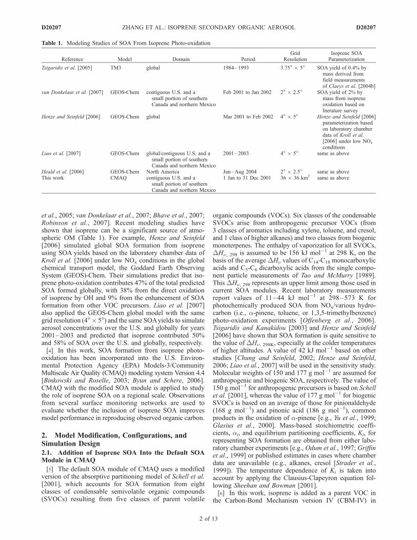
et al., 2005; van Donkelaar et al., 2007; Bhave et al., 2007;Robinson et al., 2007]. Recent modeling studies haveshown that isoprene can be a significant source of atmo-spheric OM (Table 1). For example, Henze and Seinfeld[2006] simulated global SOA formation from isopreneusing SOA yields based on the laboratory chamber data ofKroll et al. [2006] under low NOx conditions in the globalchemical transport model, the Goddard Earth ObservingSystem (GEOS)-Chem. Their simulations predict that iso-prene photo-oxidation contributes 47% of the total predictedSOA formed globally, with 38% from the direct oxidationof isoprene by OH and 9% from the enhancement of SOAformation from other VOC precursors. Liao et al. [2007]also applied the GEOS-Chem global model with the samegrid resolution (4�� 5�) and the same SOAyields to simulateaerosol concentrations over the U.S. and globally for years2001–2003 and predicted that isoprene contributed 50%and 58% of SOA over the U.S. and globally, respectively.[4] In this work, SOA formation from isoprene photo-

oxidation has been incorporated into the U.S. Environ-mental Protection Agency (EPA) Models-3/CommunityMultiscale Air Quality (CMAQ) modeling system Version 4.4[Binkowski and Roselle, 2003; Byun and Schere, 2006].CMAQ with the modified SOA module is applied to studythe role of isoprene SOA on a regional scale. Observationsfrom several surface monitoring networks are used toevaluate whether the inclusion of isoprene SOA improvesmodel performance in reproducing observed organic carbon.

2. Model Modification, Configurations, andSimulation Design

2.1. Addition of Isoprene SOA Into the Default SOAModule in CMAQ

[5] The default SOA module of CMAQ uses a modifiedversion of the absorptive partitioning model of Schell et al.[2001], which accounts for SOA formation from eightclasses of condensable semivolatile organic compounds(SVOCs) resulting from five classes of parent volatile

organic compounds (VOCs). Six classes of the condensableSVOCs arise from anthropogenic precursor VOCs (from3 classes of aromatics including xylene, toluene, and cresol,and 1 class of higher alkanes) and two classes from biogenicmonoterpenes. The enthalpy of vaporization for all SVOCs,DHn, 298 is assumed to be 156 kJ mol�1 at 298 K, on thebasis of the averageDHn values of C14-C18 monocarboxylicacids and C5-C6 dicarboxylic acids from the single compo-nent particle measurements of Tao and McMurry [1989].ThisDHn, 298 represents an upper limit among those used incurrent SOA modules. Recent laboratory measurementsreport values of 11–44 kJ mol�1 at 298–573 K forphotochemically produced SOA from NOx/various hydro-carbon (i.e., a-pinene, toluene, or 1,3,5-trimethylbenzene)photo-oxidation experiments [Offenberg et al., 2006].Tsigaridis and Kanakidou [2003] and Henze and Seinfeld[2006] have shown that SOA formation is quite sensitive tothe value of DHn, 298K, especially at the colder temperaturesof higher altitudes. A value of 42 kJ mol�1 based on otherstudies [Chung and Seinfeld, 2002; Henze and Seinfeld,2006; Liao et al., 2007] will be used in the sensitivity study.Molecular weights of 150 and 177 g mol�1 are assumed foranthropogenic and biogenic SOA, respectively. The value of150 g mol�1 for anthropogenic precursors is based on Schellet al. [2001], whereas the value of 177 g mol�1 for biogenicSVOCs is based on an average of those for pinionaldehyde(168 g mol�1) and pinonic acid (186 g mol�1), commonproducts in the oxidation of a-pinene [e.g., Yu et al., 1999;Glasius et al., 2000]. Mass-based stoichiometric coeffi-cients, ai, and equilibrium partitioning coefficients, Ki, forrepresenting SOA formation are obtained from either labo-ratory chamber experiments [e.g., Odum et al., 1997; Griffinet al., 1999] or published estimates in cases where chamberdata are unavailable (e.g., alkanes, cresol [Strader et al.,1999]). The temperature dependence of Ki is taken intoaccount by applying the Clausius-Clapeyron equation fol-lowing Sheehan and Bowman [2001].[6] In this work, isoprene is added as a parent VOC in

the Carbon-Bond Mechanism version IV (CBM-IV) in

Table 1. Modeling Studies of SOA From Isoprene Photo-oxidation

Reference Model Domain PeriodGrid

ResolutionIsoprene SOAParameterization

Tsigaridis et al. [2005] TM3 global 1984–1993 3.75� � 5� SOA yield of 0.4% bymass derived fromfield measurementsof Claeys et al. [2004b]

van Donkelaar et al. [2007] GEOS-Chem contiguous U.S. and asmall portion of southernCanada and northern Mexico

Feb 2001 to Jan 2002 2� � 2.5� SOA yield of 2% bymass from isopreneoxidation based onliterature survey

Henze and Seinfeld [2006] GEOS-Chem global Mar 2001 to Feb 2002 4� � 5� Henze and Seinfeld [2006]parameterization basedon laboratory chamberdata of Kroll et al.[2006] under low NOx

conditionsLiao et al. [2007] GEOS-Chem global/contiguous U.S. and a

small portion of southernCanada and northern Mexico

2001–2003 4� � 5� same as above

Heald et al. [2006] GEOS-Chem North America Jun–Aug 2004 2� � 2.5� same as aboveThis work CMAQ contiguous U.S. and a

small portion of southernCanada and northern Mexico

1 Jan to 31 Dec 2001 36 � 36 km2 same as above

D20207 ZHANG ET AL.: ISOPRENE SECONDARY ORGANIC AEROSOL

2 of 13

D20207

CMAQ to account for SOA precursors from isoprenephoto-oxidation in the revised SOA module. It is taken tobe oxidized by the hydroxyl radical (OH) to produce twoclasses of condensable SVOCs:

Isopreneþ OH ! a1G1 þ a2G2

where a1 and a2 are the stoichiometric coefficients forSVOC products G1 and G2, representing high and low SOAyield products, respectively. SOA yield parameters (i.e., ai

and Ki) from isoprene photo-oxidation can be derived fromlaboratory data reported by Kroll et al. [2006] at low andhigh NOx conditions ([NOx]< 1 ppb and [NOx] > 120 ppb,respectively). Kroll et al. [2006] observed an increase inSOA formation under low NOx conditions relative to highNOx conditions. Mixing ratios of NOx on a regional scaletend to lie in the range of 0.1–10 ppb; therefore thelaboratory chamber data at low NOx conditions areappropriate, and the parameterization of Henze and Seinfeld[2006] based on laboratory data of Kroll et al. [2006] isused in this work (Note that the crucial parameter is the[RO2]/[NO] ratio, not simply the NOx level). Table 2 showsthe SOA precursor classes and relevant parameters used inthe revised SOA formation mechanism in CMAQ.

2.2. Model Configurations and Simulation Design

[7] CMAQ baseline and sensitivity simulations are con-ducted at a horizontal grid spacing of 36 � 36 km2 and avertical resolution of 14 layers from the surface to 14.6 km(the first model layer is from 0 to 35 m) over a domaincovering the contiguous U.S. and a portion of southernCanada and northern Mexico. Meteorological fields aregenerated using the Pennsylvania State University/NationalCenter for Atmospheric Research Mesoscale ModelingSystem Generation 5 (MM5) Version 3.6.1 with four-dimensional data assimilation. Primary emissions of gaseousand aerosol species are based on the U.S. EPA’s NationalEmissions Inventories (NEI) 2001 with isoprene emissionsgenerated using the U.S. EPA’s Biogenic Emissions Inven-tory System (BEIS) version v. 3.12. Initial and boundaryconditions (ICONs and BCONs) are based on results from aglobal simulation using GEOS-Chem and the chemistry ofPark et al. [2004] at a 2� � 2.5� horizontal resolution. TheGEOS-Chem 2001 simulation uses a 3-month spin-upperiod (1 October to 31 December 2000) and is driven byassimilated meteorological observations from the GoddardEarth Observing System (GEOS) of the NASA Global

Modeling and Assimilation Office [Park et al., 2004]. TheCMAQ 2001 simulations use the boundary conditionsfrom GEOS-Chem every 3 h and a spin-up period of 10 d(22–31 December 2000).[8] Two baseline CMAQ simulations with the current

EPA default SOA module are conducted: a 1-a (i.e., year2001) simulation with DHn, 298 of 156 kJ mol�1 for allSVOCs (Base 1) and a 1-month (i.e., July 2001) simulationwith DHn, 298 of 42 kJ mol�1 for all SVOCs (Base 2) toprovide baseline results at two different values of DHn, 298.Since the same value of 156 kJ mol�1 DHn, 298 is used forall SVOCs, changing DHn, 298 will affect not only isopreneSOA but also SOA from other SVOCs, making it difficult toisolate the net sensitivity of isoprene SOA to the value ofDHn, 298. It is therefore necessary to conduct the two pairsof simulations in the presence and absence of isopreneSOA with the DHn, 298 value of 156 (Base 1 and Sen 1) or42 kJ mol�1 (Base 2 and Sen 3) and compare the relativecontribution of isoprene SOA to biogenic SOA at differentDHn, 298 values to isolate the sensitivity of isoprene SOAformation to the value of DHn, 298. Sensitivity simulationswith the revised SOA module are therefore conducted foryear 2001 with DHn, 298 of 156 kJ mol�1 for all SVOCs(Sen 1) and for July 2001 with DHn, 298 of 42 kJ mol�1 forall SVOCs (Sen 3) to intercompare results from Base 1 andBase 2, respectively. The 1-a simulation pair of Base 1 andSen 1 and 1-month simulation pair of Base 2 and Sen 3provide an assessment of the role of isoprene in SOAformation at two different values of DHn, 298 that arecurrently used 3-D models.[9] In addition to the volatility of SOA (as reflected in the

enthalpy of vaporization, DHn), parent hydrocarbon emis-sion is another influential parameter determining atmo-spheric SOA formation. Compared with BEIS v. 3.12 thatis used in the baseline simulations, BEIS v. 3.13 signifi-cantly lowers isoprene emissions for two reasons. First, theemission factor for spruce used in BEIS v3.13 is about afactor of 2 lower than that used in BEIS v. 3.12 [Schwede etal., 2005]. Second, the two BEIS versions use differentempirical coefficients in the adjustment factor for the effectsof photosynthetically active radiation (PAR) that largelyaffects isoprene emissions. The updated coefficients basedon the empirical equation of Guenther et al. [1999] in BEISv.3.13 lead to a decrease in the PAR adjustment factor that isused in BEIS v.3.12. As a result of the lower emission andPAR adjustment factors used in BEIS v. 3.13, isoprene

Table 2. SOA Precursor Classes and Relevant Parameters Used in the Revised CMAQ

Parent GaseousPrecursors

MolecularWeight, g mol�1

SOA PrecursorClasses

MolecularWeight, g mol�1

DHn, 298,a

kJ mol�1 aia Ki, 298,

a,b m3 mg�1

Higher alkanes 114 Alkane 150 156 0.0718 3.2227Xylene 106 Xylene_1, Xylene_2 150, 150 156, 156 0.038, 0.167 0.4619, 0.0154Cresol 108 Cresol 150 156 0.05 3.8300Toluene 92 Toluene_1, Toluene_2 150, 150 156, 156 0.071, 0.138 0.5829, 0.0209Terpenes 136 Terpenes_1, Terpenes_2 177, 177 156, 156 0.0864, 0.3857 1.1561, 0.0847Isoprenec (low NOx) 68 Isoprene_1, Isoprene_2 177, 177 156, 156 0.232, 0.0288 0.00459, 0.8628

aDHn, the enthalpy of vaporization of SOA; ai, stoichiometric coefficients; Ki, equilibrium partitioning coefficient.bKi, 298 is derived on the basis of laboratory chamber measurements of Kroll et al. [2006] under low NOx conditions at a reference temperature of 295 K

by applying the Clausius-Clapeyron equation following Sheehan and Bowman [2001].cIncorporated into the original CMAQ SOA module in this work. SOA yield parameters under low NOx conditions of Henze and Seinfeld [2006] are

used.


3 of 13

D20207

emissions estimated from BEIS v. 3.13 are up to 60% lowerthan those from BEIS v. 3.12, with reductions over largeareas in southern Canada (30–60%), northern Mexico (10–50%), eastern U.S. (20–40%), and western U.S. (10–40%).To study the sensitivity of model predictions to isopreneemissions, a 1-month (i.e., July 2001) simulation with therevised SOA module, DHn, 298 of 156 kJ mol�1 for allSVOCs, and BEIS v. 3.13 isoprene emissions (Sen 2) is alsoconducted and compared with Sen 1. Table 3 summarizes theconfigurations of the baseline and sensitivity simulations.[10] Results from the two 1-a CMAQ simulations (Base 1

and Sen 1) are compared to assess the contribution ofisoprene to SOA formation, its seasonal variations andspatial distributions on a regional scale, its impact on thenet export of SOA from the planetary boundary layer (PBL)and on the formation of anthropogenic SOA. Predictedconcentrations for key species such as O3 and particulatematter and organic carbon with an aerodynamic diameterequal or less than 2.5 mm (PM2.5 and OC2.5) are evaluatedagainst available observations. Process analysis using theIntegrated Process Rates (IPRs) and the Integrated ReactionRates (IRRs) methods embedded in CMAQ is also con-ducted to identify the atmospheric processes controllingSOA formation as well as key reactions for its gaseousprecursors. The IPRs quantify the contributions of physical(e.g., advection, diffusion, emission, chemistry, dry and wetdeposition) and chemical processes (e.g., gas and aqueousphase chemistry) to changes in species concentrations. TheIRRs provide the individual gas phase reaction rates, thuspermitting a detailed study of chemical transformation ofthe species of interest.

3. Analyses of 1-a Simulations in the Absence andPresence of Isoprene SOA

[11] Mixing ratios of isoprene and other SOA precursorsare not conventionally measured in the U.S. EPA surface

monitoring networks; measurements of other relevant spe-cies such as O3, and PM2.5 and total column abundance ofseveral species/parameters such as CO, NOx, and aerosoloptical depth (AOD), are, however, available on a regionalscale from several surface networks and satellite instru-ments. Results from CMAQ 2001 baseline and sensitivitysimulations (Base 1 and Sen 1) are therefore evaluated usingavailable surface and satellite observations for O3, NOx,CO, PM2.5, PM2.5 composition, and AOD. Surface moni-toring networks include the Clean Air Status and TrendsNetwork (CASTNet) (http://www.epa.gov/castnet/), theAerometric Information Retrieval System (AIRS)-AirQuality System (AQS) (http://www.epa.gov/air/data/index.html), the Speciation Trends Network (STN), theInteragency Monitoring of Protected Visual Environments(IMPROVE) (http://vista.cira.colostate.edu/improve/), andthe Southeastern Aerosol Research and Characterizationstudy (SEARCH) (http://www.atmospheric-research.com/studies/SEARCH/). Satellite data include the TroposphericO3 Residual (TOR) derived from the Total Ozone MappingSpectrometer (TOMS) and the Solar Backscatter Ultraviolet(SBUV), the tropospheric CO columns derived from theMeasurements Of Pollution In The Troposphere (MOPITT)instrument, the tropospheric NO2 columns derived using theDifferential Optical Absorption method from the GlobalOzone Monitoring Experiment (GOME) instrument, and thetotal AOD estimated from the Moderate Resolution ImagingSpectroradiometer (MODIS). Overall CMAQ model perfor-mance is consistent with that of current 3-D air qualitymodels [Zhang et al., 2005, 2006c]. As an example, Tables 4aand 4b show performance statistics for CMAQ predictionsof maximum 8-h average O3 mixing ratios at surface andtotal tropospheric NO2 column abundance from Base 1 (theresults from Sen 1 are very similar, thus not shown). Thenormalized mean biases (NMBs) for maximum 8-h averageO3 mixing ratios are small (�10.6% to �2% for CASTNetsites and �1.5% to 3% for AIRS-AQS sites) and those for

Table 3. Model Configurations for Baseline and Sensitivity Simulations

Simulation Period Isoprene Emission DHn, 298K, kJ mol�1 SOA Module Isoprene SOA Yields Process Analysis

Base 1 1 Jan to 31 Dec 2001 BEIS v. 3.12 156 default CMAQ N/A 1 Jan to 31 Dec 2001Base 2 1–31 Jul 2001 BEIS v. 3.12 42 default CMAQ N/A Jan, Apr, Jul, and Oct 2001Sen 1 1 Jan to 31 Dec 2001 BEIS v. 3.12 156 revised CMAQ low NOx conditions noneSen 2 1–31 Jul 2001 BEIS v. 3.13 156 revised CMAQ low NOx conditions noneSen 3 1–31 Jul 2001 BEIS v. 3.12 42 revised CMAQ low NOx conditions none

Table 4a. Performance Statistics of CMAQ 2001 Baseline Simulation Without Isoprene SOA: Maximum 8-h Average Surface O3

Mixing Ratiosa

Variables

Winter Spring Summer Fall

CASTNet AIRS-AQS CASTNet AIRS-AQS CASTNet AIRS-AQS CASTNet AIRS-AQS

MeanObs 32.31 29.31 49.32 49.71 52.25 54.26 40.94 41.74MeanMod 28.87 29.59 48.34 51.18 51.05 55.40 38.46 41.11Number 6,186 45,782 6,433 83,759 6,569 101,515 6,669 78,712Correlation 0.69 0.58 0.71 0.68 0.63 0.70 0.68 0.69NMB, % �10.6 1.0 �2.0 3.0 �2.3 2.1 �6.1 �1.5NME, % 21.7 25.4 14.6 16.3 17.3 18.3 18.9 19.6

aUnit is ppb.


4 of 13

D20207

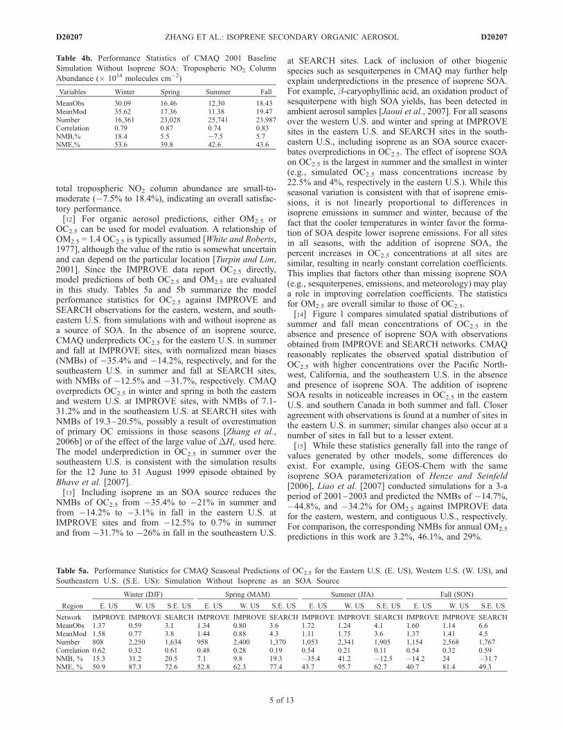
total tropospheric NO2 column abundance are small-to-moderate (�7.5% to 18.4%), indicating an overall satisfac-tory performance.[12] For organic aerosol predictions, either OM2.5 or

OC2.5 can be used for model evaluation. A relationship ofOM2.5 = 1.4 OC2.5 is typically assumed [White and Roberts,1977], although the value of the ratio is somewhat uncertainand can depend on the particular location [Turpin and Lim,2001]. Since the IMPROVE data report OC2.5 directly,model predictions of both OC2.5 and OM2.5 are evaluatedin this study. Tables 5a and 5b summarize the modelperformance statistics for OC2.5 against IMPROVE andSEARCH observations for the eastern, western, and south-eastern U.S. from simulations with and without isoprene asa source of SOA. In the absence of an isoprene source,CMAQ underpredicts OC2.5 for the eastern U.S. in summerand fall at IMPROVE sites, with normalized mean biases(NMBs) of �35.4% and �14.2%, respectively, and for thesoutheastern U.S. in summer and fall at SEARCH sites,with NMBs of �12.5% and �31.7%, respectively. CMAQoverpredicts OC2.5 in winter and spring in both the easternand western U.S. at IMPROVE sites, with NMBs of 7.1-31.2% and in the southeastern U.S. at SEARCH sites withNMBs of 19.3–20.5%, possibly a result of overestimationof primary OC emissions in those seasons [Zhang et al.,2006b] or of the effect of the large value of DHn used here.The model underprediction in OC2.5 in summer over thesoutheastern U.S. is consistent with the simulation resultsfor the 12 June to 31 August 1999 episode obtained byBhave et al. [2007].[13] Including isoprene as an SOA source reduces the

NMBs of OC2.5 from �35.4% to �21% in summer andfrom �14.2% to �3.1% in fall in the eastern U.S. atIMPROVE sites and from �12.5% to 0.7% in summerand from �31.7% to �26% in fall in the southeastern U.S.

at SEARCH sites. Lack of inclusion of other biogenicspecies such as sesquiterpenes in CMAQ may further helpexplain underpredictions in the presence of isoprene SOA.For example, b-caryophyllinic acid, an oxidation product ofsesquiterpene with high SOA yields, has been detected inambient aerosol samples [Jaoui et al., 2007]. For all seasonsover the western U.S. and winter and spring at IMPROVEsites in the eastern U.S. and SEARCH sites in the south-eastern U.S., including isoprene as an SOA source exacer-bates overpredictions in OC2.5. The effect of isoprene SOAon OC2.5 is the largest in summer and the smallest in winter(e.g., simulated OC2.5 mass concentrations increase by22.5% and 4%, respectively in the eastern U.S.). While thisseasonal variation is consistent with that of isoprene emis-sions, it is not linearly proportional to differences inisoprene emissions in summer and winter, because of thefact that the cooler temperatures in winter favor the forma-tion of SOA despite lower isoprene emissions. For all sitesin all seasons, with the addition of isoprene SOA, thepercent increases in OC2.5 concentrations at all sites aresimilar, resulting in nearly constant correlation coefficients.This implies that factors other than missing isoprene SOA(e.g., sesquiterpenes, emissions, and meteorology) may playa role in improving correlation coefficients. The statisticsfor OM2.5 are overall similar to those of OC2.5.[14] Figure 1 compares simulated spatial distributions of

summer and fall mean concentrations of OC2.5 in theabsence and presence of isoprene SOA with observationsobtained from IMPROVE and SEARCH networks. CMAQreasonably replicates the observed spatial distribution ofOC2.5 with higher concentrations over the Pacific North-west, California, and the southeastern U.S. in the absenceand presence of isoprene SOA. The addition of isopreneSOA results in noticeable increases in OC2.5 in the easternU.S. and southern Canada in both summer and fall. Closeragreement with observations is found at a number of sites inthe eastern U.S. in summer; similar changes also occur at anumber of sites in fall but to a lesser extent.[15] While these statistics generally fall into the range of

values generated by other models, some differences doexist. For example, using GEOS-Chem with the sameisoprene SOA parameterization of Henze and Seinfeld[2006], Liao et al. [2007] conducted simulations for a 3-aperiod of 2001–2003 and predicted the NMBs of �14.7%,�44.8%, and �34.2% for OM2.5 against IMPROVE datafor the eastern, western, and contiguous U.S., respectively.For comparison, the corresponding NMBs for annual OM2.5

predictions in this work are 3.2%, 46.1%, and 29%.

Table 4b. Performance Statistics of CMAQ 2001 Baseline

Simulation Without Isoprene SOA: Tropospheric NO2 Column

Abundance (� 1014 molecules cm�2)

Variables Winter Spring Summer Fall

MeanObs 30.09 16.46 12.30 18.43MeanMod 35.62 17.36 11.38 19.47Number 16,361 23,028 25,741 23,987Correlation 0.79 0.87 0.74 0.83NMB,% 18.4 5.5 �7.5 5.7NME,% 53.6 39.8 42.6 43.6

Table 5a. Performance Statistics for CMAQ Seasonal Predictions of OC2.5 for the Eastern U.S. (E. US), Western U.S. (W. US), and

Southeastern U.S. (S.E. US): Simulation Without Isoprene as an SOA Source

Region

Winter (DJF) Spring (MAM) Summer (JJA) Fall (SON)

E. US W. US S.E. US E. US W. US S.E. US E. US W. US S.E. US E. US W. US S.E. US

Network IMPROVE IMPROVE SEARCH IMPROVE IMPROVE SEARCH IMPROVE IMPROVE SEARCH IMPROVE IMPROVE SEARCHMeanObs 1.37 0.59 3.1 1.34 0.80 3.6 1.72 1.24 4.1 1.60 1.14 6.6MeanMod 1.58 0.77 3.8 1.44 0.88 4.3 1.11 1.75 3.6 1.37 1.41 4.5Number 808 2,250 1,634 958 2,400 1,370 1,053 2,341 1,905 1,154 2,568 1,767Correlation 0.62 0.32 0.61 0.48 0.28 0.19 0.54 0.21 0.11 0.54 0.32 0.59NMB, % 15.3 31.2 20.5 7.1 9.8 19.3 �35.4 41.2 �12.5 �14.2 24 �31.7NME, % 50.9 87.3 72.6 52.8 62.3 77.4 43.7 95.7 62.7 40.7 81.4 49.3


5 of 13

D20207

[16] While both GEOS-Chem and modified CMAQ usethe same equilibrium partitioning equations and experimen-tally determined partitioning coefficients and SOA yields,some differences exist. First, the condensable SVOCs ineach model differ. Modified CMAQ used in this work treatssix parent precursors: four anthropogenic (i.e., higher alka-nes, xylene, toluence, and cresol) and two biogenic (i.e.,isoprene and terpene with an arithmetic mean of partitioningcoefficients and SOA yield coefficients of a-pinene, b-pinene, sabinene, D3-carene, and limonene). ModifiedGEOS-Chem used by Liao et al. [2007] treats six classesof biogenic parent compounds including isoprene, class Iterpene (i.e., a-pinene, b-pinene, sabinene, D3-carene, andlimonene), class II terpene (i.e., limonene), class III terpene

(a-terpinene, g-terpinene, and terpinolene), class IV terpene(i.e., myrcene, terpenoid alcohols, ocimene), and class V(i.e., sesquiterpenes). Second, the SOA modules in the twomodels, as implemented, use different values of DHn, 298,42 kJ mol�1 for GEOS-Chem and 156 kJ mol�1 for CMAQ.Given the high sensitivity of SOA formation to DHn, 298

[Tsigaridis and Kanakidou, 2003; Henze and Seinfeld,2006], significantly higher SOA concentrations result at alarger value of DHn, 298. Third, gas phase chemical mech-anisms in the two models differ, resulting in different ratesand levels of conversions of SOA precursors. Fourth, differ-ences exist in model inputs such as meteorological fieldsand emissions. The large underprediction in OM2.5 byGEOS-Chem for the western U.S. has been attributed to

Table 5b. Performance Statistics for CMAQ Seasonal Predictions of OC2.5 for the Eastern U.S. (E. US), Western U.S. (W. US), and

Southeastern U.S. (S.E. US): Simulation With Isoprene as an SOA Source

Region

Winter (DJF) Spring (MAM) Summer (JJA) Fall (SON)

E. US W. US S.E. US E. US W. US S.E. US E. US W. US S.E. US E. US W. US S.E. US

Network IMPROVE IMPROVE SEARCH IMPROVE IMPROVE SEARCH IMPROVE IMPROVE SEARCH IMPROVE IMPROVE SEARCHMeanObs 1.37 0.59 3.1 1.34 0.80 3.6 1.72 1.24 4.1 1.60 1.14 6.6MeanMod 1.65 0.84 3.8 1.57 0.97 4.5 1.36 1.92 4.1 1.55 1.58 4.9Number 808 2,250 1,634 958 2,400 1,370 1,053 2,341 1,905 1,154 2,568 1,767Correlation 0.62 0.33 0.61 0.50 0.29 0.19 0.56 0.22 0.12 0.53 0.33 0.59NMB, % 20.6 42.7 21.9 17.1 21.6 26.1 �21.0 55.2 0.7 �3.1 38.8 �26NME, % 53.0 93.5 72.9 53.9 67.3 81.8 38.4 102.4 65.8 43.1 89.7 47.8

Figure 1. Overlay of simulated and observed spatial distributions of 2001 summer and fall meanconcentrations of OC2.5 in the (a) absence and (b) presence of isoprene SOA.


6 of 13

D20207

unaccounted primary OM emissions from some sourcessuch as large wildfires over the U.S. in year 2002 [Liao etal., 2007]. By contrast, primary OM emissions used inCMAQ simulations may be overestimated. The differencesin simulated SOA, model treatments, and model inputs inthe two models demonstrate the challenges in modelingSOA.[17] Figure 2 shows predicted annual mean biogenic SOA

concentrations from isoprene photo-oxidation at the surface,in the PBL (0–2.85 km), in the free troposphere (FT)(2.85–9 km), and in the upper troposphere (UT) (9–14.6 km). Isoprene photo-oxidation contributes to annualmean biogenic SOA concentrations by up to 0.54, 3.8, 0.44,and 0.04 mg m�3 at the surface, in the PBL, the FT, and theUT, respectively, in the modeling domain. Surface-level(i.e., 0–35 m) biogenic SOA concentrations resulting fromdirect isoprene emissions over the western U.S. are rela-tively low (mostly < 0.2 mg m�3), reaching 0.8–2.8 mg m�3

in the PBL over most of western states in the U.S. andnorthern Mexico. Elevated biogenic SOA concentrations arepredicted to occur in the FT over northern Mexico, thesoutheastern U.S., and some areas in the states of Utah,Colorado, Arizona, and New Mexico and in the UT over thesoutheastern U.S., where mesoscale convection systemsfrequently develop, particularly in summer and spring[Zajac and Rutledge, 2001; Orville and Huffines, 2001].

While high temperatures at or near the surface do not favorthe condensation of semivolatile isoprene oxidation prod-ucts, strong convective updrafts transport isoprene andresultant SVOCs to higher altitudes where SOA can thenform; convective mixing and subtropical jet streams resultin a more uniform spatial distribution in the FT and the UT.[18] Edney et al. [2006] conducted field measurements

over the period of 12 January to 29 December 2003 in thesoutheastern U.S. and estimated the highest isoprene SOAconcentrations of �1 mgC m�3 (�1.2 mg m�3) in July–August using an organic tracer method. This amount isgenerally consistent with the CMAQ simulated value of0.5–0.9 mg m�3 in the southeastern U.S. in July–August(figure not shown). Isoprene SOA is predicted to lead to anincrease of total biogenic SOA, total OM (OM = primaryorganic aerosols (POA) + anthropogenic SOA + biogenicSOA), and total PM2.5 by up to 117%, 65%, and 25%,respectively, at the surface; 110%, 56%, and 22%, respec-tively, in the PBL; 147%, 90%, 33%, respectively, in the FT;and 237%, 79%, and 19%, respectively in the UT overNorth America.[19] Figure 3 shows the predicted percent contributions of

isoprene photo-oxidation to anthropogenic SOA, biogenicSOA, and total SOA as a function of altitude in terms ofannual mean values in the entire modeling domain. Isoprenephoto-oxidation leads to an increase in domainwide biogenic

Figure 2. Predicted annual mean biogenic SOA concentrations from isoprene photo-oxidation (a) at thesurface (0–35m), (b) in the planetary boundary layer (0–2.85 km), (c) in the free troposphere (2.85–9 km),and (d) in the upper troposphere (9–14.6 km).


7 of 13

D20207

SOA and total SOA concentrations by 0.0165–0.15 mg m�3

(38–131%) and 0.0165–0.154 mg m�3 (35–105%), respec-tively, with the larger changes for biogenic SOA occurringin the eastern domain. The domain average percent contri-bution of isoprene SOA from the surface to the UT exhibitsa strong seasonal variation with a maximum in summer anda minimum in winter. With isoprene as a source of SOA,anthropogenic SOA increases by 1–10%, as shown inFigure 3; this is caused by perturbations in the gas-aerosolequilibrium system. Given the total concentration of SVOCspecies i, gas/aerosol partitioning equilibrium is governedby the partitioning coefficient, Ki, and total absorbingorganic mass, M0. M0 is calculated as the sum of concen-trations of primary and secondary OM. Isoprene SOAincreases M0, which shifts the gas-aerosol equilibriumtoward the aerosol phase, thus increasing aerosol phaseconcentration of SVOCs.[20] The Integrated Process Rates are calculated to quan-

tify the relative contributions of major atmospheric process-es to total biogenic SOA concentrations. Figure 4 shows theannual mean process contribution for year 2001 to totaldomainwide biogenic SOA concentrations in the PBL inthe presence and absence of isoprene SOA. Aerosolprocesses lead to biogenic SOA at an annual average rateof 26.64 Gg d�1 (i.e., 9.72 Tg a�1) from all sources other

than isoprene within the PBL. This annual mean productionrate increases by 54% from 26.64 to 41.13 Gg d�1 (i.e.,from 9.72 to 15 Tg a�1) when isoprene SOA is included. Itis important to note that those annual average rates may

Figure 3. Annual mean (a) absolute and (b) percent increases over the modeling domain as a functionof altitude in anthropogenic SOA (ASOA), biogenic SOA (BSOA), and total SOA (TSOA) due to theinclusion of isoprene as a source of SOA.

Figure 4. Annual mean domain average process contribu-tions in 2001 to total biogenic SOA concentrations in thePBL with and without isoprene SOA.


8 of 13

D20207

represent upper limits, because of the large value of DHn,

298 used. Cloud processes and dry deposition removebiogenic SOA from the atmosphere, and diffusion andadvection help vent it out of the PBL to the FT and/oroutside of the modeling domain. The total net annual exportof biogenic SOA from the PBL in the modeling domain tothe FT is 20.68 Gg d�1 (i.e., 7.55 Tg a�1) without isopreneSOA and 32.49 Gg d�1 (i.e., 11.86 Tg a�1) with isopreneSOA (increased by a factor of 1.6).

4. Sensitivity to Isoprene Emissions and theEnthalpy of Vaporization of SVOCs

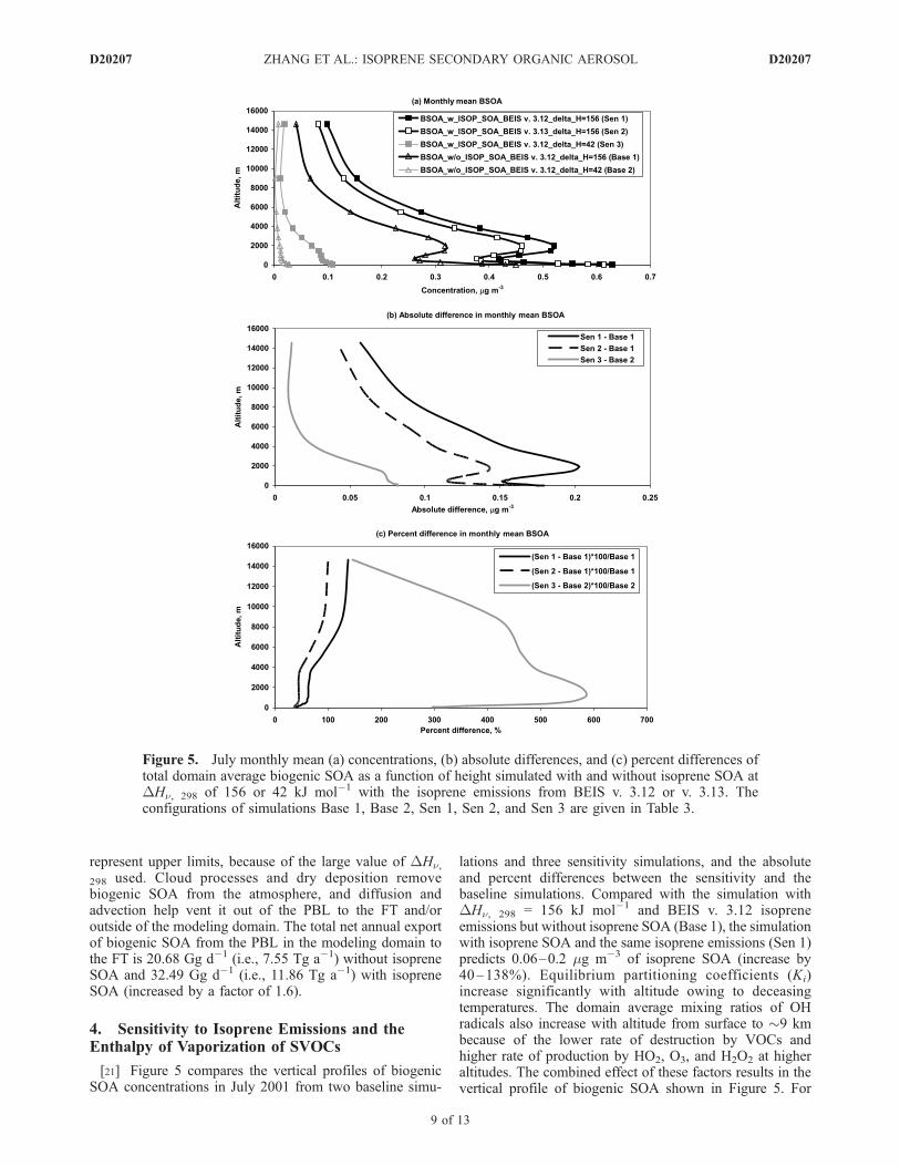
[21] Figure 5 compares the vertical profiles of biogenicSOA concentrations in July 2001 from two baseline simu-

lations and three sensitivity simulations, and the absoluteand percent differences between the sensitivity and thebaseline simulations. Compared with the simulation withDHn, 298 = 156 kJ mol�1 and BEIS v. 3.12 isopreneemissions but without isoprene SOA (Base 1), the simulationwith isoprene SOA and the same isoprene emissions (Sen 1)predicts 0.06–0.2 mg m�3 of isoprene SOA (increase by40–138%). Equilibrium partitioning coefficients (Ki)increase significantly with altitude owing to deceasingtemperatures. The domain average mixing ratios of OHradicals also increase with altitude from surface to �9 kmbecause of the lower rate of destruction by VOCs andhigher rate of production by HO2, O3, and H2O2 at higheraltitudes. The combined effect of these factors results in thevertical profile of biogenic SOA shown in Figure 5. For

Figure 5. July monthly mean (a) concentrations, (b) absolute differences, and (c) percent differences oftotal domain average biogenic SOA as a function of height simulated with and without isoprene SOA atDHn, 298 of 156 or 42 kJ mol�1 with the isoprene emissions from BEIS v. 3.12 or v. 3.13. Theconfigurations of simulations Base 1, Base 2, Sen 1, Sen 2, and Sen 3 are given in Table 3.


9 of 13

D20207

example, the decrease in the mixing ratio of isoprene (andthus its SVOC products) may predominate below 0.65 kmand above 2 km, causing biogenic SOA concentrations todecrease with increasing height, whereas between 0.65 and2 km, the effect due to the increase in Ki may dominate.[22] Compared with Base 1 and Sen 1, the use of BEIS v.

3.13 isoprene emissions in Sen 2 produces a decline in thesurface level monthly mean mixing ratios of isoprene by20–60% in the western U.S., 40–60% in the eastern U.S.,40–70% in northern Mexico, and 50–70% in southernCanada. Compared with Sen 1, lower isoprene emissionsin Sen 2 cause a decrease in the domain average biogenicSOA concentrations by 2.6%, 8.1%, 14.2%, and 16% at thesurface, in the PBL, FT, and UT, respectively. The relativelysmall percent decreases at the surface and below 2 km aredue to changes in the chemical system resulting fromreduced isoprene emissions (see explanation below). Above2 km, the chemical perturbation is smaller with a nearlyconstant decrease in biogenic SOA concentrations fromSen 1, but the relative impact of reduced isoprene emissionson biogenic SOA formation becomes more pronounced(because of lower Base 1 SOA concentrations) at higheraltitudes. The percent decreases in biogenic SOA through-out the atmosphere are lower than those in isoprene emis-sions, particularly at the surface. This is a result of changesin concentrations of related species such as OH and SVOCsformed from photo-oxidation of isoprene and terpenesbecause of lower isoprene emission and the nonlinearityin biogenic SOA formation that depends on mixing ratios ofprecursors (e.g., SVOCs formed via oxidation of terpenesand isoprene) and oxidants (e.g., OH). Lower isopreneemissions result in lower formaldehyde (by 10.9%,10.4%, 4.5%, and 6.4% domain average at surface, in thePBL, FT, and UT, respectively), lower carbon monoxide (by1.1%, 1.2%, 0.9%, and 0.7% domain average at surface, inthe PBL, FT, and UT, respectively), and higher OH mixingratios (by 7.8%, 6.6%, 3.1%, and 2.7% domain average atsurface, in the PBL, FT, and UT, respectively). The magni-tude of those changes in regions with large isopreneemissions can be much higher. For example, the mixingratios of OH increase by up to 30% in the western U.S., 10–50% in the eastern U.S., 30–60% in southern Canada, andup to 70% in northern Mexico. Higher OH levels lead togreater oxidation of terpenes; consequently, the mixingratios of terpenes are lower by 11.5%, 17.7%, 20.4%, and21.5% domain average at surface, in the PBL, FT, and UT,respectively. Reactions of terpenes dominate biogenic SOAformation below �5 km, contributing to �56–68% ofbiogenic SOA with BEIS v. 3.12 isoprene emissions and�67–78% of biogenic SOA with BEIS v. 3.13 isopreneemissions. As a result of a reduced fraction of isoprene SOAin biogenic SOA in Sen 2, the effect of lower isopreneemissions on SOA formation is smaller at and near thesurface.[23] The enthalpy of vaporization, DHn, 298, affects SOA

formation via Ki. For example, when temperature decreasesfrom 294.4 K to 225.7 K (corresponding to the domainaverage temperatures at surface and 14.6 km, respectively),Ki increases from 9.9 � 10�3 to 2 � 106 m3 mg�1 withDHn, 298 = 156 kJ mol�1 and from 8.9� 10�3 to 1.3 m3 mg�1

with DHn, 298 = 42 kJ mol�1. The net differences inbiogenic SOA between the two simulations with DHn, 298

of 42 kJ mol�1 (i.e., Sen 3-Base 2) are compared withthose between the two simulations with DHn, 298 of 156kJ mol�1 (i.e., Sen 1-Base 1) for July 2001, as shown inFigures 5b and 5c. For simulations with DHn, 298 of 42 kJmol�1 for all SVOC species (Base 2 and Sen 3), the totaldomain average biogenic SOA concentrations increase by0.01–0.08 mg m�3 (146–586%) in the presence of isopreneSOA as compared with 0.06–0.2 mg m�3 at 156 kJ mol�1

(Base 1 and Sen 1). The values of DHn affect the extrap-olation of Ki values from their experimentally determinedtemperature to a different temperature. The values of DHnfor nonisoprene SVOCs (e.g., terpenes) have typically beenmeasured at higher temperatures than for isoprene SVOCs(e.g., 310 K versus 295 K). Therefore the percent increasesin SOA due to isoprene SOA are much larger with a lowerDHn value because of much smaller terpene SOA concen-trations (decreased by factors of 12–24 when changingDHn from 150 to 42 kJ mol�1) and higher mass fractionsof isoprene SOA in total biogenic SOA (59–85% at DHn= 42 kJ mol�1 versus 29–58% at DHn = 150 kJ mol�1).At higher altitudes, the effects of DHn on the Ki values ofboth terpene and isoprene SVOCs eventually becomeequal, and the changes in mass fractions of terpene SOAwith DHn = 42 and 156 KJ mol�1 are smaller. Conse-quently, the differences in the percent increases of totalbiogenic SOA owing to isoprene SOA obtained with DHn= 42 and 156 KJ mol�1 become smaller with increasingaltitudes.[24] Biogenic SOA concentrations decrease substantially

when theDHn, 298 value is reduced from 156 to 42 kJ mol�1

for both simulation pairs with and without isoprene SOA.First, the Ki values decrease substantially (e.g., by a factorof 8 at 298 K) when the DHn value is reduced from 156 to42 kJ mol�1, causing lower SOA formation. Second, SOAyields are highly sensitive to the total absorbing organicmass, M0, especially at low M0 levels. For example, whenthe DHn value is reduced from 156 to 42 kJ mol�1, theSOA yield from monoterpenes can decrease by a factor of3–4 (e.g., from 30% to 7%) at relatively high M0 values(e.g.,M0 = 5 mg m�3 at 293 K) but by a factor of 10 or moreat low M0 values (e.g., from 46% to 4.6% at M0 = 1 mg m�3

and from 44.3% to 2.7% at M0 = 0.5 mg m�3 at 273 K)(P. Bhave, personal communication, 2007). Total CMAQsimulated OM (primary + secondary) concentrations arewell below 1–2 mg m�3 in summer 2001; therefore the totalbiogenic SOA concentrations decrease substantially whenreducingDHn from 156 to 42 kJ mol�1. Although simulatedOC2.5 concentrations using a value of DHn = 156 kJ mol�1

are more consistent with observations, it is difficult toconclude that this parameter is the sole important factorowing to uncertainties in ambient observations and otheraspects of the model. If, indeed, a value of DHn =42 kJ mol�1 is more consistent with the observed volatilityof SOA, the large discrepancy between predicted andobserved SOA levels at DHn = 42 kJ mol�1 points to amajor deficiency in predicted SOA mass.

5. Conclusions

[25] Simulation of atmospheric SOA represents the mostchallenging aspect of aerosol modeling, as accurate repre-sentations of emissions of organic precursors and gas phase


10 of 13

D20207

chemistry are needed for generation of semivolatile products,gas-aerosol partitioning of the semivolatile products, andremoval of the particles from the atmosphere. SOA oftencontributes one half or more of the total ambient OM, sosuch a simulation is an important component of aerosolmodels. The U.S. EPA CMAQ atmospheric model containsa treatment of SOA formation from biogenic and anthropo-genic precursors. In this work we report the addition ofisoprene as an SOA precursor to CMAQ version 4.4. In theabsence of isoprene, CMAQ simulations underpredict levelsof organic particulate matter over the eastern U.S. (this workand Bhave et al. [2007]); with the addition of isoprene,predicted levels increase appreciably, but overall organicaerosol is still underpredicted over large areas of the easternU.S., even if the upper limit value of the enthalpy ofvaporization of SVOCs is assumed. Isoprene SOA forma-tion is highly sensitive to isoprene emissions and theenthalpy of vaporization of SVOCs used in the simulations.When the enthalpy of vaporization is reduced from 156 to42 kJ mol�1, simulated biogenic SOA concentrationdecreases substantially because of large decreases in theequilibrium partitioning coefficient and the SOA yield.[26] Several possible explanations exist for the prevalent

underprediction of total organic aerosol, including thefollowing: (1) An important class or classes of precursororganics is currently not accounted for, including sesqui-terpenes, oligomers with high molecular weight and lowvolatility that are generated from accretion reactions, andmolecules that are generally classified as primary particulateemissions; (2) the SOA yields of one or more of theprecursors are understated; and/or (3) emissions of impor-tant precursor organics are underestimated. The predomi-nant class of SOA-forming species is biogenics, and theaddition of isoprene to that class represents a major contri-bution. There is strong evidence from recent laboratorychamber studies, in addition, that under typical ambientlow NOx conditions both biogenic and anthropogenic SOAyields are larger than those determined in past laboratorychamber experiments in which NOx levels have generallybeen higher than those in the atmosphere. Continuedattention to these issues will be needed in order to resolvediscrepancies between predictions and observations oforganic aerosol levels.

[27] Acknowledgments. The work at NCSU was supported byNASA Award NNG04GJ90G, NSF Career Award Atm-0348819, and theMemorandum of Understanding between the U.S. Environmental Protec-tion Agency (EPA) and the U.S. Department of Commerce’s NationalOceanic and Atmospheric Administration (NOAA) and under agreementDW13921548. The work at Caltech was supported by the Electric PowerResearch Institute. Thanks are due to Warren Peters, the U.S. EPA/OAQPS,and George Pouliot, Ken Schere, and Tom Pierce, the U.S. NOAA/EPA, forproviding meteorological fields, emission inventories, initial and boundaryconditions for the 2001 simulations and helpful discussions on BEIS v3.12and v3.13; to Krish Vijayaraghavan, AER, Inc., for conducting baselineCMAQ simulation with the default SOA module; to Eric Edgerton and RickSaylor, ARA, Inc., for providing the SEARCH OC measurement data; toSteve Howard and Alice Gilliland, the U.S. NOAA/EPA, for providingthe Fortran code for extracting data from CMAQ and the CASTNet,IMPROVE, and AIRS-AQS observational databases; and to Shaocai Yu,the U.S. NOAA/EPA, for providing the Fortran code for statistical calcu-lations. Thanks are also due to Prakash Bhave, the U.S. NOAA/EPA, forcalculating SOA yields from monoterpenes at different values of DHn, 298,absorbing organic mass, and temperatures as well as insightful diagnosticanalyses and discussions for low SOA formation at low values of DHn, 298from CMAQ, and to Jesse Kroll, Aerodyne Research, Inc., and Edward

Edney, the U.S. EPA, for helpful discussions on SOA formation mechanismfrom isoprene.

ReferencesAtkinson, R. (1994), Gas-phase tropospheric chemistry of organic com-pounds, J. Phys. Chem. Ref. Data Monogr., 2, 1–216.

Bhave, P. V., G. A. Pouliot, and M. Zheng (2007), Diagnostic model eva-luation for carbonaceous PM2.5 using organic markers measured in thesoutheastern U. S., Environ. Sci. Technol., 41(5), 1577–1583.

Binkowski, F. S., and S. J. Roselle (2003), Models-3 Community Multi-scale Air Quality (CMAQ) model aerosol component: 1. Model descrip-tion, J. Geophys. Res., 108(D6), 4183, doi:10.1029/2001JD001409.

Boge, O., Y. Miao, A. Plewka, and H. Herrmann (2006), Formation ofsecondary organic particle phase compounds from isoprene gas-phaseoxidation products: An aerosol chamber and field study, Atmos. Environ.,40, 2501–2509.

Byun, D., and K. L. Schere (2006), Review of the governing equations,computational algorithms, and other components of the Models-3 Com-munity Multiscale Air Quality (CMAQ) modeling system, Appl. Mech.Rev., 59, 51–77.

Chameides, W. L., R. W. Lindsay, J. Richardson, and C. S. Kiang (1988),The role of biogenic hydrocarbons in urban photochemical smog-Atlantaas a case study, Science, 241(4872), 1473–1475.

Chung, S. H., and J. H. Seinfeld (2002), Global distribution and climateforcing of carbonaceous aerosols, J. Geophys. Res., 107(D19), 4407,doi:10.1029/2001JD001397.

Claeys, M., et al. (2004a), Formation of secondary organic aerosols throughphotooxidation of isoprene, Science, 303, 1173–1176.

Claeys, M.,W.Wang, A. C. Ion, I. Kourtchev, A. Gelencser, andW.Maenhaut(2004b), Formation of secondary organic aerosols from isoprene and gas-phase oxidation products through reaction with hydrogen peroxide,Atmos. Environ., 38, 4093–4098.

Clements, A. L., and J. H. Seinfeld (2007), Detection and quantification of2-methyltetrols in ambient aerosol in the southeastern United States,Atmos. Environ., 41, 1825–1830.

Czoschke, N. M., M. Jang, and R. M. Kamens (2003), Effect of acidic seedon biogenic secondary organic aerosol growth, Atmos. Environ., 37,4287–4299.

Edney, E. O., T. E. Kleindiensta, M. Jaouib, M. Lewandowskia, J. H.Offenberga, W. Wang, and M. Claeys (2005), Formation of 2-methyltetrols and 2-methylglyceric acid in secondary organic aerosol from la-boratory irradiated isoprene/NOx/SO2/air mixtures and their detection inambient PM2.5 samples collected in the eastern United States, Atmos.Environ., 39, 5281–5289.

Edney, E. O., M. Jaoui, M. Lewandowski, J. H. Offenberg, and T. E.Kleindienst (2006), Contribution of SOA and biomass burning to ambientPM2.5 organic carbon concentrations in Research Triangle Park, N. C.,paper presented at the Int. Aerosol Conf., St. Paul, Minn., 10–14 Sept.

Fan, J., R. Zhang, D. Collins, and G. Li (2006), Contribution of secondarycondensable organics to new particle formation: A case study in Houston,Texas, Geophys. Res. Lett., 33, L15802, doi:10.1029/2006GL026295.

Glasius, M., M. Lahaniati, A. Calogirou, D. Di Bella, N. R. Jensen, J. Hjorth,D. Kotzias, and B. R. Larsen (2000), Carboxylic acids in secondaryorganic aerosols from the oxidation of cyclic monoterpenes by ozone,Environ. Sci. Technol., 34, 1001–1010.

Griffin, R. J., D. R. Cocker III, R. C. Flagan, and J. H. Seinfeld (1999),Organic aerosol formation from the oxidation of biogenic hydrocarbons,J. Geophys. Res., 104, 3555–3567.

Guenther, A., B. Baugh, G. Brasseur, J. Greenberg, P. Harley, L. Klinger,D. Serca, and L. Vierling (1999), Isoprene emission estimates and un-certainties for the Central African EXPRESSO study domain, J. Geophys.Res., 104, 30,625–30,639.

Hameri, K., M. Vakeva, P. P. Aalto, M. Kulmala, E. Swietlicki, J. Zhou,W. Seidl, E. Becker, and C. D. O’Dowd (2001), Hygroscopic and CCNproperties of aerosol particles in boreal forests, Tellus, Ser. B, 53(4),359–379.

Heald, C. L. (2006), Concentrations and sources of organic carbon aerosolsin the free troposphere over North America, J. Geophys. Res., 111,D23S47, doi:10.1029/2006JD007705.

Heald, C. L., D. J. Jacob, R. J. Park, L. M. Russell, B. J. Huebert, J. H.Seinfeld, H. Liao, and R. J. Weber (2005), A large organic aerosol sourcein the free troposphere missing from current models, Geophys. Res. Lett.,32, L18809, doi:10.1029/2005GL023831.

Henze, D. K., and J. H. Seinfeld (2006), Global secondary organic aerosolformation from isoprene oxidation, Geophys. Res. Lett., 33, L09812,doi:10.1029/2006GL025976.

Ion, A. C., R. Vermeylen, I. Kourtchev, J. Cafmeyer, X. Chi, A. Gelencser,W. Maenhaut, and M. Claeys (2005), Polar organic compounds in ruralPM2.5 aerosols from K-puszta, Hungary, during a 2003 summer field


11 of 13

D20207

campaign: Sources and diel variations, Atmos. Chem. Phys., 5, 1805–1814.

Jacobson, M. Z. (2001), Global direct radiative forcing due to multicomponentanthropogenic and natural aerosols, J. Geophys. Res., 106, 1551–1568.

Jang, M., N. M. Czoschke, S. Lee, and R. M. Kamens (2002), Heteroge-neous atmospheric aerosol production by acid-catalyzed particle-phasereactions, Science, 298, 814–817.

Jaoui, M., M. Lewandowski, T. Keindienst, J. H. Offemberg, and E. O.Edney (2007), b-caryophyllinic acid: An atmospheric tracer for b-caryo-phyllene secondary organic aerosol, Geophys. Res. Lett., 34, L05816,doi:10.1029/2006GL028827.

Kalberer, M., et al. (2004), Identification of polymers as major componentsof atmospheric organic aerosols, Science, 303, 1659–1662.

Kanakidou, M., et al. (2005), Organic aerosol and global climate modeling:A review, Atmos. Chem. Phys., 5, 1053–1123.

Kleindienst, T. E., E. O. Edney, M. Lewandowski, J. H. Offenberg, andM. Jaoui (2006), Secondary organic carbon and aerosol yields from theirradiations of isoprene and a-pinene in the presence of NOx and SO2,Environ. Sci. Technol., 40, 3807–3812.

Kleindienst, T. E., M. Lewandowski, J. H. Offenberg, M. Jaoui, and E. O.Edney (2007), Ozone-isoprene reaction: Re-examination of the formationof secondary organic aerosol, Geophys. Res. Lett., 34, L01805,doi:10.1029/2006GL027485.

Kourtchev, I., T. Ruuskanen, W. Maenhaut, M. Kulmala, and M. Claeys(2005), Observation of 2-methyltetrols and related photo-oxidation pro-ducts of isoprene in boreal forest aerosols from Hyytiala, Finland, Atmos.Chem. Phys., 5, 2761–2770.

Kroll, J. H., N. L. Ng, S. M. Murphy, R. C. Flagan, and J. H. Seinfeld(2005), Secondary organic aerosol formation from isoprene photooxida-tion under high-NOx conditions, Geophys. Res. Lett., 32, L18808,doi:10.1029/2005GL023637.

Kroll, J. H., N. L. Ng, S. M. Murphy, R. C. Flagan, and J. H. Seinfeld(2006), Secondary organic aerosol formation from isoprene photooxida-tion, Environ. Sci. Technol., 40, 1869–1877, doi:10.1021/es0524301.

Liao, H., D. K. Henze, J. H. Seinfeld, S. Wu, and L. J. Mickley (2007),Biogenic secondary organic aerosol over the United States: Comparisonof climatological simulations with observations, J. Geophys. Res., 112,D06201, doi:10.1029/2006JD007813.

Limbeck, A., M. Kulmala, and H. Puxbaum (2003), Secondary organicaerosol formation in the atmosphere via heterogeneous reaction of gaseousisoprene on acidic particles, Geophys. Res. Lett., 30(19), 1996,doi:10.1029/2003GL017738.

Liu, P., E. Frazier, D. Hamilton, Y. Zhang, S.-C. Yu, P. Bhave, S. Howard,and K. Schere (2005), Simulating ozone and PM with CMAQ in South-east U. S.: Application, evaluation, and process analysis, in Proceedingsof the 2005 Models-3 Workshop, Commun. Model. and Anal. Syst.,Chapel Hill, N. C., 26–28 Sept.

Matsunaga, S., M. Mochida, and K. Kawamura (2003), Growth of organicaerosols by biogenic semi-volatile carbonyls in the forestal atmosphere,Atmos. Environ., 37, 2045–2050.

Ng, N. L., J. H. Kroll, M. D. Keywood, R. Bahreini, V. Varutbangkul, R. C.Flagan, and J. H. Seinfeld (2006), Contribution of first- versus second-generation products to secondary organic aerosols formed in the oxida-tion of biogenic hydrocarbons, Environ. Sci. Technol., 40, 2283–2297.

Odum, J. R., T. P. W. Jungkamp, R. J. Griffin, R. C. Flagan, and J. H.Seinfeld (1997), The atmospheric aerosol-forming potential of wholegasoline vapor, Science, 276, 96–99.

Offenberg, J. H., T. E. Kleindienst, M. Jaoui, M. Lewandowski, and E. O.Edney (2006), Thermal properties of secondary organic aerosols, Geo-phys. Res. Lett., 33, L03816, doi:10.1029/2005GL024623.

Orville, R. E., and G. R. Huffines (2001), Cloud-to-ground lightning in theUnited States: NLDN results in the first decade, 1989–98, Mon. WeatherRev., 129, 1179–1193.

Park, R. J., D. J. Jacob, B. D. Field, R. M. Yantosca, and M. Chin (2004),Natural and transboundary pollution influences on sulfate-nitrate-ammo-nium aerosols in the United States: Implications for policy, J. Geophys.Res., 109, D15204, doi:10.1029/2003JD004473.

Pierce, T., C. Geron, L. Bender, R. Dennis, G. Tonnesen, and A. Guenther(1998), Influence of increased isoprene emissions on regional ozonemodeling, J. Geophys. Res., 103(D19), 25,611–25,629.

Robinson, A. L., N. M. Donahue, M. K. Shrivastava, E. A. Weitkamp,A. M. Sage, A. P. Grieshop, T. E. Lane, J. R. Piece, and S. N. Pandis(2007), Rethinking organic aerosols: Semivolatile emissions and photo-chemical aging, Science, 315, 1259–1262.

Schell, B., I. J. Ackermann, H. Hass, F. S. Binkowski, and A. Abel (2001),Modeling the formation of secondary organic aerosol within a compre-hensive air quality modeling system, J. Geophys. Res., 106(D22),28,275–28,293.

Schwede, D., G. Pouliot, and T. Pierce (2005), Changes to the BiogenicEmissions Inventory System version 3 (BEIS3), presentation at the 2005

Models-3 Workshop, Commun. Model. and Anal. Syst., Chapel Hill,N. C., 26–28 Sept.

Sheehan, P. E., and F. M. Bowman (2001), Estimated effects of temperatureon secondary organic aerosol concentrations, Environ. Sci. Technol.,35(11), 2129–2135.

Strader, R., F. Lurmann, and S. N. Pandis (1999), Evaluation of secondaryorganic aerosol formation in winter, Atmos. Environ., 33, 4849–4863.

Surratt, J. D., et al. (2006), Chemical composition of secondary organicaerosol formed from the photooxidation of isoprene, J. Phys. Chem. A,110, 9665–9690.

Surratt, J. D., T. E. Kleindienst, E. O. Edney, M. Lewandowski, J. H.Offenberg, M. Jaoui, and J. H. Seinfeld (2007), Effect of acidity onsecondary organic aerosol formation from isoprene, Environ. Sci. Tech-nol., 41(15), 5363–5367.

Tao, Y., and P. H. McMurry (1989), Vapor pressures and surface freeenergies of C14-C18 monocarboxylic acids and C5 and C6 dicarboxylicacids, Environ. Sci. Technol., 23, 1519–1523.

Trainer, M., E. J. Williams, D. D. Parrish, M. P. Buhr, E. J. Allwine, H. H.Westberg, F. C. Fehsenfeld, and S. C. Liu (1987), Models and observa-tions of the impact of natural hydrocarbons on rural ozone, Nature,329(6141), 705–707.

Tsigaridis, K., and M. Kanakidou (2003), Global modeling of secondaryorganic aerosol in the troposphere: A sensitivity analysis, Atmos. Chem.Phys., 3, 1849–1869.

Tsigaridis, K., J. Lathiere, M. Kanakidou, and D. A. Hauglustaine (2005),Naturally driven variability in the global secondary organic aerosol over adecade, Atmos. Chem. Phys., 5, 1891–1904.

Turpin, B. J., and H. J. Lim (2001), Species contributions to PM2.5 massconcentrations: Revisiting common assumptions for estimating organicmass, Aerosol Sci. Technol., 35, 602–610.

van Donkelaar, A., R. V. Martin, R. J. Park, C. L. Heald, T.-M. Fu, H. Liao,and A. Guenther (2007), Model evidence for a significant source ofsecondary organic aerosol from isoprene, Atmos. Environ., 41(6),1267–1274.

VanReken, T. M., N. L. Ng, R. C. Flagan, and J. H. Seinfeld (2005), Cloudcondensation nucleus activation properties of biogenic secondary organicaerosol, J. Geophys. Res., 110, D07206, doi:10.1029/2004JD005465.

Wang, W., I. Kourtchev, B. Graham, J. Cafmeyer, W. Maenhaut, and M.Claeys (2005), Characterization of oxygenated derivatives of isoprenerelated to 2-methyltetrols in Amazonian aerosols using trimethylsilylationand gas chromatography/ion trap mass spectrometry, Rapid Commun.Mass Spectrom., 19, 1343–1351.

White, W. H., and P. T. Roberts (1977), On the nature and origins ofvisibility-reducing aerosols in the Los Angeles air basin, Atmos. Environ.,11, 803–812.

Wu, S.-Y., S. Krishnan, Y. Zhang, and V. Aneja (2007), Modeling atmo-spheric transport and fate of ammonia in North Carolina, part I. Evaluationof meteorological and chemical predictions, Atmos. Environ, in press.

Yu, J., D. R. Cocker III, R. J. Griffin, R. C. Flagan, and J. H. Seinfeld(1999), Gas-phase ozone oxidation of monoterpenes: Gaseous and parti-culate products, J. Atmos. Chem., 34, 207–258.

Zajac, B. A., and S. A. Rutledge (2001), Cloud-to-ground lightning activ-ities in the contiguous United States: From 1995 to 1999, Mon. WeatherRev., 129, 999–1019.

Zhang, D., and R. Zhang (2002), Mechanism of OH formation from ozo-nolysis of isoprene: A quantum-chemical study, J. Am. Chem. Soc.,124(11), 2692–2703.

Zhang, R., I. Suh, J. Zhao, D. Zhang, E. C. Fortner, X. Tie, L. T. Molina,and M. J. Molina (2004), Atmospheric new particle formation enhancedby organic acids, Science, 304, 1487–1490.

Zhang, Y., B. Pun, K. Vijayaraghavan, S.-Y. Wu, C. Seigneur, S. N. Pandis,M. Z. Jacobson, A. Nenes, and J. H. Seinfeld (2004), Development andapplication of the Model of Aerosol Dynamics, Reaction, Ionization andDissolution (MADRID), J. Geophys. Res., 109, D01202, doi:10.1029/2003JD003501.

Zhang, Y., H. E. Snell, K. Vijayaraghavan, and M. Z. Jacobson (2005),Evaluation of regional PM predictions with satellite and surface measure-ments, paper presented at the 24th Annual Meeting of Am. Assoc. forAerosol Research, Austin, Tex., 17–21 Oct.

Zhang, Y., P. Liu, A. Queen, C. Misenis, B. Pun, C. Seigneur, and S.-Y. Wu(2006a), A comprehensive performance evaluation of MM5-CMAQ forthe summer 1999 Southern Oxidants Study episode, Part II. Gas andaerosol predictions, Atmos. Environ., 40, 4839–4855.

Zhang, Y., P. Liu, B. Pun, and C. Seigneur (2006b), A comprehensiveperformance evaluation of MM5-CMAQ for the Summer 1999 SouthernOxidants Study episode, Part III. Diagnostic and mechanistic evaluations,Atmos. Environ., 40, 4856–4873.

Zhang, Y., K. Vijayaraghavan, J.-P. Huang, and M. Z. Jacobson (2006c),Probing into regional O3 and PM pollution: A 1-year CMAQ simulationand process analysis over the United States, paper presented at the 86th


12 of 13

D20207

Am. Meteorol. Soc. Annual Meeting, the 8th Conf. on Atmos. Chem.,Atlanta, Ga., 29 Jan. to 3 Feb.

Zhao, J., N. P. Levitt, R. Zhang, and J. Chen (2006), Heterogeneous reac-tions of methylglyoxal in acidic media: Implications for secondaryorganic aerosol formation, Environ. Sci. Technol., 40, 7682–7687.

��D. K. Henze and J. H. Seinfeld, Division of Chemistry and Chemical

Engineering, California Institute of Technology, Mail Code 210-41,Pasadena, CA 91125, USA.

J.-P. Huang, School of Forestry and Environmental Studies,YaleUniversity, Environmental Science Center, Room 300, 21 Sachem Street,New Haven, CT 06511, USA.Y. Zhang, Department of Marine, Earth, and Atmospheric Sciences,

North Carolina State University, Raleigh, NC 27695, USA. ([email protected])


13 of 13

D20207

role of isoprene in secondary organic aerosol formation on

Documents