Role of modular and hierarchical structure in making networks dynamically stable

Raj Kumar Pan and Sitabhra SinhaThe Institute of Mathematical Sciences, C.I.T. Campus, Taramani, Chennai - 600 113 India

(Dated: August 7, 2006)

According to the May-Wigner theorem, increasing the complexity of random networks results intheir dynamical instability. However, the prevalence of complex networks in nature, where theynecessarily have to be robust to survive, appears to contradict this theoretical result. A possiblesolution to this apparent paradox maybe through the introduction of certain structural features ofreal-life networks, in particular, modularity and hierarchical levels. In this paper, we first showthat the existence of these structures in an otherwise random network will make it more unstable.Next, we introduce the realistic constraint that every link has an associated cost, and, find thatmodular networks are indeed more stable than homogeneous networks. Increasing modularity in suchnetworks results in the appearance of large number of hubs and heterogeneous degree distribution,a general property shared by many networks including scale-free networks. Our results provide adynamical setting for explaining the ubiquity of such networks in reality.

INTRODUCTION

In recent times, the study of networks has received a lotof attention from physicists, biologists and social scien-tists [1, 2]. The realization that many complex networksin nature and society share certain “universal” features,e.g., scale-free degree distribution, clustering, modular-ity, hierarchy, etc., has led to detailed investigation intothe structure of such networks. However, much of thework to date has been focussed on the static aspectsof networks, in particular, on the statistical propertiesof their connection topology. But most networks haveassociated dynamics, with the node properties evolvingover time. A question of obvious significance is whetherthere is a relation between the stability of the networkdynamics and its static aspects, e.g., the particular ar-rangement of the network connections. A network is saidto be dynamically stable if small perturbations at a nodequickly decay and are, therefore, unable to spread to therest of the network. It has often been argued that com-plex networks are more stable if they have a larger num-ber of nodes and links. Such assertions are partly basedon field-observations by ecologists that have found morediverse and strongly connected ecosystems to be muchmore robust than their smaller, weakly connected coun-terparts [3]. However, theoretical work on the stabilityof model networks have tended to conclude the opposite.In particular, according to the May-Wigner theorem [4]for random networks, increasing the complexity (as mea-sured by the number of nodes, density of connectionsand range of interaction strengths) always leads to de-creased stability. One of the main objections against thisresult is that it is based on the study of networks whoseconnection topology shows none of the structures thatare seen in real life networks, in particular, modularityand hierarchy. A network is said to be modular if it canbe decomposed into sub-networks, such that there aresignificantly more connections within elements belongingto the same sub-network compared to that between ele-

ments belonging to different sub networks (Fig. 1, top).Examples of modular networks include the neural net-work of the worm C. Elegans, consisting of 302 neuronsand 2170 synaptic connections between them (Fig. 2).On the other hand, many other networks, e.g., food websor the communication structure among the employees ofa typical company, show hierarchy [5]. A network has ahierarchical structure if the nodes are ordered into a cer-tain set of layers with inter-layer connections occurringalmost exclusively between adjacent layers, according tothe pre-designated ordering (Fig. 1, bottom). The twinfeatures of hierarchy and modularity have been seen in alarge number of empirical networks [6–9].

In this paper, we have undertaken a detailed studyof the relation between the dynamical stability and net-work complexity for a simple network model where themodularity and hierarchy can be varied in a controlledmanner. Initially, we observe the transition from stabil-ity to instability for randomly assembled networks, as theparameter controlling the range of interaction strengthsis varied. By introducing various levels of hierarchy andmodular structure, we conclude that both of these prop-erties actually increase the instability of an otherwise ran-dom network. As this contradicts the observation thatmodularity and hierarchy are observed in many real-lifenetworks, which necessarily have to be robust to surviveever-present environmental fluctuations, we impose fur-ther structure on the random networks by implementingthe realistic constraint that every link in the network hasa cost associated with it. In other words, the networkassembly process tries to minimize the total number oflinks, Ltotal. In this case, we find that the optimal net-work that minimizes Ltotal while increasing its dynami-cal stability, will have a modular structure. We concludewith a short discussion of the implications of these resultsfor the widespread occurrence of networks with multiplehubs and heterogeneous degree distribution in nature andsociety.

2

FIG. 1: (Top left) Schematic diagram of a modular network,with modules demarcated by broken circles, with the cor-responding adjacency matrix (top right) demonstrating themodularity in its approximately block diagonal structure.(Bottom left) Schematic diagram of a hierarchical networkshowing the characteristic layered structure, and the corre-sponding adjacency matrix (bottom right).

0 50 100 150 200 250 300

0

50

100

150

200

250

300

nz = 2170

FIG. 2: Synaptic connectivity matrix of the C. Elegans neuralnetwork. The lines are drawn as visual aids for identifying themodules.

THE MODEL

To look at the dynamical stability of a network, weconsider the linear stability of an arbitrarily chosen fixedpoint of the network dynamics. If the network has Nnodes, each node i being associated with a variable xi,then the time-evolution of the system is characterized bya N−dimensional dynamical system x = f(x), where fis a general nonlinear function. We investigate the sta-bility around the fixed point x

∗, i.e., if x = x∗ + δx, then

we study how the small perturbation δx grows or decayswith time according to the equation ˙δx = Jx, whereJ is the Jacobian matrix representing the interactions

ρ

ρ

ρ

ρ

r ρ

r ρ

r ρ

r ρ

r2 ρ

r2 ρ

FIG. 3: (Left) Schematic diagram of the hierarchical modu-lar network model, with the modules occurring at the varioushierarchical levels indicated by ellipses, and (right) the corre-sponding adjacency matrix(right).

among the nodes: Jij = ∂fi/∂xj |x∗ . As we are inter-ested in the instability induced in the network, ratherthan the intrinsic instability of individual unconnectednodes, we can (without much loss of generality) set thediagonal element Jii = −1. This implies that, in the ab-sence of any connections among the nodes, they are self-regulating, i.e., the fixed point x

∗ is stable. The behaviorof the perturbation is determined by the largest real part,Re(λ)max, of the eigenvalues of J . If Re(λ)max > 0, aninitially small perturbation will grow exponentially withtime, and the system will be rapidly dislodged from theequilibrium state x

∗.

The relation between the dynamical properties and thestatic structure of the network is provided by its ad-jacency matrix Aij , which is 1 if there is a connectionbetween nodes i and j, and 0 otherwise. There is a di-rect correspondence between the nature of the matricesJ (specifying the dynamical behavior of perturbation)and A (which determines the structure of the underly-ing directed network), because Aij = 0 implies Jij = 0.In our model, we have generated Jij from Aij by ran-domly choosing the non-zero elements from a Gaussiandistribution with zero mean and variance σ2. Our studyis, therefore, conducted on a random statistical ensembleof J matrices for networks with an underlying structuredecided by the adjacency matrix A.

If J is an unstructured random matrix, then the largestreal part of its eigenvalues, Re(λ)max ∼

√NCσ2 − 1,

where C is the connectivity, i.e., the probability thatthere is a link between any pair of nodes in the net-work, and σ (defined above) is taken to be a measurefor the range of interaction strengths [4]. When anyof the parameters, N , C, or σ, is increased, there isa transition from stability to instability. This result,implying that complexity promotes instability, has beenshown to be remarkably robust with respect to variousgeneralizations [10–13]. Note that, the random matri-ces investigated in many previous studies correspond toErdos-Renyi (ER) random graphs [14]. As mentioned be-fore, real world networks differ from these purely randomgraphs [1, 2] in having a particular structure among thearrangement of connections between nodes.

3

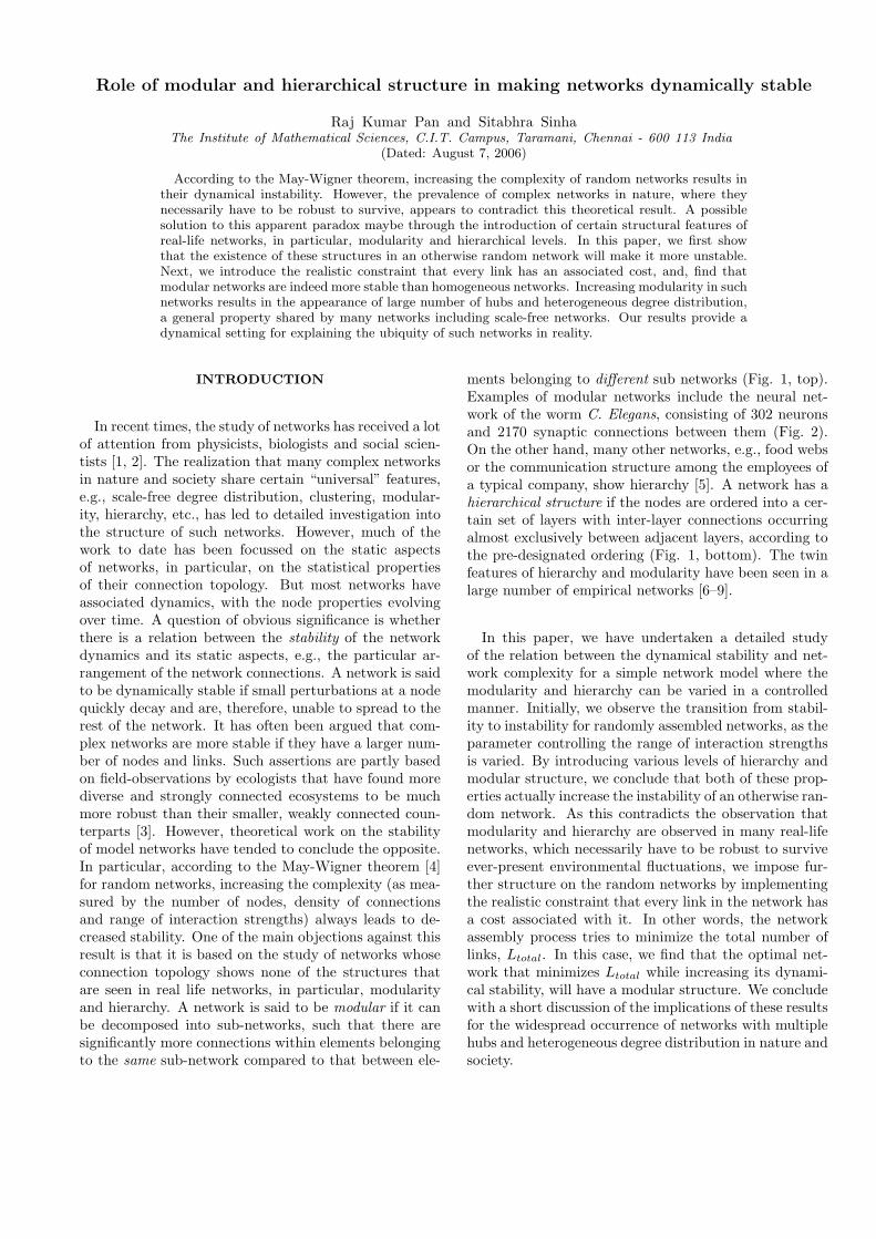
We introduce modular and hierarchical structure in anotherwise random network by dividing it into m modules(Fig. 3). This is done by generating the adjacency ma-trix A such that, the connectivity within each module,Cintra = ρ, is (in general) different from the connectivitybetween two modules belonging to the same hierarchi-

cal level, C(1)inter = rρ, where 0 ≤ r ≤ 1 is the parame-

ter controlling the degree of modularity in the network.Note that, r = 1 corresponds to the previously consid-ered case of a ER random network, while r = 0 corre-sponds to m disconnected random networks. Therefore,by changing r we can switch between completely modular(r = 0) and completely homogeneous (r = 1) networks.If two modules are separated by l levels in the hierar-chy, then the connectivity between these two modules

is C(l)inter = rlρ. The stochastic construction process of

our network model, along with the ability to vary mod-ularity (r) independent of hierarchy (l), makes it muchmore general than the deterministic model of hierarchicalmodular networks proposed by Ravasz & Barabasi [15].In addition, unlike in this previous study, P (k), the dis-tribution of the vertex degree k (the number of links as-sociated with a node), need not be scale-free. In fact, itturns out that the criterion for hierarchical modularitygiven in Ref. [15], namely, that the clustering for ver-tices of degree k, C(k) ∼ 1/k, is crucially dependent onthe scale-free degree distribution of the entire network.Thus, for a network having a different nature of P (k),e.g., the C. Elegans network which has an exponentialdegree distribution, the above criterion will indicate ab-sence of hierarchy or modularity even if such structuresdo exist. Also, in our model, a module is defined tonecessarily have more than one node, in contrast to a re-cent study where even a single node is considered to be amodule [16]. This is a significant difference, as the lattercriterion can lead to the identification of a set of discon-nected nodes as a “modular network”, when in fact thereis no network at all.

RESULTS

We look at the effect of modularity (r) and hierar-chy (l) on the stability of the model network, by ob-serving how changing their values affect the transitionfrom stability to instability as one of the network pa-rameters N,C, σ2 is varied. As mentioned before, for ERnetworks it is known that if N,C are fixed, then the criti-cal value of σ at which the transition to instability occursis σc ∼ 1/

√NC. Therefore, we check whether σc changes

with r and l. We arrange the network into hierarchicallevels, such that at each level every module can be splitfurther into a number of smaller modules; in the presentstudy, a module has been divided into two modules ateach level. Therefore, increasing the hierarchical level lresults in increasing the number of modules; this is to be

0.05 0.06 0.07 0.08 0.09 0.1 0.11 0.120

0.1

0.2

0.3

0.4

0.5

0.6

0.7

0.8

0.9

1

PS

tabi

lity

Variance, σ20.04 0.06 0.08 0.1 0.12 0.14 0.160

0.1

0.2

0.3

0.4

0.5

0.6

0.7

0.8

0.9

1

σ2

Pst

abili

ty

r = 0r = 0.1r = 0.5r = 1

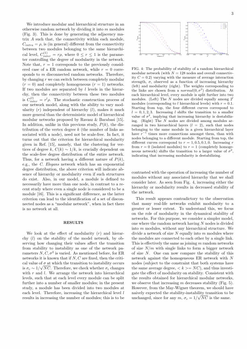
FIG. 4: The probability of stability of a random hierarchicalmodular network (with N = 128 nodes and overall connectiv-ity C = 0.2) varying with the measure of average interactionstrength, σ, observed as a function of increasing hierarchy(left) and modularity (right). The weights corresponding tothe links are chosen from a normal(0, σ2) distribution. Ateach hierarchical level, every module is split further into twomodules. (Left) The N nodes are divided equally among 2l

modules (corresponding to l hierarchical levels) with r = 0.1.Starting from top, the four different curves correspond tol = 0, 1, 2, 3. Increasing l shifts the transition to a smallervalue of σ2, implying that increasing hierarchy is destabiliz-ing. (Right) The N nodes are divided among modules ar-ranged in two hierarchical layers (l = 2), such that nodesbelonging to the same module in a given hierarchical layerhave r−1 times more connections amongst them, than withnodes belonging to a different module. Starting from top, thedifferent curves correspond to r = 1, 0.5, 0.1, 0. Increasing r

from r = 0 (isolated modules) to r = 1 (completely homoge-neous network) shifts the transition to a larger value of σ2,indicating that increasing modularity is destabilizing.

contrasted with the operation of increasing the number ofmodules without any associated hierarchy that we shallconsider later. As seen from Fig. 4, increasing either thehierarchy or modularity results in decreased stability ofthe network.

This result appears contradictory to the observationthat many real-life networks exhibit modularity to agreater or lesser extent. To understand this, we focuson the role of modularity in the dynamical stability ofnetworks. For this purpose, we consider a simpler model,one where the random network having N nodes is dividedinto m modules, without any hierarchical structure. Wedivide a network of size N equally into m modules wherethe modules are connected to each other by a single link.This is effectively the same as joining m random networksof size N/m with single links to form a bigger networkof size N . One can now compare the stability of thisnetwork against the homogeneous ER network with Nnodes (subject to the constraint that both systems havethe same average degree, < k >= NC), and thus investi-gate the effect of modularity on stability. Consistent withthe results obtained for hierarchical modular networks,we observe that increasing m decreases stability (Fig. 5).However, from the May-Wigner theorem, we should havenaively expected the stability-instability transition to beunchanged, since for any m, σc = 1/

√NC is the same.

4

−0.1 0 0.1 0.2 0.3 0.4

0

0.05

0.1

0.15

0.2

0.25

0.3

0.35

0.4

Re ( λ ) max

P{

Re

( λ

) max

}

m = 1

m = 2

m = 4

m = 8

0.02 0.025 0.03 0.035 0.040

0.2

0.4

0.6

0.8

1

σ2

Pst

abili

ty

FIG. 5: Probability distribution of the largest real-part ofeigenvalue for random network shown as a function of mod-ularity, m. The network consists of N = 256 nodes dividedequally into m modules where only a single undirected linkexists between two modules. The connectivity of the entirenetwork is C = 0.12 and the weights of the links are chosenfrom a normal(0, σ2) distribution with σ2 = 0.03. The insetshows the probability of stability for random networks as afunction of modularity. Increasing the modularity causes thetransition at a lower value of σ2, thus indicating increasingmodularity decreases stability for random networks.

To solve this apparent puzzle we first consider how thestability of a random network is affected by its size, N ,when the average degree (< k >= NC) is kept constant.As seen in Fig. 6, decreasing N causes the distribution ofthe largest real part of the eigenvalues Re(λ)max to be-come more long-tailed. As a result, close to the stability-instability transition region, the probability of Re(λ)max

having a positive value is slightly higher for networkswith smaller N . Thus, when we consider the statistics ofextremes, it is clear that close to the critical value of σc,the smaller networks are more likely to have instabilityinducing fluctuations compared to the larger networks.

Now we consider the fact that when a network of sizeN is split into m modules, the probability of stability ofthe entire network is decided by the probability of stabil-ity of the “most unstable” of the m modules of size N/m,ignoring the small additional effect of inter-modular con-nections. In other words, even if only one of the mod-ules is unstable, the entire network will be consideredunstable. Thus, the stability of the network of size N isdecided by randomly drawing m values from the distri-bution of Re(λ)max for network of size N/m. As pointedout before, the longer tail of the distribution for smallernetworks implies that it is now much more likely to ob-tain a positive value of Re(λ)max (especially in view ofthe m multiple drawings), than for the case of a homoge-neous network of size N . This explains why the modularnetwork is more unstable than the homogeneous network,

−0.4 −0.3 −0.2 −0.1 0 0.1 0.2 0.3

0

0.05

0.1

0.15

0.2

0.25

Re ( λ )max

P {

Re

( λ

) max

}

N = 256

N = 128

N = 32

N = 64

FIG. 6: Probability distribution of the largest real-part ofeigenvalue for ER random networks shown as a function ofsize N . The average degree < k >= 30, and the weights ofthe links are chosen from a normal(0, σ2) distribution with

σ2 = 0.03. The product√

NCσ2 is same for all the networks.

even though the two systems have the same total numberof links. Although the results shown here are for mod-ules connected to each other through a single link, theconclusion holds for the more general case of multipleinter-modular links (as seen in the hierarchical modularnetwork results for 0 ≤ r ≤ 1 presented above).

However, this does not answer our original questionof why we see modular networks in nature at all. Thisseems all the more difficult to answer when we realizethat modularity also increases the average path length ofa network, thereby increasing communication time withinthe network. Therefore, modular networks can be advan-tageous over other connection topologies only if, on in-troducing a certain important constraint usually imposedin real-life networks, modularity can actually turn out tobe stabilizing. A candidate for such a constraint is thelink cost [17], i.e., the cost involved in introducing eachadditional link in a network, e.g., in the case of airlinenetworks. Although the fastest network would be onewhere direct point-to-point flights connect every pair ofairports, such a system would be prohibitively costly aseach flight route would be expensive to maintain. In real-ity, therefore, one observes the existence of airline hubs,which acts as transit points for passengers arriving fromand going to other airports.

To see this constraint in terms of our model, we firstnote that a random network is distance minimizing butnot cost minimizing, when cost is measured as being pro-portional to the total number of links. This is because aminimum number of links (∼ N lnN) is required to en-sure that a random network is connected, i.e., there areno isolated sub-graphs [18].

It is easy to see that introducing the constraint ofleast cost (i.e., minimizing Ltotal) while requiring short-est communication in terms of average path length, leads

5

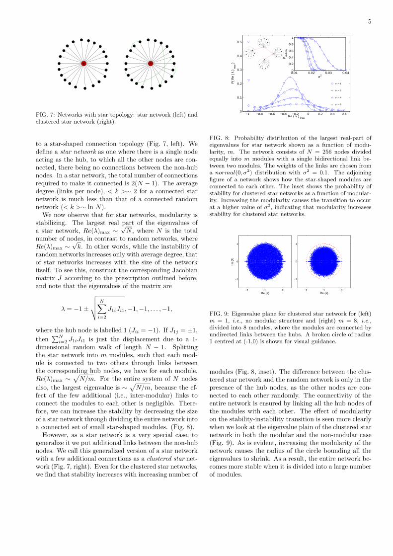
FIG. 7: Networks with star topology: star network (left) andclustered star network (right).

to a star-shaped connection topology (Fig. 7, left). Wedefine a star network as one where there is a single nodeacting as the hub, to which all the other nodes are con-nected, there being no connections between the non-hubnodes. In a star network, the total number of connectionsrequired to make it connected is 2(N − 1). The averagedegree (links per node), < k >∼ 2 for a connected starnetwork is much less than that of a connected randomnetwork (< k >∼ ln N).

We now observe that for star networks, modularity isstabilizing. The largest real part of the eigenvalues ofa star network, Re(λ)max ∼

√N , where N is the total

number of nodes, in contrast to random networks, whereRe(λ)max ∼

√k. In other words, while the instability of

random networks increases only with average degree, thatof star networks increases with the size of the networkitself. To see this, construct the corresponding Jacobianmatrix J according to the prescription outlined before,and note that the eigenvalues of the matrix are

λ = −1 ±

√

√

√

√

N∑

i=2

J1iJi1,−1,−1, . . . ,−1,

where the hub node is labelled 1 (Jii = −1). If J1j = ±1,

then∑N

i=2 J1iJi1 is just the displacement due to a 1-dimensional random walk of length N − 1. Splittingthe star network into m modules, such that each mod-ule is connected to two others through links betweenthe corresponding hub nodes, we have for each module,Re(λ)max ∼

√

N/m. For the entire system of N nodes

also, the largest eigenvalue is ∼√

N/m, because the ef-fect of the few additional (i.e., inter-modular) links toconnect the modules to each other is negligible. There-fore, we can increase the stability by decreasing the sizeof a star network through dividing the entire network intoa connected set of small star-shaped modules. (Fig. 8).

However, as a star network is a very special case, togeneralize it we put additional links between the non-hubnodes. We call this generalized version of a star networkwith a few additional connections as a clustered star net-work (Fig. 7, right). Even for the clustered star networks,we find that stability increases with increasing number of

−1 −0.8 −0.6 −0.4 −0.2 0 0.2 0.4 0.60

0.1

0.2

0.3

0.4

0.5

Re ( λ ) max

P{ R

e ( λ

) max

}

m = 8

m = 4

m = 2

m = 1

0.01 0.02 0.03 0.040

0.2

0.4

0.6

0.8

1

σ2

Pst

abili

ty

FIG. 8: Probability distribution of the largest real-part ofeigenvalues for star network shown as a function of modu-larity, m. The network consists of N = 256 nodes dividedequally into m modules with a single bidirectional link be-tween two modules. The weights of the links are chosen froma normal(0, σ2) distribution with σ2 = 0.1. The adjoiningfigure of a network shows how the star-shaped modules areconnected to each other. The inset shows the probability ofstability for clustered star networks as a function of modular-ity. Increasing the modularity causes the transition to occurat a higher value of σ2, indicating that modularity increasesstability for clustered star networks.

−2 −1 0

−1

0

1

Im (

λ)

Re (λ)−2 −1 0

−1

0

1

Re (λ)

FIG. 9: Eigenvalue plane for clustered star network for (left)m = 1, i.e., no modular structure and (right) m = 8, i.e.,divided into 8 modules, where the modules are connected byundirected links between the hubs. A broken circle of radius1 centred at (-1,0) is shown for visual guidance.

modules (Fig. 8, inset). The difference between the clus-tered star network and the random network is only in thepresence of the hub nodes, as the other nodes are con-nected to each other randomly. The connectivity of theentire network is ensured by linking all the hub nodes ofthe modules with each other. The effect of modularityon the stability-instability transition is seen more clearlywhen we look at the eigenvalue plain of the clustered starnetwork in both the modular and the non-modular case(Fig. 9). As is evident, increasing the modularity of thenetwork causes the radius of the circle bounding all theeigenvalues to shrink. As a result, the entire network be-comes more stable when it is divided into a large numberof modules.

6

CONCLUSION

In this paper we have shown that, although hierar-chy and modularity in random networks are destabiliz-ing, when we introduce real-life constraints, such as acost per link, modular networks turn out to be stabiliz-ing. Note that, an alternative way of stating this is thatstable networks will exhibit multiple hubs and will havea heterogeneous degree distribution. Many types of net-works, including scale-free networks [19], can be seen asspecial cases of this general criterion. Therefore, by intro-ducing dynamical considerations along with a link-costconstraint, we can understand the large-scale occurrenceof such networks in the natural and social world.

[1] M. E. J. Newman, SIAM Review 45, 167 (2003).[2] R. Albert and A.-L. Barabasi, Rev. Mod. Phys. 74, 47

(2002).[3] C. S. Elton, The Ecology of Invasions by Animals and

Plants, Methuen, London (1958).[4] R. M. May, Stability and Complexity in Model Ecosys-

tems, Princeton University Press, Princeton, NJ (1973).

[5] T. Hogg, B. A. Huberman and J. M. McGlade, Proc.Roy. Soc. Lond. B 237, 43 (1989).

[6] E. Ravasz, A. L. Somera, D. A. Mongru, Z. N. Oltvai andA.-L. Barabasi, Science 297, 155 (2002).

[7] R. V. Sole and A. Munteanu, Europhys. Lett. 68, 170(2004).

[8] P. Holme, M. Huss and H. Jeong, Bioinformatics 19, 532(2003).

[9] A. E. Krause, K. A. Frank, D. M. Mason, R. U. Ulanow-icz and W. W. Taylor, Nature 426, 282 (2003).

[10] V. K. Jirsa and M. Ding, Phys. Rev. Lett. 93, 070602(2004).

[11] S. Sinha and S. Sinha, Phys. Rev. E 71, 020902(R)(2005).

[12] S. Sinha, Physica A 346, 147 (2005).[13] M. Brede and S. Sinha, arxiv cond-mat/0507710 (2005).[14] P. Erdos and A. Renyi, Publ. Math. Inst. Hung. Acad.

Sci., Ser. A 5, 17 (1960).[15] E. Ravasz and A.-L. Barabasi, Phys. Rev. E 67, 026112

(2003).[16] E. A. Vaiano, J. M. McCoy and H. Lipson, Phys. Rev.

Lett. 92, 188701 (2004).[17] N. Mathias and V. Gopal, Phys. Rev. E. 63, 02117

(2001).[18] B. Bollobas, Random Graphs, Cambridge University

Press, Cambridge (2001).[19] A.-L. Barabasi and R. Albert, Science 286, 509 (1999).