role of textiles and paper for stabilizing the … · we take the influence of the indoor materials...

KATHOLIEKE UNIVERSITEIT

LEUVEN

KATHOLIEKE UNIVERSITEIT LEUVEN FACULTEIT INGENIEURSWETENSCHAPPEN DEPARTEMENT BURGERLIJKE BOUWKUNDE AFDELING BOUWFYSICA KASTEELPARK ARENBERG 40 B-3001 HEVERLEE

ROLE OF TEXTILES AND PAPER FOR

STABILIZING THE INDOOR ENVIRONMENT

Promotor:

Prof. Dr. J. Carmeliet Derluyn Hannelore

E2006 Eindwerk voorgedragen

tot het behalen van de

graad van burgerlijk

ingenieur

Copyright ©2006, K.U.Leuven. Alle rechten voorbehouden. Niets uit deze uitgave mag worden verveelvoudigd, opgeslagen in een geautomatiseerd gegevensbestand, of openbaar gemaakt, in enige vorm of op enige wijze, hetzij elektronisch, mechanisch, door fotokopiëren, opnamen, of op enige andere manier, zonder voorafgaandelijke schriftelijke toestemming van de auteur. De auteur geeft de toelating deze eindverhandeling voor consultatie beschikbaar te stellen en delen ervan te kopiëren voor eigen gebruik. Elk ander gebruik valt onder de strikte beperkingen van het auteursrecht; in het bijzonder wordt er gewezen op de verplichting de bron uitdrukkelijk te vermelden bij het aanhalen van resultaten uit deze eindverhandeling. Leuven, juni 2006 All rights reserved. No part of this publication may be reproduced, stored in a retreival system, or transmitted, in any form or by any means, electronic, mechanical, photocopying, recording, or otherwise, without the prior written permission of the author. This publication can be made available for consultation. Photocopying for private use is permitted. Any other use strictly submitted to copyright law. Every quote of results from this publication must contain a reference to it.

Dankwoord

Vijf fantastische jaren in Leuven zijn voorbij gevlogen, en ik ben dan ook blij om hier

de kroon op het werk van deze voorbije vijf jaar aan u voor te stellen, mijn eindwerk.

Een eindwerk schrijf je nooit alleen, maar de energie van vele personen zit erin vervat

en daarom wil ik graag mijn woord van dank uitdrukken aan alle mensen die dit

eindwerk en ook mijn studieperiode in Leuven tot een prachtige ervaring hebben

gekneed.

Allereerst wil ik mijn promotor bedanken, Professor Carmeliet. Dank voor de

tweewekelijkse brainstormsessies, waarbij ik telkens nieuwe ideeën en mogelijkheden

opdeed om een volgende stap in het onderzoek te zetten. Dank ook voor het nalezen en

verbeteren van de tekst. Also I want to thank Professor Derome for her support and

interest in my master thesis, for her remarks and help in finding the answers to my

questions. Graag bedank ik ook Hans Janssen voor de hulp bij berekeningen en het

simuleren met HAMFEM en het mee helpen zoeken naar oplossingen. Ook Professor

Roels wil ik bedanken, voor de uitleg bij het programma ROOMHAM.

Een tweede dankwoord is gericht aan mijn ouders en broer. Papa, dank je voor de vele

computerhulp en de ideeënwisselingen en je rustige energie, die mij de voorbije vijf jaar

altijd vooruit hielpen. Moeke, dank je voor je eeuwig positivisme, voor het geven van je

zonnige energie, om er voor mij te zijn. Pieter-Jan, dank je voor je luisterend oor en de

ontspannende lachmomenten die je altijd weet te creëren.

Een laatste dankwoord is gericht aan de vrienden. Allereerst de mensen die de voorbije

vijf jaar toch wel echt speciaal gemaakt hebben: dank je vrienden van Caprabo voor de

vele mooie burgiemomenten! Dank ook aan Inge, voor je onvoorwaardelijke

vriendschap. En als laatste richt ik ook aan de Induce-dansers en de vriendinnen uit

Roeselare mijn welgemeende dank.

Hannelore Derluyn

1

General introduction

In buildings, it is very important to maintain a stable indoor environment. This means to

create a comfortable temperature and relative humidity in the indoor space. This thesis

focuses on the second requirement: achieving a good moisture control of the indoor

environment.

It is very important to obtain a moderate relative humidity in indoor spaces. A too high

relative humidity and too large fluctuations in relative humidity, for example due to

temperature changes or moisture sources (people, plants), may cause damage to

buildings and furniture. E.g. mould growth forming, structure deformations (dilatation

and shrinking), cracks. So the durability of a building can strongly decrease due to

moisture problems.

The humidity has also an influence on the comfort and the health of the occupants in the

building. Too high or too low relative humidities and large fluctuations in relative

humidity are experienced as unpleasant: mould and condensation on surfaces due to a

high relative humidity or static electricity due to a low relative humidity aren’t desired.

A high relative humidity aids the growth of bacteria, which leads to health problems.

In the indoor environment there are a lot of materials acting as moisture buffers. Not

only the building materials, but also furnishing materials, books and magazines, cloths

of curtains, pillows, blankets,… contribute to the moisture buffering capacity of rooms.

Recent research (Svennberg, Rode) shows that those materials have an important impact

on the moisture buffering performance of a room and that more properties and

information need to be determined to understand their influence.

In this report we focus on the role that paper and textiles can play in the stabilisation of

indoor climates.

Knowing more about the buffering materials will make it possible to simulate the

moisture buffering in rooms better and more correct. Climatisation installations can be

dimensioned in order to obtain a stable indoor environment by using simulations. When

we take the influence of the indoor materials into account, we expect that the load on

2

the installations will decrease. In this way the energy costs for climatisation installations

can be reduced, because the indoor materials give us buffering ‘for free’.

Research on the behaviour of indoor materials like paper and textiles will consequently

lead to a better understanding of the moisture buffering and relative humidity

fluctuations in living rooms, bedrooms, … of dwelling-houses.

This research on paper and textiles can especially be interesting for buildings like musea

and libraries. They require a thorough attention for their indoor climate, because of the

importance of a good preservation of art objects and books. Therefore it is interesting to

investigate how paper and books react on moisture. Fabrics can help to buffer the

humidity fluctuations e.g. in the form of curtains and wall and floor covering.

The research on textiles is not only interesting in building physics, but can also be used

in the development of clothes like for instance sportswear, where the buffering of sweat

is an important issue.

This report lies within the framework of the international IEA (International Energy

Agency) project Annex 41, Whole Builing Heat, Air and Moisture response.

3

Abstract Indoor environmental conditions can be regulated by moisture sorption of hygroscopic

materials. Being made of organic fibres, paper and textiles are quite hygroscopic, and

the potential contribution to the regulation of indoor environments due to the presence

of newspapers, magazines, books, curtains, pillows or carpets should be analysed.

At first a literature review has been done, where general characteristics of paper and

textiles are discussed and data from literature can be found. Secondly, experimental

work was done, i.e. microscopic images, material properties and dynamic behaviour.

Tests were performed on book samples, using two types of paper, and on cotton. The

data collected out of literature and measurements are used in the modelling calculations.

This thesis investigates which parameters, e.g. water vapour permeability, moisture

capacity, active area, etc., play an important role, and presents an understanding of the

processes of moisture buffering in a book and in a textile sheet.

A book is modelled as a multilayered air-paper system. The model focuses on moisture

transport through the fore-edge or the top-edge of a book, i.e. with vapour transport

parallel to the pages of the book. The present study looks at the impact of the type of

paper and the fraction of paper, taken to be the ratio of the paper volume to the volume

of the book. A newsprint paper and a magazine type of paper are studied, and two paper

fractions, for a tight and a somewhat loose binding, are analysed. Eventually, it will be

shown that a book can be modelled as ‘one material’, with properties determined by the

paper fraction and the kind of paper.

For textile, the study focuses on cotton. A cotton sheet is thoroughly measured by

microscopic research. Out of the measurements a mesh of the cotton structure is

developed. Modelling the moisture buffering of the textile sheet shows the importance

of the air holes in between the woven structure on the moisture buffering effect. The

moisture content and capacity of the cotton yarns itself can be expressed in terms of the

cotton fraction, i.e. the ratio of the yarns volume to the total volume of the cotton fabric.

The vapour permeability of the cotton yarns is determined with the model.

4

In a last part of this thesis, an attempt to model the influence of paper and cotton on the

moisture buffering in a room is discussed. Textile will help to regulate the moisture

variation especially when there are peaks in the moisture production. Books will reduce

the relative humidity fluctuations considerably when the accessible surface is large

enough, e.g. in offices. Future work on this topic should be performed by building a

test room and making comparisons between experimental measurements and modelling

results.

5

Table of contents

Nomenclature ..................................................................................................................9

PART 1 PAPER .........................................................................................................11

1 Literature review...................................................................................................11

1.1.1 The material paper...................................................................................11

1.1.2 Basic properties of paper .........................................................................13

1.1.3 Moisture in paper.....................................................................................14

1.1.3.1 Relative humidity and moisture content .........................................14

1.1.3.2 Interaction of water with fibers .......................................................15

1.1.3.3 Hysteresis and dynamic behaviour .................................................16

1.2 Moisture properties of paper ...........................................................................18

1.2.1 Sorption isotherms...................................................................................18

1.2.2 Vapour resistance factor ..........................................................................22

1.2.3 Families of paper .....................................................................................23

2 Experimental work ...............................................................................................24

2.1 Micro-meso structure ......................................................................................24

2.1.1 SEM images.............................................................................................24

2.2 Material properties ..........................................................................................27

2.2.1 Basic properties of the paper ...................................................................27


2.2.3 Vapour permeability................................................................................33

2.3 Dynamic behaviour .........................................................................................37

2.3.1 Definitions ...............................................................................................37

2.3.2 Test setup.................................................................................................37

2.3.3 Experimental determination of surface mass transfer coefficients..........40

2.3.4 Test results...............................................................................................40

3 Modelling of the hygroscopic behaviour of books..............................................44

3.1 Theory .............................................................................................................44

3.2 Preliminary simulations ..................................................................................45

3.2.1 Modelling in HAMFEM..........................................................................45

3.2.2 The model................................................................................................46

6

3.2.3 Penetration profile ...................................................................................48

3.2.4 Influence surface coefficient and air layer thickness ..............................49

3.3 Two-dimensional modelling and effective permeability ................................50

3.3.1 Model 1: two-dimensional model of the real book at mesoscale

(Figure 19)...............................................................................................................50

3.3.2 Model 2: two-dimensional model of the effective book at macroscale

(Figure 22)...............................................................................................................50

3.3.3 Initial, boundary conditions, material properties.....................................51

3.3.4 Results .....................................................................................................51

3.4 Discussion .......................................................................................................53

3.4.1 Moisture capacity of book .......................................................................53

3.4.2 Moisture permeability of book ................................................................54

3.4.3 Moisture buffering of books....................................................................54

3.4.4 A varying vapour resistance factor for paper ..........................................57

3.5 Modelling the dynamic behaviour of the experimental tested books .............58

3.5.1 Analytical description of the dynamic behaviour of books.....................58

3.5.2 Applying effective book model on experimental results of dynamic

behaviour of books..................................................................................................61

3.5.2.1 Expected results versus analytical description................................61

3.5.2.2 Test results versus book model and analytical description .............63

3.5.2.2.1 Magazine .......................................................................................65

3.5.2.2.1.1 Magazine high paper fraction.................................................66

3.5.2.2.1.2 Magazine low paper fraction..................................................67

3.5.2.2.2 Telephone book.............................................................................69

3.5.2.2.2.1 Telephone book high paper fraction ......................................70

3.5.2.2.2.2 Telephone book low paper fraction........................................71

3.5.2.3 Discussion .......................................................................................72

7

PART 2 COTTON .....................................................................................................76

1 Literature review...................................................................................................76

1.1

1.2

2

2.1

2.2

3

3.1

Textile .............................................................................................................76

1.1.1 Textile fabrics..........................................................................................76

1.1.2 Cotton ......................................................................................................77

1.1.3 Density of textiles....................................................................................78

1.1.4 Moisture in textiles ..................................................................................79

1.1.4.1 Absorption of moisture ...................................................................79

1.1.4.2 Rate of absorption of moisture........................................................80

1.1.4.3 Theories of moisture sorption .........................................................81

Moisture properties of textiles. .......................................................................83


1.2.2 Vapour resistance factor ..........................................................................87

1.2.3 Families of textiles ..................................................................................88

Experimental work ...............................................................................................89

Micro-meso structure ......................................................................................89

2.1.1 SEM and microscope images ..................................................................89

Material properties ..........................................................................................93

2.2.1 Basic properties of the cotton ..................................................................93

2.2.2 Sorption isotherm ....................................................................................94

2.2.3 Vapour permeability................................................................................95

Modelling of the hygroscopic behaviour of a textile fabric...............................98

The model .......................................................................................................98

3.2 Three dimensional modelling and effective permeability...............................99

3.3 Penetration profile.........................................................................................100

3.4 Conclusions...................................................................................................102

8

PART 3 PAPER&COTTON...................................................................................103

1 Modelling moisture buffering in a room...........................................................103

1.1

1.1

1.1.3

GENERAL CONCLUSION.......................................................................................110

FUTURE WORK ........................................................................................................112

List of figures ...............................................................................................................114

Simulations with ROOMHAM .....................................................................103

1. Material input ........................................................................................104

1.1.2 Simulations ............................................................................................105

1.1.2.1 Moisture production with peaks....................................................106

1.1.2.2 Constant moisture production during occupation .........................107

1.1.2.3 Concluding observations...............................................................108

Discussion..............................................................................................108

List of tables.................................................................................................................118

References ....................................................................................................................120

9

Nomenclature

Symbols A surface m² bm moisture effusivity kg/(m²s0,5Pa) d thickness m D moisture diffusivity m²/s gv vapour flow density rate kg/(m²s) Gvp vapour production kg/s, g/h m mass kg mdry dry mass kg mdelta permeability correction factor for calculating the

vapour permeability of a book -

meffus effusivity correction factor for calculating the effusivity of a book

-

n ventilation rate 1/h, 1/s p barometric pressure Pa pc capillary pressure Pa pv vapour pressure Pa pv,sat saturation vapour pressure Pa q vapour flow kg/(m²s) qbuf water vapour exchange with buffering surface kg/(m²s) R gas constant J/kgK RH relative humidity % Sl degree of saturation (by liquid) - t time s ta thickness air layer m tp thickness paper sheet m T temperature K V volume m³ W water vapour permeance kg/(m²sPa) w moisture content kg/m³ or kg/kg wa adsorption moisture content kg/m³ or kg/kg wd desorption moisture content kg/m³ or kg/kg wsat saturation moisture content (RH=100%) kg/m³ or kg/kg β surface mass transfer coefficient s/m δ vapour permeability s φ relative humidiy -

totφ total porosity m³/m³ oφ open porosity m³/m³

aΨ air fraction -

pΨ paper fraction - μ vapour resistance factor - θ temperature °C ρ density kg/m³

vρ water vapour concentration kg/m³ ξ moisture capacity kg/m³

10

Suffixes

a air a adsorption b book c cotton d desorption e environment / outside f fiber fws solid part of fiber wall fwp pores in fiber wall fl fiber lumen i inside l liquid p paper sat saturation v vapour

11

PART 1 PAPER

1 Literature review

The main source for the literature review is based on the book ‘Paper physics’.

Additional information was found on the website www.paperonweb.com and the

website of the papermaking company UPM w3.upm-kymmene.com.

1.1.1 The material paper

The properties of a paper are mainly determined by its fibers and the bonding between

them. The fiber properties depend on the kind of wood and the pulping and

papermaking process. Usually the paper is made of wood fibers, but in specialty papers

nonwood fibers are also commonly used.

Wood consists of cellulose and hemicellulose, bonded by lignin. Cellulose and

hemicellulose are polymers, cellulose made from glucose, hemicellulose from other

sugars. The lignin provides the

strength of the wood. Wood

fibers consist of a cell wall

which encloses the lumen. The

cell wall of one fiber is

composed of micro fibrils,

surrounded by a matrix of

amorphous material, primarily

hemicelluloses and lignin. The main properties of a fiber are its length, the fiber

coarseness (dry fiber mass per unit length) and the basis weight (fiber coarseness

divided by fiber width). The total fiber length is 10-100 m for every cm² of a typical

paper sheet, which corresponds to 10 000-100 000 fibers. The basis weight ranges from

3-10 g/m². The fibers of one tree can differ when there is a seasonal variation in growth

and therefore in fiber density and dimensions.

Figure 1. Structure of cellulose. (Wikipedia)

Apart from the wood components in paper, also other substances, fillers, are added. E.g.

kaolin, which gives a glossy finish to a paper sheet.

http://nl.wikipedia.org/wiki/Afbeelding:Cellulose.png�

12

In the papermaking process, pulping, bleaching and beating affect the final paper

properties. Pulping is the process in which the wood is broken up into wood fibers. Two

basic pulp classes are bleached kraft pulp and mechanical pulp. Bleached kraft pulp or

chemical pulp is formed by cooking the wood chips in a chemical solution to remove

the wood’s natural binding agent lignin. In this way, the wood is disintegrated into

fibers. In mechanical pulping, fibers are separated mechanically. The first step is to

press the tree trunks against a rotating grindstone. The wood chips are then put into

refiners, where the fibers are separated between two rotating disks.

Depending on the pulping process, the paper properties differ. For example, newspaper

often consists of pure mechanical pulp and copy paper of pure chemical pulp. Mixtures

of mechanical and chemical pulp are used in printing papers and multiply boards. In

mechanical pulps, the lignin content is approximately 30%, in chemical pulps almost

zero. Especially in mechanical pulping, fiber particles are generated. 20% to 40% by

weight of mechanical pulp are fiber particles, for chemical pulp this is less than 10%.

Fiber particles have a median size of a few micrometers and consist mainly of cellulose,

hemicellulose and lignin. The largest fiber particles are fiber fragments, the smallest are

fibrils or parts of fibrils. In mechanical pulps, the considerable amount of fiber particles

influences strongly the properties of the fiber network. In chemical pulp this influence is

limited as the content is much lower. The fiber particles have a very large surface area

because of their small particle size and therefore improve the bonding between fibers.

When drying, most of the particle surface is bonded to fibers. Chemical pulp particles

bond almost completely and all free surface is lost. Mechanical fiber particles retain

some of their free surface and can so influence the paper properties.

Pulp often undergoes bleaching. Bleaching whitens the pulp, enhances brightness and

eliminates impurities. Bleaching is done with bleaching chemicals, e.g. chlorine, ozone,

oxygen or hydrogen peroxide.

Chemical pulp is usually beaten to ameliorate the mechanical properties of the paper.

The structure of the fiber wall and surface is loosened by the beating process; this is

called respectively internal and external fibrillation. Internal fibrillation leads to a partial

delamination. This causes an increase of the swelling degree and flexibility of the wet

fiber wall. Due to beating also fragments can break from the fiber wall.

The similar effect is obtained by mechanical pulping.

The bonding between paper fibers is primarily due to hydrogen bonds. The hydrogen

bonds in cellulosic materials as paper form when a hydroxylic group (OH) bonds to an

13

electronegative element such as oxygen. The hydrogen bonds are not only found

between the fibers of paper, but also between the fibrils of the fiber wall and between

the glucose units in the cellulose.

1.1.2 Basic properties of paper

The properties characterizing paper on macroscopic level are the density, the porosity

and the thickness. These properties may vary because of the irregularity of the paper

thickness and the variability in the density of fibers.

The density ρ [kg/m³] is the ratio of the weight per unit surface bw [kg/m²] and the

thickness d [m] of the paper.

The porosity φ [m³/m³] is the ratio of the pore volume to the total volume. The total

porosity is given by the formula

fws

fwstot V

Vρρ

φ −=−= 11 (1)

with V the total volume of the paper sheet [m³], which consists of the volume of the

solid part of the fiber wall Vfws, the volume of the pores in the fiber wall , the

volume of the fiber lumen Vfl and the remaining volume in between the fibers Vr. Thus

. ρ is the density of the paper sheet and ρfws the density of the

solid fiber wall. ρfws is assumed to be 1500 kg/m³ (this is so for perfect cellulosic

fibrils).

fwpV

rflfwpfws VVVVV +++=

When transporting for example inert liquids trough paper, the pore volume inside the

fiber, the lumen, does not contribute to the transport. If we want to take this into

account, an open porosity needs to be defined. This is the porosity contributing to the

fluid transport and is expressed by the formula:

f

flfwso V

VVρρφ −=

+−= 11 . (2)

The density of the fiber ρf has a value of 1000 – 1100 kg/m³.

The porosity varies according to the paper composition (fibers, fillers, etc.), the

papermaking method, the paper furnish and the beating level of the paper. All these

parameters lead to the fact that it is almost impossible to determine the porosity

experimentally.

14

The thickness is difficult to measure. Due to the surface roughness, there are many

variations on a very small scale, which makes it hardly impossible to determine the

‘true’ thickness. As a consequence, a definition of ‘true’ density cannot be given, it will

always be an ‘apparent’ thickness and density.

The density of paper varies from 600-690 kg/m³ for newsprint paper to 780 kg/m³ for

fine paper, and up to 1150 kg/m³ for coated super calendared paper. Newsprint paper

thickness may vary from 60 to 80 microns; office paper is around 100 to 110 microns.

The porosity of paper can be as high as 70%.

In the z-direction (the thickness direction) of a paper sheet, there is a distribution of the

structural components such as fibers and fillers and a variation of the mass density. Due

to the small thickness of paper, it is difficult to measure those distributions. They are

determined by the papermaking method. Typical examples are sheets where the middle

layers have low density and the surface layers have high density. This gives good

smoothness, printability and bending stiffness. The same effect is achieved by a high

concentration of fiber particles at the sheet surfaces. When fillers are used, the

distribution in the z-direction is essential to get the desired paper properties.

1.1.3 Moisture in paper

In equilibrium, the moisture content of paper depends on the relative humidity and the

temperature of the environment. A humid and cold environment gives the highest

relative humidity. The moisture content depends on the preceding states of moisture

content, it is history-dependent. The pulp composition influences the hygroscopic

behaviour of a paper: the chemical interaction of water molecules with the cellulosic

fiber wall influences the moisture content as well as the internal and external fibrillation

and fiber particles content of the pulp. When the water is removed during paper drying,

the fiber wall structure changes. These changes can be irreversible, depending on the

type of pulp.

1.1.3.1 Relative humidity and moisture content

The relative humidity, RH [-] , of air gives the ratio of the amount of water vapour in air

to the maximal amount (saturation). The higher the temperature is, the higher the

saturation water vapour content is. RH is often defined by the water vapour pressure, it

is the ratio between the ambient vapour pressure to the saturation vapour pressure:

15

satv

v

ppRH

,

.100= (3)

The vapour pressure pv [Pa] is related to the vapour concentration ρv [kg/m³] by the

ideal gas law:

TRp vv ..ρ= (4)

with T the temperature in Kelvin and R the gas constant of water vapour (462 J/kgK).

The saturation vapour pressure can be expressed by

)3,237

.269,17exp(.5,610, θθ

+=satvp , with θ the temperature in °C. (5)

The moisture content of paper is the ratio of absorbed water divided by the mass of dry

paper. In equilibrium, the moisture content depends on the relative humidity and the

temperature of the environment. Increasing the temperature or decreasing the relative

humidity leads to a decrease in moisture content. In normal conditions the moisture

content of paper is between 2 and 12%. At a constant RH the moisture content is quite

insensitive to temperature. Except in humid conditions, a temperature change of more

than ±10°C is necessary before the moisture content changes significantly.

The hygroscopic behaviour of paper is determined by the papermaking pulp.

Mechanical pulps are often more hygroscopic than chemical pulps. The fiber particles

of mechanical pulps are the important factor here. In chemical pulps, the amounts of

amorphous cellulose and hemicellulose are more important.

1.1.3.2 Interaction of water with fibers

Papermaking fibers absorb water as free water or as bonded water. Free water can be

found in the pores between fibers or in the lumen of fibers. Bonded water can be found

in the pores of the fiber wall or it can be chemically bonded to the hydroxylic and

carboxylic acid groups in fibers. Only the water bonded to hydroxyl groups remains in

fibers at moisture contents below 20%. When the moisture content is 20%-40% or

RH>90% at 23°C, the pores in the fiber wall become active. Free water can only play a

role at still higher moisture contents.

Paper absorbing water makes the fibers swell because the water molecules penetrate

between the hydrogen-bonded fibrils in the fiber wall. The amount of bonded water

increases, and the degree of internal bonding of the fiber wall decreases. Desorption

leads to the opposite.

16

Beating of a chemical pulp increases swelling because of the increase of the

delamination of the fiber wall. Also in chemical pulps, the phenomenon of hornification

can occur. This means that there is an irreversible loss of the water absorption capacity

of the pulp in drying. When we rewet the paper, the pulp absorbs less water than before

drying.

The water attaches to the hydroxyl groups and so the chemical composition of the pulp

has an important influence on the moisture content and the swelling. Cellulose and

hemicelluloses contain three OH-groups per six carbon atoms. Lignin contains only one

or two OH-groups per 10 carbon atoms. The availability of the OH-groups is also

important. In amorphous cellulose, the internal bonding is weak and OH-groups are

readily available for water. In crystalline cellulose, bonding is stronger and thus the

availability of OH-groups is lower. It can be concluded that amorphous cellulose and

hemicelluloses promote water absorption, lignin nearly inhibits absorption.

1.1.3.3 Hysteresis and dynamic behaviour

Hysteresis is the phenomenon that the moisture content at a certain relative humidity is

different in absorption, coming from dry conditions, than in desorption, coming from

humid conditions. Depending on the history, the moisture content can be anywhere

between the two boundary curves. We get the boundary curves when we start from

perfectly dry paper and go to saturation and vice versa.

The hysteresis effect is connected to the hygroscopic nature of wood fibers. To remove

water from fibers, thermal energy (heat of desorption) is necessary. When the fibers

absorb water, heat of absorption releases. So the heat of sorption leads to a difference in

water vapour pressure, this is in RH, between absorption and desorption.

Several mechanisms can explain hysteresis. In the domain theory it is said that

hysteresis arises from independent microscopic domains that can be in two states,

‘sorbing’ or ‘nonsorbing’. The domain state switches upon absorption or desorption of

water. It is necessary to cross an energy barrier to cause a switch.

Others argue that the shape of the microscopic domains controls hysteresis. The

domains have different sizes and capillary pressure causes small domains to absorb

water more readily than large domains. This is called the bottleneck theory.

The availability of hydroxyl groups, which bind the water, can also explain the

hysteresis effect. It is so that the cellulose molecules form groups, micelles, which are

17

weakly bonded to each other. When water is absorbed, some of the bonded hydroxyl

groups become free to associate with more water. In desorption, the opposite occurs.

A last explanation is the occurrence of swelling stresses and the irreversible plastic

deformations they cause. These stresses arise in the fiber wall because crystalline

cellulose does not swell (and the non-crystalline cellulose regions do). The

deformations are reversible (elastic) at small amounts of absorbed water. At larger

amounts of water, the swelling stress may exceed a yield limit and causes plastic

deformations. Due to this, the weak bond between the micelles can be broken and free

more hydroxyl groups to absorb water.

Dynamic phenomena act when there is a sudden change in the external conditions. The

moisture content cannot adapt immediately to the new situation. In ordinary diffusion,

the moisture content would change proportionally to the square root of time. The

diffusion time should be proportional to the square of the weight per unit surface. This

ordinary diffusion approach would require that the boundary conditions of the paper

sheet were constant. However, if we consider a boundary layer at the sheet surface, this

is not the case. The local humidity and temperature in the boundary layer are different

from the ambient conditions and the ordinary solution doesn’t apply anymore.

The conditions in the boundary layer are determined by the sorption heat. In the case of

absorption, temperature increases and RH decreases in the boundary layer. This leads to

a retardation of the diffusion process because the paper sheet sees a lower RH than the

ambient RH. In the case of desorption, the opposite process takes place. So, the

resulting diffusion process is slower than it would be if only the diffusivity of water

vapour would determine the sorption rate.

18

1.2 Moisture properties of paper

In literature, a lot of measurements on sorption isotherms of paper can be found. The

sources for the data on paper, used in this report, are the Annex XIV – Catalogue of

Material Properties (Kumaran, 1996) and some papers about the material paper

(Chatterjee, 2001; Gupta & Chatterjee, 2003; Motta Lima et al, 2003; Ramarao et al,

2003). The data can be found in Appendix 1.

The characteristics of the paper materials found in literature are given in Table 1.

Table 1. Material characteristics of paper.

name thickness

(mm)

mass per m²

(kg/m²)

density

(kg/m³)

periodical (Knack) 0,07 (estimation) 0,047 671

newspaper (De Standaard) 0,056 (estimation) 0,041 729

wallpaper 1 (textile) 0,425 0,291 685

wallpaper 2 (vinyl) 0,325 0,216 665

wallpaper 3 (textile) 0,7 0,333 476

wallpaper 4 (vinyl) 0,45 0,212 471

wallpaper 5 (paper) 0,28 0,168 600

wallpaper 6 (paper) 0,28 0,151 539

Bleached kraft paperboard

(BKP) 0,35 0,23 663

KLABIN-PR KLAPAK 0,75 (estimation) 0,265 353

(commercial liquid package

paper)

1.2.1 Sorption isotherms

Based on the literature data, the adsorption isotherms are described by a curve of the

van Genuchten type:

( )( )( ) nn

nsat aww

−

+=1

ln.1 φ (6)

with w the moisture content in kg/m³, φ the relative humidity; wsat is the maximal

19

moisture content at φ =1. a and n are parameters. The parameters wsat, a and n can be

found in Table 2. The figures 2 and 3 show a graphical representation of the curve

fitting.

The moisture capacity is the derivative of the moisture content to the relative humidity:

( )( )( ) ( )( )φ

φφφ

ξ aanan

nww nnn

nsat .ln...ln.1.1. 111

−−⎟⎠⎞

⎜⎝⎛ −

+⎟⎠⎞

⎜⎝⎛ −

=∂∂

= (7)

The moisture capacity is determined using the fitting parameters of Table 2. The result

is given in the figures 4 and 5.

Table 2. The parameters for the analytical fit of the adsorption isotherms for different types of paper.

wsat (g/g) wsat (kg/m³) a n

periodical (Knack) 0,26 173,75 -69,28 1,47

newspaper (De Standaard) 0,97 706,86 -332,92 1,45

wallpaper 1 (textile) 0,31 214,30 -53,08 1,50

wallpaper 2 (vinyl) 0,99 657,89 -74,86 1,99

wallpaper 3 (textile) 0,79 375,36 -236,90 1,58

wallpaper 4 (vinyl) 0,34 158,97 -132,11 1,64

wallpaper 5 (paper) 0,24 146,61 -52,87 1,60

wallpaper 6 (paper) 0,50 270,49 -242,95 1,54

Bleached kraft paperboard (BKP) 0,34 224,28 -63,00 1,39

KLABIN-PR KLAPAK 0,33 117,46 -40,00 1,47

(commercial liquid package paper)

20

0

0.04

0.08

0.12

0.16

0.2

0.24

0 0.2 0.4 0.6 0.8 1

Relative humidity (-)

Moi

stur

e co

nten

t (kg

/kg)

periodical newspaper wallpaper type:textilewallpaper type:vinyl wallpaper type:paper BKPKLAPAK

Figure 2. Adsorption isotherms of paper (kg/kg).

0

100

200

0 0.2 0.4 0.6 0.8 1


Moi

stur

e co

nten

t (kg

/m³)


Figure 3. Adsorption isotherms of paper (kg/m³).

21

0

0.1

0.2

0.3

0.4

0 0.2 0.4 0.6 0.8 1


Moi

stur

e ca

paci

ty (k

g/kg

)


Figure 4. Moisture capacity of paper (kg/kg).

0

200

400

0 0.2 0.4 0.6 0.8 1


Moi

stur

e ca

paci

ty (k

g/m

³)


Figure 5. Moisture capacity of paper (kg/m³).

22

1.2.2 Vapour resistance factor

Vapour resistance factors were found for newspaper and for the wallpapers. The vapour

resistance factor µ [-] expresses the ability of a material to let water vapour trough.

The curve that fits the vapour resistance factor data points is described by an analytical

function:

φμ ceba .1

+= (8)

The results for the paper materials are given in Table 3. A graphical representation is

given in Figure 6.

Table 3. The parameters for the analytical fit of the resistance factor for paper.

a b c

newspaper 0,0275 / /

wallpaper 1 (textile) 0,0014 8,17.10-8 17,5

wallpaper 2 (vinyl) 0,000121 2.10-7 12

wallpaper 3 (textile) 0,004 2,05.10-6 13

wallpaper 4 (vinyl) 0,0048 9,46.10-7 12,68

wallpaper 5 (paper) 0,0075 6.10-5 7

wallpaper 6 (paper) 0,0170 1,94.10-6 13

0

200

400

600

800

0 0.2 0.4 0.6 0.8 1

RH (-)

Vap

our r

esis

tanc

e fa

ctor

(-)

0

2000

4000

6000

8000

10000

Vapour resistance factor

wallpaper 2, type:vinyl (-)

newspaper wallpaper type:textilewallpaper type:vinyl wallpaper type:paperwallpaper 2, type:vinyl

Figure 6. Vapour resistance factor of paper.

23

1.2.3 Families of paper

Expressing the moisture content and capacity in kg/kg or in kg/m³ gives the same

overall view for paper. Out of the literature data, we observe that:

1. The newspaper and the bleached kraft paperboard have the highest moisture

capacity.

2. The textile-like wallpapers and the periodical Knack have the second highest

moisture capacity.

3. The paper-like wallpapers have a medium moisture capacity.

4. The vinyl-like wallpapers have a low moisture capacity; but the capacity of

wallpaper 2 increases rapidly above 60% relative humidity.

24

2 Experimental work

Two materials were tested: a newsprint type of paper referred to as telephone book, and

a magazine type of paper (slightly glossy), referred to as magazine.

2.1 Micro-meso structure

2.1.1 SEM images

SEM means Scanning Electron Microscope. It is defined as “a tool to observe an

invisible tiny object in a stereographic image with a magnified scale”. The Scanning

Electron Microscope covers a wide range of magnification, about x10 to x1000 000.

The most important features of SEM are easy magnification changing over, large field

depth and stereographic (3D) image display.

The technique is based on the interaction between an electron beam and the atoms

composing a specimen. When an electron beam is irradiated on a specimen surface, the

interaction produces various kinds of information. In this report two kinds of

information are used: the observation of the surface topography of a specimen and the

analysis of the elements in a specimen. When an electron beam irradiates a specimen,

electrons are emitted. Analyzing this emission makes it possible to create an image of

the surface structure. A specimen also emits characteristic X-rays when irradiated by an

electron beam. The chemical elements contained in the specimen are identified by

detecting and analyzing those X-rays. A qualitative analysis as well as a quantitative

analysis (weight concentration) can be obtained.

The tests in a SEM are conducted in vacuum. This is necessary because electrons are

easily slowed down or branched off by matter for an electron is 2000 times smaller and

lighter than the smallest atom. Generally, an electron optical column and a specimen

chamber of a SEM are evacuated in high vacuum.

However, to get good results, it is important that the specimen does not acquire an

electrostatic charge. When it is irradiated with an electron beam, some electrons are

emitted, the rest of the irradiated electrons may be absorbed in the specimen. They can

charge the specimen, if it has no electric conductivity. This charge can cause many

errors in observations. Solutions for this problem are the placing of a metal coating on

25

the surface or observations under low vacuum. The metal coating gives the specimen an

electrical conductivity, which decreases the specimen’s capacity to acquire an

electrostatic charge. The metal film must be as thin as possible.

When using a Low Vacuum SEM, the specimen is placed in a low vacuum chamber

while the electron optical column is in a high vacuum state. In such conditions, gas

molecules surrounding the specimen are ionized by the incident electron beam and the

emitted electrons. This results in a neutralization of the electrostatic charge on the

specimen. Thus, a non-conductive specimen can be observed and/or elemental analysis

can be carried out without metal coating.

In a first step, we worked in a low vacuum state (as the used SEM had the possibility to

choose between low or high vacuum) to make SEM images of the paper and no metal

coating was used. To get sharper images, the paper was covered with a thin golden layer

and the specimen was placed in a high vacuum chamber. The voltage of the electron

beam was varied; values of 5, 10 and 25 kV were used.

Images of the two kinds of paper with a scanning electron microscope are presented

below:

365µm

92µm

(a) (b)

Figure 7 (a)-(b): SEM images of the edge of telephone book paper.

26

1830 µm

610 µm

365µm

610µm

(a) (b)

Figure 8 (a)-(b) : SEM images of flat surface of telephone book paper. (a)

(b)

Figure 9 (a)-(b): SEM images of the edge of magazine paper.

(a)

(b)

Figure 10 (a)-(b): SEM images of flat surface of magazine paper.

18,3µm

18,3µm

27

2.2 Material properties

2.2.1 Basic properties of the paper

The thickness of the two types of paper was deduced from measurements with a nonius-

meter and from the SEM images. Several numbers of sheets of paper were compressed

between the nonius-meter (so that the influence of air layers in between the sheets was

negligible). For the SEM images, we take into account that the thickness deviates

slightly from the real thickness, due to the cutting of the sample. The telephone book

has a thickness of around 54 µm, the magazine 65 µm.

The dry weight in kg/m² amounts 0,0372 kg/m² for the telephone book and 0,0545

kg/m² for the magazine. Consequently, the dry density of the telephone book is 690

kg/m³, and the dry density of the magazine 840 kg/m³. The samples were dried in an

oven at 50°C and 3% RH.

The porosity is given by the formula 1 and 2. As we do not know the density of the

fibers exactly (it depends on the type of fiber and pulp) we estimate the total porosity

with a value of 1500 kg/m³ for ρfws. This gives a porosity, including all pores, of 54%

for the telephone book and of 44% for the magazine. Calculating the open porosity with

a value of 1100 kg/m³ for ρf gives an open porosity of 37% for the telephone book and

24% for the magazine.

An estimation of the chemical composition of the papers was made with the aid of the

SEM. The results are given in Table 4.

Table 4. Chemical composition of telephone book and magazine.

Telephone book Magazine

Element Weight % Weight %

C 57,29 40,85

O 32,81 33,49

Si 5,4 13,2

Al 3,03 8,63

Mg 0,58 1,88

28

A possible explanation for the differences between the two kinds of paper is the way in

which they are made.

The newsprint kind of paper ‘telephone book’ is made out of 50 to 100% recycled fibers

and has a matt finishing. The fibrous structure of the telephone book can be seen in the

SEM images.

The magazine is a machine finished coated paper. This type of paper, specifically here a

medium weight coated paper (MWC), is made of mechanical and chemical pulp,

coating colour and fillers. The finishing of the magazine paper is glossy.

So, for a MWC paper, the paper structure becomes more like a pulp as can be observed

on the SEM images of the magazine where no more clear fibers are to be seen.

Moreover other substances are added: fillers to make the paper smoother, such as talc

and calcium carbonate; and mineral pigments and dyes to give the desired colour. Those

substances change the chemical composition, as can be seen in Table 4. The glossy

coating gives the paper a more closed surface, which can explain the different moisture

capacity and permeability of the magazine paper as will be discussed next.


The isothermal adsorption curve is determined by conditioning initially oven dry

samples at constant relative humidity and temperature (23°C) until equilibrium is

attained between the humidity of the environment and the moisture content of the

specimen. The samples were dried in an oven of 50°C and 3% RH. The increase in

weight indicates then the moisture content in kg/kg in the material:

dry

dry

mmm

w−

= (9)

The accuracy of the used weighing device accounts 1 mg. The measurement data can be

found in Appendix 2.

For every relative humidity that is tested, twelve test samples are made. For telephone

book paper, one sample consists of 10 pages of 10 by 10 cm, for magazine paper one

sample consists of 5 pages of 10 by 10 cm; the pages are held together with a paperclip.

The constant relative humidity is created in a desiccator (Figure 11) with a specific

saturated salt solution. The samples are placed on a grid above the saturated salt

29

solution, while a small fan inside the desiccator ensures air mixing. The grids are made

of calcium silicate. This material aids to maintain the relative humidity in the

desiccators when they have been opened to weigh the

samples. The following saturated salt solution were

used: LiCl: 12%; MgCl2.6H2O: 33%; Mg(NO3)2:

53%; NaCl: 75% and KNO3: 94%.

First, the main adsorption isotherms were determined.

Therefore the specimens were placed in the

dessicators for a period of six weeks. During this

period, the dessicators were not opened, so that no

disturbance could occur. After the adsorption, the

specimens were reconditioned at lower relative

humidities to determine the primary desorption scanning curves. For the first desorption

step, the specimens staid in the dessicators for another six weeks. The moisture contents

of the following desorption steps were determined after a period of one week. Figure

12 gives the adsorption and desorption curves for the telephone book and the magazine.

Both show a similar behaviour, the telephone book being more hygroscopic. This can be

explained by the lower density of the telephone book, the larger porosity and the

composition of the paper.

Figure 11. Picture of a dessicator.

The parameters to describe the adsorption curves by equation 6, the coloured curves on

Figure 12, are given in Table 5.

Table 5. The parameters for the analytical fit of the adsorption isotherms for telephone book and magazine.

wsat (kg/kg) a n

telephone book 0,5 -85 1,54

magazine 0,3 -69 1,51

Comparing the curves and the fitting parameters with the data derived from literature

gives a good agreement for the magazine. The moisture buffering by the telephone book

is a bit lower than the buffering by the newspaper found in literature.

30

(a)

0

0.05

0.1

0.15

0.2

0 0.2 0.4 0.6 0.8 1

RH (-)

Moi

stur

e co

nten

t (kg

/kg)

adsorption

desorption

analytical fit on adsorption

(b)

0

0.05

0.1

0.15

0.2

0 0.2 0.4 0.6 0.8 1

RH (-)

Moi

stur

e co

nten

t (kg

/kg)

adsorption

desorption


Figure 12. (a): Full adsorption curve and desorption scanning curves for telephone book; (b): Full adsorption curve and desorption scanning curves for magazine.

Coloured curves: analytical fit on main adsorption curve.

31

The adsorption and desorption scanning curves could also be described by a hysteresis

model based on the Mualem model using the ink bottle concept (the pore space consists

of interchanging narrow throats and wide passages) (Carmeliet, 2005). In this model

the main adsorption and desorption isotherms are described by:

an

asata A

ww

1

)ln(1.

−

⎟⎟⎠

⎞⎜⎜⎝

⎛−=

φ (10)

dn

dsatd A

ww

1

)ln(1.

−

⎟⎟⎠

⎞⎜⎜⎝

⎛−=

φ (11)

The primary desorption scanning curves are described by:

)()).()(()( 1 φφφφ Awwww aaa −+= (12)

with 1φ the relative humidity where the primary desorption starts and

)()()()(

φφφφ

asat

ad

wwwwA

−−

= (13)

As we did not know the main desorption curve, an estimation was made so that we got a

good fit on the primary desorption curves.

The parameters for the telephone book and the magazine are given in Table 6.

Table 6. The parameters for the Mualem model of the sorption isotherms for telephone book and magazine.

wsat (kg/kg) Aa Ad na nd

telephone book 0,24 0,19 1,66 1,12 0,45

magazine 0,18 0,20 1,63 1,03 0,42

The resulting curves are given in Figure 13. We observe that the curve fitting of the

main adsorption curve by equation 10 is better than what we obtained using equation 6.

The figures show that the telephone book shows some more hysteresis than the

magazine.

32

(a)

0

0.05

0.1

0.15

0.2

0.25

0 0.2 0.4 0.6 0.8RH (-)

Moi

stur

e co

nten

t (kg

/kg)

1

(b)

0

0.05

0.1

0.15

0.2

0.25

0 0.2 0.4 0.6 0.8 1

RH (-)

Moi

stur

e co

nten

t (kg

/kg)

Figure 13. Mualem model-Measured (squares and bullets) and fitted (solid line) sorption curves for (a) telephone book, (b) magazine.

33

2.2.3 Vapour permeability

The water vapour transport properties are measured with the dry/wet cup test: in a metal

cup a saturated salt solution, corresponding to a certain relative humidity, is placed.

Above the salt solution comes the initially dried specimen, and the edges are carefully

sealed with paraffin. The specimens were dried in an oven of 50°C and 3% RH. The

sides of the specimens were first taped carefully, so

that no paraffin could penetrate into them.

The cup then goes in a room conditioned at a

constant relative humidity. A fan in the test room

ensures the good air mixing. In this way a one

dimensional vapour transport trough the specimen

is obtained and out of the weight in/decrease the

vapour permeability can be calculated. The water

vapour permeability is determined in accordance to

EN ISO12572:2001 and in agreement with the

prescription for the round robin experiment on

coated and uncoated gypsum of Annex 41 (Roels, 2004). The slope G of the linear part

of the weight in/decrease in function of time follows out of the experiments. The water

vapour permeance [kg/(m²sPa)] is given by:

Figure 14. Telephone book specimen in a cup to determine

the vapour permeability.

vpAGWΔ

=.

(14)

with A the exposed surface [m²] and vpΔ the change in vapour pressure in the test [Pa].

The water vapour permeability δ [s] is found by multiplying W by the thickness of the

sample:

dW .=δ (15)

The water vapour resistance factor µ [-] is defined by the equation:

δδμ a= (16)

with the vapour permeability of air, given by the formula: aδ

-51,810

a2,31.10 .p Tδ = (

R.T.p 273) (Shirmer, 1938) (17)

T is the temperature in Kelvin, R the gas constant of water vapour (equal to 462 J/kgK),

and p the mean barometric pressure given by:

34

meanvppp ,0 += ; p0 = 101300 Pa (18)

Two test series were made: specimens with a thickness of 8,5 mm and specimens with a

thickness of 3,5 mm. In the first series the telephone book specimens have 160 sheets of

paper, the magazine 130. In the second series the telephone book samples have 64

sheets, the magazine 52. They are measured at three test conditions as given in Table 7.

For every test condition, three samples were weighed. The sheets were highly

compressed, so that the influence of possible air layers between the sheets could be

neglected. A large number of paper sheets were taken, so that the equivalent air layer

thickness µd would be larger than 0,2m. In that case, no correction for the resistance of

the air gap between the base of the sample and the saturated salt solution is needed and

the above formulas can be applied. Only for the telephone book at 92% RH a µd-value

above 0,2m could not be obtained. Data and calculations of the test can be found in

Appendix 3. The measured results are given in Figure 15.

0

100

200

300

400

500

600

700

0 0.2 0.4 0.6 0.8 1

RH (-)

Vap

our r

esis

tanc

e fa

ctor

µ (-

)

magazine thin samples

magazine thick samples

telephone book thin samples

telephone book thick samples

Figure 15. Results of the cup test to determine the vapour permeability for telephone book and magazine.

The two test series were made to see if the number of air layers in between the paper

sheets has an influence on the test results. This is not the case as the vapour resistance

factor of the thinner samples is higher than the factor of the thick samples. Should the

35

air layers influence the vapour resistance factor, the factor for the thick samples should

be higher than the factor for the thin samples. The difference between the two test series

may be explained by the fact that the thicker samples cannot be so good compressed as

the thinner samples, by which the thickness d in the formula 15 is overestimated and the

vapour resistance factor decreases. Another reason can be the fact that, because of the

higher height of the thicker samples, there can be a disturbance of the one dimensional

transport. It is also more difficult to obtain a good quality of the sealing of the sides of

the specimens when they are thicker. Therefore, we consider the µ values obtained from

the second test series as the better ones, they can be found in Table 7. The vapour

resistance factors calculated from the first test series are given between brackets.

Table 7. Water vapour resistance factors for telephone book and magazine.

µRH=30%

(23°C, 12-54% RH)

µRH=70% (23°C, 54-86% RH)

µRH=92% (23°C, 86-97% RH)

telephone book 102 (55) 51 (32) 21 (14)

magazine 588 (388) 275 (216) 63 (77)

We observe that the magazine is about 5 times more vapour tight than the telephone

book. This difference can be explained by the higher density of the magazine, the lower

porosity, the effect of the coating on the paper and the composition of the paper.

Fitting a curve with equation 8 on the measured data gives good results as can be seen

on Figure 16, the standard deviation is also plotted on this figure. The parameters of the

curve fitting can be found in Table 8. They agree with the possible parameters expected

from the literature review.

Table 8. Parameters for the fit of the vapour resistance factor for telephone book and magazine.

a b c

telephone book 0,0092 6,43.10-5 7,14

magazine 0,00167 7,57.10-7 11

36

(a)

0

50

100

150

0 0.2 0.4 0.6 0.8 1

RH (-)

Vap

our r

esis

tanc

e fa

ctor

(-)

(b)

0

100

200

300

400

500

600

700

0 0.2 0.4 0.6 0.8 1

RH (-)

Vap

our r

esis

tanc

e fa

ctor

(-)

Figure 16. Measured data (squares) with standard deviation and fitted (solid line) curves of the vapour resistance factor for (a) telephone book, (b) magazine.

37

2.3 Dynamic behaviour

To test the dynamic behaviour of paper, we focus on the behaviour of paper in books.

Therefore four samples representing a book volume were made, two of the magazine

paper and two of the telephone book paper. The book samples have sizes of 5cm by

5cm and a thickness between 1 and 3 cm.

2.3.1 Definitions

A book is defined as a number of sheets of paper with air layers in between. The total

volume of the book is patot VVV += (a = air; p = paper). The paper and air fractions in

the book Ψp [-] and Ψa [-] are defined as

ptot

ptota

tot

pp V

VVVV

Ψ−=−

=Ψ=Ψ 1, (19)

The dry density of the book ρb [kg/m³] (b = book) is given by:

( ) apppaappb ρρρρρ ⋅Ψ−+Ψ⋅=Ψ⋅+Ψ⋅= 1 (20)

with ρp the dry density of the paper [kg/m³] and ρa the density of air [kg/m³]. The

thickness of the paper sheets tp [m] and of the air layers ta [m] is assumed to be constant.

Assuming an equal number of paper sheets and air layers, the paper fraction is given by

ap

pp tt

t+

=Ψ (21)

2.3.2 Test setup

To measure the dynamic behaviour of the book specimens quasi-continuously, the test

set-up as developed at Building Physics and Systems Unif of TU Eindhoven is used

(Goossens, 2003), (Figure 17). The sample is placed inside an aluminium box on a

shaft. The shaft is connected via a hole in the bottom of the box with a balance. The

precision of the balance is 0,1 mg. The box is almost continuously flushed with

preconditioned air. In addition, a fan mixes the air inside the box. Every ten minutes,

the mass of the sample is determined. At that moment, the fan inside the box and the

supplied air are stopped for 20 seconds to avoid mass changes due to pressure

fluctuations in the box. To achieve a one-dimensional water vapour transport in the

sample, bottom and side walls of the book sample were covered with plexiglass.

38

Four variants are compared: the two types of paper (telephone book and magazine) at

two different paper fractions. The dimensions of the books (without the plexiglass) are

given in Table 9. The other data can be found in Table 10. Pictures of the specimens

and of the book samples after the plexiglass was dismantled are given on Figure 18 and

19.

Table 9. Dimensions of book specimens for dynamic testing.

width (mm) height (mm) depth (mm)

telephone book high paper fraction 29,86 48,32 44,02

telephone book low paper fraction 14,85 46,41 49,62

magazine high paper fraction 10,8 49,6 49,33

magazine low paper fraction 11,01 49,43 48,94

Table 10. Data of the test specimens for dynamic testing.

telephone book

specimen

magazine

specimen

number of sheets high paper fraction 498 138

number of sheets low paper fraction 114 70

exposed surface high paper fraction (mm²) 1443 535

exposed surface low paper fraction (mm²) 689 544

volume high paper fraction (mm³) 63497 26411

volume low paper fraction (mm³) 34185 26640

dry weight book high paper fraction (g) 42,186 19,131

dry weight book low paper fraction (g) 10,669 11,355

dry weight specimen high paper fraction (g) 96,687 63,009

dry weight specimen low paper fraction (g) 60,768 59,601

book density high paper fraction (kg/m³) 664 724

book density low paper fraction (kg/m³) 312 426

density of paper sheet (kg/m³) 690 840

Ψp high paper fraction 0,96 0,86

Ψp low paper fraction 0,45 0,51

39

balance

sample

fan

°C/RH-sensor

airin (RH ~) airout

balance

sample

fan

°C/RH-sensor

airin (RH ~) airout

Figure 17. Schematic overview of the test set-up used in the dynamic experiments.

(a)

(b)

Figure 18. Samples for testing dynamic behaviour of books, (a) magazine paper, high and low paper fraction; (b) telephone book paper, low paper fraction.

(a)

(b)

(c)

Figure 19. Book samples after dismantling of plexiglass, (a) telephone book high paper fraction, (b) telephone book low paper fraction, (c) magazine low paper

fraction.

40

2.3.3 Experimental determination of surface mass transfer coefficients

Two capillary saturated calcium silicate specimens were left drying for 7 days in the

same experimental setup as described above. The first specimen was exposed to an

environment of 23°C and 54%RH and the second to 22°C and 58%RH. The dimensions

of the calcium silicate samples are given in Table 11.

Table 11. Dimensions of the calcium silicate specimens used in TU Eindhoven test setup to determine surface mass transfer coefficient.

width (mm) length (mm) thickness (mm) exposed surface (mm²)

sample 1 50,22 50,29 38,37 2526

sample 2 49,49 50,11 38,39 2480

The rate of drying during the first drying period was measured and the surface transfer

coefficient was determined using the following relationship

)1)(( evsatv pg φθβ −= (22)

where gv is the vapour flow density rate [kg/(m²s)], a quasi constant value during the

first drying period, β the surface mass transfer coefficient [s/m], pvsat the saturation

vapour pressure [Pa], and φe the relative humidity of the environment [-]. The surface

mass transfer coefficients were measured at 5,08.10-8 s/m in the first case and

6,64.10-8 s/m in the second case. A graphical presentation of the experiment results can

be found in Appendix 4.

2.3.4 Test results

After reaching equilibrium with a relative humidity of 54% RH, a step change from

54% to 79,5% RH is imposed in the box. After 4 weeks, a step change from 79,5%

again to 54% RH is imposed. After 4 weeks, the imposed RH in the box follows a sine-

function varying between 54 and 79,5% RH, with a one-day period.

Figure 20(a) shows the average moisture content for both books with high density in

kg/kg. The two books follow a similar behaviour. Because the telephone book is more

hygroscopic, higher values of moisture content are attained. Figure 20(b) shows the

possible hygroscopic buffering effect (in kg/m³) for both books. The hygroscopic

41

buffering is represented by the difference between actual and initial moisture content.

We observe that although the telephone book paper has a higher water vapour

permeability than the magazine paper, the responses of the books are comparable.

Figure 21(a) compares the average moisture content (kg/kg) for high and low paper

fraction (magazine). Due to the presence of air layers the low paper fraction book shows

a faster moisture response. This means that the low fraction book has a higher effective

water vapour permeability than the high paper fraction book. Figure 21(b) shows the

possible hygroscopic buffering effect (in kg/m³) for both books. We observe that the

low fraction book has a lower hygroscopic buffering compared to the high paper

fraction book. This means that the low paper fraction book has a lower moisture

capacity than the high paper fraction book.

We conclude from the experiments that:

1. although the magazine and telephone book have different water vapour

permeability values, the moisture buffering behaviour is comparable.

2. low paper fraction books are characterized by a higher effective permeability

and lower moisture capacity compared to high paper fraction books.

42

(a)

0.06

0.07

0.08

0.09

0.1

0.11

0.12

0 400 800 1200 1600

time (h)

Moi

stur

e co

nten

t (kg

/kg)

telephone bookmagazine

(b)

0

5

10

15

20

25

0 400 800 1200 1600time (h)

Moi

stur

e in

crea

se (k

g/m

³)


Figure 20. (a) Evolution of the average moisture content (kg/kg) for the magazine and telephone book (high paper fraction), (b) evolution of the difference in average

moisture content (kg/m³) for the magazine and telephone book (high paper fraction).

43

(a)

0.06

0.07

0.08

0.09

0.1

0.11

0.12

0 400 800 1200 1600time (h)

Moi

stur

e co

nten

t (kg

/kg)

magazine high paper fractionmagazine low paper fraction

(b)

0

5

10

15

20

25

0 400 800 1200 1600time (h)

Moi

stur

e in

crea

se (k

g/m

³)


Figure 21. (a) Evolution of the average moisture content (kg/kg) for high and low paper fraction (magazine), (b) evolution of the difference in average moisture

content (kg/m³) for high and low paper fraction (magazine).

44

3 Modelling of the hygroscopic behaviour of books

Modelling the moisture buffering through the fore-edge of a book essentially

necessitates a two-dimensional analysis, accounting for the transport in the paper sheets

and the separating air layers. This chapter will present a homogenisation of the paper &

air system, by defining an effective moisture capacity and permeability. These effective

parameters allow describing moisture buffering through the fore-edge of a book with a

simple one-dimensional model.

3.1 Theory

Isothermal water vapour transport can be described by

vptw

∇∇=∂∂ δ (23)

with w the moisture content [kg/m³], δ the water vapour permeability [s] and pv the

water vapour pressure [Pa]. Further derivation gives

φδφξφφ

∇⋅∇=∂∂⋅=

∂∂⋅

∂∂

vsatptt

w (24)

with ξ the moisture capacity [kg/m³], φ the relative humidity [-] and pvsat the saturated

water vapour pressure. The moisture content of a sheet of paper is defined as

llp Sw ⋅⋅= 0φρ (25)

with lρ the density of the liquid [kg/m³] and 0φ the open porosity of the paper [m³/m³].

The degree of saturation Sl [-] is defined as

0φφl

lS = (26)

with lφ the open pores filled with liquid water [m³/m³]. The book moisture content wb

[kg/m³] can be written as

pppllb wSw ⋅Ψ=Ψ⋅⋅⋅= 0φρ (27)

The effective moisture capacity of a book bξ [kg/m³] is then given by

ppp

p

bbb

wwww

ξδφδ

δδ

δφδ

ξ ⋅Ψ=⋅== (28)

The effective water vapour permeability of a book is defined as

pdeltab m δδ = (29)

45

with [-] a correction factor for the permeability. In the section 3.3, we propose a

two-scale method to determine mdelta.

deltam

3.2 Preliminary simulations

3.2.1 Modelling in HAMFEM

The water vapour transport in a book is solved by HAMFEM (Janssen et al, 2005), a

finite-element model for the simulation of heat, air and moisture transport in porous

materials. To calculate the vapour transport, the material parameters describing the

sorption curve, the moisture capacity and the vapour permeability must be known, i.e.

the parameters wsat (in kg/m³), a and n of equation 6 and 7, and the parameters a, b en c

of equation 8. HAMFEM expresses the sorption curve in function of capillary pressure

nn

ncsat paww

−

+=1

))'.(1.( (30)

with pc the capillary pressure [Pa] given by:

TRpc ..).ln( ρφ= (31)

with φ the relative humidity [-], ρ the density of water (1000 kg/m³), T the temperature

in Kelvin and R the gas constant of water vapour (462 J/kgK).

The parameter a’ is then given by:

TRaa

..'

ρ= (32)

When doing the simulations, the parameter a was converted to a’ to be used in the

program.

The boundary conditions for vapour are given by equation 22, therefore a value for the

surface coefficient β must be given.

To get an idea of the behaviour of the paper-air system, some first simulations were

done. The results of this preliminary modelling are given in the following paragraphs.

46

3.2.2 The model

To model the behaviour of a sheet of paper in interaction with an air layer, a

representative elementary volume (REV) is chosen. The representative volume is

defined as a half layer of paper and a half layer of air, as is shown on Figure 22.

ta/2

tp/2

Air

Paper

Figure 22. REV (representative elementary volume) of a book.

In HAMFEM it is possible to describe a two dimensional model by triangles or

quadrilaterals. As the REV has a quadrilateral form, we opt for the 4-node quadrilateral

elements.

Before starting the real modelling, three models were compared to know how many

elements we need to use (see Figure 23). The models simulated one sheet of paper,

influenced by an air layer of the same thickness, a thickness of 60µm; thus the paper

fraction accounts 50%. The paper in the models is described by the parameters from

literature for newspaper. A step function in relative humidity, going from 50 to 90% RH

is imposed during ten days. The temperature is kept constant at 20°C and for the surface

coefficient a value of 1,85.10-8 s/m is taken.

The moisture content [kg/m³] of the air layer is described by

TRTpw sata .

).( φ= (33)

with psat the saturation vapour pressure at the given temperature [Pa], φ the relative

humidity [-], R the gas constant of water vapour (462 J/kgK) and T the temperature in

Kelvin. The air capacity aξ is the derivative of the moisture content. The air vapour

permeability has a constant value of 1,92.10-10 s.

The first model has 900 elements (six elements in breadth, 150 elements in depth) and

models a paper sheet with a length of 30 cm, the length of an A4 page. We observed

that at a depth deeper than 15 cm, the relative humidity only increased to 54% or less,

the moisture content increased from 0,0811 to 0,0824 kg/kg (whereas in the first 15 cm

there is an increase up to 1,08 kg/kg). This can be seen on Figure 24(a). Therefore we

47

decided to simulate half a sheet of paper, with a length of 15 cm. For that, a second

model, consisting of 420 elements (six in breadth, 70 in depth) was used. Comparing

those results with the results of a model of 200 elements (four in breadth, 50 in depth)

gave us the same results for moisture contents and relative humidities, as is shown on

Figure 24(b). Therefore, it was decided to do simulations with the 200 elements model,

as this would decrease the calculating time and still gives good results. The relative

error after a period of ten days is less than 0,0043% compared to the 420 elements

model.

Figure 23. Schematic representation of 900 elements model, 420 and 200 elements

model.

48

(a)

0.08

0.09

0.10

0.11

0.12

0 24 48 72 96 120 144 168 192 216 240time (h)

Moi

stur

e co

nten

t (kg

/kg)

First 15 cm of model 900 elements

Last 15 cm of model 900 elements

(b)

0.080

0.090

0.100

0.110

0.120

0 24 48 72 96 120 144 168 192 216 240

time (h)

Moi

stur

e co

nten

t (kg

/kg)

0.0000

0.0002

0.0004

0.0006

0.0008

0.0010

Relative error (-)

420 elements200 elementsrelative error between 420 and 200 elements model

Figure 24. Moisture content in (a) 900 elements model, (b) 420 and 200 elements model.

3.2.3 Penetration profile

Simulating the paper sheet as described above gives an evolution with time of the

moisture content at a given position as can be seen on Figure 25 (a). It is the moisture

content of one sheet of 60 µm by 15 cm by 20 cm, expressed in kg. If we assume that

there is no influence of the air layer, we get the result of Figure 25 (b). We see that the

air layer has a big impact on the moisture content distribution of the paper sheet: the

moisture penetrates much faster into the paper, a bigger amount of moisture is absorbed

after ten days. In the end the paper will have the same moisture content in both cases.

The penetration depth for a step change in relative humidity can be defined as the point

were half of the possible step change has taken place at a given time (Svennberg, 2003,

p. 20). Applying this definition on the performed simulation (a Ψp-factor of 0,5) gives a

penetration depth of 5 cm after a period of ten days. Without influence of the air layers,

the penetration depth is only 0,875 cm after ten days.

(a)

1.60E-05

2.10E-05

2.60E-05

3.10E-05

3.60E-05

0 24 48 72 96 120 144 168 192 216 240

time (h)

Moi

stur

e co

nten

t (kg

)

0-2,5 cm 2,5-5 cm 5-7,5 cm7,5-10 cm 10-12,5cm 12,5-15 cm

(b)

1.60E-05

2.10E-05

2.60E-05

3.10E-05

3.60E-05

0 24 48 72 96 120 144 168 192 216 240

time (h)

Moi

stur

e co

nten

t (kg

)

0-2,5 cm 2,5-5 cm > 5 cm

Figure 25. Moisture penetration profile in a paper sheet of 15 cm length; (a): influence of air layer of same thickness as paper sheet -(b) no influence of air layer.

49

3.2.4 Influence surface coefficient and air layer thickness

In the preliminary modelling we investigated the influence of the surface coefficient and

the air layer thickness. The surface coefficient was changed for the model with the

paper fraction of 50%, the initial surface coefficient being 1,85.10-8 s/m. The result is

given in Figure 26(a). We see that changing the surface coefficient does not have a high

impact on the moisture content of a paper sheet. Multiplying the initial coefficient with

a factor 3 only gives an increase of 2% to the moisture content after 240 hours.

Figure 26(b) shows the influence of the air layer thickness. It illustrates that the air layer

thickness is the determining factor for the velocity with which the moisture is buffered

into the paper.

(a)

1.00E-04

1.50E-04

0 24 48 72 96 120 144 168 192 216 240time (h)

Moi

stur

e co

nten

t pap

er (k

g)

β = 18,5.10^(-9) β = 2*18,5.10^(-9) β = 3*18,5.10^(-9)

(b)

1.00E-04

1.50E-04

0 24 48 72 96 120 144 168 192 216 240

time (h)

Moi

stur

e co

nten

t pap

er (k

g)

air layer=60µm air layer=20µmm air layer=0µm

Figure 26. (a) Influence of surface coefficient and (b) air layer thickness when modelling the hygroscopic behaviour of books.

50

3.3 Two-dimensional modelling and effective permeability .3 Two-dimensional modelling and effective permeability

A book is considered on the mesoscale as a periodic multi-layered air-paper system as

described before. To determine the correction factor mdelta and defining the effective

permeability of a book, we compare the hygroscopic adsorption process of two models.

The theory is developed for isothermal boundary conditions, in the simulations the

value of the temperature is always taken to be 23°C.

A book is considered on the mesoscale as a periodic multi-layered air-paper system as

described before. To determine the correction factor mdelta and defining the effective

permeability of a book, we compare the hygroscopic adsorption process of two models.

The theory is developed for isothermal boundary conditions, in the simulations the

value of the temperature is always taken to be 23°C.


(Figure 19)


(Figure 19)

The REV of a real book consists of a half paper layer (thickness tp/2) and a half air layer

(thickness ta/2). The thickness of air layer ta [m] can be determined from equation 21.

The material properties for paper are the sorption curve

The REV of a real book consists of a half paper layer (thickness tp/2) and a half air layer

(thickness ta/2). The thickness of air layer ta [m] can be determined from equation 21.

The material properties for paper are the sorption curve )( )(φpw [kg/m³], the capacity ξp

[kg/m³] and water vapour permeability δp [s]. The material properties for air are the

sorption curve )(φaw [kg/m³], the capacity ξa [kg/m³] and water vapour permeability

δa [s]. wp is described by equation 6, the capacity ξp by equation 7 and the vapour

permeability δp is a constant value. wa is described by equation 33, δa has a constant

value.

3.3.2 Model 2: two-dimensional model of the effective book at macroscale

(Figure 22)

As REV of an effective book, we consider a homogeneous layer with a thickness equal

to tp/2+ ta/2, an effective capacity Ψpξp and effective permeability mdeltaδp.

effective

book

Figure 27. REV (representative elementary volume) of an effective book.

51

3.3.3 Initial, boundary conditions, material properties

The boundary condition at the fore-edge of the REV is described by equation 22. No

flow conditions are considered at the other sides of the REV. The adsorption process

consists in a step change in the relative humidity of the environment φe: from 54% to

79,5 % RH. The temperature remains constant at 23°C. The surface mass coefficient β

equals 5.10-8 s/m.

The hygroscopic curve for the paper is described by equation 6. The parameter values

used in this analysis are the properties of a newsprint paper (see literature review),

which is similar to the paper of a phonebook: wsat = 700 kg/m³, a = -333 and n = 1,45.

The vapour permeability is assumed to be constant in the relative humidity range of the

adsorption process. A value of δp = 6.10-12 s is used (an estimation out of the literature

review and the first experimental results of the first test series (with the thick

specimens) of the telephone book paper). The thickness of one sheet of paper is taken

equal to 60 μm. The air properties are described by equation 33, δa has a constant value

of 1,92.10-10 s.

3.3.4 Results

Figure 28 gives as an example the time evolution of the average moisture content

(kg/kg) for a real book (red curve) and for an effective book with mdelta=1 (blue curve).

Ψp is taken equal to 0,6. Only the first 240 hours are shown. The effective book shows a

too slow moisture adsorption compared to the real book. We remark that at final

equilibrium the real and effective book reach the same moisture content. The

multiplication factor is now increased until the response curves for the real and effective

book coincide with sufficient accuracy. A correction factor mdelta = 13,4 for Ψp = 0,6 is

found. Figure 28 also shows the relative error between the two curves. The maximal

relative error is found to be less than 0,1 %.

52

0.085

0.090

0.095

0.100

0.105

0.110

0 48 96 144 192 240time (h)

0

0.005

0.01R

elative error (-)

effective book simulation, delta correction=1real book simulation, paper + air layereffective book simulation, delta correction=13,4relative error between real and effective book simulation

Moi

stur

e co

nten

t (kg

/kg) )

Figure 28. Real and effective phonebook simulation, Ψp 60%.

0

10

20

30

40

0 0.2 0.4 0.6 0.8 1

Paper fraction Ψp

Cor

rect

ion

fact

or m

delta

Figure 29. Relation between correction factor mdelta and paper fraction Ψp. Diamonds: simulation results. Line: linear approximation.

53

The same methodology is used to determine the correction factor for different paper

fractions Ψp. The results are shown in Figure 29. At Ψp=0, mdelta equals µp and the

vapour permeability of the book becomes the vapour permeability of air,

ap

apppb δμδμδμδ === .. . At Ψp=1, mdelta is 1 and the vapour permeability of the book

is the vapour permeability of the paper, pb δδ .1= . A linear relation between the

correction factor and paper fraction is observed, which can be written as

( ) pppdeltam Ψ⋅−−= 1μμ (34)

with μp = δa/δp the water vapour resistance factor of paper. Using equation 34, we get

aappb δδδ ⋅Ψ+⋅Ψ= (35)

Equation 35 shows that the effective vapour permeability of a book can be

approximated by the permeability of a parallel system of a layer of paper and a layer of

air weighted with their respective fraction values.

3.4 Discussion

From the above analysis, it is shown that the two-dimensional vapour transport in a

book can be approximated by a one-dimensional system, where

• the effective water vapour permeability of a book is modelled by a parallel

system of paper and air layers (equation 35)

• the effective moisture capacity of a book is limited to the moisture capacity of

the paper (equation 28)

These results are now discussed in more depth.

3.4.1 Moisture capacity of book

In theory equation 28 should be written as aappb ξξξ ⋅Ψ+⋅Ψ= . Since the moisture

capacity of air is around 10000 times smaller than the moisture capacity of paper, the

capacity of air can be neglected. This means that moisture penetrating in paper normal

to the fore-edge as well as moisture penetrating in the air layers is totally buffered by

the paper.

54

3.4.2 Moisture permeability of book

In a book two moisture transport mechanisms

can be distinguished. The first mechanism is

the water vapour transport in paper normal to

the fore-edge of the book determined by the

water vapour permeability of paper δp and the

moisture capacity of paper ξp. The second

transport mechanism is the transport of water

vapour trough the air layer towards the paper,

which is then buffered by paper normal to the

sheet direction. Air is characterized by a high

water vapour permeability, but also very low

moisture capacity, so that rather limited

amounts of water vapour are transported via

the air layer to the paper. The small amount of

water vapour transported by air is then almost immediately buffered by the paper. Due

to the limited thickness of paper, the moisture is quickly redistributed and an almost

one-dimensional moisture front is attained. The two transport mechanisms are thus both

building up the same one-dimensional moisture front, which can indeed be modelled by

a one-dimensional parallel system.

pape

r

pape

r

pape

r

air

air

Figure 30. Moisture transport mechanisms in a book.

3.4.3 Moisture buffering of books

The moisture uptake by a half-infinite slab after a step-change in the surface vapour

pressure is proportional to bm.t0,5, where bm is the effusivity [kg/(m²s0,5Pa)] and t the

time [s]. The moisture buffer capacity of a hygroscopic material is thus determined by

its moisture effusivity bm, defined as satvp ,

.δξ .

The effective effusivity of a book is equal to

pmeffussatv

ppdeltap

satv

pdeltapp

satv

bbbm bm

pm

pm

pb ,

,,,, . =Ψ=

Ψ==

δξδξδξ (36)

55

Given the relation between the permeability correction factor mdelta and the paper

fraction Ψp (equation 34), the effusivity correction factor meffus can be related to Ψp. The

dependence of meffus on Ψp is shown in Figure 31 (The data used for Figure 31 are the

final vapour resistance factors from the experiments as given in Table 7 at 70% RH).

Assuming a moisture capacity of 130 kg/m³ for the telephone book and 108 kg/m³ for

the magazine (the values are based on the experimental results of the adsorption

isotherm) gives effusivities in function of the paper fraction as can be seen on Figure

32. It can be observed that the effusivity correction factor and thus also the effusivity of

a book is largest for a paper fraction of 0,5. Since the water vapour resistance factor of

paper µp for magazine is higher than the value for telephone book, also the permeability

correction factor mdelta for magazine is higher than the permeability correction factor

mdelta for telephone book (see equation 34 and Table 7). Then using equation 36, we

observe that the correction factor for the effusivity for magazine will also be higher.

This means that for more vapour tight paper the influence of the air layers on the

effusivity is higher. This explains that although the effusivity of the paper of the

magazine is lower compared to the value of telephone paper (lower water vapour

permeability of the magazine paper), the effusivity of the books can be comparable, as

is shown on Figure 32. This is also confirmed by the dynamic behaviour as observed in

Figure 20(b).

56

0

2

4

6

8

10

0 0.2 0.4 0.6 0.8 1

Paper fraction Ψp

Cor

rect

ion

fact

or m

effu

s


Figure 31. Correction factor meffus for the telephone book and magazine paper.

0.00E+00

4.00E-07

8.00E-07

1.20E-06

1.60E-06

0 0.2 0.4 0.6 0.8 1

Paper fraction Ψp

Effu

sivi

ty (k

g/(m

2 s0,5 P

a))


Figure 32. Effusivity of telephone book and magazine paper.

57

3.4.4 A varying vapour resistance factor for paper

The calculations above were done by assuming that the vapour permeability of the

paper was constant in the range of the step in relative humidity. In this paragraph we

repeat the same calculation, only the vapour resistance factor is not taken constant

anymore, but assumed to be described by equation 8. To do the modelling in the

HAMFEM program, the parameters of wallpaper 5 from the literature review were used.

The modelling analyses if the correction factor mdelta as determined by equation 34 is

still usable. After repeating the simulation for different paper fractions, it is found that

the vapour permeability of the book can still be written as

( ) )().1)()(( φδφμφμδ ppppb Ψ⋅−−= . (37)

The moisture content of the book with a paper fraction of 60% is given in Figure 33.

The maximum relative error is below 0,005%.

Thus the developed theory still applies when describing the vapour resistance factor by

equation 8, and not assuming a constant value for the vapour permeability. The vapour

permeability of a book can still be found as the product of the vapour permeability of

the paper with the permeability correction factor mdelta described by equation 37.

0.080

0.090

0.100

0.110

0.120

0.130

0.140

0.150

0 240 480 720 960 1200 1440 1680 1920 2160 2400

time (h)

0.0000

0.0002

0.0004

0.0006

0.0008

Relative error(-)

real book simulation, paper+air layereffective book simulation, no air influenceeffective book simulationrelative error between real and effective book simulation

Moi

stur

e co

nten

t (kg

/kg) )

Figure 33. Real and effective phonebook simulation, Ψp 60%, vapour permeability paper is variable.

58

3.5 Modelling the dynamic behaviour of the experimental tested books

3.5.1 Analytical description of the dynamic behaviour of books

An analytical solution for non-stationary transfer trough a slab with finite thickness was

used to fit the adsorption curves (from 54 to 79,5% RH) of the telephone book and the

magazine samples used in the test setup at TU/Eindhoven. In this way we get a first idea

of the capacity and the vapour permeability of the books. This analytical solution

assumes a constant capacity and vapour permeability of the material in the range of the

RH change.

The analytical function of the moisture weight mm [kg] is described by:

⎟⎟⎠

⎞⎜⎜⎝

⎛−

++−−+= ∑

∞

=1

222

2

10 ).exp())1.(.(

.21.)..(.)(i

iii

omm ARHRHdmtm τγγωωγ

ωξ (38)

with d the depth of the book [m], A the exposed surface of the book [m²], ξ the capacity

[kg/m³], RH the relative humidity [-],

δβω .d

= (39)

β is the surface coefficient [s/m], δ the vapour permeability [s] (=μδ a ), and

2

.d

tD=τ (40)

D is the diffusivity [m²/s], equal to ξ

δ satvp ,.

iγ are the roots of the function ωγγ =)tan(. . This function is solved iteratively in Excel.

The book properties ξ and δ were varied as well as the surface coefficient to get a

good fit. The values of the fitting parameters are given in Table 12. The results are

shown on Figure 34. We see that the analytical description gives a good fit for the books

with high paper fractions, the description deviates more from the measurements for the

books with a low paper fraction. This could be due to the fact that the surface

coefficientβ is not constant but is changing; caused by the fan in the test setup, which

pushes the air in between the paper sheets. Thus the air does not penetrate steadily into

the books but is pushed by the fan, which causes a faster moisture loading of the books

in the beginning (a larger value of β ) and a slightly slower moisture loading at the end

(a lower value of β ) compared to calculating with a constant surface coefficient.

59

Table 12. Parameters for the analytical description of the dynamic behaviour of books (adsorption).

ξ (kg/m³) µ(-) β (s/m)

telephone book high paper fraction 92 6,4 1,7.10-8

telephone book low paper fraction 73 1,9 2.10-8

magazine high paper fraction 95 5,3 2,1.10-8

magazine low paper fraction 52 3,8 1,1.10-8

(a)

0.0030

0.0040

0.0050

0 400 800 1200 1600sqrt time (s^0,5)

Moi

stur

e m

ass

(kg)

telephone book high paper fraction analytical description

(b)

0.0008

0.0012

0.0016

0 400 800 1200 1600sqrt time (s^0,5)

Moi

stur

e m

ass

(kg)

telephone book low paper fraction analytical description

(c)

0.0011

0.0015

0.0019

0 400 800 1200 1600

sqrt time (s^0,5)

Moi

stur

e m

ass

(kg)

magazine high paper fraction analytical description

(d)

0.0008

0.0011

0.0013

0 400 800 1200 1600

sqrt time (s^0,5)

Moi

stur

e m

ass

(kg)

magazine low paper fraction analytical description

Figure 34. Mass of the specimens in the dynamic test of books, measurements (solid lines) and analytical description (dashed lines) for (a)-(b) telephone book,

(c)-(d) magazine.

Out of Table 12 we see that the magazine and telephone book with high paper fraction

have almost the same capacity, as was already concluded out of the experiments (see

section 2.3.4). The books with a high paper fraction have a higher moisture capacity

than the books with a lower paper fraction. On the contrary, the vapour permeability of

books with a lower paper fraction is higher. Thus we get the same conclusions from the

analytical description as from the plotted experimental results (Figure 20, 21).

60

We remark that the capacity of the telephone book with low paper fraction is rather

high. This is due to the test results: after attaining equilibrium at 54%, there was a

decrease in weight when the RH was adjusted to 79,5% because of a problem in the test

setup (the RH decreased instead of increasing to 79,5%). This can be seen on Figure 35.

The calculations for adsorption were compared with the measured data starting from the

point indicated on Figure 35 and saying that this point is at 54% RH, although we know

that the RH of the book will be a bit lower. But it was not possible to trace this value as

the specimens were not in equilibrium with the relative humidity in the test setup

anymore.

0.0615

0.062

0.0625

0 200 400 600 800 1000time (h)

Mas

s (k

g)

telephone book low paper fraction

starting point adsorption

Figure 35. Measured weight change of telephone book sample with low paper fraction, when imposing a step in RH from 54 to 79,5% RH (at test setup TU

Eindhoven).

The surface coefficient necessary to obtain a good fit is lower than the one determined

in 2.3.3. The difference between a somewhat irregular book surface and the flat calcium

silicate surface could be a possible explanation. Also the size difference between the test

samples and the calcium silicate specimens could explain the difference. Another factor

is the fact that the calcium silicate specimens were saturated when they were placed in

the test setup, while the books were not. So the specimens follow another sorption

curve, the calcium silicate specimens their main desorption curve, the book samples an

61

adsorption curve. This could contribute to the difference in the values of the surface

coefficients.

3.5.2 Applying effective book model on experimental results of dynamic

behaviour of books

This paragraph applies the developed effective book model, which makes a

homogenisation of the two-material book system, on the test results of paragraph 2.3.

Thus equation 27 is used to describe the sorption curve of the book, equation 28 to

describe the moisture capacity and equation 37 for the vapour permeability of the book.

The parameters of the Mualem model are used to determine the moisture capacity

(Table 6) in main adsorption and main desorption. To estimate the vapour permeability

of the paper, the data from Table 8 are used. The paper fractions can be found in Table

10.

3.5.2.1 Expected results versus analytical description

We expected that the paper in the books would follow the main adsorption curve when

altering the RH from 54 to 79,5% in the test setup. The capacities and vapour resistance

factors at 67% RH (the mean value of 54 and 79,5% RH) calculated by the effective

book model have then the values given in Table 13. We see that the capacities show the

same tendencies as the ones calculated by the analytical description, as well as the

vapour resistance factors. But they show to be different.

Table 13. Estimation of book capacity and vapour permeability for tested book samples, based on the book model, assuming that books follow main adsorption

curve.

ξ (kg/m³) µ(-)

telephone book high paper fraction 130 17,8

telephone book low paper fraction 61 1,8

magazine high paper fraction 108 7

magazine low paper fraction 64 2

The difference between the vapour resistance factors or vapour permeabilities of the

analytical description and the calculations with the model is presented graphically on

Figure 36. This figure gives the correction factor mdelta (equation 34) when the vapour

62

resistance factor of the paper is taken to be the value at 67% RH. The dots on the figures

are the correction factors that would be needed to obtain the vapour permeability of the

books from the analytical description.

(a)

0

10

20

30

40

50

60

70

0 0.2 0.4 0.6 0.8 1paper fraction (-)

Cor

rect

ion

fact

or m

delta

tele

phon

e bo

ok correction factor book modelcorrection factor analytical description

(b)

0

50

100

150

200

250

300

350

400

0 0.2 0.4 0.6 0.8 1paper fraction (-)

Cor

rect

ion

fact

or m

delta

mag

azin

e

correction factor book modelcorrection factor analytical description

Figure 36. Comparison between correction factor for vapour permeability of book model (assuming main adsorption) and analytical description; (a) telephone book,

(b) magazine.

63

We observe that the vapour permeability of the telephone book with high paper fraction

is lower in the book model than expected from the analytical description; the

permeability of the telephone book with low paper fraction is almost the same. The

vapour permeability of the magazine with low paper fraction is much higher in the book

model than in the analytical description; the result for the high paper fraction is more in

line with the analytical description.

3.5.2.2 Test results versus book model and analytical description

The main difference between the expected and the test results lies in the moisture

content. We expected a moisture content for the books described by the main adsorption

curve of the paper. The measurements on the contrary show a higher moisture content,

lying between the main adsorption and main desorption curve. A comparison is made in

Table 14. This phenomenon shows that hysteresis will be very important when

calculating the moisture behaviour of paper. The behaviour of the test samples is

determined by their history. The transport of the samples to Eindhoven and the exposure

of the books to the ambient climatic conditions of the storage room (before they were

tested) caused moisture loading and unloading cycles in the paper of the books. By this,

the moisture content is not determined anymore by the main adsorption or desorption

curve, but by an intermediate scanning curve between main ad- and desorption. The

exact loading history should be known to ascertain the governing scanning curve. As we

do not know this curve, it becomes difficult to trace the curve and validate the book

model on the measurements.

Table 14. Comparison between expected moisture content of book samples and measured moisture content.

expected

w (kg/m³)

54% RH

measured

w (kg/m³)

54% RH

expected

w (kg/m³)

79,5% RH

measured

w (kg/m³)

79,5% RH

telephone book high paper fraction 43,9 51,7 78,6 74,2

telephone book low paper fraction 20,6 31,0 36,9 43,7

magazine high paper fraction 33,3 44,6 62,1 67,4

magazine low paper fraction 19,6 32,8 36,5 46,4

64

An attempt to simulate the tests with the effective book model in HAMFEM was done

by estimating the governing sorption curves of the book. One point of this sorption

curve of the book is known exactly, namely the equilibrium moisture content at 54%

RH. The equilibrium moisture content at 79,5% RH is estimated from the measured

result at 79,5% RH. As the books were not in equilibrium completely after being in an

environment of 79,5% relative humidity for a period of four weeks, the equilibrium

moisture content will be a little bit higher.

The vapour resistance of the paper has to be expressed in function of the saturation

degree of the book satb

b

ww

,

(if the book is completely saturated, all the paper in the book

is saturated). The vapour resistance factors were measured by a test which follows the

main adsorption curve. So every resistance factor corresponds to a certain saturation

degree and a certain relative humidity, determined by the main adsorption curve. A

same saturation degree on an intermediate sorption curve corresponds to a lower relative

humidity. However the vapour resistance factor stays the same. So the vapour resistance

factor is determined by the saturation degree and not by the relative humidity. This is

illustrated on the figures below for the telephone book and the magazine. Figure 37(a)

and Figure 38(a) show the vapour resistance factor in function of the saturation degree.

Figure 37(b) and Figure 38(b) show the vapour resistance factor in function of the

relative humidity for main adsorption and desorption.

(a)

0

20

40

60

80

100

120

0 0.2 0.4 0.6 0.8 1

(b)

0

20

40

60

80

100

120

0 0.2 0.4 0.6 0.8 1RH (-)

Vapo

ur re

sist

ance

fact

or (-

)

µ telephone book main adsorptionµ telephone bookµ telephone book main desorption

saturation degree (-)

Vapo

ur re

sist

ance

fact

or (-

)

Figure 37. Vapour resistance factor of telephone book in function of (a) saturation degree; (b) relative humidity for main adsorption and main desorption.

65

(a)

0

100

200

300

400

500

600

700

0 0.2 0.4 0.6 0.8 1

(b)

0

100

200

300

400

500

600

700

0 0.2 0.4 0.6 0.8 1RH (-)

Vapo

u re

sist

ance

fact

or (-

)

µ magazine adsorptionµ magazineµ magazine desorption

saturation degree (-)

Vap

our r

esis

tanc

e fa

ctor

(-)

Figure 38. Vapour resistance factor of magazine in function of (a) saturation degree; (b) relative humidity for main adsorption and main desorption.

The model to calculate the hygroscopic behaviour of the books in HAMFEM is one

dimensional (consisting of 2-node line elements) as we homogenised the book

properties. The model has a length equal to the depth of the book samples and is divided

into 350 equal pieces.

3.5.2.2.1 Magazine

The moisture contents of the book samples are given in Table 15 and plotted on Figure

39. To fit a curve through the points of the sorption curve of the book, a function of the

form of equation 6 is used, so that we get a good curve in the range from 54 to 79,5%

RH. The parameters are given in Table 16.

Table 15. Moisture content of magazine book samples.

measured moisture

content

54% RH (kg/kg)

measured moisture

content

79,5% RH (kg/kg)

equilibrium moisture

content

79,5% RH (kg/kg)

magazine high

paper fraction 0,0615 0,093 0,1

magazine low

paper fraction 0,077 0,107 0,109

Table 16. Parameters for fit of sorption curve of magazine book samples.

wsat (kg/kg) a n

magazine high paper fraction 0,18 -10,6 1,55

magazine low paper fraction 0,18 -13,1 1,39

66

0

0.05

0.1

0.15

0.2

0.25

0 0.2 0.4 0.6 0.8 1

RH (-)

Moi

stur

e co

nten

t (kg

/kg)


Figure 39. Moisture content of magazine book samples.

3.5.2.2.1.1 Magazine high paper fraction

The capacity of the book calculated with the effective book model is given in Figure

40(a), the vapour permeability calculated with the book model in Figure 40(b). Also the

values for main adsorption and desorption are plotted and the results from the analytical

description.

(a)

0

100

200

300

400

500

600

700

0 0.2 0.4 0.6 0.8 1RH (-)

Moi

stur

e ca

paci

ty (k

g/m

³)

main adsorption book capacitymain desorption book capacitybook capacity from analytical descriptionbook capacity from effective book model

(b)

5

6

7

8

0 0.2 0.4 0.6 0.8 1RH (-)

Vapo

ur re

sita

nce

fact

or b

ook

(-)

µ book main adsorptionµ book main desorptionµ book from analytical descriptionµ book from effective book model

Figure 40. Moisture capacity and vapour resistance factor of magazine book sample with high paper fraction.

The capacity of the analytical description is similar to the one from the book model, the

vapour resistance factor seems to be underestimated by the analytical description.

67

The result from the simulation in HAMFEM with the book model is shown on Figure

41. We see that changing the surface mass transfer coefficient β does not change much

to the time evolution of the moisture mass. When taking a β-value of 5.10-8 the

maximum relative error amounts to -1,6%.

0.0011

0.0014

0.0017

0.0020

0 100 200 300 400 500 600 700time (h)

Moi

stur

e m

ass

(kg)

-0.02

0.02

0.06

0.1

0.14

0.18

0.22

0.26

0.3

Relative error betw

een test result &

simulation w

ith β=5.10-8

magazine high paper fraction, test resultsimulation with effective book model, β=2,1.10-8simulation with effective book model, β=5.10-8simulation with effective book model, β=10.10-8relative error between test result and simulation with β=5.10-8

Figure 41. Simulating the dynamic behaviour of magazine high paper fraction, with effective book model.

3.5.2.2.1.2 Magazine low paper fraction

The capacity of the book calculated with the book model is given in Figure 42(a), the

vapour permeability calculated with the book model in Figure 42(b). The values for

main adsorption and desorption are plotted and the results from the analytical

description. For the vapour resistance factor this value is not plotted on Figure 42(b),

because the value is 3,8 and lies out of the range of the y-axis.

68

(a)

0

50

100

150

200

250

300

350

400

0 0.2 0.4 0.6 0.8 1RH (-)

Moi

stur

e ca

paci

ty (k

g/m

³)


(b)

1.9

2

2.1

0 0.2 0.4 0.6 0.8RH (-)

Vapo

ur re

sist

ance

fact

or b

ook

(-)

1

µ book main adsorption

µ book main desorption

µ book from effective book model

Figure 42. Moisture capacity and vapour resistance factor of magazine book sample with low paper fraction.

The capacity of the book model and the analytical description are similar, the vapour

resistance factor is overestimated by the analytical description.


43. We see that changing the surface mass transfer coefficient β has an influence on the

time evolution of the moisture mass. When taking a β-value of 5.10-9 the maximum

relative error amounts to -2,6%.

0.0008

0.0010

0.0012

0.0014

0 100 200 300 400 500 600 700time (h)

Moi

stur

e m

ass

(kg)

-0.03

0.02

0.07

0.12

0.17 Relative error betw

een test result &

simulation w

ith β=5.10-9

magazine low paper fraction, test resultsimulation with effective book model, β=1,1.10-8simulation with effective book model, β=0,8.10-8simulation with effective book model, β=0,6.10-8simulation with effective book model, β=0,5.10-8relative error between test result and simulation with β=0,5.10-8

Figure 43. Simulating the dynamic behaviour of magazine low paper fraction, with effective book model.

69

3.5.2.2.2 Telephone book

The moisture contents of the telephone book samples are given in Table 18 and plotted

on Figure 44. To fit a curve through the points of the sorption curve of the book, a

function of the form of equation 6 is used, so that we get a good curve in the range from

54 to 79,5% RH. The parameters are given in Table 17.

Table 17. Parameters for fit of sorption curve of telephone book samples.

wsat (kg/kg) a n

telephone book high paper fraction 0,24 -17,66 1,47

telephone book low paper fraction 0,24 -7,53 1,7

Table 18. Moisture content of telephone book samples.

measured moisture

content

54% RH (kg/kg)

measured moisture

content

79,5% RH (kg/kg)

equilibrium moisture

content

79,5% RH (kg/kg)

telephone book

high paper fraction 0,0778 0,112 0,12

telephone book

low paper fraction 0,08 0,14 0,143

0

0.05

0.1

0.15

0.2

0.25

0 0.2 0.4 0.6 0.8 1RH (-)

Moi

stur

e co

nten

t (kg

/kg)

telephone book high paper fractiontelephone book low paper fraction

Figure 44. Moisture content of telephone book samples.

70

3.5.2.2.2.1 Telephone book high paper fraction

The capacity of the book calculated with the book model is given in Figure 45(a), the

vapour permeability calculated with the book model in Figure 45(b). Also the values for

main adsorption and desorption are plotted and the results from the analytical

description. The paper fraction was changed to 90% instead of the calculated 96%

because otherwise no good fit on the test results could be obtained. It could be that the

paper fraction is overestimated with a paper fraction of 96% as this is a very high value

and the density of the paper itself is not completely certain (the density depends on the

thickness of a paper sheet, which is difficult to measure).

(a)

0

100

200

300

400

500

600

700

800

0 0.2 0.4 0.6 0.8 1RH (-)

Moi

stur

e ca

paci

ty (k

g/m

³)


(b)

5

9

13

0 0.2 0.4 0.6 0.8 1RH (-)

Vap

our r

esis

tanc

e fa

ctor

boo

k (-

)

µ book main adsorptionµ book main desorptionµ book from analytical descriptionµ book from effective book model

Figure 45. Moisture capacity and vapour resistance factor of telephone book sample with high paper fraction.

The moisture capacity from the analytical description and the book model are similar,

the vapour resistance factor is underestimated by the analytical description.


46. As for the magazine, changing the surface mass transfer coefficient β does not

change much to the course of the moisture mass. When taking a β-value of 5.10-8 the

maximum relative error amounts to -2,4%.

71

0.003

0.004

0.005

0 100 200 300 400 500 600 700time (h)

Moi

stur

e w

eigh

t (kg

)

-0.025

0.025

0.075

0.125

0.175

Relative error betw

een test result &

simulation w

ith β=5.10-8telephone book high paper fraction, test resultsimulation with effective book model, β=1,7.10-8simulation with effective book model, β=5.10-8simulation with effective book model, β=10.10-8relative error between test result and simulation with β=5.10-8

Figure 46. Simulating the dynamic behaviour of telephone book high paper fraction, with effective book model.

3.5.2.2.2.2 Telephone book low paper fraction

The capacity of the telephone book calculated with the book model is given in Figure

47(a), the vapour permeability in Figure 47(b). The values for main adsorption and

desorption are plotted and the results from the analytical description.

(a)

0

50

100

150

200

250

300

350

400

0 0.2 0.4 0.6 0.8 1

(b)

1.6

1.7

1.8

1.9

2

0 0.2 0.4 0.6 0.8 1RH (-)

Vapo

ur re

sist

ance

fact

or b

ook

(-)

RH (-)

Moi

stur

e ca

paci

ty (k

g/m

³)

µ book main adsorptionmain adsorption book capacityµ book main desorptionmain desorption book capacityµ book from analytical descriptionbook capacity from analytical description

book capacity from effective book model µ book from effective book model

Figure 47. Moisture capacity and vapour resistance factor of telephone book sample with low paper fraction.

72

The analytical description gives a similar capacity as the book model, the vapour

permeability is a little overestimated.


48. When taking a β-value of 2.10-8, the same as in the analytical description (see Table

12) the maximum relative error amounts -5,3%.

0.0006

0.0010

0.0014

0.0018

0 100 200 300 400 500 600 700

time (h)

Moi

stur

e w

eigh

t (kg

)

-0.06

0

0.06

0.12

0.18

Relative error betw

een test result &

simulation w

ith β=2.10-8

telephone book low paper fraction, test result

simulation with effective book model, β=2.10-8

relative error between test result and simulation with β=2.10-8

Figure 48. Simulating the dynamic behaviour of telephone book low paper fraction, with effective book model.

3.5.2.3 Discussion

Applying the book model on the test results was a difficult process, as a lot of

parameters were unknown and so estimations needed to be made.

A first important factor is the hysteresis effect. Depending on the loading history of a

book, the correct governing sorption curve to model a test can be found. Because of the

hysteresis, the vapour resistance factor must be expressed in terms of saturation instead

of relative humidity. Thus the sorption curve determines the moisture capacity and

vapour permeability and should be known exactly to make a good effective book model.

For the test results of the dynamic behaviour, it would have been better to know more

about the particular history of the book samples. This would lead to curves that fit better

the measurement results.

73

Another factor that could influence the result is the curve approximating the vapour

resistance factor (equation 8). The parameters a, b and c are determined in section 2.2.3

by assuming that the vapour flow q [kg/m²s] is described by

dp

dpq vsatv φδδ Δ

=Δ

=... (41)

with δ the vapour permeability [s], pv the vapour pressure [Pa], pvsat the saturation

vapour pressure [Pa], d the thickness of the test sample [m] and φ the relative

humidity [-].

A next step could have been to describe the vapour flow through the test sample by the

equation: . (42) ∫ ∫ ∂=∂d

vsatpxq0

2

1

..φ

φ

φδ

When describing the vapour permeability δ by the equation )..( .φδδ ca eba +=

equation 42 becomes:

⎡⎢⎣ ⎦

2 1c. c.a 2 1

vsat

q.d b= δ . a.( - )+ .(e - e )p c

φ φφ φ ⎤⎥ (43)

Equation 43 gives parameters for the analytical fit of the vapour resistance factor

( φμ ..1

ceba += ) as given in Table 19.

Table 19. Parameters for the fit of the vapour resistance factor of telephone book and magazine, applying equation 43.

a b c

telephone book 0,00919 5,62.10-5 7,12

magazine 0,00167 5,74.10-7 11

Figure 49 gives a comparison between the vapour resistance factors when using

equation 41 and when using equation 43. The resistance factors calculated by applying

equation 43 have higher values. The effect of this higher vapour resistance factors on

the simulations was not studied but could be included in future research.

The simulations show that using an analytical description does not lead to good

estimations of the vapour resistance factors. At high paper fractions, the vapour

resistance factor is underestimated; at low paper fractions, the vapour resistance factor

is overestimated. The relative difference is the largest for the magazine book sample

with low paper fraction. This could already be expected when we plotted Figure 36.

74

So it is better to use a model that does not assume constant values for the moisture

properties, but considers the properties to be dependent on the relative humidity and the

saturation degree.

75

(a)

0

20

40

60

80

100

120

0 0.2 0.4 0.6 0.8 1RH (-)

Vap

our r

esis

tanc

e fa

ctor

te

leph

one

book

pap

er (-

)µ telephone book paper using equation 41µ telephone book paper using equation 43

(b)

0

100

200

300

400

500

600

700

0 0.2 0.4 0.6 0.8 1RH (-)

Vap

our r

esis

tanc

e fa

ctor

mag

azin

e pa

per (

-)

µ magazine paper using equation 41µ magazine paper using equation 43

Figure 49. Comparison between vapour resistance factors using equation 41 or 43, for (a) telephone book, (b) magazine.

76

PART 2 COTTON

1 Literature review

The literature review is based on the book ‘Physical properties of textile fibres’, the

book ‘Surface characteristics of fibers and textiles’, a paper called ‘Sorption isotherms

for textile fabrics and foam used in the indoor environment’ (Svennberg, 2004), and a

paper called ‘Micromechanics modeling of moisture diffusion in woven composites’

(Tan, Whitcomb, Li, Sue, 2005).

1.1 Textile

1.1.1 Textile fabrics

Textile fabrics are used in furniture and furnishings as carpets, curtains and bed linen.

Textiles have a more mesh-like structure and are therefore lighter and more permeable.

The textile yarn can be made from different types of fibers, e.g. cotton, wool, flax,

nylon. Every textile fabric has unique moisture properties, depending on the fiber type,

the spin and twist of the yarn, the textile fabric weight and the weave characteristics.

The moisture content will be mainly determined by the fiber and the yarn properties.

The transport properties will be governed by the weaving technique and the yarn.

A textile fabric is formed from interlacing yarns. Typical weave patterns are shown on

Figure 50. The terms warp tow and fill tow are used to describe the weaving. The warp

tow is the yarn running lengthwise and parallel to the selvage in a woven fabric (the

selvage is made with stronger yarns in a tighter construction than the body of the fabric

to prevent raveling). The fill tows are the yarns in the transverse direction.

77

Figure 50. Schematics of woven composites. (Tang et al, 2005).

Textile fibers can be divided in two main groups: natural and man-made (artificial)

fibers. Each group can be divided again into two sub groups, depending on the raw

material of the fiber. Natural fibers are divided into cellulose and protein fibers, man-

made fibers into regenerate and synthetic fibers. Examples of cellulose fibers are cotton

and flax, wool and silk are protein fibers. The main constituent protein in wool is

keratin; the principal protein in silk is fibroin. Regenerate fibers are for example viscose

and lyocell (they have a cellulose origin); polyester and polyamide (principal

component of polyamide is nylon) are synthetic fibers.

The Textile Institute defines textile fibers as ‘units of matter characterized by flexibility,

fineness, and a high ratio of length to thickness, a sufficient high temperature stability

and a certain minimum strength and extensibility.’ Individual fibers weigh only a few

micrograms, and their length/width ratio is at least 1000 to 1. These long fibers are

necessary to form yarns (the fibers must be long enough; otherwise no yarn can be

made). The textile fibers are partly oriented, partly crystalline polymers.

1.1.2 Cotton

The basis material in natural-cellulose fibers like cotton is cellulose, consisting of a

series of glucose rings joined together. In all native-cellulose fibers, the molecules are

highly oriented parallel to one another, but they spiral round the fiber, thus reducing the

78

degree of orientation parallel to the fiber axis. Natural cellulose is aggregated into fine

microfibrils. Those microfibrils can be seen on Figure 57(c). There is controversy over

the exact size of these microfibrils, whether these basic fibrillar units are all little more

than 10 nm thick; or whether they are smaller, around 4 nm (Physcial properties of

textile fibres, p. 40). The lower estimate would give about 30 cellulose chains in a

microfibril. The fibrils are attracted to each other (by hydrogen-bonding and van der

Waals forces) and form flat sheets or lamellae, which will then stack in parallel layers.

In cross section, cotton fibers have the form as can be seen on Figure 57(d). On the

outside are a thin cuticle and primary wall, and in the centre is a narrow collapsed

lumen; the bulk of the fiber is made up of the secondary cell wall. During the growth of

the cotton, this secondary wall is formed in a series of daily growth-rings on the inside

of the primary cell wall. So a fiber is composed of ringed-shaped layers, formed by the

lamellae (out of the fibrils). In the thick secondary wall, there is a helical orientation of

molecules and fibrils.

1.1.3 Density of textiles

The fiber density is an important property. In a direct way it affects the weight of the

textile fabrics but it is also a useful parameter in identification of a fiber type and occurs

in many parts of textile physics.

The definition of density is clear: it is the mass per unit volume. The reciprocal is called

the specific volume. Typical values of densities of fibers are listed in Table 20.

Table 20. Typical values of fiber densities. (From 'Physical properties of textile fibers', p.156).

fiber dry density (kg/m³)

cotton (lumen filled) 1550

viscose rayon 1520

wool 1300

silk 1340

nylon 1140

Some fibers, such as cotton, contain internal void spaces, which will lower the density.

For cotton, the value is lowered to an amount of 1350 kg/m³.

79

1.1.4 Moisture in textiles

Textile fibers take up moisture from the air. The absorption changes the properties of

fibers. Swelling occurs, which alters the dimensions of the fiber, and this will cause

changes in the size, shape, stiffness and permeability of yarns and fabrics. Wetting and

drying may also lead to a permanent set or creasing.

1.1.4.1 Absorption of moisture

The relative humidity and the moisture content are defined in the same way as for paper

(equation 3 and equation 9). When we place a textile material in a certain environment,

it takes up or loses water at a gradually decreasing rate until it reaches equilibrium,

when no further changes take place. This equilibrium is dynamic: it occurs when the

number of water molecules evaporating from the specimen in a given time becomes

equal to the number condensing and being absorbed.

Similar to paper, there is a hysteresis effect for textiles between the moisture content of

the material and the relative humidity of the atmosphere. The main adsorption isotherm

describes the increase in moisture content of an initially dry specimen, when the relative

humidity increases. The main desorption isotherm describes the decrease in moisture

content of an initially saturated specimen, when the relative humidity decreases. The

two curves are the limiting-equilibrium values. Equilibrium can be attained at any point

between them by taking the specimen through a suitable series of humidities. The

sorption curves depend to a slight extent on temperature. Except at high temperatures

and humidities, the moisture content decreases when the temperature increases.

Cotton shows this typical hysteresis behaviour. Processing, especially wet processing,

can cause large changes in the amount of moisture absorbed. Two principal effects are

noticed: a removal of highly absorbing non-cellulosic impurities; and a change in the

internal arrangement of the cellulose molecules. Heating the sample at dry conditions

lowers the sorption curve; heating in wet conditions raises it. Mercerization without

tension can increase the moisture content at a given relative humidity to 1,5 its previous

value; mercerization under tension does not cause such a large increase. The

mercerization process enhances dyeability and luster of cotton materials. It consists of

immersion of the cotton fabric in sodium hydroxide at ambient conditions.

80

1.1.4.2 Rate of absorption of moisture

During the conditioning of a mass of fibers, diffusion must take place in three stages.

First there will be diffusion in the air from the water vapour source to the surface of the

mass of fibers. Secondly, diffusion in the air in the interstices between fibers, from the

surface of the mass of fibers to the surface of the fiber, will take place. Thirdly, there

will be diffusion from the surface of a fiber to its interior. The penetration of moisture

into a dry fiber goes in two steps. The initial diffusion through the dry fiber is slow and

determines the position of the advancing front. Once some absorption has occurred, the

diffusion becomes faster and we get a fast build-up to the final value of the moisture

content.

When absorbing moisture, textiles generate heat. This is caused by the fact that if water

is taken up, heat is evolved due to the attractive forces between the fiber and the water

molecules. Also a heat similar to the latent heat of condensation is evolved when

absorbing water vapour. The evolution of the heat raises the temperature of the fibers

and increases their water vapour pressure. As a consequence the vapour-pressure

gradient (between environment and textile fabric) is reduced and the rate of absorption

is slowed down. This whole process can be described as follows: due to the higher

vapour pressure in the atmosphere at the start of an absorption process, moisture will

pass into the specimen. The moisture content is increased, generating heat and a rise in

temperature. Therefore, the vapour pressure of the fibers increases, partly because of the

increase in moisture content, but to a greater extent because of the rise in temperature.

This process will continue until the vapour pressure of the fibers becomes equal to the

one outside. A state of ‘transient equilibrium’ is reached, in which no further absorption

is possible until heat is lost by the fibers. As heat is lost to the surroundings,

temperature decreases, which allows a further increase in moisture content and

maintains a vapour pressure close to that of the atmosphere. This process is continued

until final equilibrium is reached with both temperature and vapour pressure equal in the

fiber and the environment.

A test result is given in the book ‘Physcical properties of textile fibres’ (p.200): 0,25

gram of dry wool sliver was placed in a saturated atmosphere in vacuum (performing

the test in vacuum speeds up the moisture diffusion but slows down the loss of heat).

‘Transient equilibrium’ was attained after 15 seconds, final equilibrium after 80

minutes.

81

Concluding, we can say that the moisture absorption rate is determined by the

combination of heat and moisture diffusion. The actual time for a change to occur will

depend on the ease with which heat and moisture can be dissipated from the specimen.

The change in moisture content will be roughly exponential.

1.1.4.3 Theories of moisture sorption

All the natural animal and vegetable fibers (and the fibers regenerated from natural

materials) have groups in their molecules that attract water, called hydrophilic groups.

For example, the cellulose molecule contains three hydroxyl groups for each glucose

residue, and hydrogen bounds can be formed between water molecules and the hydroxyl

groups. The molecular weight of water is 18, the glucose residue has a molecular weight

of 162. If one water molecule would be attached to each hydroxyl group, the moisture

content would be 33,3%. In reality, not all the hydroxyl groups are involved and there

may be more than one water molecule per hydroxyl group.

The protein fibers also contain water-attracting groups such as NH, OH, NH3+.

Synthetic fibers have quasi none water-attractive groups, which explains their low

moisture absorption.

The first water molecules must be absorbed directly onto the hydrophilic groups. For

those absorbed after the first, there is a choice. Or they are attracted to other hydrophilic

groups, or they may form further layers on top of the water molecules already absorbed.

In crystalline regions, the fiber molecules are closely packed together. Cross-links are

formed between the molecules by the active groups, e.g. hydrogen-bonding in cellulose

and keratin. So it will be very difficult for water molecules to penetrate into a crystalline

region and to absorb moisture, the active groups would have to be set free by breaking

the cross-links. Therefore the material accessible for moisture will be either the non-

crystalline regions. The moisture content can be expected to be proportional to the

amount of the non-crystalline material.

The hysteresis effect can also be explained by a molecular explanation. In non-

crystalline cellulose there are some cross-links, formed where molecules pass near each

other. These cross-links provide mechanical restraint and reduce the number of

available hydroxyl groups, by which the amount of absorption is reduced. As absorption

increases, the cross-links will tend to be broken and replaced by water molecules on the

82

hydroxyl groups. As the structure has a tendency of remaining unchanged, there will be

a hysteresis in the breaking and reforming of cross links, and consequently in the

moisture absorption. In the more fibrillar, natural-cellulose fibers, the cross-links and

water attachment will be between and on the surfaces of the fibrils.

In a dry structure, the presence of other cross-links tends to hold the molecules of the

fibers together and makes cross-links formation easier than in a structure with fewer

cross links. So an initially dry specimen will always retain higher number of cross-links

and less water absorption than an initially wet specimen in the same atmosphere.

Consequently, heating a fiber in wet conditions is a process that favours moisture

absorption, by destroying the cross-links and resulting in a high primary desorption

curve. On the contrary, heating a specimen in dry conditions increases the number of

cross-links and lowers the sorption curves.

At very high relative humidities, water may be held by the forces of surface tension in

capillary spaces between fibers or in crevices in the fibre surface. In literature it is said

that there is only a significant amount of capillary water at relative humidities higher

than 99% ( Physical properties of textile fibres, p. 238).

83

1.2 Moisture properties of textiles.

For textile, a lot of data was found in the work of Kaisa Svennberg (Lund University,

Sweden), in the Annex XIV – Catalogue of Material Properties (IEA) (Kumaran, 1996)

and in a paper on lyocell fibers (Okubayashi, Griesser and Bechtold, 2004). The used

data are given in Appendix 1.

The material characteristics of the textiles found in the consulted literature are the

following:

Table 21. Material characteristics of textiles.

name thickness

(mm)

mass/m²

(kg/m²)

density

(kg/m³)

type

cold cured polyether foam 31 1,116 36

100% cotton 0,4 0,225 563 plainweave

50% cotton - 50% flax 0,5 0,303 605 plainweave, warp linen union

50% viscose - 50%wool 1,2 0,415 346 plainweave

15% polyamide –

85% wool 1 0,313 313

jacquard weave, twisted

together

100% wool 2,5 0,440 176 felt

lyocell / / /

carpet / 2,18 /

84


Sorption isotherms were given in literature in gram per gram. To fit a curve through the

data points of the sorption isotherms, equation 6 has been used. The results for the

different types of textiles are given in Table 22.

The adsorption isotherms are drawn in Figure 51 (in gram per gram), the dots in the

figure are the data from literature, the continuous lines are the fitted curves. Figure 52

gives the same curves in kilogram per m³.

The analytical function which describes the moisture capacity is the equation 7.

The moisture capacity of textiles is given in Figure 53 and Figure 54.

Table 22. The parameters for the analytical fit of the sorption isotherms for different types of textiles.

wsat (g/g) wsat (kg/m³) a n

cold cured polyether foam 0,10 3,60 -200,00 1,47

100% cotton 0,31 173,27 -45,00 1,55

50% cotton - 50% flax 0,41 249,67 -88,00 1,56

50% viscose - 50%wool 0,57 197,55 -71,00 1,46

15% polyamide - 85% wool 0,44 139,00 -80,00 1,44

100% wool 0,42 73,73 -50,00 1,45

lyocell 0,74 / -100,00 1,56

carpet 0,39 / -60,00 1,37

85

0

0.1

0.2

0.3

0 0.2 0.4 0.6 0.8 1Relative humidity (-)

Moi

stur

e co

nten

t (g/

g)

cold cured polyether foam carpetcotton cotton-flaxwool polyamide-woolviscose-wool lyocell

Figure 51. Adsorption isotherms of textiles (g/g); dots=data from literature, continuous lines=fitted curves.

0

20

40

60

80

100

0 0.2 0.4 0.6 0.8 1


Moi

stur

e co

nten

t (kg

/m³)

cold cured polyether foamcottoncotton-flaxwoolpolyamide-woolviscose-wool

Figure 52. Adsorption isotherms of textiles (kg/m³).

86

0

0.4

0.8

0 0.2 0.4 0.6 0.8 1


Moi

stur

e ca

paci

ty (g

/g)

cold cured polyether foamcarpetcottoncotton-flaxwoolpolyamide-woolviscose-woollyocell

Figure 53. Moisture capacity of textiles (g/g).

0

100

200

300

400

0 0.2 0.4 0.6 0.8 1


Moi

stur

e ca

paci

ty (k

g/m

³)

cold cured polyether foamcottoncotton-flaxwoolpolyamide-woolviscose-wool

Figure 54. Moisture capacity of textiles (kg/m³).

87

1.2.2 Vapour resistance factor

The data for the vapour resistance factor were very limited in the consulted literature.

Therefore only the vapour resistance factor of polyether foam can be given. This is

estimated out of the water vapour resistances found in literature (Svennberg, 2005), data

are given in Appendix 1.

The parameters a, b and c of the analytical function which describes the vapour

resistance factor (equation 8) are given in Table 23. A graphical presentation is given in

Figure 55, where the dots represent the literature data and the continuous lines the fitted

curves.

Table 23. The parameters for the analytical fit of the resistance factor for textiles.

a b c

polyether foam 0,4768 0,07452 0,51

0

1

2

3

4

5

6

0 0.2 0.4 0.6 0.8 1RH (-)

Vapo

ur re

sist

ance

fact

or (-

)

polyether foam

Figure 55. Vapour resistance factor of textiles.

88

1.2.3 Families of textiles

First the remark must be made that there is a difference in the results expressed in gram

per gram and in kilogram per cubic meter. When looking at the figures of the moisture

content and the moisture capacity in gram per gram, we observe that the moisture

content and the moisture capacity of wool-like textile is higher than those of cotton-like

textile. On the contrary, the figures in kilogram per cubic meter show that the moisture

content and capacity of cotton-like textile are higher than those of wool-like textile. This

is due to the fact that the density of cotton is much higher than the density of wool (see

Table 21). The conversion of gram per gram to kilogram per cubic meter is namely

made by the multiplication with the density.

When looking at the figures four families can be distinguished:

1. polyether foam (man made fiber, synthetic fiber): a very light material, with low

moisture buffering

2. cotton-like textile (natural fiber): heavy material, with high moisture buffering

(in kg/m³)

3. wool-like textile (natural fiber): light material, with medium moisture buffering

(in kg/m³)

4. viscose, lyocell (man-made fiber, regenerate fiber): medium-heavy material,

with high moisture buffering

89

2 Experimental work

One textile material was tested: the fabric of a pillow-case, consisting of 100% cotton.

2.1 Micro-meso structure

2.1.1 SEM and microscope images

The micro-meso structure of the cotton was measured by looking at a sample under a

light microscope and under a SEM. With the SEM we first looked at the cotton in low

vacuum and then again in high vacuum with a gold layer on it. The results are showed

on the figures below. 6800

µm

1700µm

1830µm

610 µm

(a) (b)

(c) (d)

Figure 56 (a)-(b): Microscope images of flat surface of cotton; (c)-(d): SEM images of flat surface of cotton.

90

1700 µm

1275 µm

92µm

73µm

1260µm

315µm

(a) (b)

Figure 58 (a)-(b): SEM images of the edge of cotton.

(a) (b)

(c) (d)

Figure 57 (a)-(b): Microscope images of fibers of cotton; (c)-(d): SEM images of fibers of cotton.

91

The dimensions of the flat surface of the cotton were determined in more detail with the

aid of a computer program, Quips, that was linked to a Leica light microscope. This

program allows to calculate areas, area fractions and distances. Two enlargements were

made, one of x40 and one of x80. Figure 59 shows the graphical output for the x80

enlargement. On Figure 59(a) we see the holes between the cotton yarns. The dimension

lines are plotted on Figure 59(b). The data output of the program gives the areas in µm²,

the distances in µm.

(a) (b)

Figure 59. Graphical output of Quips program; (a): areas between cotton yarns, (b) distances of cotton fabric.

To estimate the distances between the cotton yarns from the calculated areas, the

assumption is made that the areas are square and an ‘equivalent side’ is calculated. The

distances between the yarns are also directly estimated by drawing them in the graphical

interface of the Quips program. The equivalent distance is then the mean value of the

two estimations.

The width of a cotton yarn is estimated by drawing them in the graphical interface. The

results for the two enlargements are given in Table 24.

92

Table 24. Mean values of distance between cotton yarns and width of cotton yarn from Quips program.

x40 enlargement x80 enlargement

mean equivalent side (µm) of areas

between cotton yarns (1) 109,1 115,3

mean distance (µm) between cotton yarns (2) 156,0 149,7

distance (µm) between cotton yarns

(mean of 1&2) 132,6 132,5

mean width (µm) of cotton yarns 224,9 220,2

As can be seen on the SEM images and on the Quips images, there is a lot of variation

in the areas and distances between the cotton yarns and in the width of the cotton yarns

of a real textile fabric. The data results of the measurements by the Quips program are

given in the figures below, with their mean value and standard deviation.

(a)

0

5000

10000

15000

20000

25000

30000

35000

40000

1 6 11 16 21 26 31 36 41 46 51 56 61 66 71 76 81 86 91 96 101 106 111 116

Data points

Area

bet

wee

n co

tton

yarn

s (µ

m²)

x40

enla

rgem

ent

area between cotton yarnsmean valuestandard deviation

(b)

0

5000

10000

15000

20000

25000

30000

35000

40000

1 3 5 7 9 11 13 15 17 19 21 23 25 27 29Data points

Area

bet

wee

n co

tton

yarn

s (µ

m²)

x80

enla

rgem

ent

area between cotton yarnsmean valuestandard deviation

(c)

0

50

100

150

200

250

1 5 9 13 17 21 25 29 33 37 41 45 49 53 57 61 65 69 73 77 81 85 89 93 97 101 105 109 113 117Data points

Dis

tanc

e be

twee

n co

tton

yarn

s (µ

m)

x40

enla

rgem

ent

distance between cotton yarnsmean valuestandard deviation

(d)

0

50

100

150

200

250

1 2 3 4 5 6 7 8 9 10 11 12 13 14 15 16 17 18 19 20 21 22 23 24 25 26 27 28 29 30Data points

Dis

tanc

e be

twee

n co

tton

yarn

s (µ

m)

x80

enla

rgem

ent


Figure 60. Area between cotton yarns of (a) x40 enlargement and (b) x80 enlargement; distance between cotton yarns (calculated as ‘equivalent side’ of

areas) of (c) x40 enlargement and (d) x80 enlargement.

93

(a)

50

100

150

200

250

1 2 3 4 5 6 7 8 9 10 11 12 13 14 15 16 17 18 19 20 21 22 23 24 25 26 27 28 29 30 31 32 33 34 35 36 37 38Data points

Dis

tanc

e be

twee

n co

tton

yarn

s (µ

m)

x40

enla

rgem

ent


(b)

50

100

150

200

250

1 2 3 4 5 6 7 8 9 10 11 12 13 14 15 16 17 18 19 20 21 22Data points

Dis

tanc

e be

twee

n co

tton

yarn

s (µ

m)

x80

enla

rgem

ent


(c)

50

100

150

200

250

300

350

1 2 3 4 5 6 7 8 9 10 11 12 13 14 15 16 17 18 19 20 21 22 23 24 25 26 27 28Data points

Thic

knes

s of

cot

ton

yarn

(µm

)x4

0 en

larg

emen

t

width of cotton yarnmean valuestandard deviation

(d)

50

100

150

200

250

300

350

1 2 3 4 5 6 7 8 9 10 11 12 13 14Data points

Thic

knes

s of

cot

ton

yarn

(µm

)x8

0 en

larg

emen

t

width of cotton yarnmean valuestandard deviation

Figure 61. Distance between cotton yarns of (a) x40 enlargement and (b) x80 enlargement; width of cotton yarn of (a) x40 enlargement and (b) x80 enlargement.

2.2 Material properties

2.2.1 Basic properties of the cotton

The textile fabric consists of 58 yarns/cm²; this means 29 yarns in the one direction, 29

yarns in the perpendicular direction.

The measurements of the cotton were determined from the microscope images. The

thickness of the cotton fabric is 230 µm. The distance between two cotton yarns has an

average value of 130 µm. The cotton yarns itself have an elliptical form, with a major

axis of an average value of 220 µm and a minor axis of 115 µm.

The area fraction of the air holes in the flat surface of the cotton has an average value of

0,13 when using the above mentioned mean dimensions. This is in good agreement with

the area fraction from the Quips program, which gives values of 0,10 and 0,11.

The weight of one cotton sheet of 11 by 11 cm accounts 0,110 kg/m². Therefore the

density of the cotton fabric is 478 kg/m³.

94

2.2.2 Sorption isotherm

The sorption and desorption isotherms were determined in the same test setup as for the

paper, at a temperature of 23°C. The measurement data can be found in Appendix 2. In

every desiccator twelve cotton sheets of 11 by 11 cm were placed. The resulting

adsorption and desorption scanning curves and the fit by equation 6 on the main

adsorption curve are given in Figure 62.

0

0.04

0.08

0.12

0 0.2 0.4 0.6 0.8RH (-)

Moi

stur

e co

nten

t (kg

/kg)

1

adsorption

desorption


Figure 62. Full adsorption curve and desorption scanning curves for cotton. Coloured curve: analytical fit on main adsorption curve.

The parameters needed for equation 6 are: wsat = 0,17 g/g; a = -25, n = 1,56.

Again a better result for the analytical fit on adsorption is obtained when using the

Mualem model. Figure 63 illustrates this. In this case, the parameters for the cotton are:

wsat = 0,13kg/kg; Aa = 0,59; na = 0,60; Ad = 1,90; nd = 0,40.

95

0

0.05

0.1

0.15

0 0.2 0.4 0.6 0.8 1

RH (-)

Moi

stur

e co

nten

t (kg

/kg)

Figure 63. Mualem model-Measured (squares and bullets) and fitted (solid line) sorption curves for cotton fabric.

2.2.3 Vapour permeability

To measure the vapour permeability of the cotton, the cup test could not be used,

because a thickness of 10 cm would be needed to fulfil the requirement of an equivalent

air layer thickness µd larger than 0,2m (EN ISO12572:2001). A thickness of 10 cm is

too thick to fit into the cups and it would not be possible to seal the edges.

The water vapour permeability of the cotton was measured by a dynamic test. Four

samples were made; every sample existed out of 72 sheets of cotton of 10 cm by 10 cm.

The cotton sheets were placed on a plate of plexiglass and compressed so that the

influence of possible air layers is negligible. The sides of the sample were taped with

vapour tight aluminium tape, so that no moisture could penetrate along the sides. In this

way we got the desired one dimensional vapour transport in the cotton samples. The

dynamic test was performed for tree steps in relative humidity: from 8 to 54%, from 54

to 86% and from 94 to 86%. Two test boxes were used, one conditioned at 54% RH and

one conditioned at 86% RH. The test boxes stood in a climate room of respectively

54%RH and 23°C and 86%RH and 23°C. The samples were placed on a grid above the

saturated salt solution (which ensured the required relative humidity) in the test box.

96

Calcium-silicate blocs are put in the boxes to maintain a stable indoor environment.

Small fans inside the box ensure a good air mixing. To estimate the surface transfer

coefficient β, a CaSi-bloc of 10 by 10 cm was saturated and put in the boxes. From

equation 22 the surface transfer coefficient was estimated to be 7,8.10-8 s/m in the box

of 54% RH and 8,6.10-8 s/m in the box of 86% RH.

The change in weight of the samples was measured during nine hours. The samples

were then kept in the test environment until they attained equilibrium. After determining

the mass at equilibrium, the samples were used for the test of the next step in relative

humidity.

Figure 64. Cotton sample for dynamic vapour permeability

test.

Figure 65. Test setup for determining vapour permeability of cotton by

dynamic test.

The measurement data can be found in Appendix 3. The vapour permeability was then

found by fitting equation 38 to the measured weights. Again a smaller β-value was

needed to get a good fit (the same phenomenon was noticed for the paper books).

Possible explanations for this phenomenon are the difference between the flat surface of

the CaSi-bloc and the rougher cotton surface or the fact that the cotton samples were not

saturated, contrary to the CaSi-bloc.

The measurement results of the vapour resistance factor are given in Table 25.

Table 25. Water vapour resistance factors for cotton fabric.

µRH=31% (23°C, 8-54% RH)

µRH=70% (23°C, 54-86% RH)

µRH=90% (23°C, 86-94% RH)

measured values for

textile fabric 2,12 5,8 1,4

97

The result at 70% RH is not acceptable as the vapour resistance factor should be

decreasing instead of increasing. When testing bricks in the same test setup, a similar

phenomenon was measured at 70% RH. No reason could be found yet to explain this

effect; by which we have to conclude that the vapour resistance factor at 70% RH

should be lower. Future work could include a remeasurement of the vapour permeability

in a stationary way (similar to the cup test for the paper). (This gave good results for the

brick at 70% RH).

98

3 Modelling of the hygroscopic behaviour of a textile fabric

3.1 The model

When we want to calculate the hygroscopic behaviour of a textile fabric, only a small

part of the woven structure needs to be modelled. This is when we abstract the

variations in thicknesses and distances as was presented in section 2.1.1 and work with

a simplified model, based on the mean values of the measurements of a textile fabric.

On Figure 66 the axes of symmetry are drawn in red. So, based on the symmetry, we

can limit the model to a volume corresponding with the red striped surface of Figure 66.

Looking at this restricted volume, shows us that this can be split up again in four

equivalent volumes, the black quadrangles on Figure 66. This is if we assume that the

holes are square. In every volume we have one part of a yarn lying under a part of

another yarn. Therefore only a representative volume equivalent with a black

quadrangle must be made as a cotton fabric can be composed by putting a number of

this REV together.

Figure 66. REV of a cotton fabric.

99

The REV was modelled with the program GID. GID allows developing a geometrical

model by drawing it in a graphical interface; it generates meshes that can be used in

numerical programs, in our case the program HAMFEM. The model of the measured

cotton sheet has a thickness of 230 µm and a width of 175 µm; the values are based on

the microscope images and measurements on the samples, the mean values are used. To

achieve a good mesh 1022 nodes and 4666 elements are needed. An elliptic description

is used for the cross-section of the yarns, the yarns have a sinusoidal course. The

rendered volume in GID is shown on Figure 67 (a), the labelled node numbers of the

centre axis of the cotton yarns are shown on Figure 67 (b).

(a) (b)

Figure 67. REV of textile sheet in GID (modelling program).

3.2 Three dimensional modelling and effective permeability

The same theory as for the paper is now applied on the cotton. The cotton yarns volume

fraction in the REV is equal to 0,48. Consequently the density of the cotton yarns

accounts 1000 kg/m³. As we measured the moisture content and capacity of the textile

sheet itself, the properties of the cotton yarns can be derived from those measurements.

By applying equation 27 and 28 in the reverse way we get:

cΨ

c

textilec

wwΨ

= and c

textilec Ψ=ξξ

(c =cotton). The question remains now what the value of the vapour permeability of the

cotton δc is.

By knowing all the properties of the textile sheet, we can model this sheet by the

effective volume as if the air and the cotton yarns are the same material; a

homogenisation of the two-material system is made. To find the vapour permeability of

100

the cotton yarns, we have to adjust this parameter in the model where cotton and air are

considered separately (two-material system equal to the real textile). The adjustment

needs to be done until the solution of this modelling equals the solution of the

homogenised model.

We illustrate this for the case where the relative humidity increases from 8 to 54%. The

temperature is kept constant at 23°C. The surface coefficient β is taken to be

6,5.10-8 s/m. The vapour resistance factor of the cotton fabric is taken constant and has a

value of 2,12. The modelling is done in HAMFEM, so the parameters of equation 6 and

7 are used. The vapour resistance factor of the cotton yarns is found to be 3.

The simulation result for a period of 400 seconds is shown on Figure 68. The relative

error is maximally 0,05%. The simulation also illustrates the important effect of the air

between the cotton yarns. Without the influence of air, the moisture content increases

much slower, after 400 seconds the relative humidity in the cotton is 9,5%, whereas the

relative humidity of the real cotton fabric is then already 54%.

0.010

0.015

0.020

0.025

0.030

0.035

0.040

0.045

0 50 100 150 200 250 300 350 400time (s)

Moi

stur

e co

nten

t (kg

/kg)

-0.0001

0.0006

0.0012

0.0018

0.0024

0.0030

0.0036

Relative error (-)

effective textile simulationreal textile simulation, cotton+airreal cotton simulation, cotton (no air!)relative error between effective and real textile simulation

Figure 68. Real and effective textile simulation.

3.3 Penetration profile

The increase in moisture content and in relative humidity in the nodes of Figure 67(b) is

plotted in the following figures. The simulation is done with the real textile model (two

elements model, cotton and air). The node 1022 on the surface exposed to the RH step,

takes up the moisture the fastest, also the relative humidity increases there the fastest.

101

The difference between the nodes is the greatest at the beginning of the loading, as time

continues, the moisture content and relative humidity become equal in the different

nodes. Comparing node 1022 to node 851 (comparing top to bottom) gives a maximum

difference of 1,4 kg/m³ and 3,4% RH.

(a)

14

22

30

38

0 5time

0(s)

Moi

stur

e co

nten

t (kg

/m³)

0

5

10

15

Moisture content difference top-

bottom (kg/m

³)

node 1022node 1017node 1009other nodesdifference top-bottom

(b)

0.04

0.14

0.24

0.34

0.44

0.54

0 5time

0(s)

RH

(-)

0.00

0.10

0.20

0.30

0.40

0.50

RH

difference top-bottom (-)

node 1022node 1017node 1009other nodesdifference top-bottom

Figure 69. (a) Moisture content and (b) RH difference between nodes of cotton yarns, real textile model.

102

3.4 Conclusions

Textile fabrics are thin materials with a three dimensional geometry. The distances

between cotton yarns and the width of a cotton yarn fluctuate throughout the textile

sheet (see 2.1.1). Therefore, a simplification must be made to be able to develop an

equivalent representative volume for modelling.

Textile fabrics have a high vapour permeability due to the openings between the textile

yarns. This leads to a fast moisture uptake, as is illustrated by Figure 68. Equilibrium is

reached after a period of a few minutes in isothermal conditions. Thus textile fabrics

will influence the indoor climate only for short time scales, as they buffer moisture

rapidly. When they attain their equilibrium state at a given ambient condition, no more

moisture will be buffered by them.

103

PART 3 PAPER&COTTON

1 Modelling moisture buffering in a room

To get an idea of the role that paper, especially books, and cotton can play in the

moisture buffering of a room, simulations with the program ROOMHAM (Roels,

Carmeliet, 2005) have been done. We expect that the books and the textile will cause a

less varying indoor climate; as can be concluded from test results (Svennberg,

Hedegaard and Rode, 2004).

1.1 Simulations with ROOMHAM

ROOMHAM is a program that calculates the relative humidity in a room, taking into

account ventilation, moisture sources and moisture buffering. With this program,

calculations have been made to determine the influence of textile and paper material on

the fluctuations of the relative humidity in an indoor environment.

Input to the ROOMHAM program are material properties: the density of the material,

the heat capacity, the heat transfer coefficient and the moisture properties: the sorption

curve, the moisture capacity and the vapour permeability. The moisture properties

determined in part 1 and 2 are used for the modelling.

The general equation that is solved is the moisture balance of the room:

bufvpvivevi AqGnVtV

−+−=∂

∂3600

).(. ρρρ (44)

with viρ the water vapour concentration inside [kg/m³], veρ the water vapour

concentration outside [kg/m³], V the volume of the room [m³], n the ventilation rate

[1/h], Gvp the vapour production inside the room [kg/s], A the surface available for

hygroscopic buffering of a certain material [m²] and qbuf the water vapour exchange

with this absorbing surface [kg/(m²s)]. This equation counts when no other hygroscopic

materials are in the room and when the only coupling between indoor and outside

climate is the ventilation of the room with the outside air. The ventilation rate is taken

104

0,5 per hour. The outside climate is kept constant at 10°C and 50% RH, in this way it

doesn’t disguise the hygroscopic response of the room. The inside temperature is 20°C.

The water vapour exchange with the absorbing area is calculated with a finite element

model to analyse the coupled heat and moisture transport, the relative humidity in the

room is the boundary condition. The interior surface coefficients are taken to be 8

W/m²K for heat transport and 2.10-8 s/m for vapour transport. For our simulations a

room with a volume of 80 m³ is taken.

The calculations are done for a period of ten days. The moisture production varies

during the day as given in Table 26. Two cases are calculated, one with peaks in the

moisture production and one with a constant moisture production during occupation.

Table 26. Moisture production in room.

hour moisture production

(with peaks) (g/h)

moisture production

(no peaks) (g/h)

1→5 120 240

6→7 360 240

8→17 0 0

18 120 240

19→20 600 240

21→24 120 240

The assumptions for the moisture production and the ventilation rate are based on the

book ‘Randvoorwaarden, prestaties, materiaaleigenschappen’ (Hens, 2003). The surface

coefficients are based on the book ‘Warmte-en massatransport’ (Hens, 2003).

1.1.1 Material input

The moisture properties from the measurements on paper and cotton are applied.

ROOMHAM uses an equation of the van Genuchten type for the sorption curve,

expressing the relative humidity in terms of capillary pressure, described by equation

30: nn

ncsat paww

−

+=1

))'.(1.( . The capillary pressure is taken to be positive in

105

ROOMHAM (in HAMFEM a negative value is used): TRpc ..).ln( ρφ−= and a’

becomes TR

aa..

'ρ

−= .

The vapour resistance coefficient is described by: ).exp(.1

1

φμ

μcb

dry

+= (45)

For the heat properties of the materials, standard values are taken. A synopsis of the

modelling parameters is given in the tables below.

Table 27. Density and heat properties of materials used in ROOMHAM modelling.

density

(kg/m³)

heat capacity

(J/kgK)

heat transfer

coefficient (W/mK)

cotton 478 1210 0,04

telephone book paper 690 750 0,06

magazine paper 840 750 0,06

Table 28. Moisture parameters of materials used in ROOMHAM modelling.

wsat (kg/m³) a’ n µdry b c

cotton 81 1,85.10-7 1,56 2 / /

telephone book paper 345 6,28.10-7 1,54 108,7 6,43.10-5 7,14

magazine paper 252 5,095.10-7 1,51 599 7,57.10-7 11

1.1.2 Simulations

The change in variation in relative humidity is calculated when cotton is present in the

room and when books are present. The walls are considered not to buffer moisture. The

calculation is done for a buffering surface of 15, 30 and 45 m². For the books, three

different paper fractions are used: 50, 75 and 100%.

The books are modelled with a depth of 15 cm, the cotton with its thickness of 230 µm.

The developed homogenised model for books is used. The model is one dimensional,

consisting of 2-node line elements. The cotton model is divided into 20 elements, the

book model into 200 elements.

106

The maximum difference in relative humidity is calculated for the moisture production

with and without peaks and this for the three materials. The result is plotted in function

of the buffering surface. Figure 70(a) and Figure 72(a) show the change in the

maximum difference in relative humidity for ‘telephone books’, Figure 70(b) and

Figure 72(b) show this for ‘magazine books’. The result for cotton is given in Figure

71(a) and Figure 73(a).

Figure 71(b) and Figure 73(b) give the variation in relative humidity for the last 32

hours of the simulation, when the buffering surface of cotton is 45m² and the buffering

surface of the books is 15m²; the paper fraction of the books is 75%.

These values for the buffering surfaces are based on measurements of the available

buffering surface in a living room and in a student room (see Appendix 5). A value of

45 m² for textile materials is realistic in a room of 80 m³. When assuming that one side

wall of a room of 80 m³ is covered with books, like it could be in an office, a value of

15 m² is appropriate. Estimating the paper fraction of a book, based on books standing

on a book rack, gives values between 75 and 85%.

1.1.2.1 Moisture production with peaks

(a)

0

0.1

0.2

0.3

0.4

0.5

0.6

0.7

0 15 30 45

(b)

0

0.1

0.2

0.3

0.4

0.5

0.6

0.7

0 15 30 45buffering surface (m²)

Max

imum

diff

eren

ce in

RH

(-)

buffering surface (m²)

Max

imum

diff

eren

ce in

RH

(-)

buffering material: telephone book, Ψp=50% buffering material: magazine, Ψp=50%buffering material: telephone book, Ψp=75% buffering material: magazine, Ψp=75%buffering material: telephone book, Ψp=100% buffering material: magazine, Ψp=100%

Figure 70. Maximum difference in relative humidity for a peak moisture production in function of the buffering surface and the paper fraction of (a) telephone book, (b)

magazine.

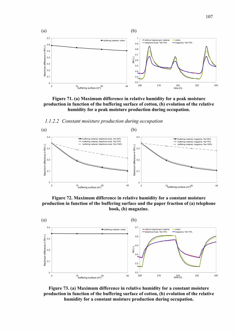
107

(a)

0

0.1

0.2

0.3

0.4

0.5

0.6

0.7

0 15 30 45

(b)

0.2

0.3

0.4

0.5

0.6

0.7

0.8

0.9

1

208 216 224 232 240time (h)

RH

(-)

without hygroscopic material


Max

imum

diff

eren

ce in

RH

(-)

cottonbuffering material: cottontelephone book, Ψp=75% magazine, Ψp=75%

Figure 71. (a) Maximum difference in relative humidity for a peak moisture production in function of the buffering surface of cotton, (b) evolution of the relative

humidity for a peak moisture production during occupation. 1.1.2.2 Constant moisture production during occupation

(a)

0

0.1

0.2

0.3

0.4

0 15 30 45

(b)

0

0.1

0.2

0.3

0.4

0 15 30 45buffering surface (m²)

Max

imum

diff

eren

ce in

RH

(-)


Max

imum

diff

eren

ce in

RH

(-)

buffering material: telephone book, Ψp=50% buffering material: magazine, Ψp=50%buffering material: telephone book, Ψp=75% buffering material: magazine, Ψp=75%buffering material: telephone book, Ψp=100% buffering material: magazine, Ψp=100%

Figure 72. Maximum difference in relative humidity for a constant moisture production in function of the buffering surface and the paper fraction of (a) telephone

book, (b) magazine.

(a)

0

0.1

0.2

0.3

0.4

0 15 30 45

(b)

0.2

0.3

0.4

0.5

0.6

0.7

208 216 224 232 240time (h)

RH

(-)

without hygroscopic material


Max

imum

diff

eren

ce in

RH

(-)

buffering material: cotton cottontelephone book, Ψp=75% magazine, Ψp=75%

Figure 73. (a) Maximum difference in relative humidity for a constant moisture production in function of the buffering surface of cotton, (b) evolution of the relative

humidity for a constant moisture production during occupation.

108

1.1.2.3 Concluding observations

We observe that for a moisture production with peaks, the cotton helps to decrease the

maximum difference in relative humidity (initially 59%) by 8% when having a

buffering surface of 45 m², this is a relative decrease of 14%. The cotton buffers a part

of the peak caused by the moisture production of 600 g/h. For the constant moisture

production this is not the case. This can be explained by the small thickness of the

cotton sheets (in our calculations 230µm). When there is a constant moisture production

for a longer period of time, the cotton sheets become fully loaded with moisture at the

ambient relative humidity and cannot buffer moisture anymore. As a consequence, its

influence on the relative humidity of the room is limited.

Looking at the books shows that a paper fraction of 75% gives quasi the same results as

a paper fraction of 50%; also there is almost no difference between the two types of

paper. When the books would be fully closed, a paper fraction of 100%, the difference

in hygroscopic capacity between telephone book paper and magazine paper becomes

clear. Books can decrease the maximum difference in relative humidity a lot more than

textiles, thanks to their larger volumes. For books, we have penetration depths for

moisture of centimeters, whereas the thickness of a textile fabric is only a hundred

micrometers. Books buffer moisture of peak moisture productions as well as of constant

moisture productions.

A book surface of 15m² with paper fractions for the books of 75% gives a relative

decrease of the maximum difference in relative humidity for the peak moisture

production of 48% for the telephone book, and 46% for the magazine. The decrease for

the constant moisture production is 43% for the telephone book and 41% for the

magazine.

1.1.3 Discussion

The simulations above illustrate that books can have an important influence on the

relative humidity fluctuations in a room, if the buffering surface is large enough. Thin

cotton sheets aid to buffer peaks in relative humidity. It can be expected that for thicker

textile materials (e.g. a carpet, curtains), this buffering effect will be more explicit.

The calculations in ROOMHAM do not take the hysteresis behaviour of cotton and

paper in account. Future work could include implementing the hysteresis effect in the

simulations.

109

To understand the effect of books and textiles on macro-scale thoroughly, a test room

should be build. In this way, theory and measurements could be compared and adjusted

to each other. The influence of the distance of the moisture source and the air movement

around books could be measured. In this way we would get an answer to the question

which surfaces of the books are accessible (only the top or also the back surface) and if

we can speak of a micro-climate around the books. The micro-climate would determine

then the buffering behaviour of the books. For example, it could be that the air reaches

the back side of a book later than the top surface when the book is standing on a book

rack. A first attempt for the design of a test room can be found in Appendix 6 (this

design still needs to be optimized!).

110

GENERAL CONCLUSION

This master thesis investigates first the hygroscopic properties of paper and textile. Two

paper materials were measured, a telephone book type of paper (this kind of paper is

also newspaper like) and a magazine type of paper. The macroscopic structure of these

materials is mainly build up by cellulose, and therefore, the hygroscopic mechanisms in

the materials are alike. The sorption curves and the vapour resistance factor were

measured in isothermal conditions. By this, the characteristic moisture properties, being

the moisture capacity and moisture permeability were determined. Both materials show

a hysteresis behaviour, the main adsorption isotherms lie below the main desorption

isotherms. This hysteresis behaviour is important in calculations, as the adsorption or

desorption path that is followed by the paper or the cotton influences the hygroscopic

buffering behaviour and therefore the results of calculations.

A model was developed to simulate the hygroscopic behaviour of books. Instead of

modelling a book by a two-material model, parallel layers of air and paper, a book is

homogenised, consisting of one ‘effective’ material. This model is based on two

characteristic features:

1. The air has a much lower moisture capacity than the paper, and therefore this

capacity can be neglected.

2. A book is a parallel system of air and paper, by which the vapour permeability is

determined by a summation of the vapour permeabilities of the paper and the air

layers, weighted with their respective fraction values.

With this model, it becomes easier to simulate the hygroscopic behaviour of books in

programs, as only a one dimensional model (1 material) needs to be used anymore,

instead of the previous two dimensional model (2 materials, air and paper).

It is shown that the air layers in between the paper sheets determine the rate of the

moisture uptake. As the air layer fraction in a book increases, the moisture uptake goes

faster and the book will reach equilibrium earlier than a fully closed book. The

hygroscopic loading of a book takes several weeks, as was also experimentally shown.

Book samples of five centimetre thickness were placed in a test setup going from 54 to

79,5% RH; after a period of 4 weeks, equilibrium was not yet fully attained.

111

For the measured cotton fabric, a finite element model was developed of the real fabric

structure. This model is more complex as the fabric has a three dimensional structure.

Also some simplifications must be made to develop the model, as there is a lot of

variation of the width of the cotton yarns and the dimensions of the holes in between the

yarns. The model can be used to understand the mechanism of moisture penetration in a

textile sheet. It is shown that the air holes in between the cotton yarns are determining

for the fast moisture uptake of a textile fabric. In isothermal conditions, textile fabrics

are loaded in a period of minutes.

Finally the measured properties and the developed effective book model were used in a

simulation program (ROOMHAM) to understand the effect of the materials on the

relative humidity fluctuations in a room. The simulations show that cotton can only

affect peaks in moisture production. Constant moisture productions will only be

buffered to a small amount by textile fabrics, as they attain their equilibrium with the

environment already after a few minutes. Books can buffer peaks in moisture

production as well as constant moisture productions significantly. Therefore the

available buffering surface must be large enough. This will be the case in for example

offices and libraries.

112

FUTURE WORK

Future work could consist of investigating which analytical description of the sorption

curves is the most appropriate for materials like paper and textile fabrics. In the

performed work, we used a description of the van Genuchten type, given by equation 6.

This description does not always give the best results, as could be seen through this

thesis report. The problem with equation 6 is that the parameter a should increase

(become closer to zero) to get better fits. But when doing this, the overall course of the

sorption curve is not correct anymore, as the capacity would decrease then at high

relative humidities, which contradicts reality.

At the end of the research, it was found that a description with the Mualem model could

be better. It would be interesting to investigate also other analytical descriptions, to find

the best description and implementing it in modelling programs.

The test with the book samples to determine the dynamic behaviour of books should be

repeated. Thinner books should be made (not with a thickness of five centimetres

anymore, but a lower thickness) so that the samples attain equilibrium faster. Also there

should be taken care of to ensure that the books follow the main adsorption curve.

Therefore the books should be fully dried first, then placed in an environment of

54%RH until they attain equilibrium and only then the dynamic loading can start. In this

way, the simulations of the test will become much more accurate. Also the influence of

determining the vapour permeability out of the cup test by equation 43 instead of 41

could be investigated.

The vapour permeability of the cotton fabric should be remeasured in a stationary way

instead of the dynamic loading test performed during the research. This dynamic

loading gave problems as the vapour resistance factor was found to be higher at 70%RH

than at 33%RH, which is impossible.

The calculations were done for steps in relative humidity. Future work could be to

simulate the effect of cyclic changes in relative humidity on books and textiles.

113

The calculations were all done assuming a constant temperature, so in isothermal

conditions. Future work could consist of calculating the coupled effect of heat and

moisture changes.

The hysteresis behaviour was not implemented in the ROOMHAM program when

calculating the effect of books and cotton on the relative humidity fluctuations. As the

hysteresis effect influences the hygroscopic behaviour of books and textiles, this could

be implemented in the future.

Also measurements should be done in a test room to combine theory and practice and

get an idea of what really happens in a room when buffering materials like books and

textiles are placed in it.

114

List of figures

Figure 1. Structure of cellulose. (Wikipedia).......................................................................... 11 Figure 2. Adsorption isotherms of paper (kg/kg)................................................................... 20 Figure 3. Adsorption isotherms of paper (kg/m³)................................................................... 20 Figure 4. Moisture capacity of paper (kg/kg). ........................................................................ 21 Figure 5. Moisture capacity of paper (kg/m³)......................................................................... 21 Figure 6. Vapour resistance factor of paper........................................................................... 22 Figure 7 (a)-(b): SEM images of the edge of telephone book paper. .................................... 25 Figure 8 (a)-(b) : SEM images of flat surface of telephone book paper. .............................. 26 Figure 9 (a)-(b): SEM images of the edge of magazine paper............................................... 26 Figure 10 (a)-(b): SEM images of flat surface of magazine paper........................................ 26 Figure 11. Picture of a dessicator. ........................................................................................... 29 Figure 12. (a): Full adsorption curve and desorption scanning curves for telephone book;

(b): Full adsorption curve and desorption scanning curves for magazine. Coloured

curves: analytical fit on main adsorption curve. ........................................................... 30 Figure 13. Mualem model-Measured (squares and bullets) and fitted (solid line) sorption

curves for (a) telephone book, (b) magazine. ................................................................. 32 Figure 14. Telephone book specimen in a cup to determine the vapour permeability. ...... 33 Figure 15. Results of the cup test to determine the vapour permeability for telephone book

and magazine. ................................................................................................................... 34 Figure 16. Measured data (squares) with standard deviation and fitted (solid line) curves

of the vapour resistance factor for (a) telephone book, (b) magazine. ........................ 36 Figure 17. Schematic overview of the test set-up used in the dynamic experiments........... 39 Figure 18. Samples for testing dynamic behaviour of books, (a) magazine paper, high and

low paper fraction; (b) telephone book paper, low paper fraction. ............................. 39 Figure 19. Book samples after dismantling of plexiglass, (a) telephone book high paper

fraction, (b) telephone book low paper fraction, (c) magazine low paper fraction. ... 39 Figure 20. (a) Evolution of the average moisture content (kg/kg) for the magazine and

telephone book (high paper fraction), (b) evolution of the difference in average

moisture content (kg/m³) for the magazine and telephone book (high paper fraction).

............................................................................................................................................ 42 Figure 21. (a) Evolution of the average moisture content (kg/kg) for high and low paper

fraction (magazine), (b) evolution of the difference in average moisture content

(kg/m³) for high and low paper fraction (magazine). .................................................... 43 Figure 22. REV (representative elementary volume) of a book............................................ 46

115

Figure 23. Schematic representation of 900 elements model, 420 and 200 elements model.

............................................................................................................................................ 47 Figure 24. Moisture content in (a) 900 elements model, (b) 420 and 200 elements model. 48 Figure 25. Moisture penetration profile in a paper sheet of 15 cm length; (a): influence of

air layer of same thickness as paper sheet -(b) no influence of air layer..................... 48 Figure 26. (a) Influence of surface coefficient and (b) air layer thickness when modelling

the hygroscopic behaviour of books................................................................................ 49 Figure 27. REV (representative elementary volume) of an effective book. ......................... 50 Figure 28. Real and effective phonebook simulation, Ψp 60%............................................. 52 Figure 29. Relation between correction factor mdelta and paper fraction Ψp. Diamonds:

simulation results. Line: linear approximation. ............................................................ 52 Figure 30. Moisture transport mechanisms in a book. .......................................................... 54 Figure 31. Correction factor meffus for the telephone book and magazine paper. ............... 56 Figure 32. Effusivity of telephone book and magazine paper. .............................................. 56 Figure 33. Real and effective phonebook simulation, Ψp 60%, vapour permeability paper

is variable. ......................................................................................................................... 57 Figure 34. Mass of the specimens in the dynamic test of books, measurements (solid lines)

and analytical description (dashed lines) for (a)-(b) telephone book, (c)-(d) magazine.

............................................................................................................................................ 59 Figure 35. Measured weight change of telephone book sample with low paper fraction,

when imposing a step in RH from 54 to 79,5% RH (at test setup TU Eindhoven). ... 60 Figure 36. Comparison between correction factor for vapour permeability of book model

(assuming main adsorption) and analytical description; (a) telephone book, (b)

magazine............................................................................................................................ 62 Figure 37. Vapour resistance factor of telephone book in function of (a) saturation degree;

(b) relative humidity for main adsorption and main desorption. ................................ 64 Figure 38. Vapour resistance factor of magazine in function of (a) saturation degree; (b)

relative humidity for main adsorption and main desorption. ...................................... 65 Figure 39. Moisture content of magazine book samples........................................................ 66 Figure 40. Moisture capacity and vapour resistance factor of magazine book sample with

high paper fraction........................................................................................................... 66 Figure 41. Simulating the dynamic behaviour of magazine high paper fraction, with

effective book model......................................................................................................... 67 Figure 42. Moisture capacity and vapour resistance factor of magazine book sample with

low paper fraction. ........................................................................................................... 68 Figure 43. Simulating the dynamic behaviour of magazine low paper fraction, with

effective book model......................................................................................................... 68

116

Figure 44. Moisture content of telephone book samples. ...................................................... 69 Figure 45. Moisture capacity and vapour resistance factor of telephone book sample with

high paper fraction........................................................................................................... 70 Figure 46. Simulating the dynamic behaviour of telephone book high paper fraction, with

effective book model......................................................................................................... 71 Figure 47. Moisture capacity and vapour resistance factor of telephone book sample with

low paper fraction. ........................................................................................................... 71 Figure 48. Simulating the dynamic behaviour of telephone book low paper fraction, with

effective book model......................................................................................................... 72 Figure 49. Comparison between vapour resistance factors using equation 41 or 43, for (a)

telephone book, (b) magazine. ......................................................................................... 75 Figure 50. Schematics of woven composites. (Tang et al, 2005)............................................ 77 Figure 51. Adsorption isotherms of textiles (g/g); dots=data from literature, continuous

lines=fitted curves............................................................................................................. 85 Figure 52. Adsorption isotherms of textiles (kg/m³)............................................................... 85 Figure 53. Moisture capacity of textiles (g/g).......................................................................... 86 Figure 54. Moisture capacity of textiles (kg/m³)..................................................................... 86 Figure 55. Vapour resistance factor of textiles. ...................................................................... 87 Figure 56 (a)-(b): Microscope images of flat surface of cotton; (c)-(d): SEM images of flat

surface of cotton. .............................................................................................................. 89 Figure 57 (a)-(b): Microscope images of fibers of cotton; (c)-(d): SEM images of fibers of

cotton. ................................................................................................................................ 90 Figure 58 (a)-(b): SEM images of the edge of cotton. ............................................................ 90 Figure 59. Graphical output of Quips program; (a): areas between cotton yarns, (b)

distances of cotton fabric. ................................................................................................ 91 Figure 60. Area between cotton yarns of (a) x40 enlargement and (b) x80 enlargement;

distance between cotton yarns (calculated as ‘equivalent side’ of areas) of (c) x40

enlargement and (d) x80 enlargement. ........................................................................... 92 Figure 61. Distance between cotton yarns of (a) x40 enlargement and (b) x80 enlargement;

width of cotton yarn of (a) x40 enlargement and (b) x80 enlargement. ...................... 93 Figure 62. Full adsorption curve and desorption scanning curves for cotton. Coloured

curve: analytical fit on main adsorption curve.............................................................. 94 Figure 63. Mualem model-Measured (squares and bullets) and fitted (solid line) sorption

curves for cotton fabric.................................................................................................... 95 Figure 64. Cotton sample for dynamic vapour permeability test. ........................................ 96 Figure 65. Test setup for determining vapour permeability of cotton by dynamic test. .... 96 Figure 66. REV of a cotton fabric............................................................................................ 98

117

Figure 67. REV of textile sheet in GID (modelling program). .............................................. 99 Figure 68. Real and effective textile simulation.................................................................... 100 Figure 69. (a) Moisture content and (b) RH difference between nodes of cotton yarns, real

textile model. ................................................................................................................... 101 Figure 70. Maximum difference in relative humidity for a peak moisture production in

function of the buffering surface and the paper fraction of (a) telephone book, (b)

magazine.......................................................................................................................... 106 Figure 71. (a) Maximum difference in relative humidity for a peak moisture production in

function of the buffering surface of cotton, (b) evolution of the relative humidity for a

peak moisture production during occupation.............................................................. 107 Figure 72. Maximum difference in relative humidity for a constant moisture production in

function of the buffering surface and the paper fraction of (a) telephone book, (b)

magazine.......................................................................................................................... 107 Figure 73. (a) Maximum difference in relative humidity for a constant moisture

production in function of the buffering surface of cotton, (b) evolution of the relative

humidity for a constant moisture production during occupation.............................. 107

118

List of tables

Table 1. Material characteristics of paper.............................................................................. 18 Table 2. The parameters for the analytical fit of the adsorption isotherms for different

types of paper.................................................................................................................... 19 Table 3. The parameters for the analytical fit of the resistance factor for paper. .............. 22 Table 4. Chemical composition of telephone book and magazine. ....................................... 27 Table 5. The parameters for the analytical fit of the adsorption isotherms for telephone

book and magazine........................................................................................................... 29 Table 6. The parameters for the Mualem model of the sorption isotherms for telephone

book and magazine........................................................................................................... 31 Table 7. Water vapour resistance factors for telephone book and magazine...................... 35 Table 8. Parameters for the fit of the vapour resistance factor for telephone book and

magazine............................................................................................................................ 35 Table 9. Dimensions of book specimens for dynamic testing. ............................................... 38 Table 10. Data of the test specimens for dynamic testing...................................................... 38 Table 11. Dimensions of the calcium silicate specimens used in TU Eindhoven test setup to

determine surface mass transfer coefficient. ................................................................. 40 Table 12. Parameters for the analytical description of the dynamic behaviour of books

(adsorption)....................................................................................................................... 59 Table 13. Estimation of book capacity and vapour permeability for tested book samples,

based on the book model, assuming that books follow main adsorption curve. ......... 61 Table 14. Comparison between expected moisture content of book samples and measured

moisture content. .............................................................................................................. 63 Table 15. Moisture content of magazine book samples. ........................................................ 65 Table 16. Parameters for fit of sorption curve of magazine book samples.......................... 65 Table 17. Parameters for fit of sorption curve of telephone book samples.......................... 69 Table 18. Moisture content of telephone book samples. ........................................................ 69 Table 19. Parameters for the fit of the vapour resistance factor of telephone book and

magazine, applying equation 43. ..................................................................................... 73 Table 20. Typical values of fiber densities. (From 'Physical properties of textile fibers',

p.156). ................................................................................................................................ 78 Table 21. Material characteristics of textiles.......................................................................... 83 Table 22. The parameters for the analytical fit of the sorption isotherms for different types

of textiles. .......................................................................................................................... 84 Table 23. The parameters for the analytical fit of the resistance factor for textiles. .......... 87

119

Table 24. Mean values of distance between cotton yarns and width of cotton yarn from

Quips program. ................................................................................................................ 92 Table 25. Water vapour resistance factors for cotton fabric. ............................................... 96 Table 26. Moisture production in room. ............................................................................... 104 Table 27. Density and heat properties of materials used in ROOMHAM modelling. ...... 105 Table 28. Moisture parameters of materials used in ROOMHAM modelling. ................. 105

120

References

Carmeliet J., de Wit M., Janssen H., 2005. Hysteresis and moisture buffering of wood.

Symposium of Building Physics in the Nordic Countries, June 13-15 2005, Reykjavik,

Iceland, pp.55-62.

Chatterjee S.G., 2001. Comparison of Domain and Similarity Models for Characterizing

Moisture Sorption Equilibria of Paper. Industrial and Engineering Chemical Research,

Vol. 40, pp.188-194.

Efremov G.I., 2005. Calculations of the effective diffusion coefficient in drying of

polymers, fibres, and composite materials with a quasistationary method. Fibre

Chemistry, Vol. 37, No. 1, pp.67-72.

Foss W.R., Bronkhorst C.A., Bennett K.A., 2003. Simultaneous heat and mass transport

in paper sheets during moisture sorption from humid air. International Journal of Heat

and Mass Transfer, Vol. 46, pp.2875-2886.

Ghali K., Ghaddar N., Jones B., 2002. Emperical Evaluation of Convective Heat and

Moisture Transport Coefficients in Porous Cotton Medium. Journal of Heat Transfer,

Vol. 124, pp.530-537.

Goossens E., 2003. Moisture transfer properties of coated gypsum. PhD-thesis TU/e,

Eindhoven, The Netherlands.

Gupta H., Chatterjee S.G., 2003. Parallel Diffusion of Moisture in Paper. Part 1: Steady-

State Conditions. Industrial and Engineering Chemical Research, Vol. 42, pp.6582-

6592.

Gupta H., Chatterjee S.G., 2003. Parallel Diffusion of Moisture in Paper. Part 2:

Transient Conditions. Industrial and Engineering Chemical Research, Vol. 42,

pp.6593-6600.

121

Hagentoft C.E. et al, 2004. Assessment Method of Numerical Prediction Models for

Combined Heat, Air and Moisture Transfer in Building Components: Benchmarks for

One-dimensional Cases. Journal of Thermal Envelope and Building Science, Vol. 27,

No. 4, pp.327-351.

Hens H., 2003. Bouwfysica 1, Warmte- en massatransport. Uitgeverij Acco, zesde,

gewijzigde druk 2003.

Hens H., 2003. Toegepaste bouwfysica 1, Randvoorwaarden, prestaties,

materiaaleigenschappen. Uitgeverij Acco, derde, volledig herwerkte uitgave 2003.

Janssen H., Blocken B., Carmeliet J., 2005. Conservative modelling of the moisture and

heat transfer in building components under atmospheric excitation. Accepted for

International Journal for Heat and Mass Transfer.

Kumaran, K., 1996. International Energy Agency, Condensation and energy –

Catalogue of material properties. Report Annex XIV Volume 3, Energy conservation in

buildings.

Leisen J., Beckham H.W., Benham M., 2003. Sorption Isotherm Measurements by

NMR. Solid State Nuclear Magnetic Resonance, Vol. 22, pp.409-422.

Morton W.E., Hearle J.W.S., 1993. Physical properties of Textile Fibres. Published by

the Textile Institute, third edition 1993.

Niskanen, K., 1998. Papermaking Science and Technology Book 16: Paper Physics.

The Finnish Pulp and Paper Research Institute.

Okubayashi S., Griesser U.J., Bechtold T., 2004. A kinetic study of moisture sorption

and desorption on lyocell fibers. Carbohydrate Polymers, Vol. 58, pp.293-299.

Motta Lima O.C., Monteiro A.S., Pereira N.C., Mendes E.S., 2003. Moisture

Equilibrium Isotherms for a Commercial Liquid Package Paper. Drying Technology,

Vol. 21, No. 10, pp.1909-1922.

122

Ramarao B.V., Massoquete A., Lavrykov S., Ramaswamy S., 2003. Moisture Diffusion

Inside Paper Materials in the Hygroscopic Range and Characteristics of Diffusivity

Parameters. Drying Technology, Vol. 21, No. 10, pp.2007-2056.

Ramaswamy S., Gupta M., Goel A., Aaltosalmi U., Kataja M., Koponen A., Ramarao

B.V., 2004. The 3D structure of fabric and its relationship to liquid and vapor transport.

Colloids and Surfaces A: Psychochemical and Engineering Aspects, Vol. 241, pp.323-

333.

Roels S., 2004. Inter-laboratory comparison on measurement of moisture buffering

properties of gypsum board. Instruction document to Annex 41 Moist-Eng Subtask 2:

Experimental analysis of Moisture Buffering.

Roels S., Carmeliet J., 2005. Water vapour permeability and sorption isotherm of coated

gypsum board. Proceedings of the 7th symposium on Building Physics in the Nordic

Countries, The Icelandic Building Research Institute, Reykjavik, Iceland.

Roels S., Janssen H., 2005. Is the moisture buffer value a reliable material property to

characterise the hygric buffering capacities of building materials? Working document to

IEA Annex 41 Moist-Eng 4th working meeting, October 26-28 2005, Trondheim,

Norway.

Schick M.J., 1975. Surface characteristics of fibers and textiles.

Shirmer R., 1938. Die Diffusionszahl von Wasserdampf-Luftgemischen und die

Verdampfungs-geschwindigkeit. VDI Beheift Verfahrenstechnik, nr. 6, 170.

Svennberg K., 2003. Determination of Moisture Properties for Materials Exposed to the

Indoor Air. Licentiate thesis, Lund University, Sweden.

Svennberg K., 2004. Sorption isotherms for textile fabrics and foam used in the indoor

environment. Working document to IEA Annex 41 Moist-Eng 2nd working meeting,

October 27-29 2004, Glasgow, UK.

123

Svennberg K., 2004. Determination of moisture properties and verification of step-

responses for materials and material combinations. Working document to IEA Annex

41 Moist-Eng Subtask II meeting, May 12-14 2004, Zürich, Switzerland.

Svennberg K., Hedegaard L., Rode C., 2004. Moisture Buffer Performance of a Fully

Furnished Room. Proceedings of Performance of Exterior Envelopes of Whole

Buildings IX, International Conference, December 5-10 2004, US Department of

Energy, Oak Ridge National Laboratory, 2004 ASHRAE.

Svennberg K., Claesson J., Hansen K., 2005. Moisture penetration in a chair seat as a

response to daily RH variations in the indoor air. Proceedings of the 7th symposium on

Building Physics in the Nordic Countries, The Icelandic Building Research Institute,

Reykjavik, Iceland, pp.703-710.

Tang X., Whitcomb J.D., Yanmei L., Sue H., 2005. Micromechanics modelling of

moisture diffusion in woven composites. Composites Science and Technology, Vol. 65,

pp.817-826.

Zhu Q., Li Y., 2003. Effects of pore size distribution and fiber diameter on the coupled

heat and liquid moisture transfer in porous textiles. International Journal of Heat and

Mass Transfer, Vol. 46, pp.5099-5111.

Standards

EN ISO 12572, June 2001. Hygrothermal performance of building materials and

products – Determination of water vapour transmission properties.

Brochures

Philips, 1996. Environmental Scanning Electron Microscopy.

JEOL. Invitation to the SEM World, for people who are using the SEM for the first

time.

124

Websites

www.paperonweb.com

w3.upm-kymmene.com

www.isobar.be

www.dantecdynamics.com

www.wikipedia.org

role of textiles and paper for stabilizing the … · we take the influence of the indoor materials...

Documents