roughness coefficient of a highly calcinated penstock

Teknik Dergi, 2019 9309-9325, Paper 545

Roughness Coefficient of a Highly Calcinated Penstock* Kutay ÇELEBIOĞLU1 ABSTRACT

When highly calcinated water is transferred through the penstock of a hydropower plant it leaves a residue on the pipe surface. Accumulated residue over time causes a change in the roughness of the pipe surface thus leads to friction losses in the system. The effect is a change in head and discharge relation for the turbines. A multimethodology is proposed for determining the apparent surface roughness value (ε) by means of friction factor f and measuring arithmetic mean deviation of the roughness profile (Ra), root mean square roughness (Rq) and peak and valley roughness (Rz). It is found that a surface roughness value (ε) of 0.3mm can be used for calcinated surfaces which is much higher than steel surfaces but smaller than a concrete surface.

Keywords: Friction factor, surface roughness, calcination.

1. INTRODUCTION

Energy output of hydropower plants (HPP) depends on the net head and flow rate supplied to the turbines. Water is conveyed from a reservoir or a head pond to the power house by means of water conduits called penstocks. Systems are designed such that the energy output is maximized while minimizing the cost [1]. Part of the available energy is lost due to pipe friction and other local losses. Available energy conveyed to the turbines, hence the amount of energy produced, depends on the amount left after these losses.

When highly calcinated water is transferred through the penstock of a hydropower plant it leaves a residue on the pipe surface. Such residues accumulate over time forming a thick layer on the surfaces in contact with water. There are two important aspects of this calcination, one is the change in the surface roughness coefficient the other is the change in the actual flow diameter. While the effect of the first one is not known a priori, the second one causes a decrease in flow diameter and an increase in the average velocity, increasing losses in the penstock system.

Note:

- This paper has been received on July 24, 2018 and accepted for publication by the Editorial Board on November 23, 2018.

- Discussions on this paper will be accepted by September 30, 2019. https://dx.doi.org/10.18400/tekderg.447265 1 TOBB University of Economics and Technology, Hydro Energy Research Center, Ankara, Turkey -

[email protected] - https://orcid.org/0000-0001-8845-4928

Roughness Coefficient of a Highly Calcinated Penstock

9310

Recently, a rehabilitation project for and old powerhouse (KEPEZ 1 HPP), located in the province of Antalya, was started. The Hydropower plant is equipped with three Francis type turbines with an installed capacity of 26.4 MW. It is the sixth largest power house in the region. The power house had been in operation for more than 30 years. The net head of the turbines is 162 m with a discharge of 6.1 m3/s. The aim of the rehabilitation project is to increase efficiency and output of the old turbines in the HPP by replacing them with new ones while renewing all auxiliary systems up to state-of-the-art requirements.

The hydro power plant consists of a head pond and an intake structure and diverts the flow through a pressurized concrete pipe followed by a surge tank and a long steel pipe. A problem concerning quality of water exists in the region, causing heavy calcination of pipes. Operating records of the power house suggests a calcination period that is as short as six months and a calcination thicknesses of up to 30 mm were observed in the penstock. Continuous cleaning of the water conduit is very costly and interrupts energy production because it requires emptying the penstock and hard scrubbing of the full conduit system. Thus, a new turbine to be installed on the old calcinated pipeline system will operate at different head than its design head and at different discharge conditions than its initial design. Therefore, the new turbine design should account for calcination and change in the friction losses in the system for varying flowrates.

Initial design net head and discharge through the turbines are determined using the design drawings. They are calculated from the well-established Darcy-Weisbach relation. When designing a new system, the equivalent roughness values of steel (ε=0.02 - 0.05mm) and concrete pipes (ε=0.5mm) are easily obtained from various engineering tables and the net head available to the turbine can easily be calculated [2]. Roughness coefficients of selected residue materials are also available in the literature [3]. But no information is available in literature for the apparent surface roughness value (ε) of a highly calcinated pipe surface. For this reason, a multimethodology is proposed that includes:

1.) A one-dimensional numerical model of the existing system which is built to calculate the steady state head and discharge relation for varying apparent surface roughness values (ε)

2.) Determination of combined friction coefficient based on site measurements of flow rate and turbine inlet pressure and head water level variations

3.) Determination of apparent surface roughness using laboratory measurements of surface profile and waviness of a sample calcinated block obtained from the site.

The numerical model is used to observe the variation in the combined friction coefficient of the system by changing the surface roughness values (ε) of individual pipes. Then, site measurements are used to calculate the friction coefficient of the system. This coefficient is compared with the surface roughness values (ε) of the numerical model to estimate how a calcinated pipe surface behaves for the heavily calcinated penstock so that the turbine operating range can be determined. Lastly, during the dismantling of the old turbines, the penstock is emptied and became accessible to receive samples from the penstock surface. Surface roughness of the sample is measured in the laboratory to confirm the friction slopes, apparent surface roughness values (ε), and measured roughness profiles that point to the same result.

Kutay ÇELEBİOĞLU

9311

2. NUMERICAL MODEL

A convenient form of the Energy Equation for a steady, incompressible flow with uniformly distributed velocity profiles can be written between the two sections in a straight pipe as:

+ + 𝑍 = + + 𝑍 + 𝐻 (1)

where, P is the pressure, V is the average velocity, Z is the elevation of the pipe axis, ρ is the density of the fluid, g is the gravitational acceleration, and HL is the frictional head loss between these two sections, given that there are no minor losses. In 1845, Julius Weisbach [4] proposed an equation that predicts the losses due to fluid friction on the pipe wall as; 𝐻 = 𝑓 (2)

𝑓 = 𝑓𝑢𝑛𝑐 , 𝑅𝑒 (3)

where L is the pipe length, D is the pipe diameter, f is a friction factor, Re is the Reynolds number and is defined by Re=VD/ν and ν is the kinematic viscosity of the fluid. This equation set the standard for all following engineering text books [2]. With Darcy’s estimates of the friction factor [5] and additional work by Colebrook and White [6] on non-uniform roughness, estimates of the friction factor f can be made as functions of Reynold number (Re) and relative roughness (ε/D). Later Moody [7] published the famous Moody’s chart and Swamee and Jain [8] expanded the form to the explicit equations for pipe diameter, head loss and the discharge through a pipe, based on the Colebrook-White equation [6].

For long penstock systems, friction in each pipe segment can be calculated separately. Pipe diameters, lengths and corresponding Reynolds numbers are different in each pipe segment. Minor losses due to bends, expansions, contractions etc. can be calculated separately as a function of discharge and all of these losses can be added to obtain the system loss. In order to generalize the equation of losses, the Darcy-Weisbach equation can be written such that the head loss due to friction becomes a function of discharge: 𝐻 = (8𝑓𝐿 𝑔𝜋 𝐷⁄ )𝑄 = 𝑘 𝑄 (4)

Minor (local) losses such as those due to bends, expansions contractions etc. can also be formulated as a function of discharge; 𝐻 = 𝑘 𝑄 (5)

Then the total loss in the system can be calculated by adding all friction and local losses. 𝐻 = ∑ 𝑘 𝑄 + ∑ 𝑘 𝑄 = 𝑘 𝑄 + 𝑘 𝑄 = 𝑘𝑄 (6)

Where k is a combined friction coefficient for the entire system. A numerical one-dimensional model is designed for the existing system as shown in Figure 1, where the head


9312

pond is modeled as reservoir 1 (R1). Water is conveyed through a concrete pipe (E1) and a series of steel pipes (P1-P9, B1, S1) to turbine and then to the Tailrace Channel (T1). The model is set up with one turbine in operation in order to compare the results with the measurements.

Figure 1 - Layout of the Kepez 1 HPP

Basic parameters including minor loss coefficients of the pipe system are given in Table 1.

Table 1 - System parameters

Label Material Diameter (cm) Minor Loss Coefficient Length (m) P2 Steel 240 0.040 62.16 P4 Steel 240 0.000 164.60 P6 Steel 210 0.110 103.87 P3 Steel 240 0.006 44.33 P5 Steel 240 0.000 100.50 P1 Steel 240 0.062 23.01 T1 Concrete 500 0.000 5.00 P7 Steel 210 0.019 206.66 P8 Steel 210 0.060 62.88 E1 Concrete 250 0.346 589.00 B1 Steel 130 0.052 1.00 S1 Steel 90 0.169 3.60 P9 Steel 210 0.096 19.97

The head pond and tailrace levels are set to constant values for each simulation and the corresponding friction and minor losses are calculated. The discharge passing through the system is controlled by the guide vanes of the Francis turbine. The model is set such that the simulated discharge range covers the operation of the installed Francis turbine. A head discharge curve is used for each guide vane opening for the Francis Turbine. A total of 12 simulations are performed for three discharge sets (Table 2) and four roughness values (Table 3). Simulations are iterated until the discharge values are seen to converge with the preset values.

Kutay ÇELEBİOĞLU

9313

Table 2 - Simulated flowrates

Q1

(m3/s) Q2

(m3/s) Q3

(m3/s) Case 3.0344 5.3758 6.1471

Table 3 - Apparent surface roughness values

ε1 (mm) ε2 (mm) ε3 (mm) ε4 (mm) Case 0.5 0.3 0.05 0.02

There are various engineering tables that present the apparent roughness values (ε) of different materials [2]. The values of interest in this study are for smooth and rough steel pipes (0.02 mm and 0.05 mm) and concrete (0.3~3 mm). A representative value of 0.5 mm is selected for smooth concrete. A comparative study is performed to observe how the roughness of calcinated surface changes with respect to steel and concrete. So, simulated values for the calcinated pipes included these values in addition to an intermediate value of 0.3mm. Since calcination occurs both in concrete and steel surfaces, roughness values are kept constant for all simulations throughout the system. During measurements, sensor taps were drilled on the steel pipe to install acoustic flow meters. The drilled hole and calcinated layer are shown in Figure 2. The thickness of the calcinated layers can be seen through these holes and found to vary between 11 mm and 15 mm. Although the effect of change in the flow diameter due to this accumulation is small, it is considered in all of the simulations and all pipe diameters presented in Table 1 is reduced by 30mm.

Figure 2 - Calcination in the pipe seen from a sensor tap

Friction and minor losses are calculated for each pipe segment and tabulated for each simulation. These values are summed up to calculate the total loss in each simulation. A sample computation for the flow rate of 6.147 m3/s, head pond elevation of 278.2 m, tailwater elevation of 110.04 m and an apparent roughness values (ε) of 0.3 mm is given in Table 4.


9314

Table 4 - Solution values for a case

Label Material Velocity (m/s)

Headloss (m)

Headloss (Friction) (m)

Headloss (Minor) (m)

P2 Steel 1.39 0.038 0.034 0.004 P4 Steel 1.39 0.090 0.090 0.000 P6 Steel 1.77 0.123 0.105 0.018 P3 Steel 1.39 0.025 0.024 0.001 P5 Steel 1.39 0.055 0.055 0.000 P1 Steel 1.39 0.019 0.013 0.006 T1 Concrete 0.31 0.000 0.000 0.000 P7 Steel 1.77 0.213 0.210 0.003 P8 Steel 1.77 0.073 0.064 0.010 E1 Concrete 1.28 0.289 0.260 0.029 B1 Steel 4.85 0.076 0.014 0.063 S1 Steel 9.77 1.122 0.301 0.821 P9 Steel 1.77 0.036 0.020 0.015

Sum 2.157 1.188 0.969

In order to calculate the combined system friction constant k for each apparent roughness value (ε), total head loss in each simulation is calculated and tabulated against flowrate and square of the flowrate. Results of all simulations are summarized in Table 5.

Table 5 - Head loss values in meters for 12 cases

ε1 (mm) ε2 (mm) ε3 (mm) ε4 (mm)

Q (m3/s) 0.5 0.3 0.05 0.02 6.1471 2.275 2.157 1.898 1.835 5.3758 1.742 1.653 1.459 1.413 3.0344 0.559 0.532 0.477 0.465

As the head loss changes linearly with Q2 value according to Darcy-Weisbach equation, results are plotted and a line is fitted to obtain friction head loss slope coefficient as shown in Figure 3. Coefficient values of 0.0488, 0.0504, 0.0572 and 0.0603 are obtained for roughness values of 0.02 mm, 0.05mm, 0.3mm and 0.5mm respectively.

Kutay ÇELEBİOĞLU

9315

Figure 3 - Calculation of friction head loss slope for different roughness coefficients

3. CALCULATION OF FRICTION COEFFICIENT BASED ON SITE MEASUREMENT

Kepez HPP has been in operation for more than 30 years. During this period significant improvement in turbine design was achieved with the help of computational fluid dynamics (CFD)[9]. Efficiency and cavitation characteristics of runner is investigated and characteristics over operating region of the old Kepez turbine is determined by means of CFD [10][12]. Design of the new turbine is significantly improved to better characterize the current operating regime [13]. The new turbine efficiency is obtained by means of both CFD [13] and model tests [14] performed at ETU HYDRO Turbine Design and Test Center. Although these works give significant insight on the turbine performance, project requirements dictate comparison of efficiencies with in-situ site measurements. For this reason, an efficiency measurement setup is installed at site as part of the project[15]. Using this setup, hydraulic efficiency of the turbine is measured at different operating points [15]. Available hydraulic energy to the turbine and power output of the generator are required to calculate efficiency of the turbine generator set. To obtain the available hydraulic energy, the turbine net head and flowrate must be known. Pressure measurement taps are installed for measuring the inlet and outlet pressures before and after the turbine. An ultrasonic flow measurement system is installed for measuring the flow rate. For efficiency calculations, the mechanical power out of the turbine must also be determined. Power output of the generator can be measured through the current and voltage transformers. Energy analyzers were installed at outputs of generator current and voltage transformers to obtain the electrical output of the generator. With known generator efficiency curve and output of the generator, shaft power can be


9316

calculated. So, hydraulic efficiency of the turbine can be calculated from available hydraulic energy and mechanical power. Using this methodology efficiency of the old turbine is measured [15]. Via these pressure taps and ultrasonic flow meters, the pressure at the turbine inlet as well as the discharge passing through the system is readily available and given in Table 6.

Table 6 - Flowrate, Pressure and Change in Head pond levels

Q [m³/s] P (kPa) ΔHHPL (m) 6.1471 1619.67 0.65 6.0696 1619.90 0.77 5.7974 1622.51 0.77 5.6236 1626.25 0.20 5.5628 1626.44 0.69 5.3758 1627.50 0.77 5.1572 1629.19 0.12 4.8804 1630.61 0.00 4.2254 1636.40 0.65 3.0344 1642.69 0.74

Table 7 - System curve calculations

Q [m³/s] V2/2g (m) P/γ (m) Hinlet (m)

Hinlet -ΔHHPL (m)

6.1471 1.094 165.296 166.390 165.740 6.0696 1.067 165.319 166.386 165.616 5.7974 0.973 165.586 166.559 165.789 5.6236 0.916 165.967 166.883 166.683 5.5628 0.896 165.986 166.883 166.193 5.3758 0.837 166.095 166.932 166.162 5.1572 0.770 166.267 167.037 166.917 4.8804 0.690 166.412 167.101 167.101 4.2254 0.517 167.003 167.520 166.870 3.0344 0.267 167.645 167.911 167.171

This data set is used to calculate the head discharge relation of the system and the friction slope coefficient of the conduit. An additional data, head pond level, is required to calculate

Kutay ÇELEBİOĞLU

9317

a system curve. Since no digital measurement system for the head pond levels was available, hourly operating records of head pond level change with respect to crest elevation using a rod installed at the head pond is used. The change in the reservoir level is measured and tabulated below together with flowrate and pressure (Table 6).

System losses are calculated from the slope of the curve Hinlet -ΔHHPL vs Q2. The corresponding values are obtained by adding the velocity head, pressure head and subtracting the variation in the head pond level as given in Table 7.

Results are plotted for total head vs square of flowrate and a line is fitted to obtain friction slope coefficient from measurements as shown in Figure 4. As the head loss changes linearly with Q2 value according to Darcy-Weisbach equation, a line is fitted and slope is calculated as -0.0562 (Figure 4).

Figure 4 - Calculation of friction slope from measurements

The curve represents the change in the total head with increasing discharge, thus a negative value. Absolute value of this slope is 0.0562 which is compared with the various roughness values calculated and plotted via the numerical model, the surface roughness value (ε), 0.3mm shows a similar a slope of 0.0572.

4. LABORATORY MEASUREMENTS OF SURFACE ROUGHNESS

Once the design and manufacturing of the new turbine was completed, dismantling of the old turbine system was started. Energy production interrupted, the penstock was emptied. The old turbine system as well as the inlet valve was removed. At that stage, access to the penstock was available. A sample block of calcinated residue is carefully taken for testing purposes


9318

without disturbing the surface, size and thickness of the calcinated sample taken from the penstock are shown in Figure 5.

Figure 5 - Calcinated sample from penstock

Sides of the block are grinded and the block is attached to a clamp. A Zeiss Surfcom 130 A surface profiler is used to measure the surface profile of the block.

Figure 5 - Measurement of Surface profile

A sampling section is measured with a length of 38 mm. A probe with a tip radius of 2 μm, a speed of 0.6mm/s is used. The primary (total) profile, which is the surface height measured throughout the sampling section, is measured and shown in Figure 6. The waviness component is obtained from an electronic low-pass filtering of the primary profile with a cut off wavelength value of 8.0 mm (Figure 6). Finally, roughness profile is obtained (Figure 7). By doing so, the measured profile is filtered for large scale waviness effects and a representative data set for the surface characteristics that effect friction is obtained. This data set is necessary to calculate measurable surface roughness characteristics Ra, Rq and Rz.

Kutay ÇELEBİOĞLU

9319

Figure 6 - Total profile and waviness

Figure 7 - Roughness profile

Once the roughness profile is obtained, standard surface roughness parameters (Ra, Rq, Rz) are calculated using equations 7, 8 and 9. The first parameter Ra represents the arithmetical

-200

-150

-100

-50

0

50

100

150

0 200 400 600 800 1000 1200

Surfa

ce h

eigh

t in

μm

Length in μm

Surface Profile Measurements

Total Profile Filtered Waviness

-200

-150

-100

-50

0

50

100

150

0 200 400 600 800 1000

Surfa

ce h

eigh

t in

μm

Length in μm

Roughness Profile

Roughness Profile


9320

mean of the absolute values of the profile deviations from the mean line of the roughness and is given by: 𝑅𝑎 = |𝑧(𝑥)|𝑑𝑥 (7)

whereas the root mean square roughness Rq is given by:

𝑅𝑞 = 𝑧 (𝑥)𝑑𝑥 (8)

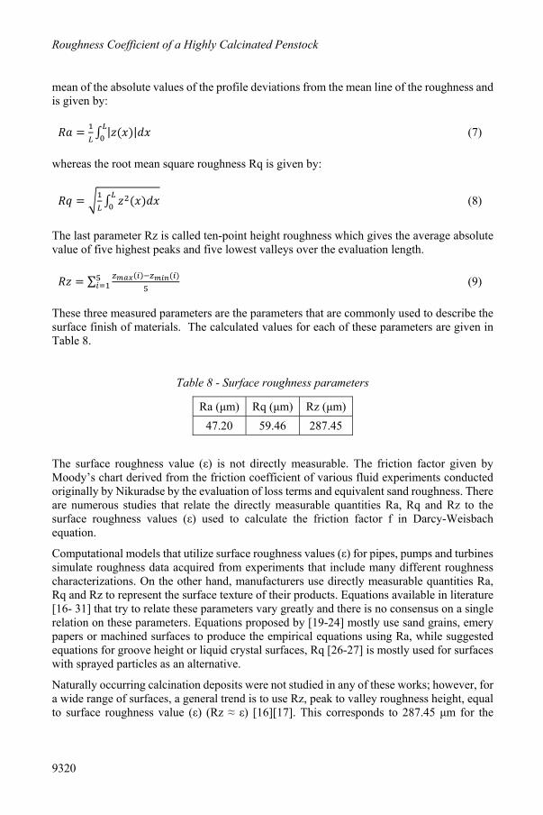
The last parameter Rz is called ten-point height roughness which gives the average absolute value of five highest peaks and five lowest valleys over the evaluation length. 𝑅𝑧 = ∑ ( ) ( ) (9)

These three measured parameters are the parameters that are commonly used to describe the surface finish of materials. The calculated values for each of these parameters are given in Table 8.

Table 8 - Surface roughness parameters

Ra (μm) Rq (μm) Rz (μm) 47.20 59.46 287.45

The surface roughness value (ε) is not directly measurable. The friction factor given by Moody’s chart derived from the friction coefficient of various fluid experiments conducted originally by Nikuradse by the evaluation of loss terms and equivalent sand roughness. There are numerous studies that relate the directly measurable quantities Ra, Rq and Rz to the surface roughness values (ε) used to calculate the friction factor f in Darcy-Weisbach equation.

Computational models that utilize surface roughness values (ε) for pipes, pumps and turbines simulate roughness data acquired from experiments that include many different roughness characterizations. On the other hand, manufacturers use directly measurable quantities Ra, Rq and Rz to represent the surface texture of their products. Equations available in literature [16- 31] that try to relate these parameters vary greatly and there is no consensus on a single relation on these parameters. Equations proposed by [19-24] mostly use sand grains, emery papers or machined surfaces to produce the empirical equations using Ra, while suggested equations for groove height or liquid crystal surfaces, Rq [26-27] is mostly used for surfaces with sprayed particles as an alternative.

Naturally occurring calcination deposits were not studied in any of these works; however, for a wide range of surfaces, a general trend is to use Rz, peak to valley roughness height, equal to surface roughness value (ε) (Rz ≈ ε) [16][17]. This corresponds to 287.45 μm for the

Kutay ÇELEBİOĞLU

9321

calcinated surface sample. Regardless, a table is prepared from available literature to calculate and check surface roughness values (ε) using all three parameters Ra, Rq, Rz. Values of surface roughness (ε) are calculated using these three parameters as given in Table 9 [16-31].

These values are averaged to find a single representative number for ε which is found to be 281.70 μm. The calculated average surface roughness (ε) value of 281.70 μm is also found to be very close to simulated 300 μm roughness value which corresponds to combined friction coefficient of 0.0572 for the system.

Table 9 - Calculated values of surface roughness (ε) in μm

Reference Equation proposed ε (calculated) [18] ε=Rz/5 57.49 [18] ε=Rz/2.56 112.29 [19] ε=2Ra 94.40 [19] ε=7Ra 330.41 [20] ε=6Ra 283.21

[21] ε=2.2Ra0.88 65.39 [22] ε=8.9Ra 420.09 [23] ε=2Ra 94.40 [24] ε=16Ra 755.22 [16] ε=Rz 287.45 [17] ε=Rz 287.45 [25] ε=4Ra 188.80 [26] ε=2.1Rq 124.87 [27] ε=4.8Rq 285.41 [28] ε=10Ra 472.01 [29] ε=8.9Ra 420.09 [30] ε=1.9Rz 546.16 [31] ε=5.2Ra 245.45

Average 281.70

5. CONCLUSIONS

For turbine rehabilitation, roughness of old penstocks must be known in order to calculate head-discharge characteristics of the system. The case of interest is the roughness of highly calcinated pipeline system for which no prior information is available in the literature. A multimethodology is proposed to obtain apparent surface roughness coefficient (ε) of


9322

calcinated pipes. For this reason, a one-dimensional numerical model of the existing system is built to calculate the steady state head and discharge relation by varying apparent surface roughness values. A set of curves are obtained for the system to specify the relation between friction coefficient and apparent surface roughness. Friction coefficient is also calculated based on site measurements of flow rate, head pond level and inlet pressure of turbines. The measured friction slope is compared with the slopes obtained from the numerical model. The closest match points to a roughness value of 0.3 mm for calcinated surfaces. Lastly, a sample calcinated block is obtained from site to measure surface roughness parameters at the laboratory. Measurable surface roughness parameters of arithmetic mean deviation of the roughness profile (Ra), root mean square roughness (Rq) and peak and valley roughness (Rz) are obtained. Empirical equations available in literature that relate these parameters to apparent surface roughness (ε) are used to find an average roughness value of 0.282 mm for the sample. It is determined that, for all practical purposes, a surface roughness value of 0.3 mm can be used for calcinated surfaces which is much higher than steel surfaces but smaller than concrete.

Surface roughness values of both steel and concrete is widely used in both the theoretical studies in literature and practical applications. However, the obtained value for the surface roughness of calcinated pipes based on site measurements, laboratory experiments and the numerical study presented here, is different than the values of both of these materials. This study clearly shows that the surface roughness of the calcinated pipe is 0.3 and the design process for rehabilitation and output of turbines and related equipment is affected drastically, if the change in surface roughness is not considered where calcination is present. Therefore, utilization of the methodology presented here, would provide the hydraulic power equipment designer the information necessary for rehabilitation works.

Symbols

D Diameter of the pipe segment

f Darcy - Weisbach friction factor

HL Head loss

k Combined friction coefficient

kFriction Friction coefficient caused by friction losses in the pipe

kLocal Friction coefficient caused by local losses

L Length of the pipe segment

P Pressure

Ra Arithmetic mean deviation of roughness height

Re Reynolds number

Rq Root mean square roughness height

Rz 10 point roughness height (peak and valley roughness height)

Kutay ÇELEBİOĞLU

9323

V Average velocity in pipe

Z Elevation head

g Gravitational acceleration

z Height of each measured surface

ΔHHPL Deviation in elevation of the head pond level

ε Apparent surface roughness

ρ Density of water

Acknowledgement

This study is financially supported by TUBİTAK under grant 113G109.

References

[1] Kumar, R., Singal, S.K., Penstock material selection in small hydropower plants using MADM methods, Renewable and Sustainable Energy Reviews, 52(C), 240-255, 2015.

[2] Munson, B. R., Young, D. F., & Okiishi, T. H.. Fundamentals of fluid mechanics. Hoboken, NJ: J. Wiley & Sons., 2006

[3] Gilley, J. E., Kottwitz, E. R., Wieman, G. A., Roughness Coefficients for Selected Residue Materials, J. Irrig. Drain. Eng.,117, 503–514., 1991

[4] Weisbach, J., Lehrbuch der Ingenieur- und Maschinen-Mechanik, Vol. 1.Theoretische Mechanik, Vieweg und Sohn, Braunschweig., 1845.

[5] Darcy, H. Recherches expérimentales relatives au mouvement de l'eau dans les tuyaux, Mallet-Bachelier, Paris. 268 pages and atlas, 1857

[6] Colebrook, C. F. and White, C. M., Experiments with fluid- friction in roughened pipes., Proc. Royal Soc. London, 161, 367-381, 1937.

[7] Moody, L. F., Friction factors for pipe flow. Trans. ASME, 66,671-678, 1944.

[8] Swamee, P. K., and Jain, A. K., Explicit equations for pipe-flow problems., J. Hydraulics Division, ASCE, 102(5), 657-664, 1976.

[9] Drtina P and Sallaberger M, Hydraulic turbines—basic principles and state-of-the-art computational fluid dynamics applications, Proceedings of the Institution of Mechanical Engineers, Part C: Journal of Mechanical Engineering Science, 213(1), 85 – 102, 1999

[10] Celebioglu K, Altintas B, Aradag S, Tascioglu Y, Numerical research of cavitation on Francis turbine runners, International Journal of Hydrogen Energy 42(28), 17771-17781, 2017

[11] Ayancik F, Acar E, Celebioglu K, Aradag S, Simulation-based design and optimization of Francis turbine runners by using multiple types of metamodels, Proceedings of the


9324

Institution of Mechanical Engineers, Part C: Journal of Mechanical Engineering Science, 231 (8), 1427-1444, 2017

[12] Ayli E, Celebioglu K, Aradag S, Computational Fluid dynamics based hill chart construction and similarity study of prototype and model francis turbines for experimental tests 12th International Conference on Heat Transfer, Fluid Mechanics and Thermodynamics, Costa de Sol, 2016

[13] Celebioglu K, Aradag S, Ayli E, Altintas B, Rehabilitation of Francis Turbines of Power Plants with Computational Methods, Hittite Journal of Science & Engineering 5 (1), 37-48, 2018

[14] Kavurmaci B, Celebioglu K, Aradag S, Tascioglu Y, Model Testing of Francis-Type Hydraulic Turbines, Measurement and Control 50 (3), 70-73, 2017

[15] TUBİTAK MAM Enerji Enstitüsü, “MİLHES Türbin Verim Ölçüm Raporu”, MLS.İP11.D.80.3009.V30, Elektrik Üretim Anonim Şirketi (EÜAŞ), 2018.

[16] Hoffs, A., Drost, U., and Boics, A., “Heat Transfer Measurements on a Turbine Airfoil at Various Reynolds Numbers and Turbulence Intensities Including Effects of Surface Roughness,” International Gas Turbine and Aeroengine Congress & Exhibition, ASME Paper No. 96-GT-169, 1996.

[17] Guo, S. M., Jones, T. V., Lock, G. D., and Dancer, S. N., Computational Prediction of Heat Transfer to Gas Turbine Nozzle Guide Vanes With Roughened Surfaces, Journal of Turbomachinery,120, 343-350, 1998

[18] Speidel, L., Determination of the Necessary Surface Quality and possible Losses due to Roughness in Steam Turbines, Elektrizitatswirtschaft, 1(21), 799-804,1962

[19] Forster, V.T., Performance Loss of Modern Steam Turbine Plant due to Surface Roughness, Proc. Instrn. Mech Engrs, 181(1), 391-405. 1967

[20] Koch, C. C., Smith, L. H. Jr., Loss Sources and Magnitudes in Axial-Flow Compressors, Journal of Engineering for Power, 98(3), 411-424, 1976

[21] Bammert, K., and Sandstede, H., Influences of Manufacturing Tolerances and Surface Roughness of Blades on the Performance of Turbines, Journal of Engineering Power,98(1), 29-36, 1976

[22] Schäffler, A., Experimental and Analytical Investigation of the Effects of Reynolds Number and Blade Surface Roughness on Multistage Axial Flow Compressors, Journal of Engineering for Power, 102, 5-13,1980

[23] Simon, H., Bülskämper, A., On the Evaluation of Reynolds Number and Relative Surface Roughness Effects on Centrifugal Compressor Performance Based on Systematic Experimental Investigations, Journal of Engineering for Gas Turbines and Power, 106, 489-501, 1984

[24] Barlow, D.N. and Kim, Y.W., Effect of Surface Roughness on Local Heat Transfer and Film Cooling Effectiveness, ASME International Gas Turbine Exposition, Houston, Texas, ASME paper #95-GT-14. 1995

Kutay ÇELEBİOĞLU

9325

[25] Bogard, D.G., Schmidt, D.L., and Tabbita, M., Characterization and Laboratory Simulation of Turbine Airfoil Surface Roughness and Associated Heat Transfer, Journal of Turbomachinery,120(2), 337-342, 1998

[26] Boyle, R. J., Spuckler, C. M., Lucci, B. L., and Camperchioli, W. P., Infrared Low-Temperature Turbine Vane Rough Surface Heat Transfer Measurements, Journal of Turbomachinery, 123, 168-177, 2001

[27] Boyle, R. J., and Senyitko, R. G., Measurements and Predictions of Surface Roughness Effects on Turbine Vane Aerodynamics, Proceedings of ASME TURBO EXPO 2003, GT2003-38580, 2003.

[28] Bunker, R. S., The Effects of Thermal Barrier Coating Roughness Magnitude on Heat Transfer With and Without Flowpath Surface Steps, Proceedings of IMECE 2003 ASME International Mechanical Engineering Congress & Exposition, IMECE2003-41073, 2003.

[29] Shabbir, A., Turner, M. G., A Wall Function for Calculating the Skin Friction with Surface Roughness, Proceedings of ASME Turbo Expo 2004, GT2004-53908, 2004.

[30] Zhang, Q., and Ligrani, P. M., Aerodynamic Losses of a Cambered Turbine Vane: Influences of Surface Roughness and Freestream Turbulence Intensity, Journal of Turbomachinery, 128, 536-546, 2006

[31] Hummel, F., Lotzerich, M., Cardamone, P., Fottner, L., Surface Roughness Effects on Turbine Blade Aerodynamics, Proceedings of ASME Turbo Expo 2004 Power for Land, Sea, and Air, GT2004-53314, 2004


9326

roughness coefficient of a highly calcinated penstock

Documents