routing algorithms part 2: data centric and hierarchical
TRANSCRIPT

1
ROUTING ALGORITHMS
Part 2: Data centric and hierarchical protocols
2
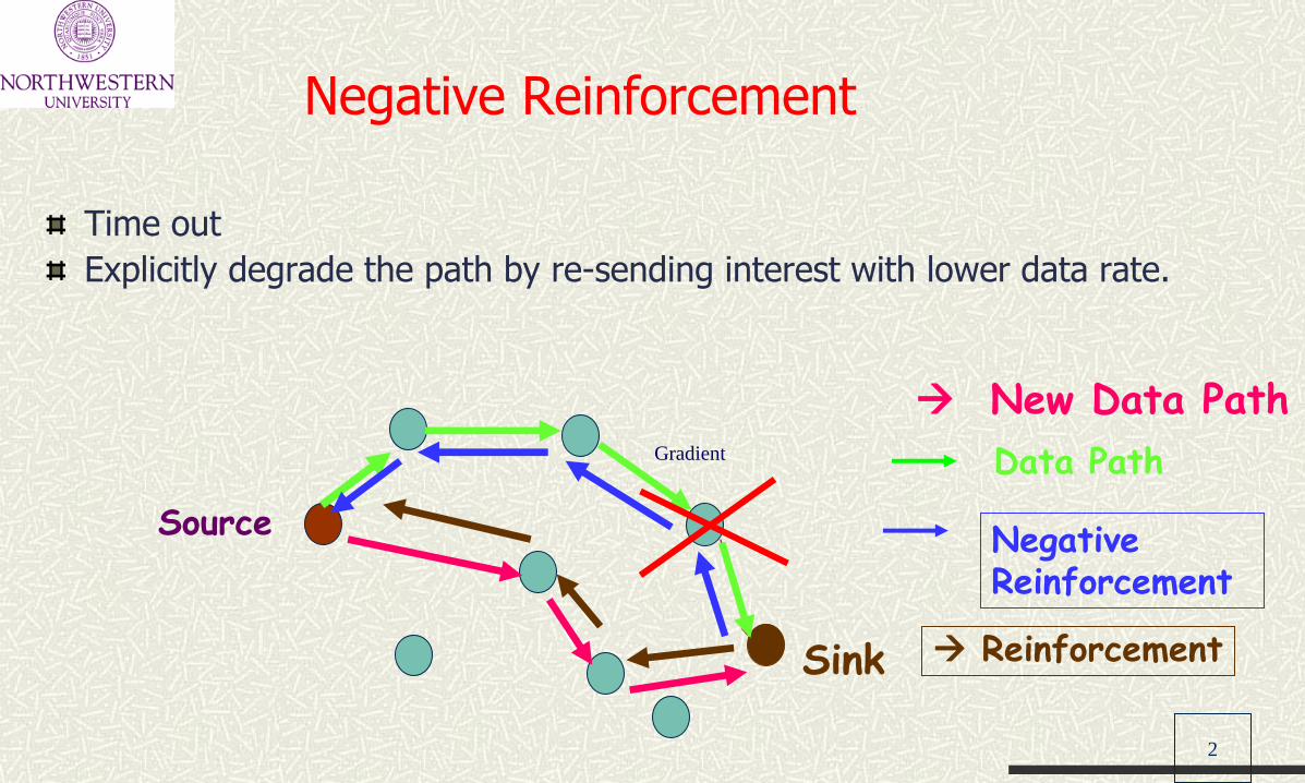
Negative Reinforcement
Time out
Explicitly degrade the path by re-sending interest with lower data rate.
Source
Gradient Data Path
Sink
Negative Reinforcement
Reinforcement
New Data Path
3
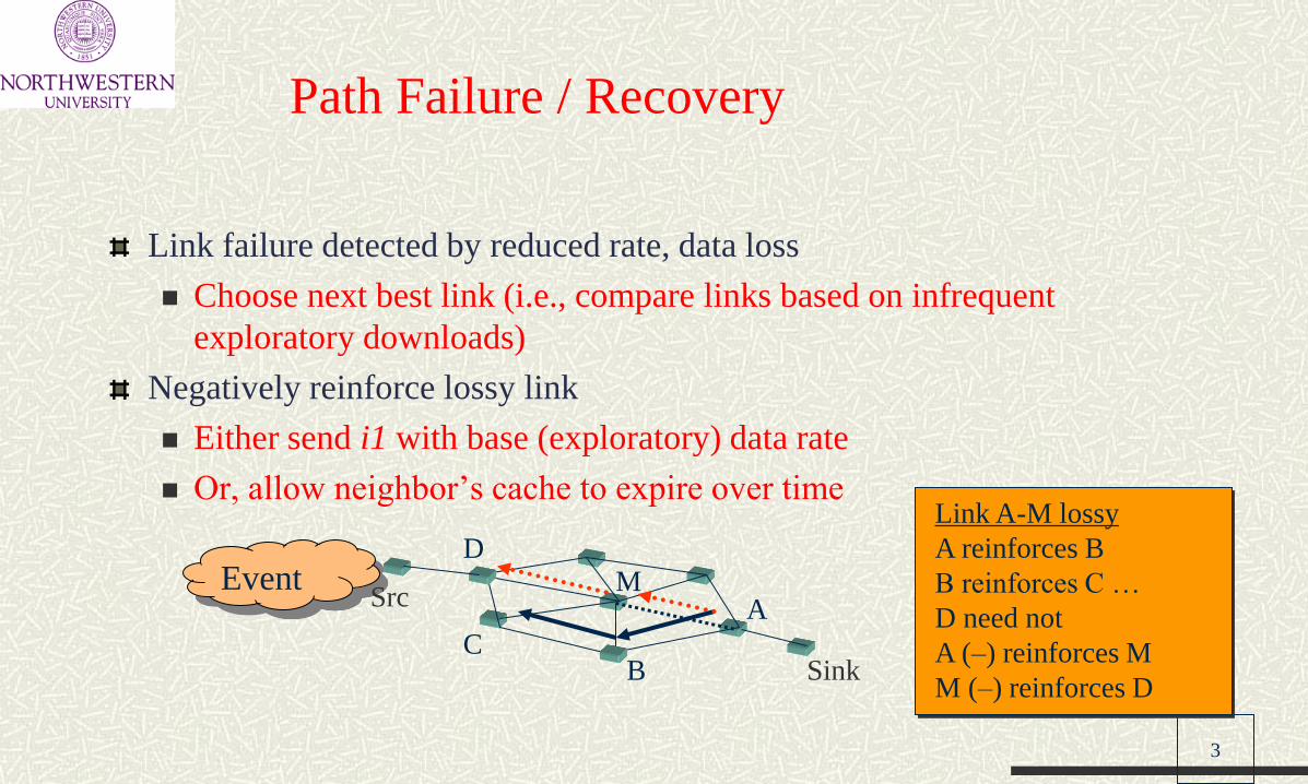
Path Failure / Recovery
Link failure detected by reduced rate, data loss
Choose next best link (i.e., compare links based on infrequent
exploratory downloads)
Negatively reinforce lossy link
Either send i1 with base (exploratory) data rate
Or, allow neighbor’s cache to expire over time
Event
Sink
Src A
C B
M D
Link A-M lossy
A reinforces B
B reinforces C …
D need not
A (–) reinforces M
M (–) reinforces D
4
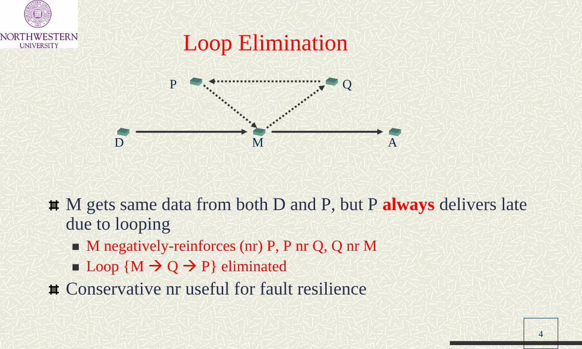
M gets same data from both D and P, but P always delivers late due to looping
M negatively-reinforces (nr) P, P nr Q, Q nr M
Loop {M Q P} eliminated
Conservative nr useful for fault resilience
Loop Elimination
A
Q P
D M

5
Local Behavior Choices
1. For propagating interests
In our example, flooding
More sophisticated behaviors possible: e.g. based on cached information, GPS
2. For setting up gradients
Highest gradient towards neighbor from whom we first heard interest
Others possible: towards neighbor with highest energy
3. For data transmission
Different local rules can result in single path
delivery, multi-path delivery, single source
to multiple sinks …
4. For (negative) reinforcement
reinforce one path, or part thereof, based on
observed losses, delay variances etc.
other variants: inhibit certain paths because
resource levels are low

6
Simulation
Simulator: ns-2
Network Size: 50-250 Nodes
Total area for 50 nodes 160m x 160m
Transmission Range: 40m
Constant Density: 1.95x10⁻³ nodes/m2 (9.8 nodes in radius)
MAC: Modified Contention-based MAC
Energy Model: Mimic a realistic sensor radio
660 mW in transmission, 395 mW in reception, and 35 mw in idle
7
Performance Metrics
Average Dissipated Energy
Ratio of total dissipated energy per node in the network to the number of distinct events seen by sinks.
Average Delay
Average one-way latency observed between transmitting an event and receiving it at each sink.
Event Delivery Ratio
Ratio of the number of distinct events received to number originally sent.

8
Average Dissipated Energy (Sensor Radio Energy Model)
0
0.002
0.004
0.006
0.008
0.01
0.012
0.014
0.016
0.018
0 50 100 150 200 250 300
Ave
rage
Dissipa
ted E
nerg
y
(Jou
les/
Nod
e/R
ece
ived E
vent
)
Network Size
Diffusion
Flooding
Diffusion outperforms flooding. WHY ?
9
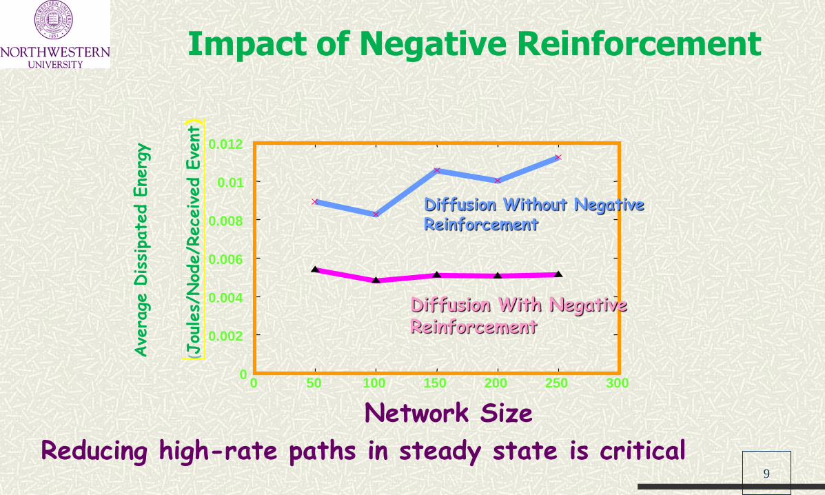
Impact of Negative Reinforcement
0
0.002
0.004
0.006
0.008
0.01
0.012
0 50 100 150 200 250 300
Ave
rage
Dissipa
ted E
nerg
y
(Jou
les/
Nod
e/R
ece
ived E
vent
)
Network Size
Diffusion With Negative Reinforcement
Diffusion Without Negative Reinforcement
Reducing high-rate paths in steady state is critical

10
Directed Diffusion – Extensions
Two-Phase Pull suffers from interest flooding problems
Push Diffusion – Data Advertisement by the Sources
Sink sends reinforcement packet.

11
Directed Diffusion vs SPIN
• In DD Sink queries sensors if a specific data is
available by flooding some interests.
In SPIN Sensors advertise the availability of data
allowing sinks to query that data.

12
Directed Diffusion Advantages
* DD is data centric no need for a node addressing mechanism.
* Each node is assumed to do aggregation, caching and sensing.
* DD is energy efficient since it is on demand
and no need to maintain global network topology.
13
Directed Diffusion Disadvantages
• Not generally applicable since it is based on a query driven
data delivery model.
• For DYNAMIC applications needing continuous data delivery
(e.g., environmental monitoring) DD is not a good choice.
• Naming schemes are application dependent and each time
must be defined a-priori.
• Matching process for data and queries cause some overhead
at sensors.

14
Rumor Routing
Motivation
Sometimes a non-optimal route is satisfactory
Advantages Tunable best effort delivery
Tunable for a range of query/event ratios
Disadvantages Optimal parameters depend heavily on topology (but can be adaptively tuned)
Does not guarantee delivery
Designed for query/event ratios between query and event flooding

15
Rumor Routing

16
Basis for Algorithm
Observation: Two lines in a
bounded rectangle have a 69%
chance of intersecting
Create a set of straight line
gradients from event, then send
query along a random straight line
from source until it meets an event
line.
Event
Q-Source
17
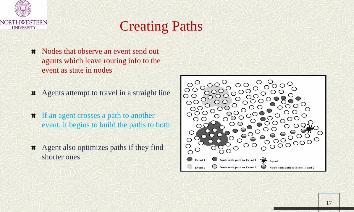
Creating Paths
Nodes that observe an event send out
agents which leave routing info to the
event as state in nodes
Agents attempt to travel in a straight line
If an agent crosses a path to another
event, it begins to build the paths to both
Agent also optimizes paths if they find
shorter ones

18
Algorithm Basics
All nodes maintain a neighbor list
Nodes also maintain an event table
When it observes an event, the event is added with distance 0
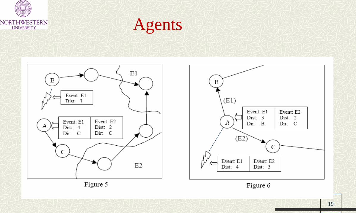
Agents
Packets that carry local event info across the network
Aggregate events as they go
Agents do a random walk: among the one-hop neighbors, find the one that was not visited recently.
19
Agents

20
Agent Path
Agent tries to travel in a “somewhat” straight path
Maintains a list of recently seen nodes (RSN)
When it arrives at a node it adds the node’s neighbors to the list RSN
It next tries to find a node not in RSN
-this avoids loops
Important to find a path regardless of “quality”

21
Query propagation--following paths
A query originates from a source, and is forwarded along until it reaches
the event or it’s TTL expires
Forwarding Rules:
If a node has a route to the event, it forwards the query to the neighbor
along the route
If a node has seen the query before, it forwards it to a neighbor using a
straightening algorithm (query also keeps track of RSN)

22
Hierarchical Protocols
Hierarchical-architecture protocols are proposed to address
the scalability and energy consumption challenges of sensor
networks.
Sensor nodes form clusters where the cluster-heads
aggregate and fuse data to conserve energy.
The cluster-heads may form another layer of clusters
among themselves before reaching the sink.

23
Hierarchical Protocols
Low-Energy Adaptive Clustering Hierarchy (LEACH) (Heinzelman’02)
Power-efficient GAthering in Sensor Information Systems (PEGASIS)
Threshold sensitive Energy Efficient sensor Network protocol (TEEN)
Adaptive Threshold sensitive Energy Efficient sensor Network
protocol (APTEEN)

24
LEACH Protocol Architecture
Low-Energy Adaptive Clustering Hierarchy
Adaptive, self-configuring cluster formation
Localized control for data transfers
Low-energy medium access control
Application-specific data aggregation
Base station
Cluster-head
25
.
Idea: * Randomly select sensor nodes as cluster heads, so the high energy
dissipation in communicating with the base station is spread to all
sensor nodes in the network.
* Forming clusters is based on the received signal strength.
* Cluster heads can then be used kind of routers (relays) to the
sink.
-
Low Energy Adaptive Clustering Hierarchy W. R. Heinzelmn, A. Chandrakasan, and H. Balakrishnan,
“Energy-Efficient Communication Protocol for Wireless Microsensor
Networks,'' IEEE Tr. on Wireless Com., pp.660-670, Oct. 2002

26
Dynamic Clusters
Cluster-head rotation to evenly distribute energy load
Adaptive clusters
Clusters formed during set-up
Scheduled data transfers during steady-state
Time •••
START START START
Set-up Frame Round Steady-state
Cluster-heads = •

27
Distributed Cluster Formation
Ci(t) = 1 if node i a CH in
last r mod (N/k) rounds
Each node CH once in N/k rounds
0
)/mod(* )(Pi kNrkN
k
t0 )(Ci t
1 )(Ci t
Assume nodes begin with equal energy
Design for k clusters per round
Want to evenly distribute energy load
Can determine Pi(t) with unequal node energy
ktN
i
1)(P CH] E[#1
i
k = system param.
(Analytical optimum)

28
LEACH
• After the cluster heads are selected, the cluster heads
advertise to all sensor nodes in the network that they are
the new cluster heads.
• Each node accesses the network through the cluster head that
requires minimum energy to reach.

29
LEACH
Once the nodes receive the advertisement, they determine the cluster
that they want to belong based on the received signal strength of the
advertisement from the cluster heads to the sensor nodes.
The nodes inform the appropriate cluster heads that they will be a
member of the cluster.
Afterwards the cluster heads assign the time slots during which the sensor
nodes can send data to them.

30
Set-up Steady-state
LEACH Steady-State
Cluster-head coordinates transmissions
Time Division Multiple Access (TDMA) schedule
Node i transmits once per frame
Cluster-head broadcasts TDMA schedule
Low-energy approach
No collisions
Maximum sleep time
Power control
Clusters formed
Time
Slot for
node i
Slot for
node i •••
Frame

31
Distributed Cluster Formation
Using Pi(t)
Choose CH with “loudest”
announcement
Cluster-head
Nodes Non-CH
Nodes
Node i
cluster-head ?Yes No
Wait for
cluster-head
announcements
Send Join-Request
message to chosen
cluster-head
Announce
cluster-head status
Wait for
Join-Request
messages
Steady-state
operation for
t=Tround
seconds
Autonomous decisions lead to global behavior
• No global control
• Flexible, fault-tolerant

32
LEACH
STEADY STATE PHASE:
Sensors begin to sense and transmit data to the cluster
heads which aggregate data from the nodes in their
clusters.
After a certain period of time spent on the steady state,
the network goes into start-up phase again and enters
another round of selecting cluster heads.

33
Base Station Cluster Formation
Get optimal clusters for comparison
LEACH-C
Requires communication with base station
Nodes send base station current position
Base station runs optimization algorithm to determine best
clusters
Need GPS or other location-tracking method

34
Simulation Parameters
500 bytes Data size
5 nJ/bit/signal Aggregation cost
100 pJ/bit/m2 Transmit amplifier
50 nJ/bit Radio electronics
100 kbps Bit rate
50 ms Processing delay
Base Station
75 meters
100 m
ete
rs
100 meters
100 nodes
35
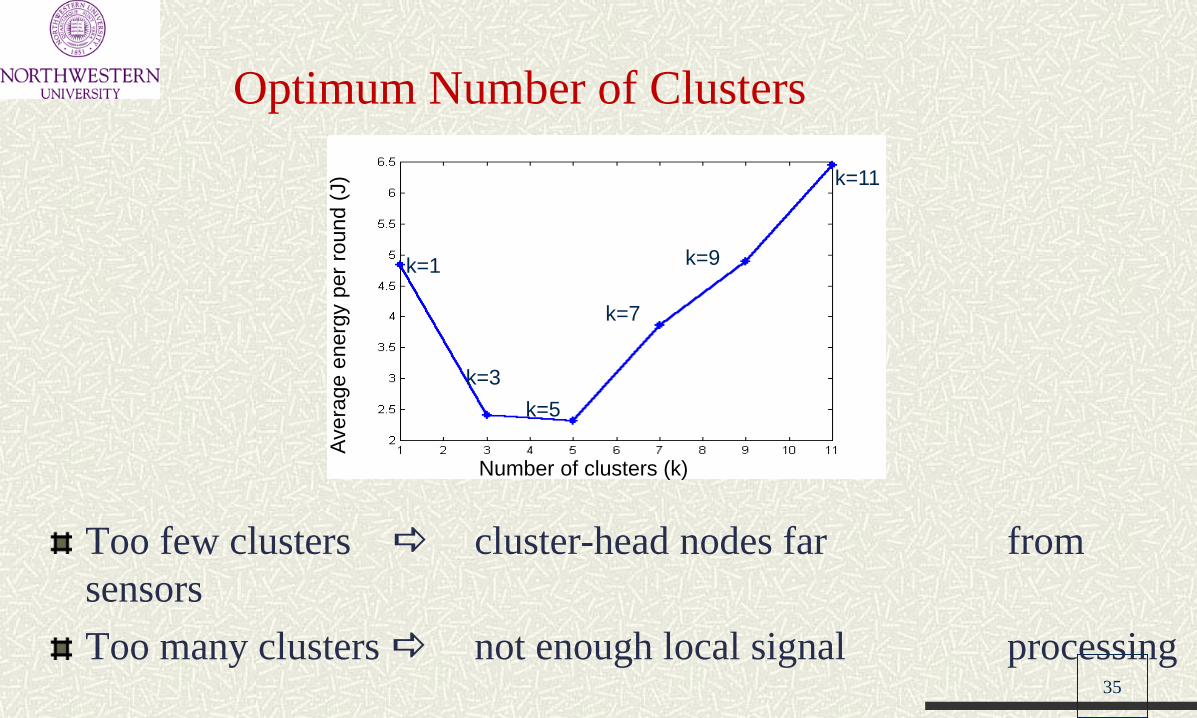
Optimum Number of Clusters
Avera
ge e
nerg
y p
er
round (
J)
Number of clusters (k)
k=7
k=9
k=5
k=3
k=1
k=11
Too few clusters cluster-head nodes far from
sensors
Too many clusters not enough local signal processing
36
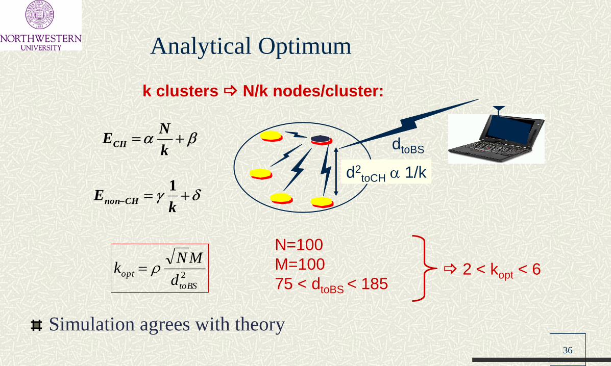
Analytical Optimum
k
E CHnon
1
k clusters N/k nodes/cluster:
2
toBS
optd
MNk
N=100
M=100
75 < dtoBS < 185 2 < kopt < 6
Simulation agrees with theory
k
NECH dtoBS
d2toCH 1/k
37
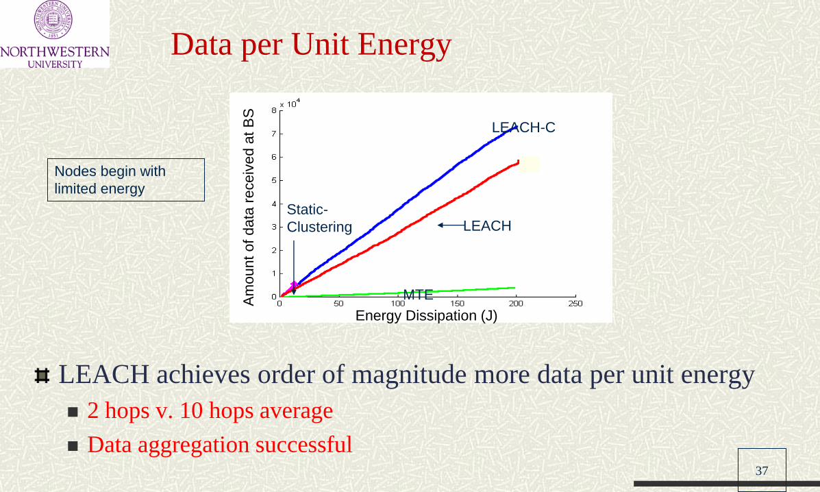
Data per Unit Energy
Am
ount
of
data
receiv
ed a
t B
S
Energy Dissipation (J)
Static-
Clustering
LEACH-C
LEACH
MTE
LEACH achieves order of magnitude more data per unit energy
2 hops v. 10 hops average
Data aggregation successful
Nodes begin with
limited energy
38
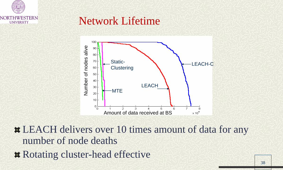
Network Lifetime
Num
ber
of
nodes a
live
Amount of data received at BS
Static-
Clustering LEACH-C
LEACH MTE
LEACH delivers over 10 times amount of data for any number of node deaths
Rotating cluster-head effective

39
LEACH - CONCLUSIONS
It is not applicable to networks deployed in
large regions.
Furthermore, the idea of dynamic clustering
brings extra overhead, e.g., head changes,
advertisements etc. which may diminish the
gain in energy consumption.